Discrimination of two channels by adaptive methods and its application to quantum system

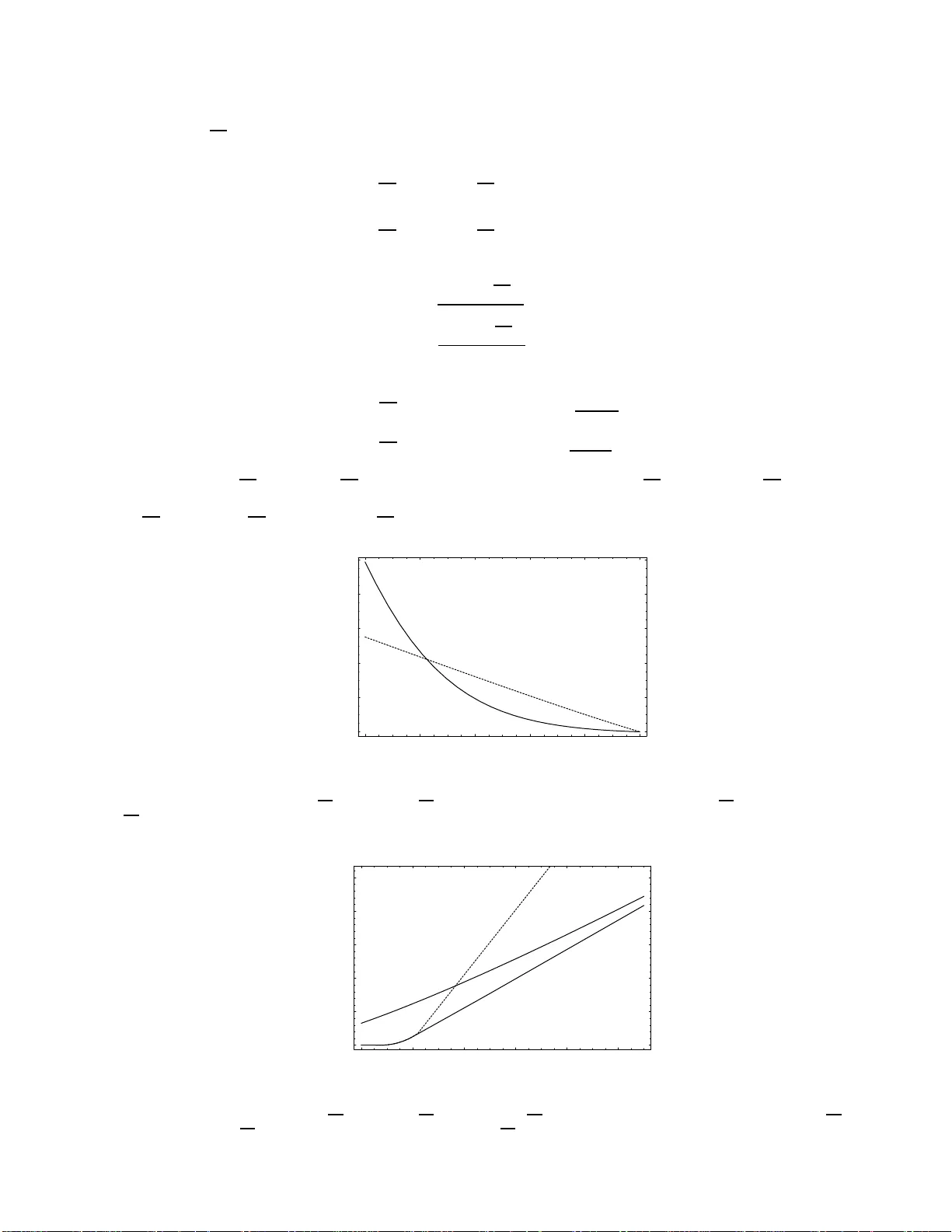
1 Discriminati on of t wo channels by adapti v e methods and its applic ation to quantum system Masahito Hayash i Abstract The optimal exponen tial error rate for ada ptiv e discrimination of two chann els i s discussed. In this problem, adapti ve choice of input signal i s allo wed. This problem is discussed in v arious settings. I t is pro v ed that adapti v e choice does not impro ve t he expo nential error rate in these settings. These results are applied to quantum state discrimination. Index T erms Simple hypothesis testing, Channel, Discrimination, Quantum state, One-way LOCC, Acti ve learning , Experimental design, Stein’ s lemma, Chernoff bound, Hoef fding bound, Han-Ko bayashi bound I . I N T R O D U C T I O N D ISCRIMIN A TING two distributions is treated as a fun damental problem in the field of statistical inferen ce. This problem can b e regarded as simple hypothesis testing because both hypotheses con sist of a single distribution. Many researchers, Stein, Chernoff[3], Hoef fding[16], and Han-K obayashi[1 0 ] hav e studied the asymptotic behavior when the number n of identical and independen t observations is sufficiently large. They formulated a simple h ypothesis testing/d iscrimination o f two distrib utions as an optimization problem an d d erived the respecti ve optimu m value, e. g., the optimal exponen tial erro r rate. W e call th ese op timum values the Stein bou nd, the Cher noff b ound , the Hoeffding bound, and the Han-K obayashi bound, respectively . Han [8], [9] later extended these results to the discriminatio n of two general sequences of distributions, including the Markovian case. Nagaoka-Hayashi [21] simplified Han’ s discussion and gener alized Han’ s extension of the Han-K obayashi bound . In th e pre sent pap er , w e c onsider an other extension of the ab ove results. That is, we extend the above results to the discrimination of two (classical) channels, in which two p robabilistic transition matric es are g iv en. Such a prob lem has appea red in Blahut[2]. In this problem , th e numb er o f applications of this channel is fixed to a gi ven co nstant n , and we can choose approp riate inputs for this purpose. I n th is case, we assume that the gi ven chann el is memoryless. If we use the same in put to all applications of the gi ven chan nel, the n output d ata obeys an ide ntical and independ ent distribution. T his prope rty ho lds ev en if we choose the input ran domly based on the same distribution on in put signals. This strategy is called the non-ad aptive method. In p articular, when the same input is applied to all ch annels, it is called the de terministic non-ad aptive method. If the inpu t is determined stochastically , it is called the sto chastic non-ad aptive meth od, which was treated by Blah ut[2]. In the non-ad aptive method, our task is cho osing the optimal input for d istinguishing two channels most efficiently . In the presen t paper, we assume that we can choose the k -th input signal b ased on the prece ding k − 1 output data. This strategy is called the adaptive method , which is the m ain f ocus of the p resent paper . In th e param eter estimation, such an a daptive metho d impr oves estimation perf ormanc e. That is, in the one-param eter estimation , the asymptotic estimation err or is boun ded by the in verse of th e optimum Fisher information. Howe ver , if we d o not apply the adaptive method, it is generally impossible to realize the optimum Fisher informatio n in all p oints at the same time. It is kn own that the adap tiv e metho d rea lizes th e optimum Fisher information in all points[1 3], [7]. Therefore, one may expect that the adap tiv e method improves the perform ance of discriminating two chan nels. As o ur main resu lt, we succeeded in pr oving that the ad aptive metho d canno t improve the non-ad aptive method in the sense of all of the above men tioned boun ds, i.e., the Stein bound, the Ch ernoff bound, the Hoef fding bound, and th e Han- K obayashi bou nd. Th at is, there is no difference between the no n-adap tiv e method and the a daptive method in these asy mptotic formu lations. Ind eed, as is p roven herein, the deterministic non-adaptive m ethod gi ves the optimu m p erform ance with respect to th e Stein bo und, the Chernoff boun d, and the Ho effding bound . Howe ver , in order to attain the Han-K obayashi boun d, in general, we need th e stochastic non -adaptive m ethod. On the o ther han d, the researc h field in q uantum inform ation has treated the discrimination of two quantum states. H iai- Petz[15] and Ogawa-Nagaoka[18 ] proved the quantum version of Stein’ s le mma. Audenaert et al. [ 1] and Nussbaum-Szkoła [23], [24] obtain ed the quantu m version o f the Chern off boun d. Ogawa-Hayashi [ 17] de riv ed a lower bound o f the quantum version of the Hoeffding b ound . Later , Hayashi [12] a nd Nagaoka [20] o btained its tight bo und based on the results by Aud enaert et al. [1] an d Nussbaum- Szkoła [23], [24]. Hayashi [11] ( in p.90 ) obtain ed the q uantum version of th e Han- K obayashi bou nd based on Na gaoka[ 19 ]’ s discussion. These discussions M. Hayashi is with Graduate School of Information Sciences, T ohoku Univ ersity , Aoba-ku , Senda i, 980-8579, Japan (e-mail: hayashi@math.is.tohoku .ac.jp) 2 assume that any measurement o n the n -tensor product system is allowed fo r testing the g iv en state. Hence, the next go al is the deriv ation of these bou nds under some locality restrictio ns on an n -par tite system for possible measur ements. One easy setting is restricting the present m easurement to be identical to that in the respective system. In this case, our task is the choice of the o ptimal measurement on the sing le system. By considering the mea surement an d the quantum state as th e input and the ch annel, respectively , we c an treat this problem by the no n-adap tiv e method of the classical channel. Another setting is restricting o ur measure ment to one-way local oper ations and classical communicatio ns (o ne-way LOCC). In the above- mentioned c orrespon dence, the o ne-way LOCC setting can be regarded as the ad aptive metho d of the classical chann el. He nce, applying the above argu ment to d iscrimination of two qu antum states, we can conclude that one-way co mmunica tion do es no t improve discr imination of two quan tum states in the respective asymptotic formulations. Furthermo re, the same p roblem appears in adap tiv e experimental d esign and active learnin g. In learning theory , we id entify the given system by using th e obtained sequ ence of inp ut and o utput pairs. In particular , in acti ve learning, we can ch oose the inputs using the precedin g d ata. Hence, the present result indicates that acti ve learning does not improve th e perfor mance of learning when the candidates of the unknown system are gi ven by o nly two classical channels. I n experimental d esign, we choose su itable design of o ur experim ent for inferrin g th e unk nown para meter . Ad aptive improvement for the design is allowed in adap tiv e experimen tal design. When the candida tes o f the un known par ameter are only two values, the obtained result can be applied. Th at is, adaptive impr ovement for design d oes not work. The r emainder of th e pre sent paper is organized as follows. Section II r evie ws the Stein bo und, the Chernoff bo und, the Hoeffding bound, and the Han-K obayashi bound in discrimination of two p robab ility distrib utions. In Sec tion III, we present our fo rmulation an d notatio ns of the adap ti ve method in the discrimin ation of two (classical) chann els, and d iscuss the adap tiv e- method versions of the Stein bound, the Cher noff boun d, the Ho effding bo und, and the Han-K obayashi b ound , r espectively . In Section I V, we co nsider a simple examp le, in which the stochastic non-adap ti ve metho d is requir ed for attaining the Ha n- K obayashi bound. In Sec tion V, we apply the present result to discrimination o f two quantum states by o ne-way LOCC. In Sections VI, VI I, and VI II, we prove the adaptive-method version s of Stein bound, th e Chernoff b ound , the Hoeffding boun d, and the Han-Kobayashi bound, respectiv ely . I I . D I S C R I M I N A T I O N / S I M P L E H Y P OT H E S I S T E S T I N G B E T W E E N T W O P RO B A B I L I T Y D I S T R I B U T I O N S In prepar ation for th e main to pic, we review the simple hyp othesis testing p roblem fo r the n ull hy pothesis H 0 : P n versus the alternative hyp othesis H 1 : P n , wh ere P n and P n are the n -th identical and indepen dent distributions of P an d P , re spectiv ely on the pro bability spa ce Y . Th e p roblem is to decide wh ich h ypoth esis is true based on n o utputs y 1 , . . . , y n . In the following, random ized tests are allowed as our decision. Hence, our d ecision method is described by a [0 , 1] -valued functio n f on Y n . When we observe n outputs y 1 , . . . , y n , we ac cept the alternativ e hypo thesis P with the probability f ( y 1 , . . . , y n ) . W e have two types of erro rs. In the first ty pe, the null hypothesis P is rejected despite being cor rect. In th e seco nd type , the alternative P is rejected d espite bein g cor rect. Hence, the first ty pe of error prob ability is given by E P n f , and the second ty pe of error probab ility is by E P n (1 − f ) . Note that E P describes the expecta tion u nder the distribution P . In the fo llowing, we assume that Φ( s | P k P ) := Z Y ( ∂ P ∂ P ( y )) s P ( d y ) < ∞ φ ( s | P k P ) := log Φ( s | P k P ) and φ ( s | P k P ) is C 2 -continu ous. In th e p resent p aper, we choo se the base o f the logarithm to be e . In the discrim ination o f two distrib utions, we treat two types of proba bilities equally . Then, we simply minimize the equ al sum E P n f + E P n (1 − f ) . Its optimal rate of exponential d ecrease is charac terized by the Chernoff bound[3]: C ( P , P ) := lim n →∞ − 1 n log(min f n E P n f n + E P n (1 − f n )) = − min 0 ≤ s ≤ 1 φ ( s | P k P ) . In order to tr eat these two erro r pro babilities asymm etrically , we often restrict the first type of erro r pro bability E P n f to b elow a particu lar threshold ǫ , and min imize the second type of e rror proba bility E P n (1 − f ) : β ∗ n ( ǫ ) := min f  E P n (1 − f )   E P n f ≤ ǫ  . Then, the Stein’ s lemma holds. For 0 < ∀ ǫ < 1 , the eq uation lim n →∞ 1 n log β ∗ n ( ǫ ) = − D ( P k P ) (1) holds, where the re lativ e entropy D ( P k P ) is defined by D ( P k P ) = Z Y − log ∂ P ∂ P ( y ) P ( dy ) . 3 Indeed , this lemma has the following variant for m. Define B ( P k P ) := sup { f n }  lim n →∞ − log E P n (1 − f n ) n     lim n →∞ E P n f n = 0  B ∗ ( P k P ) := inf { f n }  lim n →∞ − log E P n (1 − f n ) n     lim n →∞ E P n f n < 1  . Then, these two qua ntities satisfy the following relations: B ( P k P ) = B ∗ ( P k P ) = D ( P k P ) . As a furth er analysis, we focus on the decreasin g e xponen t o f the error prob ability of the first type under an expon ential constraint for the err or proba bility of the seco nd type . When the decrea sing expon ent of for the error pr obability of the seco nd type is greater than the relative entro py D ( P k P ) , the e rror probability of the second type con verges to 1 . In this case, we focus on the decr easing exponen t of th e probab ility of correctly accepting the nu ll hypothesis P . For th is purp ose, we define B e ( r | P k P ) := sup { f n }  lim n →∞ − log E P n f n n     lim n →∞ − log E P n (1 − f n ) n ≥ r  B ∗ e ( r | P k P ) := inf { f n }  lim n →∞ − log E P n (1 − f n ) n     lim n →∞ − log E P n (1 − f n ) n ≥ r  . Then, the two qu antities are calculated as B e ( r | P k P ) = min Q : D ( Q k P ) ≤ r D ( Q k P ) = sup 0 ≤ s ≤ 1 − sr − φ ( s | P k P ) 1 − s (2) B ∗ e ( r | P k P ) = min Q : D ( Q k P ) ≤ r D ( Q k P ) + r − D ( Q k P ) = sup s ≤ 0 − sr − φ ( s | P k P ) 1 − s . (3) The first expressions of (2) a nd (3) are illustrated b y Figs. 1 a nd 2. P P Q ( ) D Q P r = ( ) D Q P Fig. 1. Figu re of B e ( r | P k P ) P P Q ( ) D Q P r = Fig. 2. Figu re of B ∗ e ( r | P k P ) when r 0 ≥ r ≥ D ( P k P ) 4 Now , we define the new function B ( r ) : B e ( r ) :=  B e ( r | P k P ) r ≤ D ( P k P ) − B ∗ e ( r | P k P ) r > D ( P k P ) . Then, its gr aph is shown in Fig. 3. ( ) D P P ( ) e B r ( ) D P P r Graph of ( ) e B r ( ) , C P P 0 r Fig. 3. Graph of B e ( r ) In order to g iv e other characterization s o f (2), we in troduce a one-p arameter family P s,P, P ( dy ) := 1 Φ( s | P k P ) ( ∂ P ∂ P ( y )) s P ( d y ) , which is abbr eviated as P s . Then, since φ ( s ) is C 1 continuo us, D ( P s k P 1 ) = ( s − 1) φ ′ ( s ) − φ ( s ) s ∈ ( −∞ , 1 ] (4) D ( P 0 k P s ) = φ ( s ) − sφ ′ (0) s ∈ [0 , ∞ ) . (5) Since d ( s − 1) φ ′ ( s ) − φ ( s ) ds = − φ ′′ ( s ) < 0 , D ( P s k P 1 ) is mo noton ically d ecreasing with respect to s . As is men tioned in Theore m 4 of Blahut [2], whe n r ≤ D ( P k P ) , there exists s r ∈ [0 , 1] such that min Q : D ( Q k P ) ≤ r D ( Q k P ) = D ( P s r k P 0 ) . Then, (4) and (5) imply that r = D ( P s r k P 1 ) = ( s r − 1) φ ( s r ) − φ ( s r ) . Thus, we ob tain another expression. min Q : D ( Q k P ) ≤ r D ( Q k P ) = min s ∈ [0 , 1]: D ( P s k P ) ≤ r D ( P s k P ) . (6) On the othe r hand, d ds − sr − φ ( s | P k P ) 1 − s = − r + ( s − 1) φ ′ ( s ) − φ ( s ) (1 − s ) 2 = D ( P s k P 1 ) (1 − s ) 2 . (7) Since D ( P s k P 1 ) is mono tonically decreasing with respect to s , d ds − sr − φ ( s | P k P ) 1 − s = 0 if an d only if s = s r . The equ ation min Q : D ( Q k P ) ≤ r D ( Q k P ) = sup 0 ≤ s ≤ 1 − sr − φ ( s | P k P ) 1 − s (8) can be ch ecked. 5 In the following, we present som e explanation s co ncernin g (3). As is m entioned by Han-K obayashi[ 10 ] and Og awa- Nagaoka[ 18 ], when r 0 := D ( P −∞ k P 1 ) ≥ r ≥ D ( P k P ) , the relation B ∗ e ( r | P k P ) = D ( P s r k P 0 ) holds, where s r ∈ ( −∞ , 0 ] is define d as r = D ( P s r k P 1 ) = ( s r − 1) φ ( s r ) − φ ( s r ) . Thus, similar to (6) and (8), the relation min Q : D ( Q k P ) ≤ r D ( Q k P ) + r − D ( Q k P ) = D ( P s r k P ) = sup s ≤ 0 − sr − φ ( s | P k P ) 1 − s (9) holds, where s r ≤ 0 is defined by D ( P s r k P ) = r [ 18]. As mention ed by Nakagawa-Kanaya[22 ], when r ≥ r 0 , the r elation min Q : D ( Q k P ) ≤ r D ( Q k P ) + r − D ( Q k P ) = D ( P −∞ k P ) + r − D ( P −∞ k P ) = min Q : D ( Q k P ) ≤ r 0 ( D ( Q k P ) + r 0 − D ( Q k P )) + r − r 0 holds. This bound is attained by the following ran domized test. The hypoth esis P is acce pted with the probability only when the loga rithmic likelihood ratio takes the maximum value r 0 . Since D ( P s k P 1 ) < r , (7) implies that sup s ≤ 0 − sr − φ ( s | P k P ) 1 − s = lim s ≤−∞ − sr − φ ( s | P k P ) 1 − s = lim s ≤−∞ − sr 0 − φ ( s | P k P ) 1 − s + r − r 0 = min Q : D ( Q k P ) ≤ r 0 ( D ( Q k P ) + r 0 − D ( Q k P )) + r − r 0 . (10) Remark 1: The classical Hoeffding bound in information theory is due to Blahut[2] and Csisz ´ ar-Longo[4]. The correspondin g ideas in statistics were first put f orward by Hoeffding[16], from whom the b ound recei ved its name. So me authors p refer to refer this bo und as the Hoeffding-Blahu t-Csisz ´ ar - Long o bound. On the other hand, Han-K obayashi[1 0 ] ga ve th e first equation of (3), and proved that this equa tion a mong non- rando mized tests when r 0 ≥ r ≥ D ( P k P ) . They po inted out that the minim um min Q : D ( Q k P ) ≤ r D ( Q k P ) + r − D ( Q k P ) can be attained by Q satisfyin g D ( Q k P ) = r . Ogawa-Nagaoka[18 ]sho wed the second equ ation of (3) for this case. Nakagawa-Kanaya[2 2 ] proved the first equation when r > r 0 . I ndeed, as pointed by Nakagawa-Kanaya[22 ], when r > r 0 , any non-rand omized test cannot attain the minimu m min Q : D ( Q k P ) ≤ r D ( Q k P ) + r − D ( Q k P ) . In this case, the m inimum min Q : D ( Q k P ) ≤ r D ( Q k P ) + r − D ( Q k P ) cannot be attained by Q satisfying D ( Q k P ) = r . I I I . M A I N R E S U LT : A DA P T I V E M E T H O D Let us focus on two spaces, the set of inp ut signals X and the set of outputs Y . I n this case, the channel f rom X an d Y is described by the map f rom th e set X to the set of pro bability distributions on Y . That is, gi ven a chann el W W x represents the outpu t d istribution when the input is x ∈ X . When X and Y have finite elements, the channel is giv en by transition matrix. The main topic is th e discriminatio n of two classical chann els W and W . In p articular, we treat its asy mptotic an alysis when we can use the unk nown channel only n times. That is, we discrim inate two hypo theses, the null hypo thesis H 0 : W n versus the alternative hypoth esis H 1 : W n , where W n and W n are the n u ses of th e ch annel W and W Then, o ur problem is to de cide which hypo thesis is tru e b ased on n inputs x 1 , . . . , x n and n outp uts y 1 , . . . , y n . I n th is setting, it is allo wed to choose th e k -th input based on the previous k − 1 outp ut adaptively . W e choose th e k -th inp ut x k subject to the d istribution P k ( x 1 ,y 1 ) ,..., ( x k − 1 ,y k − 1 ) ( x k ) o n X . That is, the k -th input x k depend s on k conditional distributions ~ P k = ( P 1 , P 2 , . . . , P k ) . Hence, our decision method is de scribed by n co nditiona l distributions ~ P n = ( P 1 , P 2 , . . . , P n ) and a [0 , 1] -valued fun ction f n on ( X × Y ) n . In th is case, wh en we ch oose n in puts x 1 , . . . , x n and ob serve n ou tputs y 1 , . . . , y n , we accept the a lternative hypoth esis W with the pro bability f n ( x 1 , y 1 , . . . , x n , y n ) . That is, our scheme is illustrated by Fig. 4. In orde r to treat this problem mathematically , we introdu ce th e following n otation. For a channel W fro m X to Y an d a distribution P on X , we define two no tations, the distribution W P on X × Y and th e distribution W · P o n Y as W P ( x, y ) := W x ( y ) P ( x ) W · P ( x, y ) := Z X W x ( y ) P ( dx ) . Using the distribution W P , we d efine two quantities: D ( W k W | P ) := D ( W P k W P ) φ ( s | W k W | P ) := φ ( s | W P k W P ) . 6 Channel discr imination with adaptive improv ement 1 x 1 y 2 y n y 2 x n x Adaptive improvement is allowed or W W or W W or W W Fig. 4. The adapti ve method Based on k cond itional distributions ~ P k = ( P 1 , P 2 , . . . , P k ) , we defin e the following distrib utions: Q W , ~ P n := W P n W P n − 1 · · · W P 1 P W , ~ P n := P n · Q W , ~ P n − 1 Q s,W | W , ~ P n := P s,Q W, ~ P n ,Q W , ~ P n P s,W | W , ~ P n := P n · Q s,W | W , ~ P n − 1 . Then, the first type of erro r probab ility is g iv en b y E Q W, ~ P n f n , and th e second ty pe of erro r probab ility is by E Q W , ~ P n (1 − f n ) . In order to tre at this pro blem, we introduc e the follo wing quantities: C ( W, W ) := lim n →∞ − 1 n log( min ~ P n ,f n E Q W, ~ P n f n + E Q W , ~ P n (1 − f n )) β ∗ n ( ǫ ) := min ~ P n ,f n  E Q W , ~ P n (1 − f n )   E Q W, ~ P n f n ≤ ǫ  , and B ( W k W ) := sup { ( ~ P n ,f n ) } ( lim n →∞ − log E Q W , ~ P n (1 − f n ) n      lim n →∞ E Q W, ~ P n f n = 0 ) B ∗ ( W k W ) := inf { ( ~ P n ,f n ) } ( lim n →∞ − log E Q W , ~ P n (1 − f n ) n      lim n →∞ E Q W, ~ P n f n < 1 ) B e ( r | W k W ) := sup { ( ~ P n ,f n ) } ( lim n →∞ − log E Q W, ~ P n f n n     lim n →∞ − log E Q W , ~ P n (1 − f n ) n ≥ r ) B ∗ e ( r | W k W ) := inf { ( ~ P n ,f n ) } ( lim n →∞ − log E Q W, ~ P n (1 − f n ) n      lim n →∞ − log E Q W , ~ P n (1 − f n ) n ≥ r ) . W e obtain the following channel version of Stein’ s lemm a. Theor em 1: Assume that φ ( s | W x k W x ) is C 1 continuo us, an d lim ǫ → +0 φ ( − ǫ | W k W ) ǫ = sup x ∈X D ( W x k W x ) , (11) where φ ( s | W k W ) := sup x ∈X φ ( s | W x | W x ) = sup P ∈P ( X ) φ ( s | W k W | P ) , and P ( X ) is the set of distributions on X . Then, B ( W k W ) = B ∗ ( W k W ) = D := sup x ∈X D ( W x k W x ) . (12) The following is another expression of Stein’ s lemma. 7 Cor o llary 1: Under the same assumptio n, lim n →∞ − 1 n log β ∗ n ( ǫ ) = sup x ∈X D ( W x k W x ) . Condition (11) can b e replaced by an other condition . Lemma 1: When any element x ∈ X satisfies φ ′ (0 | W x k W x ) = D ( W x k W x ) and there exists a real nu mber ǫ > 0 su ch that C 1 := sup x ∈X sup s ∈ [ − ǫ, 0] d 2 φ ( s | W x k W x ) ds 2 < ∞ , (13) then cond ition (11) holds. In addition , we obtain a chan nel version of the Hoeffding b ound . Theor em 2: When sup x ∈X sup s ∈ [0 , 1] d 2 φ ( s | W x k W x ) ds 2 < ∞ (14) and sup x ∈X D ( W x k W x ) < ∞ , then B e ( r | W k W ) = sup x ∈X sup 0 ≤ s ≤ 1 − sr − φ ( s | W x k W x ) 1 − s = s up x ∈X min Q : D ( Q k W x ) ≤ r D ( Q k W x ) . (15) Cor o llary 2: Under the same assumptio n, C ( W, W ) = sup x ∈X − min 0 ≤ s ≤ 1 φ ( s | W x k W x ) . (16) These arguments imply that adapti ve improvement does not imp rove the performance in the above senses. For example, when we app ly the be st input x M := arg max x D ( W x k W x ) to all of n channe ls, we can achieve the optimal perfo rmance in the sense of the Stein bound. The same fact is true co ncernin g th e Hoeffding bound and the Cherno ff bo und. Pr o of: The relation C ( W, W ) = sup { r | B e ( r | W k W ) ≥ r } holds. Since sup n r    sup x ∈X sup 0 ≤ s ≤ 1 − sr − φ ( s | W x k W x ) 1 − s ≥ r o = sup x ∈X sup n r    sup 0 ≤ s ≤ 1 − sr − φ ( s | W x k W x ) 1 − s ≥ r o = sup x ∈X − min 0 ≤ s ≤ 1 φ ( s | W x k W x ) , the relation (16) holds. The chann el version of the Han-K obayashi bound is given as follo ws. Theor em 3: When φ ( s | W x k W x ) is C 1 continuo us, th en B ∗ e ( r | W k W ) = sup s ≤ 0 − sr − φ ( s | W k W ) 1 − s = inf P ∈P ( X ) sup s ≤ 0 − sr − φ ( s | W k W | P ) 1 − s = inf P ∈P 2 ( X ) sup s ≤ 0 − sr − φ ( s | W k W | P ) 1 − s , (17) where P 2 ( X ) is the distribution on X tha t takes positive p robability only on at m ost two elements. As shown in Section IV, the eq uality sup s ≤ 0 − sr − φ ( s | W k W ) 1 − s = inf x ∈X sup s ≤ 0 − sr − φ ( s | W x k W x ) 1 − s (18) does not nec essarily hold in general. In or der to under stand th e m eaning of this fact, we assume that the eq uation (18) doe s no t hold. Whe n we app ly the same inpu t x to all ch annels, the be st perf ormance canno t be achieved. Ho we ver , the best perfo rmance can be achie ved b y the following method . Assume that th e best inp ut distribution argmax P ∈P 2 ( X ) sup s ≤ 0 − sr − φ ( s | W k W | P ) 1 − s has th e suppo rt { x, x ′ } , and the prob abilities λ an d 1 − λ . T hen, app lying x o r x ′ to all channels with th e p robability λ an d 1 − λ , we ca n achieve the best p erform ance in the sense of the Han-K obayashi b ound . That is, the stru cture of optimal strategy of the Han -K obayashi bound is more com plex than th ose of the ab ove cases. 8 I V . S I M P L E E X A M P L E In this section , we treat a simp le e xample that d oes n ot satisfy (1 8). For four g iv en pa rameters p, q , a > 1 , b > 1 , we defin e the chan nels W and W : W 0 (0) := aq , W 0 (1) := 1 − aq, W 0 (0) := q , W 0 (1) := 1 − q , W 1 (0) := bq , W 1 (1) := 1 − bq , W 1 (0) := q , W 1 (1) := 1 − q . Then, we obtain lim s →−∞ φ ( s | W 0 k W 0 ) s = a, lim s →−∞ φ ( s | W 1 k W 1 ) s = b. In this case, D ( W 0 k W 0 ) = ap log a + (1 − ap ) log 1 − a p 1 − p D ( W 1 k W 1 ) = bq log b + (1 − bq ) log 1 − b q 1 − q . When a > b and D ( W 0 k W 0 ) < D ( W 1 k W 1 ) , the magnitude relation between φ ( s | W 0 k W 0 ) and φ ( s | W 1 k W 1 ) on ( −∞ , 0) depend s on s ∈ ( − ∞ , 0) . F or example, the case of a = 100 , b = 1 . 5 , p = 0 . 00 0 1 , q = 0 . 65 is shown in Fig. 5. In this c ase, B ∗ e ( r | W 0 k W 0 ) , B ∗ e ( r | W 1 k W 1 ) , and B ∗ e ( r | W k W ) are calculated by Fig. 6. Then, the inequality (18) does n ot hold. -1 -0.8 -0.6 -0.4 -0.2 0 s 0 0.2 0.4 0.6 0.8 1 Φ H s L Fig. 5. Magnitu de relation between φ ( s | W 0 k W 0 ) and φ ( s | W 1 k W 1 ) on ( − 1 , 0) . The upper solid line indica tes φ ( s | W 0 k W 0 ) , the dotted line indica tes φ ( s | W 1 k W 1 ) . 0.4 0.6 0.8 1 1.2 1.4 r 0 0.1 0.2 0.3 0.4 0.5 B * Fig. 6. Magnitu de relation between B ∗ e ( r | W 0 k W 0 ) , B ∗ e ( r | W 1 k W 1 ) , and B ∗ e ( r | W k W ) on ( − 1 , 0) . The upper solid line indic ates B ∗ e ( r | W 0 k W 0 ) , the dotted line indicates B ∗ e ( r | W 1 k W 1 ) , and the lo wer solid line indicat es B ∗ e ( r | W k W ) . 9 V . A P P L I C A T I O N T O A D A P T I V E Q UA N T U M S TA T E D I S C R I M I N AT I O N Quantum state discrim ination b etween two states ρ an d σ on a d -d imensional system H with n copies b y one-way LOCC is formu lated as follows. W e ch oose the first PO VM M 1 and ob tain the data y 1 throug h the m easuremen t M 1 . In the k -th step, we choose th e k -th PO VM M k (( M 1 , y 1 ) , . . . , ( M k − 1 , y k − 1 )) d epend ing on ( M 1 , y 1 ) , . . . , ( M k − 1 , y k − 1 ) . Th en, we o btain th e k -th data y k throug h M k (( M 1 , y 1 ) , . . . , ( M k − 1 , y k − 1 )) . Ther efore, this pr oblem can be regarded as classical channel discrim ination with the corresponden ce W M ( y ) = T r M ( y ) ρ and W M ( y ) = T r M ( y ) σ . That is, in this case, the set of input signal correspond s to the set of extremal p oints of the set o f PO VM s on the g iv en system H . Th e propo sed sche me is illustrated in Fig. 7. One-way adapt ive improvement ρ σ or ρ σ or ρ σ or Measurement 1 y 1 M Measurement 2 M Measurement n M 2 y n y Adaptive improv ement is allowed Fig. 7. Adap ti ve quantum state discriminat ion Now , we assum e that ρ > 0 and σ > 0 . In this case, X is compact, an d the map ( s, M ) → d 2 φ ( s | W M k W M ) ds 2 is continuous. Then, the con dition (13) holds. Ther efore, one-way improvement d oes not improve the performan ce in the sense of the Stein bound , th e Cherno ff bou nd, the Hoeffding bound, or the Han-Kobayashi bo und. That is, we o btain B ( W k W ) = B ∗ ( W k W ) = max M :POVM D ( P M ρ k P M σ ) B e ( r | W k W ) = max M :POVM sup 0 ≤ s ≤ 1 − sr − φ ( s | P M ρ k P M σ ) 1 − s B ∗ e ( r | W k W ) = sup s ≤ 0 − sr − max M :POVM φ ( s | P M ρ k P M σ ) 1 − s . Therefo re, th ere exists a difference between one-way LOCC and collective measu rement. V I . P R O O F O F T H E S T E I N B O U N D : ( 1 2 ) Now , we prove the Stein b ound : (12). For a ny x ∈ X , by choosin g the input x in n time s, we ob tain B ( W k W ) ≥ D ( W x k W x ) . T aking the supremu m, w e have B ( W k W ) ≥ sup x ∈X D ( W x k W x ) . Furthermo re, from the definition, it is tr ivial tha t B ( W k W ) ≤ B ∗ ( W k W ) . Therefo re, it is sufficient to sh ow the strong conv erse p art: B ∗ ( W k W ) ≤ D . (19) Howe ver , in prepa ration for the proo f o f (15), we present a proof of the weak co n verse p art: B ( W k W ) ≤ D (20) 10 which is weaker argument than (1 9), an d is valid without assump tion (11). In the following proof , it is essential to evaluate the KL-d iv ergence concern ing the obtained data. In order to p rove (2 0), we prove th at lim n →∞ − 1 n log E Q W , ~ P n (1 − f n ) ≤ D (21) when E Q W, ~ P n f n → 0 . (22) It follows from the definition s o f Q W , ~ P n and Q W , ~ P n that D ( Q W , ~ P n k Q W , ~ P n ) = n X k =1 D ( W k W | P W , ~ P k ) . Since − E Q W, ~ P n f n log E Q W , ~ P n f n ≥ 0 , info rmation processing ineq uality concerning the KL divergence yields the fo llowing: − h (E Q W, ~ P n (1 − f n )) − (E Q W, ~ P n (1 − f n )) log E Q W , ~ P n (1 − f n ) ≤ E Q W, ~ P n (1 − f n )(log E Q W, ~ P n (1 − f n ) − log E Q W , ~ P n (1 − f n )) + E Q W, ~ P n f n (log E Q W, ~ P n f n − log E Q W , ~ P n f n ) ≤ D ( Q W , ~ P n k Q W , ~ P n ) = n X k =1 D ( W k W | P W , ~ P k ) ≤ n D . (23) That is, − 1 n log E Q W , ~ P n (1 − f n ) ≤ D + 1 n h (E Q W, ~ P n (1 − f n )) E Q W, ~ P n (1 − f n ) . (24) Therefo re, ( 22) yields (2 1). Next, we prove the strong con verse part, i.e. , we show that E Q W, ~ P n (1 − f n ) → 0 (25) when r := lim n →∞ − log E Q W , ~ P n (1 − f n ) n > D . (26) Since Φ( s | Q W , ~ P n k Q W , ~ P n ) =Φ( s | Q W , ~ P n − 1 k Q W , ~ P n − 1 )  Z X  Z Y ( ∂ W ′ x n ∂ W x n ( y n )) s W x n ( dy n )  P s,W | W , ~ P n ( dx n )  , we obtain φ ( s | Q W , ~ P n k Q W , ~ P n ) = φ ( s | Q W , ~ P n − 1 k Q W , ~ P n − 1 ) + φ ( s | W k W | P s,W | W , ~ P n ) . (27) Applying (27) indu ctiv ely , we obtain the relation φ ( s | Q W , ~ P n k Q W , ~ P n ) = n X k =1 φ ( s | W k W | P s,W | W , ~ P k ) ≤ nφ ( s | W k W ) . (28) Since the info rmation quantity φ ( s | P k P ) satisfies the inform ation processing inequality , we have (E Q W, ~ P n (1 − f n )) 1 − s (E Q W , ~ P n (1 − f n )) s ≤ (E Q W, ~ P n (1 − f n )) 1 − s (E Q W , ~ P n (1 − f n )) s + (E Q W, ~ P n f n ) 1 − s (E Q W , ~ P n f n ) s ≤ e φ ( s | Q W, ~ P n k Q W , ~ P n ) ≤ e nφ ( s | W k W ) , for s ≤ 0 . T ak ing the logarith m, we obtain (1 − s ) log E Q W, ~ P n (1 − f n ) ≤ − s log E Q W , ~ P n (1 − f n ) + nφ ( s | W k W ) . (29) 11 That is, − 1 n log E Q W, ~ P n (1 − f n ) ≥ − s − 1 n log E Q W , ~ P n (1 − f n ) − φ ( s | W k W ) 1 − s . When lim n →∞ − log E P n (1 − f n ) n ≥ r , the inequality B ∗ e ( r | W k W ) ≥ lim n →∞ − 1 n log E Q W, ~ P n (1 − f n ) ≥ − sr − φ ( s | W k W ) 1 − s holds. T aking the supr emum, we obtain B ∗ e ( r | W k W ) ≥ sup s ≤ 0 − sr − φ ( s | W k W ) 1 − s . From cond itions (11) and (26), there exists a small re al numb er ǫ > 0 such tha t r > φ ( − ǫ | W k W ) − ǫ . Thus, sup s ≤ 0 − sr − φ ( s | W k W ) 1 − s ≥ ǫr − φ ( − ǫ | W k W ) 1 + ǫ > 0 . Therefo re, w e obtain (2 5). Remark 2: The tech nique of the strong conv erse p art excep t for (2 8) was de veloped by Nagaoka [ 19]. Hen ce, der i ving ( 28) can be regard ed as the main contribution in this section of the pr esent paper . Proof of Lem ma 1: It is sufficient for a proo f of (11) to show that the un iformity of the conver gence φ ( − ǫ | W x k W x ) ǫ − D ( W x k W x ) → 0 concer ning x ∈ X . Now , we ch oose ǫ > 0 satisfying cond ition (1 3). Th en, there exists s ∈ [ − ǫ, 0 ] such that φ ( − ǫ | W x k W x ) ǫ − D ( W x k W x ) = 1 2 ǫφ ( s | W x k W x ) ≤ C 1 2 ǫ . Therefo re, the condition (11) hold s. V I I . P R O O F O F T H E H O E FF D I N G B O U N D : ( 1 5 ) In this section, we prove the Hoeffding bound: (15). Since the ine quality B e ( r | W k W ) ≥ sup x ∈X sup 0 ≤ s ≤ 1 − sr − φ ( s | W x k W x ) 1 − s = sup x ∈X min Q : D ( Q k W x ) ≤ r D ( Q k W x ) is tri vial, we pr ove the opp osite ineq uality . In th e follo wing pr oof, th e geometric c haracterizatio n Fig. 1 and the weak and th e strong converse parts are essential. Equation (6) guarantees that sup x ∈X min Q : D ( Q k W x ) ≤ r D ( Q k W x ) = sup x ∈X min s ∈ [0 , 1]: D ( P s,W x , W x k W x ) ≤ r D ( P s,W x , W x k W x ) . For this purpo se, for arbitrary ǫ > 0 , we ch oose a cha nnel V : V x = P s ( x ) ,W x , W x by s ( x ) := argmin s ∈ [0 , 1]: D ( P s,W x , W x k W x ) ≤ r D ( P s,W x , W x k W x ) . Assume that a sequ ence { ( ~ P n , f n ) } satisfies lim n →∞ − 1 n log E Q W , ~ P n (1 − f n ) = r. By substituting V into W , the strong converse p art of the Stein bound:(2 5 ) implies that lim E Q V , ~ P n (1 − f n ) = 0 . The conditio n (13) can be checked by the f ollowing relations: dφ ( t | P s ( x ) ,W x , W x k W x ) dt = (1 − s ( x )) φ ′ ( s ( x )(1 − t ) + t | W x k W x ) (30) d 2 φ ( t | P s ( x ) ,W x , W x k W x ) dt 2 = (1 − s ( x )) 2 φ ′′ ( s ( x )(1 − t ) + t | W x k W x ) . (31) Thus, by substitutin g V an d W into W and W , the relation (24) implies that lim n →∞ − 1 n log E Q W , ~ P n (1 − f n ) ≤ sup x ∈X D ( V x k W x ) . Similar to (30) and (31), we can check the co ndition (13). 12 From the constru ction of V , we obtain lim n →∞ − 1 n log E Q W , ~ P n (1 − f n ) ≤ max x min Q : D ( Q k W x ) ≤ r − ǫ D ( Q k W x ) . The unifo rm continuity guarantees that lim n →∞ − 1 n log E Q W , ~ P n (1 − f n ) ≤ max x min Q : D ( Q k W x ) ≤ r D ( Q k W x ) . Now , we sho w the uniformity of the function r 7→ sup 0 ≤ s ≤ 1 − sr − φ ( s | W x k W x ) 1 − s concern ing x . As mentioned in p. 82 of Hayashi[11], the relatio n d dr sup 0 ≤ s ≤ 1 − sr − φ ( s | W x k W x ) 1 − s = s r s r − 1 holds, where s r := arg max 0 ≤ s ≤ 1 − sr − φ ( s | W x k W x ) 1 − s . Since d dr − sr − φ ( s | W x k W x ) 1 − s     s = s r = 0 , we have r = ( s r − 1) φ ′ ( s r | W x k W x ) − φ ( s r | W x k W x ) . Since − φ ( s r | W x k W x ) ≥ 0 , ( s r − 1) ≤ 0 , and φ ′′ ( s | W x k W x ) ≥ 0 , r ≥ ( s r − 1) φ ′ ( s r | W x k W x ) ≥ ( s r − 1) φ ′ (1 | W x k W x ) = (1 − s r ) D ( W x k W x ) . Thus, r D ( W x k W x ) ≥ (1 − s r ) . Hence, | s r s r − 1 | ≤ 1 1 − s r ≤ D ( W x k W x ) r ≤ sup x D ( W x k W x ) r . Therefo re, th e fun ction r 7→ sup 0 ≤ s ≤ 1 − sr − φ ( s | W x k W x ) 1 − s is unifor m continuous with respect to x . V I I I . P R O O F O F T H E H A N - K O B A Y A S H I B O U N D : ( 1 7 ) The inequa lity B e ( r | W k W ) ≥ sup s ≤ 0 − sr − φ ( s | W k W ) 1 − s . (32) has been shown in Section VI, and the inequality B e ( r | W k W ) ≤ inf P ∈P 2 ( X ) sup s ≤ 0 − sr − φ ( s | W k W | P ) 1 − s can be easily chec k by consider ing the input P . Therefor e, it is suf ficient to show the inequality inf P ∈P 2 ( X ) sup s ≤ 0 − sr − φ ( s | W k W | P ) 1 − s ≤ sup s ≤ 0 − sr − φ ( s | W k W ) 1 − s = sup s ≤ 0 inf P ∈P 2 ( X ) − sr − φ ( s | W k W | P ) 1 − s . (33) This relation seems to be guaranteed b y the mini-max the orem (Chap. VI Prop. 2.3 of [5]). Howev er , the function − sr − φ ( s | W k W | P ) 1 − s is no t necessarily concave concerning s while it is conve x concerning P . Hen ce, this relation cann ot be guaranteed by the mini-max theore m. 13 Now , we pr ove this inequality wh en the maximu m max s ≤ 0 − sr − φ ( s | W k W ) 1 − s exists. Since φ ( s | W x k W x ) is co n vex concer ning s , φ ( s | W k W ) is also con vex concern ing s . Then, we can d efine ∂ + φ ( s | W k W ) := lim ǫ → +0 φ ( s + ǫ | W k W ) − φ ( s | W k W ) ǫ ∂ − φ ( s | W k W ) := lim ǫ → +0 φ ( s | W k W ) − φ ( s − ǫ | W k W ) ǫ . Hence, the real n umber s r := arg max s ≤ 0 − sr − φ ( s | W k W ) 1 − s satisfies that (1 − s r ) ∂ − φ ( s r | W k W ) + φ ( s r | W k W ) ≤ − r ≤ (1 − s r ) ∂ + φ ( s r | W k W ) + φ ( s r | W k W ) . That is, there exists λ ∈ [0 , 1] such that − r = (1 − s r )( λ∂ + φ ( s r | W k W ) + (1 − λ ) ∂ − φ ( s r | W k W )) + φ ( s r | W k W ) . (34) For an arbitrary real nu mber 1 > ǫ > 0 , there exists 1 > δ > 0 such that φ ( s + δ | W k W ) − φ ( s | W k W ) δ ≤ ∂ + φ ( s | W k W ) + ǫ (35) φ ( s | W k W ) − φ ( s − δ | W k W ) δ ≥ ∂ − φ ( s | W k W ) − ǫ. (36) Then, we choo se x + , x − ∈ X such that φ ( s r + λδ | W k W ) − δ ǫ ≤ φ ( s r + λδ | W x + k W x + ) ≤ φ ( s r + λδ | W k W ) (37) φ ( s r − (1 − λ ) δ | W k W ) − δ ǫ ≤ φ ( s r − (1 − λ ) δ | W x − k W x − ) ≤ φ ( s r − (1 − λ ) δ | W k W ) . (38) Thus, (37) implies th at φ ( s r + λδ | W x + k W x + ) − φ ( s r − (1 − λ ) δ | W x + k W x + ) δ ≥ φ ( s r + λδ | W k W ) − δ ǫ − φ ( s r − (1 − λ ) δ | W k W ) δ ≥ φ ( s r + λδ | W k W ) − φ ( s r + | W k W ) + φ ( s r + | W k W ) − φ ( s r − (1 − λ ) δ | W k W ) − δ ǫ δ ≥ λδ ∂ + φ ( s r | W k W ) + (1 − λ ) δ ( ∂ − φ ( s r + | W k W ) − ǫ ) − δ ǫ δ = λ∂ + φ ( s r | W k W ) + (1 − λ ) ∂ − φ ( s r + | W k W ) − ǫ. (39 ) Similarly , (38) imp lies that φ ( s r + λδ | W x − k W x − ) − φ ( s r − (1 − λ ) δ | W x − k W x − ) δ ≤ λ∂ + φ ( s r | W k W ) + (1 − λ ) ∂ − φ ( s r + | W k W ) + ǫ. (40) Therefo re, th ere exists a real numb er λ ′ ∈ [0 , 1] such that     ϕ ( s r + λδ | λ ′ ) − ϕ ( s r − (1 − λ ) δ | λ ′ ) δ − ( λ∂ + φ ( s r | W k W ) + (1 − λ ) ∂ − φ ( s r + | W k W ))     ≤ ǫ. (41) where ϕ ( s | λ ′ ) := λ ′ φ ( s | W x + k W x + ) + (1 − λ ′ ) φ ( s | W x − k W x − ) . Thus, there exists s r ∈ [ s r − (1 − λ ) δ, s r + λδ ] such that   ϕ ′ ( s r | λ ′ ) − ( λ∂ + φ ( s r | W k W ) + (1 − λ ) ∂ − φ ( s r | W k W ))   ≤ ǫ. (42) The relation (4 1) also implies that 0 ≤ ϕ ( s r − (1 − λ ) δ | λ ′ ) − ϕ ( s r | λ ′ ) ≤ ϕ ( s r − (1 − λ ) δ | λ ′ ) − ϕ ( s r + λδ | λ ′ ) ≤ [ ǫ − (( λ ∂ + φ ( s r | W k W ) + (1 − λ ) ∂ − φ ( s r | W k W ))] δ ≤ ( ǫ − ∂ − φ ( s r | W k W )) δ. (43) 14 Since φ ( s r − (1 − λ ) δ | W x + k W x + ) ≥ φ ( s r + λδ | W x + k W x + ) , relations (36) and (3 7) guara ntee th at 0 ≤ φ ( s r − (1 − λ ) δ | W k W ) − φ ( s r − (1 − λ ) δ | W x + k W x + ) ≤ φ ( s r − (1 − λ ) δ | W k W ) − φ ( s r + λδ | W k W ) + φ ( s r + λδ | W k W ) − φ ( s r + λδ | W x + k W x + ) ≤ ( ǫ − ∂ − φ ( s r | W k W )) ( s r + λδ − s r ) + δǫ ≤ ( ǫ − ∂ − φ ( s r | W k W )) δ + δǫ = (2 ǫ − ∂ − φ ( s r | W k W )) δ. Therefo re, 0 ≤ φ ( s r − (1 − λ ) δ | W k W ) − ϕ ( s r − (1 − λ ) δ | λ ′ ) ≤ λ ′ ( φ ( s r − (1 − λ ) δ | W k W ) − φ ( s r − (1 − λ ) δ | W x + k W x + )) + (1 − λ ′ )( φ ( s r − (1 − λ ) δ | W k W ) − φ ( s r − (1 − λ ) δ | W x − k W x − )) ≤ λ ′ ( ǫ − ∂ − φ ( s r | W k W )) δ + (1 − λ ′ ) δ ǫ ≤ ( ǫ − ∂ − φ ( s r | W k W )) δ. (44) Since (36) imp lies that φ ( s r − (1 − λ ) δ | W k W ) − φ ( s r | W k W ) ≤ ( ǫ − ∂ − φ ( s r | W k W )) δ, relations (43) and (4 4) guara ntee th at | ϕ ( s r | λ ′ ) − φ ( s r | W k W ) | ≤| ϕ ( s r | λ ′ ) − ϕ ( s r − (1 − λ ) δ | λ ′ ) | + | ϕ ( s r − (1 − λ ) δ | λ ′ ) − φ ( s r − (1 − λ ) δ | W k W ) | + | φ ( s r − (1 − λ ) δ | W k W ) − φ ( s r | W k W ) | ≤ (4 ǫ − 3 ∂ − φ ( s r | W k W )) δ ≤ C 2 δ, (45) where C 2 := 4 − 3 ∂ − φ ( s r | W k W )) ≥ 4 ǫ − 3 ∂ − φ ( s r | W k W ) . Note that the constant C 2 does not depen d on ǫ or δ . W e choose a real n umber r := (1 − s r ) ϕ ( s r | λ ′ ) + ϕ ′ ( s r | λ ′ ) . Then, ( 45), (42), and the inequality | s r − s r | ≤ δ imply that | r − r | ≤| (1 − s r ) ϕ ( s r | λ ′ ) − (1 − s r ) φ ( s r | W k W )) | + | ϕ ′ ( s r | λ ′ ) − ( λ∂ + φ ( s r | W k W ) + (1 − λ ) ∂ − φ ( s r + | W k W )) | ≤| (1 − s r )( ϕ ( s r | λ ′ ) − φ ( s r | W k W )) | + | φ ( s r | W k W )( s r − s r ) | + | ϕ ′ ( s r | λ ′ ) − ( λ∂ + φ ( s r | W k W ) + (1 − λ ) ∂ − φ ( s r + | W k W )) | ≤ (1 − s r ) C 2 δ + | φ ( s r | W k W ) | δ + ǫ ≤ C 3 δ + ǫ, (46) where C 3 :=(2 − s r ) C 2 + | φ ( s r | W k W ) | ≥ (1 − s r + (1 − λ ) δ ) C 2 + | φ ( s r | W k W ) | ≥ (1 − s r ) C 2 + | φ ( s r | W k W ) | . Note that th e constant C 3 does not depend on ǫ or δ . The function − s r − ϕ ( s | λ ′ ) 1 − s takes the maximu m at s = s r . Using (4 5) and (46), we can ch eck that this m aximum is appr oximated by the value − s r r − φ ( s r || W k W ) 1 − s r as | − s r r − ϕ ( s r | λ ′ ) 1 − s r − − s r r − φ ( s r | W k W ) 1 − s r | ≤| − s r r − ϕ ( s r | λ ′ ) 1 − s r − − s r r − φ ( s r | W k W ) 1 − s r | + | − s r r − φ ( s r | W k W ) 1 − s r − − s r r − φ ( s r | W k W ) 1 − s r | ≤| s r r − s r r 1 − s r | + | ϕ ( s r | λ ′ ) − φ ( s r | W k W ) 1 − s r | + | − s r r − φ ( s r | W k W )( s r − s r ) (1 − s r )(1 − s r ) ≤ | ( s r ( r − r ) | + | r ( s r − s r ) | 1 − s r + | ϕ ( s r | λ ′ ) − φ ( s r | W k W ) 1 − s r | + | − s r r − φ ( s r | W k W ) (1 − s r + 1)(1 − s r ) | δ ≤ ( − s r + δ )( C 3 δ + ǫ ) + rδ 2 − s r + | C 2 ǫ 2 − s r | + | − s r r − φ ( s r | W k W ) (2 − s r )(1 − s r ) | δ ≤ C 4 ǫ + C 5 δ, (47) 15 where we cho ose C 4 and C 5 as follows. C 4 := − s r + 1 2 − s r + | C 2 2 − s r | ≥ − s r + δ 2 − s r + | C 2 2 − s r | C 5 := ( − s r + 1) C 3 + rδ 2 − s r + | − s r r − φ ( s r | W k W ) (2 − s r )(1 − s r ) | ≥ ( − s r + δ ) C 3 + rδ 2 − s r + | − s r r − φ ( s r | W k W ) (2 − s r )(1 − s r ) | . Note that the constants C 4 and C 5 do not depe nd on δ or ǫ . Since | − sr − ϕ ( s | λ ′ ) 1 − s − − s r − ϕ ( s | λ ′ ) 1 − s | ≤ − s 1 − s | r − r | ≤ | r − r | , (46) implies that | max s ≤ 0 − sr − ϕ ( s | λ ′ ) 1 − s − max s ≤ 0 − s r − ϕ ( s | λ ′ ) 1 − s | ≤ | r − r | ≤ C 3 δ + ǫ. (48) Since ϕ ( s | λ ′ ) ≤ φ ( s | W k W ) , (48) and (47) guar antee that 0 ≤ max s ≤ 0 − sr − ϕ ( s | λ ′ ) 1 − s − − s r r − φ ( s r | W k W ) 1 − s r ≤ ( C 4 + 1) ǫ + ( C 3 + C 5 ) δ. (49) W e define the distribution P λ ′ ∈ P 2 ( X ) by P λ ′ ( x + ) = λ ′ , P λ ′ ( x − ) = 1 − λ ′ . Since the fun ction x → log x is concave, the inequality ϕ ( s | λ ′ ) ≤ φ ( s | W k W | P λ ′ ) (50) holds. Hence, (4 9) and (50) imply that 0 ≤ inf P ∈P 2 ( X ) max s ≤ 0 − sr − φ ( s | W k W | P ) 1 − s − − s r r − φ ( s r | W k W ) 1 − s r ≤ max s ≤ 0 − sr − φ ( s | W k W | P λ ′ ) 1 − s − − s r r − φ ( s r | W k W ) 1 − s r ≤ ( C 4 + 1) ǫ + ( C 3 + C 5 ) δ. W e take the limit δ → +0 . After this limit, we take the limit ǫ → +0 . Then, we obtain (33). Next, we prove the inequality (33) wh en the m aximum ma x s ≤ 0 − sr − φ ( s | W k W ) 1 − s does not exist. The real number R := lim s →−∞ φ ( s | W k W ) s satisfies r ≥ − R . Thus, sup s ≤ 0 − sr − φ ( s r | W k W ) 1 − s = r + R. For any ǫ > 0 , there exists s 0 < 0 such that any s < s 0 satisfies that R ≤ φ ( s 0 | W k W ) − φ ( s | W k W ) s 0 − s ≤ R + ǫ. W e choose x 0 such that φ ( s 0 − 1 | W k W ) − ǫ ≤ φ ( s 0 − 1 | W x 0 k W x 0 ) ≤ φ ( s 0 − 1 | W k W ) . Thus, φ ( s 0 | W x 0 k W x 0 ) − φ ( s 0 − 1 | W x 0 k W x 0 ) ≤ φ ( s 0 | W k W ) − φ ( s 0 − 1 | W k W ) + ǫ ≤ R + 2 ǫ. Hence, for any s < s 0 , φ ( s 0 | W x 0 k W x 0 ) − φ ( s | W x 0 k W x 0 ) s 0 − s ≤ φ ( s 0 | W x 0 k W x 0 ) − φ ( s 0 − 1 | W x 0 k W x 0 ) ≤ φ ( s 0 | W k W ) − φ ( s 0 − 1 | W k W ) + ǫ ≤ R + 2 ǫ. 16 Thus, − r ≤ R ≤ lim s →−∞ φ ( s | W x 0 k W x 0 ) s ≤ R + 2 ǫ. Therefo re, sup s ≤ 0 − sr − φ ( s r | W x 0 k W x 0 ) 1 − s ≤ r + R + 2 ǫ. T aking ǫ → 0 , we obtain (33). I X . C O N C L U D I N G R E M A R K S A N D F U T U R E S T U DY W e have obtain ed a general asymptotic form ula for the discrimination of two classical chann els with adaptiv e imp rovement concern ing the several asym ptotic formulatio ns. W e have pr oved that any adapti ve meth od does not improve the asympto tic perfor mance. That is, the no n-adap tiv e method attains the optimu m perf orman ce in these asy mptotic fo rmulation s. Applying the obtained result to the discrimination of two qu antum states by o ne-way LOCC, we have sho wn that on e-way communication does not improve the asymptotic perf ormance in these senses. On the o ther hand, as shown in Section 3 .5 of Hay ashi[11], we can not improve th e asymptotic perfo rmance of the Stein bound even if we exten d th e cla ss of our measur ement to the sep arable PO V M in the n - partite system. Hence, two-way LOCC does not improve th e Stein bound. Howe ver , othe r asympto tic pe rforma nces in tw o-way LOCC an d separab le PO V M have not been solved. Theref ore, it is an interesting problem to solve whether two-way LOCC impr oves the asy mptotic perfo rmance for other tha n the Stein’ s b ound . Furthermo re, the discrimination o f two quantum channels (TP-CP maps) is an interesting related top ic. An open problem remains a s to wheth er cho osing inp ut qu antum states adaptively improves the discr imination performance in an asy mptotic framework. The solu tion to this p roblem will be soug ht in a futur e study . A C K N O W L E D G M E N T S The author would like to thank Pro fessor Emilio Bagan, Professor Ram on Munoz T apia, and Dr . Joh n Calsamig lia for their interesting discussions. The presen t study was supported in part by ME XT throug h a Grant-in-Aid for Scientific Research on Priority Area “Deepe ning and Expan sion of Statistical Mechanical Infor matics (DEX-SMI), ” No. 18079 014. R E F E R E N C E S [1] K.M.R. Audenaert, J. Calsamigli a, R. Munoz-T apia, E . Bagan, L l. Masanes, A. Acin and F . V erstraet e, “Di scriminat ing States: The Quantum Chernoff Bound, ” P hys. Rev . Lett. , 98 , 160501 (2007). [2] R.E. Blahu t, “Hypothe sis T esti ng and Information Theory , ” IEEE T rans. Infor . Theory , 20 , 405–417 (1974). [3] H. Chernof f, “ A Measure of Asymptotic Efficienc y for T ests of a Hypothesis based on the Sum of Observat ions, ” Ann. Math. Stat. , 23 , 493-507 (1952). [4] I. Csisz ´ ar and G. Longo, “On the error exponent for source coding and testing simple hypotheses, ” Studia Sci. Math. Hungarica , 6 , 181–191 (1971). [5] I. Ekela nd and R. T ´ eman, Con ve x A nalysis and V ariational Probl ems , (North-Holla nd, 1976); (SIAM, 1999). [6] V .V . Fedorov , Theory of Optimal E xperiment s , Academic Press (1972). [7] A. Fujiwa ra, “Strong consi stenc y and asymptotic effic ienc y for ada pti ve quan tum estima tion problems, ” J . P hys. A: Math. Gen. , 39 , No 40, 12489-12504, (2006). [8] T .S. Han, “Hypothesis testing with the general source, ” IEEE T ra ns. Infor . Theory , 46 , 2415–2427, (2000). [9] T . S . Han: Informati on-Spect rum Methods in Information Theory , (Springer -V erlag, Ne w Y ork, 2002) (Originally published by Baifukan 1998 in Japanese) [10] T . S. Han and K. Kobay ashi, “The strong con ve rse theorem for hypothesis testing, ” IEE E T rans. Infor . Theory , 35 , 178-180 (1989). [11] M. Hayashi, Quantum Information: An Intr oduct ion , Springer , Be rlin (2006). (Originally published by Saiensu-sha 2004 in Japanese) [12] M. Hayashi, “Error Exponent in Asymmetric Quantum Hypothesis T esting and Its Applica tion to Classica l-Quant um Channel coding, ” P hys. Rev . A , 76 , 062301 (2007). [13] M. Hayashi and K. Matsumoto, “Statisti cal model with measurement degree of freedo m and quantum physics, ” Surika iseki Kenk yusho Kok yuroku, 1055, 96–110, (1998). (In Japanese) (Its English translat ion is also appe ared as Chapter 13 of Asymptotic Theory of Quantum Statistic al Infer ence , M. Hayashi eds.) [14] M. Haya shi and K. Ma tsumoto, “T wo Kinds of Bahadur T ype Bound in Ada pti ve Experime ntal Design, ” IEICE T rans., J83-A , 629-638 (2000). (In Japanese) [15] F . Hiai and D. Petz, “The proper formula for relati v e entropy and its asymptotics in quantum probabilit y , ” Comm. Math. P hys. , 143 , 99–114, (1991). [16] W . Hoef fding, “ Asymptoticall y opt imal test for multinomia l distribut ions, ” A nn. Math. Stat. , 36 , 369-401 (1965). [17] T . Ogawa and M. Hayashi, “On E rror Exponents in Quantum Hypothesis T esti ng, ” IEEE T rans. Infor . Theory , 50 , 1368 –1372 (2004). [18] T . Ogawa and H. Nagaoka, “Strong con verse and Stein’ s le mma in quantum hypothesis testing, ” IEEE T rans. Infor . Theory , 46 , 2428–2433 (2000); [19] H. Nagaoka, “Strong con verse theorems in quantum information theory , ” Pr oc. E RATO Confer ence on Quantum Informatio n Science (EQIS) 2001 , 33 (2001). It is also appeare d as Chapter 4 of Asymptotic Theory of Quantum Statisti cal Infere nce , M. Hayashi eds.) [20] H. Nagaoka , “The Con verse Part of The Theorem for Quantum Hoef fding Bound”, arxiv .org E-print quant-ph/06112 89 (2006). [21] H. Nagaoka and M. Hayashi , “ An infor mation-spec trum approach to classical and quantum hypothesis testing, ” IE EE T r ans. Infor . Theory , 53 , 534-549 (2007). [22] K. Nakaga wa and F . Kana ya, “On the con ve rse theorem in statisti cal hypothesis testing, ” IEEE T rans. Infor . Theory , 39 , Issue 2, 623 - 628 (1993). [23] M. Nussbaum and A. Szkoł a, “ A lowe r bound of Chernoff type in quantum hypothesi s testing” , arxiv .org E-print quant-ph/06072 16 (2006). [24] M. Nussbaum and A. Szkoł a, “The Chernof f lower bound in quantum hypothesis testing”, Preprint No. 69/2006, MPI MiS Leipzig.