Motif based hierarchical random graphs: structural properties and critical points of an Ising model

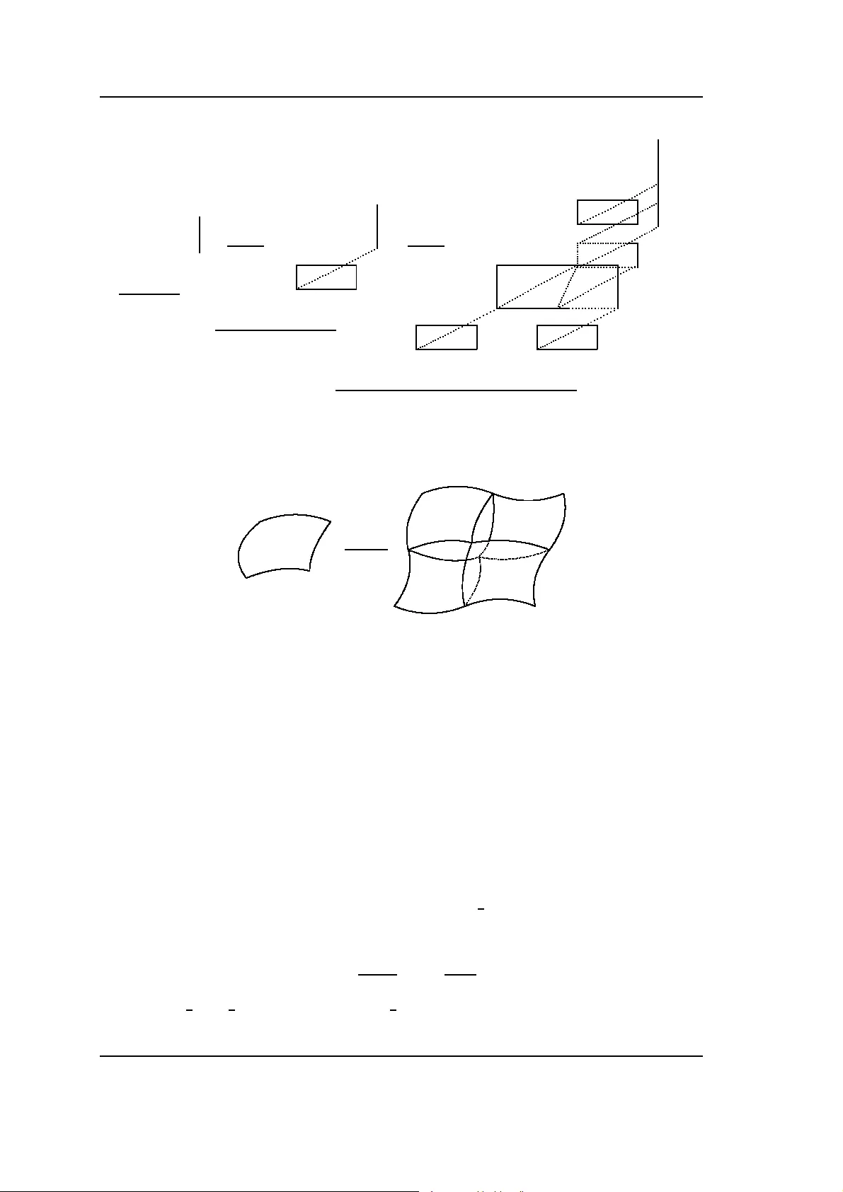
Condensed Matter Phy sics, 2011, V ol. 14, No 1, 13801: 1–18 DOI: 10.5488/CMP .14.13801 http:// www .icm p. lviv .ua/jour nal Motif based hierarc hica l random graphs: structural prope r ties and critical points of an Ising model ∗ Monika K otorowi cz † , Y uri Kozitsky ‡ Institute of Mathematics , Maria Curie-Skłodowska Univ ersity , Lublin, P oland Received March 15, 2010, in final form June 7, 2010 A class of random graphs is i ntroduced and studied. The graphs are constructed i n a n a lgorithmic wa y from fiv e motifs which w ere f ound in [Milo R., Shen-Orr S., Itzk ovitz S ., Kashtan N., Chklovskii D ., Alon U . , Science, 2002, 298 , 824–827]. The construction scheme resemb les that used in [ Hincze wski M. , A. Nihat Berker , Ph ys . Rev . E, 2006, 73 , 066126], according to which the shor t-range bonds are non-random, whereas the lon g-range bonds appear independently with the same probability . A number of structural p roper ties of the graphs hav e been described, am ong which there are degree d istributions, clustering, amenability , small-world p roper ty . For one of the motifs, the critical point of the Ising model defined on the corresponding gr aph has been studied. Key words: amenability , degree distribution, c lustering, small-world graph, Ising model, critical p oint P A CS: 89.75.Fb , 89.75.K d, 05.10.Cc, 05.70.Jk 1. Introduction and setup A v ast v ar iet y of large systems o ccurring in nature and so ciety hav e a very complicated topo log- ical structure. These are the Internet, the W orld Wide W eb, c itation, neural, and so cial netw orks, etc. In view of the complex top ology and unknown or ganizing principles, the netw orks are often mo deled a s random gr aphs. A random graph with a given no de set V is a gra ph in which for a given pair i, j ∈ V , the b ond h i, j i app ears at random. The study of r andom graphs has been orig inated b y P . Erdős and A. Rényi, who were the first to in tro duce such gra phs in [1, 2]. In the Erdős-Rényi random graph model, denoted b y G n,p , the n um ber o f no des is n , and the b onds betw een distinct no des app ear indep enden tly 1 with the sa me pro babilit y p . An imp ortant c haracteristic of a gra ph is the no de de gr e e , which is the n um ber of b onds attached thereat. In G n,p , it is a rando m v a riable, and all such v a riables a re indep endent and hav e the sa me prob a bilit y distribution. Namely , the probability that the degr ee of a given no de is k is given by the Bernoulli law P n ( k ) =  n − 1 k  p k (1 − p ) n − 1 − k , k = 0 , 1 , . . . , n − 1 . (1) F or random g r aphs, the most interesting questions r efer to their asymptotic prop erties in the limit n → + ∞ . T o get nontrivial answers to such questions o ne allows the pa rameters to dep end on n . F or p n = c/ n , the limit of (1) is the Poisson law P ( k ) = c k e − c /k ! , k ∈ N 0 . (2) How ev er, for irregular c omplex netw orks, the random g raph G n,p is no t a go o d mo del since in the mo st of such netw orks the degree distribution is essen tially no n-P oissonian. Many real w orld ∗ This w ork wa s supported by the DFG throug h the pro ject 436 POL 125/0–1 as we ll as through SFB 701: “Sp ektrale Strukturen und T opologische M ethoden in der Mathematik”. Y ur i Koz itsky was also supp orted b y TODEQ MTKD–CT–2005–0300 42. † E-mail: monik a@hektor.umcs.lublin.pl ‡ E-mail: jko zi@hektor.umcs.lublin.pl 1 C.f., ho w ev er, the discussion in [3]. c  M. K otoro wicz, Y u. K ozit sky 13801 -1 M. K otoro wicz, Y u. K ozitsk y net works, e.g. the WWW, are c haracterized b y pow er-law no de degree distributions, which hav e the form P ( k ) = C k − γ , γ > 1 , typical for the so-called sc ale-fr e e graphs. Another imp ortant par ameter c haracterizing a r andom graph is the clustering c o efficient , which is the proba bilit y that t w o no des a re neigh bo rs given they hav e a co mmon neighbor . Clea rly , in G n,p this pr obability is p , and is the sa me indep endently o f whether or not the no des hav e a co m- mon neighbor. Real world net w orks usually ma nifest strong clustering, which once more indicates that Erdős-Rényi type r andom graphs are not appropriate as their mo dels. In [4], D.J. W atts and H. Strogatz prop osed another type o f random graphs, in which the men tioned disadv a n tage is ov ercome. It should b e noted, ho wev er, that such g raphs do not have p ow er law no de degree distri- butions. The next step b eyond the Erdős-Rényi mo del was done by A.-L. Barabá si a nd R. Alb e r t in [5]. In their mo del, the preferenti al attachmen t principle has b een employ ed, t ypical fo r many real netw orks (the Internet, citation and so cia l net w orks). According to this principle, the more connected a no de is, the more likely it receives a new bond. The cons truction o f the Bara bási- Alber t model starts from an initial gr aph with m 0 > 2 no des (neither can b e isolated). At each step, one adds a new no de and connects it to the existing no des. The pro babilit y p i that the new no de is connected to no de i is pro p or tional to the deg ree n i of that no de, that is, p i = n i / ( P j n j ) . Many of the complex netw orks o ccurr ing in nature co ntain characteristic patterns, r ecurring m uch more frequentl y than the other ones. They are ca lled network motifs , see [6 – 11]. Different net works may have different motifs, and motifs in turn can ch aracter ize the netw orks. F or instance, in bio logical reg ulation netw orks it has b een ex perimentally demonstra ted that each of the mo- tifs can perfor m a key information pro cessing function, see [8]. In [10], the authors introduced a random graph mo del based o n some g eometric pr inciples (constraints). Then, they c ompared the app earance of eight elementary three- and four-no de patterns in their model with the same charac- teristics of the Erdős-Rényi r andom graph. It turned out that five of these pa tterns are motifs for their mo del, but not for the Erdő s-Rényi random gra ph, see figure 1 b elow and table 1 in [10]. F or ✡ ✡ ✡ ✡ ❏ ❏ ❏ ❏ ✡ ✡ ✡ ✡ ❏ ❏ ❏ ❏         ❅ ❅ ❅ ❅ Figure 1. Three and four node motifs M 1 , M 2 , M 3 , M 4 , M 5 found in [10]. another random graph mo del, the app earance of the s ame eight patterns was also studied in [1 1]. Note that among these pa tter ns , only M 1 and M 5 corresp ond to complete gra phs (ea c h no de is a neighbor to every other no de). One of the wa ys to get infor ma tion ab out infinite g raphs, also rando m ones, is to study the prop erties of cer tain mo dels of s tatistical physics defined ther eon. The most p opular ones are the Ising and Potts mo dels, as well as the mo dels o f bo nd a nd site p erco lation, see [1 2 ]. On the other hand, in statistical physics certain graphs are employed to mimic a crystal lattice, for which the critical-p oint behavior of the Ising mo del can b e describ ed in an explicit and rigo r ous wa y . T hes e are the so-called hier ar chic al lattic es introduced in [1 3]. Such lattices are defined in a rather algorithmic wa y b y means of the basic pattern, e .g ., by a “diamond”, which is the pa ttern M 3 depicted in figure 1. A mathematical description o f the Gibbs states of the Ising mo del on such graphs was done by P .M. Bleher and E. Žalys in [14, 15]. M. Hinczewski and A. Nihat Berker [16] studied the cr itical- po in t pr oper ties of the Ising mo del o n the diamo nd hier a rchical la ttice ‘decora ted’ by a dditional bo nds, which a ppear at ra ndom. In the pr esent pap er, w e follow the wa y sug gested in [16] and in tro duce hierarchical graphs co ns tructed b y means of the motifs shown in figure 1, decorated b y a dditiona l b onds whic h appear at random and re p eat, in a way , the cor r esp o nding motif. W e analyse some of their characteristics, such a s the av erage deg ree, the no de degree distribution, amenability , the s mall-world prop erty , as w ell as the cr itical-po in t pr oper ties of the Ising mo del. This study o f ours is a co ntin uation of [17], where the gr a ph based on M 1 was int ro duced by one of us. Note that o ur hierarchical g raphs also found applications in cryptog raphy , see [18]. 13801 -2 Motif based hierarchical random g raph 2. The graphs: construction and structural properties 2.1. The construction: informal description As is t ypical for hiera rchical gra phs, e.g ., for hiera rchical lattices in [13, 16], the construction is carried o ut in an algor ithmic wa y: at k -th level, k ∈ N , one pro duces a subgra ph, say Λ k , whic h is then used as a construction element for pro ducing Λ k +1 . The pro cedure is the same at each level, and the star ting element is obtained fro m the corres ponding motif. Let us illustrate this for the simplest case based on the motif M 1 . First we lab el the no des of M 1 b y a , b , and c , as it is shown in figur e 2, and o btain Λ 1 — the triangle. T hen we take three such gr aphs and lab el them by the same lab els. As a result, ea c h of the triangles has no des of tw o kinds: one no de the lab el of whic h coincides with the triangle lab el (e.g., no de a in triangle a ), and tw o no des with no n-coinciding lab els. Thereafter, the tria ngles are glued up according to the follo wing r ule: no de c of tria ngle a is glued up with no de a of triangle c , ect. The no des with the coinciding lab els remain un touched. These are the so-ca lled ex ternal no des of Λ 2 . The r emaining no des ar e c alled internal . The bo nds of the initial tria ngles turn into the b onds o f Λ 2 . W e call them b asi c b onds; they are depicted by solid lines . At the next stag e of the first step, we add the b onds co nnecting the externa l no des in the s a me way as it is in the motif M 1 . Such b onds are depicted by dotted lines and are called de c or ations . As a result, we obtain the gr aph Λ 2 , which has six ba s ic bo nds and three decorations , three external and three internal no des. Then we rep eat the s ame pro cedure — take three copies of Λ 2 , lab el them b y a , b , and c , and divide their ex ternal nine no des into t wo g roups: three no des with coinciding lab els and six no des with non-co inciding lab els. Then the graphs Λ 2 are g lued up as describ ed above. Thereafter, three deco rating b onds are drawn to connect the external no des. This pro cedure is rep eated ad infinitum. Similar cons tructions for motifs M 2 and M 3 are present ed in figure 3 and figure 4, respec tively . Her e w e hav e omitted the decorating b onds not to ov erload the pictures . The picture for M 4 is obtained fro m that for M 3 b y adding the diago nals. The picture for M 5 is just the three-dimensional version of the picture for M 1 , where the basic pattern is a tetrahedron. 2.2. Definitions In o r der to fix the terminology and to make the construction of our graphs mathematically immaculate, we b egin b y introducing a num ber of relev an t mathematical notions. A (simple) gr a ph G is a pair o f sets ( V , E ) , where V is the set o f no des, whereas E is a subset of the Cartesia n pr o duct V × V . W e supp ose that E is symmetric a nd irr eflexive, i.e., h j, i i ∈ E whenever h i, j i ∈ E , a nd h i, i i / ∈ E for every i , j ∈ V . W e say that i and j are co nnected by a b ond if h i, j i ∈ E . In this ca se, we write i ∼ j and s ay that i and j are adjac ent o r that they are neighb ors . Hence, the elements of E themselves can b e ca lled b onds. The g raph is s aid to b e c omplete if each tw o no des are a djacen t. F or a given i , b y n ( i ) we denote the de gr e e of i — the n um ber of its neighbor s. If V is finite, then E is a lso finite, a nd the g raph is said to b e finite. O therwise, the gra ph is infinite. An infinite gra ph is called lo c al ly finite , if n ( i ) is finite for every no de. All the infinite graphs we study are c ountable , which means that bo th sets V and E ar e infinite and countable. Given G = ( V , E ) and G ′ = ( V ′ , E ′ ) , let φ : V → V ′ be such that φ ( i ) ∼ φ ( j ) whenever i ∼ j . Suc h a map φ is called a morphi sm . A bijectiv e morphism is called an isomorph ism . If φ is an isomo rphism, then its inv erse φ − 1 is als o an iso morphism, and then the gra phs G and G ′ are said to be mutu ally isomorphic. Such gr aphs hav e identical s tructures and th us can b e iden tified. In this case, w e also sa y that G ′ is a c opy of G . One observes that this refers to b oth finite and infinite gr aphs. An is omorphism φ : V → V , i.e. which maps the graph onto itself, is called an aut omorphism . T he gra ph G ′ = ( V ′ , E ′ ) such that V ′ ⊂ V a nd E ′ ⊂ E is said to b e a su b gr aph of G = ( V , E ) . In this case, we wr ite G ′ ⊂ G . Supp ose that a subgraph G ′ ⊂ G has a copy , say e G , that is, there exists a n isomor phism φ : e G → G ′ . Then φ , considered a s a ma p φ : e G → G , is called a n emb e dding o f e G into G , wher e a s G ′ is called the image of e G under this embedding. Figur e 1 presents the so-called unlab ele d gra phs, which we call patterns. After lab eling, i.e., attaching a labe l to e a ch of the no des, such a pattern turns into a graph. Another lab e ling may or may not yield the sa me gr a ph. This dep ends on whether or not 13801 -3 M. K otoro wicz, Y u. K ozitsk y there exists the c o rresp onding automorphism. F or instance, a n y lab eling of the triangle M 1 yields the same gra ph since in a n y cas e each of the no des ha s the same n eighbors. F or the pattern M 2 , the left-hand g raph in figur e 3 with the interc hanged lab els a and b is the same. How ev er, the graph with the interc hanges c and d is no t the same anymore. Of course, this new graph is iso morphic to the initial o ne. This is b ecause there is o nly one nont rivial auto mo rphism of M 2 : the one whic h in terchanges a and b , and pre s erves c a nd d . The triangle has six a utomorphisms. Let us now turn to r andom graphs. T o intro duce such a gra ph we need an underlying gr aph G = ( V , E ) a nd a family E of subsets of E . If G is finite, as E o ne can tak e the set of all subsets of E . In the sequel, we deal with such gr aphs only . Thus, for E ′ ∈ E , we say that E ′ has been pick ed at r ando m with pr obability P ( E ′ ) . In the Erdő s -Rén yi mo del G n,p , the underlying g raph is complete with the no de set V = { 1 , . . . , n } . In this mo del, P ( E ′ ) = p | E ′ | , where p ∈ [0 , 1] and | E ′ | stands for the n um ber of elements in E ′ . In other words, the element s of E ar e b eing pick ed independently , each with the s ame pro babilit y p . In a bit complicated mo del, the b onds a r e pick ed independently but with probability whic h dep ends on the b ond. In this ca se, as well as in the case of the Erdős-Rényi mo del, we deal with a random gra ph with indep endent b onds. F or such gra phs, P ( E ′ ) = Y e ∈ E ′ p ( e ) , (3) where p ( e ) is the pr obability of pic king b ond e . The set of g raphs G ′ = ( V , E ′ ) with E ′ ∈ E is called the graph ensemble — each G ′ is pick ed at random from this ensemble. A r andom gr aph mo del is the pair consisting of the graph ensemble and of the function P : E → [0 , 1] . If the function P is as in (3), the graph is said to be a rando m graph with indep endent bo nds. Supp ose that we hav e t wo r andom graph models with indep endent b onds. Let also G = ( V , E ) and e G = ( e V , e E ) be their underlying gra phs a nd φ : V → e V b e a morphism. Then this map is said to be the morphism of the r a ndom gr aphs if for every h i, j i ∈ E , the probability (in the first mo del) that this b ond is pic ked is the s ame as the corr espo nding proba bilit y (in the second mo del) for the b ond h φ ( i ) , φ ( j ) i . 2.3. The construction As was men tioned above, each of our gr a phs is constructed in a n algorithmic wa y fro m the cor- resp onding motif presented in figure 1. Since they are going to b e random graphs with independent bo nds, we hav e to construct the cor resp onding underlying graphs and, to define, for a given bo nd, the pr obability of being pick ed, c.f. (3). In all our models, the bo nds will be of tw o kinds, which we call basic bonds and decorations. Basic bo nds are going to be non-random, i.e. they are pick ed with probability one. Decorating bo nds app ear with probability p ∈ [0 , 1] , which is a para meter of the mo del. T urn now to the construction o f the underlying gra phs. Let q b e the num ber of no des in the cor r esp o nding motif, that is, q = 3 for M 1 and q = 4 for the r emaining motifs. At s tep k = 1 , w e just label the vertices o f the co rresp onding motif by i = 1 , . . . , q and obtain the initial graph Λ 1 = ( V 1 , E 1 ) . All its b onds a re set to be ba s ic. Supp ose now that we have q + 1 co pies of Λ 1 obtained by the iso morphisms φ j 2 , j = 0 , 1 , . . . , q . Thus, in j -th copy the no des are φ j 2 ( i ) , i = 1 , . . . , q . The g raph Λ 2 is o btained from these copies under the following conditions φ 0 2 ( i ) = φ i 2 ( i ) , i = 1 , . . . , q ; φ i 2 ( j ) = φ j 2 ( i ) , i = 1 , . . . , q , i 6 = j. (4) Thu s, the images o f V 1 under φ i 2 and φ j 2 with i 6 = j in tersect only at o ne no de where (4) holds. The maps φ j 2 , j = 0 , 1 , . . . , q embed Λ 1 in to Λ 2 . The nodes φ i 2 ( i ) , i = 1 , . . . , q , are called the external no des of Λ 2 . All other nodes a re ca lled internal . Thus, Λ 2 has q e xternal a nd q ( q − 1) / 2 internal no des. A t this stage, we la bel them b y i = 1 , . . . , q ( q + 1) / 2 in such a w ay that the externa l no des hav e the same lab els as in Λ 1 , that is, φ i 2 ( i ) = i , i = 1 , . . . q . By co nstruction, the b onds obtained as images under the map φ 0 2 are deco rations: they are of the form h φ 0 2 ( i ) , φ 0 2 ( j ) i where i and j are adjace nt in Λ 1 . F rom the first co ndition in (4 ) we see that the decorating b onds connect the external no des of Λ 2 . The re ma ining bo nds of Λ 2 are set to be basic. Now we construct Λ 3 from one co p y of Λ 1 and q copies of Λ 2 . L et φ 0 3 be the map which pro duces the copy of Λ 1 and φ j 3 , 13801 -4 Motif based hierarchical random g raph j = 1 , . . . , q b e the maps which pro duce the copies o f Λ 2 . W e then imp ose the conditions φ 0 3 ( i ) = φ i 3 ( i ) , i = 1 , . . . , q ; φ i 3 ( j ) = φ j 3 ( i ) , i = 1 , . . . , q , i 6 = j (5) and obtain Λ 3 . Thus, φ 0 3 embeds Λ 1 → Λ 3 , and φ i 3 : Λ 2 → Λ 3 , i = 1 , 2 , . . . , q . As ab ov e, the no des φ i 3 ( i ) are set to b e externa l, and the r emaining no des are internal. The ima g es of V 2 under φ i 3 and φ j 3 with i 6 = j intersect only a t o ne no de where (5) holds. Again we lab el the no des of Λ 3 in such a wa y that φ i 3 ( i ) = i , i = 1 , . . . , q . Now let us establish which b onds of Λ 2 are deco rating a nd which are basic. As above, the bo nds co nnecting the externa l nodes a re decor ating. The images of decorating b onds of Λ 2 are decorating b onds in Λ 3 ; the same is also true for the basic b onds — the basic b onds of Λ 3 are exa ctly the images o f the basic b onds of Λ 2 . F or k > 4 , the co nstruction of Λ k from Λ k − 1 and Λ 1 is identical to the constructio n of Λ 3 just describ ed. As above, by V k and E k we denote the sets of no des a nd bo nds of Λ k , resp ectively . Thus, for k > 2 we ha ve E k = E ′ k ∪ E ′′ k , where E ′ k (resp ectiv ely , E ′′ k ) consists of bas ic (resp ectively , decor a ting) b onds. All Λ k , k ∈ N , are considered as subgraphs of an infinite graph Λ ∞ , the s tr ucture and pro perties of which are not impo r tant for the study presented in this ar ticle. Note that the construction principle used ab ov e essentially differs from that used in the con- struction o f the hierarchical lattices in [1 3 – 1 6]. Namely , in our case to o btain Λ k one replaces ea c h no d e of the basic pattern b y a cop y of the g r aph Λ k − 1 . In the hierarchical lattices, one replaces a b ond . As we shall see in the s equel, this leads to essentially differ en t pr op e r ties of the resulting graphs. Below in figure 2, w e illustrate the construction describ ed ab ov e for the case where the basic pa ttern is the motif M 1 . In this case , the bare graph (i.e. the one whic h occur s for p = 0 ) is the approximating gra ph fo r the fra ctal known as the Sierpiński gasket 2 . T he elements of E ′ 2 (middle g raph) a nd of E ′ 3 (right-hand graph) a re depicted by solid lines. The elements of E ′′ 2 and of E ′′ 3 are depicted by dotted lines. W e omit s o me dotted lines to indica te that they app ear a t random and hence may b e absent in a given realization of the gra ph. Note that Λ 3 can b e viewed as the triangle co mpose d of three copies o f Λ 2 . In figure 3, we present the cons tr uction of the bare gr a ph Λ 3 corresp onding to M 2 . In contrast to the former ca se, this is not a planar gr aph. In figure 4, w e construct the bare graph Λ 2 for the motif M 3 . One observes that in that picture the no de c of the low er left-hand quadra t (i.e. quadrat a ) is glued up with no de a of the uppe r right-hand quadrat. It is interesting that the corresp onding fra ctal can b e obtained b y the following pro cedure, resembling the one which yields the Sierpiński g asket. One takes the full quadrat and cuts it out in to four eq ual quadrats, but without cutting the external lines. Then, one g lues up the vertices of the smaller quadra ts as depicted and pro ceeds with cutting out the smaller qua drats. The fractal which one obtains fr o m M 5 is a three dimensional version o f the Sierpiński gasket. O ne takes the full tetrahedro n a nd cuts out its inner o ne fourth in such a wa y that the remaining four tetrahedra are glued up acco rding to the r ule: vertex b of tetrahedro n a is glued up with vertex a of tetrahedron b , etc. ✡ ✡ ✡ ❏ ❏ ❏ a b c ✲ ✡ ✡ ✡ ❏ ❏ ❏ ✡ ✡ ✡ ❏ ❏ ❏ ✡ ✡ ✡ ❏ ❏ ❏ a b γ c β α ✲ ✡ ✡ ✡ ❏ ❏ ❏ ✡ ✡ ✡ ❏ ❏ ❏ ✡ ✡ ✡ ❏ ❏ ❏ ✡ ✡ ✡ ❏ ❏ ❏ ✡ ✡ ✡ ❏ ❏ ❏ ✡ ✡ ✡ ❏ ❏ ❏ ✡ ✡ ✡ ❏ ❏ ❏ ✡ ✡ ✡ ❏ ❏ ❏ ✡ ✡ ✡ ❏ ❏ ❏ a b c Figure 2. Construction of the graph Λ 3 based on M 1 . 2 The fractal i tself i s obtained as the closure of the set ∪ k ∈ N V k in the appropr iate top ology , see e.g. [19]. 13801 -5 M. K otoro wicz, Y u. K ozitsk y ✟ ✟ ✟ ✟ ✟ ✟ ✁ ✁ ✁ a b c d ✲ ✟ ✟ ✟ ✟ ✟ ✟ ✁ ✁ ✁ ✟ ✟ ✟ ✟ ✟ ✟ ✁ ✁ ✁ ✁ ✁ ✁ ✟ ✟ ✟ ✟ ✟ ✟ ✁ ✁ ✁ a b c d ✲ a ✟ ✟ ✟ ✟ ✟ ✟ ✁ ✁ ✁ ✟ ✟ ✟ ✟ ✟ ✟ ✁ ✁ ✁ ✁ ✁ ✁ ✟ ✟ ✟ ✟ ✟ ✟ ✁ ✁ ✁ α b ✟ ✟ ✟ ✟ ✟ ✟ ✁ ✁ ✁ ✟ ✟ ✟ ✟ ✟ ✟ ✁ ✁ ✁ ✁ ✁ ✁ ✟ ✟ ✟ ✟ ✟ ✟ ✁ ✁ ✁ β γ c ✁ ✁ ✁ ✁ ✁ ✁ ✁ ✁ ✁ δ ǫ ζ d ✟ ✟ ✟ ✟ ✟ ✟ ✁ ✁ ✁ ✟ ✟ ✟ ✟ ✟ ✟ ✁ ✁ ✁ ✁ ✁ ✁ ✟ ✟ ✟ ✟ ✟ ✟ ✁ ✁ ✁ Figure 3. Construction of the b are graph Λ 3 based on M 2 . d c a b ✲ d c a b Figure 4. Construction of t h e b are graph Λ 2 based on M 3 . 2.4. Degree distribution Now we turn to the description of the structural prop erties of the graphs constructed ab ov e. Let m k , k ∈ N , b e the num ber o f times the basic pattern app ears in non-decor ated Λ k as a subgr aph. F or the g raphs based on M 1 and M 5 we hav e the s ame situation. Here m 1 = 1 and m k = q m k − 1 , for k > 2 with the exception in Λ 2 , where the additional pattern a ppea rs. So, for M 1 and M 5 we obtain m 1 = 1 and m k = ( q + 1 ) q k − 2 , k > 2 . (6) Here q = 3 a nd q = 4 for M 1 and M 5 , res pectively . F o r motif M 3 we hav e m 1 = 1 , m 2 = 2 q and m k = q m k − 1 , k > 3 . (7) Hence m k = 2 · 4 k − 1 for k > 2 . The simplest case if for M 4 , w her e m k = q m k − 1 for k > 2 . It gives m 4 = 4 k − 1 . The last motif is M 2 – triangle with additional bond. On e a ch level this b ond “pro duces” new 17 pa tterns. So m 1 = 1 and for k > 2 m k = 1 3 (26 · 4 k − 1 − 17) . Now we analyze the num ber of times the basic pattern app ears in fully decorated Λ k , denoted b y e m k . F or the gra phs ba sed on M 1 and M 5 we have e m k = 2 q + 1 q − 1 q k − 1 + q + 2 q − 1 . (8) F or M 3 it is 2 3 4 k − 5 3 and fo r M 4 we obtain 1 3 (4 k − 1) . In all cases, we have m k increasing as C ( p ) q k − 1 , which means that adding decor ations do es not ch ange the a symptotics of m k . 13801 -6 Motif based hierarchical random g raph In a similar way , we obtain | V k | = q k + q 2 , | E k | = r q k − 1 + rp q k − 1 − 1 q − 1 , k ∈ N , (9) where | V k | stands for the num ber of no des in Λ k , whereas | E k | is the exp ected num b er of b onds in this g r aph. As was mentioned ab ov e, the degr ee distribution is a very imp ortant characteristic of the gr aph. In c o n trast to Erdős-Rényi type graphs, fo r our graphs the distribution of the random v ariable n ( i ) depends on the t yp e of i . Thu s, the simplest wa y to describ e this distribution is to av erage n ( i ) ov er the no des of a g iven Λ k , that is, to co nsider n k = 1 | V k | X i ∈ V k n ( i ) . (10) Let h n k i b e the exp ected v alue of n k . Then h n k i = 2 | E k | / | V k | = 4 r q ( q − 1) ( q − 1 + p ) − 4 r q ( q − 1) · q − 1 + 2 p q k − 1 + 1 . (11) How ev er, this result provides only partial information on the no de degree distribution. T o ge t mo re, let us ana lyze the structure of the no de se ts V k , k = 1 , 2 , . . . , mor e in detail. F or a given Λ k and l = 1 , . . . , k , let V ( l ) k be the set of no des i ∈ V k which are external for some Λ l and, at the same time, are in ternal for any Λ l +1 . Of co urse, here we mea n those Λ l ’s which are subgra phs for Λ k . As an example, let us consider the graph Λ 2 based on M 1 , see the middle g raph in figure 2. The no des a , b , and c constitute V (2) 2 , where a s the remaining no des constitute V (1) 2 . The element s of V ( k − 1) k are exactly the no des at whic h the subg raphs Λ j k − 1 , j = 1 , . . . , q are glued up to form Λ k , w her eas the elements of V ( k ) k are exac tly the exter na l no des of Λ k . Then | V ( k ) k | = q and | V ( k − 1) k | = q ( q − 1) / 2 . F or l < k − 1 , we hav e | V ( l ) k | = q | V ( l ) k − 1 | , which can b e so lv ed to yield | V ( l ) k | = 1 2 q k − l ( q − 1) , l = 1 , . . . , k − 1 , | V ( k ) k | = q . (12) The reason to consider the sets V ( l ) k is that all the elements o f each such V ( l ) k hav e the same degree distribution, independent of k for l 6 k − 1 . In fact, the degrees of i ∈ V (1) k are non-r andom since these no des receive no decor ating b onds. F or suc h i , n ( i ) = P j n (0) ( j ) , wher e n (0) ( j ) is the degree of the corresp onding no de in the basic pattern, and the sum is taken ov er all such patterns which a re glued up. By the symmetry of M 1 , M 3 , and M 5 , we hav e n ( i ) = 4 for M 1 and M 3 , and n ( i ) = 6 for M 5 . F o r M 2 , n ( i ) takes v alues 3 , 4 , 5 , see figure 3. F or i ∈ V ( l ) k , l = 2 , 3 , . . . , k − 1 , we hav e n ( i ) = ˜ n ( i ) + ν ( i ) , where ˜ n ( i ) is non-ra ndom and has to b e calculated as just descr ibed. The summand ν ( i ) is the num ber of deco rating b onds a ttac hed to i . T o simplify our considera tion, let us stic k to the case of the gra ph genera ted by M 1 . Then for l = 1 , . . . , k − 1 and i ∈ V ( l ) k , w e ha ve ˜ n ( i ) = 4 and ν ( i ) takes v alues ν = 0 , 1 , 2 , . . . , 4( l − 1 ) , with probability Prob ( ν ( i ) = ν ) =  4( l − 1) ν  p ν (1 − p ) 4( l − 1) − ν . (13) F or i ∈ V ( k ) k , ν ( i ) takes v alues 0 , 1 , . . . , 2( k − 1) . Ther efore, the ma xim um no de deg ree which can o ccur in V k , k > 2 , is max i ∈ V k n ( i ) = 4 k − 4 . (14) As is usual in the theory of real world netw orks, whic h are in fact non-random, the randomness manifests itself as the random c hoice of a no de. If we a pply this principle her e, then (13) can be considered as the conditional pr obability distribution, co nditioned by the even t that the no de i 13801 -7 M. K otoro wicz, Y u. K ozitsk y has been pick ed from the set V ( l ) k . The pro babilit y of the latter even t is taken to be propo rtional to the num ber of its elements, that is, Prob  i ∈ V ( l ) k  = | V ( l ) k | | V k | = q − 1 1 + q 1 − k q − l = 2 1 + 3 1 − k 3 − l , l 6 k − 1 , (15) Prob  i ∈ V ( k ) k  = 2 q q k + q = 2 3 k − 1 + 1 . If we now take the exp ectation of n ( i ) with res pect to this distribution, that is, h n k i = k − 1 X l =1 4( l − 1) X ν =0 (4 + ν ) 2 · 3 − l 1 + 3 1 − k ·  4( l − 1 ) ν  p ν (1 − p ) 4( l − 1) − ν (16) + 2( k − 1) X ν =0 (2 + ν ) 2 3 k − 1 + 1 ·  2( k − 1) ν  p ν (1 − p ) 2( k − 1) − ν , we r e a dily obtain h n k i = 4 + 2 p − 4(1 + p ) / (3 k − 1 + 1) , whic h is in full agre emen t with the one given in (11) or in table 1. In o rder to figure out the limit k → + ∞ of the distribution given by (13 ) and (15) we calculate its characteristic function, c.f. (16), ϕ k ( t ) = k − 1 X l =1 4( l − 1) X ν =0 exp [i t (4 + ν )] 2 · 3 − l 1 + 3 1 − k ·  4( l − 1 ) ν  p ν (1 − p ) 4( l − 1) − ν (17) + 2( k − 1) X ν =0 exp [i t (2 + ν )] 2 3 k − 1 + 1 ·  2( k − 1) ν  p ν (1 − p ) 2( l − 1) − ν = 2 e 4i t 1 + 3 1 − k · 1 − 3 1 − k  e i t p + 1 − p  4 3 − ( e i t p + 1 − p ) 4 + 2 e 2i t 3 k − 1 + 1  e i t p + 1 − p  2 , i = √ − 1 . Then the limiting characteristic function is ϕ ( t ) = 2 e 4i t 3 − ( e i t p + 1 − p ) 4 , (18) which can b e contin ued to a meromorphic function analytic in some complex neighbor hoo d of the point t = 0 . T his means that the limitin g no de degr e e distribution has all momen ts and hence canno t b e of scale-free type 3 . This also ag rees with the heuristic rule, see equation (3.13) on page 188 in [20], that for scale-free netw orks max i ∈ V k n ( i ) ∼ | V k | 1 / ( α − 1) , α > 1 , (19) whereas in o ur ca s e we have (14) and | V k | = (3 k + 3) / 2 . In a similar way , one ca n s ho w that all our g raphs a re not scale-free. Another obser v ation on this item ca n b e made by comparing the function (18) with the ch aracteris tic function o f the Poisson distribution (2) which has the form ϕ Poisson ( t ) = exp  c  e i t − 1  , and hence ca n b e contin ued to a function a nalytic on the whole co mplex plane. There fo r e, the distribution co rresp onding to (18) with p > 0 is intermediate as compare d to the Poisson and scale-free distributions. F or p = 0 , the function (18) is also ent ire. 3 F or scale-free graphs, the node degree distribution is P ( k ) = C k − γ , k > 1 , γ > 1 ; hence, P ∞ k =1 k m P ( k ) diverg es for all m > γ − 1 . 13801 -8 Motif based hierarchical random g raph 2.5. Amenability , cl ustering, and small world pr operties The next pr ope rt y of our graphs which we ar e g oing to a ddress is amenability . T o introduce it we need one more notion. Let G = ( V , E ) b e a countable gr aph with no de set V and b ond set E . F or a finite ∆ ⊂ V , by ∂ ∆ w e denote the set of no des whic h are not in ∆ but have neighbo r s in ∆ . This set is the outer b oundary o f ∆ , whereas the elemen ts o f ∆ which are neighbors to the elements of ∂ ∆ constitute the inner b oundary of ∆ . As usua l, by | ∆ | and | ∂ ∆ | we denote the num ber o f no des in these sets. The gra ph G is sa id to b e amenable if there exists a s equence of finite no de sets { ∆ k } k ∈ N , such that lim k → + ∞ | ∂ ∆ k | | ∆ k | = 0 . (20) If such a limit is p ositive for any sequence { ∆ k } k ∈ N , the g raph is called nonamenabile . The la ttices Z d , d > 1 , ar e a menable graphs a nd for such sets one can take the cub es ∆ k = { i = ( i 1 , . . . i d ) ∈ Z d : | i j | 6 N k , j = 1 , . . . , d } , such that N k +1 > N k and N k → + ∞ . In this case , | ∆ k | ∼ N d k and | ∂ ∆ k | ∼ N d − 1 k and hence (20) holds. Sometimes, sequences for which (20) holds a r e ca lled V an Howe sequences, see e.g. [21]. Cayley trees, e x cept for Z , ar e nonamenable. Let us turn now to our graphs. Due to their hier archical structure, it is convenien t to chec k (20) for the se q uence of no de sets of Λ k , that is for { V k } k ∈ N . By the construction of Λ k , the inner b oundar y of ea ch V k is exactly the se t of all its ex ter nal no des, the n um ber of which is eq ua l to the num ber of nodes in th e cor r esp o nding motif, i.e. it is q . By co nstruction, one of them b ecomes an external no de o f Λ k +1 , and the rema ining q − 1 ones bec o me inner no des of Λ k +1 . F or all the motifs M j , j = 1 , . . . , 5 , we hav e the degree o f any no de therein b eing a t most 3 , see figure 1. Then for all our gr aphs, max i ∈ V k n ( i ) 6 6 k , c.f. (14). A t the same time, | V k | ∼ q k , q = 3 , 4 , se e (9), which immediately yields that all our graphs are a mena ble. Now we study the clustering in our gr aphs. F or non-r andom gr aphs, the clustering co efficien t is defined as follows. F or a given no de i ∈ V of degr ee n ( i ) , let N ( i ) be the n um ber of bo nds linking its neighbors, whic h is the num ber of triangles with vertex i . Clear ly , N ( i ) 6 n ( i )[ n ( i ) − 1] / 2 and the maximum v alue of this parameter is attained for complete gra phs where each no de is a neighbor to any other one. Thus, the qua n tit y Q ( i ) := 2 N ( i ) n ( i )[ n ( i ) − 1 ] , (21) characterizes cluster ing at no de i . Then we define the clustering of our gr aphs as Q = lim k → + ∞ 1 | V k | X i ∈ V k Q ( i ) . (22) Note that for many graphs, e.g., for trees or bipartite gr aphs, one has Q ( i ) = 0 for any no de i , see a lso [2 2, 2 3]. F or random graphs, the degree n ( i ) , as well as the par ameter N ( i ) , are rando m. Since in this case the ca lcula tion of Q is muc h more in v olved, we p ostp o ne it to the future. Here we only compare the v a lues of Q obtained for the bar e g raphs with those for fully decorated ones. F or the graph base d on M 1 and a no de i ∈ V ( l ) k , l = 1 , . . . , k − 1 , we have: (a) n ( i ) = 4 , N ( i ) = 3 for l = 1 , and N ( i ) = 2 for l > 2 ; (b) n ( i ) = 4 l , N ( i ) = 4 l . Here (a) and (b) corresp ond to a bare graph and to a fully decor ated g raph, resp ectiv ely . These num bers follow directly from the construction of the gr a phs. The num ber of elements in each V ( l ) k is given in (12), which a llows o ne 13801 -9 M. K otoro wicz, Y u. K ozitsk y to compute (a) Q = lim k → + ∞ 1 3 + | V (1) k | 6 | V k | + 2 | V k | ! = 4 9 = 0 . 4444 . . . , (23) (b) Q = 2 · 3 − 1 / 4 arctan 3 − 1 / 4 − 1 3 1 / 4 ln 3 1 / 4 + 1 3 1 / 4 − 1 ≈ 0 . 5 25897 . (24) F or the bare graph ba sed on M 3 , we hav e N ( i ) = 0 for all nodes; hence, Q = 0 in this ca se. F or the fully decorated graph based on M 3 , we o bserve that t wo no des of V (1) 2 hav e neighbor s only in V (1) 2 , and the remaining fo ur no des hav e t wo neighbor s in V (1) 2 and tw o — in V (2) 2 . Since for the no des i ∈ V (1) 2 , we have N ( i ) = 0 , like in the case of the ba re graph, we should co nsider these tw o groups se pa rately . Thus, we split each V ( l ) k , l = 1 , . . . , k − 1 , into V ( l ) k, 0 and V ( l ) k, 1 , where the firs t set consists of the no des which have neighbors only in V ( l ) k, 0 . The e le ments of V ( l ) k, 1 hav e also neig h bo rs in V ( l ′ ) k with l ′ > l . The num ber o f no des in these sets are: | V ( l ) k, 0 | = 1 2 4 k − l , | V ( l ) k, 1 | = 4 k − l . F or all i ∈ V ( l ) k , l = 1 , . . . , k − 1 , we hav e n ( i ) = 4 l . A t the same time, N ( i ) = 4( l − 1) for i ∈ V ( l ) k, 0 , and N ( i ) = 1 + 4( l − 1 ) for i ∈ V ( l ) k, 1 . Putting all these num b ers together we obtain Q = 3 2 ∞ X l =2 ( l − 1)4 − ( l − 1) l (4 l − 1) + ∞ X l =1 4 − l l (4 l − 1) ≈ 0 . 1223 . (25) F or the bare graph based on M 5 one can o btain fo r i ∈ V ( l ) k , l = 1 , 2 , . . . , k − 1 : n ( i ) = 6 , N ( i ) = 8 for l = 1 , a nd n ( i ) = 6 , N ( i ) = 6 for l > 2 . F or the fully deco rated g raph bas ed on M 5 we hav e for all internal nodes n ( i ) = 6 l , a nd N ( i ) = 9 for l = 1 , and N ( i ) = 12 l + 7 for l > 2 . Hence, we o btain (a) Q = lim k → + ∞ 2 5 + 2 | V (1) k | 15 | V k | + 12 5 | V k | ! = 0 . 5 , ( 26) (b) Q ≈ 0 . 5541 45 . There exists one mor e prop erty o f real world netw orks, which Erdős-Rényi type graph do es not share, see e.g. [20, 24]. It is the so-called smal l-world pr op erty , illustrated by P al Erdős himself in the following way . All authors of ma thematical pap ers are given the Er dős index whic h for his coauthors is equal to one. F or their coauthors who are no t Erdő s’ coauthors, this index is equal to 2, and so on. Everyone whos e pap ers a re indexed b y the Mathematical Reviews can check his own index a t the web-site ht tp://www.ams.or g/mathscinet/ . It turns o ut that for many author s it ranges fro m 2 to 6 (for the second named author of this pap er it is 4). T o formulate the small-world prop erty one needs the following notion. A path in the graph is a sequence of nodes such that every t wo c o nsecutive elements o f this sequence are neigh bo rs to each o ther . The length of the path is the num ber of such consecutive pairs, which is equal to the n umber o f b onds one passes o n the wa y from the origin to the terminus. If every tw o no des ca n b e connected by a path, the graph is said to b e connected. F or the giv en t w o nodes, i and j , the length of the shortest path which connects them is said to b e the distance ρ ( i, j ) b et w een these no des. Informally sp eaking, a graph G = ( V , E ) has the small-world pr ope rt y (or is a small-world graph) if every t w o nodes i, j ∈ V are “not to o far” from each o ther. More precis ely this prop erty is formulated as follows. An infinite graph G has a s mall-world proper t y if there exists a seq uence o f its connected finite subgr aphs { G k } k ∈ N with the following prop erty . Let dia m( G k ) = max i,j ∈ V k ρ ( i, j ) b e the dia meter o f G k , k ∈ N , a nd h n k i b e the av erage v alue o f the no de degree in G k , that is, h n k i = 2 | E k | / | V k | . Then 13801 -10 Motif based hierarchical random g raph the sequence { G k } k ∈ N , and hence the g raph G , ar e s aid to hav e the small-world prop erty if there exists a p ositive constant C such that for all k ∈ N , diam( G k ) 6 C log h n k i | V k | . (27) This means that in such graphs, the dis ta nces betw een the no d es scale at most logarithmically with the s ize of the graph. F o r our g raphs, the results on this item are given in the last three rows of table 1. The diameters of Λ k presented therein were c a lculated in a r outine w ay for the cases where the graphs a re bare ( p = 0 ) or are fully decor ated ( p = 1 ). In the former case, neither o f our graphs has the small-world prop erty . How ev er, this pro per ty holds for a ll fully decor ated graphs. T able 1. The structural c haracteristics of the familie s of hierarc hical graphs. motif M 1 M 2 M 3 M 4 M 5 | V k | 3 2 (3 k − 1 + 1) 2(4 k − 1 + 1) 2(4 k − 1 + 1) 2(4 k − 1 + 1) 2(4 k − 1 + 1) | E k | 3 k 4 k 4 k 5 · 4 k − 1 6 · 4 k − 1 3 2 (3 k − 1 − 1) p 4 3 (4 k − 1 − 1) p 4 3 (4 k − 1 − 1) p 5 3 (4 k − 1 − 1) p 2(4 k − 1 − 1) p h n k i 4 + 2 p 4 + 4 3 p 4 + 4 3 p 5 + 5 3 p 6 + 2 p − 4 1+ p 3 k − 1 +1 − 4 3 3+2 p 4 k − 1 +1 − 4 3 3+2 p 4 k − 1 +1 − 5 3 3+2 p 4 k − 1 +1 − 2 3+2 p 4 k − 1 +1 diam(Λ k ) , p = 0 2 k − 1 2 k 2 k 2 k 2 k − 1 diam(Λ k ) , p = 1 k k + 1 2( k − 1) k k C , p = 1 (log 6 3) − 1 (log 6 4) − 1 2(log 6 4) − 1 (log 7 4) − 1 (log 8 4) − 1 In table 1, we collected the structural characteristics of o ur gr aphs based on the mo tifs M 1 , . . . , M 5 given in figure 1. Its firs t three rows are o btained from the formulas (9) and (11). 3. Graph structure and the Ising model properties As w as mentioned a bove, there exists a pr o found connection b e tw een the prop erties of Gibbs random fields of mo dels ba sed o n g raphs and the structura l pr op erties o f these g raphs 4 . F or the hierarchical lattices, the notion of the Gibbs random field o f the Ising mo del was in tro duced in [14, 15]. In the ph ysical terminolog y , each (pure) Gibbs random field cor r esp o nds to a state of thermal e q uilibrium of the mo del, see [2 5] for more details. Accordingly , the existence of multiple Gibbs random fields corresp onds to the existence of mu ltiple equilibrium states and hence of phase transitions. If there is no interaction b et w een the spins, the Gibbs r andom field is unique. How ev er, if the in teraction is strong eno ug h and if it is e ffectively propag a ted b y the underlying gr aph (high enough “connectivity”), the Gibbs fields ca n be m ultiple. The condition of high connectivity is essential, which ca n b e seen from the fact that the Ising mo del o n the o ne-dimensional lattice Z , considered as a g raph with the natura l a djacency rela tion, bear s only one Gibbs field and hence no phase transitions can o c cur in this ca se – no matter how s tr ong the interaction is. With r e g ard to these arg umen ts, we can divide all graphs into three g roups acco rding to the following prop erty of the Is ing mo del defined on these gra phs: 4 Of course, we are speaking now ab out coun tably infinite graphs. 13801 -11 M. K otoro wicz, Y u. K ozitsk y (a) There exists only one Gibbs rando m field for all interactions. (b) There exists only one Gibbs rando m field for weak interactions, and multiple Gibbs random fields for strong interactions. (c) There exist multiple Gibbs r andom fields for all nonzero interactions. As was mentioned ab ov e, the lattice Z b elongs to the first group. The lattices Z d with d > 2 , a s well as all Cayley trees 5 belo ng to the seco nd group. An example of the gr a ph b elonging to the third group can b e found in section 4 of [2 6]. C le a rly , the ab ov e classification should b e made mor e precise for random g r aphs, since in this cas e the exis tence of a Gibbs random field is a ra ndom even t. W e r eturn to this issue b elow. The Ising mo del defined on the gr a phs from the second group may have a critic al p oint , which separates the re gime of uniqueness (weak in teractions) from the regime of non-uniqueness (strong in teractions). A t their critical po in t, the Gibbs random fields ha ve “unusual” pr ope rties, which can be detected without explicit construction of these fields. One of suc h pr oper ties is the so- called self-similari ty , whic h ma nifests itself in the app eara nce of unstable fixe d p oints of some (renormalizatio n) transformations. It turns o ut that the hier archical gr aphs are quite suitable for such a study — that it wh y they app ear in this con text. Thus, o ne can hav e the following criterio n: if the Ising mo del has a cr itical p oint, the graph b elongs to the second gr oup. I f not, then the graph b elongs either to the fir st o r to the third group. The la tter cases can be distinguis hed by an additional study . In contrast to the hierarchical lattices in tro duced and studied in [16], our bare gra phs b elong to the first group. This can b e seen from the a nalysis which we pr esent b elow — a direc t pro of of such a statemen t will be done in our forthcoming publicatio n. Thus, the int eraction alo ng the decorating b onds plays the main role in the pos sible app earance of phase transitions in the Ising mo del defined on our graphs. In view of this fact, we will assume that the solid b onds be a r the in teraction K , whereas the dotted b onds b ear the interaction L . As the b onds of the latter kind app ear at ra ndom, we can think of the corresp onding mo del as o f the o ne defined on the fully decorated graph with ra ndo m in teractions along the deco rating b o nds. Thus, in this mo del, the in teraction alo ng each bo nd h i , j i is a random v ariable, denoted by L ω ij , which takes v alues 0 and some nonzero L ∈ R with pro babilities 1 − p a nd p , resp ectively . F or different b onds, these r a ndom v ar iables are indep enden t. F or a given k ∈ N , the Ising mo del o n the fully decorated gra ph Λ k is defined in the usual wa y b y assig ning s pin v ariables σ i = ± 1 to the no des i ∈ V k and by setting the Hamiltonian − β H k = h X i ∈ V k σ i + K X h i,j i∈ E ′ k σ i σ j + X h i,j i∈ E ′′ k L ω ij σ i σ j , h, K ∈ R , k ∈ N , (28) where h is an external field. In acco rdance with the ab ov e ar g umen ts, the third s umma nd cor- resp onds to the interaction a lo ng decorating b onds. W e have included the first term in view of the following a rguments. As is known, the Ising model on the l attices Z d , d > 2 , exhibits phase transitions only if h = 0 . This is also the case if the gr a ph is amenable and quasi-transitive. F or nonamenable graphs, this mo del may hav e a phase tra nsition for no nzero h , s ee [27]. By the construction of our graphs, ea c h Λ k has q externa l no des, i 1 , . . . , i q , a nd the corresp ond- ing num ber of internal no des, see table 1. Such exter na l no des can b e considered as a b oundary of Λ k . Corr esp o ndingly , we call the spin v ariables external or b oundary (r espectively , internal ) spins if they are ass igned to external (resp ectively , int ernal) no des. F or a fixed configura tion of the external spins σ i 1 , . . . , σ i q , we consider Z ω k ( σ i 1 , . . . , σ i q ) = X internal sp ins of Λ k exp ( − β H k ) . (29) This is the conditional partition function of the spin system in Λ k , conditioned by the fix e d configuration of spins on the b oundary of Λ k . Of course, it depends on the gr aph, i.e. on the motif 5 Except for Z , see page 247 in [25]. 13801 -12 Motif based hierarchical random g raph used in its construction. A ccording to the main principle of the theory of Gibbs ra ndom fields applied in our con text, see [25], the fact that such a field is unique is ensured by the conditional partition function a symptotic independence, as k → + ∞ , of the b oundary spins. F or our graphs, Z ω k are random a nd hence also dep end o n ω . In this situation, o ne ca n apply the following tw o approaches: the ab ov e mentioned indep endence holds (i) for almost all ω ; (ii) in a verage. The latter corresp onds to the fact that the exp ected v a lues of Z ω k , which we denote by h Z ω k i , are indep enden t of the b oundary spins. These tw o appr o aches ar e called quenche d and anne ale d disorders, resp ectively , see [28], page 99. W e will work in the annealed approach. It can b e s hown that the s ummands in (29) are p ositive and separated fro m zero. Since the num ber of these summands increase s to + ∞ a s k → + ∞ , we hav e h Z ω k i → + ∞ . Ther efore, a weak er form of the uniqueness condition can b e lim k → + ∞ h Z ω k ( σ i 1 , . . . , σ i q ) i / h Z ω k ( σ ′ i 1 , . . . , σ ′ i q ) i = c, (30) which holds for any tw o configur ations of the boundar y spins a nd for some c > 0 , whic h dep ends on these config ur ations. The conv ergence in (30) should b e stable with resp ect to small changes of h and K , i.e. o f the starting element Z 1 . In this ca se, the annealed limiting free energy p er spin is independent o f the b oundary co nfiguration. Corresp ondingl y , a necessary condition for the la tter quantit y to be dep endent on the b oundary spins is that lim k → + ∞ h Z ω k ( σ i 1 , . . . , σ i q ) i / h Z ω k ( σ ′ i 1 , . . . , σ ′ i q ) i = + ∞ , (31) for so me σ i 1 , . . . , σ i q and σ ′ i 1 , . . . , σ ′ i q . W e say that the Ising mo del defined o n our graph has a critical p oint, if there exists c ′ > 0 , distinct fro m c in (30), such that for K = K ∗ and h = h ∗ , lim k → + ∞ h Z ω k ( σ i 1 , . . . , σ i q ) i / h Z ω k ( σ ′ i 1 , . . . , σ ′ i q ) i = c ′ . (32) Here K ∗ and h ∗ are certain v a lues of the interaction in tensit y and the external field. The conv er- gence in (32 ) should b e such that for arbitrar ily small dev iations from the p oint ( K ∗ , h ∗ ) one has either (30) or (31 ) instea d of (32). Note that we do not ex c lude that h ∗ 6 = 0 since our gr aphs a re not quasi-tra nsitiv e and hence the result o f [27] may not b e applicable in this cas e. 4. Critical points of the Ising model on M 1 based graph F or k = 1 , we have o nly basic b onds and no inner no des. Thus, Z 1 ( a, b, c ) = exp [ − β H 1 ( a, b, c )] = exp[ K ( ab + ac + bc ) + h ( a + b + c )] , (33) where we use the sa me notations for the no des a, b , c , see the left-hand graph in figure 2, as w ell as for the corr esp o nding spin v ariable, tha t is , for short we wr ite a = σ a , b = σ b , ect. F or k = 2 , we have, see the middle graph in figure 2, − β H 2 ( a, b, c, α, β , γ ) = − β H 1 ( a, γ , β ) − β H 1 ( γ , b, α ) − β H 1 ( β , α, c ) + L ω ab ab + L ω bc bc + L ω ac ac. Thu s, to obtain Z 2 ( a, b, c ) we hav e to sum o ut the internal spins, see (29). That is, Z ω 2 ( a, b, c ) = exp [ L ω ab ab + L ω ac ac + L ω bc bc ] X α,β ,γ Z 1 ( a, γ , β ) Z 1 ( γ , b, α ) Z 1 ( β , α, c ) , where the sum is taken over α, β , γ = ± 1 . According to the hierar c hical structure of the underlying graph, for all k > 2 the graph Λ k is obta ined from the subgraphs Λ k − 1 exactly in the s ame wa y . This yields the following recurrence for the par tition functions (29) Z ω k ( a, b, c ) = R ω k ( a, b, c ) X α,β ,γ Z k − 1 ( a, γ , β ) Z k − 1 ( γ , b, α ) Z k − 1 ( β , α, c ) , (34) 13801 -13 M. K otoro wicz, Y u. K ozitsk y where R ω k ( a, b, c ) = exp [ L ω ab ab + L ω ac ac + L ω bc bc ] , (3 5) and Z 1 ( a, b, c ) is given in (33). F rom the indep endence of L ω ij for differen t bo nds, it follows that the random v a riables Z ω k − 1 on the right-hand side of (34) are indep enden t, which a llows us to co mpute the exp ectations a nd obtain h Z ω k ( a, b, c ) i = h R ω k ( a, b, c ) i X α,β ,γ h Z ω k − 1 ( a, β , γ ) ih Z ω k − 1 ( α, b, γ ) ih Z ω k − 1 ( α, β , c ) i . (36) W e recall that the random v ariables L ω ij take the v alues L 6 = 0 and 0 with probabilities p and 1 − p , resp ectively . In view of the mo del symmetry , c.f. (33), the system (36) inv olves the following v ar iables A k = h Z ω k (1 , 1 , 1) i , B k = h Z ω k (1 , 1 , − 1 ) i , (37) C k = h Z ω k ( − 1 , − 1 , 1) i , D k = h Z ω k ( − 1 , − 1 , − 1) i , which hav e the initial v alues A 1 = e 3( K + h ) , B 1 = e − K + h , C 1 = e − K − h , D 1 = e 3( K − h ) . (38) By direct ca lculations, h R ω k (1 , 1 , 1) i = ( p exp( L ) + 1 − p ) 3 , (39) h R ω k ( − 1 , 1 , 1 ) i = ( p exp( L ) + 1 − p )( p ex p( − L ) + 1 − p ) 2 . Thereafter, the r ecursion (36) can be written in the form x k +1 = t P x ( x k , y k ) Q ( x k , y k , z k ) , (40) y k +1 = P y ( x k , y k , z k ) Q ( x k , y k , z k ) , z k +1 = t P z ( y k , z k ) Q ( x k , y k , z k ) , with the initial conditions x 1 = e 4( K + h ) , y 1 = e 2 h , z 1 = e 4 K − 2 h , (41) where we hav e used the nota tions x k = A k /C k , y k = B k /C k , z k = D k /C k , k ∈ N , (42) and t =  p e L + 1 − p p e − L + 1 − p  2 . (43) The p olynomials in (40) have the fo llowing form P x ( x, y ) = x 3 + 3 xy 2 + 3 y 2 + 1 , (44) P y ( x, y , z ) = x 2 y + y 3 + 2 xy + y 2 z + 2 y + z , P z ( y , z ) = y 3 + 3 y + 3 z + z 3 , Q ( x, y , z ) = xy 2 + x + 2 y 2 + 2 y z + z 2 + 1 . 13801 -14 Motif based hierarchical random g raph F or every t > 0 , the mapping ( x k , y k , z k ) 7→ ( x k +1 , y k +1 , z k +1 ) = T t ( x k , y k , z k ) , defined in (40) and (44), maps the firs t o ctant o f R 3 in to itself. The star ting po in t ( x 1 , y 1 , z 1 ) lies o n the sur fa ce S defined by the equation, c.f. (41), x = y 3 z , (45) which , how ever, is not preserved b y this mapping, which ca n b e chec k ed directly . Let T t be the in v ar iant s et of the map T t , that is, the set of points ( x, y , z ) suc h that T t ( x, y , z ) = ( x, y , z ) . Suppos e that the in tersection of T t with S is no n- v oid. If ( x ∗ , y ∗ , z ∗ ) b elongs to this intersection and ( x 1 , y 1 , z 1 ) = ( x ∗ , y ∗ , z ∗ ) , then ( x k , y k , z k ) = ( x ∗ , y ∗ , z ∗ ) for all k ∈ N . Let us find such po in ts. F rom the s e c o nd equation in (40) for x = y 3 z w e get y Q ( y 3 z , y , z ) = P y ( y 3 z , y , z ) , which can be transfo r med int o the following y 3 (1 + y 3 z )(1 − y z ) = ( y + z )(1 − y z ) . (46) A s olution of the latter equation is z = 1 / y , thus x = y 2 , which b eing used in the first equation in (40) yields (1 + y 2 ) 2 = t (1 + y 2 ) 2 and hence t = 1 . F or p > 0 , the latter implies L = 0 , and a lso K = 0 , see (41). This fixed p o in t c o rresp onds to a noninteracting s ystem o f spins in an external field and thereby has nothing to do with critical p oints. F or z 6 = 1 /y , from (46) we get z (1 − y 2 )( y 4 + y 2 + 1) = − y (1 − y 2 ) , (47) which for positive y and z has a unique solution y = 1 , and hence x = z . W e insert this into the first equation in (40) and obtain x = t x 3 + 3 x + 4 x 2 + 4 x + 3 = t x 2 − x + 4 x + 3 := φ t ( x ) . (48) F or t = 1 , the only solution is x = 1 , which corre s ponds to L = K = 0 . The choice t = 1 als o corresp onds to a bare graph ( p = 0 ); hence, the bare g raph base d on M 1 has no critical p oin ts and no phase trans itions. As we hav e alrea dy ment ioned a bove, in a sepa rate work we prov e that the Gibbs states of the Ising model bas ed on this g raph a re a lwa ys unique. F or t < 1 , that is, for L < 0 , (48) has only o ne p o sitive solution x ∗ = − 3 − t + √ 9 + 22 t − 15 t 2 2(1 − t ) < 1 , (49) which corr espo nds to K ∗ < 0 . It is stable and ( x k , y k , z k ) → ( x ∗ , 1 , x ∗ ) as k → + ∞ , for any ( x 1 , y 1 , z 1 ) ∈ S . Thus, for L < 0 , the Ising mo del has no critica l p oints and no phas e trans itio ns, even for the fully decorated graph. This c a n b e ca us ed by a frustration, whic h tak es place in an antif erromag netic Ising mo del on triangles. F or t > 1 , figur e 5 presents the gra phical s olutions of (48). They hav e the following form x (1) ∗ = 3 + t − √ 9 + 22 t − 15 t 2 2( t − 1) , x (2) ∗ = 3 + t + √ 9 + 22 t − 15 t 2 2( t − 1 ) . (50) By direct ca lc ula tions, we get φ ′ t ( x (1) ∗ ) < 1 and φ ′ t ( x (2) ∗ ) > 1 , see fig ure 5. Hence, x (1) ∗ is stable, whereas x (2) ∗ is unstable. Note a lso that x (1) ∗ → 1 and x (2) ∗ → ∞ as t → 1 . The solutions (5 0) ex ist and are considered to b e distinct, provided t ∈ (1 , 9 / 5 ) . This yields the condition p < ψ ( L ) := 3 − √ 5 √ 5 exp( L ) − 3 exp( − L ) + 3 − √ 5 . (51) Since ψ ( L ) is a decreas ing function, the e quation ψ ( L ) = 1 has only one solution L ∗ = 1 4 ln 9 5 . (52) 13801 -15 M. K otoro wicz, Y u. K ozitsk y ✲ ✻            4 3 t x (1) ∗ x (2) ∗ φ t ( x ) Figure 5. Graphical solution of (48). Then, for L 6 L ∗ , the critica l po in t e xists for all p ∈ (0 , 1] . F or such L and p , let K ∗ ( L, p ) be the solution of the equation exp(4 K ) = x (2) ∗ . (53) Then lim k → + ∞ x k =        x (1) ∗ if x 1 < exp[4 K ∗ ( L, p )] , x (2) ∗ if x 1 = exp[4 K ∗ ( L, p )] , + ∞ if x 1 > exp[4 K ∗ ( L, p )] . (54) The conditions in (5 4) can b e formulated dir e c tly for K , e.g . x k → x (1) ∗ if K < K ∗ ( L, p ) . Thus, x (1) ∗ is the so-called high- temp eratur e fixed p oint. F or L > L ∗ , we hav e ψ ( L ) < 1 . Hence, the condition (51) is not satisfied for p ∈ ( ψ ( L ) , 1] , which also includes the fully deco r ated graph w ith p = 1 . F or such L and p , the whole gra ph of φ t lies above the line φ t ( x ) = x , whic h means that x k → + ∞ for all initial x 1 > 0 . Th us, for L > L ∗ and p ∈ ( ψ ( L ∗ ) , 1] , the mo del has no critica l po in ts a nd the Gibbs random fields are multiple fo r all K ∈ R . F or p = ψ ( L ∗ ) , w e ha ve t = 9 / 5 and x (1) ∗ = x (2) ∗ = 3 , whic h corresp onds to K ∗ = (ln 3) / 4 . In this cas e, x k → 3 if K 6 K ∗ , and x k → + ∞ if K > K ∗ . 5. Conc luding remarks 5.1. Construction and structural properties The graphs introduced in this pa p er are constructed from motifs M 1 , . . . , M 5 in an algo r ithmic wa y , lik e the hierarchical lattices in tro duced in [1 3], and employed in [16] where they w ere supplied with lo ng-range (deco rating) b onds. How ev er, our main construction principle — to replace no des with the g r aphs of the previous lev el — differs from the one use d in thos e pa p ers , where the g raphs of the previous level repla c e d the b onds. Hierarchical g raphs of this kind mo del the real world net works with the so-ca lled mo dula r structure, which ar e orga nized in tightly knit communities with relativ ely spa rse connections b etw een them. F or more details herein, we refer the reader to [29, 3 0] and to the publications cited therein. In contrast to the gra phs introduced in [16], see also [29], our decorated graphs are not scale-free. F or them, the node degr ee distribution is o f in termediate type such that a ll the moments exist. The corr espo nding characteristic function ca n be extended to a meromorphic function, a nalytic in the complex neigh bor ho od of zero, see (18), whereas for scale-free graphs such functions a re nonanalytic at zero. All our g raphs a re amenable, which cor relates with the pro p erty just discussed, see (14), (9), and (1 9). An interesting prop ert y is that, like for the gra phs studied in [16], a dding decora tions forms the graphs p osses sing the small-world prop erty . 13801 -16 Motif based hierarchical random g raph 5.2. Critical points The app earance of c r itical points, and hence of phase transi tions, for the Ising mo del confirms go o d communicating pr ope r ties of the underlying g raphs. F or our graphs, in con trast to the hiera r - chical lattices for which phase tr ansitions ta k e place even without deco r ations, critical p oints can exist only if the decora tions are applied, with any p > 0 . The mos t interesting related fact is that for the gr a ph based on M 1 , the antiferromagnetic Ising mo del has no phas e transitio n s for a n y L and p . This is due to the generic frustra tion of such models — the elementary factor R k ( a, b, c ) which appea rs in (35) with neg ative L canno t be maximized. W e exp ect that the sa me is tr ue for the gra phs based o n M 5 . T o c heck if this conjecture of ours is true w e plan to study a P otts mo del on the same gra ph and q > 3 , for whic h such a frustratio n is no long er actual. W e also plan to lo ok for critical p oints with nonzero h , as well as for critical p oints of the Ising mo del with the underlying graphs based on the remaining motifs. How ever, the corres p onding problems are muc h tougher, so that the appropriate numerical means sho uld be applied. 6. Ac knowledgement The authors benefited from fruitful discussions on the ma tter of this work held with our col- leagues Y uri Kondratiev and V a syl Ustimenko for whic h they are cordially gra teful. The a uthors are also gra teful to the unnamed referee whose rema rks and sugg e stions were helpful in improving the prese ntation of the article. Referenc es 1. Erdős P ., R én yi A., Publicationes Mathematicae, 1959, 6 , 290. 2. Erdős P ., Rényi A ., Publications of th e Mathematical In stitute of the Hungarian Academ y of Sciences, 1960, 5 , 17. 3. Białas, P ., Burd a, Z., W acław, B. Causal and homogeneous net w orks. In: Science of complex netw orks, 14,AIP Conf. Pro c., 776 , A mer. Inst. Phys., Melville, NY , 2005. 4. W atts D.J., S trogatz H., Nature, 1998, 393 , 440; doi:10.1038 /30918 . 5. Barabási A.-L., Albert R., Science, 1999, 286 , 509; doi:10.1126/ science.286 .5439.509 . 6. Milo R. et al., Science, 2002, 298 , 824; doi:10. 1126/s cience.298 .5594.824 . 7. Itzko vitz S. et al., Phys. Rev. E, 2003, 68 , 02612 7; doi:10.110 3/Ph ysRevE.68.026 127 . 8. Alon U., Science, 2003, 301 , 1866; doi:10.1126/ science.108 9072 ; N ature Reviews Genetics, 2007, 8 , 450; doi:10.1038/nrg 2102 . 9. Kashtan N., Itzko vitz S ., Milo R., Alon U ., Phys. Rev. E, 2004, 70 , 03190 9; doi:10.1 103/Ph ysRevE.70.0 31909 . 10. Itzko vitz S., A lon U., Phys. Rev. E, 2005, 71 , 026117; doi:10.110 3/Ph ysRevE.71.026 117 . 11. Matias C. et al, R EVST A T, 2006, 4 , 31. 12. Häggström O ., Adv. App l. Probab., 2000, 32 , 39. 13. Griffiths R .B., Kaufman M., Phys. Rev. B, 1982, 26 , 5022; doi:10.1 103/Ph ysRevB.26.5 022 . 14. Bleher P .M., Žalys E., Litovsk. Mat. Sb., 1988, 28 , 252 [English translation in Lithuanian Math. J., 1989, 28 , 127; doi:10.1 007/BF0 1027189 ]. 15. Bleher P .M., Žalys E., Commun. Math. Phys., 1989, 120 , 409; doi:10.100 7/BF012 25505 . 16. Hinczewski M., A. Nihat Berk er, Phys. Rev . E, 2006, 73 , 066126; doi:10.1 103/Ph ysRevE.73.0 66126 . 17. W rób el M., Condens. Matter Phys., 2008, 11 , 341. 18. Ko toro wicz M., Albanian Journal of Mathemathics, 2008, 3 , 235. 19. Barlo w M.T. Heat ke rnels and sets with fractal structure. In: Heat kernels and analysis on manifolds, graphs, and metric spaces (Paris, 2002). Contemp. Math., 338, Amer. Math. So c., Providence, RI, 2003. 20. Newman M.E.J., SIA M Review, 2003, 45 , 167; doi:10.1 137/S00 361445 0342480 . 21. Ruelle D., S tatistical mechanics: R igorous results. W.A . Benjamin, Inc., New Y ork–Amsterdam, 1969 . 22. Erdős P ., Kleitman D.J., Rothschild B.L., A symptotic enumeration of K n -free graphs. In: Colloquio Internazio nale sulle T eorie Combinatorie (Rome, 1973 ), T omo I I, p p . 19. Atti dei Con v egni Lincei, No. 17, A ccad. N az. Lincei, R ome, 1976. 23. F utorny V., Ustimenko V ., Acta Appl. Math., 2007, 98 , 47; doi:10.1007/ s10440 -007-9144-8 . 13801 -17 M. K otoro wicz, Y u. K ozitsk y 24. Barrat A., W eigh M., Eur. Phys. J. B, 2000, 13 , 547; d oi:10 .1007/ s10051 0050067 . 25. Georgii H.- O ., Gibbs measures and phase transitions. d e Gruyter Studies in Mathematics, 9 . W alter de Gruyter & Co., Berlin, 1988. 26. K¸ epa D ., Kozitsky Y., Condens. Matter Phys., 2008, 11 , 313. 27. Jonasson J, Steif J.E., J. Theoret. Probab., 1999, 12 , 549; doi:10.1023/ A:102169 0414168 . 28. Bo vier, A., Statistical mechanics of disordered systems. A mathematical persp ective. Cambridge Se- ries in Statistical and Probabili stic Mathemati cs, Cambridge Universit y Press , Cambridge, 2006; doi:10.1 017/CB O9780511616808.004 . 29. Hinczewski M., Phys. Rev. E, 2007, 75 , 06611 104; doi:10.1103 /Ph ysRevE.75.0611 04 . 30. Kashta n N., May o A.E., Kalisky T., Alon U., PLoS Comput. Biol., 2009, 5 , e100035 5; doi:10.1 371/jo urnal.pcb i.1000355 . Iєрар хiчнi випадковi гра фи з мотивiв: структурнi властивостi та критичнi точки мо делi Iзiнга М. Которови ч, Юрiй Ко зицький Iнститут математики, Унiверситет Марiї Кюрi-Скло довськ ої, Люблiн Вво диться i вивчається клас випадко вих графiв, збу дованих в алгоритмiчний спосiб з п’яти мотивiв, знайдених у [M ilo R., Shen-Orr S., Itzkovitz S., Kashtan N. , Chklovskii D., Alon U., Science, 2002, 298 , 824]. Конструкцiйна с х ема нага ду є с х ему , застосовану у [ Hinczewski M., A. Nihat Berk er, Phys. R ev. E, 2006, 73 , 066126], згiдно з якою кор отк ос яжнi ребра є невипадк овi, то дi як довгос яжнi ребра вини- к ають незалежно i з однак овою ймовiрнiстю. Описано р яд структурних властивостей графiв, серед яких є розпод iл ступенiв, клас тернiсть, аменабiльнiсть, властивiсть тiсного свiту . Для одного з мотивiв вивчається к ритична точка мо делi Iзiнга, визна ченої на вiдповiдному графi. Ключовi слова: амен абiльнiсть, розпо дiл ступенiв, кластернiсть, граф тi сного свiту , мо дель Iзiнга, критична точка 13801 -18