Deconvolution of mixing time series on a graph

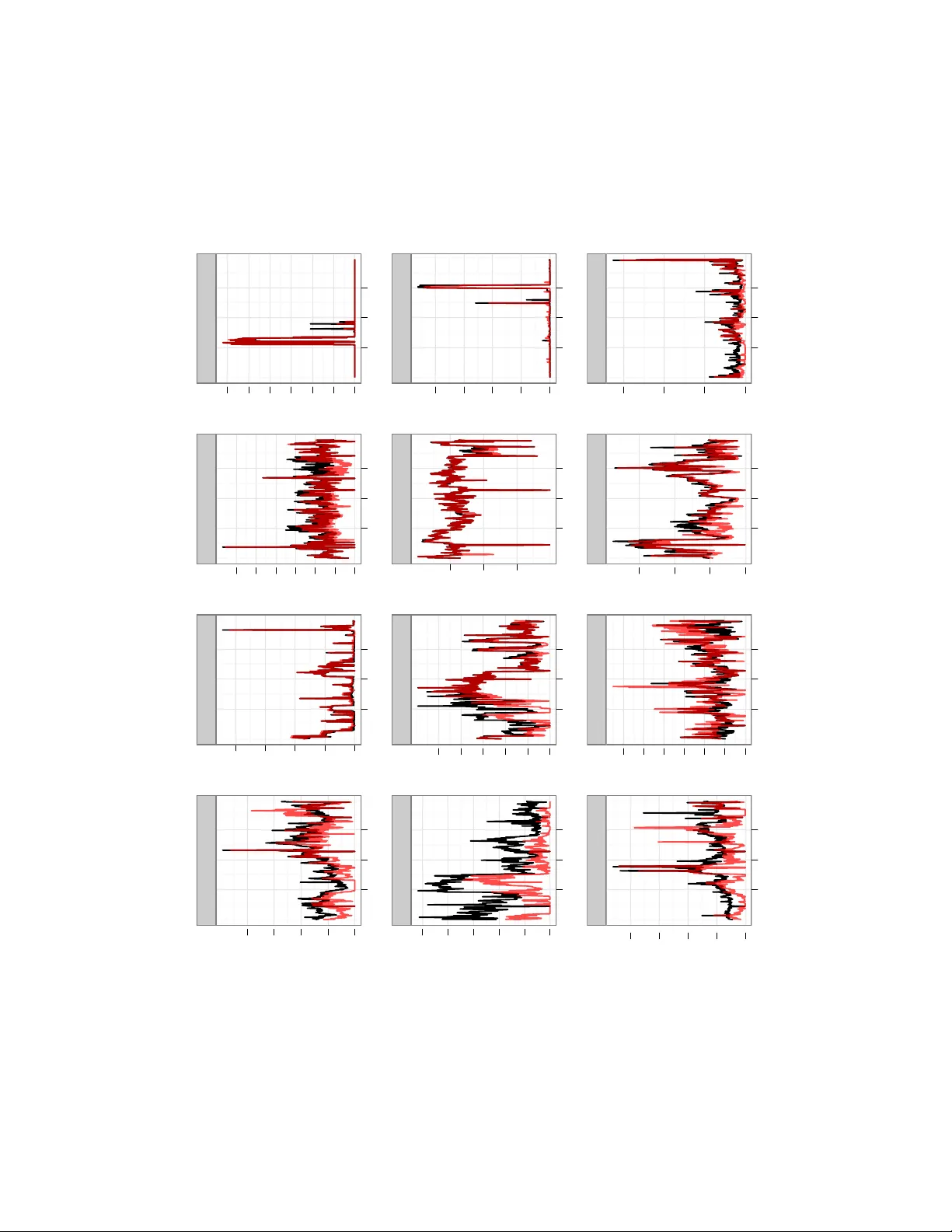
Decon volution of mixing time series on a graph Alexander W . Blocker Department of Statistics Harvard Uni versity Cambridge, MA 02138 Edoardo M. Airoldi Department of Statistics Harvard Uni versity Cambridge, MA 02138 Abstract In many applications we are interested in mak- ing inference on latent time series from indirect measurements, which are often lo w-dimensional projections resulting from mixing or aggregation. Positron emission tomography , super-resolution, and network traffic monitoring are some exam- ples. Inference in such settings requires solv- ing a sequence of ill-posed in verse problems, y t = A x t , where the projection mechanism pro- vides information on A . W e consider problems in which A specifies mixing on a graph of times se- ries that are bursty and sparse. W e develop a mul- tilev el state-space mo del for mixing times series and an ef ficient approach to inference. A simple model is used to calibrate regularization param- eters that lead to efficient inference in the mul- tilev el state-space model. W e apply this method to the problem of estimating point-to-point traf- fic flo ws on a network from aggregate measure- ments. Our solution outperforms existing meth- ods for this problem, and our two-stage approach suggests an efficient inference strate gy for multi- lev el models of multi variate time series. 1 INTR ODUCTION A perv asiv e challenge in the analysis of multiv ariate dy- namic data is the separation of individual time series from aggregate measurements, kno wn as decon volution. This flav or of inference problem arises in a number of appli- cations, including super-resolution imaging and positron emission tomography where we want to combine many 2D images in a 3D image consistent with 2D constraints ( Shepp and Kruskal , 1978 ; V ardi et al. , 1985 ); blind source separation where there are more s ources than observ ations (e.g., sound tracks) av ailable ( Lee et al. , 1999 ; Parra and Sajda , 2003 ; Liu and Chen , 1995 ); and inference on cells of a contingency table where two-w ay and multi-way mar - gins are giv en ( Bishop et al. , 1975 ; Dobra et al. , 2006 ). The core inference task underlying all of these problems is an ill-posed linear inv erse problem y = A x ( Hansen , 1998 ) where all the components of y , x are non-neg ativ e, and y has a lower dimensionality than x . W e explore an application of this decon volution problem known as dynamic network tomography: the problem of in- ferring origin-destination flo ws from aggregate traf fic on a communication netw ork ( V ardi , 1996 ). It is a classic prob- lem in the statistics and computer science literatures ( V an- derbei and Iannone , 1994 ; V ardi , 1996 ; T ebaldi and W est , 1998 ; Cao et al. , 2000 , 2001 ; Coates et al. , 2002 ; Medina et al. , 2002 ; Zhang et al. , 2003 ; Liang and Y u , 2003 ; Airoldi and F aloutsos , 2004 ; Lakhina et al. , 2004 ; Lawrence et al. , 2006 ; F ang et al. , 2007 ). Aggregate traffic flo ws measured ev ery fiv e minutes, y t , are modeled as a deterministic func- tion, A x t , of the routing matrix A and the individual origin- destination (OD) flo ws x t , ∀ t . The challenge is that the routing matrix A of size ( r × c ) is rank-deficient. In a net- work with n routers and switches, we typically measure r = O ( n ) aggreg ate traffic flows, and we need to infer c = O ( n 2 ) origin-destination flows at fiv e minute intervals. The inference task of interest is filtering, that is, inferring a distribution on x t giv en observations y 1: t up to time t (estimating P ( x t | y 1 , . . . , y t ) ). Predicting future OD flows x t + k is a separate, but related, task that relies on accurate filtering.          �    Figure 1: T raffic time-series on a network. The OD loads 1 → 2 and 1 → 3 are measured as aggreg ated load ∗ . Figure 1 illustrates this situation. Nodes in the network rep- resent routers and switches. Links between them represent cables connecting them. W e want to kno w the directed OD traffic flows from 1 to 2 and from 1 to 3. Howe ver , we can only measure aggregate directed traffic on the links, to which these OD traf fic flows both contrib ute. They cannot be distinguished without additional information. Here, we dev elop a multilev el state-space model that posits explicit probabilistic dynamics consisting of two layers. These layers provide a flexible, interpretable structure for inference and capture tw o vital properties of actual net- work traffic: spikes in traffic le vels and sparsity (an ab un- dance of time periods with small or zero traffic le vels). W e also dev elop a two-stage inference strategy for this model. W e first fit a simpler , identified Gaussian state- space model to our observed aggregate flows for calibra- tion. W e use these estimates to set regularization parame- ters for the probabilistic dynamics in the multile vel model, dev eloping a proposal for a sequential sample-importance- resample-mov e (SIRM) particle filter . The sampler is com- plemented by a ne w v ariant of the random directions sam- pler ( Smith , 1984 ), allowing for efficient inference in a complex dynamic setting. W e show that our two-stage in- ference scheme is more accurate than state-of-the-art meth- ods av ailable, scales to large networks (both in terms of speed of computation and in terms of efficiency of the se- quential SIRM sampler), and can be implemented in an on- line setting. The success of two-stage strategy relies only on the identifi- ability of the first-stage model, and can be applied to more general models of ill-posed linear in verse problems. The principle underlying our tw o-stage strate gy can be general- ized to other complex multilev el models. In this sense, our work is related to the recent body of work on “coarse-to-fine” learning techniques ( Geman , 2010 ; Bagnell , 2010 ; W eis and T askar , 2010 ), which in- clude a number of inference strategies for very lar ge data sets, for the most part, but also for complex models of medium size data sets, as in our problem setting. Coarse- to-fine learning strategies typically combine search strate- gies with inference strategies ( Langford , 2010 ). Our pro- posed strate gy is less focused on search algorithms; rather , it falls into the more statistical traditions of “principled cor- ner cutting” ( Meng , 2010 ) and data-dependent regulariza- tion ( Clogg et al. , 1991 ). 2 A MODEL OF MIXING TIME SERIES ON A GRAPH Giv en m observed traf fic counters over time, y it , the link loads, we want to make inference on n non-observable point-to-point traffic time series, x j t , origin-destination traffic flows. The routing scheme is parametrized by the routing matrix A , of size m × n . W e consider the case of a fixed routing scheme, in which the matrix A has binary en- tries. Entry a ij specifies whether traffic counter i includes the traffic volume on the origin destination j . W e dev elop a multilev el state-space model to explain the variability in the observed link loads. This data generat- ing process decouples the v ariability of the non-observ able origin destination time series, x 1: T , into a smooth linear process { λ t : t ≥ 1 } and an independent spike process { x t : t ≥ 1 } . The coefficient that drives the dynamics in the smooth linear proc ess introduces additional v ariability . V ariable dynamics are k ey for introducing calibrated regu- larization parameters in the two-stage estimation process. In detail, we posit that each OD flo w x i,t has its own time- varying intensity λ i,t . This underlying intensity e volves through time according to a multiplicativ e process log λ i,t = ρ log λ i,t − 1 + ε i,t where ε i,t ∼ N( θ 1 i,t , θ 2 i,t ) . This process leads to bursty traffic flows that are not sparse. Moreover , small differ - ences between low traffic flows receiv e quite different prob- abilities under this model. Thus, conditional on the under- lying intensity , we posit that the latent OD flows x i,t follow a truncated normal error model, x i,t | λ i,t , φ t ∼ T runcN (0 , ∞ )  λ i,t , λ τ i,t (exp( φ t ) − 1)  This error model induces sparsity while maintaining an- alytical tractability of the inference algorithms (see next Section) by decoupling sparsity control from the bursty dy- namic beha vior . The parameter τ provides some flexibility and it can be set with exploratory data analysis on the ob- served link loads. The mean-v ariance structure of the error model is analogous to that for a log-normal distribution; in particular , if log( z ) ∼ N( µ, σ 2 ) , E ( z ) = exp( µ + σ 2 / 2) and V ar ( Z ) = exp(2 µ + σ 2 ) · (exp( σ 2 ) − 1) . Thus, λ i,t is analogous to exp( µ + σ 2 / 2) , and φ t is analogous to σ 2 . The observed link flows are given by y t = A x t . W e com- plete our model by placing diffuse independent log-Normal priors on λ i, 0 . W e also place priors on φ t for stability , as- suming φ t ∼ Gamma( α, β t /α ) . The use of this multilevel structure provides a realistic model for the flows were are interested in, which are both bursty and sparse. The log-Normal layer provides bursty dynamics and replicates the intense spik es in traffic ob- served empirically , whereas the truncated Normal layer al- lows for very low traffic le vels with non-negligible proba- bility . By combining these two distributions, we obtain an ov erall distribution for our flo ws that allows for both ex- treme counts and sparsity , as can be seen in Fig. 2 . The proposed model is capable of generating data that qual- itativ ely resembles our observed flows. This includes the “spike” dynamics observed in the actual flows, as the ex- ample in Fig. 3 suggests.              �    Figure 2: Comparison of CDFs for λ i,t and x i,t Time T raffic 50000 100000 150000 Observed 5 10 15 20 Simulated 5 10 15 20 Figure 3: Actual & simulated OD flo ws 2.1 UNIMOD ALITY & POSTERIOR UPDA TES One important questi on about this model is how our pos- terior inferences will behav e under dynamic updates. If it tends to “grow” modes over time or exhibit other patho- logical behavior , our computation would be quite diffi- cult and our inferences would be less credible. Fortu- nately , this is not the case. In general, we have es- tablished that the quasiconcavity of a predictive distri- bution f ( x t | y t − 1 , . . . ) implies the quasiconca vity of the posterior f ( x t | y t , y t − 1 , . . . ) ; thus, the set of maxima for f ( x t | y t , y t − 1 , . . . ) will form a con vex set under the given condition. The proof of this is laid out in Theorem 1 : Theorem 1. Assume f ( x t ) is quasiconcave . Let y t = A x t . Then, f ( x t | y t ) will also be quasiconcave; in particular , it will have no separated modes (the set { z : f ( z | y t ) = max w f ( w | y t ) } is connected). Pr oof. f ( x t | y t ) ∝ I ( y t = A x t ) f ( x t ) , so f ( x t | y t ) has support on only a bounded r − c dimensional subspace of R c , which forms a closed, bounded, con vex polytope in the positi ve orthant. Denote this region B ( y t ) . Denote the mode of f ( x t ) as ˆ x t . W e no w consider two cases: 1. ˆ x t ∈ B ( y t ) . Then, the mode of f ( x t | y t ) is also ˆ x t . 2. ˆ x t / ∈ B ( y t ) . Then, we must be a bit more clever . Con- sider the level surfaces of f ( x t | y t ) , denoting C ( z ) = { u : f ( u | y t ) = z } . Define z ∗ = max B ( y t ) f ( x t | y t ) ; this is well-defined and attained as B ( y t ) is closed. Now , denoting C 0 ( z ) = { u : f ( u ) = z } , we ha ve C ( z ) = C 0 ( z )  B ( y t ) . As f ( x t ) is quasiconcave, its superle vel sets U 0 ( z ) = { u : f ( u ) ≥ z } are con- ve x. Thus, the superlev el sets of f ( x t | y t ) , denoted U ( z ) = U 0 ( z )  B ( y t ) analogously , are also con vex. So, we hav e that the set U ( z ∗ ) = C ( z ∗ ) is conv ex and non-empty . Therefore, we have established that set of modes for f ( x t | y t ) is con vex, hence connected. As we initialize our model with a unimodal (quasiconcave) log-Normal distribution and impose log-Normal dynam- ics on our underlying intensities λ t , the abov e theorem provides a useful limit on pathological behavior for our method. 3 INFERENCE W e no w outline the inference strategies and computational techniques de veloped to produce estimates from the pre vi- ously described model. W e use a sequential Monte Carlo algorithm (SIRM) to obtain estimates from our multilevel state-space model, yielding an efficient inference algo- rithm. The use of a random direction proposal on the feasible region for OD flows is a vital component of this method; without it, sampling these constrained v ariables would be difficult. Howe ver , ev en with such algorithmic re- finements, inference with our model remains difficult with- out further regularization. Therefore, we use a stable, iden- tifiable calibration model to estimate re gularization param- eters for our multile vel state-space model. This calibration step is described in detail below . 3.1 MODEL-B ASED REGULARIZA TION T o calibrate re gularization parameters for our generati ve model, we use a simpler model, assuming x t follows a Gaussian autoregressi ve process, in Eq 1 . This amounts to a standard Gaussian state-space formulation, detailed in Eq. 2 . The model we used to obtain the preliminary esti- mates for the OD flows is:  x t = F · x t − 1 + Q · 1 + e t y t = A · x t + � t (1) =         x t 1  =  F Q 0 I   x t − 1 1  +  e t 0  y t = [ A | 0 ]  x t 1  + � t =  ˜ x t = ˜ F · ˜ x t − 1 + ˜ e t y t = ˜ A · ˜ x t + � t . (2) W e estimate Q and Cov e t , fixing the remaining param- eters. F is fixed at ρ I for simplicity of estimation, with 0 . 1 a typical value for ρ . W e also fix Cov � t at σ 2 I , with 0 . 01 a typical value for σ 2 . W e assume Q to be a posi- tiv e, diagonal matrix, Q = diag ( λ t ) , and model Cov e t as Σ t = φ diag ( λ t ) τ , where the power is taken entry-wise. W e obtain inferences from this model via maximum like- lihood on overlapping windows of a fixed length. Imple- mentation details are discussed the next section. As the marginal lik elihood for this model depends only upon the means and cov ariances of our data, it will be iden- tifiable under conditions analogous to those gi ve in Cao et al. ( 2000 ). Maximum Likelihood Via Kalman Smoothing. Maxi- mum likelihood inference for our Gaussian SSM is feasi- ble with standard Kalman smoothing. T wo approaches to this maximization problem are possible: EM and direct nu- merical optimization. The EM approach, outlined for the unconstrained case by Ghahramani and Hinton ( 1996 ), re- quires Kalman smoothing for the E step and maximization of the expected log-likelihood for the M step. The former is straightforward and efficient to calculate using standard algorithms, but the latter requires expensi ve numerical op- timization in our case. Due to the constraints on Q and Co v e t and the dependence of our observ ations, there is no analytic form for the maximum of the expected log- likelihood under our model. Therefore, EM is less fa vor - able; linear con ver gence is a high price to pay when nu- merical optimization is required for either approach. W e instead use direct numerical optimization on the marginal likelihood obtained from the Kalman smoother , optimizing � ( Y | θ ) = −  t log | ˆ Σ t | − 1 2  t ( y t − ˆ y t ) � ˆ Σ − 1 t ( y t − ˆ y t ) where ˆ y t and ˆ Σ t are the estimated mean and covariance matrices from the Kalman smoother . W ith a fast (Fortran) implementation of the Kalman iterations, this approach yields fa vorable run-times and stable results. 3.2 SETTING REGULARIZA TION P ARAMETERS T o calibrate the regularization parameters for the parame- ters of the multilev el state-space model, we first run our es- timates from the Gaussian SSM at each time through IPFP (the iterati ve proportional fitting procedure) to ensure pos- itivity and validity with respect to our linear constraints. W e then run these estimates through IPFP , ensuring posi- tivity and feasibility for each estimate, and smooth these estimates using a running median with a small window (5 observations in our case), obtaining ˆ x t . These are used to set θ 1 i,t : θ 1 i,t = log ˆ x i,t − log ˆ x i,t − 1 The v ariability parameter θ 2 i,t is set using the estimated variance of each x i,t from our inference with the calibration model. Denoting this estimate as ˆ V i,t , we set θ 2 i,t as: θ 2 i,t = (1 − ρ 2 ) log (1 + ˆ V i,t / ˆ x 2 i,t ) Here, ρ is the (fixed) autocorrelation parameter in our model for the dynamics of log λ i,t . W e typically set ρ = 0 . 9 . W e fix ρ higher for this method than for our Gaussian SSM because more pooling of information across times is necessary . While the Gaussian SSM is identifiable with a sufficiently wide windo w , our multilevel state-space model relies more strongly on dependence between flows at sim- ilar times to obtain information on the underlying param- eters and OD flows. Therefore, a larger value amount of autocorrelation is required to obtain stable estimation. Fur- thermore, a high value for ρ is a practically plausible as- sumption, as OD flows tend to be highly autocorrelated in communication networks ( Cao et al. , 2002 ). 3.3 MUL TILEVEL ST A TE-SP A CE INFERENCE: SIRM FIL TER Inference in the multilevel state-space model is performed with a sample-resample-mov e algorithm, akin to Gilks and Berzuini ( 2001 ); its structure is outlined in Algorithm 1 . Sample-Importance-Resample-Move algorithm for t ← t to T do Sample step: for j ← 1 to m do Draw a proposal log λ ( j ) ∗ i,t ∼ N( θ 1 i,t + log λ ( j ) i,t − 1 , θ 1 i,t ) Draw φ ( j ) t ∼ Gamma( α, ˆ φ t /α ) Draw x ( j ) ∗ t from a truncated Normal distribution with mean µ ∗ = θ 1 t + ρ/m  m j =1 λ ( j ) t − 1 and cov ariance matrix Σ ∗ = (exp( ˆ φ t ) − 1)diag  µ ∗ 2  on the feasible region giv en by x ( j ) ∗ t ≥ 0 , y t = Ax ( j ) ∗ t using Algorithm 2 Resample our particles ( λ ( j ) ∗ t , φ ( j ) ∗ t , x ( j ) ∗ t ) with probabilities proportional to our weights w ( j ) t Mov e each of our resampled particles ( λ ( j ) t , φ ( j ) t , x ( j ) t ) using a MCMC algorithm (Metropolis-Hastings within Gibbs, with proposal on x t giv en by Algorithm 2 ) retur n ( λ ( j ) t , φ ( j ) t , x ( j ) t ) for j ← 1 to m , t ← 1 to T Algorithm 1 : SIRM algorithm for inf erence with multi- lev el state-space model W e use the approach o f Smith ( 1984 ), known as the “ran- dom directions algorithm” (RD A), to sample from dis- tributions on constrained re gions in our algorithm. This method constructs a random-walk proposal on con vex re- gions (such as our feasible re gions for x t ) by first drawing a v ector d uniformly on the unit sphere. W e then calculate the intersections of a line along this vector with the sur- face of the bounding region and sampling uniformly along the feasible se gment of this line. This feasible segment can be calculated easily using the decomposition of A giv en by T ebaldi and W est ( 1998 ). They decompose A as [ A 1 A 2 ] by permuting the columns of A (and the corresponding com- ponents of x t , where A 1 ( r × r ) is of full rank. Then, splitting the permuted vector x t = [ x � 1 ,t x � 2 ,t ] , we obtain x 1 ,t = A − 1 1 ( y t − A 2 x 2 ,t ) . This formulation can be used to construct an efficient random directions algorithm to pro- pose valid values of x t ; we have included pseudocode for this algorithm in Algorithm 2 . Random Directions Algorithm Initialization begin Decompose A into [ A 1 A 2 ] , A 1 ( r × r ) full-rank as in T ebaldi and W est ( 1998 ) Store B := A − 1 1 ; C := A − 1 1 A 2 end Metropolis step given x t begin Draw z ∼ N (0 , I ) , z ∈ R c − r Set d := z / � z � Calculate w : = C · d Set h 1 := max { min k : w k > 0 ( x 1 ,t ) k /w k , 0 } Set h 2 := max { min k : d k < 0 − ( x 2 ,t ) k /d k , 0 } Set h := min { h 1 , h 2 } Set l 1 := max { max k : w k < 0 ( x 1 ,t ) k /w k , 0 } Set l 2 := max { max k : d k > 0 − ( x 2 ,t ) k /d k , 0 } Set l := max { l 1 , l 2 } Draw u ∼ Unif ( l , h ) Set x ∗ 2 ,t := x 2 ,t + u · d ; x ∗ 1 ,t = x 1 ,t − u · w ; x ∗ t = ( x ∗ 1 ,t , x ∗ 2 ,t ) Set x t := x ∗ t with probability min { f ( x ∗ t ) /f ( x t ) , 1 } end retur n x t Algorithm 2 : RDA algorithm for sampling from f ( x t ) , truncated to the feasible region giv en by A · x t = y t All draws from this proposal have positiv e posterior density (as they are feasible). This property allows our sampling methods to move away from problematic boundary regions of the gi ven feasible polytope; methods that use, for ex- ample, Gaussian random-walk proposal rules can perform quite poorly in these situations, requiring an extremely large number of draws to obtain feasible proposals. For example, with x t ∈ R 16 , it can sometimes require 10 9 or more draws to obtain a v alid particle using the conditional posterior from t − 1 as a proposal with the datasets tested in Section 5 . 4 SIMULA TION STUD Y T o ev aluate our inference algorithm, we simulated OD flows from our multilev el state-space model under 3 net- work topographies: a 3-node bidirectional chain, a 3-node star topography , and a 4-node start topography , correspond- ing to 2, 4, and 9-dimen sional latent spaces for our infer- ence on x t . For each of these cases, we produced 30 repli- cates consisting of 300 time-points. W e then calculated the link flows for each replicate and ran our inference algo- rithm. In addition to the two-stage approach outlined pre- viously , we also performed filtering using our multile vel state-space model with a na ¨ ıve random-walk regularization on the OD flo ws; that is, we set θ 1 i,t = 0 ∀ ( i, t ) and θ 2 i,t = log(5) / 2 . This allows us to directly ev aluate the effect of our regularization strate gy and plausibility of our model. The primary quantity of interest in our simulations are the relativ e mean L 2 and L 1 errors in estimated OD flows for for the na ¨ ıve regularization compared to our two-stage method. The distributions of these relative errors is sum- marized in Figure 4 . Dimensionality of problem Relative L 2 error 0.5 1.0 1.5 2.0 2.5 � � � � � � � � 2 4 9 Dim 2 4 9 Figure 4: Relativ e L 2 error for na ¨ ıve vs. two-stage method against dimensionality W e find that our two-stage method outperforms one us- ing a na ¨ ıve re gularization. The decreasing variation in our relativ e errors suggests that the consistency of this out- performance increases with dimensionality . Specifically , we hav e a mean relative error of 1 . 09 ± 0 . 49 in 2 di- mensions, increasing to 1 . 57 ± 0 . 45 in 4 dimensions and 1 . 40 ± 0 . 26 in 9 dimensions. Our experience with these simulations also highlighted the computational benefits of our two-stage strategy . During particle filtering iterations with the na ¨ ıve regularization, the effecti ve number of par - ticles rarely climbed abov e 2, whereas we typically ob- tained 10 − 50 with the two-stage approach (with an equiv- alent number of particles). W ith real data, we expect ad- ditional benefits from our two-stage approach; in particu- lar , we would e xpect it to ha ve greater robustness to model misspecification. W e are using information from a simpler model to rein-in potential issues with more the more deli- cate hierarchical model, which should stabilize inferences from the latter and limit problems of non-identifiability . These expectations are borne out in Section 5 . 5 EMPIRICAL RESUL TS W e present two datasets from the field of network tomog- raphy , one spanning 4 nodes (16 OD flows) and the other spanning 12 nodes (144 OD flo ws), upon which we ev alu- ate our two-stage decon volution method. W e compare the performance of our approach to that of several previously presented in the literature for this problem, focusing on ac- curacy , computational stability , and scalability . 5.1 D A T ASETS Our first dataset is that of Cao et al. ( 2000 ). W e use their “Router1” network, consisting of 4 nodes in a star topogra- phy (yielding 8 observed link flows) with 16 OD flows. The data consists of link flows observed e very 5 minutes over 1 day on a Bell Labs corporate network. This yields 287 times, providing a rich dataset for in vestigation of the use of dynamic information in network tomography . The small size of this network allows us to focus on the fundamentals of the problem without focusing on issues of scalability . For further in vestigation, we constructed a dataset from 2 days of observed OD flows on the CMU network. The routing table for this network is sensitive (due to network security issues), so we combined actual OD flows in a syn- thetic network topography . This network topology consists of 12 nodes. These are connected in a star topography to two routers (one with 4 of the nodes, the other with the re- maining 8); the routers are linked via a single connection. This configuration yields 26 observed link flows and 144 OD flo ws, observ ed ov er 473 times (5 minute intervals). This larger dataset allo ws for the comparison of network tomography techniques in a richer, more realistic setting. In combination with the “Router1” data, it also allows us to explore the effect of dimensionality on performance and computational efficienc y .                      Figure 5: Bell Labs and CMU network structures. W e do not apply an y seasonal adjustment or other more complex dynamic models to these datasets. W e would rec- ommend such an extension for data spanning longer pe- riods; indeed, even for data spanning only two days, us- age patterns by time-of-day can be significant. Ho we ver , we endeavour to compare our decon volution algorithms on equal footing – our focus is dynamic decon volution. Thus, all methods are implemented with only local dynamics (no seasonal adjustment). 5.2 COMPETING METHODS W e tested the locally IID and smoothed methods of Cao et al. ( 2000 ), the Bayesian MCMC approach of T ebaldi and W est ( 1998 ), our multilev el state-space model with na ¨ ıve regularization (as in Section 4 ), and our two-stage approach (Gaussian SSM follo wed by multilev el state-space model). All approaches were implemented in R with extensions in C for particular bottlenecks (e.g. IPFP). For the methods of Cao et al. ( 2000 ) and our Gaussian SSM, which use win- dowed estimates, we used a window width of 23. For the approach of T ebaldi and W est ( 1998 ), we tested both the original implementation and our o wn modifica- tion in which (following the authors’ original notation) λ j and X j are sampled with a joint Metropolis-Hastings step. The proposal distribution for this step is constructed by first proposing uniformly along the range of feasible val- ues for X j giv en all other values, then dra wing λ j from its conditional posterior given the proposed X j . This greatly improv es the ef ficiency of inference for their model, lead- ing to improved conv ergence (we observed multiv ariate Gelman-Rubin diagnostics reduced by approximately an order of magnitude) and better predictions. These improve- ments allo w us to compare our model to theirs on a more lev el playing field, focusing on the underlying model rather than computational issues. 5.3 PERFORMANCE COMP ARISON W e summarize performance of the previously mentioned methods on both datasets in T able 1 . Each row corresponds to a method, and the columns provide average L 1 and L 2 errors for the estimates of OD flows in each dataset with corresponding standard errors. For the Bell Labs dataset, we provide errors in kilobytes; for the CMU data, we pro- vide errors in megabytes. W e also provide Figures S1 - S5 in our supplemental material as a visualization of our re- sults on the Bell Labs dataset. W e compare performance in accuracy , computational stability , and scalability . Accuracy . W e obtain fa vorable performance for our two- stage approach (corresponding the final row of T able 1 ) for both datasets. Mean L 1 and L 2 errors for this method are within 1 SE of the minimum for the Bell Labs data. Both of our methods reduce av erage L 1 and L 2 errors by 60 - 80% T able 1: Performance Comparison (Bell Labs results in Kb, CMU results in Mb. * Denotes our own impro vement on the original algorithm by T ebaldi & W est) BELL LABS CMU Method L 2 Error SE L 1 Error SE L 2 Error SE L 1 Error SE Locally IID model 104.59 5.54 160.24 6.53 592.49 9.91 1169.15 17.11 Smoothed locally IID 104.25 5.52 157.87 6.48 — — — — T ebaldi & W est (uniform prior) 76.60 4.91 173.94 7.49 — — — — T ebaldi & W est (joint proposal)* 49.43 2.58 147.66 6.18 167.94 4.42 712.37 14.68 Dynamic multilev el model (na ¨ ıve) 63.29 3.35 178.43 8.09 311.21 6.25 1109.68 19.58 Calibration model (stage 1) 19.35 0.72 57.66 2.06 110.47 6.19 389.14 16.72 Dynamic multilev el model (stage 2) 19.93 0.87 58.20 2.39 93.42 5.20 334.74 13.64 compared to the other approaches presented, representing a major g ain in predictiv e accuracy . For the CMU data, we obtain a reduction of 53% in av erage L 2 error and 44% in av erage L 1 error from the algorithm of T ebaldi and W est ( 1998 ) to our multilevel state-space model; we observe 14 - 15% reductions in average L 1 and L 2 errors from our Gaussian SSM to the multilevel state-space models. Fur- thermore, we observe large gains in filtering performance for both datasets compared to inference using na ¨ ıve regu- larization with our multilevel state-space model. Overall, our approach outperforms existing methods in accuracy , with greater gains from the Gaussian SSM to the multilevel state-space model in our higher-dimensional setting. The three last methods in T able 1 each contain a mix of three attributes: explicit dynamics, skewness, and regu- larization to improv e identifiability . Our multilev el state- space model with na ¨ ıve regularization incorporates the for- mer two, but its performance suffers from problems with identifiability . Our calibration model is identifiable and incorporates explicit dynamics, but does not account for ske wness. It performs well on the Bell Labs dataset, where that distrib utions of OD flows are relatively symmetric, but suf fers on the extremely skewed CMU dataset. Our two-stage procedure using the multilev el state-space model ov ercomes identifiability issues and accounts for skewness, attaining comparable performance with the Bell Labs net- work and outperforming considerably on the CMU network as a result. Computational stability . The methods tested varied in computational stability . Those of Cao et al. ( 2000 ) re- mained stable across both datasets, b ut the original method of T ebaldi and W est ( 1998 ) encountered issues. On the Bell Labs data, it required a very large number of iterations to obtain con vergence (as indicated by the Gelman-Rubin diagnostic); 150,000 iterations per time were used to pro- vide the given estimates, 50,000 of which were discarded as burn-in. This method failed completely on several times in the CMU data, becoming trapped in a corner of the feasible region. Our revised version of their algorithm performed much better , requiring far fe wer iterations for con ver gence (50,000 was suf ficient for all examined cases, but 150,000 were used for the results presented for comparability). Our calibration model proved computationally stable across both datasets. T he direct use of marginal likelihood, for maximum likelihood estimation, proved effecti ve even in a high-dimensional setting. The multilev el state-space model was also stable in both settings with the giv en struc- ture; howe ver , it was sensitive to some of the points men- tioned in Section 3 . Major problems arose in experiments using the posterior on x t from the pre vious time as a pro- posal (as is common in applications of particle filtering); sev eral times in the Bell Labs data required ov er 10 mil- lion proposals to obtain a single feasible particle. Addi- tional care was needed with the “move” step due to simi- lar issues. Furthermore, the use of a na ¨ ıve, random-walk regularization caused some computational difficulties, as the particles often became extremely diffuse in the feasi- ble region. Overall, we found inference with the multi- lev el state-space model computationally stable so long as sampling methods for highly constrained variables ( x t in particular) explicitly respected said constraints, proposing only v alid v alues. Our random directions algorithm (Algo- rithm 2 ) handles this task well. Scalability . All methods ev aluated fared well in scala- bility , including our computationally-intensiv e, simulation- based inference using the multilev el state-space model. W e focus first on the run-times for the CMU dataset. For each time, the methods of Cao et al. ( 2000 ) required approx- imately 225 seconds to obtain maximum likelihood esti- mates with a 23 observation window . Our modification of T ebaldi and W est ( 1998 ) required approximately 1500 sec- onds to obtain 150,000 samples for a single time; the orig- inal (where it ran) required 2250 seconds on average. In contrast, our simulation-based filtering method for the mul- tilev el state-space model required 270 seconds per time on av erage. For the Bell Labs dataset, our filtering method required approximately 8 seconds per time, whereas our modification of T ebaldi and W est ( 1998 ) required 150 sec- onds per time and their original algorithm required approx- imately the same. These results are encouraging: the fil- tering component of our method, which would be the part used in online applications, is reasonably efficient (ev en written in R) and could run in faster than real-time with 144 OD flo ws at 5 minute sampling intervals. Given more effi- cient implementation and parallelization (which is feasible for all sampling steps), this approach can scale to prob- lems of the scale typically found in the real-world. This is especially true gi ven the sparsity of man y such flo ws on networks; the prev alence of zero aggregate (link) flows in real-world data reduces the effectiv e size of the deconv olu- tion problem. 6 REMARKS W e have addressed the decon volution of time-series on a graph, with an application to dynamic network tomogra- phy . For this problem, we dev elop a novel statistical ma- chine learning approach to inference by combining a nov el two-stage strategy with a new multilevel state-space model that posits non-Gaussian marginals and nonlinear proba- bilistic dynamics. Our results and analyses substantiate sev eral claims and suggest points for further discussion. T o demonstrate our method, we analyzed two networks, at Bell Labs and CMU, which span substantial range of di- mensionality , with different inference methods. The results demonstrate a clear improv ement of the proposed method- ology over previously published methods in reconstructing OD flows in two network tomography settings. Compari- son between Bell Labs and CMU results suggests that this gain increases with the dimensionality of the problem. 6.1 MODELING AND COMPUT A TIONAL ISSUES Our model e xplicitly captures two critical feature of our time series — namely , skewness and temporal dependence. A large portion of the substantial improvements in accu- racy ov er existing methods can be attrib uted to these mod- eling improvements. The gains in computational efficienc y account for only part of the improvements in accuracy — see below . Pre vious approaches have included skewness ( T ebaldi and W est , 1998 ), but nev er explicit temporal de- pendence of the OD flows. The inter-temporal smoothing algorithm of Cao et al. ( 2000 ) includes elements of tem- poral dependence; howe ver , the model assumed temporally independent OD flo ws and the dependence is on the width of the windo ws of observations that contribute to inference of the OD flows for each time point. In summary , previ- ous work has not accounted for the range of properties ad- dressed here. The performance gains from such modeling are clear in the two datasets tested; in particular , the gains from the model of T ebaldi and W est ( 1998 ) to the Gaus- sian SSM and the final multilevel state-space model for the CMU data reinforce the benefits of using a realistic model in this problem. Fundamentally , we estimate the OD flows by projecting our observations onto the latent space the flows inhabit; that is, we want to compute E [ x t | y t ] under a giv en probabilistic structure. The relative v ariability of OD flows over time plays a large role in inference, as their is typically a strong relationship between the mean and v ariance of OD flows. Because of this, simple methods that do not model variabil- ity explicitly and realistically , including Moore-Penrose generalized in verse ( Harville , 2008 ), independent compo - nent analysis ( Hyv ¨ arinen et al. , 2003 ), and iterativ e propor- tional fitting procedure ( Fienberg , 1970 ) are of limited use in this conte xt. Our approach, in contrast, models this v ari- ability with a probabilistic structure, improving inferences by using this additional information. Our inference method is computationally efficient and scales to large networks than ha ve been previously ad- dressed using probabilistic models. The problem is funda- mentally O ( c ) for each time observed, so we cannot hope to do better than quadratic scaling in the number of nodes in our network (excepting cases where link loads are 0). De- spite the sophistication of our multilev el state-space model, our sequential Monte Carlo technique allows for inference in better than real-time for a network with 144 OD flows. As this is the component that would be used in an online application, we ha ve demonstrated a scalable technique for inference with a model of greater complexity and realism than has been previously found in the literature. These gains in computational efficienc y also reduce nu- merical instability and are ultimately responsible for ad- ditional gains in accuracy . Computational issues can be appreciated by considering the amount of ef fort we needed to place in maintaining Cov e t positiv e-definite in the EM algorithm of Cao et al. ( 2000 ), especially when the traffic approaches zero. W e can see some artifacts in the corre- sponding OD estimates in Figure S1 (green lines) due to this issue in the lo w traffic OD flows, e.g. “orig local, dest local”. W e further quantified the ef fects of computational efficienc y on inference in the original methods by T ebaldi and W est ( 1998 ) in T able 1 by comparing the uniform prior and component-wise proposal to the joint proposal we de- veloped. In addition to the gains in speed and conv ergence discussed in Section 5.3 , we observe a large reduction in av erage error from the component-wise to joint proposal ( 35% in L 2 error , 15% in L 1 ) with no change in priors or the underlying model. The use of the random directions algorithm (of Smith ( 1984 )) in our sequential Monte Carlo method is vital. W ithout such an algorithm to sample directly on the fea- sible region for each set of OD flows, we would be forced to use a nai ve proposal distribution. In our testing, such distributions prov ed e xtremely problematic (as discussed in Section 3 ), especially in higher dimensional settings. In such cases, sampling strategies that fully utilize the av ail- able constraint information are necessary to obtain high ac- curacy and efficienc y . This is particularly salient compar- ing the results presented here to our previous work ( Airoldi and Faloutsos , 2004 ); the method presented in that work suffered from computational instabilities, requiring restarts of its filtering algorithm at particular time points. It was also hampered by inefficient sampling on the feasible re- gion and distributional assumptions (the log-Normal was used as the distribution of x t | λ t ) that induced issues in modeling OD flows near zero. Recently proposed sam- pling strate gies ( Airoldi and Haas , 2011 ) will likely im- prov e computational performance and the estimates. Last, multi-modality in the marginal posterior on each OD flow x it appears low to non-existent in our in vestigations. Howe ver T ebaldi and W est ( 1998 ) and Airoldi and Falout- sos ( 2004 ) have observed a substantial amount of multi- modality in their results. Our results suggest that the theo- retical amount of multi-modality in these problems is low for the case of real-valued OD flo ws and models assum- ing independent OD flows. The amount of multi-modality observed in previous work appears to originate primarily from the inefficiency of the samplers and, to a lesser ex- tent, the assumption of discrete-valued OD flo ws. This further reinforces the importance of ef ficient computation for inference in complex, weakly identified settings; even a simple model can f alter on poor computation, and comple x models require great computational care to obtain reliable inferences. 6.2 A NO VEL TWO-ST A TE STRA TEGY FOR INFERENCE IN D YNAMIC MUL TILEVEL MODELS As previously argued by T ebaldi and W est ( 1998 ) in the static setting, informativ e priors are essential to identify a unique posterior mode that approximates the true config- uration of OD flows well. This is remains true in the dy- namic setting, despite the additional information that tem- poral dependence makes rele vant for the inference of each OD flow . The technical choices at issue are: (i) where to find such information that it is not obvious in the data; (ii) what parameters are most con venient to put priors on; and (iii) ho w do we translate the additional information into prior information for the chosen parameters. W e use a simple nearly identifiable model, which is not as realistic as our multilev el state-space model, to find rough estimates of the OD flows (in our first-stage). These esti- mates provide some information about where the OD flows are in the space of feasible solutions, enabling us to iden- tify high-probability subsets of the feasible region at each time before embarking on computationally-intensiv e sim- ulations. This effect is larger in higher dimensions, as the proportion of the feasible region’ s volume with high pos- terior density decreases rapidly with dimensionality (the classical curse of dimensionality). Practically , informati ve priors increase the ef ficiency of the particle filter by fo- cusing its sampling on promising regions of the parameter space, av oiding wasted computation and improving infer- ences. In order to pass the first-stage information to the (non- Gaussian) multilevel state-space model, we mo ved aw ay from a standard linear state-space formulation with additive error to a non-linear formulation with stochastic dynamics, which ef fectiv ely provides a multiplicati ve error (second- stage). The stochastic dynamics assumed for λ t provide our parameters of choice for the incorporation of this in- formation; adding this layer of variability to our model al- lows our regularization to guide inferences without placing too tight a constraint on the inferred OD flows. In Sec- tion 3 we described the problem we solve to translate the first-stage estimates into regularization for the parameters of the second-stage model. W e traded off the need to pass as much of this information as possible from the first- to second-stage with the known inaccuracy of the first-stage. Our two-stage procedure suggests a more general strategy for inference in complex hierarchical models with mild identifiability issues. Using simpler models to guide com- putation with more sophisticated, realistic models and (if necessary) provide regularization can provide large gains in performance. W e have demonstrated the utility of this prin- cipled approach to “cutting corners”. This approach has allowed us to use a sophisticated generativ e model for in- ference, le veraging the po wer of multile vel analysis, while maintaining efficienc y for real-time applications. W e look forward to inv estigating its utility in other settings, includ- ing predicting flows of communications within social net- works from aggregate measurements and inferring biologi- cal fluxes from e xperimental data. References E. M. Airoldi and C. Faloutsos. Recovering latent time- series from their observed sums: network tomography with particle filters. In Pr oceedings of the ACM SIGKDD International Confer ence on Knowledge Discovery and Data Mining , volume 10, pages 30–39, 2004. E. M. Airoldi and B. Haas. Polytope samplers for inference in ill-posed in verse problems. In International Confer- ence on Artificial Intelligence and Statistics , volume 15, 2011. D. Bagnell. Learning hierarchical inference machines. T alk at NIPS 2010 workshop on coarse-to-fine learning and inference, December 2010. Y . Bishop, S. E. Fienberg, and P . Holland. Discrete mul- tivariate analysis: theory and practice . The MIT press, 1975. J. Cao, D. Davis, S. V an Der V iel, and B. Y u. T ime-varying network tomography: router link data. Journal of the American Statistical Association , 95:1063–75, 2000. J. Cao, D. Davis, S. V an Der V iel, B. Y u, and Z. Zu. A scalable method for estimating network traffic matrices from link counts. T echnical report, Bell Labs, 2001. J. Cao, W . S. Cleveland, D. Lin, and D. X. Sun. The effect of statistical multiplexing on the long range dependence of internet packet traffic. T echnical report, Bell Labs, 2002. C. C. Clogg et al. Multiple imputation of industry and occupation codes in census public-use samples using Bayesian logistic regression. Journal of the American Statistical Association , 86(413):68–78, 1991. A. Coates, A.O. Hero III, R. Nowak, and Bin Y u. Internet tomography . Signal Pr ocessing Magazine, IEEE , 19(3): 47 –65, may 2002. A. Dobra, C. T ebaldi, and M. W est. Data augmentation in multi-way contingency tables with fixed marginal to- tals. Journal of Statistical Planning and Inference , 136 (2):355–372, 2006. J. Fang, Y . V ardi, and C.-H. Zhang. An iterative tomo- gravity algorithm for the estimation of network traffic. In R. Liu, W . Strawderman, and C.-H. Zhang, editors, Complex Datasets and In verse Pr oblems: T omography , Networks and Be yond , volume 54 of Lectur e Notes– Monograph Series . IMS, 2007. S. E. Fienberg. An iterativ e procedure for estimation in contingency tables. The Annals of Mathematical Statis- tics , 41(3):907–917, 1970. D. Geman. Cats and dogs. T alk at NIPS 2010 workshop on coarse-to-fine learning and inference, December 2010. Z. Ghahramani and G. E. Hinton. Parameter estimation for linear dynamical systems. T echnical Report CRG- TR-96-2, Department of Computer Science, Univ ersity of T oronto, 1996. W .R. Gilks and C. Berzuini. Follo wing a Moving T arget- Monte Carlo Inference for Dynamic Bayesian Models. Journal of the Royal Statistical Society . Series B, Statis- tical Methodology , 63(1):127–146, 2001. P . C. Hansen. Rank-deficient and discr ete ill-posed prob- lems: Numerical aspects of linear in version . SIAM, 1998. D. A. Harville. Matrix Algebra F r om a Statistician’s P er- spective . Springer , 2008. A. Hyv ¨ arinen, J. Karhunen, and E. Oja. Independent Com- ponent Analysis . John W iley & Sons, 2003. A. Lakhina et al. Structural analysis of network traf fic flows. SIGMETRICS P erform. Eval. Rev . , 32:61–72, June 2003. J. Langford. NIPS 2010. Blog post no. 1614, December 2010. (http://hunch.net/?p=1614) E. Lawrence, G. Michailidis, V . Nair , and B. Xi. Network tomography: A re view and recent developments,. In J. Fan and H. L. Koul, editors, F r ontiers in Statistics . Imperial College Press, 2006. T .-W . Lee, M. S. Lewicki, M. Girolami, and T . J. Se- jnowski. Blind source separation of more sources than mixtures using o vercomplete representations. IEEE Sig- nal Pr ocessing Letters , 6(4):87–90, 1999. G. Liang and B. Y u. Pseudo-likelihood estimations in net- work tomography . In Pr oceedings of IEEE INFOCOM , 2003. J. S. Liu and R. Chen. Blind Decon volution via Sequential Imputations Journal of the American Statistical Associ- ation , 90(430):567–576, 1995. A. Medina, N. T aft, K. Salamatian, S. Bhattacharyya, and C. Diot. T raffic matrix estimation: existing techniques and ne w directions. SIGCOMM Computer Communica- tion Revie w , 32(4):161–174, 2002. X. L. Meng. Machine learning with human intelligence: Principled corner cutting ( pc 2 ) . Plenary In vited T alk, Annual Conference on Neural Information Processing Systems (NIPS), December 2010. L. Parra and P . Sajda. Blind source separation via gener- alized eigen value decomposition. Journal of Machine Learning Resaer ch , 4:1261–1269, 2003. L. A. Shepp and J. B. Kruskal. Computerized tomogra- phy: The new medical x-ray technology . The American Mathematical Monthly , 85(6):420–439, 1978. R. L. Smith. Efficient monte carlo procedures for gener- ating points uniformly distributed over bounded regions. Operations Researc h , 32(6):pp. 1296–1308, 1984. C. T ebaldi and M. W est. Bayesian inference on network traffic using link count data. Journal of the American Statistical Association , 93(442):557–573, 1998. R. J. V anderbei and J. Iannone. An em approach to od ma- trix estimation. T echnical Report SOR 94-04, Princeton Univ ersity , 1994. Y . V ardi. Network tomography: estimating source- destination traf fic intensities from link data. Journal of the American Statistical Association , 91:365– 377, 1996. Y . V ardi, L. A. Shepp, and L. Kaufman. A statistical model for positron emission tomography . Journal of the Amer- ican Statistical Association , 80(389):8–20, 1985. D. W eis and B. T askar . Structured prediction cascades. In Pr oceedings of the 13th International Confer ence on Ar- tificial Intelligence and Statistics (AIST ATS) , volume 6. Journal of Machine Learning Research W&CP , 2010. Y . Zhang, M. Roughan, C. Lund, and D. Donoho. An information-theoretic approach to traf fic matrix estima- tion. In Pr oceedings of SIGCOMM , 2003. A APPENDIX – SUPPLEMENT ARY MA TERIAL In this appendix, we show the actual vs. fitted OD flows for the methods presented pre viously . W e plot all OD flows for the Bell Labs data and the 12 most variable OD flows for CMU. Ground truth is always in black, with estimated values in color . Figures S1 through S5 cov er the Bell Labs data, and Figures S6 through S10 cover the CMU data. Time (hours) T raffic (kilob ytes/sec) 0 100 200 300 400 0 200 400 600 800 50 100 150 200 250 100 200 300 400 500 600 orig cor p 5 10 15 20 orig fddi 5 10 15 20 orig local 5 10 15 20 orig switch 5 10 15 20 dest cor p dest fddi dest local dest switch Figure S1: Fitted values vs. ground truth for Bell Labs data. Ground truth in black; Locally IID model in green. Time (hours) T raffic (kilob ytes/sec) 0 100 200 300 400 0 200 400 600 800 50 100 150 200 250 100 200 300 400 500 600 orig cor p 5 10 15 20 orig fddi 5 10 15 20 orig local 5 10 15 20 orig switch 5 10 15 20 dest cor p dest fddi dest local dest switch Figure S2: Fitted values vs. ground truth for Bell Labs data. Ground truth in black; T ebaldi & W est (joint proposal) in blue. Time (hours) T raffic (kilob ytes/sec) 0 100 200 300 400 0 200 400 600 800 0 50 100 150 200 250 0 100 200 300 400 500 600 orig cor p 5 10 15 20 orig fddi 5 10 15 20 orig local 5 10 15 20 orig switch 5 10 15 20 dest cor p dest fddi dest local dest switch Figure S3: Fitted values vs. ground truth for Bell Labs data. Ground truth in black; Calibration model (stage 1) in purple. Time (hours) T raffic (kilob ytes/sec) 0 100 200 300 400 0 200 400 600 800 50 100 150 200 250 300 100 200 300 400 500 600 orig cor p 5 10 15 20 orig fddi 5 10 15 20 orig local 5 10 15 20 orig switch 5 10 15 20 dest cor p dest fddi dest local dest switch Figure S4: Fitted v alues vs. ground truth for Bell Labs data. Ground truth in black; Dynamic multile vel model (stage 2) in red. Time (hours) T raffic (kilob ytes/sec) 0 100 200 300 400 0 200 400 600 800 50 100 150 200 250 100 200 300 400 500 600 orig cor p 5 10 15 20 orig fddi 5 10 15 20 orig local 5 10 15 20 orig switch 5 10 15 20 dest cor p dest fddi dest local dest switch Figure S5: Fitted values vs. ground truth for Bell Labs data. Ground truth in black; Na ¨ ıve prior in orange. Time (hours) T raffic (megab ytes) 50 100 150 200 20 40 60 80 100 20 40 60 80 od1 10 20 30 od41 10 20 30 od124 10 20 30 500 1000 1500 2000 20 40 60 80 100 20 40 60 80 od5 10 20 30 od78 10 20 30 od125 10 20 30 0 20 40 60 80 100 120 500 1000 1500 0 50 100 150 od22 10 20 30 od85 10 20 30 od127 10 20 30 0 100 200 300 400 500 600 0 100 200 300 400 50 100 150 od30 10 20 30 od112 10 20 30 od143 10 20 30 Figure S6: Fitted values vs. ground truth for CMU data. Ground truth in black; Locally IID model in green. Time (hours) T raffic (megab ytes) 0 50 100 150 200 0 20 40 60 80 100 0 20 40 60 80 od1 10 20 30 od41 10 20 30 od124 10 20 30 0 500 1000 1500 2000 0 20 40 60 80 100 0 20 40 60 80 100 od5 10 20 30 od78 10 20 30 od125 10 20 30 0 20 40 60 80 100 120 0 500 1000 1500 0 50 100 150 od22 10 20 30 od85 10 20 30 od127 10 20 30 0 100 200 300 400 500 600 0 100 200 300 400 0 50 100 150 od30 10 20 30 od112 10 20 30 od143 10 20 30 Figure S7: Fitted values vs. ground truth for CMU data. Ground truth in black; T ebaldi & W est (joint proposal) in blue. Time (hours) T raffic (megab ytes) 0 50 100 150 200 0 20 40 60 80 100 0 50 100 150 200 250 od1 10 20 30 od41 10 20 30 od124 10 20 30 0 500 1000 1500 2000 0 50 100 150 200 250 0 50 100 150 200 od5 10 20 30 od78 10 20 30 od125 10 20 30 0 20 40 60 80 100 120 0 500 1000 1500 0 100 200 300 od22 10 20 30 od85 10 20 30 od127 10 20 30 0 100 200 300 400 500 600 0 100 200 300 400 0 50 100 150 od30 10 20 30 od112 10 20 30 od143 10 20 30 Figure S8: Fitted values vs. ground truth for CMU data. Ground truth in black; Calibration model (stage 1) in purple. Time (hours) T raffic (megab ytes) 0 50 100 150 200 0 20 40 60 80 100 0 20 40 60 80 od1 10 20 30 od41 10 20 30 od124 10 20 30 0 500 1000 1500 2000 0 20 40 60 80 100 0 20 40 60 80 100 120 od5 10 20 30 od78 10 20 30 od125 10 20 30 0 20 40 60 80 100 120 500 1000 1500 0 50 100 150 od22 10 20 30 od85 10 20 30 od127 10 20 30 0 100 200 300 400 500 600 0 100 200 300 400 0 50 100 150 od30 10 20 30 od112 10 20 30 od143 10 20 30 Figure S9: Fitted values vs. ground truth for CMU data. Ground truth in black; Dynamic multilev el model (stage 2) in red. Time (hours) T raffic (megab ytes) 50 100 150 200 20 40 60 80 100 0 20 40 60 80 od1 10 20 30 od41 10 20 30 od124 10 20 30 500 1000 1500 2000 20 40 60 80 100 20 40 60 80 od5 10 20 30 od78 10 20 30 od125 10 20 30 0 20 40 60 80 100 120 500 1000 1500 0 50 100 150 od22 10 20 30 od85 10 20 30 od127 10 20 30 0 100 200 300 400 500 600 0 100 200 300 400 50 100 150 od30 10 20 30 od112 10 20 30 od143 10 20 30 Figure S10: Fitted values vs. ground truth for CMU data. Ground truth in black; Na ¨ ıve prior in orange.