Sparse Principal Component of a Rank-deficient Matrix

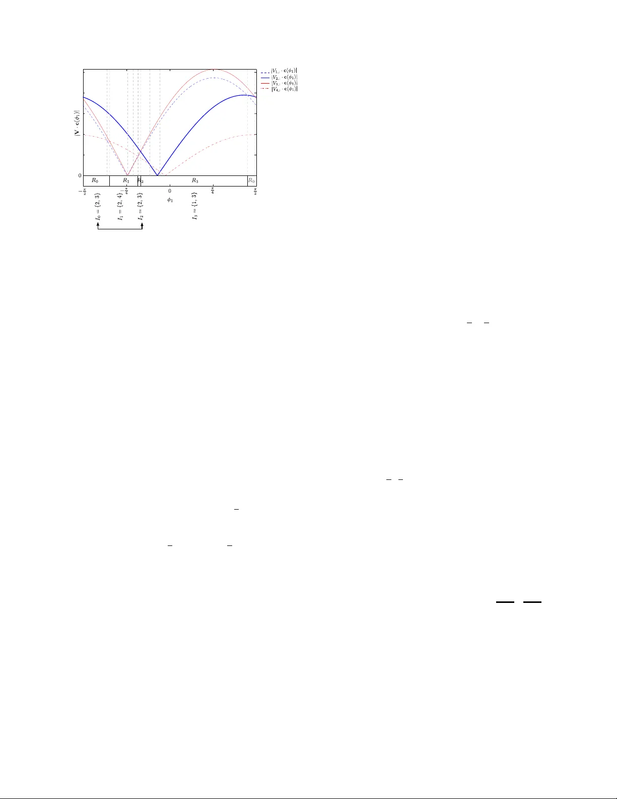
Sparse Principal Component of a Rank-deficient Matrix Megasthenis Asteris and Dimitris S. Papailiopoulos Department of Electrical Engineering Univ ersity of Southern California Los Angeles, CA 90089 USA Email: { asteris, papailio } @usc.edu George N. Karystinos Department of Electronic and Computer Engineering T echnical Univ ersity of Crete Chania, 73100, Greece Email: karystinos@telecom.tuc.gr Abstract —W e consider the problem of identifying the sparse principal component of a rank-deficient matrix. W e introduce auxiliary spherical variables and prov e that there exists a set of candidate index-sets (that is, sets of indices to the nonzero elements of the vector argument) whose size is polynomially bounded, in terms of rank, and contains the optimal index- set, i.e. the index-set of the nonzero elements of the optimal solution. Finally , we develop an algorithm that computes the optimal sparse principal component in polynomial time for any sparsity degree. I . I N T RO D U C T I O N Principal component analysis (PCA) is a well studied, popu- lar tool used for dimensionality reduction and lo w-dimensional representation of data with applications spanning many fields of science and engineering. Principal components (PC) of a set of “observ ations” on some N v ariables capture orthog- onal directions of maximum v ariance and offer a Euclidean- distance-optimal, low-dimensional visualization that -for many purposes- con veys sufficient amount of information. W ithout additional constraints, the PCs of a data set can be computed in polynomial time in N , using the eigen value decomposition. One disadv antage of the classical PCA is that, in general, the extracted eigen vectors are expected to hav e nonzero elements in all their entries. Ho wev er , in many applications sparse vectors that maximize v ariance are more fa vorable. Sparse PCs can be less complicated to interpret, easier to compress, and cheaper to store. Thus, if the application requires it, then some of the maximum v ariance property of a PC may be slightly traded for sparsity . T o mitigate the fact that PCA is oblivious to sparsity requirements, an additional cardinality constraint needs to be introduced to the initial variance maximization objectiv e. The sparsity aware flav or of PCA, termed spar se PCA , inarguably comes at a higher cost: sparse PCA is an NP-Hard problem [9]. T o approximate sparse PCA v arious methods hav e been introduced in the literature. Initially , factor rotation techniques that extract sparse PCs were used in [7], [4]. Straightforward thresholding of PCs was presented in [3] as a computationally light means for obtaining sparsity . Then, a modified PCA technique based on the LASSO was introduced in [5]. In [13] an elaborate nonconv ex regression-type optimization approach combined with LASSO penalty was used to approximately tackle the problem. A noncon ve x technique, locally solv- ing difference-of-con vex-functions programs was presented in [12]. Semidefinite programming (SDP) was used in [1], [14], while [15] augmented the SDP approach with an extra greedy step that offers fav orable optimality guarantees under certain suf ficient conditions. The authors of [10] considered greedy and branch-and-bound approaches, further explored in [11]. Generalized po wer methods using conv ex programs were also used to approximately solve sparse PCA [6]. A sparse- adjusted deflation procedure was introduced in [8] and in [2] optimality guarantees were shown for specific types of cov ariance matrices under thresholding and SDP relaxations. Our Contribution: In this work we pro ve that the sparse principal component of a matrix C can be obtained in poly- nomial time under a new sufficient condition: when C can be written as a sum of a scaled identity matrix plus an update, i.e. C = σ I N + A , and the rank of the update A is not a function of the problem size. 1 Under this condition, we show that sparse PCA is polynomially solvable, with the exponent being only a linear function of the rank. This result is possible after introducing auxiliary spherical variables that “unlock” the low-rank structure of A . The lo w-rank property along with the auxiliary variables enable us to scan a constant dimensional space and identify a polynomial number of candidate sparse vectors. Interestingly , we can sho w that the optimal vector always lies among these candidates and a polynomial time search can always retrie ve it. I I . P RO B L E M S TA T E M E N T W e are interested in the computation of the real, unit-length, and at most K -sparse principal component of the N × N nonnegati ve definite matrix C , i.e. x opt 4 = arg max x ∈ S N K x T Cx (1) where S N K 4 =  x ∈ R N : k x k = 1 , card ( x ) ≤ K  . Interest- ingly , when C can be decomposed as a low-rank update of a constant identity matrix, i.e. C = σ I N + A where σ ∈ R , I N is the N × N identity , and A is a nonne gativ e definite matrix 1 If σ = 0 , then we simply have a low-rank matrix C . with rank D , then x T Cx = σ k x k 2 + x T Ax . Therefore, the optimization (1) can always be rewritten as x opt = arg max x ∈ S N K x T Ax (2) where the new matrix A has rank D . Since A is a nonnegativ e definite matrix, it can be decomposed as A = VV T where V 4 = [ v 1 v 2 · · · v D ] and problem (1) can be written as x opt = arg max x ∈ S N K x T VV T x = arg max x ∈ S N K   V T x   . (3) In the following, we show that when D is not a function of N , (1) can be solved in time O ( poly ( N )) . I I I . R A N K - 1 A N D R A N K - 2 O P T I M A L S O L U T I O N S Prior to presenting the main result for the general rank D case, in this section we provide insights as to why sparse PCA of rank deficient matrices can be solved in polynomial time, along with the first nontri vial case of polynomial solvability for rank- 2 matrices A . A. Rank- 1 : A motivating example In this case, A has rank 1 , V = v , and (3) becomes x opt = arg max x ∈ S N K   v T x   = arg max x ∈ S N K      N X i =1 v i x i      . (4) It is trivial to observe that maximizing (4) can be done by distributing the K nonzero loadings of x to the K absolutely largest values of v , index ed by set I . Then, the optimal solution x opt has the following K nonzero loadings x opt , I = v I k v I k . (5) where x opt , I denotes the set of elements of x opt index ed by I and x opt ,i = 0 for all i / ∈ I . The leading complexity term of this solution is determined by the search for the K largest element of v , which can be done in time O ( N ) [16]. Therefore, the rank- 1 -optimal solution can be attained in time that is linear in N . B. Rank-2: Introducing spherical variables In this case, V is an N × 2 matrix. A key tool used in our subsequent de velopments is a set of auxiliary spherical variables. For the rank- 2 case, we introduce a single phase variable φ ∈  − π 2 , π 2  and define the polar vector c ( φ ) 4 =  sin φ cos φ  (6) which lies on the surf ace of a radius 1 circle. Then, from Cauchy-Schwartz Inequality we obtain   c T ( φ ) V T x   ≤ k c ( φ ) kk V T x k = k V T x k (7) with equality if and only if c ( φ ) is parallel to V T x . Therefore, finding x that maximizes k V T x k in (3) is equiv alent to obtaining x of the ( x , φ ) pair that maximizes   c T ( φ ) V T x   . Initially , this re writing of the problem might seem unmoti- vated, howe ver in the following we sho w that the use of c ( φ ) unlocks the lo w-rank structure of V and allows us to compute the sparse PC of A by solving a polynomial number of rank- 1 instances of the problem. W e continue by restating the problem in (3) as max x ∈ S N K k V T x k = max x ∈ S N K max φ ∈ ( − π 2 , π 2 ]   c T ( φ ) V T x   = max φ ∈ ( − π 2 , π 2 ] max x ∈ S N K | c T ( φ ) V T | {z } v T ( φ ) x | . (8) If we fix φ , then the internal maximization problem max x ∈ S N K   v T ( φ ) x   (9) is a rank- 1 instance, for which we can determine in time O ( N ) the optimal index-set I ( φ ) corresponding to the indices of the K absolutely largest elements of v ( φ ) = V c ( φ ) . Howe ver , why should φ simplify the computation of a solution? The intuition behind the polar vector concept is that ev ery element of Vc ( φ ) =    V 1 , 1 sin φ + V 1 , 2 cos φ . . . V N , 1 sin φ + V N , 2 cos φ    (10) is actually a continuous function of φ , i.e. a curve in φ . Hence, the K absolutely largest elements of Vc ( φ ) at a giv en point φ are functions of φ . Due to the continuity of the curv es, we expect that the index set I ( φ ) will retain the same elements in an area “around” φ . Therefore, we expect the formation of regions, or “cells” on the φ domain, within which the indices of the K absolutely largest elements of v ( φ ) remain unaltered. A sorting (i.e., an I -set) might change when the sorting of the amplitudes of two element in v ( φ ) changes. This occurs at points φ , where these two absolute values become equal, that is, points where two curv es intersect. Finding all these intersection points , is sufficient to determine cells and construct all possible candidate I -sets. Among all candidate I -sets, lies the set of indices corresponding to the optimal K -sparse PC. Exhausti vely checking the I -sets of all cells, suffices to retrieve the optimal. Surprisingly , the number of these cells is exactly equal to number of possible intersections among the amplitudes of v ( φ ) , which is exactly equal to 2  N 2  = O  N 2  , counting all possible combinations of element pairs and sign changes. Before we proceed, in Fig. 1 we illustrate the cell partition- ing of the φ domain, where we set N = 4 and K = 2 and plot the magnitudes of the 4 curves that originate from the 4 rows of Vc ( φ ) . Cells (interv als) are formed, within which the sorting of the curves does not change. The borders of cells are denoted by vertical dashed lines at points of curve intersections. Our approach creates 12 cells which exceeds the total number of possible index-sets, howe ver this is not true for greater values of N . Moreo ver , we use R i regions to denote the sorting changes with respect to only the K -largest curves. These regions is an interesting feature that might yet decrease the number of cells we need to check. Howe ver , due to lack of space we are not exploiting this interesting feature here. - p i/2 - p i/4 0 p i/4 p i/2 0 0.2 0.4 0.6 0.8 1 S R V M - Ra n k 2 S e r ia l A l go r i t h m  1 |V  c(  ) | |V 1,: c(  ) | |V 2,: c(  ) | |V 3,: c(  ) | |V 4,: c(  ) | Fig. 1. N = 4 , K = 2 , rank- 2 case: Cells on the φ domain. C. Algorithmic Developments and Complexity Our goal is the construction of all possible candidate K - sparse vectors, determined by the index-sets of each cell on the φ domain. This is a two step process. First we need to identify cell borders, and then we ha ve to determine the index sets associated with these cells. Algorithmic Steps: W e first determine all possible inter- sections of curve pairs in v ( φ ) . Any pair { i, j } of distinct elements in v ( φ ) is associated with two intersections: v i ( φ ) = v j ( φ ) and v i ( φ ) = − v j ( φ ) . Solving these two equations with respect to φ , determines a possible point where a ne w sorting of the K -largest values of v ( φ ) might occur . Observe that at an intersection point, the two values v i ( φ ) , v j ( φ ) are absolutely the same. Exactly on the point of intersection, all but 2 (the i th and j th) coordinates of a candidate K sparse vector can be determined by solving a rank 1 instance of the problem. Howe ver , we are left with ambiguity with respect to 2 coordinates i and j that needs to be resolved. T o resolve this ambiguity , we can visit the “outermost” point of the φ domain, that is, π 2 . There, due to the continuity of v i ( φ ) and ± v j ( φ ) , the sortings within the two cells defined by the two intersections, will be the identical, or opposite sortings of v i  π 2  and ± v j  π 2  , depending on whether v i ( φ ) and ± v j ( φ ) are both positiv e, or negativ e at the intersection point, respectiv ely . Having described how to resolve ambiguities, we hav e fully described a way to calculate the I -set at any intersection point. Apparently , all intersection points, that is, all  N 2  pairwise combinations of elements in v ( φ ) , ha ve to be examined to yield a corresponding I -set. Computational Complexity: A single intersection point can be computed in time O (1) . At a point of intersection, we hav e to determine the K -th order element of the absolute v alues of v ( φ ) and the K − 1 elements lar ger than that, which can be done in time O ( N ) . Resolving an ambiguity costs O (1) . So in total, finding a single I -set costs O ( N ) . Constructing all candidate I -sets requires examining all 2  N 2  points, implying a total construction cost of 2  N 2  × O ( N ) = O  N 3  . I V . T H E R A N K - D O P T I M A L S O L U T I O N In the general case, V is a N × D matrix. In this section we present our main result where we prove that the problem of identifying the K -sparse principal component of a rank- D matrix is polynomially solv able if the rank D is not a function of N . The statement is true for any value of K (that is, ev en if K is a function of N ). Our result is presented in the form of the following proposition. The rest of the section contains a constructiv e proof of the proposition. Proposition 1: Consider a N × N matrix C that can be written as a rank- D update of the identity matrix, that is, C = σ I N + A (11) where σ ∈ R and A is a rank- D symmetric positive semidef- inite matrix. Then, for any K = 1 , 2 , . . . , N , the K -sparse principal component of A that maximizes x T Cx (12) subject to the constraints k x k = 1 and card ( x ) ≤ K can be obtained with complexity O ( N D +1 ) . 2 W e be gin our constructi ve proof by introducing the spherical coordinates φ 1 , φ 2 , . . . , φ D − 1 ∈ ( − π 2 , π 2 ] and defining the spherical coordinate vector φ i : j M = [ φ i , φ i +1 , . . . , φ j ] T , (13) the hyperpolar vector c ( φ 1: D − 1 ) 4 =          sin φ 1 cos φ 1 sin φ 2 cos φ 1 cos φ 2 sin φ 3 . . . cos φ 1 cos φ 2 . . . sin φ D − 1 cos φ 1 cos φ 2 . . . cos φ D − 1          , (14) and set Φ 4 =  − π 2 , π 2  . Then, similarly with (8) and due to Cauchy-Schwartz Inequality , our optimization problem in (3) is restated as max x ∈ S N K k V T x k = max x ∈ S N K max φ 1: D − 1 ∈ Φ D − 1   x T V c ( φ 1: D − 1 )   . (15) Hence, to find x that maximizes k V T x k in (3), we can equi v- alently find the ( x , φ ) pair that maximizes   x T Vc ( φ 1: D − 1 )   . W e interchange the maximizations in (15) and obtain max x ∈ S N K k V T x k = max φ 1: D − 1 ∈ Φ D − 1  max x ∈ S N K | x T V c ( φ 1: D − 1 ) | {z } v 0 ( φ 1: D − 1 ) |  . (16) For a given point φ 1: D − 1 , V c ( φ 1: D − 1 ) is a fixed vector and the internal maximization problem max x ∈ S N K   x T V c ( φ 1: D − 1 )   = max x ∈ S N K    x T v 0 ( φ 1: D − 1 )    (17) is a rank- 1 instance. That is, for any given point φ 1: D − 1 , we can determine the optimal set I ( φ 1: D − 1 ) of the nonzero elements of x as the set of the indices of the K largest elements of vector | V c ( φ 1: D − 1 ) | . T o gain some intuition into the purpose of inserting the second v ariable φ 1: D − 1 , notice that every element of ± Vc ( φ 1: D − 1 ) is actually a continuous function of φ 1: D − 1 , a D -dimensional hypersurface and so are the elements of | Vc ( φ 1: D − 1 ) | . When we sort the elements of | Vc ( φ 1: D − 1 ) | at a giv en point φ 1: D − 1 , we actually sort the hypersurfaces at point φ 1: D − 1 according to their magnitude. The key ob- servation in our algorithm, is that due to the continuity of the hypersurf aces in the Φ D − 1 hypercube, we expect that in an area “around” φ 1: D − 1 the hypersurfaces will retain their magnitude-sorting. So we expect the formation of cells in the Φ D − 1 hypercube, within which the magnitude-sorting of the hypersurfaces will remain unaltered, irrespecti vely of whether the magnitude of each h ypersurface changes. Moreo ver , ev en if the sorting of the hypersurfaces changes at some point around φ 1: D − 1 it is possible that the I does not change. So we expect the formation of regions in the Φ D − 1 hypercube which expand ov er more than one cells and within which the I -set remains unaltered, even if the sorting of the hypersurfaces changes. If we can efficiently determine all these cells (or even better regions) and obtain the corresponding I -sets, then the set of all candidate index-sets may be significantly smaller than the set of all  N K  possible index-sets. Once all the candidate I -sets hav e been collected, I opt and x opt will be determined through exhausti ve search among the candidate sets. In (17) we observed that at a giv en point φ 1: D − 1 the maxi- mization problem resembles the rank- 1 case and consequently , the I -set at φ 1: D − 1 consists of the indices of the K largest elements of | Vc ( φ 1: D − 1 ) | . Motiv ated by this observ ation, we define a labeling function I ( · ) that maps a point φ 1: D − 1 to an index-set I ( V N × D ; φ 1: D − 1 ) M = arg max I X i ∈ I |  Vc ( φ 1: D − 1 )  i | . (18) Then, each point φ 1: D − 1 ∈ Φ D − 1 is mapped to a candidate index-set and the optimal index-set I opt belongs to I tot ( V N × D ) M = [ φ 1: D − 1 ∈ Φ D − 1  I ( V N × D ; φ 1: D − 1 )  . (19) In the follo wing, we (i) show that the total number of candidate index-sets is |I ( V N × D ) | ≤ b D − 1 2 c X d =0  N D − 2 d  D − 2 d  D 2  − d  2 D − 1 − 2 d = O ( N D ) and (ii) de velop an algorithm for the construction of I ( V N × D ) with complexity O ( N D +1 ) . The labeling function is based on pair-wise comparisons of the elements of Vc ( φ 1: D − 1 ) while each element of | V N × D c ( φ 1: D − 1 ) | is a continuous function of φ 1: D − 1 , a D - dimensional hypersurface, and any point φ 1: D − 1 is mapped to an index-set I which is determined by comparing the magnitudes of these hypersurfaces at φ 1: D − 1 . Due to the continuity of hypersurfaces, the inde x-set I does not change in the “neighborhood” of φ 1: D − 1 . A necessary condition for the I set to change is two of the hypersurfaces to change their magnitude ordering. The switching occurs at the intersection of two hypersurfaces where we hav e    Vc ( φ 1: D − 1 )  i   =    Vc ( φ 1: D − 1 )  j   , i 6 = j, which yields φ 1 = tan − 1 − ( V i, 2: D ∓ V j, 2: D ) T c ( φ 2: D − 1 ) V i, 1 ∓ V j, 1 ! . (20) Functions φ 1 = tan − 1  − ( V i, 2: D − V j, 2: D ) T c ( φ 2: D − 1 ) V i, 1 − V j, 1  and φ 1 = tan − 1  − ( V i, 2: D + V j, 2: D ) T c ( φ 2: D − 1 ) V i, 1 + V j, 1  determine ( D − 1) - dimensional hypersurfaces S ( V i, : ; V j, : ) and S ( V i, : ; − V j, : ) , respectiv ely . Each h ypersurface partitions Φ D − 1 into two regions. For con venience, in the following we use a pair { i, j } to denote the rows of matrix V N × D , that originate hypersurface S  i | i | V | i | , : ; j | j | V | j | , :  . Moreover , we allow i and j to be negati ve in order to encapsulate the information about the sign with which each ro w participates in the generation of hypersurface S , i.e. { i, j } 7→ S  i | i | V | i | , : ; j | j | V | j | , :  , (21) where i, j ∈ {− N , . . . , − 1 , 1 , . . . , N } , | i | 6 = | j | . Let { i 1 , i 2 , . . . , i D } ⊂ { 1 , 2 , . . . , N } where { i 1 , i 2 , . . . , i D } is one among the  N D  size- D subsets of { 1 , 2 , . . . , N } . Then, by keeping i 1 fixed (where i 1 is arbitrarily selected, say i 1 is the minimum among i 1 , i 2 , . . . , i D ) and assign- ing signs to i 2 , i 3 , . . . , i D we can generate 2 D − 1 sets of the form { i 1 , ± i 2 , . . . , ± i D } . Hence, we can create totally  N D  2 D − 1 such sets which we call J 1 , J 2 , . . . , J ( N D ) 2 D − 1 . W e can show (the proof is omitted due to lack of space) that, for any l = 1 , 2 , . . . ,  N D  2 D − 1 , the  D 2  hypersurfaces S  i | i | V | i | , : ; j | j | V | j | , :  that we obtain for { i, j } ⊂ J l hav e a single common intersection point ˆ φ ( J l ) which “leads” at most  D b D 2 c  cells. Each such cell is associated with an inde x-set in the sense that I ( V N × D ; φ 1: D − 1 ) is maintained for all φ 1: D − 1 in the cell. In other words, the I -set associated with all points φ 1: D − 1 in the interior of the cell is the same as the I -set at the leading v ertex. In fact, the actual sorting of | Vc ( φ 1: D − 1 ) | for all points in the interior of the cell is the same as the sorting at the leading vertex and the I -set may characterize a greater area that includes many cells. In addition, we can show that examination of all such cells is sufficient for the computation of all index-sets that appear in the partition of Φ D − 1 and ha ve a leading verte x. W e collect all index-sets into I ( V N × D ) and observe that I ( V N × D ) can only be a subset of the set of all possible  N K  index-sets. In addition, since the cells are defined by a leading verte x, we conclude that there are at most  N D  D b D 2 c  2 D − 1 cells. W e finally note that there exist cells that are not associ- ated with an intersection-vertex. W e can show that such cells can be ignored unless they are defined when φ D − 2 = π 2 . In the latter case, we just have to identify the cells that are determined by the reduced-size matrix V N × ( D − 2) ov er the hypercube Φ D − 3 . Hence, I tot ( V N × D ) = I ( V N × D ) ∪ I tot ( V N × ( D − 2) ) and, by induction, I tot ( V N × d ) = I ( V N × d ) ∪ I tot ( V N × ( d − 2) ) , 3 ≤ d ≤ D , which implies that I tot ( V N × D ) = I ( V N × D ) ∪ I ( V N × ( D − 2) ) ∪ . . . ∪ I ( V N × ( D − 2 b D − 1 2 c ) ) = b D − 1 2 c [ d =0 I ( V N × ( D − 2 d ) ) . (22) As a result, the cardinality of I tot ( V N × D ) is |I tot ( V N × D ) | ≤ |I ( V N × D ) | + |I ( V N × ( D − 2) ) | + . . . + |I ( V N × ( D − 2 b D − 1 2 c ) ) | ≤  N D  D j D 2 k  2 D − 1 +  N D − 2  D − 2 j D 2 k − 1  2 D − 3 + . . . +  N D − 2 b D − 1 2 c  D − 2 b D − 1 2 c j D 2 k − j D − 1 2 k  2 D − 1 − 2 b D − 1 2 c = j D − 1 2 k X d =0  N D − 2 d  D − 2 d j D 2 k − d  2 D − 1 − 2 d = O ( N D ) . (23) It remains to show how I ( V N × D ) is constructed. As already mentioned, there are in total  N D  2 D − 1 inter- section points which can all be blindly e xamined. For an y l = 1 , 2 , . . . ,  N D  2 D − 1 , the cell leading verte x ˆ φ ( J l ) is computed ef ficiently as the intersection of D − 1 hypersurfaces, i.e. the unique solution of    V i 1 , 1: D ∓ V i 2 , 1: D . . . V i 1 , 1: D ∓ V i D , 1: D    c ( φ 1: D − 1 ) = 0 ( D − 1) × 1 , (24) which is obtained in time O (1) with respect to N . After ˆ φ ( J l ) has been computed, we have to identify the index-sets associated with the cells that originate at ˆ φ ( J l ) by calling the labeling function I ( V N × D ; ˆ φ ( J l )) which marks the K ele- ments of the I -set, i.e. the indices of the K largest elements of | Vc ( ˆ φ ( J l )) | , l = 1 , 2 , . . . ,  N D  2 D − 1 . Since ˆ φ ( J l ) constitutes the intersection of D hypersurfaces that correspond to the D elements of ˆ φ ( J l ) , the corresponding values in | Vc ( ˆ φ ( J l )) | equal each other . If the K lar gest v alues in | Vc ( ˆ φ ( J l )) | contain D l values that correspond to the D elements of J l , then we can blindly examine all  D D l  cases of index-sets to guarantee that all actual inde x-sets are included. The term  D D l  is maximized for D l =  D 2  , hence at most  D b D 2 c  index-sets correspond to intersection point ˆ φ ( J l ) . The complexity to build I ( V N × D ) results from the parallel examination of  N D  2 D − 1 intersection points while worst- case complexity O ( N ) +  D b D 2 c  is required at each point for the identification of the corresponding index-sets. The term O ( N ) corresponds to the cost required to determine the K th-order element of | Vc ( ˆ φ ( J l )) | in an unsorted array . Consequently , the worst-case complexity to b uild I ( V N × D ) becomes  N D  2 D − 1 ×  O ( N ) +  D b D 2 c   = O ( N D +1 ) . Finally , we recall that the cardinality of I tot ( V N × D ) is upper bounded by O ( N D ) and conclude that the ov erall complexity of our algorithm for the e valuation of the sparse principal component of VV T is upper bounded by O ( N D +1 ) . V . C O N C L U S I O N S W e considered the problem of identifying the sparse prin- cipal component of a rank-deficient matrix. W e introduced auxiliary spherical variables and proved that there exists a set of candidate index-sets whose size is polynomially bounded, in terms of rank, and contains the optimal inde x-set, i.e. the index-set of the nonzero elements of the optimal solution. Finally , we de veloped an algorithm that computes the optimal sparse principal component in polynomial time. Our proposed algorithm stands as a constructive proof that the computation of the sparse principal component of a rank-deficient matrix is a polynomially solvable problem. R E F E R E N C E S [1] A. d’ Aspremont, L. El Ghaoui, M. I. Jordan, and G. R. G. Lanckriet, “ A direct formulation for sparse PCA using semidefinite programming, ” SIAM Review , 49(3):434-448, 2007. [2] A. A. Amini and M. W ainwright, “High-dimensional analysis of semidefi- nite relaxations for sparse principal components, ” The Annals of Statistics , 37(5B):2877-2921, 2009. [3] J. Cadima and I. T . Jolliffe, “Loadings and correlations in the interpreta- tion of principal components, ” Journal of Applied Statistics , 22:203-214, 1995. [4] I. T . Jolliffe, “Rotation of principal components: choice of normalization constraints, ” Journal of Applied Statistics , 22: 29-35, 1995. [5] T . Jollif fe, N. T . T rendafilov , and M. Uddin, “ A modified principal component technique based on the LASSO, ” Journal of Computational and Graphical Statistics , vol 12:531-547, 2003. [6] M. Journ ´ ee, Y . Nesterov , P . Richt ´ arik, and R. Sepulchre, “Generalized power method for sparse principal component analysis, ” 2008 [7] H. F . Kaiser , “The v arimax criterion for analytic rotation in factor analysis, ” Psychometrika , 23(3):187-200, 1958. [8] L. Mackey , “Deflation methods for sparse pca, ” Advances in Neural Information Processing Systems , 21:1017-1024, 2009. [9] B. Moghaddam, Y . W eiss, and S. A vidan, “Generalized spectral bounds for sparse LD A, ” in Proc. International Conference on Machine Learning , 2006a. [10] B. Moghaddam, Y . W eiss, and S. A vidan, “Spectral bounds for sparse PCA: exact and greedy algorithms, ” Advances in Neural Information Pr ocessing Systems , 18, 2006b . [11] B. Moghaddam, Y . W eiss, and S. A vidan, “Fast Pixel/Part Selection with Sparse Eigen vectors, ” in Pr oc. IEEE 11th International Confer ence on Computer V ision (ICCV 2007) , pp. 1-8, 2007. [12] B. K. Sriperumbudur , D. A. T orres, and G. R. G. Lanckriet, “Sparse eigen methods by DC programming, ” in Pr oc. 24th International Con- fer ence on Machine learning , pp. 831-838, 2007. [13] H. Zou, T . Hastie, and R. Tibshirani, “Sparse Principal Component Analysis, ” J ournal of Computational & Graphical Statistics , 15(2):265- 286, 2006. [14] Y . Zhang, A. d’ Aspremont, and L. El Ghaoui, “Sparse PCA: Con vex Relaxations, Algorithms and Applications, ” to appear in Handbook on Semidefinite, Cone and P olynomial Optimization . Preprint on ArXi v: 1011.3781v2 [math.OC]/ [15] A. d’ Aspremont, F . Bach, and L. El Ghaoui, “Optimal solutions for sparse principal component analysis, ” Journal of Machine Learning Resear ch , 9: 1269-1294, 2008. [16] T . H Cormen, C. E. Leiserson, R. L. Rivest, and C. Stein, Intr oduction to Algorithms , 2nd ed. MIT Press 2001, Part II, Chapter 9.