Complexity Analysis of Vario-eta through Structure

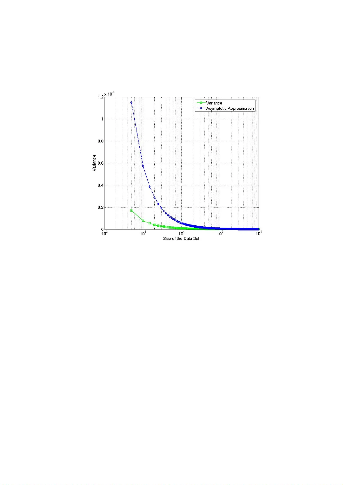
Complexity Analysis of Vario-eta through Structure Alejandro Chi nea and Elka K orutcheva Departamento de Física Fundamental , Facultad de Ci encias UNED, Paseo Senda del Rey nº9, 28040-Madrid - Spain Abstract. Graph-based represe ntations of images have recen tly acquired an important role for classification purpos es wit hin the context of machine learning approaches. The und erlying idea is to consider that relev ant information of an image is implicit ly encoded into the relationships between more basic entities that compose by themselves the whole image. The classification problem is then reformulat ed in terms of an optimization p roblem usually solved by a gradient-based search procedure. Vario-eta through structure is an approximate second order stoch astic optimization techniqu e that achieves a good trade-off between speed of convergence and the computational effort required. However, the robustne ss of this technique for larg e scale problems has not been yet assessed. In this paper we firstl y provide a theoretical justification of the assumptions m ade by this optimization procedure. Secondly, a complexity analysis of the algorithm is performed to prove its suitabili ty for large scale learning problems. Keywords: image anal ysis, machine learning, analyti c combinatorics . 1 Introductio n In general, an i mage can alwa ys be interprete d as a combinat ion or mixt ure of simple r entities. The complexity of imag e analysis is usually due to the difficulties involved in discovering the nature of th e relationship of these constitu ent elements. Surprisingly, species ranging from insects to mammals so lve visual recog nition problems extremely well. They have an inherent cap acity to represent the tem poral structure of experience, such inform ation representation making it possible for an animal to adapt its behaviour to the temporal structure of an event in its behavioural space [9]. In particular, humans can recognize an object from a single prese ntation of it s image without the necessity of integ rating information ov er multiple time steps as would be required by classi c machine learning paradigms. Indeed, t he human perce ption system organizes in formation by using cohesive st ructures [13, 14]. Specificall y, the human perception process always tries to assign structure to any perceptual information based upon prev iously stored know ledge stru ctures (e.g. an imag e is recognized by identifying its structural comp onents). Th is fact validates a well-known premise from the machine learning field that states that th e structure of an entity is very importan t for both classifi cation and descripti on. Furtherm ore, these ideas have motivat ed the development of a new branch of m achine learning algorit hms [7,8,10, 15,17,19] that use structured representations (i .e. graph-base d represent ations) of dat a for both classification and regression tasks i nstead of classic vector-based represe ntations. For instance, an image can be represented by its region adjacency graph [1, 16] (see figure 1) which is extracted from the image by associati ng a node to each h omogeneous region, and li nking the no des related to adjacent regi ons. In the re gion adjacency representation each node is labelled by a real vector, t hat represents features of the region (position, area, mean colour, texture, etc.). Thus, not only perceptual features of the image are captured with this representation bu t also its spatial arrangement. It is important to note that the notion of info rmation content is strongly lin ked to the notion of st ructure. Fig. 1. Example of a gr aph-based representation o f an artificial image us ing a region adjacen cy graph, each node of the graph is relate d to a homogeneous region of the image. Moreover, im age processing i s done on th e num erical representation of the image, i.e. a large matrix, therefore, t hese arrays can be enorm ous, and as soon as one deals with a sequenc e of images, such as in television or video appl ications, the vol ume of numerical data t hat must be processe d becomes im mense. Taking int o account these considerations it can be deduced that the classification of large image data sets is a difficult computation al task that becomes even more complex when dealing with structured representations of im ages. Ther efore, from a machin e learning point of view a great deal of resea rch has been devot ed to the developm ent of fast comput ation learning sche mes. In particul ar, for struct ured representat ions of dat a vario-eta through structure [3] has b een recently proposed as an efficient learning schem e offering a good trade-off b etween speed of convergence an d associated compu tational cost. Furtherm ore, this learni ng scheme ach ieves a rate of converge nce similar to a quasi-Newto n method at the com putational cost of a first orde r method, an d additionally, it offers the possibility of working in both sequential and in batch modes. The present paper explores the reliab ility of this approximate seco nd order stochastic gradient-b ased search optimi zation procedure for large scale learning problem s. The rest of the paper is organized as foll ows: in the next s ection, som e background t opics on the vario-eta gr adient-based opt imization t echnique are introduced. F urthermore, the assumptions made by thi s optimi zation procedure a re assessed from a theoretical point of view in order to check th eir reliability. Section 3 is devoted to the complexity an alysis of the algor ithm for structured domains. Specifically, the ge nerating funct ions of the rec ursions associated to this learning scheme are analysed from an analytic com b inatorics point of view. Section 4, is focused on t he practical applicati ons of th e complexity analysis performed in section 3. Finally, sect ion 5 provides a sum mary of the present study together wit h some concluding remarks. 2 Vario-eta Learning Rul e The problem of learning in b oth deterministic and probabilistic machine learning models is frequently form ulated in terms of param eter optim ization techniq ues. The optimi zation problem is usual ly expressed in t erms of the minimi zation of an e rror function E . This error is a function of the ad ap tive parameters of the mod el. One of the simplest techniques is gradi ent-search opti mization w hich is one which has bee n widely studie d. Here we investi gate an approxima te second order stochas tic gradient- search learning rule known as vario-eta [20]. 2.1 Mathem atical Descripti on Without a loss of generality, let us d enote as E(w) the error fu nction to be m inimized. In addition, let us suppose that we expr ess the parameters of our model in a vector w =[ w 1 ,w 2 ,w 3 ,….,w m ]. A perturbatio n of the error function around some point of the model parameters can be written as follows: E(w+ ∆ w) = E(w 1 + ∆ w 1 , w 2 + ∆ w 2, …., w m + ∆ w m ) . Considering t he Taylor expansi on of the err or function aro und the perturbation ∆ w we obtain: .......... ) ( ! 3 1 ) ( ! 2 1 ) ( ) ( ) ( 3 1 2 11 + ⎟ ⎟ ⎠ ⎞ ⎜ ⎜ ⎝ ⎛ ∆ ∂ ∂ + + ⎟ ⎟ ⎠ ⎞ ⎜ ⎜ ⎝ ⎛ ∆ ∂ ∂ + ∆ ∂ ∂ + = ∆ + ∑ ∑∑ = == m i i i m i m i i i i i w w E w w E w w E w E w w E (1) In the batch ve rsion of gradi ent-descent ap proach, we start with some initial guess of model parameters. Then, model paramet ers are updated iteratively usin g the entire data set. In the sequential [14, 15 ] version of gradien t descent, the error function gradient is e valuated for j ust one pattern (or a batch of patterns smal ler when compared to the size of the data set for t he case of the vario-eta learning rule ) at a time. Each updat e of model param eters can be viewed a s perturbations (i.e. noise) around the cur rent point give n by the m dimensi onal vector of m odel paramet ers. Let us assume a gi ven sequence of N distu rbance vectors ∆ w . Considering the error as a random vari able and ignorin g third and highe r order ter ms in express ion (1), the expectation of the error can be ex pressed as: ∑ = ∆ + ≅ N n n w w E N w E 1 ) ( 1 ) ( (2) Substituting the Taylor exp ansion of the error function in expression (2) and rearranging terms we obtain a series expans ion of the expectation of the error as a function of t he moment s of the random perturbations: ∑ ∑∑ < == ∂ ∂ ∆ ∆ + ∂ ∂ ∆ + ∂ ∂ ∆ + ≅ j i j i j i i m i m i i i i w w E w w w E w w E w w E w E 2 2 2 11 2 ) ( 2 1 ) ( ) ( (3) In addition, the weight in crement associated to the gr adient descent ru le is ∆ w i = - η g i . The third term of expression (3) c oncerning t he covariance can be ignored supposing that the elements of the di sturba nce vectors are uncorrelated over the inde x n. This is a plausi ble hypothesis gi ven th at patterns of the data set are selected randomly duri ng the optimi zation procedur e. Moreover, cl ose to a local minim um we can assume that 0 ≅ ∆ i w . Taking into account these consid erations the expectation of t he error is then given by: 2 2 1 2 2 2 2 1 2 ) ( 2 ) ( ) ( 2 1 ) ( ) ( i m i i i m i i w E g w E w E w w E w E ∂ ∂ + = ∂ ∂ ∆ + ≅ ∑ ∑ = = σ η (4) From equation (4), it is easy to dedu ce that the expected valu e of the error increases as the variance (represe nted by the symbol σ 2 ) of the gradients increases. This observation sug gests that the error function should be strongly penalized around such model param eters. Therefore, to cancel the noise term in the expected value of the error functi on the gradient de scent rule must be changed to ∆ w i = - η g i / σ ( g i ). This normali zation is know n as vario-eta a nd was propose d in [20] f or training neural networks. Specifically, the learn ing rate is renormalized by the stochasticity of the error gradie nt signals. 2.2 Virtues and Limitations of the Approximation Expression (4) was obtained unde r the hypothesis tha t the expectation of the perturbation s ∆ w i could be neglected near to a local minimum. To confirm the validity of this approxi mation, let us first ly express the expectation of the perturba tions ∆ w i in terms of the error gradien ts g i (using the expressi on of the gradient optimization update rule) : ∑ ∑ = = = = − − = − = ∆ N n n i i N n n i i i i i i i i i g N g g N g g g g g g g w 1 2 2 1 2 ) ( 1 ) ( 1 ) ( η σ η (5) (6) Substituting expression (6) (i.e. th e values of the first and second order moments of the error g radients) in ex pression (5) and rearranging, we get : 1 ) ,...., , , ( 1 ) ( 3 2 1 2 1 1 2 − − = − ⎟ ⎠ ⎞ ⎜ ⎝ ⎛ − = ∆ ∑ ∑ = = N i i i i N n n i N n n i i g g g g f N g g N w η η (7) In the previous expression , we introduced the multidimensional fun ction f . This function de pends on the error gradients obtai ned through N iteration steps. Furthermore, it is easy to show (see e xpr ession (7)) that t he minim um and maxim um values of the f unction are 1 a nd N respectively. Specifically, the function reaches its maximu m wh en the e rror gradie nts ar e identic al. ∑ ∑ ∑ ∑ = < = = + = ⎟ ⎠ ⎞ ⎜ ⎝ ⎛ = N n n i k n k i n i N n n i N n n i N i i i i g g g g g g g g g f 1 2 1 2 2 1 3 2 1 ) ( 2 1 ) ( ) ,...., , , ( (8) This fact is of particular interest as it implies that the error gradients must be identical through N iteration steps. Taking into accoun t that N represents the size of the batch, the probab ility of such event is N M − , where M is the total size of the training set. It is important to note that in the batch version of gradient descent M=N . Therefore, such event can be ignored as its prob ability can be co nsidered zero as in practice M>>N>>1 . Howeve r, numerical precision errors c ould make the contribution of the term (7) big enough to break the validity of the hypothesis. This scenario would cause oscillations of the error E during th e optimization procedure. Therefore, the approx imation is limited in practice by the precision of the machine; although their i mpact is minimal, taking into account the precision ach ieved by current 64 bi t platforms of modern com puters. Moreo ver, in order t o alleviate eventual numerical problems a small constant 0 < φ << 1 can be sum med to the standard de viation of the error gradie nts (e.g. φ = 10 -6 ) as suggested in [3]. 3 Compl exity Anal ysis From a computational point of view machine learning models that work with structured representations of data are intrinsically more complex than their v ector- based counterparts are . The fact of using struct ured representat ions of data is translated into a substantial gain in information content b ut also in an increase on computational complexity. Indee d, the principal drawback of t hese models is a n excessively expensive c omputational l earning phase. The learni ng rule studie d in the previous secti on was adapted an d expressed in a rec ursive form i n [3] for working with structured representations of data. The fact of expressing s uch calculations in a recursive form permitted a considerable redu ction in memory storage something fundamental for learning problems composed of huge dat a sets. In this section, a complexity analysis of such algorithm is perfor med using elements of the theory of an alytic combinatorics [4, 6]. The main objective o f analytic combinatorics is to p rovide quantitative pr edictions of th e properties of large combinatorial structures. This theory has e merged over recent deca des as an essential tool for the analysis of algo rithms and for the study of scientific models in many disciplines. Here, our intention is to study the asymptotic beh aviour of the learn ing rule to reduce its computational requ irements for larg e-scale learning problem s. To this end, in subsection 3.1, we firstly p rovide some background topics on analytic combinatorics. Afterwards, in subsection 3. 2 we model the algorithmic structure of the learning rule in terms of g enerating functions. Finally, in subsection 3.3 the singularities of the generating functions are an alysed aimed at obtaining an asymptoti c approximat ion of its coeffici ents for reducing the co mputational requirements associated to this learning rule. 3.1 The oretical Bac kground Let us introd uce some basic d efinitions to be used throu ghout the rest of this paper: Definition 3. 1.1: The ordina ry generating f unction of a seque nce n A is the form al power series: ∑ ∞ ≥ = 0 ) ( n n n z A z A (9) Generating functions are the central object of study of analytic combinatorics. Their algebraic structure directly reflects the structure of the underlying combinatorial object. Furthermore, they can be viewe d as analytic transfor mations in the complex plane and its singularities account for the as ymptotic rate of gr owth of function’s coefficients. In addition, the t heory elaborat es a collection of methods (e. g. singularity analysis or saddle po int method) by wh ich one can extract asymptotic counting informati on from generati ng functions . Definition 3.1.2: we let general ly ) ( ] [ z f z n denote the operation of extracting the coefficient of n z in the formal power series ∑ = n n z f z f ) ( ∫ ∑ + ∞ ≥ = = ⎟ ⎠ ⎞ ⎜ ⎝ ⎛ c n n n n n n dz z z f i f z f z 1 0 ) ( 2 1 ] [ π (10) In expressio n (10), Cauchy' s integral fo rm ula expresses coefficients of analytic functions as c ontour inte grals. Therefore, an appropriate use of Cauch y’s integral formula then makes it possible to estimate su ch coefficients by su itably selecting an appropriate contour of integration. 3.2 Vario-eta Generating Functi ons Generally speaking, an algorithm can be inte rpreted as a mathematical object that is built iteratively from a set of finite rules that work on finite data structures. Furthermore, they have an inherent com binatorial struct ure that can be modelled i n terms of gene rating functi ons. In the foll owing, we model the algorithm ic description of the vario-et a learning r ule in terms of generating f unctions. The algorithm ic description of the learni ng rule provi ded in [3] is com posed of t wo recurrences expresse d in matrix form. These two finite diffe rences equations accounted for the calcula tion of the mean and variance of the error gradients during the gradient-d escent optimization lo op. In order to simplify the no tation, let us write without a loss of generality such equations in a single variable form: n n n n n g b g a g + = − 1 ˆ ˆ ∑ = = ⇔ n k k n g n g 1 1 ˆ () 2 1 2 1 1 2 ˆ − − − − + = n n n n n n g g b a σ σ ∑ = − − = ⇔ n k n k n g g n 1 2 2 ) ˆ ( 1 1 σ (11) (12) The generating functions associated to the recurrences for the m ean and variance of the error gradie nts can be comput ed applying the trans formation (9) t o both sides of equations (11) and (12). Specifi cally, equation (1 2) was expressed o nly in term s of the averaged error gradients and their varianc e to eliminate its dep endency with the unknown gene rating functi on of the erro r gradients g(z). ∑∑ ∑ ∞ ≥ ∞ ≥ ∞ ≥ − + − = 00 0 1 1 ˆ ) 1 1 ( ˆ nn n n n n n n n z g n z g n z g ∑ ∑∑ ∑ ∑ ∞ ≥ − ∞ ≥ ∞ ≥ ∞ ≥ ∞ ≥ − − − + − − = 0 1 00 0 0 2 2 1 2 1 2 ˆ ˆ 2 ˆ 1 1 n n n n nn n n n n n n n n n n z g g n z g n z n z z σ σ σ (13) (14) After doing some algebra and using the c omplex con volution the orem [18], we obtain the following integral equations in the co mplex variable z for the generating functions of mean of error gradients ) ( ˆ z g and their variance ) ( 2 z σ respectively: ∫ − = dz z g z z z g ) ( ) 1 ( 1 ) ( ˆ ∫∫ − = + − c du u z g du u g d u i dz z z z z z ) / ( ˆ ) ( ˆ ) 1 ( 2 1 ) ( 1 ) ( ) 1 ( 2 2 π σ σ (15) (16) Despite we do not know the form of the generati ng function of t he error gradient s neither their counting sequence n g we can make reasonable hypothesis about their form turning into a probabilistic framework. More specifically, the coun ting sequence n g is the result of co mputing the error grad ient associated to a pattern randomly selected at iteration step n from the training set durin g the optimization loop. Therefore, we can c onsider each of them as n independent ra ndom vari ables. Furthermore, during the opt imization loop the parameters of the machine learning model are not updat ed, therefore the n inde pendent ra ndom variables re presenting the error gradients will be statisti cally equally distribu ted. It is important to note that th e machine learni ng model can be viewed as a functional of t he optimization pa rameters. Moreover, error gradien ts are calculated evaluating the fu nctional by using the patterns of the data set. Tak ing into account we are interested in large-scale learning problems the statistical distri bution of the av eraged error gradien ts n g ˆ will tend, by virtue of Laplace’s central-limit theorem, to a Gaus sian distribution at the extent the value of n increases. It is important to n ote that the valu e n represents the size of the data set for the case of batch l earning and the size of the batch of pat terns for sequential learning problems. Thus, its pr obab ility generating function will have the following e xpression: 2 2 2 1 ) ( ˆ z z e z g σ µ − ≅ (17) The complex funct ion ) ( ˆ z g is analytic for |z| < ¶ , it is also holom orphic (i.e. complex-differentiable), which is equ ivalent to saying that it is also an alytic. Additionally, it can b e proved that ) / 1 ( ˆ z g is also analytic. Moreover, the function under the contour integral of exp ression (16) will be an alytic in |z| < 1. Hence, by virtue of the C auchy’s residue theo rem this integral is zero as the contour o f integration d oes not contain any singularity (Null integral prop erty). Taking these considerations into account we can get a closed expression for ) ( 2 z σ as follows: 0 ) ( ) ( ) 1 ( 2 2 2 2 = − − dz z d z dz z d z z σ σ => ⎟ ⎟ ⎠ ⎞ ⎜ ⎜ ⎝ ⎛ ⎟ ⎠ ⎞ ⎜ ⎝ ⎛ − + + = z z z z 1 log 1 1 ) ( 2 σ (18) 3.3 Singul arity Anal ysis The basic principle of singularity anal ysis is the existence of a general correspondenc e between the asym ptotic expa nsion of a funct ion near it s dominant singularities and the asymptotic expansion of the function ’s coefficients. Specifically, the method is mainly based on Cauc hy's coefficient formula used i n conjunction wi th special contour s of integration kn own as Hankel cont ours [5]. Here we a re interested in obtaining a n asymptoti c expression for t he coefficients of the generat ing function obtained i n (18).Hence, t he fi rst step consist in expressing such coeffi cients as a contour int egral using t he Cauchy’s coe fficient form ula: ∫ ∫ ∫ ∫ ⎟ ⎠ ⎞ ⎜ ⎝ ⎛ − + + = = + + c n c n c n c n n dz z z z i dz z i dz z i dz z z i z z 1 log 1 2 1 1 2 1 1 2 1 ) ( 2 1 ) ( ] [ 1 1 2 2 π π π σ π σ (19) The second step is to express the contour integral (19) usi ng a Hankel contour. To this end, unde r the change of vari ables z = 1 + t/n , t he kernel 1 − − n z in the integral (19) transf orm asymptot ically into an e xponential. Usi ng the aforem entioned cha nge of variables in expression (19) together with a Hankel contou r we obtain: ∫ ∫ ∫ ∞ + − ∞ + − ∞ + − − ⎟ ⎠ ⎞ ⎜ ⎝ ⎛ + ⎟ ⎠ ⎞ ⎜ ⎝ ⎛ + + + ⎟ ⎠ ⎞ ⎜ ⎝ ⎛ + + ⎟ ⎠ ⎞ ⎜ ⎝ ⎛ + = ) 0 ( ) 0 ( ) 0 ( 1 2 / 1 / log 1 2 1 1 2 1 1 2 1 ) ( ] [ dt n t n t n t n i dt n t n i dt n t n i z z n n n n π π π σ (20) The contour and the associated rescaling cap ture the be haviour of t he function nea r its singularities, enabling co efficient estimation when n Ø ¶ . ∫ ∞ + − − − = Γ ) 0 ( ) ( 2 1 ) ( 1 dt e t i s t s π (21) Re-arranging terms and expressing the integr als in terms of the gamma function (see expression 21), we fi nally get t he asymptotic expansion f or the variance of the error gradien ts: n n n n z z n n γ γ σ σ ≅ − − ≅ = 3 2 2 2 2 1 1 ) ( ] [ (22) The result achieved by expression (22 ), where γ is the Euler number, is particularly interesting. It implies that for large enough values of n (data set size) we do not need to perform the iterative or th e direct calcu lation of the vari ance (see expression (1 2) ) as it can be ap proximated usi ng the above e xpression that i s dependent excl usively on the size of the data set (or the size of the batch for se quential learning). 4 Practical Results Expression (22 ) provides the law of asympt o tic growth of the co e fficients associated to the generati ng function de scribing the va riance of the avera ged error gra dients. Figure 2 shows the result of computing the variance of a random variable. That is it shows the result of averaging n uniformly distributed random v ariables in the interval [0,1] for value s of n (i.e. size of the data set ), ranging from 500 up to 1000,000 ( see the solid line style with squares) ag ainst the asymptotic approximation o btained in section 3 (see t he dashed line st yle using diam onds at the sam pling points ). Fig. 2. The variance of the av erage of n (i.e. size of the data se t) uniformly distributed random variables versus its asymptotic approximation… From inspection of the graph, it can be observed that the approximation works quite well for values of n bigger or equal to 50 ,000. For exam ple, at n = 49,50 0 the error between the real value and its approximation is less than 10 -5 . Similarly, fo r n = 5,000 the error is less than 1 0 -4 . These result s are of particular inte rest for huge data sets (i.e. n ¥ 10 6 ) where batch learning becom es im practical even for sophisticated gradient-based acceleration technique s like conjugate-gradients m ethods [2, 11] due to the mem ory storage requir ements and asso ciated com putational cost. Furthermore, these kinds of acceleration techniques are not available for sequentia l learning. In this regard, vario-eta offers the possibility of working in sequential and batch learning modes. Let us suppose that th e size of the data set is M , and let us denote by N the size of the batch. The converge nce of the learning ru le in a sequential learning scenario is always guaranteed by the Robb ins- Monro theorem [12] if the condition M>>N is satisfied. The refore, under t he hypothesi s of a huge value of M if we f urther impose the condition N>>1 th e asymptotic approximatio n (22) will hold, thu s we can obtain for a large-scale sequential learning pr oblem a speed of convergence of an approximate second order algorithm at an extremel y reduced comput ational cost. Nevertheless, it is important to note th at these theoretical results must be interpreted carefully as real -world data s ets usually cont ains correlated patterns that coul d break in certain cases the i ndependence assum ption made in se ction 3. Hence, pr oviding a more practical guideline fo r real-world data sets rem ains for future work. 5 Conclusion s In this paper, we have inve stigated the applicability of an approximate second order stochastic learni ng rule to large -scale learning pro blems. Throughout this paper we have referred to the conce pt of structured representations of data as a way of increase the information content o f a representatio n. In particular, within a machin e learning context we have describe d the advanta ges of grap h-based re presentation of images for classification purposes. H owever, this kind of re presentation re quires new l earning protocols abl e to deal not only with the in creased complexity asso ciated to the use of structured re presentations of informat ion but also wi th huge learni ng data sets. In this context, we have presented a m a thematical descript ion of the vari o-eta learning rule. We have also assessed through a detailed an alysis the reliability of its working hypo thesis. Moreover, we have pres en ted a careful complexity analysis of the algorithm aimed at understanding its as ymptotic properties. As a result of this analysis we deduced an asymptotic expressi on for the learning rule. Specifically, such an approxim ation achieves a considerable re duction on t he computational cost associated to the learning rule when d ealing with large-scale learning problems. Acknowledgments: The authors acknowledge the f inancial support by gr ant FIS 2009-9870 from the Spa nish Mini stry of Science a nd Innova tion. References 1. Bianchini, M., Gori, M, Sarti , L., Scarselli, F.: Recurs ive Processing of Cyclic Graphs. IEEE Transactions on Neural Networks 9 (17), pp. 10- 18 (2006) 2. Bishop, C.M.: Neural Networ ks for Pattern Recognition, Ox fo rd University Press, Oxford (1997) 3. Chinea, A.: Understanding the Principles of Recursive Neural Networks: A Generative Approach to Tackle Model Complexity. In: Alippi, C., Polycarpou, M., Panayiotou, C., Ellinas, G. (eds.) ICANN 2009. LNCS 5768, pp. 952-963. Springer, Heidelb erg (2009) 4. Comtet, L.: Advanced Combinatorics: The Ar t of Finite and Infinite Expansions. Reidel Publishing Company, Dordrecht (1974) 5. Flajolet, P., Odlyzko, A. M.: Singularity Analysis of Gener ating Functions. In: SIAM Journal on Algebraic and Discrete Methods 3,2 New York (1990) 6. Flajolet, P., Sedgewick R.: Analytic Co mbinatorics. Cambridge Univ ersity Pre ss, Cambridge (2009) 7. Frasconi, P., Gori, M ., Kuchler, A., Sperdutti, A .: A Field Guide to Dynamic al Recurrent Networks. In: Kolen, J., Kremer, S. (Eds), pp . 351-364. IEEE Press, Inc., New York (2001). 8. Frasconi, P., Gori, M, Sperduti, A.: A Gene ral Framework for Adaptive Processing of Data Structures. IEEE Transactions on Ne ural Networks 9 (5), pp. 768- 786 (1998) 9. Gallistel, C.R.: The Organization of Learning. MIT Press, Cambridge (1990) 10. Gori, M., Monfardini, G., Scarselli, L.: A New Model for Learn ing in Graph Domains. In: Proceedings of the 18 th IEEE International Joint Conferenc e on Neural Networks, pp. 729- 734, Montreal (2005). 11. Haykin, S.: Neural Networ ks: a Comprehensive Foundation. P rentice Hall, New Jersey (1999) 12. Kushner, H.J., Yi n, G. G.: Stochastic Approximati on Algorithms and Applications. Springer-Verlag, New York (1997) 13. Ley ton, M.: A Generative Theory of Shape. In: LNCS, vol 2145 , pp. 1-76. Springer-Verlag (2001) 14. Leyton, M.: Symmetry, Causality, Mi nd. MIT Press, Massachusetts (1992). 15. Mahé, P., Vert, J .-P. : Graph Kernels Base d on Tree Pat terns for Molecules. In: M achine Learning, 75(1), pp. 3-35 (2009) 16. Mauro, C. D., Diligenti, M., G ori, M, Ma ggini, M.: Similarity Learning for Graph-based Image Representations. In: Patt ern Recognition Letters , vol. 24, no. 8, pp . 115-1122, (2003) 17. Micheli, A., Sona, D., Sperduti, A.: Contextu al Processing of Structured Data b y Recursive Cascade Correlation. IEEE Transactions on Neur al Networks 15(6) (2004) 1396-1410 18. Oppenheim, A. V., Schaf er, R.: Discrete-Tim e Signal Processing. Prentice Hal l, New Jersey (1989) 19. Tsochantaridis, I., Hofmann, T., Joachims, T., Al tun, Y.: Support Vector Machine Learning for Interdependent and Structured Output Sp aces. In : Brodley, C. E. (Ed.), ICML’04: Twenty-first international conference on Mach ine Learning. ACM Press, New York (2004) 20.Zimmermann, H. G., Neuneier, R.: How to Tr ain Neural Networks. In: Orr, G.B., Müller, K.-R. (eds.): NIPS-WS 1996. LNCS, vol. 1524, pp. 395-399. Springer, Heid elberg (1998)