Evaluation of Martons Inner Bound for the General Broadcast Channel

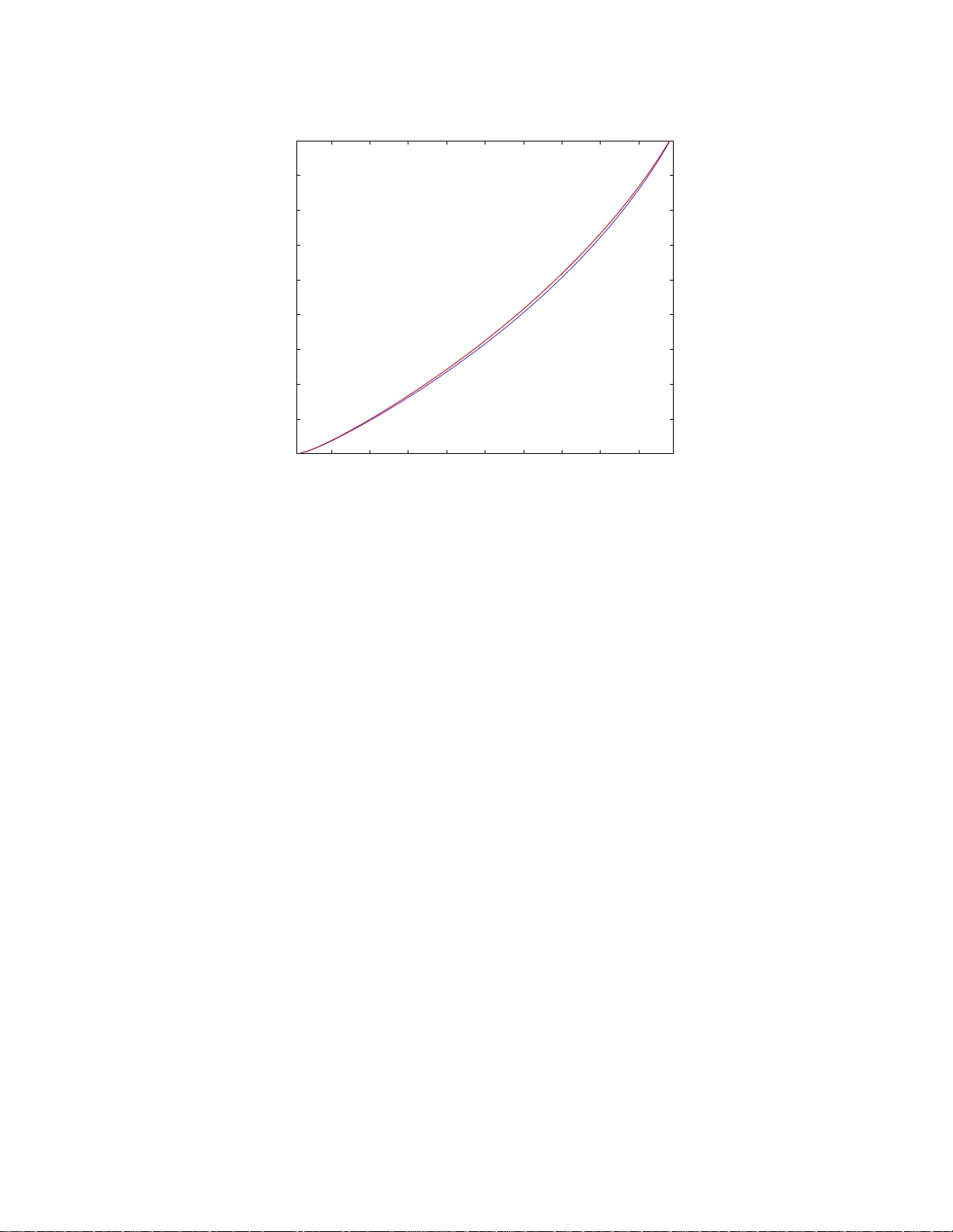
1 Ev aluation of Marton’ s Inner Bound for the General Broadcast Cha nnel Amin Aminzadeh Gohari and V enkat Anantharam Department of Electrical Engineering and Computer Science Univ ersity of California, Berkele y { aminzade, ananth } @eec s.berkeley.edu Abstract The best known inner b ound on the two-receiver gen eral br oadcast ch annel with out a commo n message is due to M arton [3]. This result was su bsequently generalized in [p. 391 , Problem 10(c ) 2] and [4] to broad cast chan nels with a common message. Howe ver the latter region is not compu table (except in certain spec ial cases) as no boun ds on the card inality of its au xiliary rando m variables exist. Nor is it e ven clear that the in ner bound is a closed set. The main obstacle in proving cardina lity boun ds is the fact tha t th e traditional use o f the Carath ´ eodory the orem, the main k nown tool for proving card inality bound s, does not yield a finite cardinality result. On e of the main contributions of this paper is the introdu ction of a new tool b ased on an identity th at relates th e second deriv ative of the Sh annon entr opy of a discrete random variable (under a certain p erturbatio n) to th e corr espondin g Fisher inform ation. In order to go beyo nd the traditional Car ath ´ eodory type arguments, we identify certain pr operties that the auxiliary rando m v ariab les correspond ing to the extrem e points of the inner boun d need to satisfy . These proper ties are then u sed to establish card inality bou nds on the auxiliary rando m variables of the inner bound , th ereby provin g th e c omputab ility of the region, and its closed ness. Lastly , we estab lish a conjectur e of [12] that Marton’ s inner boun d and the recen t outer b ound of Nair and El Gamal do no t match in gen eral. I . I N T R O D U C T I O N In this paper , we consider two-recei ver g eneral b roadcast channe ls. A two-receiver broadca st chann el is cha racterized b y the c onditional distribution q ( y , z | x ) where X is the input to the channe l an d Y and Z are the outputs of the channel at the two receiv e rs. Le t X , Y and Z den ote the a lphabet set of X , Y and Z respec ti vely . The transmitter wants to send a common mess age, M 0 , to both the receiv e rs a nd two priv ate messa ges M 1 and M 2 to Y a nd Z respectively . Assume that M 0 , M 1 and M 2 are mutua lly DRAFT 2 independ ent, and M i (for i = 0 , 1 , 2 ) is a uniform ran dom variable over set M i . The transmitter maps the mes sages into a codeword of length n using an en coding func tion ζ : M 0 × M 1 × M 2 → X n , and sends it over the broadcast ch annel q ( y , z | x ) in n times steps. The rec eiv e rs u se the deco ding functions ϑ y : Y n → M 0 × M 1 and ϑ z : Z n → M 0 × M 2 to map the ir receiv ed s ignals to ( c M 0 (1) , c M 1 ) and ( c M 0 (2) , c M 2 ) res pectiv ely . Th e average probability of error is then taken to be the probability that ( c M 0 (1) , c M 1 , c M 0 (2) , c M 2 ) is not equa l to ( M 0 , M 1 , M 0 , M 2 ) . The capac ity region of the broadcas t chann el is defined as the se t o f all triples ( R 0 , R 1 , R 2 ) such that for any ǫ > 0 , there is some integer n , u niform rand om variables M 0 , M 1 , M 2 with a lphabet s ets |M i | ≥ 2 n ( R i − ǫ ) (for i = 0 , 1 , 2 ), en coding function ζ , and dec oding functions ϑ y and ϑ z such tha t the av erage proba bility of error is les s tha n or equa l to ǫ . The cap acity region of the broa dcast chann el is not known exce pt in certain s pecial cases . The be st achiev able re g ion of triples (0 , R 1 , R 2 ) for the broadcast chann el is due to Marton [Theorem 2 3] . Marton’ s work was subse quently ge neralized in [p. 391 , Problem 1 0(c) 2 ], and Gelfand a nd Pinsker [4] who established the a chiev a bility of the region formed by taking union over random variables U, V , W , X , Y , Z , having the joint d istrib ution p ( u, v , w , x, y , z ) = p ( u, v , w , x ) q ( y, z | x ) , of R 0 , R 1 , R 2 ≥ 0; R 0 ≤ min( I ( W ; Y ) , I ( W ; Z )); (1) R 0 + R 1 ≤ I ( U W ; Y ); (2) R 0 + R 2 ≤ I ( V W ; Z ); (3) R 0 + R 1 + R 2 ≤ I ( U ; Y | W ) + I ( V ; Z | W ) − I ( U ; V | W ) + min ( I ( W ; Y ) , I ( W ; Z )) . (4) In Marton’ s original work, the auxiliary rand om variables U, V a nd W a re finite random vari ables. W e howe ver allo w t he auxiliary random variables U, V an d W to be discrete or continuous random variables to get a n appare ntly larger region. The main result o f this paper howev er implies that this relax ation will no t make the region grow . W e refer to this region as Ma rton’ s inner b ound for the gene ral broadc ast cha nnel. Recently Liang and Kramer reported a n appa rently lar ger inne r b ound to the broa dcast ch annel [9], which howe ver turns out to b e eq uiv alent to Marton’ s inner bound [10 ]. Ma rton’ s inn er bou nd therefore remains the currently best known inn er boun d on the g eneral broadca st channe l. Liang , Kramer and Po or showed that in o rder to ev a luate Ma rton’ s inner bound, it suf fic es to sea rch over p ( u, v , w , x ) for which either I ( W ; Y ) = I ( W ; Z ) , or I ( W ; Y ) > I ( W ; Z ) & V = cons tant , or I ( W ; Y ) < I ( W ; Z ) & U = constan t DRAFT 3 holds [10]. Th is restriction howe ver doe s not lead to a co mputable cha racterization of the region. Unfortunately Marton’ s inn er b ound is n ot c omputable (excep t in certain special cases) a s no bo unds on the cardinality of its auxiliary random variables exist. A prior work by Hajek and Pursley d eri ves cardinality bo unds for an earlier inne r bound of Cover and van d er Meulen for the spe cial case of X is binary , a nd R 0 = 0 [5]; Hajek a nd Pursley sh owed that X c an b e taken a s a deterministic function o f the auxiliary random variables in volved, and con jectured certain cardinality boun ds on the auxiliary random variables when |X | is a rbitrary but R 0 is equal to zero. For the c ase of non-zero R 0 , Hajek and Pursley commented that fin ding c ardinality bou nds ap pears to be c onsiderably more difficult. The inner bound of Cover a nd van der Meulen was howev e r later improved by Marton. A Carath ´ eodory-type argument results in a cardinality bo und of |V ||X | + 1 on |U | , and a cardinality b ound of |U ||X | + 1 on |V | for Marton’ s inner bound. This does not lead to fixed cardinality bounds on the auxiliary random variables U and V . Th e main result of this paper is to prove that the sub set of Marton’ s inner boun d defined by imposing extra cons traints |U | ≤ |X | , |V | ≤ |X | , |W | ≤ |X | + 4 an d H ( X | U V W ) = 0 is iden tical to Marton’ s inne r boun d. One of the main contributions of this paper is the perturbation technique. At the heart of this technique lies the following observation: c onsider a n arbitrary set of finite random variables X 1 , X 2 , ..., X n jointly distrib u ted ac cording to p 0 ( x 1 , x 2 , ..., x n ) . One can represen t a perturbation of this joint distribution by a vector c onsisting of the first d eri vativ e of the individual probabilities p 0 ( x 1 , x 2 , ..., x n ) for all values of x 1 , x 2 , ..., x n . W e however s uggest the following pe rturbation that can be repres ented by a rea l valued random v ariable, L , jointly distrib uted by X 1 , X 2 , ..., X n and satisfying E [ L ] = 0 ,   E [ L | X 1 = x 1 , X 2 = x 2 , ..., X n = x n ]   < ∞ for all values of x 1 , x 2 , ..., x n : p ǫ ( b X 1 = x 1 , ..., b X n = x n ) = p 0 ( X 1 = x 1 , ..., X n = x n ) ·  1 + ǫ · E [ L | X 1 = x 1 , ..., X n = x n ]  , where ǫ is a real nu mber in s ome interval [ − ǫ 1 , ǫ 2 ] . Random variable L is a ca nonical way of rep resenting the direction of pe rturbation s ince g i ven any subs et of indices I ⊂ { 1 , 2 , 3 , ..., n } , on e ca n verify that the follo wing e quation for the mar ginal distrib ution of ran dom variables b X i for i ∈ I : p ǫ ( b X i ∈ I = x i ∈ I ) = p 0 ( X i ∈ I = x i ∈ I ) ·  1 + ǫ · E [ L | X i ∈ I = x i ∈ I ]  . Furthermore for any set o f indices I ⊂ { 1 , 2 , 3 , ..., n } , the se cond deriv ative of the joint entropy of random variables b X i for i ∈ I as a function of ǫ is related to the problem of MMSE estimation of L from X i ∈ I : ∂ 2 ∂ ǫ 2 H ( b X i ∈ I ) | ǫ =0 = − log e · E  E [ L | X i ∈ I ] 2  . DRAFT 4 Lemma 2 describes a gen eric version of the above ide ntity that relates the sec ond deriv a ti ve of the Shannon en tropy of a discrete random variable to the correspon ding Fisher information. This identity is to best of our knowledge new . It is repea tedly in vok ed in our proofs to compute the se cond d eri vativ e of various expressions. It is known that Marton’ s inner bound coincide s with the outer bound of Nair and El Gamal for the degraded, less noisy , more cap able, a nd semi-deterministic broadc ast channe ls. Nair a nd Zizhou showed that Marton’ s inne r b ound and the rec ent outer bo und of Nair an d El Gamal are dif feren t for a BSSC channe l with pa rameter 1 2 if a certain conjecture holds 1 . In this paper , we provide examples of broadca st channe ls for which the two boun ds do not ma tch. S ince the original submission of this pape r , Nair , W a ng and Geng [15] showed that the inequ ality I ( U ; Y ) + I ( V ; Z ) − I ( U ; V ) ≤ max  I ( X ; Y ) , I ( X ; Z )  holds for all binary input broa dcast channels. The authors employ a generalize d version of the pe rturbation method introduced in this paper that a lso allows for add iti ve perturbations. T he a uthors of [13] prove various resu lts that help to restrict the search s pace for co mputing the sum-rate for Marton’ s inner b ound. The outline of this paper is as follows. In section II, we introduce the b asic notation and d efinitions we use. Se ction III contains the main resu lts of the pa per followed by s ection V which gives formal proofs for the res ults. Sec tion IV desc ribes the new ide as, a nd ap pendices comp lete the proof of theo rems from section V. I I . D E FI N I T I O N S A N D N OTA T I O N Let R denote the set of rea l numbe rs. All the logarithms throug hout this pa per are in ba se two, unless s tated otherwise. Let C ( q ( y , z | x )) denote the cap acity region of the broa dcast ch annel q ( y , z | x ) . W e us e X 1: k to d enote ( X 1 , X 2 , ..., X k ) ; similarly we use Y 1: k and Z 1: k to deno te ( Y 1 , Y 2 , ..., Y k ) and ( Z 1 , Z 2 , ..., Z k ) res pectiv ely . Definition 1: For two vectors − → v 1 and − → v 2 in R d , we sa y − → v 1 ≥ − → v 2 if and only if e ach coordinate o f − → v 1 is greate r than or e qual to the co rresponding coordina te of − → v 2 . For a set A ⊂ R d , the down-set ∆( A ) is defined as: ∆( A ) = { − → v ∈ R d : − → v ≤ − → w for some − → w ∈ A } . Definition 2: L et C M ( q ( y , z | x )) den ote Marton’ s inner bound on t he channel q ( y , z | x ) . C M ( q ( y , z | x )) is defined as the union over non-negati ve triples ( R 0 , R 1 , R 2 ) satisfying equ ations 1, 2, 3, and 4 over random 1 The conjecture is as follows: [Conjecture 1 12]: Given an y five ran dom variables U, V , X , Y , Z satisfying I ( U V ; Y Z | X ) = 0 , the inequality I ( U ; Y ) + I ( V ; Z ) − I ( U ; V ) ≤ max  I ( X ; Y ) , I ( X ; Z )  holds whene ver X , Y and Z are binary random v ariables and the channel p ( y , z | x ) is BS SC with parameter 1 2 . DRAFT 5 variables U, V , W, X, Y , Z , having the joint distribution p ( u, v , w , x, y , z ) = p ( u, v , w, x ) q ( y , z | x ) . Plea se note tha t the au xiliary random variables U, V and W ma y be disc rete or continuou s random variables. Definition 3: T he region C S u ,S v ,S w M ( q ( y , z | x )) is defined as the union of non-negativ e triples ( R 0 , R 1 , R 2 ) satisfying equations 1, 2, 3 and 4, over discrete random vari ables U, V , W, X, Y , Z satisfying the cardinality bounds |U | ≤ S u , |V | ≤ S v and |W | ≤ S w , and having the joint d istrib ution p ( u, v , w , x, y , z ) = p ( u, v , w, x ) q ( y , z | x ) . Note that C S u ,S v ,S w M ( q ( y , z | x )) ⊂ C S ′ u ,S ′ v ,S ′ w M ( q ( y , z | x )) whenever S u ≤ S ′ u , S v ≤ S ′ v and S w ≤ S ′ w . Definition 4: L et L ( q ( y , z | x )) be e qual to C |X | , |X | , | X | +4 M ( q ( y , z | x )) . Definition 5: T he region C ( q ( y , z | x )) is defined as t he union over discrete random vari a bles U, V , W , X, Y , Z satisfying the c ardinality boun ds |U | ≤ |X | , |V | ≤ |X | and |W | ≤ |X | + 4 , and having the joint distrib u tion p ( u, v , w , x, y , z ) = p ( u, v , w , x ) q ( y , z | x ) for wh ich H ( X | U V W ) = 0 , of non -negati ve triples ( R 0 , R 1 , R 2 ) satisfying equations 1, 2, 3 and 4. Please note tha t the de finition of C ( q ( y , z | x )) dif fers from tha t of L ( q ( y , z | x )) since we have impo sed the extra con straint H ( X | U V W ) = 0 o n the auxiliaries. C ( q ( y , z | x )) is a comp utable s ubset of the region C M ( q ( y , z | x )) . Definition 6: Given broadcast channel q ( y , z | x ) , let C N E ( q ( y , z | x )) d enote the union over random v a ri- ables U, V , W , X, Y , Z , having the joint distrib u tion p ( u, v , w , x, y , z ) = p ( u ) p ( v ) p ( w | u, v ) p ( x | u, v , w ) q ( y , z | x ) , of R 0 , R 1 , R 2 ≥ 0; R 0 ≤ min( I ( W ; Y ) , I ( W ; Z )); R 0 + R 1 ≤ I ( U W ; Y ); R 0 + R 2 ≤ I ( V W ; Z ); R 0 + R 1 + R 2 ≤ I ( U W ; Y ) + I ( V ; Z | U W ); R 0 + R 1 + R 2 ≤ I ( V W ; Z ) + I ( U ; Y | V W ) . C N E ( q ( y , z | x )) is s hown in [11] to be an outer bo und to the capa city region of the broadc ast channe l. This outer bound matches the best known outer bound discu ssed in [14] wh en R 0 = 0 . An alternative characterization of the set of triples (0 , R 1 , R 2 ) in C N E ( q ( y , z | x )) is a s follows [12]: the union over DRAFT 6 random v ariables U, V , X, Y , Z having the joint d istrib ution p ( u, v , x, y , z ) = p ( u, v , x ) q ( y , z | x ) , of R 1 , R 2 ≥ 0; R 1 ≤ I ( U ; Y ); R 2 ≤ I ( V ; Z ); R 1 + R 2 ≤ I ( U ; Y ) + I ( V ; Z | U ); R 1 + R 2 ≤ I ( V ; Z ) + I ( U ; Y | V ) . I I I . S T AT E M E N T O F R E S U LT S Theorem 1: For any arbitrary broadc ast channel q ( y , z | x ) , the closure of C M ( q ( y , z | x )) is equ al to C ( q ( y , z | x )) . Cor ollary 1: C M ( q ( y , z | x )) is c losed sinc e C ( q ( y , z | x )) is a lso a subs et of C M ( q ( y , z | x )) . Theorem 2: The re a re b roadcas t c hannels for which Marton’ s inne r bo und a nd the recen t outer boun d of N air an d El Gamal do not ma tch. I V . D E S C R I P T I O N O F T H E M A I N T E C H N I Q U E In this se ction, we demons trate the main idea of the pap er . In order to show the essen ce of the proof while av oiding the un necess ary details, we consider a s impler problem tha t is dif ferent from the p roblem at hand, althoug h it will be used in the later p roofs. Gi ven a b roadcast cha nnel q ( y , z | x ) an d an input distribution p ( x ) , let us cons ider the prob lem of finding the sup remum of I ( U ; Y ) + I ( V ; Z ) − I ( U ; V ) + λI ( U ; Y ) + γ I ( V ; Z ) over all joint distributi ons p ( uv | x ) p ( x ) q ( y , z | x ) where λ and γ are arbitrary non -negati ve reals, an d auxiliary random variables U , V h av e alphabet sets sa tisfying |U | ≤ S u and |V | ≤ S v for some natural numbers S u and S v . For this prob lem, we would like to show that it suffices to take the maximum over random v ariables U and V with the cardinality b ounds of min( |X | , S u ) and min( |X | , S v ) . It su f fices to prove the following lemma: Lemma 1: Gi ven an arbitrary broadc ast chann el q ( y , z | x ) , a n arbitrary input distribution p ( x ) , non- negati ve rea ls λ and γ , an d na tural numbe rs S u and S v where S u > |X | the following ho lds: sup U V → X → Y Z ; |U | ≤ S u ; |V |≤ S v I ( U ; Y ) + I ( V ; Z ) − I ( U ; V ) + λI ( U ; Y ) + γ I ( V ; Z ) = I ( b U ; b Y ) + I ( b V ; b Z ) − I ( b U ; b V ) + λI ( b U ; b Y ) + γ I ( b V ; b Z ) , DRAFT 7 where random variables b U , b V , b X , b Y , b Z satisfy the following properties: the Ma rkov chain b U b V → b X → b Y b Z holds; the joint di strib ution of b X , b Y , b Z is the same as the j oint distrib ution of X, Y , Z , and furthermore | b U | < S u , | b V | ≤ S v . A. Pr oof based o n the per turbation method Since the ca rdinalities o f U and V are bo unded, one ca n show that the s upremum of I ( U ; Y ) + I ( V ; Z ) − I ( U ; V ) + λI ( U ; Y ) + γ I ( V ; Z ) is a ma ximum 2 , and is obtaine d a t s ome joint distribution p 0 ( u, v , x, y , z ) = p 0 ( u, v , x ) q ( y , z | x ) . If |U | < S u , one can finish the proof by s etting ( b U , b V , b X , b Y , b Z ) = ( U, V , X , Y , Z ) . O ne can also ea sily show the existen ce o f approp riate ( b U , b V , b X , b Y , b Z ) if p ( u ) = 0 for some u ∈ U . Therefore assume that |U | = S u and p ( u ) 6 = 0 for a ll u ∈ U . T a ke an arbitrary non-zero function L : U × V × X → R where E [ L ( U, V , X ) | X ] = 0. Let us then perturb the joint distribution of U, V , X , Y , Z by d efining rando m variables b U , b V , b X , b Y and b Z distrib ute d according to p ǫ ( b U = u, b V = v , b X = x, b Y = y , b Z = z ) = p 0 ( U = u, V = v , X = x, Y = y , Z = z ) ·  1 + ǫ · E [ L ( U, V , X ) | U = u, V = v , X = x, Y = y , Z = z ]  , or e quiv alen tly according to p ǫ ( b U = u, b V = v , b X = x, b Y = y , b Z = z ) = p 0 ( U = u, V = v , X = x, Y = y , Z = z )  1 + ǫ · L ( u, v , x )  = p 0 ( U = u, V = v , X = x ) q ( Y = y , Z = z | X = x )  1 + ǫ · L ( u, v , x )  . The p arameter ǫ is a real number that can take values in [ − ǫ 1 , ǫ 2 ] wh ere ǫ 1 and ǫ 2 are some pos iti ve reals repres enting the ma ximum and minimum values of ǫ , i.e. min u,v ,x 1 − ǫ 1 · L ( u, v , x ) = min u,v ,x 1 + ǫ 2 · L ( u, v , x ) = 0 . Since L is a function of U , V and X only , for any value of ǫ , the Markov c hain b U b V → b X → b Y b Z holds, and p ( b Y = y , b Z = z | b X = x ) is equ al to q ( Y = y , Z = z | X = x ) for all x, y , z where p ( X = x ) > 0 . F urthermore E [ L ( U, V , X ) | X ] = 0 implies tha t the marginal distrib ution of X is preserved by this perturbation. This is becaus e p ǫ ( b X = x ) = p 0 ( X = x ) ·  1 + ǫ · E [ L ( U, V , X ) | X = x ]  . 2 Since the ranges of all the random va riables are finite and the conditional mutual information function i s continuous, the set of admissible joint probability distributions p ( u, v , x, y , z ) where I ( U V ; Y Z | X ) = 0 and p ( y , z , x ) = q ( y , z | x ) p ( x ) will be a compact set (when v iewe d as a su bset of the Euclidean space). The f act that mutual info rmation function is con tinuous implies that the union ov er random variables U, V , X, Y , Z satisfying the cardinality bounds, having the joint distr ibution p ( u, v , x, y , z ) = p ( u, v | x ) p ( x ) q ( y , z | x ) , of I ( U ; Y ) + I ( V ; Z ) − I ( U ; V ) + λI ( U ; Y ) + γ I ( V ; Z ) is a compact set, and thus closed. DRAFT 8 This further implies that the ma r ginal distrib utions of Y and Z are also fixed . 3 The expression I ( b U ; b Y ) + I ( b V ; b Z ) − I ( b U ; b V ) + λI ( b U ; b Y ) + γ I ( b V ; b Z ) as a function of ǫ achieves its maximum at ǫ = 0 (by our assumption). Therefore its first deri vati ve at ǫ = 0 should be zero, a nd its second deriv ative s hould be less than or equal to zero. W e us e the follo wing lemma to c ompute the first deriv ativ e and the s econd d eri vativ e of the above expression. Lemma 2: Gi ven any finite ra ndom variable X , a nd real v alued random variable L where   E [ L | X = x ]   < ∞ for all x ∈ X , and E [ L ] = 0 , let rand om variable b X be d efined o n the same alphabet set as X acc ording to p ǫ ( b X = x ) = p 0 ( X = x ) ·  1 + ǫ · E [ L | X = x ]  , where ǫ is a real number in the interval [ − ǫ 1 , ǫ 2 ] . ǫ 1 and ǫ 2 are positive reals for which m in x 1 − ǫ 1 · E [ L | X = x ] ≥ 0 an d min x 1 + ǫ 2 · E [ L | X = x ] ≥ 0 hold. Then 1) H ( b X ) | ǫ =0 = H ( X ) , and ∂ ∂ ǫ H ( b X ) | ǫ =0 = H L ( X ) where H L ( X ) is defined as H L ( X ) = P x ∈X p ( X = x ) E [ L | X = x ] log 1 p ( X = x ) for any finite random v ariable X and real valued ran dom v ariable L where   E [ L | X = x ]   < ∞ for all x ∈ X . 2) ∀ ǫ ∈ ( − ǫ 1 , ǫ 2 ) , ∂ 2 ∂ ǫ 2 H ( b X ) = − log e · E  E [ L | X ] 2 1+ ǫ · E [ L | X ]  = − log( e ) · I ( ǫ ) whe re the Fish er Information I ( ǫ ) is defined as I ( ǫ ) = P x  ∂ ∂ ǫ log e  p ǫ ( b X = x )   2 p ǫ ( b X = x ) . In particular ∂ 2 ∂ ǫ 2 H ( b X ) | ǫ =0 = − log e · E  E [ L | X ] 2  . 3) H ( b X ) = H ( X ) + ǫH L ( X ) − E  r  ǫ · E [ L | X ]  where r ( x ) = (1 + x ) log (1 + x ) . Using the a bove lemma, one can c ompute the first deri vati ve and se t it to ze ro, and thereby get the follo wing e quation: I L ( U ; Y ) + I L ( V ; Z ) − I L ( U ; V ) + λI L ( U ; Y ) + γ I L ( V ; Z ) = 0 , (5) where I L ( X ; Y ) = H L ( X ) − H L ( X | Y ) = H L ( Y ) − H L ( Y | X ) , H L ( X | Y ) = P y ∈Y p ( Y = y ) H L ( X | Y = y ) , an d H L ( X | Y = y ) = P x ∈X p ( X = x | Y = y ) E [ L | X = x, Y = y ] log 1 p ( X = x | Y = y ) for any finite random variables X and Y an d real valued random variable L whe re   E [ L | X = x, Y = y ]   < ∞ for all x ∈ X and y ∈ Y . In o rder to compute the sec ond deriv ativ e, o ne can exp and the express ion through entropy terms and use Lemma 2 to c ompute the seco nd deri vati ve for each term. W e can u se the assu mption tha t E [ L ( U, V , X ) | X ] = 0 (which implies E [ L ( U, V , X ) | Y ] = 0 and E [ L ( U, V , X ) | Z ] = 0 ) to simplify the expression. In particular the se cond deriv ative of H ( b Y ) and H ( b Z ) at ǫ = 0 would be e qual to zero (as the mar g inal d istrib u tions of Y and Z a re prese rved und er the perturbation), the se cond deriv ative 3 The terms E [ L ( U, V , X ) | Y ] = 0 and E [ L ( U, V , X ) | Z ] = 0 must be zero if E [ L ( U, V , X ) | X ] = 0 DRAFT 9 of I ( b U ; b Y ) at ǫ = 0 w ill be equa l to − log e · E [ E [ L ( U, V , X ) | U ] 2 ] + log e · E [ E [ L ( U, V , X ) | U Y ] 2 ] , the second deriv ativ e of I ( b V ; b Z ) a t ǫ = 0 will be equa l to − log e · E [ E [ L ( U, V , X ) | V ] 2 ] + log e · E [ E [ L ( U, V , X ) | V Z ] 2 ] , and the secon d de ri vati ve o f − I ( b U ; b V ) at ǫ = 0 will be equa l to + log e · E [ E [ L ( U, V , X ) | U ] 2 ] + log e · E [ E [ L ( U, V , X ) | V ] 2 ] − log e · E [ E [ L ( U, V , X ) | U V ] 2 ] . Note that the secon d deriv ativ es of I ( b U ; b Y ) a nd I ( b V ; b Z ) are always non-negati ve. Since the se cond deriv a ti ve of the express ion I ( b U ; b Y )+ I ( b V ; b Z ) − I ( b U ; b V )+ λI ( b U ; b Y )+ γ I ( b V ; b Z ) at ǫ = 0 must be non-positiv e, the seco nd deri vati ve of I ( b U ; b Y ) + I ( b V ; b Z ) − I ( b U ; b V ) must be non-pos iti ve at ǫ = 0 . T he s econd deriv a ti ve of the latter expression is eq ual to + log e · E [ E [ L ( U, V , X ) | U Y ] 2 ] + log e · E [ E [ L ( U, V , X ) | V Z ] 2 ] − log e · E [ E [ L ( U, V , X ) | U V ] 2 ] . Hence we conclud e that for any non-zero func tion L : U × V × X → R where E [ L ( U, V , X ) | X ] = 0 we must hav e: E [ E [ L ( U, V , X ) | U Y ] 2 ] + E [ E [ L ( U, V , X ) | V Z ] 2 ] − E [ E [ L ( U, V , X ) | U V ] 2 ] ≤ 0 . (6) Next, take an a rbitrary non -zero func tion L ′ : U → R where E [ L ′ ( U ) | X ] = 0 . S ince |U | = S u > |X | , such a n on-zero fun ction L ′ exists. Note that the direction of pe rturbation L ′ being o nly a func tion of U implies that p ǫ ( b U = u, b V = v , b X = x, b Y = y , b Z = z ) = p ǫ ( b U = u ) p 0 ( V = v , X = x, Y = y , Z = z | U = u ) In other words, the perturbation only ch anges the marginal distribution of U , but preserves the c onditional distrib u tion of p 0 ( V = v , X = x, Y = y , Z = z | U = u ) . Note that E [ E [ L ′ ( U ) | U V ] 2 ] = E [ E [ L ′ ( U ) | U Y ] 2 ] = E [ L ′ ( U ) 2 ] . This implies that E [ E [ L ′ ( U ) | V Z ] 2 ] should be non-positiv e . But this can happen only when E [ L ′ ( U ) | V Z ] = 0 . Therefore any arbitrary function L ′ : U → R wh ere E [ L ′ ( U ) | X ] = 0 must a lso satisfy E [ L ′ ( U ) | V Z ] = 0 . In other words, any arbitrary direction of perturbation L ′ that is a function of U and preserves the marginal distributi o n of X , must a lso pres erve the mar ginal distrib ution of V Z . 4 W e next show that the expres sion I ( b U ; b Y ) + I ( b V ; b Z ) − I ( b U ; b V ) + λI ( b U ; b Y ) + γ I ( b V ; b Z ) as a function 4 Note that p ǫ ( b V = v , b Z = z ) = p 0 ( V = v , Z = z ) ·  1 + ǫ · E [ L ( U, V , X ) | V = v , Z = z ]  = p 0 ( V = v , Z = z ) . DRAFT 10 of ǫ is con stant. 5 Using the las t pa rt of Lemma 2, o ne c an write: I ( b U ; b Y ) = I ( U ; Y ) + ǫ · I L ( b U ; b Y ) − E  r  ǫ · E [ L | U ]  − E  r  ǫ · E [ L | Y ]  + E  r  ǫ · E [ L | U Y ]  = I ( U ; Y ) + ǫ · I L ( b U ; b Y ) , (7) where r ( x ) = (1 + x ) log (1 + x ) . Equation (7) holds be cause E [ L | Y ] = 0 and E [ L | U ] = E [ L | U Y ] . Similarly using the last part o f Le mma 2, on e can write: I ( b U ; b V ) = I ( U ; V ) + ǫ · I L ( b U ; b V ) − E  r  ǫ · E [ L | U ]  − E  r  ǫ · E [ L | V ]  + E  r  ǫ · E [ L | U V ]  = I ( U ; V ) + ǫ · I L ( b U ; b V ) (8) where r ( x ) = (1 + x ) log (1 + x ) . Eq uation (8) ho lds beca use E [ L | V ] = 0 and E [ L | U ] = E [ L | U V ] . One can similarly s how that the term I ( b V ; b Z ) can be written as I ( V ; Z ) + ǫ · I L ( b V ; b Z ) = 0 . T herefore the expression I ( b U ; b Y ) + I ( b V ; b Z ) − I ( b U ; b V ) + λI ( b U ; b Y ) + γ I ( b V ; b Z ) as a function of ǫ is equal to I ( U ; Y ) + I ( V ; Z ) − I ( U ; V ) + λI ( U ; Y ) + γ I ( V ; Z ) + ǫ ·  I L ( U ; Y ) + I L ( V ; Z ) − I L ( U ; V ) + λI L ( U ; Y ) + γ I L ( V ; Z )  . (9) Equation (5) implies that this expression is equa l to I ( U ; Y ) + I ( V ; Z ) − I ( U ; V ) + λI ( U ; Y ) + γ I ( V ; Z ) . Therefore the expression I ( b U ; b Y ) + I ( b V ; b Z ) − I ( b U ; b V ) + λI ( b U ; b Y ) + γ I ( b V ; b Z ) as a function of ǫ is constant. S ince the function L ′ is non-zero, se tting ǫ = − ǫ 1 or ǫ = ǫ 2 will result in a marginal distribution on b U with a smaller support than U s ince the marginal distribution of U is being perturbed as follows: p ǫ ( b U = u ) = p 0 ( U = u ) ·  1 + ǫL ′ ( u )  . This pe rturbation does not increase the support and would d ecrease it by at least one w hen ǫ is at its maximum or minimum, i.e. when ǫ = − ǫ 1 or ǫ = ǫ 2 . Therefore on e is able to define a random variable with a smaller cardinality as that of U w hile leaving the value of I ( U ; Y ) + I ( V ; Z ) − I ( U ; V ) + λI ( U ; Y ) + γ I ( V ; Z ) una f fec ted. Discussion : Aside from e stablishing cardinality bounds , the above ar g ument implies that if the max - imum of I ( U ; Y ) + I ( V ; Z ) − I ( U ; V ) + λI ( U ; Y ) + γ I ( V ; Z ) is obtaine d at some joint distribu- tion p 0 ( u, v , x, y , z ) = p 0 ( u, v , x ) q ( y , z | x ) , equations 5 an d 6 must hold for any non-ze ro function L : U × V × X → R where E [ L ( U, V , X ) | X ] = 0 . The proo f u sed these properties to a limited extent. 5 The authors would like to thank Chandra Nair for suggesting this shortcut to si mplify the original proof. DRAFT 11 B. Alternative pr oof In this subsection we pro v ide an alternati ve proof for Lemma 1. Assume that the maximum of I ( U ; Y )+ I ( V ; Z ) − I ( U ; V ) + λI ( U ; Y ) + γ I ( V ; Z ) is ob tained a t s ome joint distrib ution p 0 ( u, v , x, y , z ) = p 0 ( u, v , x ) q ( y , z | x ) . W ithou t loss of gen erality w e can as sume that p ( u ) > 0 for a ll u ∈ U . Le t us fix p 0 ( v , x | u ) q ( y , z | x ) and vary the marginal dis trib ution of U in such a way that the marginal distribution of X is prese rved. In other words, we consider the set of p.m.f ’ s q ( u ) sa tisfying P u,v q ( u ) p 0 ( v , x | u ) = p 0 ( x ) for all x ∈ X . W e ca n then view the exp ression I ( U ; Y ) + I ( V ; Z ) − I ( U ; V ) + λI ( U ; Y ) + γ I ( V ; Z ) as a function of a p.m.f q ( u ) define d on U . Here U, V , X , Y , Z are jointly distrib u ted as q ( u ) p 0 ( v , x | u ) q ( y , z | x ) . W e claim that I ( U ; Y ) + I ( V ; Z ) − I ( U ; V ) + λI ( U ; Y ) + γ I ( V ; Z ) is co n vex function over q ( u ) . T o see this no te that I ( U ; Y ) + I ( V ; Z ) − I ( U ; V ) = H ( Y ) − H ( Y | U ) − H ( V | Z ) + H ( V | U ) . Since the marginal distribution of X is pres erved, H ( Y ) is fixed. T he term − H ( Y | U ) + H ( V | U ) is linea r in q ( u ) , and − H ( V | Z ) is c on vex in q ( u ) . The refore I ( U ; Y ) + I ( V ; Z ) − I ( U ; V ) is a c on vex function over q ( u ) . Next, note that λI ( U ; Y ) = λH ( Y ) − λH ( Y | U ) is linear in q ( u ) , and γ I ( V ; Z ) = γ H ( Z ) − γ H ( Z | V ) is con vex in q ( u ) . Th e latter is be cause the mar g inal distributi o n of X is preserved and hen ce H ( Z ) is fixed. All in all, we c an conclude that I ( U ; Y ) + I ( V ; Z ) − I ( U ; V ) + λI ( U ; Y ) + γ I ( V ; Z ) is conv ex in q ( u ) . This implies that it w ill have a ma ximum at the extreme points of the domain. W e claim tha t any extreme p oint of the domain co rresponds to a p.m.f q ( u ) with sup port a t most |X | . This comple tes the proof. The domain of the fun ction is the po lytope formed b y the s et of vectors ( q ( u ) : u ∈ U ) sa tisfying the follo wing constraints q ( u ) ≥ 0 , ∀ u ∈ U X u ∈U q ( u ) = 1 X u,v q ( u ) p 0 ( v , x | u ) = p 0 ( x ) , ∀ x ∈ X Note that the equ ation P u ∈U q ( u ) = 1 is redund ant and implied by the others bec ause 1 = P x p 0 ( x ) = P x P u,v q ( u ) p 0 ( v , x | u ) = P u P v,x q ( u ) p 0 ( v , x | u ) = P u q ( u ) . Thus, we can des cribe the d omain of the function by q ( u ) ≥ 0 , ∀ u ∈ U X u,v q ( u ) p 0 ( v , x | u ) = p 0 ( x ) , ∀ x ∈ X Any extreme point of this polytope must lie o n a t lea st |U | hyperplanes be cause the polytope lies in R |U | . Becaus e there are |X | eq uations of the type P u,v q ( u ) p 0 ( v , x | u ) = p 0 ( x ) , any extreme point has to pick DRAFT 12 up at least |U | − |X | equation of the type q ( u ) ≥ 0 . Th is implies that q ( u ) = 0 for at least |U | − |X | dif fere nt values of u ∈ U . Therefore the sup port of any extreme point must be les s than or e qual to |U | − ( |U | − |X | ) = |X | . V . P RO O F S Pr oof of Theo r e m 1: W e begin by s howing that for any natural nu mbers S u , S v , S w , one has C S u ,S v ,S w M ( q ( y , z | x )) ⊂ C |X | , |X | , | X | +4 M ( q ( y , z | x )) = L ( q ( y , z | x )) . This is proved in two step s: 1) C S u ,S v ,S w M ( q ( y , z | x )) ⊂ C S u ,S v , |X | +4 M ( q ( y , z | x )) . 2) C S u ,S v , |X | +4 M ( q ( y , z | x )) ⊂ C |X | , |X | , | X | +4 M ( q ( y , z | x )) . The first step that impose s a c ardinality boun d o n the alphabet set of W follows just from a standa rd application of the strengthe ned Carath ´ eodory theorem o f Fenc hel and is left to the reader . The d if fic ult part is the secon d step. T o s how this it suffices to prove mo re generally that C S u ,S v , |X | +4 M − I ( q ( y , z | x )) ⊂ C |X | , |X | , | X | +4 M − I ( q ( y , z | x )) (10) where C S u ,S v ,S w M − I is defined a s the union of real fou r tuple s ( R ′ 1 , R ′ 2 , R ′ 3 , R ′ 4 ) satisfying R ′ 1 ≤ min( I ( W ; Y ) , I ( W ; Z )); (11) R ′ 2 ≤ I ( U W ; Y ); (12) R ′ 3 ≤ I ( V W ; Z ); (13) R ′ 4 ≤ I ( U ; Y | W ) + I ( V ; Z | W ) − I ( U ; V | W ) + min( I ( W ; Y ) , I ( W ; Z )) . (14) over auxiliary random variables satisfying the cardina lity bounds |U | ≤ S u , |V | ≤ S v and |W | ≤ S w . Note that the region C S u ,S v ,S w M − I specifies C S u ,S v ,S w M , since given any p ( u, v , w, x, y , z ) = p ( u, v , w , x ) q ( y , z | x ) the corresponding vector in C S u ,S v ,S w M − I is p roviding the values for the right hand side of the 4 inequalities that defin e the region C S u ,S v ,S w M . Also note that C M − I ( q ( y , z | x )) is de fined as a subse t of R 4 , and not R 4 + . It is proved in Appendix A that C S u ,S v , |X | +4 M − I ( q ( y , z | x )) is con vex and clos ed for a ny S u and S v . T hus, to p rove eq uation (10) it suffices to s how that for any real λ 1 , λ 2 , λ 3 , λ 4 , max ( R ′ 1 ,R ′ 2 ,R ′ 3 ,R ′ 4 ) ∈C S u ,S v , |X | +4 M − I X i =1:4 λ i R ′ i ≤ max ( R ′ 1 ,R ′ 2 ,R ′ 3 ,R ′ 4 ) ∈C |X | , |X | , |X | +4 M − I X i =1:4 λ i R ′ i . It su f fices to prove this for the case of λ i ≥ 0 for i = 1 : 4 , since if λ i is negative for s ome i , R ′ i can be ma de to conv erge to −∞ caus ing P 4 i =1 λ i R ′ i to c on verge to ∞ on both s ides. DRAFT 13 T ake a point ( R ′ 1 , R ′ 2 , R ′ 3 , R ′ 4 ) ∈ C S u ,S v , |X | +4 M − I that ma ximizes P i =1:4 λ i R ′ i . Co rresponding to the p oint is a joint distribution p ( u, v , w , x ) where | U | ≤ S u , | V | ≤ S v and | W | ≤ |X | + 4 and X i =1:4 λ i R ′ i = λ 1 min( I ( W ; Y ) , I ( W ; Z )) + λ 2 I ( U W ; Y ) + λ 3 I ( V W ; Z ) + λ 4  min( I ( W ; Y ) , I ( W ; Z )) + I ( U ; Y | W ) + I ( V ; Z | W ) − I ( U ; V | W )  . Let us fix p ( w, x ) . W e w ould lik e to define p ( b u, b v | w, x ) s uch t hat | b U | ≤ | X | , | b V | ≤ | X | achieving the same or larger weigh ted sum. Becau se w e have fixed p ( w, x ) , the terms I ( W ; Y ) and I ( W ; Z ) are fixed. Since I ( U W ; Y ) = I ( W ; Y ) + P w p ( w ) I ( U ; Y | W = w ) , I ( V W ; Z ) = I ( W ; Z ) + P w p ( w ) I ( V ; Z | W = w ) and I ( U ; Y | W ) + I ( V ; Z | W ) − I ( U ; V | W ) = P w p ( w )[ I ( U ; Y | W = w ) + I ( V ; Z | W = w ) − I ( U ; V | W = w )] , we can con struct p ( b u, b v , x | w ) for e ach w individually . In othe r words, g i ven the marginal distributi o n p ( x | w ) , we would like to construct p ( b u, b v , x | w ) such that λ 2 I ( U ; Y | W = w ) + λ 3 I ( V ; Z | W = w ) + λ 4  I ( U ; Y | W = w ) + I ( V ; Z | W = w ) − I ( U ; V | W = w )  ≤ λ 2 I ( b U ; Y | W = w ) + λ 3 I ( b V ; Z | W = w ) + λ 4  I ( b U ; Y | W = w ) + I ( b V ; Z | W = w ) − I ( b U ; b V | W = w )  . When λ 4 > 0 , after a normalization we get the problem studied in section IV. When λ 4 = 0 , clearly b U = b V = X works. This completes the proof. Thu s, we h av e proved that for any arbitrary n atural numbers S u , S v , S w , one h as C S u ,S v ,S w M ( q ( y , z | x )) ⊂ C |X | , |X | , | X | +4 M ( q ( y , z | x )) = L ( q ( y , z | x )) . W e now c omplete the proof of the theorem. In A ppendice s B and C, we prove that the closu re of C M ( q ( y , z | x )) is equ al to the closure of S S u ,S v ,S w ≥ 0 C S u ,S v ,S w M ( q ( y , z | x )) , a nd tha t C ( q ( y, z | x )) is eq ual to L ( q ( y , z | x )) . Using the result t h at C S u ,S v ,S w M ( q ( y , z | x )) ⊂ C |X | , |X | , | X | +4 M ( q ( y , z | x )) = L ( q ( y , z | x )) , we get that the closure of C M ( q ( y , z | x )) is equal to the closure of L ( q ( y , z | x )) . Las tly note that L ( q ( y , z | x )) is closed bec ause of the cardinality co nstraints on its auxiliary random variables. 6 Pr oof of Theorem 2: W e co nstruct a broadcast channel wit h binary input alphab et f or which Marton’ s inner bound an d the recent outer b ound of Nair and E l Gamal do not match. W e b egin b y proving that for any arbitrary binary input broa dcast chan nel q ( y , z | x ) suc h that for all y ∈ Y and z ∈ Z , q ( Y = y | X = 0) , q ( Y = y | X = 1) , q ( Z = z | X = 0) and q ( Z = z | X = 1) are non-zero, the following ho lds: 6 Since the ran ges of a ll the in volv ed random v ariables are limited and the conditional mutual information function is continuous, the set of admissible joint probability distributions p ( u, v , w , x , y , z ) where I ( U V W ; Y Z | X ) = 0 and p ( y , z | x ) = q ( y , z | x ) will be a compact set (when viewed as a subset of the ambient Euclidean space). T he fact that mutual i nformation function is continuous implies t hat the Marton region defined by taking t he union ov er random variables U, V , W, X, Y , Z satisfying the cardinality bounds is a compact set, and thus closed. DRAFT 14 Lemma: If C M ( q ( y , z | x )) = C N E ( q ( y , z | x )) , the ma ximum su m rate R 1 + R 2 over triples ( R 0 , R 1 , R 2 ) in Ma rton’ s inne r boun d is equa l to max  min γ ∈ [0 , 1]  max p ( w x ) q ( y, z | x ) |W | = 2 γ I ( W ; Y ) + (1 − γ ) I ( W ; Z ) + P w p ( w ) T ( p ( X = 1 | W = w ))  , max p ( u, v ) p ( x | uv ) q ( y , z | x ) |U | = |V | = 2 , I ( U ; V ) = 0 , H ( X | U V ) = 0 I ( U ; Y ) + I ( V ; Z )  , (15) where T ( p ) = max  I ( X ; Y ) , I ( X ; Z ) | P ( X = 1) = p  . Before p roceeding to prove the a bove lemma, note that if the expression of equ ation 15 turns out to be s trictly less than the ma ximum of the sum rate R 1 + R 2 over triples ( R 0 , R 1 , R 2 ) in C N E ( q ( y , z | x )) (which is given in [12]), it will se rve as an evidence for C M ( q ( y , z | x )) 6 = C N E ( q ( y , z | x )) . The maximum of the s um rate R 1 + R 2 over triples ( R 0 , R 1 , R 2 ) in C N E ( q ( y , z | x )) is k nown to be [12] max p ( u, v , x ) q ( y , z | x ) min  I ( U ; Y ) + I ( V ; Z ) , I ( U ; Y ) + I ( V ; Z | U ) , I ( V ; Z ) + I ( U ; Y | V )  , which c an b e written as (see Bound 4 in [12]) max p ( u, v , x ) q ( y , z | x ) |U | = |V | = 3 , I ( U ; V | X ) = 0 min  I ( U ; Y ) + I ( V ; Z ) , I ( U ; Y ) + I ( X ; Z | U ) , I ( V ; Z ) + I ( X ; Y | V )  . The constraint I ( U ; V | X ) = 0 is impose d beca use the outer bound depe nds only on the ma r g inals p ( u, x ) and p ( v , x ) . The re are examples for which the expression of eq uation 15 turns out to be strictly less than the maximum of the s um rate R 1 + R 2 over triples ( R 0 , R 1 , R 2 ) in C N E ( q ( y , z | x )) . For instance giv e n any two positive reals α and β in the interval (0 , 1) , cons ider the broadcas t c hannel for which |X | = |Y | = |Z | = 2 , p ( Y = 0 | X = 0) = α , p ( Y = 0 | X = 1) = β , p ( Z = 0 | X = 0) = 1 − β , p ( Z = 0 | X = 1) = 1 − α . Ass uming α = 0 . 01 , Figure 1 plots maximum o f the sum rate for C N E ( q ( y , z | x )) , and maximum of the sum rate for C M ( q ( y , z | x )) (assuming that C N E ( q ( y , z | x )) = C M ( q ( y , z | x )) ) as a function of β . Where the two c urves do not match , Nair and El Gamal’ s outer bo und and Ma rton’ s inner bound c an n ot b e eq ual for the correspon ding broadcast c hannel. Pr oof of the lemma: The maximum of the sum rate R 1 + R 2 over triples ( R 0 , R 1 , R 2 ) in C M ( q ( y , z | x )) is equal to max p ( u, v , w , x ) q ( y , z | x ) |U | = 2 , | V | = 2 H ( X | U V W ) = 0 I ( U ; Y | W ) + I ( V ; Z | W ) − I ( U ; V | W ) + min( I ( W ; Y ) , I ( W ; Z )) . (16) DRAFT 15 0.1 0.2 0.3 0.4 0.5 0.6 0.7 0.8 0.9 0 0.1 0.2 0.3 0.4 0.5 0.6 0.7 0.8 0.9 β Maximum of R 1 +R 2 Sum rate curves for α =0.01 Fig. 1. Red curve (top curve): sum rate for C N E ( q ( y , z | x )) ; Blue curve (bottom curve): sum rate for C M ( q ( y , z | x )) assuming that C N E ( q ( y , z | x ) ) = C M ( q ( y , z | x )) . The p roof c onsists of two parts: first we show that the above expres sion is equa l to the follo wing expression: max  max p ( w x ) q ( y, z | x ) min  I ( W ; Y ) , I ( W ; Z )  + X w p ( w ) T ( p ( X = 1 | W = w )) , (17) max p ( u, v ) p ( x | uv ) q ( y , z | x ) |U | = |V | = 2 , I ( U ; V ) = 0 , H ( X | U V ) = 0 I ( U ; Y ) + I ( V ; Z )  . Next, we show that the expression of e quation 17 is equal to the the expression giv e n in the lemma. The express ion of equation 16 is greater than o r equal to the expression of equation 17. 7 For the first part of the p roof we thus need to prove that the expression of equation 16 is less than or equ al to the expression of equation 17. T ake the joint distrib ution p ( u, v , w , x ) that max imizes the expression of equa tion 16. L et e U = ( U, W ) an d e V = ( V , W ) . Th e maximum of the sum rate R 1 + R 2 over 7 Consider the following special cases: 1) giv en W = w , let ( U, V ) = ( X , consta nt ) if I ( X ; Y | W = w ) ≥ I ( X ; Z | W = w ) , and ( U, V ) = ( consta nt, X ) otherwise. This would produce the first part of the expression gi ven in the lemma. 2) Assume that W is constant, and U is independe nt of V . This would produce the second part of the expression giv en in the lemma. DRAFT 16 triples ( R 0 , R 1 , R 2 ) in C N E ( q ( y , z | x )) is greater than or equal to min  I ( e U ; Y ) + I ( e V ; Z ) , I ( e U ; Y ) + I ( e V ; Z | e U ) , I ( e V ; Z ) + I ( e U ; Y | e V )  (see Bound 3 in [12]). Since C N E ( q ( y , z | x )) = C M ( q ( y , z | x )) , we must hav e: min  I ( U W ; Y ) + I ( V W ; Z ) , I ( U W ; Y ) + I ( V W ; Z | U W ) , I ( U W ; Z ) + I ( U W ; Y | V W )  ≤ I ( U ; Y | W ) + I ( V ; Z | W ) − I ( U ; V | W ) + min( I ( W ; Y ) , I ( W ; Z )) . Or a lternati vely min  max( I ( W ; Y ) , I ( W ; Z )) + I ( U ; V | W ) , I ( W ; Y ) − min( I ( W ; Y ) , I ( W ; Z )) + I ( U ; V | W Z ) , I ( W ; Z ) − min( I ( W ; Y ) , I ( W ; Z )) + I ( U ; V | W Y )  ≤ 0 . Since each expression is also grea ter than or equ al to z ero, at lea st o ne of the three terms must be equal to z ero. Th erefore a t lea st one of the follo wing must hold: 1) I ( W ; Y ) = I ( W ; Z ) = 0 a nd I ( U ; V | W ) = 0 , 2) I ( U ; V | W Y ) = 0 , 3) I ( U ; V | W Z ) = 0 . If (1) holds, I ( U ; Y | W ) + I ( V ; Z | W ) − I ( U ; V | W ) + min( I ( W ; Y ) , I ( W ; Z )) equals I ( U ; Y | W ) + I ( V ; Z | W ) . Su ppose m ax w : p ( w ) > 0 I ( U ; Y | W = w ) + I ( V ; Z | W = w ) occ urs at some w ∗ . Clearly I ( U ; Y | W ) + I ( V ; Z | W ) ≤ I ( U ; Y | W = w ∗ ) + I ( V ; Z | W = w ∗ ) . Le t b U , b V , b X , b Y an d b Z be distrib u ted according to p ( u, v , x, y , z | w ∗ ) . I ( b U ; b V ) = I ( U ; V | W = w ∗ ) = 0 . The refore I ( U ; Y | W ) + I ( V ; Z | W ) − I ( U ; V | W ) + min( I ( W ; Y ) , I ( W ; Z )) is less tha n or equa l to max p ( u, v ) p ( x | uv ) q ( y , z | x ) |U | = |V | = 2 , I ( U ; V ) = 0 , H ( X | U V ) = 0 I ( U ; Y ) + I ( V ; Z ) . Next assu me (2) or (3) holds, i.e . I ( U ; V | W Y ) = 0 or I ( U ; V | W Z ) = 0 . W e show in Append ix D that for any value of w whe re p ( w ) > 0 , either I ( U ; V | W = w , Y ) = 0 or I ( U ; V | W = w , Z ) = 0 imply that I ( U ; Y | W = w ) + I ( V ; Z | W = w ) − I ( U ; V | W = w ) ≤ T ( p ( X = 1 | W = w )) . T herefore I ( U ; Y | W ) + I ( V ; Z | W ) − I ( U ; V | W ) + min( I ( W ; Y ) , I ( W ; Z )) ≤ min( I ( W ; Y ) , I ( W ; Z )) + P w p ( w ) T ( p ( X = 1 | W = w )) . This in turn implies tha t I ( U ; Y | W ) + I ( V ; Z | W ) − I ( U ; V | W ) + min( I ( W ; Y ) , I ( W ; Z )) is less than or equal to max p ( w , x ) q ( y , z | x ) min( I ( W ; Y ) , I ( W ; Z )) + X w p ( w ) T ( p ( X = 1 | W = w )) . DRAFT 17 This c ompletes the first part of the proof. Next, we would like to show that the express ion of equation 17 is equa l to the the expression given in the lemma . In order to show this, note that (see Ob servation 1 of [13]) max p ( w , x ) q ( y , z | x ) min( I ( W ; Y ) , I ( W ; Z )) + X w p ( w ) T ( p ( X = 1 | W = w )) (18) is equal to min γ ∈ [0 , 1]  max p ( w x ) q ( y, z | x ) |W | = 2 γ I ( W ; Y ) + (1 − γ ) I ( W ; Z ) + X w p ( w ) T ( p ( X = 1 | W = w ))  . (19) The expression gi ven in equa tion 18 c an b e written as max p ( w , x ) q ( y , z | x ) min  I ( W ; Y )+ X w p ( w ) T ( p ( X = 1 | W = w )) , I ( W ; Z )+ X w p ( w ) T ( p ( X = 1 | W = w ))  . This expres sion can be rewritten a s min γ ∈ [0 , 1]  max p ( w x ) q ( y, z | x ) γ I ( W ; Y ) + (1 − γ ) I ( W ; Z ) + X w p ( w ) T ( p ( X = 1 | W = w ))  . It remains to prove the cardinality b ound of two on W . This is d one us ing the strengthen ed Ca rath ´ eodory theorem of Fenc hel. T ake an arbitrary p ( w, x ) q ( y , z | x ) . The vector w → p ( W = w ) belon gs to the s et of vectors w → p ( f W = w ) satisfying the cons traints P w p ( f W = w ) = 1 , p ( f W = w ) ≥ 0 and p ( X = 1) = P w p ( X = 1 | W = w ) p ( f W = w ) . Th e first two constraints ensu re that w → p ( f W = w ) correspond s to a probability d istrib u tion, and the third constraint en sures that one c an de fine a random variable f W , jointly distrib uted with X , Y and Z according to p ( e w , x ) q ( y , z | x ) a nd further sa tisfying p ( X = x | f W = w ) = p ( X = x | W = w ) . Since w → p ( W = w ) belongs to the ab ove set, it can b e written as the co n vex combination of so me o f the extreme points of this se t. The express ion P w [ − (1 − γ ) H ( Z | W = w ) − γ H ( Y | W = w ) + T ( p ( X = 1 | W = w ))] p ( f W = w ) is linea r in p ( f W = w ) , the refore this expression for w → p ( W = w ) is less than or equal to the correspon ding expression for a t least one of the se extreme points. On the o ther hand , ev ery extreme point of the set of vectors w → p ( f W = w ) satisfying the cons traints P w p ( f W = w ) = 1 , p ( f W = w ) ≥ 0 and p ( X = 1) = P w p ( X = 1 | W = w ) p ( f W = w ) satisfies the prope rty that p ( f W = w ) 6 = 0 for at most two values of w ∈ W . Thu s a cardinality b ound of two is established. Pr oof of Lemma 2: The e quation H ( b X ) = H ( X ) + ǫH L ( X ) − E  r  ǫ · E [ L | X ]  where r ( x ) = DRAFT 18 −1 −0.5 0 0.5 1 −0.5 0 0.5 1 1.5 2 x r(x)=(1+x)log(1+x) Fig. 2. Plot of the conv ex function r ( x ) = (1 + x ) log (1 + x ) ov er the interval [ − 1 , 1] . Note that r (0) = 0 , ∂ ∂ x r ( x ) = log(1 + x ) + log ( e ) and ∂ 2 ∂ x 2 r ( x ) = log( e ) 1+ x > 0 . (1 + x ) log (1 + x ) is true be cause: H ( b X ) = − P b x p ǫ ( b x ) log p ǫ ( b x ) = − P b x p 0 ( b x )  1 + ǫ · E [ L | X = b x ]  · log  p 0 ( b x ) ·  1 + ǫ · E [ L | X = b x ]   = − P b x p 0 ( b x )  1 + ǫ · E [ L | X = b x ]  ·  log  p 0 ( b x )  + log  1 + ǫ · E [ L | X = b x ]  = H ( X ) − ǫ P b x p 0 ( b x ) E [ L | X = b x ] log  p 0 ( b x )  − P b x p 0 ( b x )  1 + ǫ · E [ L | X = b x ]  · log  1 + ǫ · E [ L | X = b x ]  = H ( X ) + ǫH L ( X ) − E  r  ǫ · E [ L | X ]  . Next, note that r (0) = 0 , ∂ ∂ x r ( x ) = log (1 + x ) + log( e ) an d ∂ 2 ∂ x 2 r ( x ) = log( e ) 1+ x . W e have: ∂ ∂ ǫ H ( b X ) = H L ( X ) − E  E [ L | X ] { log (1 + ǫ · E [ L | X ]) + log e }  = H L ( X ) − E  E [ L | X ] log (1 + ǫ · E [ L | X ])  , where a t ǫ = 0 is eq ual to H L ( X ) . Next, we have: ∂ 2 ∂ ǫ 2 H ( b X ) = − ∂ ∂ ǫ E  E [ L | X ] log (1 + ǫ · E [ L | X ])  − E  E [ L | X ] E [ L | X ] 1+ ǫ · E [ L | X ] log e  = − log e · E  E [ L | X ] 2 1+ ǫ · E [ L | X ]  DRAFT 19 On the other han d, I ( ǫ ) = P x  ∂ ∂ ǫ log e ( p ǫ ( b X = x ))  2 p ǫ ( b X = x ) = P x  ∂ ∂ ǫ log e  p 0 ( X = x ) ·  1 + ǫ · E [ L | X = x ]   2 p 0 ( X = x ) ·  1 + ǫ · E [ L | X = x ]  = P x  ∂ ∂ ǫ log e  1 + ǫ · E [ L | X = x ]   2 p 0 ( X = x ) ·  1 + ǫ · E [ L | X = x ]  = P x  E [ L | X = x ] 1+ ǫ · E [ L | X = x ]  2 p 0 ( X = x ) ·  1 + ǫ · E [ L | X = x ]  = P x E [ L | X = x ] 2 1+ ǫ · E [ L | X = x ] p 0 ( X = x ) = E  E [ L | X ] 2 1+ ǫ · E [ L | X ]  . A P P E N D I X A In this ap pendix we show that C S u ,S v , |X | +4 M − I ( q ( y , z | x )) is c on vex a nd closed for any S u and S v . W e begin by proving that the region C S u ,S v ,S w M − I is closed. Since the rang es o f a ll the in volved random variables are limited a nd the conditional mutua l information func tion is co ntinuous, the s et of ad missible joint probability d istrib utions p ( u, v , w, x, y , z ) wh ere I ( U V W ; Y Z | X ) = 0 a nd p ( y , z | x ) = q ( y , z | x ) will b e a co mpact set (whe n viewed as a subs et of the a mbient Eu clidean space ). The fact that mutual information function is co ntinuous implies that the un ion over random variables U, V , W , X, Y , Z satisfying the cardinality bounds, having the joint distrib ution p ( u, v , w , x, y , z ) = p ( u, v , w, x ) q ( y , z | x ) , of the region defined by eq uations (11-14) is compact, a nd thu s clos ed. Next we prove tha t C S u ,S v , |X | +4 M − I ( q ( y , z | x )) is con vex. Sinc e C S u ,S v ,S w M − I ( q ( y , z | x )) is a subset of C S u ,S v , |X | +4 M − I ( q ( y , z | x )) as mentioned in step 1 in the proof of Theo rem 1, it s uffices to s how that S S w ≥ 0 C S u ,S v ,S w M − I ( q ( y , z | x )) is conv ex. T ake two arbitrary po ints ( R 1 , R 2 , ..., R 4 ) an d ( f R 1 , f R 2 , ..., f R 4 ) in S S w ≥ 0 C S u ,S v ,S w M − I ( q ( y , z | x )) . Corresponding to ( R 1 , ..., R 4 ) and ( f R 1 , ..., f R 4 ) are joint distrib utions p 0 ( u, v , w, x, y , z ) = p 0 ( u, v , w, x ) q ( y , z | x ) on U, V , W, X, Y , Z , and p 0 ( e u, e v , e w , e x, e y , e z ) = p 0 ( e u, e v , e w , e x ) q ( e y , e z | e x ) on e U , e V , f W , e X , e Y , e Z , wh ere |U | = | e U | = S u , |V | = | e V | = S v , and furthermore the foll owing equations are satisfied: R 1 ≤ min( I ( W ; Y ) , I ( W ; Z )) , R 2 ≤ I ( U W ; Y ) , .. ., f R 1 ≤ min( I ( f W ; e Y ) , I ( f W ; e Z )) , f R 2 ≤ I ( e U f W ; e Y ) , ... e tc. W ithout loss of gen erality we can ass ume that ( e U , e V , f W , e X , e Y , e Z ) and ( U, V , W , X, Y , Z ) are in- depend ent. Let Q be a uniform binary random variable indepe ndent of all previously defin ed ran- dom variables. Let ( b U , b V , c W , b X , b Y , b Z ) be e qual to ( U, V , W Q, X, Y , Z ) when Q = 0 , a nd equa l to ( e U , e V , f W Q , e X , e Y , e Z ) whe n Q = 1 . One c an verify that p ( b Y = y , b Z = z | b X = x ) = q ( b Y = y , b Z = DRAFT 20 z | b X = x ) , I ( b U b V c W ; b Y b Z | b X ) = 0 , a nd furthermore I ( c W ; b Y ) ≥ 1 2 I ( W ; Y ) + 1 2 I ( f W ; e Y ) I ( c W ; b Z ) ≥ 1 2 I ( W ; Z ) + 1 2 I ( f W ; e Z ) I ( b U c W ; b Y ) ≥ 1 2 I ( U W ; Y ) + 1 2 I ( e U f W ; e Y ) ... Hence ( 1 2 R 1 + 1 2 f R 1 , 1 2 R 2 + 1 2 f R 2 , ..., 1 2 R 4 + 1 2 f R 4 ) b elongs to S S w ≥ 0 C S u ,S v ,S w M − I ( q ( y , z | x )) . Thus S S w ≥ 0 C S u ,S v ,S w M − I ( q ( y , z | x )) = C S u ,S v , |X | +4 M − I ( q ( y , z | x )) is c on vex. A P P E N D I X B In this ap pendix, we prove that the clos ure of C M ( q ( y , z | x )) is equa l to the closure of S S u ,S v ,S w ≥ 0 C S u ,S v ,S w M ( q ( y , z | x )) . In order to s how this it su f fi ces to show that a ny triple ( R 0 , R 1 , R 2 ) in C M ( q ( y , z | x )) is a limi t point of S S u ,S v ,S w ≥ 0 C S u ,S v ,S w M ( q ( y , z | x )) . Since ( R 0 , R 1 , R 2 ) is in C M ( q ( y , z | x )) , random variables U, V , W , X , Y and Z for which e quations 1, 2, 3 and 4 are satisfie d exist. First assu me U, V , W are discrete random variables taking values in { 1 , 2 , 3 , ... } . For any integer m , let U m , V m and W m be truncated versions of U, V and W defined on { 1 , 2 , 3 , ..., m } as follows: U m , V m and W m are jointly d istrib uted ac cording to p ( U m = u, V m = v , W m = w ) = p ( U = u , V = v ,W = w ) p ( U ≤ m,V ≤ m,W ≤ m ) for every u , v and w less than or equal to m . Further assume that X m , Y m and Z m are rand om variables defined on X , Y and Z whe re p ( Y m = y , Z m = z , X m = x | U m = u, V m = v , W m = w ) = p ( Y = y , Z = z , X = x | U = u, V = v , W = w ) for every u , v and w less than or equal to m , and for ev e ry x , y and z . Note that the joint distrib ution of U m , V m , W m , X m , Y m and Z m con verges to that of U, V , W, X, Y and Z as m → ∞ . Therefore the mutual information terms I ( W m ; Y m ) , I ( W m ; Z m ) , I ( W m U m ; Y m ) , ... (that de fine a region in C m,m,m M ( q ( y , z | x )) ) con verge to the correspond ing terms I ( W ; Y ) , I ( W ; Z ) , I ( W U ; Y ) , ... Therefore ( R 0 , R 1 , R 2 ) is a limit point of S S u ,S v ,S w ≥ 0 C S u ,S v ,S w M ( q ( y , z | x )) . Next a ssume tha t some of the random variables U , V and W a re continuous . Giv e n a ny pos iti ve q , one can qua ntize the c ontinuous random variables to a precision q , and g et discrete random variables U q , V q and W q . W e hav e already established that any point in the Marton’ s inner bound region corres pond- ing to U q , V q , W q , X , Y , Z is a limit point o f S S u ,S v ,S w ≥ 0 C S u ,S v ,S w M ( q ( y , z | x )) . Th e joint distributi on of U q , V q , W q , X , Y , Z con verges to tha t of U, V , W , X , Y , Z as q co n verges to z ero. Therefore the correspond ing mutual information terms I ( W q ; Y q ) , I ( W q ; Z q ) , I ( W q U q ; Y q ) , . .. (that defin e a region in C M ( q ( y , z | x )) ) co n verge to the co rresponding terms I ( W ; Y ) , I ( W ; Z ) , I ( W U ; Y ) ,.... T herefore ( R 0 , R 1 , R 2 ) is a limit point of S S u ,S v ,S w ≥ 0 C S u ,S v ,S w M ( q ( y , z | x )) . DRAFT 21 A P P E N D I X C In t his appendix, we prove that C ( q ( y , z | x )) is equal to L ( q ( y, z | x )) . Clearly C ( q ( y , z | x )) ⊂ L ( q ( y , z | x )) . Therefore we nee d to show that L ( q ( y , z | x )) ⊂ C ( q ( y , z | x )) . W e ne ed two definitions before proc eeding. Let L ′ ( q ( y , z | x )) be a subs et o f R 6 defined as the union of ∆  I ( W ; Y ) , I ( W ; Z ) , I ( U W ; Y ) , I ( V W ; Z ) , I ( U ; Y | W ) + I ( V ; Z | W ) − I ( U ; V | W ) + I ( W ; Y ) , I ( U ; Y | W ) + I ( V ; Z | W ) − I ( U ; V | W ) + I ( W ; Z )  , over random v a riables U, V , W, X , Y , Z , h aving the joint distrib u tion p ( u, v , w, x, y , z ) = p ( u, v , w , x ) q ( y , z | x ) and satisfying the c ardinality con straints |U | ≤ |X | , |V | ≤ |X | a nd |W | ≤ |X | + 4 . C ′ ( q ( y , z | x )) is defi ned similarly , except that the ad ditional c onstraint H ( X | U V W ) = 0 is impos ed on the a ux- iliary random variables. Note that the region L ′ ( q ( y , z | x )) s pecifies L ( q ( y , z | x )) , sinc e giv e n any p ( u, v , w, x, y , z ) = p ( u, v , w , x ) q ( y , z | x ) the correspo nding vector in L ′ ( q ( y , z | x )) is providing the values for the right h and side of the 6 inequalities that defin e the region L ( q ( y , z | x )) . Similarly C ′ ( q ( y , z | x )) specifies C ( q ( y , z | x )) . Instead of sh owing that L ( q ( y , z | x )) ⊂ C ( q ( y , z | x )) , it suffices to show that L ′ ( q ( y , z | x )) ⊂ C ′ ( q ( y , z | x )) . 8 It suffices to p rove that C ′ ( q ( y , z | x )) is c on vex, and that for any λ 1 , λ 2 , ..., λ 6 , the maximum of P 6 i =1 λ i R i over triples ( R 1 , R 2 , ..., R 6 ) in L ′ ( q ( y , z | x )) , is less than o r equal to the maximum of P 6 i =1 λ i R i over triples ( R 1 , R 2 , ..., R 6 ) in C ′ ( q ( y , z | x )) . In o rder to s how that C ′ ( q ( y , z | x )) is con vex, we take two arbitrary points in C ′ ( q ( y , z | x )) . Corre- sponding to them are joint distrib utions p ( u 1 , v 1 , w 1 , x 1 , y 1 , z 1 ) and p ( u 2 , v 2 , w 2 , x 2 , y 2 , z 2 ) . Let Q be a uniform b inary rand om variable indepe ndent of all previously defin ed random vari ables, a nd let U = U Q , V = V Q , W = ( W Q , Q ) , X = X Q , Y = Y Q and Z = Z Q . Clearly H ( X | U V W ) = 0 , a nd furthermore I ( W ; Y ) ≥ 1 2  I ( W 1 ; Y 1 ) + I ( W 2 ; Y 2 )  , I ( W ; Z ) ≥ 1 2  I ( W 1 ; Z 1 ) + I ( W 2 ; Z 2 )  , ... etc. Rando m variable W is not define d on an alphab et s et of size |X | + 4 . However , one can red uce the cardina lity o f W using the Carath ´ eodo ry theorem by fi xing p ( u, v , x, y , z | w ) an d changing the marginal distrib ution o f W in a way tha t at mos t |X | + 4 elements get n on-zero probability ass igned to them. Since we have 8 This is true because ( R 0 , R 1 , R 2 ) being in L ( q ( y , z | x )) implies that ( R 0 , R 0 , R 0 + R 1 , R 0 + R 2 , R 0 + R 1 + R 2 , R 0 + R 1 + R 2 ) is i n L ′ ( q ( y , z | x ) ) . If L ′ ( q ( y , z | x ) )( q ( y , z | x )) is a subset of C ′ ( q ( y , z | x )) , the latter point would belong to C ′ ( q ( y , z | x ) ) . Therefore ( R 0 , R 1 , R 2 ) belongs to C ( q ( y , z | x )) . DRAFT 22 preserved p ( u, v , x, y , z | w ) through out the process , p ( x | u, v , w ) will co ntinue to belong to the set { 0 , 1 } after red ucing the cardina lity of W . Next, we need to show that for any λ 1 , λ 2 , ..., λ 6 , the maximum of P 6 i =1 λ i R i over tr iples ( R 1 , R 2 , ..., R 6 ) in L ′ ( q ( y , z | x )) , is less than or e qual to the maximum of P 6 i =1 λ i R i over triples ( R 1 , R 2 , ..., R 6 ) in C ′ ( q ( y , z | x )) . As discuss ed in the proof of theorem 1, without loss of generality we ca n a ssume λ i is non-negativ e for i = 1 , 2 , ..., 6 . T ake an arbitrary point ( R 1 , R 2 , ..., R 6 ) in L ′ ( q ( y , z | x )) . By definition there exist ran dom variables U, V , W, X, Y a nd Z for which P 6 i =1 λ i R i ≤ λ 1 · I ( W ; Y ) + λ 2 · I ( W ; Z ) + λ 3 · I ( U W ; Y ) + λ 4 · I ( V W ; Z ) + (20) λ 5 ·  I ( U ; Y | W ) + I ( V ; Z | W ) − I ( U ; V | W ) + I ( W ; Y )  + λ 6 ·  I ( U ; Y | W ) + I ( V ; Z | W ) − I ( U ; V | W ) + I ( W ; Z )  . Fix p ( u, v , w ) . The right hand side of equation (20 ) would then be a co n vex fun ction of p ( x | u, v , w ) . 9 Therefore its maximum o ccurs at the extreme points when p ( x | u, v , w ) ∈ { 0 , 1 } whenever p ( u, v , w ) 6 = 0 . Therefore random variables b U , b V , c W , b X , b Y , and b Z exist for which λ 1 · I ( W ; Y ) + λ 2 · I ( W ; Z ) + ... + λ 6 ·  I ( U ; Y | W ) + I ( V ; Z | W ) − I ( U ; V | W ) + I ( W ; Z )  ≤ λ 1 · I ( c W ; b Y ) + λ 2 · I ( c W ; b Z ) + ... + λ 6 ·  I ( b U ; b Y | c W ) + I ( b V ; b Z | c W ) − I ( b U ; b V | c W ) + I ( c W ; b Z )  and furthermore p ( b x | b u, b v , b w ) ∈ { 0 , 1 } for all b x , b u , b v and b w where p ( b u, b v , b w ) > 0 . A P P E N D I X D In this appen dix, we complete the proof of Theorem 2 by showing that given a ny ran dom vari- ables U, V , W , X, Y and Z where p ( u, v , w , x, y , z ) = p ( u, v , w, x ) q ( y , z | x ) holds, U and V a re bina ry , H ( X | U V W ) is zero, the transition matrices P Y | X and P Z | X have positi ve e lements, and for any value of w wh ere p ( w ) > 0 , e ither I ( U ; V | W = w , Y ) = 0 o r I ( U ; V | W = w , Z ) = 0 ho lds, the following inequality is true: I ( U ; Y | W = w ) + I ( V ; Z | W = w ) − I ( U ; V | W = w ) ≤ T ( p ( X = 1 | W = w )) . 9 This is true because I ( W ; Y ) is conv ex in the conditional distribution p ( y | w ) ; simil arly I ( U ; Y | W = w ) is con ve x for any fixed value of w . The term I ( U ; V | W ) that appears wi th a neg ativ e sign is constant since the joint distribution of p ( u, v , w ) is fixed. DRAFT 23 W e ass ume I ( U ; V | W = w , Y ) = 0 (the proof for the ca se I ( U ; V | W = w , Z ) = 0 is similar). First consider the cas e in which the ind i v idual c apacity C P Y | X is ze ro. W e will then have I ( U ; Y | W = w ) = 0 and T ( p ( X = 1 | W = w )) = I ( X ; Z | W = w ) ≥ I ( V ; Z | W = w ) − I ( U ; V | W = w ) . The refore the inequality h olds in this case . Assume therefore tha t C P Y | X is non-zero. It suffices to prove the followi ng p roposition: Pr opo sition: For any ra ndom variables U, V , X, Y a nd Z sa tisfying • U V → X → Y Z , • H ( X | U V ) = 0 , • |U | = |V | = |X | = 2 , • for all y ∈ Y , p ( Y = y | X = 0) and p ( Y = y | X = 1) are non-zero, • C P Y | X 6 = 0 , • I ( U ; V | Y ) = 0 , one of the following two c ases must be true: (1) at least one of the random variables X , U or V is constant, (2) Either U = X o r U = 1 − X or V = X or V = 1 − X . Pr oof: Assume that neither (1) n or (2) holds. Sinc e H ( X | U V ) = 0 , there a re 2 4 possible descriptions for p ( x | uv ) , so me of which a re ruled out beca use neither (1) nor (2) holds. In the followi ng we prove that X = U ⊕ V and X = U ∧ V can not hold. The p roof for other case s is essen tially the s ame. Since C P Y | X 6 = 0 , we conclude that the trans ition matrix P Y | X has linearly indepe ndent rows. Th is implies t he existence of y 1 , y 2 ∈ Y for which p ( X = 1 | Y = y 1 ) 6 = p ( X = 1 | Y = y 2 ) . 10 Furthermore since X is not cons tant, an d p ( Y = y 1 | X = 0) , p ( Y = y 1 | X = 1) , p ( Y = y 2 | X = 0) , an d p ( Y = y 2 | X = 1) are all non -zero, both p ( X = 1 | Y = y 1 ) and p ( X = 1 | Y = y 2 ) are in the ope n interv a l (0 , 1) . Note that I ( U ; V | Y ) = 0 implies tha t I ( U ; V | Y = y 1 ) = 0 and I ( U ; V | Y = y 2 ) = 0 . Let a i,j = p ( U = i, V = j ) for i, j ∈ { 0 , 1 } . First assume that X = U ⊕ V . W e have • p ( u = 0 , v = 0 | y = y i ) = a 0 , 0 a 0 , 0 + a 1 , 1 p ( X = 0 | Y = y i ) , • p ( u = 0 , v = 1 | y = y i ) = a 0 , 1 a 0 , 1 + a 1 , 0 p ( X = 1 | Y = y i ) , • p ( u = 1 , v = 0 | y = y i ) = a 1 , 0 a 0 , 1 + a 1 , 0 p ( X = 1 | Y = y i ) , • p ( u = 1 , v = 1 | y = y i ) = a 1 , 1 a 0 , 0 + a 1 , 1 p ( X = 0 | Y = y i ) . 10 If this were not the case we would hav e we have p ( X = 1 | Y = y 1 ) = p ( X = 1 | Y = y 2 ) for all y 1 , y 2 ∈ Y . This would imply that X and Y are independent. Since X is not constant, independenc e of X and Y implies that P ( Y = y | X = 1) = p ( Y = y | X = 0) for all y ∈ Y . Therefore the transition matrix P Y | X has linearly dependent rows. Hence I ( X ; Y ) = 0 for all p ( x ) . T herefore C P Y | X = 0 which is a contradiction. DRAFT 24 Therefore I ( U ; V | Y = y i ) = 0 for i = 1 , 2 implies that p ( u = 1 , v = 1 | y = y i ) × p ( u = 0 , v = 0 | y = y i ) = p ( u = 0 , v = 1 | y = y i ) × p ( u = 1 , v = 0 | y = y i ) . Therefore a 0 , 0 a 1 , 1 ( a 0 , 0 + a 1 , 1 ) 2 p ( X = 0 | Y = y i ) 2 = a 0 , 1 a 1 , 0 ( a 0 , 1 + a 1 , 0 ) 2 p ( X = 1 | Y = y i ) 2 , or a lternati vely √ a 0 , 0 a 1 , 1 a 0 , 0 + a 1 , 1 p ( X = 0 | Y = y i ) = √ a 1 , 0 a 0 , 1 a 1 , 0 + a 0 , 1 p ( X = 1 | Y = y i ) . (21) Since X is no t de terministic, P ( X = 0) = a 0 , 0 + a 1 , 1 and P ( X = 1) = a 1 , 0 + a 0 , 1 are non-zero. Next, if either o f a 0 , 0 or a 1 , 1 are zero, it implies that a 1 , 0 or a 0 , 1 is z ero. But this implies that either U or V is a constant random variable which is a contradiction. Hence √ a 0 , 0 a 1 , 1 a 0 , 0 + a 1 , 1 and √ a 1 , 0 a 0 , 1 a 1 , 0 + a 0 , 1 are non-zero. But then equation 21 unique ly spe cifies p ( X = 1 | Y = y i ) , implying that p ( X = 1 | Y = y 1 ) = p ( X = 1 | Y = y 2 ) which is ag ain a contradiction. Next assu me that X = U ∧ V . W e h av e : • p ( u = 0 , v = 0 | y = y i ) = a 0 , 0 a 0 , 0 + a 0 , 1 + a 1 , 0 p ( X = 0 | Y = y i ) , • p ( u = 0 , v = 1 | y = y i ) = a 0 , 1 a 0 , 0 + a 0 , 1 + a 1 , 0 p ( X = 0 | Y = y i ) , • p ( u = 1 , v = 0 | y = y i ) = a 1 , 0 a 0 , 0 + a 0 , 1 + a 1 , 0 p ( X = 0 | Y = y i ) , • p ( u = 1 , v = 1 | y = y i ) = p ( X = 1 | Y = y i ) . Note that P ( X = 0) = a 0 , 0 + a 0 , 1 + a 1 , 0 is non-zero. Inde penden ce of U and V gi ven Y = y i implies that p ( u = 1 , v = 1 | y = y i ) × p ( u = 0 , v = 0 | y = y i ) = p ( u = 0 , v = 1 | y = y i ) × p ( u = 1 , v = 0 | y = y i ) . Therefore a 0 , 0 a 0 , 0 + a 0 , 1 + a 1 , 0 p ( X = 0 | Y = y i ) p ( X = 1 | Y = y i ) = a 1 , 0 a 0 , 1 ( a 0 , 0 + a 0 , 1 + a 1 , 0 ) 2 p ( X = 0 | Y = y i ) 2 , or a lternati vely a 0 , 0 · p ( X = 1 | Y = y i ) = a 1 , 0 a 0 , 1 a 0 , 0 + a 0 , 1 + a 1 , 0 p ( X = 0 | Y = y i ) , (22) If a 0 , 0 is zero, either a 1 , 0 or a 0 , 1 must also be ze ro, but this implies that either U or V is a constant random variable which is a con tradiction. Therefore a 0 , 0 is non-zero. But then equation 22 uniquely specifies p ( X = 1 | Y = y i ) , implying that p ( X = 1 | Y = y 1 ) = p ( X = 1 | Y = y 2 ) which is a gain a contradiction. DRAFT 25 A C K N O W L E D G E M E N T The authors would like to thank Chandra Nair for suggesting a short cut to simplify the original proof, and Y oung Ha n Kim for valuable comments that improved the presentation of the a rticle. The authors would like to tha nk TR UST (The T eam for Res earch in Ubiqu itous Secure T echnology ), which rece i ves support from the Nationa l Science Found ation (NSF award number CCF-0424 422) and the followi n g organizations: Cisco, ESCHER, HP , IBM, Intel, Microsoft, ORNL, Pirelli, Qu alcomm, Sun, Symantec, T ele com Italia and United T e chnologies , for their supp ort o f this work. The resea rch was also pa rtially supported by N SF grant numb ers CCF-050 0234, CCF-06 35372, CNS -0627161 a nd AR O MURI grant W911NF-08-1-0233 “T ools for the Analysis and Des ign of Complex Multi-Scale Networks. ” R E F E R E N C E S [1] T . M. C ov er and J. A. Thomas, E lements of Information Theory , John Wiley and Sons, 1991. [2] I. Csisz ´ ar and J. K ¨ o rner , “Information Theory: Coding Theorems for Discrete Memoryless S ystems. ” Budapest, Hungary: Akadmiai Kiad, 1981. [3] K. Marton, “ A coding theorem for the discrete memoryless broadcast channel, ” IEE E T rans. IT , 25 (3): 306-311 (1979). [4] S. I. Gelfand and M. S. P insker , “Capacity of a broadcast channel with one deterministic component, ” Probl. Inf. Transm., 16 (1): 17-25 (1980). [5] B. E. Hajek and M. B. P ursley , “Evaluation of an achiev able rate region for the broadcast channel, ” IE EE T r ans. IT , 25 (1): 36-46 (1979). [6] J. K ¨ o rner and K. Marton, “General broadcast channels with degraded message sets, ” IE EE Trans. IT , 23 (1): 60-64 (1977). [7] T . Cover , “ An achiev able rate region for the broadcast channel, ” IEEE T rans. IT , 21 (4): (399-404) (1975). [8] E. C. v an der Meulen, “Random coding theorems for the general discrete memoryless broadcast channel, ” IEEE T rans. IT , 21 (2): 180-190 (1975). [9] Y , Liang, G. Kramer , “Rate region s for relay broadcast channels, ” IEEE Trans. IT , 53 ( 10): 3517-3535 (2007). [10] Y . Liang, G. Kramer, and H.V . P oor , “Equi v alence of two inner bounds on the capacity region of the broadcast channel, ” 46th Annual Allerton Conf. on Commun., Control and Comp., 1417-1421 , (2008). [11] C. Nair and A. El Gamal, “ An outer bound to t he capacity region of the broadcast channel, ” IEEE Trans. IT , 53 (1): 350-355 (2007). [12] C. Nair and V .W . Zizhou, “On the inner and outer bounds for 2-recei ver discrete memoryless broadcast channels, ” Proceedings of the IT A workshop, San Diego, 2008. [13] A. A. Gohari, A. El Gamal and V . Anantharam, On an Outer bound and an I nner Bound for the General Broa dcast Channel , “Proceedings of the 2010 IEEE International S ymposium on Information Theory”, Austin, T exas, Jun. 13-18, pp. 540 - 544, 2010 [14] C. Nair , “ A note on outer bounds for broadcast channel, ” P resented at International Zurich Seminar (2010), av ailable at http://arxiv .org/abs/110 1.0640. DRAFT 26 [15] C. Nair, Z. V . W ang, and Y . Geng, An information inequality and evaluation of Marton’ s inner bound for binary input br oadcast channels , “Proceedings of the 2010 IEEE International Symposium on Information Theory”, Austin, T exas, Jun. 13-18, pp.550 - 554, 2010 DRAFT