Simulation in Statistics

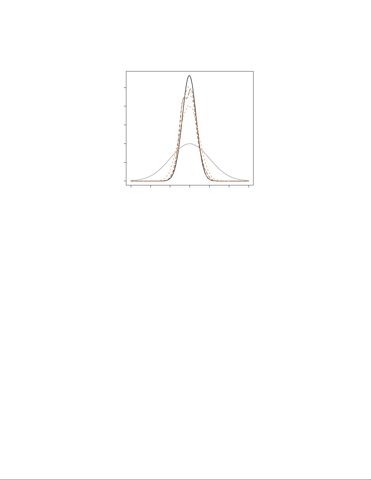
Pr oceedings of the 2011 W inter Simulation Confer ence S. J ain, R. R. Cr easey , J . Himmelspach, K. P . White, and M. Fu, eds. SIMULA TION IN ST A TISTICS Christian P . Robert Uni versit ´ e Paris-Dauphine CEREMADE 75775 Paris cede x 16, France ABSTRA CT Simulation has become a standard tool in statistics because it may be the only tool av ailable for analysing some classes of probabilistic models. W e re view in this paper simulation tools that hav e been specifically deri ved to address statistical challenges and, in particular , recent adv ances in the areas of adapti ve Mark ov chain Monte Carlo (MCMC) algorithms, and approximate Bayesian calculation (ABC) algorithms. K eywords: Monte Carlo, MCMC, ABC, SMC, importance sampling, bootstrap, maximum likelihood, Bayesian statistics, posterior distributions, Bayes factor , model choice, adapti vity , Marko v chains. 1 INTR ODUCTION Why are statistics and simulation methods so naturally intertwined? Statistics being based upon probabilistic structures, stochastic simulation appears as a natural tool to handle complex issues related to those structures, besides appealing to the statistician’ s intuition. The emergence of the subfields of computational statistics (Gentle 2009, Gentle, H ¨ ardle, and Mori 2011) is strongly related to the rise in the use of Monte Carlo methods and the history of statistics in the past 30 years exhibited a series of major advances deeply connected with simulation, whose description is the purpose of this tutorial. The cov erage is necessarily limited and the interested reader is referred to the above references and to Robert and Casella (2004) for books on simulation in statistics. 2 MONTE CARLO METHODS IN ST A TISTICS 2.1 History Simulation has appeared at the v ery early stages of the dev elopment of statistics as a field. Even though it is dif ficult to find a connection between Pierre-Simon de Laplace or Carl Gauß and simulation or between Charles Babbage or Ada Byron and statistics, the great Francis Galton devised mechanical de vices to compute estimators and distributions by means of simulation. Not only his well-known quincunx (as discussed in Stigler 1986) is a deri vation of the CL T for Bernoulli experiments, but Stigler (1997) shows that Galton also found a way to simulat e from posterior distributions by an ingenious 3D construct. Closer to Christian P . Robert us, the randomised experiments of Ronald Fisher (Fisher 1935) and the bootstrap re volution started by Brad Efron (cov ered belo w) are intrinsically connected with calculator and computer simulations, respectiv ely . While Monte Carlo methods extend much further than the field of Statistics and while giants outside our field greatly contributed to those methods (see, e.g., Halton 1970), some specific computational methods hav e been dev eloped by and for statisticians, bootstrap being the ultimate illustration. 2.2 Statistical Methods Since the primary goal of statistics is to handle data, this field is difficult to en vision without the use of numerical methods at one le vel or another . The gro wing complexification of data, models, and techniques, means that those numerical methods are becoming more and more central to the field, and that simulation methods are in particular more and more a requirement for standard statistical analyses. Here are a few examples, further illustrations being provided by Robert and Casella (2004) and Gentle (2009). The bootstrap w as introduced by Efron (1979) as a way of conducting inference for complex distrib utions or for comple x procedures without ha ving to deri ve the distribution of interest in closed form. Its appeal for this tutorial is that it simply cannot be implemented computer simulation. The idea at the core of bootstrap is that, gi ven a sample ( x 1 , . . . , x n ) , the empirical cdf b F ( x ) = n ∑ i = 1 1 n I x i ≤ x (where I A is the indicator function for the e vent A ) is a con ver ging approximation of the true cdf of the sample. Therefore, if the distribution of a procedure δ ( x 1 , . . . , x n ) is of interest, an approximation to this distribution can be obtained by assuming ( x 1 , . . . , x n ) is an iid sample from b F . Since the support of b F n is gro wing as n n , exact computations are impossible and simulation is required. The simulation requirement is very lo w since producing a bootstrap sample ( x ∗ 1 , . . . , x ∗ n ) means drawing n times with replacement from the original sample. Creating a sample of δ ( x ∗ 1 , . . . , x ∗ n ) ’ s is thus straightforward and the method can be used in an introductory course to statistics. (The theory behind is much harder , see Hall 1992.) Maximum likelihood estimation is the default estimation method in parametric settings, i.e. in cases when the data is assumed to be generated from a parameterised family of distributions, represented by a density function f ( x 1 , . . . , x n | θ ) , where θ is the parameter . It consists in selecting the v alue of the parameter that maximises the function of θ , f ( x 1 , . . . , x n | θ ) , then called the likelihood (to distinguish it from the density , a function of ( x 1 , . . . , x n ) .) Except for the most regular cases, the deriv ation of the maximum likelihood estimator is a troublesome process, either because the function is not regular enough or because it is not av ailable in closed form. An illustration of the former is a mixture model (Fr ¨ uhwirth-Schnatter 2006, Mengersen, Robert, and T itterington 2011) f ( x 1 , . . . , x n | θ ) = n ∏ i = 1 { pg ( x | µ 1 ) + ( 1 − p ) g ( x | µ 2 ) } , θ = ( p , µ 1 , µ 2 ) , where g ( ·| µ ) defines a family of probability densities and 0 ≤ p ≤ 1. This structure is usually multimodal and numerical algorithms hav e trouble handling the multimodality . An illustration of the later is a stochastic volatility model ( t = 1 , . . . , T ) x t = e z t ε t , z t = µ + ρ z t − 1 + σ η t , ε t , η t ∼ N ( 0 , 1 ) , θ = ( µ , ρ , σ ) , where only the x t ’ s are observed. In this case, the likelihood f ( x 1 , . . . , x T | θ ) ∝ Z R T + 1 T ∏ t = 1 σ − T − 1 exp  − ( z t − µ − ρ z t − 1 ) 2 / 2 σ 2  exp  − x 2 t e − 2 z t / 2 − z t  exp  − z 2 0 / 2 σ 2  d z Christian P . Robert is clearly unav ailable in closed form. Furthermore, due to the large dimension of the missing vector z , (non-Monte Carlo) numerical integration is impossible. While this specific model has emerged from the analysis of financial data, it is a special occurrence of the family of hidden Markov models where similar computational dif ficulties strike (Capp ´ e, Moulines, and Ryd ´ en 2004). Bayesian statistics are based on the same assumptions as the abov e likelihood approach, the difference being that the parameter θ is turned into an unobserved random variable for processing reasons, since it then enjoys a full probability distribution called the posterior distribution. (See Berger 1985, Bernardo and Smith 1994, or Robert 2001 for a deeper motiv ation for this approach, called Bayesian because it is based on the Bayes theorem.) Inference on the parameter θ depending on this posterior distribution, π ( θ | x 1 , . . . , x n ) , it is then ev en more natural to resort to simulation for producing estimates like posterior expectations, and ev en more for assessing the precision of the corresponding estimators. For instance, the computation of the Bayes factor used for Bayesian model comparison, B 12 ( x 1 , . . . , x n ) = R f 1 ( x 1 , . . . , x n | θ 1 ) π ( θ 1 ) d θ 1 R f 2 ( x 1 , . . . , x n | θ 1 ) π ( θ 2 ) d θ 2 , where f 1 ( x 1 , . . . , x n | θ 1 ) π ( θ 1 ) and f 2 ( x 1 , . . . , x n | θ 1 ) π ( θ 1 ) correspond to two families of distributions to be compared, is most often impossible without a simulation step (Chen, Shao, and Ibrahim 2000). Example 1 In a generalised linear model (McCullagh and Nelder 1989), a conditional distribution of y ∈ R gi ven x ∈ R p is defined via a density from an exponential family y | x ∼ exp { y · θ ( x ) − ψ ( θ ( x )) } whose natural parameter θ ( x ) depends on the conditioning variable x , θ ( x ) = g ( β T x ) , β ∈ R p that is, linearly modulo the transform g . Obviously , in practical applications like econometrics, p can be quite lar ge. Inference on β (which is the true parameter of the model) proceeds through the posterior distribution (where x = ( x 1 , . . . , x T ) and y = ( y 1 , . . . , y T ) ) π ( β | x , y ) ∝ T ∏ t = 1 exp { y t · θ ( x t ) − ψ ( θ ( x t )) } π ( β ) = exp ( T ∑ t = 1 y t · θ ( x t ) − T ∑ t = 1 ψ ( θ ( x t )) ) π ( β ) , which rarely is av ailable in closed form. In addition, in some cases ψ may be costly simply to compute and in others T may be large or ev en very large. A standard testing situation is to decide whether or not a factor , x 1 say , is influential on the dependent v ariable y . This is often translated as testing whether or not the corresponding component of β , β 1 , is equal to 0, i.e. β 1 = 0. If we denote by β − 1 the other components of β , the Bayes factor for this hypothesis will be Z R p exp ( T ∑ t = 1 y t · g ( β T x t ) − T ∑ t = 1 ψ ( g ( β T x t )) ) π ( β ) d β  Z R p − 1 exp ( T ∑ t = 1 y t · g ( β T − 1 ( x t ) − 1 ) − T ∑ t = 1 ψ ( β T − 1 ( x t ) − 1 ) ) π − 1 ( β − 1 ) d β − 1 , when π − 1 is the prior constructed for the null hypothesis. Obviously , except for the normal conjugate case, both integrals cannot be computed in a closed form. J Christian P . Robert 2.3 Monte Carlo Solutions As noted above, the setting is ripe for a direct application of simulation techniques, as the underlying probabilistic structure can exploited by either simulating pseudo-data—see, e.g., the bootstrap and the maximum likelihood approaches—or parameter v alues—for the Bayesian approach—. The use of simulation in statistics can be traced to the origins of the Monte Carlo method and simulation-based e valuations of the po wer of testing procedures are av ailable from the mid 1950’ s (Hammersley and Handscomb 1964). It is thus no surprise that the standard Monte Carlo approximation to integrals I = Z h ( x ) f ( x ) d x ≈ 1 T T ∑ t = 1 h ( x i ) , x 1 , . . . , x T ∼ f ( x ) , and the importance sampling substitutes I ≈ 1 T T ∑ t = 1 f ( x ) g ( x ) h ( x i ) , x 1 , . . . , x T ∼ g ( x ) , are thus in use in all settings where the density f ( · ) can be easily simulated, or where a good enough substitute density g ( · ) can instead be simulated (Hammersley and Handscomb 1964, Rubinstein 1981, Ripley 1987). W e recall that, because I can be represented in an infinity of ways as an expectation, there is no need to simulate from the distribution with density f to get a good approximation of I . For any probability density g with supp ( g ) including the support of h f , the integral I can also be represented as an expectation against g as above. This Monte Carlo method with importance function g almost surely con ver ges to I and the estimator is unbiased. This is classical Monte Carlo methodology (Halton 1970), ho wever the selection of importance sampling densities g ( · ) , the control of con vergence properties, the improv ement of v ariance performances were particularly studied in the 1980’ s (Smith 1984, Ge weke 1988). More advanced simulation techniques were howe ver necessary to deal with large dimensions, multimodal targets, intractable likelihoods, or/and missing data issues. Those were mostly introduced in the 1980’ s and 1990’ s, e ven though precursors can be found in earlier years (Robert and Casella 2010), and they unsurprisingly stem from the fringe of statistics (image analysis, signal processing, point processes, econometrics, surveys, etc.) where the need for more po werful computational tools was more urgent. The most important advance is undoubtedly the introduction of Markov chain Monte Carlo (MCMC) methods into statistics as it impacted the whole practice and perception of Bayesian statistics (Robert and Casella 2010). W e describe those methods in the next section. More recently , a ne w branch of computational methods called ABC (for approximate Bayesian computations) was launched by population geneticists to ov ercome computational stopping blocks due to intractable likelihoods, as described in Section 4. 3 MCMC ALGORITHMS 3.1 Mark ov Chain Monte Carlo methods As old as the Monte Carlo method itself (see Robert and Casella 2010), the MCMC e xtensions try to ov ercome the limitation of regular Monte Carlo methods (primarily , complexity or dimension of the tar get) by simulating a Markov chain whose stationary and limiting distribution is the target distribution. There exist rather generic ways of producing such chains, including Metropolis–Hastings and Gibbs algorithms. Besides the fact that stationarity of the target distribution is enough to justify a simulation method by Markov chain generation, the idea at the core of MCMC algorithms is that local exploration, when properly weighted, can lead to a valid representation of the distribution of interest, as for instance, the Metropolis–Hastings algorithm (Metropolis, Rosenbluth, Rosenbluth, T eller , and T eller 1953, Hastings 1970). Gi ven an almost arbitrary transition distribution with density q ( x , x 0 ) , the Markov chain is associated with the following transition. At time t , gi ven the current value x t , the corresponding Marko v chain explores Christian P . Robert Figure 1: Occurrences of “posterior distribution” in Google English corpus using Ngram viewer . the surface of the tar get density in the neighbourhood of x t by proposing x ∗ t + 1 ∼ q ( x t , · ) and then accepting this ne w value with probability f ( x ∗ t + 1 ) q ( x ∗ t + 1 , x t ) f ( x t ) q ( x t , x ∗ t + 1 ) ∧ 1 . The v alidation of this simple strate gy is gi ven by the detailed balance property of the Metropolis–Hastings transition density , µ ( x , x 0 ) , namely that f ( x ) µ ( x , x 0 ) = f ( x 0 ) µ ( x 0 , x ) . This MCMC simulation technique is obviously generic and thus applies in many other fields than statistics, b ut the reassessment of the method in the 1980’ s by sev eral statisticians (including Julian Besag, Don and Stuart Geman, Brian Ripley , David Spiegelhalter , Martin T anner , Alan Gelfand and Adrian Smith, as detailed in Robert and Casella 2010) brought a considerable impetus to the development of Bayesian statistical methodology by providing a general way of handling high dimensional problems and complex densities. An illustration of this surge is produced in Figure 1 which shows how the use of the term “posterior distribution” considerably increased after 1990, following Gelfand and Smith (1990) who advertised the Gibbs sampler as a mean of exploring posterior distributions. The difficulty inherent to Metropolis–Hastings algorithms like the random w alk version, where q ( x , x 0 ) is symmetric, is the scaling of the proposal distrib ution: the scale of q must correspond to the shape of the target distribution so that, in a reasonable number of steps, the whole support of this distrib ution can be visited. If the scale of the proposal is too small, this will not happen as the algorithm stays “too local” and, if there are several modes on the target, the algorithm may get trapped within one modal region because it cannot reach other modal regions relying on jumps of too small a magnitude. The larger the dimension p of the target is, the harder it is to set up an efficient proposal, because (a). the curse of dimension implies that there is a lar ger portion of the space with zero probability; (b). the knowledge and intuition about the modal regions get weaker; (c). the scaling parameter is a symmetric ( p , p ) matrix Ξ in the proposal q ( x , x 0 ) = g (( x − x 0 ) T Ξ ( x − x 0 )) . Even when the matrix Ξ is diagonal, it gets harder to chose as the dimension increases. Unfortunately , an on-line scaling of the algorithm by looking for instance at the empirical acceptance rate is theoretically flawed in that it cancels the Marko v v alidation. Furthermore, the attraction of a modal region may give a false sense of con vergence and lead to a choice of too small a scale, simply because other modes will not be visited during the scaling experiment. 3.2 The Challenge of Adaptivity Thus, giv en the range of situations where MCMC applies, it is unrealistic to hope for a generic MCMC sampler that would function in ev ery possible setting. The reason for this “impossibility theorem” is that, in genuine problems, the complexity of the distrib ution to simulate is the very reason why MCMC is used! So it is unrealistic to ask for a prior opinion about this distribution, its support, or the parameters of the proposal distribution used in the MCMC algorithm: intuition is close to null in most of these problems. Christian P . Robert Ho wever , the performances of off-the-shelf algorithms like the random-walk Metropolis–Hastings scheme bring information about the distrib ution of interest or at least about the adequacy of the current proposal and, as such, could be incorporated in the design of more efficient algorithms. The difficulty is that one usually miss the time to train the algorithm on these pre vious performances. While it is natural to think that the information brought by the first steps of an MCMC algorithm should be used in later steps, the v alidation of such a learning mechanism is complex, because of its non-Markovian nature. Usual ergodic theorems do not apply in such cases. Further , it may be that, in practice, such algorithms do degenerate to point masses due to too a rapid decrease in the v ariability of their proposal. Example 2 Consider a t -distribution T ( ν , θ , 1 ) sample ( x 1 , . . . , x n ) with ν known. Assume in addition a flat prior π ( θ ) = 1. While the posterior distrib ution on θ can be easily plotted, up to a normalising constant, direct simulation and computation from this posterior is impossible. In an MCMC frame work, we could fit a normal proposal from the empirical mean and v ariance of the previous values of the chain, µ t = 1 t t ∑ i = 1 θ ( i ) and σ 2 t = 1 t t ∑ i = 1 ( θ ( i ) − µ t ) 2 . This leads to a Metropolis–Hastings algorithm with acceptance probability n ∏ j = 2 " ν + ( x j − θ ( t ) ) 2 ν + ( x j − ξ ) 2 # − ( ν + 1 ) / 2 exp − ( µ t − θ ( t ) ) 2 / 2 σ 2 t exp − ( µ t − ξ ) 2 / 2 σ 2 t , where ξ is generated from N ( µ t , σ 2 t ) . The in validity of this scheme (related to the dependence on the whole past values of θ ( i ) ) is illustrated by Figure 2: for an initial variance of 2 . 5, there is a bias in the fit, e ven after stabilisation of the empirical mean and v ariance. J Figure 2: Comparison of the distrib ution of an adapti ve scheme sample of 25 , 000 points with initial v ariance of 2 . 5 and of the target distribution. The overall message is thus that one should not constantly adapt the proposal distribution on the past performances of the simulated chain. Either the adaptation must cease after a period of burnin (not to be taken into account for the computations of expectations and quantities related to the target distribution), or the adapti ve scheme must be theoretically assessed on its o wn right. If we remain within the MCMC approach (rather than adopting sequential importance methods as in Capp ´ e, Douc, Guillin, Marin, and Robert 2008), this later path is not easy and only a small community (gathering at the Adap’ ski workshops, run ev ery three year since 2005) is working on establishing valid adapti ve schemes. Earlier works include those of Gilks, Roberts, and Sahu (1998) who use regeneration to create block independence and preserve Markovianity on the paths rather than on the v alues, Haario, Saksman, and T amminen (1999), Haario, Saksman, and T amminen (2001) who deri ve a proper adaptation scheme in the spirit of stochastic optimisation by using a ridge-like correction to the empirical v ariance, and Andrieu and Robert (2001) who propose a more general frame work of v alid adaptivity based on stochastic optimisation and the Robbin-Monro algorithm. Christian P . Robert The latter actually embeds the chain of interest θ ( t ) in a larger chain ( θ ( t ) , ξ ( t ) , ∂ ( t ) ) that also includes the parameter of the proposal distrib ution as well as the gradient of a performance criterion. More recent works building on this principle and deriving sufficient conditions for ergodicity include Andrieu and Moulines (2006), Roberts and Rosenthal (2007), Craiu, Rosenthal, and Y ang (2009), Saksman and V ihola (2010), Atchad ´ e (2011), Atchad ´ e and Fort (2010), Ji and Schmidler (2011). They mostly contain dev elopment of a theoretical nature. This line of research has led Roberts and Rosenthal (2009) to establish guiding rules as to when an adapti ve MCMC algorithm is con verging to the correct tar get distribution, to the point of constructing an R package called amcmc (Rosenthal 2007). More precisely , Roberts and Rosenthal (2009) propose a diminishing adaptation condition that states that the total v ariation distance between two consecutiv e kernels must uniformly decrease to zero (which does not mean that the kernel must con verge!). For instance, a random walk proposal that relies on the empirical variance of the sample will satisfy this condition. The scale of the random walk is then tuned in each direction to ward an optimal acceptance rate of 0 . 44. T o this ef fect, for each component of the simulated v ector , a factor δ i corresponding to the logarithm of the random walk standard deviation is updated ev ery 50 iterations by adding or subtracting a factor ε t depending on whether or not the average acceptance rate on that batch of 50 iterations and for this component was above or belo w 0 . 44. If ε t decreases to zero as min ( . 01 , 1 / √ t ) , the conditions for conv ergence are satisfied. Another package called Grapham was also recently dev eloped by V ihola (2010). 4 ABC METHODS 4.1 Intractable Likelihoods When facing settings where the likelihood ` ( θ | y ) is not av ailable in closed form, the abov e solutions are not directly av ailable. In the particular set-up of hierarchical models with partly conjugate priors, it may be that the corresponding conditional distributions can be simulated and this property leads to a Gibbs sampler Gelfand and Smith (1990), but such a decomposition is not av ailable in general. In the specific setting of latent v ariable models, the likelihood may be expressed as an intractable multidimensional integral ` ( θ | y ) = Z ` ? ( θ | y , u ) d u , where y is observed and u ∈ R p is not, while the joint distribution π ( θ , z | y ) ∝ π ( θ ) ` ? ( θ | y , u ) can be simulated. The increase in dimension induced by the passage from θ to ( θ , u ) may be such that the con ver gence properties of the corresponding MCMC algorithms are too poor for the algorithm to be considered. Bayesian inference thus needs to handle a large class of settings where the likelihood function is not completely kno wn, and where exact (or even MCMC) simulation from the corresponding posterior distribution is impractical or e ven impossible. The ABC methodology , where ABC stands for appr oximate Bayesian computation , of fers an almost automated resolution of the difficulty with intractable-yet-simulable models. It was first proposed in population genetics by T av ar ´ e, Balding, Grif fith, and Donnelly (1997) who bypassed the computation of the likelihood function using simulation. Pritchard, Seielstad, Perez-Lezaun, and Feldman (1999) then produced a generalisation based on an approximation of the tar get. 4.2 A pproximati ve Resolution The principle of the ABC algorithm (T av ar ´ e, Balding, Grif fith, and Donnelly 1997) is a simple accept-reject algorithm: if one k eeps simulating θ ∼ π ( θ ) and x ∼ f ( x | θ ) until x = y , the resulting θ is distrib uted from π ( θ | y ) ∝ π ( θ ) f ( y | θ ) . Howe ver , when the ev ent x = y has probability zero, the algorithm cannot be implemented. Pritchard, Seielstad, Perez-Lezaun, and Feldman (1999) used instead an approximation of the abov e by simulating pairs ( θ ) , x until the condition ρ { η ( z ) , η ( y ) } ≤ ε Christian P . Robert −3 −2 −1 0 1 2 3 0.0 0.2 0.4 0.6 0.8 1.0 x Figure 3: Approximations of the genuine posterior distrib ution (in dark) by ABC versions for ε equal to the . 01 , . 1 , 1 , 10 % quantiles of 10 6 sampled distances. The prior distribution is the gr ey curve. is met, where η is a (maybe insufficient) statistic, ρ is a distance, and ε > 0 is a tolerance lev el. The abov e algorithm is “likelihood-free” in that it only requires the ability to simulate from the distribution f ( x | θ ) and it is approximative in that it produces simulations from π ε ( θ | y ) = Z Z π ( θ ) f ( z | θ ) I A ε , y ( z ) d z . Z A ε , y × R d π ( θ ) f ( z | θ ) d z d θ , (1) where I B ( · ) denotes the indicator function of the set B and where A ε , y = { z ∈ D | ρ { η ( z ) , η ( y ) } ≤ ε } . The basic idea behind ABC is that using a representative (enough) summary statistic η coupled with a small (enough) tolerance ε should produce a good (enough) approximation to the posterior distribution. At a deeper le vel, the algorithm implements a non-parametric approximation of the conditional distrib ution using binary kernels (Beaumont, Zhang, and Balding 2002, Blum 2010, Blum and Franc ¸ ois 2010). Example 3 Considering the toy problem of Example 2, a simple implementation of the ABC algorithm consists in simulating the location parameter θ from the prior —chosen to be a N ( 0 , 1 ) — and in simulating n realisations from a T ( ν , θ , 1 ) distribution until those n realisations are close enough from the original observ ations. In generic ABC algorithms, the tolerance ε is chosen as a quantile of the distances between the true data and the simulated pseudo-data. Figure 3 studies the impact of this choice starting from the 10% quantile do wn to the . 01% quantile. The ABC approximations get closer to the true posterior as ε decreases, the final approximation dif fering more for variance than for bias reasons. J In more realistic problems, simulating from the prior distribution is very inefficient because it does not account for the data at the proposal stage and thus leads to proposed values located in low posterior probability regions. As an answer to this problem, Marjoram, Molitor , Plagnol, and T av ar ´ e (2003) hav e introduced an MCMC-ABC algorithm targeting (1). Sequential alternativ es can also enhance the ef ficiency Christian P . Robert of the ABC algorithm, by learning about the target distribution, as in the ABC-PMC algorithm—based on genuine importance sampling arguments—of Beaumont, Cornuet, Marin, and Robert (2009) and the ABC-SMC algorithm—deriving a sequential Monte Carlo (SMC) filter—of Del Moral, Doucet, and Jasra (2011) and Drov andi and Pettitt (2010). 4.3 Con vergence and Limitations While the original argument of letting ε go to zero is clearly illustrated by the above example, more adv anced arguments have been recently produced about the con ver gence of ABC algorithms. Besides the non-parametric parallels dra wn in Beaumont, Zhang, and Balding (2002), Blum (2010), Blum and Franc ¸ ois (2010), a different perspectiv e is found in the pseudo-likelihoods argument of Fearnhead and Prangle (2010) and Dean, Singh, Jasra, and Peters (2011). In this perspectiv e, ABC is an exact algorithm for an approximate distribution, which is con verging to the exact posterior as the sample size grows to infinity . ABC being able to produce samples from posterior distributions, it does not come as a surprise that it is used for model choice because the latter often in volv es a computational complexification. Estimating the posterior probabilities of models under competition by ABC is thus proposed in most of the literature (see, e.g., Cornuet, Santos, Beaumont, Robert, Marin, Balding, Guillemaud, and Estoup 2008, Grelaud, Marin, Robert, Rodolphe, and T ally 2009, T oni, W elch, Strelko wa, Ipsen, and Stumpf 2009, T oni and Stumpf 2010). Howe ver , it has been recently exposed in Didelot, Everitt, Johansen, and Lawson (2011), Robert, Cornuet, Marin, and Pillai (2011) that those approximations may fail to con ver ge in the case the summary statistics are not sufficient for model comparison. More empirical ev aluations as those tested in Ratmann, Andrieu, Wiujf, and Richardson (2009) should thus be implemented to assess the rele vance of those approximations, unless one uses the whole data instead of summary statistics. 5 CONCLUSION The present tutorial is naturally both very incomplete and quite partial. Even within Bayesian methods, one glaring omission is the area of sequential Monte Carlo methods (or particle filters) used to analyse non-linear non-Gaussian state space models. While particle filters and impro vements have been around for se veral years (Gordon, Salmond, and Smith 1993, Pitt and Shephard 1999, Del Moral, Doucet, and Jasra 2006), handling unknown parameters as well is a much harder goal and it is only recently that significant progress has been made with the particle MCMC method of Andrieu, Doucet, and Holenstein (2011). This new class of MCMC algorithms relies on a population of particles produced by an SMC algorithm to build an efficient proposal at each MCMC iteration. (That this approximation remains a valid MCMC algorithm is quite an inv olved resul, in connection with the results of Andrieu and Roberts 2009). This area is currently quite acti ve with alternativ es and softwares being de veloped. More generally , parallel computing is now used in a gro wing fraction of applications, particularly in genetics, with a direct impact on the nature of the simulation methods (T om, Sinsheimer , and Suchard 2010, Jacob, Robert, and Smith 2011), which include more and more non-parametric aspects (Jordan 2010, Hjort, Holmes, M ¨ uller , and W alker 2010). Simulation techniques are clearly found in too many of current statistical methods to be e ven mentioned here and the trend is definitely upward. Speed (2011) concludes “we are heading to an era when all statistical analysis can be done by simulation”. This is indeed quite an exciting time for computational statisticians! A CKNO WLEDGEMENTS This research is supported partly by the Agence Nationale de la Recherche through the 2009-2012 grants Big MC and EMILE and partly by the Institut Uni versitaire de France (IUF). Christian P . Robert REFERENCES Andrieu, C., A. Doucet, and R. Holenstein. 2011. “Particle Markov chain Monte Carlo (with discussion)”. J . Royal Statist. Society Series B 72 (2):269–342. Andrieu, C., and ´ E. Moulines. 2006. “On the ergodicity properties of some adapti ve MCMC algorithms”. Ann. Applied Pr obability 16 (3): 1462–1505. Andrieu, C., and C. Robert. 2001. “Controlled Marko v chain Monte Carlo methods for optimal sampling”. T echnical Report 0125, Uni versit ´ e Paris Dauphine. Andrieu, C., and G. Roberts. 2009. “The pseudo-mar ginal approach for efficient Monte Carlo computations”. Ann. Statist. 37 (2): 697–725. Atchad ´ e, Y . 2011. “K ernel estimators of asymptotic v ariance for adaptiv e Markov Chain Monte Carlo”. Ann. Statist. 39 (2): 990–1011. Atchad ´ e, Y ., and G. Fort. 2010. “Limit theorems for some adaptiv e MCMC algorithms with subgeometric kernels”. Bernoulli 16(1):116–154. Beaumont, M., J.-M. Cornuet, J.-M. Marin, and C. Robert. 2009. “ Adaptiv e approximate Bayesian Com- putation”. Biometrika 96(4):983–990. Beaumont, M., W . Zhang, and D. Balding. 2002. “ Approximate Bayesian Computation in Population Genetics”. Genetics 162:2025–2035. Berger , J. 1985. Statistical Decision Theory and Bayesian Analysis . Second ed. Springer-V erlag, New Y ork. Bernardo, J., and A. Smith. 1994. Bayesian Theory . Ne w Y ork: John W iley . Blum, M. 2010. “Approximate Bayesian Computation: a non-parametric perspectiv e”. J . American Statist. Assoc. 105 (491): 1178–1187. Blum, M., and O. Franc ¸ ois. 2010. “Non-linear re gression models for Approximate Bayesian Computation”. Statist. Comput. 20:63–73. Capp ´ e, O., R. Douc, A. Guillin, J.-M. Marin, and C. Robert. 2008. “ Adaptiv e importance sampling in general mixture classes”. Statist. Comput. 18:447–459. Capp ´ e, O., E. Moulines, and T . Ryd ´ en. 2004. Hidden Markov Models . Springer-V erlag, New Y ork. Chen, M., Q. Shao, and J. Ibrahim. 2000. Monte Carlo Methods in Bayesian Computation . Springer -V erlag, Ne w Y ork. Cornuet, J.-M., F . Santos, M. Beaumont, C. Robert, J.-M. Marin, D. Balding, T . Guillemaud, and A. Estoup. 2008. “Inferring population history with DIY ABC: a user-friendly approach to Approximate Bayesian Computation”. Bioinformatics 24 (23): 2713–2719. Craiu, R., J. Rosenthal, and C. Y ang. 2009. “Learn from thy neighbour: Parallel-chain and re gional adapti ve MCMC”. J . American Statist. Assoc. 104 (488): 1454–1466. Dean, T . A., S. S. Singh, A. Jasra, and G. W . Peters. 2011. “Parameter Estimation for Hidden Markov Models with Intractable Likelihoods”. T echnical Report arXiv:1103.5399, Cambridge Uni versity Engineering Department. Del Moral, P ., A. Doucet, and A. Jasra. 2006, June. “Sequential Monte Carlo samplers”. J. Royal Statist. Society Series B 68 (3): 411–436. Del Moral, P ., A. Doucet, and A. Jasra. 2011. “An adapti ve sequential Monte Carlo method for approximate Bayesian computation”. Bernoulli . (T o appear .). Didelot, X., R. Everitt, A. Johansen, and D. La wson. 2011. “Likelihood-free estimation of model evidence”. Bayesian Analysis 6:48–76. Drov andi, C., and A. Pettitt. 2010. “Estimation of Parameters for Macroparasite Population Evolution Using Approximate Bayesian Computation”. Biometrics . (T o appear .). Efron, B. 1979. “Bootstrap methods: another look at the jacknife”. Ann. Statist. 7:1–26. Fearnhead, P . and Prangle, D. 2010. “Semi-automatic Approximate Bayesian Computation”. Arxi v preprint arXi v . Fisher , R. 1935. The Design of Experiments. Oliv er & Boyd. Christian P . Robert Fr ¨ uhwirth-Schnatter , S. 2006. F inite Mixtur e and Markov Switching Models . Ne w Y ork: Springer-V erlag, Ne w Y ork. Gelfand, A., and A. Smith. 1990. “Sampling based approaches to calculating mar ginal densities”. J. American Statist. Assoc. 85:398–409. Gentle, J., W . H ¨ ardle, and Y . Mori. 2011. Handbook of Computational Statistics—Concepts and Methods . Second ed. Berlin: Springer-V erlag. Gentle, J. E. 2009. Computational Statistics. Ne w Y ork: Springer–V erlag. Ge weke, J. 1988. “ Antithetic acceleration of Monte Carlo integration in Bayesian inference”. J. Economet- rics 38:73–90. Gilks, W ., G. Roberts, and S. Sahu. 1998. “ Adaptiv e Markov Chain Monte Carlo”. J. American Statist. Assoc. 93:1045–1054. Gordon, N., J. Salmond, and A. Smith. 1993. “ A nov el approach to non-linear/non-Gaussian Bayesian state estimation”. IEEE Pr oceedings on Radar and Signal Pr ocessing 140:107–113. Grelaud, A., J.-M. Marin, C. Robert, F . Rodolphe, and F . T ally . 2009. “Likelihood-free methods for model choice in Gibbs random fields”. Bayesian Analysis 3(2):427–442. Haario, H., E. Saksman, and J. T amminen. 1999. “ Adapti ve Proposal Distrib ution for Random W alk Metropolis Algorithm”. Computational Statistics 14(3):375–395. Haario, H., E. Saksman, and J. T amminen. 2001. “ An Adaptive Metropolis Algorithm”. Bernoulli 7 (2): 223–242. Hall, P . 1992. The Bootstrap and Edgeworth Expansion . Springer-V erlag, New Y ork. Halton, J. 1970. “A retrospective and prospectiv e surv ey of the Monte Carlo method”. Siam Review 12 (1): 1–63. Hammersley , J., and D. Handscomb . 1964. Monte Carlo Methods . New Y ork: John W iley . Hastings, W . 1970. “Monte Carlo sampling methods using Markov chains and their application”. Biometrika 57:97–109. Hjort, N., C. Holmes, P . M ¨ uller , and S. W alker . 2010. Bayesian nonparametrics . Cambridge Univ ersity Press. Jacob, P ., C. Robert, and M. Smith. 2011. “Using parallel computation to impro ve independent Metropolis– Hastings based estimation”. J . Comput. Graph. Statist. . (T o appear .). Ji, C., and S. Schmidler . 2011. “ Adapti ve Marko v chain Monte Carlo for Bayesian V ariable Selection”. J. Comput. Graph. Statist. . (T o appear). Jordan, M. 2010. Bayesian nonparametric learning: Expressive priors for intelligent systems . College Publications. Marjoram, P ., J. Molitor , V . Plagnol, and S. T av ar ´ e. 2003, December . “Marko v chain Monte Carlo without likelihoods”. Pr oc. Natl. Acad. Sci. USA 100 (26): 15324–15328. McCullagh, P ., and J. Nelder . 1989. Generalized Linear Models . Chapman and Hall, New Y ork. Mengersen, K., C. Robert, and D. T itterington. 2011. Mixtur es: Estimation and Applications . John Wile y . Metropolis, N., A. Rosenbluth, M. Rosenbluth, A. T eller, and E. T eller . 1953. “Equations of state calculations by fast computing machines”. J. Chem. Phys. 21 (6): 1087–1092. Pitt, M., and N. Shephard. 1999. “Filtering via simulation: auxiliary particle filters”. J. American Statist. Assoc. 94 (446): 590–599. Pritchard, J., M. Seielstad, A. Perez-Lezaun, and M. Feldman. 1999. “Population growth of human Y chromosomes: a study of Y chromosome microsatellites”. Mol. Biol. Evol. 16:1791–1798. Ratmann, O., C. Andrieu, C. W iujf, and S. Richardson. 2009. “Model criticism based on likelihood-free inference, with an application to protein network ev olution”. Pr oc. Natl. Acad. Sciences USA 106:1–6. Ripley , B. 1987. Stochastic Simulation . Ne w Y ork: John W iley . Robert, C. 2001. The Bayesian Choice . second ed. Springer -V erlag, New Y ork. Robert, C., and G. Casella. 2004. Monte Carlo Statistical Methods . second ed. Springer -V erlag, New Y ork. Christian P . Robert Robert, C., and G. Casella. 2010. “ A history of Marko v Chain Monte Carlo-Subjectiv e recollections from incomplete data”. In Handbook of Markov Chain Monte Carlo: Methods and Applications , Edited by S. Brooks, A. Gelman, X. Meng, and G. Jones: Chapman and Hall, Ne w Y ork. Robert, C., J.-M. Cornuet, J.-M. Marin, and N. Pillai. 2011. “Lack of confidence in ABC model choice”. T echnical Report arxi v .org:1102.4432, CEREMADE, Univ ersit ´ e Paris Dauphine. Roberts, G., and J. Rosenthal. 2007. “Coupling and er godicity of adapti ve Marko v Chain Monte carlo algorithms”. J . Applied Pr oba. 44(2):458–475. Roberts, G., and J. Rosenthal. 2009. “Examples of Adaptiv e MCMC”. J. Comp. Graph. Stat. 18:349–367. Rosenthal, J. 2007. “ AMCM: An R interface for adaptiv e MCMC”. Comput. Statist. Data Analysis 51:5467– 5470. Rubinstein, R. 1981. Simulation and the Monte Carlo Method . Ne w Y ork: John W iley . Saksman, E., and M. V ihola. 2010. “On the ergodicity of the adapti ve Metropolis algorithm on unbounded domains”. Ann. Applied Pr obability 20(6):2178–2203. Smith, A. 1984. “Present position and potential de velopments: some personal view on Bayesian statistics”. J . Royal Statist. Society Series A 147:245–259. Speed, T . 2011. “Simulation”. IMS Bulletin 40(3):18. Stigler , S. 1986. The History of Statistics . Cambridge: Belknap. Stigler , S. 1997. “Re gression tow ards the mean, historically considered”. Statistical Methods in Medical Resear ch 6 (2): 103. T av ar ´ e, S., D. Balding, R. Grif fith, and P . Donnelly . 1997. “Inferring coalescence times from DN A sequence data”. Genetics 145:505–518. T om, J., J. Sinsheimer , and M. Suchard. 2010. “Reuse, recycle, re weigh: Combating influenza through ef ficient sequential Bayesian computation for massive data”. 4 (4): 1722–1748. T oni, T ., and M. Stumpf. 2010. “Simulation-based model selection for dynamical systems in systems and population biology”. Bioinformatics 26 (1): 104–110. T oni, T ., D. W elch, N. Strelkow a, A. Ipsen, and M. Stumpf. 2009. “Approximate Bayesian computation scheme for parameter inference and model selection in dynamical systems”. Journal of the Royal Society Interface 6 (31): 187–202. V ihola, M. 2010. “Graphical models with adaptiv e random walk Metropolis algorithms”. Comput. Statist. Data Anal. 54(1):49–54. A UTHOR BIOGRAPHY CHRISTIAN P . R OBER T is Professor in the Department of Applied Mathematics at the Universit ´ e Paris- Dauphine since 2000. He is also a 2010-2015 senior member of the Institut Uni versitaire de France, and the former Head of the Statistics Laboratory of the Centre de Recherche en Economie et Statistique (CREST). He was previously Professor at the Uni versit ´ e de Rouen from 1992 till 2000 and has held visiting positions in Purdue Uni versity , Cornell Univ ersity , and the Univ ersity of Canterbury , Christchurch, Ne w-Zealand. He is currently an adjunct professor in the Department of Mathematics and Statistics at the Queensland Uni versity of T echnology (QUT), Brisbane, Australia. He is a Fellow of the Royal Statistical Society and of the Institute of Mathematical Statistics (IMS), as well as a Medallion Lecturer of the IMS. He was Editor of the Journal of the Royal Statistical Society Series B from 2006 till 2009 and has been an associate editor of the Annals of Statistics , J ournal of the American Statistical Society , Statistical Science , Sankhya . He is currently an Area Editor for the ACM T ransactions on Modeling and Computer Simulation (TOMA CS) journal. He was the 2008 President of the International Society for Bayesian Analysis (ISB A). His research areas cover Bayesian statistics, with a focus on decision theory and model selection, numerical probability , with works cantering on the application of Mark ov chain theory to simulation, and computational statistics, de veloping and ev aluating ne w methodologies for the analysis of statistical models.