Behavior of Graph Laplacians on Manifolds with Boundary

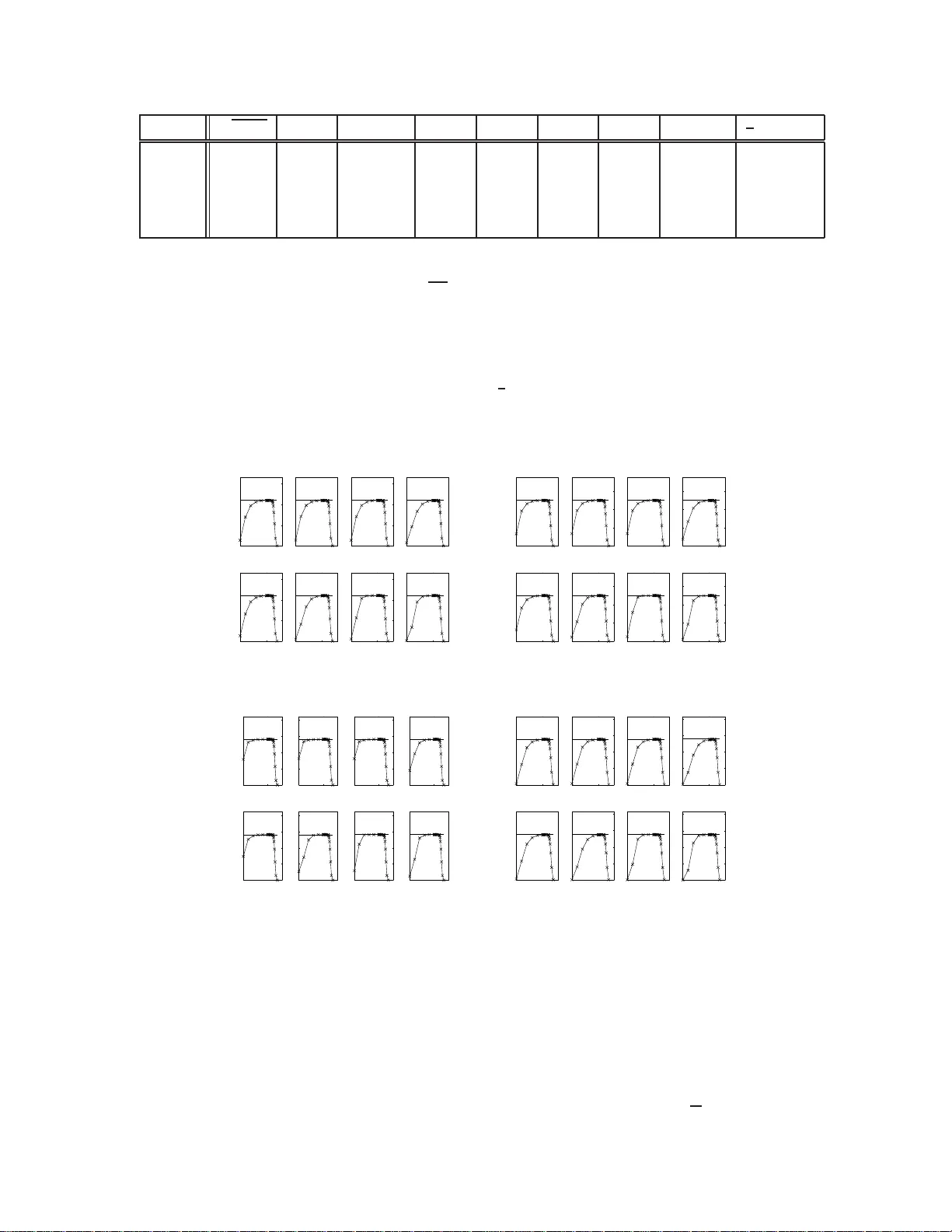
Beha vior of Graph Laplacians on Manif olds with Boundary Xueyuan Zhou Departmen t of C omp uter Science University of Chicago zhouxy@cs.uch icago.edu Mikhail Belkin Departmen t of Computer Science and Eng ineering Ohio State Uni versity mbelkin@cse.o hio-state.edu Abstract In manifold learning , algorith ms based on graph Laplacians constructed from data have recei ved considerab le attention both in practical ap plications and theor etical a nalysis. In particular, the conv ergence of grap h Laplacians obtain ed from sam pled data to certain continu ous operators has become an active researc h top ic r ecently . Most o f the existing work has been done under th e assumption that the data is sampled from a manifold withou t boundary or that the function s of interests are evaluated at a p oint away fro m the b ound ary . Howe ver , th e que stion of b ound ary behavior is o f considerab le practical and theo retical in terest. In this p aper we provide an an alysis of the behavior o f graph Laplac ians at a po int near or o n the bou ndary , d iscuss their convergence rates an d their implication s and provide some nu merical results. It turns out th at while poin ts near the boun dary o ccupy on ly a small p art of the to tal volume of a manifo ld, the behavior of graph Laplacian there has d ifferent scaling properties fr om its beh avior else where on the manifold, with global effects on the whole manifo ld, an observation with potentially important implication s for the general problem of learning on manifold s. 1 Intr oduction Graph Laplacian constructed from data points is a key elemen t in many machine learning algor ithms includ ing spectral clustering, e.g ., ( von Lux burg, 2007), semi-supervised learn ing (Zh u, 2006; Chapelle et al., 2006) and dimensiona lity reduction (Belkin & Niyogi, 200 3), as well as a number of other applications. A large amount of work in recent year s has be en c entered on an alyzing various theoretical aspec ts o f grap h Laplacians on manifold s, and , in particular, on their different modes of con vergence, when the data goes to infinity and/or the p arameters, such as kern el b andwidth, tend to zer o (Belk in, 2003 ; L afon, 200 4; Hein, 200 5; Coifm an & Laf on, 20 06; Sing er, 2006 ; Gin ´ e & K oltchinsk ii, 2006; Hein et al., 2007 ; Belkin & Niyogi, 2 008; von Luxburg et al., 2008; Rosasco et al., 201 0). A typical result in th at dir ection shows that the discrete grap h Laplacian conver ges 1 to the Lap lacian-Beltrami operato r on manifolds wh en the band width p arameter of the kern el is cho sen as an appr opriate fun ction of the numb er of data points. These results help to clarify our unde rstanding of the und erlying ob jects, to she d light on p roperties of the algo rithms and to guide the selection of algorithm s in prac tical applications. For example, an analy sis of norm alized versus u nnorm alized Laplacians in (von Luxburg et a l., 2 008)) suggests that norm alization may be pref erable in pr actical applicatio ns. In anoth er example, the estimators of sev eral graph La placian based semi-superv ised learning algorithms had recently been shown to conver ge to constant solutions in the limit of infin ite unlabeled points while fixing labeled points (Nadler et al., 200 9), suggesting the use of iterated Laplac ians (Zhou & Belkin, 2 011), which in deed shows superior per forman ce in practice. The s pectra l con vergence of a graph Laplacia n is another important limit analysis of the graph Laplacian , which lin ks d irectly to applications. The empirical sp ectral convergence o f spectr al clustering when th e sample size n goes to infinity for a fixed k ernel bandwidth t was studied by (von Luxburg et al., 2008) , while the spectral conv ergence of a graph Laplacian to the Laplace -Beltrami operator when the kernel bandwidth t goes to zero as n goes to infinity is studied in (Belkin & Niyog i, 2007). Howe ver , most previous re sults o n graph Lapla cians deal with the setting where the man ifold d oes n ot have a bou ndary o r when the operator is analyzed at a point away from the bo undar y . Arguably , it is a 1 Different modes of con verg ence are possible here, such as different types of pointwise or uniform con v ergence or con v ergence of eigen vectors. significant short-comin g of th ese analyses, since manifolds o r d omains with bo undary ar e present exp licitly or implicitly in many p roblems of significan t inter est in data an alysis. Perhaps the simplest example is the fact th at the pixel intensity of a gr ay-scale image c annot b e smaller than ze ro, providin g a natural bou ndary condition for any image manifolds. A more intere sting example is in motion analysis, where the manifo ld of configur ations of a human or rob ot b ody (perhaps em bedded using video imag es or data from sensors attach ed to limb s) ha s bou ndaries corr espondin g to the limits for the ran ge of m otions of each in dividual joint. M ore generally , it is natural to think that boundar ies in data are present whenever the generating pro cess itself is in some way constrained . It is clear that if such man ifolds are to be learn ed from data, the bo undar y behavior cannot be disregarded. In the curren t paper we discuss the boundar y behavior of graph Laplacian s by analyzing the grap h Lapla- cian conv ergence at the boundary . W e show that the gra ph Laplacian at the boundary converges to a gradient operator in the direction norm al to the bo undary , when the band width par ameter t is chosen adaptively as a function of the number of data p oints. W e provide exp licit bounds for the con vergence. One of the ke y results of our analy sis is that both the behavior and the scaling of the grap h Laplac ian near the boundary is quite dif- ferent from that in th e interior of the man ifold. Specifically , for a fixed function f ( x ) an d a small band width parameter t th e (approp riately scaled) graph Laplacian will be close to the Laplace-Beltrami oper ator ∆ f ( x ) on interior point x , while at the boundar y the same object will be close to th e normal deriv ativ e 1 √ t ∂ n f ( x ) . W e see that the large v alues of the graph Laplacian ap plied to a fixed function are likely to correspon d to th e bound ary points. Mo reover , the analysis shows that while there are few points n ear the bound ary of a m ani- fold, th eir influenc e on the gr aph Laplacian is disprop ortionately large and canno t be ignored . Th is sugg ests that the bo undar y has a global effect on the grap h Laplacian, a findin g th at is con firmed by o ur numerica l experiments provided in the pap er . V iewed in a different way it sug gests th at for alg orithms wh en a gr aph Laplacian is u sed as a regularizer, as is the case in ma ny applicatio ns, boun ding the n orm would lead to the sup pression o f th e large values near the bo undar y . Th us the minimizer of the regular ization prob lem (or similarly , the e igenv ectors) sh ould satisfy the Neumann bo undar y cond itions, i.e., be nearly con stant in the direction orthog onal to the bo undary , which is confirmed by our numerical experiments. In a related line of in vestigation we find that the symmetric normalized graph Laplacian L s has a dif ferent bound ary behavior from the rand om walk (asymmetric normalized) and unnor malized graph Laplacians. Un- like those two, for a fixed function f ( x ) , L s f ( x ) co n verges to 1 √ t [ p ( x )] 1 / 2 ∂ n ( f ( x ) / [ p ( x )] 1 / 2 ) for a bound ary point x , where p ( x ) is the pro bability density function. Th is do es not lead to th e Neu mann bou ndary cond i- tion, and seems strange from a practical point of view . As a further illustration o f the importance of boundary conditio ns in learning th eory , we explore the bound ary effects fo r a repro ducing kernel in a simple 1-d imensional example. W e also discuss th e limit of the graph Laplacian regularizer on manifold s with bou ndary , which cannot be taken fo r granted to be the same as the limit on R N or manifold s without bou ndary because of the boundary behavior of graph Laplacian s. Finally we briefly c ompare the gra ph Lap lacian built from random samp les to the L aplacian o n regular grids in numerical PDE’ s. 1.1 Problem Setting W e now proceed with a more technical setting of the pro blem. Let Ω be a comp act Riemannian submanifold of intrin sic dimension d e mbedd ed in R N , Ω the interior of Ω , and ∂ Ω the bou ndary of Ω , which we will assume to satisfy the n ecessary smoothn ess co nditions 2 . Giv en n rand om sam ples X = { X 1 , · · · , X n } drawn i.i.d. from a distribution with a smooth density function p ( x ) on Ω such th at 0 < a ≤ p ( x ) ≤ b < ∞ , we can b uild a weighted gr aph G ( V , E ) by map ping each sam ple po int X i to vertex v i and assigning a weight w ij to edge e ij . One typical weight function is the Gaussian defined as w ij = K t ( X i , X j ) = 1 /t d/ 2 e −k X i − X j k 2 R N /t , which is used in this pape r . Let the n × n matrix W be the edg e weig ht m atrix of graph G with W ( i, j ) = w ij , an d D be a diago nal matrix such th at D ii = P j w ij , the n the unn ormalized graph Laplacian is defined as matrix L u L u = D − W (1) There ar e several ways of norm alizing L u . For in stance, the most co mmon ly u sed two are the a symmetric random walk no rmalized version L r = D − 1 L u = I − D − 1 W and the symmetric no rmalized version L s = D − 1 / 2 L u D − 1 / 2 = I − D − 1 / 2 W D − 1 / 2 . Another useful way of b uildin g a grap h Laplacian is gov erned by a parameter α such that we first normal- ize W as W α = D − α W D − α , then d efine the u nnorm alized, random walk and symmetric nor malized graph 2 Instead of spending sev eral pages to describe t hese smoothness conditions in this paper , we refer readers to (Belkin, 2003; Lafon, 2004; Hein, 2005) for more details. Laplacians as L u α = D α − W α L r α = I − D − 1 α W α L s α = I − D − 1 / 2 α W α D − 1 / 2 α (2) where D α is th e co rrespon ding d iagonal degree matrix for W α . I t is easy to see when α = 0 , the se gra ph Laplacians becom e the co mmonly used ones without the first step no rmalization. Ther efore, for each value of α , there are three closely connected empirica l graph Laplacians. The limit study o f g raph Lap lacians prima rily in volves the limits of two parame ters, sample size n and weight function ban dwidth t . As n increases, one ty pically dec reases t to let the grap h Laplac ian captur e progr essi vely a finer local structure. W ith a pro per rate as a fu nction of n and t , th e limit o f L u f ( x ) for a giv en smo oth fun ction an d fixed x can be shown to be ∆ f ( x ) when Ω is a compact submanif old of R N without bounda ry and p ( x ) is a uniform density . This builds a connection between the discrete graph Laplacian and the continuous Laplace-Beltrami operator ∆ on manifo lds, which i n R d can be written as ∆ = d X i =1 ∂ 2 ∂ x 2 i (3) This co nnection is an importan t step in providin g a theo retical found ation for many graph Lap lacian based machine l earnin g algorithm s. For instance, harmonic function s used in (Zhu et al., 2003) for semi-supervised learning is in fact a solution of a Laplace equation, with a “point boundary condition” at labeled points. The limit of L r α and its v arious aspects, includ ing the finite sample analysis, are s tudied in (Belkin, 2003; Lafon, 2004; Hein, 200 5; Singer, 200 6; Gin ´ e & K o ltchinskii, 200 6; Hein et al., 2007; Belkin & Niyogi, 2008; Belkin & Niyogi, 2007 ). The basic result is that the limit of L r α f ( x ) for x ∈ Ω is ( up to a constant ) 1 t L r α f ( x ) p → − ∆ s f ( x ) = − 1 p s div [ p s grad f(x) ] = − [∆ + s p h∇ p ( x ) , ∇i ] f ( x ) (4) where ∆ s is the weigh ted Laplacian an d s = 2 (1 − α ) . These paper s deal with th e analysis o f graph Laplacians at an interio r poin t of the manifold and do not deal wit h bou ndary behavior . The exception to that is the analysis i n (Coifm an & Lafon, 2006 ), which includes manifold s with boundary , assum ing the Neumann bound ary conditions on the space of function s. Specifically , the T aylor series for th e Gau ssian conv olution in (Coifma n & Lafon, 2006 , Lemma 9) in volves a term containing the normal gradien t at the boun dary , which can be reform ulated to obtain the limit for the graph Lap lacian on the manifo ld bound ary . Howev er, there is no explicit discu ssion of the boun dary behavior as well as its implication fo r learnin g in (Coif man & L afon, 2006) . Discrete graph Laplacian is not considered in that work. W e believ e that given th e popularity of graph Laplacians in machine learning , the bo undar y behavior of graph Laplacians deserves a mor e detailed study . In Section 2, we state some existing results on the limit an alysis of th e gr aph Laplacian as well as some necessary prepa ratory results, which will be useful for our analysis. Section 3 con tains our main Theore m 2, which states that near th e boun dary , the g raph Laplacian co n verge to th e nor mal gr adient a nd shows th e scaling be havior an d explicit rates of con vergence. W e also show how the scaling chan ges betwe en the bound ary and the interior points of the manifold. Numerical examples to sup port o ur analyses are provided in Section 4. Several impor tant implicatio ns of the boun dary behavior o f the graph Laplacian are discussed in Section 5. 2 T ech nical Preliminaries In this section, we revie w the existing limit analysis of graph Laplacians L u α , L r α and L s α on points away from the bou ndary of a comp act sub manifold . W e also provide some tec hnical resu lts u seful for our analy sis in Section 3. Giv en an undir ected graph repre sentation of the random sample set X of size n , the weight function with parameter t is defined as w t ( X i , X j ) = 1 t d/ 2 e − k X i − X j k 2 R N t (5) Notice that in this Gaussian weight function, the Euclidean distance should be used, instead of other distance, e.g., the geodesic on manifolds. It is th is critical feature tha t on one h and makes the grap h Lap lacians computatio nally attracti ve, on the other han d has important implication s, wh ich will be discussed in the rest this paper . Define the correspon ding discrete degree function as d t,n ( X i ) = 1 n n X j =1 w t ( X i , X j ) (6) Then we first normalize the weight functio n to obtain w α,t ( X i , X j ) = w t ( X i , X j ) [ d t,n ( X i ) d t,n ( X j )] α (7) Note that this weight fun ction also dep ends on the locations of X i and X j other than th e Euclidean d istance k X i − X j k R N . W e use the thr ee subscripts α, t, n to emph asize the related parameter s. The correspo nding discrete degree function is d α,t,n ( X i ) = 1 n n X j =1 w α,t ( X i , X j ) = 1 n n X j =1 w t ( X i , X j ) [ d t,n ( X i ) d t,n ( X j )] α (8) If the weight matrix for w t ( X i , X j ) is W t,n and the corre spondin g degree matrix is D t,n , then the n ormalized weight matrix is W α,t,n = D − α t,n W t,n D − α t,n (9) By finding the correspo nding de gree matrix D α,t,n , the unno rmalized graph Laplacian i s L u α,t,n = D α,t,n − W α,t,n (10) and the other two normalized versions are defined a ccordin gly as L r α,t,n = I − D − 1 α,t,n W α,t,n and L s α,t,n = I − D − 1 / 2 α,t,n W α,t,n D − 1 / 2 α,t,n . For a fixed smoo th fu nction f ( x ) , an d any x ∈ Ω ( including the samp les an d un seen p oints), d efine L u α,t,n f ( x ) as the following, L u α,t,n f ( x ) = 1 n n X j =1 w α,t,n ( x, X j )( f ( x ) − f ( X j )) (11) and similarly for the random walk normalized graph Laplacian L r α,t,n f ( x ) = 1 n P n j =1 w α,t,n ( x, X j )( f ( x ) − f ( X j )) d α,t,n ( x ) = f ( x ) − 1 n n X j =1 w α,t,n ( x, X j ) d α,t,n ( x ) f ( X j ) (12) For L s α,t,n , it can be shown that L s α,t,n f ( x ) = D − 1 / 2 α,t,n L u α,t,n F ( x ) where F ( x ) = D − 1 / 2 α,t,n f ( x ) . Similar notions also apply to the degree f unction s. T he in tuition is tha t we tre at vector ( f ( X 1 ) , · · · , f ( X n )) T as a samp led continuo us fun ction f ( x ) on Ω . As n → ∞ , the vector becomes “closer and closer” to f ( x ) . Three useful con vergence results for the interior points will be needed in o ur analysis (Hein et al., 2007): d t,n ( x ) a . s . − → C 1 p ( x ) (13) where C 1 = R R d K ( k u k 2 ) du , and d α,t,n ( x ) a . s . − → C 1 − 2 α 1 [ p ( x )] 1 − 2 α (14) The fo llowing limit sh ows that the g raph Lap lacian on po ints that are away from the bo undar y converge to the density weighted Laplace-Beltram i operator with a pro per rate of n and t . 1 t L r α,t,n f ( x ) a . s . − → − C 2 2 C 1 ∆ s f ( x ) (15) where C 2 = R R d K ( k u k 2 ) u 2 1 du . T he limits of L u α,t,n f ( x ) an d L s α,t,n f ( x ) ca n be fou nd in (Hein et al., 2007) On a d -dimen sional smooth manifold Ω , for an interior point x , the small neighborho od arou nd x is locally equiv alent to whole space R d , while for a point o n the bou ndary of Ω , i.e. x ∈ ∂ Ω , the small neig hborh ood around x is lo cally mapped into a h alf space defined as R d + = { x ∈ R d , x 1 ≥ 0 } . This is a key fact that will be used in this paper . Next we will n eed a concentration inequality for the finite sample analysis of the graph Laplacian. Lemma 1 (McDiarmid ’ s inequality) Let X 1 , · · · , X n , ˆ X i be i.i.d . random variables of R N fr om d ensity p ( x ) ∈ C ∞ ( Ω) , 0 < a ≤ p ( x ) ≤ b < ∞ , | f | < M a nd f satisfies sup X 1 , ··· ,X n , ˆ X i | f ( X 1 , · · · , X i , · · · , X n ) − f ( X 1 , · · · , ˆ X i , · · · , X n ) | ≤ c i , for 1 ≤ i ≤ n (16) then P ( | f ( X 1 , · · · , X n ) − E [ f ( X 1 , · · · , X n )] | > ǫ ) ≤ 2 exp ( − 2 ǫ 2 P n i =1 c 2 i ) (17) 3 Analysis of Graph Laplacian Near Manifold Bound ary In this section , we analy ze the limits of the Laplacians L r α,t,n f ( x ) , L u α,t,n f ( x ) and L s α,t,n f ( x ) when x is on or near the boun dary of man ifold Ω . T he argu ment ro ughly follows the lines of the conv ergence argumen ts in (Belkin, 2003; Hein, 2005 ; C oifm an & Lafon, 2006). T o fix the notation, in the rest of this pap er , we use expression s without subscript n to ind icate the corre- sponding limit as n → ∞ , and expressions withou t subscript t to for the limits as t → 0 . w t ( x, y ) = K t ( x, y ) = 1 t d/ 2 K ( x, y ) = 1 t d/ 2 K ( k x − y k 2 R N t ) = 1 t d/ 2 e − k x − y k 2 R N t d t ( x ) = R Ω w t ( x, y ) p ( y ) dy w α,t ( x, y ) = w t ( x,y ) [ d t ( x ) d t ( y )] α d α,t ( x ) = R Ω w t ( x,y ) [ d t ( x ) d t ( y )] α p ( y ) dy (18) For smooth f ( x ) and p ( x ) , L u α,t f ( x ) = Z Ω w α,t ( x, y )( f ( x ) − f ( y )) p ( y ) dy = d α,t ( x ) L r α,t f ( x ) (19) and L r α,t f ( x ) = f ( x ) − Z Ω w α,t ( x, y ) d α,t ( x ) f ( y ) p ( y ) dy (20) Similarly , L s α,t f ( x ) ca n be rewritten as L s α,t f ( x ) = d − 1 / 2 α,t ( x ) L u α,t F ( x ) with F ( x ) = d − 1 / 2 α,t ( x ) f ( x ) . Next we show the limits of the graph Laplacians on bo undary p oint x ∈ ∂ Ω as t → 0 and n → ∞ at a proper rate, when Ω has a smooth bound ary . Theorem 2 Let f ∈ C 3 ( Ω) , | f ( x ) | ≤ M , p ( x ) ∈ C ∞ (Ω) , 0 < a ≤ p ( x ) ≤ b < ∞ , ∂ Ω be a smooth bound ary of Ω , x ∈ ∂ Ω , and t be sufficiently small, then for the unnormalized gr aph Laplacia n L u α,t,n P ( | 1 √ t L u α,t,n f ( x ) − [ − C 4 C 2 α 3 [ p ( x )] 1 − 2 α ∂ n f ( x )] | ≥ ǫ ) ≤ 2 exp ( − nt d +1 ǫ 2 C 0 ) (21) for the random walk normalized graph Laplacia n L r α,t,n P ( | 1 √ t L r α,t,n f ( x ) − [ − C 4 C 3 ∂ n f ( x )] | ≥ ǫ ) ≤ 2 exp ( − nt d +1 ǫ 2 C 0 ) (22) and for the symmetric normalized graph Laplacian L s α,t,n P ( | 1 √ t L s α,t,n f ( x ) − [ − C 4 C 3 [ p ( x )] 1 / 2 − α ∂ n ( f ( x ) [ p ( x )] 1 / 2 − α )] | ≥ ǫ ) ≤ 2 exp ( − nt d +1 ǫ 2 C 0 ) (23) wher e s = 2(1 − α ) , n is inwar d normal direction, C 0 only dep ends on M , a, b a nd α , C 3 = 1 / 2 R R d K ( k u k 2 ) du , and C 4 = R R d + K ( k u k 2 ) u 1 du . Proof: W e first show the limit o f the expectation of L u α,t f ( x ) a s t → 0 in step 1 to 3. Then the lim it of L r α,t f ( x ) an d L s α,t,n f ( x ) can easily be fou nd with the help of the limit of discrete degree functio n d α,t ( x ) . At last, we obtain the finite sample results by applying Lemma (1). For a sufficiently small t , let Ω 1 be the set of points that are within distance O ( √ t ) fro m the boundary ∂ Ω (a thin lay er of “shell”), and Ω 0 = Ω / Ω 1 . W e first show that for a small t , L u α,t f ( x ) is appro ximated by two different terms on Ω 0 and Ω 1 , and more importantly these tw o terms have dif feren t orders of t . Then together with the limit of d α,t ( x ) , we can find the limit of L r α,t f ( x ) an d L s α,t f ( x ) . Step 1: The key step fo r the lim it analysis of grap h Lap lacians is the a pprox imation on the manif old. Consider L u α,t f ( x ) = R Ω K t ( x,y ) [ d t ( x ) d t ( y )] α ( f ( x ) − f ( y )) p ( y ) dy = [ d t ( x )] − α R Ω K t ( x, y )[ d t ( y )] − α ( f ( x ) − f ( y )) p ( y ) dy (24) This integral is o n the manifo ld Ω . In order to study the th e lim it o f this integral when t → 0 , we can approx imate the integral on an unknown smoo th manifold by an integral on its tan gent space at eac h poin t x when t is small such that the approximatio n errors of each step are comp arable. For x ∈ Ω , the tange nt space is the whole space R d , while for x ∈ ∂ Ω , the tang ent space is the half space R d + ( x 1 ≥ 0 ). When y ∈ Ω is within an Eu clidean ball of radius O ( t 1 / 2 ) cen tered at x , in the local coordin ate around a fixed x , the origin is p oint x , and let s = ( s 1 , · · · , s d ) be the local geodesic coordinate of y , u = ( u 1 , · · · , u d ) be the pro jection of y on the tang ent space at x . Then we h av e the following imp ortant approx imation (see (Belkin, 2003 , Chapter 4. 2) and (Coifman & Lafon, 2006, Appendix B)). s i = u i + O ( t 3 / 2 ) k x − y k 2 R N = k u k 2 R d + O ( t 2 ) det ( dy du ) = 1 + O ( t ) (25) Step 2: Now we are ready to approx imate each of the fi ve terms in integral (24) when the integral is taken inside a ball centered at x having radius O ( t 1 / 2 ) in k · k R N norm. Notice that k u k R d ∼ O ( t 1 / 2 ) . K ( k x − y k 2 R N t ) = K ( k u k 2 R d t ) + O ( t 2 ) d − α t ( y ) = d − α t ( x ) − αd − α − 1 t ( x ) s T ∇ d t ( x ) + O ( s 2 ) = d − α t ( x ) − αd − α − 1 t ( x ) u T ∇ d t ( x ) + O ( t ) f ( x ) − f ( y ) = − s T ∇ f ( x ) − 1 2 s T H ( x ) s + O ( s 3 ) = − u T ∇ f ( x ) − 1 2 u T H ( x ) u + O ( t 3 / 2 ) p ( y ) = p ( x ) + s T ∇ p ( x ) + O ( s 2 ) = p ( x ) + u T ∇ p ( x ) + O ( t ) (26) where H ( x ) is the Hessian of f ( x ) at point x . Notice that, the o rder inside of the big o h is determ ined by the larger one between the app roximation erro r of u to s which is O ( t 3 / 2 ) , and the T aylor expansion er ror on manifo ld as a fun ction o f s . The oth er ob servation is that, the o rder of th e produ ct of these ter ms is determined by the third term ( f ( x ) − f ( y ) ), the highe st order of which is O ( t 1 / 2 ) , with the next ones as O ( t ) and O ( t 3 / 2 ) . This means it is enough to keep the approximation terms up to order t 1 / 2 . Combing all the appro ximation together in a ball of rad ius O ( t 1 / 2 ) aro und x , with a c hange of variable u → t 1 / 2 u , we can obtain L u α,t f ( x ) L u α,t f ( x ) = R Ω K t ( x,y ) [ d t ( x ) d t ( y )] α ( f ( x ) − f ( y )) p ( y ) dy = R Ω ∩ B 1 ( x ) K t ( x,y ) [ d t ( x ) d t ( y )] α ( f ( x ) − f ( y )) p ( y ) dy + O ( t 3 / 2 ) = − 1 t d/ 2 d α t ( x ) R Ω ∩ B 2 ( x ) K ( k u k 2 R d )[( 1 d α t ( x ) − √ t αu T ∇ d t ( x ) ( d t ( x )) α +1 )( √ tu T ∇ f ( x ) + t 2 u T H ( x ) u ) ( p ( x ) + √ tu T ∇ p ( x ))] t d/ 2 du + O ( t 3 / 2 ) = − 1 d α t ( x ) R T ( x ) K ( k u k 2 R d ) { √ t [ p ( x ) d α t ( x ) ( u T ∇ f ( x ))]+ t [ u T ∇ f ( x ) × u T ∇ p ( x ) d α t ( x ) − α p ( x ) u T ∇ d t ( x ) × u T ∇ f ( x ) d α +1 t ( x ) + 1 2 p ( x ) d α t ( x ) u T H ( x ) u ] } du + O ( t 3 / 2 ) (27) where B 1 ( x ) is a ball of radius O ( t 1 / 2 ) in k · k R N nor m centered at x , while B 2 ( x ) is a ball of radiu s O ( t 1 / 2 ) in k · k R d no rm, and T ( x ) is the tan gent space at p oint x . For a sufficiently small t , the first step rep laces the integral over the whole Ω with ball B 1 ( x ) , generating an err or O ( t 3 / 2 ) (Coifman & L afon, 2 006, Appen dix B). Then this integral is the same as the integral over a ball on th e man ifold Ω . Finally , for an interior po int x , T ( x ) = R d , which means function K ( k u k 2 R d ) is a even fun ction of u . Wh en taking the integral, the first term which has order √ t is od d and therefo re vanishes. Then the three left terms that are of order t inside the Ω −z 0 x n Figure 1: Gaussian weight at x near the bou ndary . integral are exactly the weighted Laplac ian at x , which is of o rder t . For a bo undar y p oint x , T ( x ) = R d + . Next we st udy th e interior points. Step 3 : I n Fig ure. 1 , x ∈ Ω 1 (the “shell”) is a p oint near the bo undar y , n is the in ward norm al direction , and − z is the nearest b ound ary poin t to x along n . In the lo cal coo rdinate system, x is th e orig in, and along the norm al direction the Gaussian conv olutio n is fro m − z to + ∞ , whic h is not symmetr ic. Theref ore, K ( k u k 2 R d ) is not an e ven fun ction in the norma l direction , so the highest order term is the orde r O ( √ t ) term. In this case, all the o dd ter ms of u i still will vanish in all dire ctions except the norm al direction n , an d the most impor tant point is that the lead ing term along the nor mal direction is of ord er √ t , while fo r interior points it is t . Next we assume u 1 is the norm al direction. 1 √ t L u α,t f ( x ) = − 1 d 2 α t ( x ) p ( x ) ∂ n f ( x ) Z + ∞ −∞ · · · Z + ∞ −∞ Z ∞ − z K ( k u k 2 R d ) u 1 du 1 du 2 · · · du d + O ( √ t ) (28) where z is the d istance to the nearest poin t of x on the b ounda ry ∂ Ω along the normal direction ( z ≥ 0 ) as shown in Figu re 1. When t → 0 , z → 0 in the local coor dinate system lim t → 0 1 √ t L u α,t f ( x ) = − C 4 C 2 α 3 [ p ( x )] 1 − 2 α ∂ n f ( x ) (29) where C 3 = R R d + K ( k u k 2 ) du = 1 / 2 C 1 , C 4 = R R d + K ( k u k 2 ) u 1 du . This resu lt also n eeds the f ollowing limits, which generalize (Hein, 2005 , Propo sition 2.33) to points on the boundar y . lim t → 0 d α,t ( x ) =  C 1 − 2 α 1 p 1 − 2 α ( x ) , f or x ∈ Ω C 1 − 2 α 3 p 1 − 2 α ( x ) , f or x ∈ ∂ Ω (30) Step 4 : The normalize d grap h Laplac ians can be ob tained b y n ormalization th rough d α,t ( x ) . Then the limit of the rando m walk normalized graph Laplacian is (we include the limit for interior poin t x for compar- ison) lim t → 0 1 t L r α,t f ( x ) = − C 2 2 C 1 ∆ s f ( x ) , for x ∈ Ω lim t → 0 1 √ t L r α,t f ( x ) = − C 4 C 3 ∂ n f ( x ) , for x ∈ ∂ Ω (31) As for the limit of L s α,t,n , it can be shown that L s α,t,n f ( x ) = D − 1 / 2 α,t,n L u α,t,n F ( x ) wher e F ( x ) = D − 1 / 2 α,t,n f ( x ) . Then the limit analysis follows easily . Step 5: Consid er 1 √ t L u α,t,n f ( x ) = 1 n √ t n X i =1 K t ( x, X i )[ d α,t,n ( x ) d α,t,n ( X i )] − α [ f ( x ) − f ( X i )] (32) Notice that in th e sum, different terms are not independen t, since the degree d α,t,n ( x ) and d α,t,n ( X i ) includes sums of all the random variables. Theref ore, we need to u se the McDiarm id’ s inequ ality in this step. The maximum change if we change a random variable is bou nded by 1 nt ( d +1) / 2 · 1 a 2 α · 2 M (33) The maximum change h appens when we move a poin t X i from a h igh density region with a minimum function value to a poin t ˆ X i in a low density region with a maximum function value. Sim ilar analyses ap ply to normalized graph Laplacians. Then W e con clude the proof by applying the McDiarmid’ s inequ ality . Notice that th e erro r rate essentially comes fr om the McDiar mid’ s ineq uality . Whe n α = 0 , all terms in equation (32) are i.i.d., then we can use the Bern stein’ s ineq uality to obtain a better rate fo r L u . F or L r , an even better rate can be obtain ed as shown by ( Singer, 2006) . When α 6 = 0 , although strictly sp eaking the terms in equa tion (3 2) are n ot i.i.d., since d α,t,n ( x ) is really an average of all the samples, it is almost a functio n o f x alone , and d α,t,n ( X i ) a func tion o f X i alone. Then in this case, we believe it is possible to obtain a better error rate. T og ether with the existing analysis fo r interior points, we ha ve the followi ng implication of Theore m (2) 1 t L r α,t,n f ( x ) ≈ − C 2 2 C 1 ∆ s f ( x ) , for x ∈ Ω 1 √ t L r α,t,n f ( x ) ≈ − C 4 C 3 ∂ n f ( x ) , for x ∈ ∂ Ω (34) Therefo re, the g raph Laplacian conv erges to a different limit on x ∈ ∂ Ω f rom that on x ∈ Ω . Mor e impor- tantly , these two limits ar e o f different orders, one is O ( t ) while th e oth er is O ( √ t ) . H owe ver , in pra ctice, when we apply the n ormalizatio n step, we do not k now where the bou ndary is, and always apply a g lobal normalizatio n 1 t for all x ∈ Ω in order to obtain the weighted Laplacian in the limit. For a small t 1 t L r α,t f ( x ) =  − C 2 2 C 1 ∆ s f ( x ) + O ( t 1 / 2 ) , fo r x ∈ Ω 0 − C 4 C 3 1 √ t ∂ n f ( x ) + O (1) , for x ∈ Ω 1 (35) Notice that the O (1) error only happen s on a “shell” Ω 1 having volume O ( √ t ) . For f ( x ) such that ∂ n f ( x ) 6 = 0 on the boun dary point x with e nough data points, we hav e that for small values of t 1 t L r α,t f ( x ) = O  1 √ t  (36) 4 Numerical Examples In this section, we explore the boundary behavior of the grap h Laplac ian by studying numerical examples. 1 1.2 1.4 1.6 1.8 2 −1000 −500 0 500 1000 x See Panel (b) on the right (a) 1 t L r α,t,n f ( x ) over [1 , 2] 1 1.2 1.4 1.6 1.8 2 −1.8 −1.7 −1.6 −1.5 −1.4 −1.3 −1.2 −1.1 −1 −0.9 x (b) 1 t L r α,t,n f ( x ) over [1 . 1 , 1 . 9] −15 −14 −13 −12 −11 −10 −9 −8 −7 −6 2 3 4 5 6 7 8 9 10 log(t) (c) log ( 1 t | L r α,t,n f (2) | ) vs log ( t ) Figure 2: 1 t L r α,t,n f ( x ) with f ( x ) = x 3 over [1 , 2 ] . 4.1 Graph Laplacian on the Boundary Example 1 . W e take Ω = [1 , 2 ] , an d f ( x ) = x 3 . The values of 1 t L r α,t,n f ( x ) with α = 0 for 1 0 00 p oints sampled from a un iform distribution (equa l-spaced poin ts) and t = 10 − 5 are shown in Panel (a) in Figur e (2). As expected, we see that the values at the bound ary are much larger than those inside the domain and are consistent with − ( x 3 ) ′ = − 3 x 2 (the v alue at 2 is rou ghly 4 -times of the v alue at 1 ) up to a scaling factor 3 . In Panel ( b) we show the in terior [1 . 1 , 1 . 9] o f the interval where th e f unction is indeed th e L aplacian − ( x 3 ) ′′ = − 6 x up to a scaling factor . In Panel (c) we analyze the scaling o f th e gr aph Lap lacian o n th e bound ary as a f unction of t in the log-lo g c oordin ates. W e see that log 1 t | L r α,t,n f (2 ) | is close to a linear function of log( t ) with slope ap proxim ately − 1 2 as you would expect from the scaling factor 1 √ t . 3 The positiv e value at x = 2 i s the result of the normal direction pointing inward (left). Example 2 . Next we analy ze the boundar y b ehavior for a simp le low dimension al manifold . L et Ω be half a unit sph ere ( z ≥ 0 ), which is a 2 - dimensiona l submanif old in R 3 . Th e b ounda ry is a unit c ircle { ( x, y , z ) : ( x 2 + y 2 = 1 , z = 0) } . W e take f ( x, y , z ) = xz , then the negati ve inward nor mal grad ient on the bound ary is − ∂ n f ( x ) = − ( z , 0 , x ) (0 , 0 , 1) T = − x (37) where ( z , 0 , x ) is the grad ient of f ( x, y , z ) , and (0 , 0 , 1) is the inward no rmal directio n. This m eans the negativ e normal grad ient of f along the in ward norma l direction on the boun dary of a half sph ere is a linear function in x with a negative slope. W e generate a unifor m sample set of 2000 poin ts on a half sphere and compute a vector g = 1 √ t L r α,t,n f ( X ) with α = 0 , t = 0 . 5 . W e pick the set B = { ( x, y , z ) ∈ X | 0 ≤ z ≤ 0 . 05 } to be points near the boun dary . The depend ence between 1 √ t L r α,t,n f ( x, y , z ) an d x f or 2000 data po ints sampled from the un iform d istribution on the half sphere is plotted in Figure (3) and is consistent with our expectation. −1 −0.5 0 0.5 1 −1 −0.8 −0.6 −0.4 −0.2 0 0.2 0.4 0.6 0.8 1 Figure 3: 1 √ t L r α,t,n f ( x ) on the bounda ry of a uniform half sphere, with t = 0 . 5 . T o provide a more rigo rous error analy sis we com pute the mean squ are erro rs for several v alues of t and sample size n . The results are shown i n T able (1). W e see that the errors are relativ ely small compared to th e values of the gradient and gener ally decrease with more data. T able 1 : Mean square error s b etween the analytica l normal gradient − ∂ n f ( x, y , z ) = − x and 1 √ t L r α,t,n f ( x, y , z ) o n the bound ary of a half sphe re with f ( x, y , z ) = xz . n \ t 64/64 32/64 16/64 8/64 4/64 2/64 1/64 500 0.0090 0.0059 0.0071 0.013 6 0.0287 0.0500 0.0725 1000 0.0 089 0.0048 0.003 3 0.0061 0.0121 0.0294 0.0627 2000 0.0 113 0.0076 0.007 3 0.0068 0.0159 0.0356 0.0585 4000 0.0 083 0.0044 0.003 6 0.0044 0.0072 0.0189 0.0516 4.2 Comparison to Numerical PDE’ s From previous analy sis we can s ee that, fo r graph Laplacians, the “missing” edges going out of the man ifold bound ary on one hand can be seen as being reflected back into Ω , which is particularly intuitive in symmetric k NN grap hs, see e .g., (Ma ier et al., 2009) , o n the oth er hand, it ca n be seen that functio n values on edges going o ut o f Ω are constant along the no rmal direction. Th e latter view is co mmonly used in schem es of numerical PDE’ s in finite d ifference metho ds for t he Neu mann boundary condition, see e.g., (Allaire, 2007). W e u se an example in R 2 to show how the Neu mann b ound ary conditio n fo r a L aplace o perator on a regular grid is implemented in finite difference method , which we hope can shed light on the graph Laplacian on random points. The Laplace operator in R 2 is ∆ f = − ∂ 2 x f − ∂ 2 y f , and the regular grid near the bou ndary is shown in Figure (4). Since we can separ ate the Laplacian into pa rtial de riv ati ves of different dime nsions, the discrete L aplace matrix L on the regular grid with the Neu mann bou ndary condition near x 0 along x direction can be shown to be L = x 0 x 1 x 2 " 1 − 1 0 0 0 · · · − 1 2 − 1 0 0 · · · 0 − 1 2 − 1 0 · · · # Figure 4: Regular grid in R 2 . where we only connects p oints that are next to ea ch o ther . Alon g y directio n th e La place matrix eleme nts near x 0 are [ · · · − 1 2 − 1 · · · ] . Let the d istance between data po ints be h . Consider point x 0 on the bound ary , along y direction , we have a 3-p oint stencil along y axis, y − 1 , y 0 = x 0 , y 1 , which is enough to define ∂ 2 y f ( x 0 ) . lim h → 0 1 h 2 Lf ( y 0 ) = − lim h → 0 f ( y − 1 ) − 2 f ( y 0 ) + f ( y 1 ) h 2 = − ∂ 2 y f ( y 0 ) This is also tr ue for po ints that are in the interior Ω , e.g. x 1 , x 2 , etc. Howe ver , for x 0 on the bou ndary along x direction (norm al direction at x 0 ) we only hav e two points lim h → 0 1 h 2 Lf ( x 0 ) = − lim h → 0 f ( x 1 ) − f ( x 0 ) h 2 → − lim h → 0 ∂ x f ( x 0 ) h This shows th at Lf ( x ) “conv erge” to 1 h ∂ n f ( x ) f or x o n th e bound ary wh ile to ∆ f ( x ) fo r x inside of the domain, with a different scaling b ehavior . Th is is almost th e same as wh at happe ns to the grap h Laplacian on ran dom samples. Notice in n umerical PDE’ s we also hav e that if ∂ x f ( x 0 ) 6 = 0 , as h → 0 , ∂ n f ( x 0 ) h → ∞ . In fact, if we construct the grap h Laplac ian matrix D − W by setting w ij = 1 if two p oints are next to each other and w ij = 0 otherwise, on two dimension al grid as shown in Figu re (4), the graph Lap lacian matrix is the same as the Laplace matrix with the Neumann bound ary cond ition in numerical PDE’ s. In order to let Lf ( x ) co n verges to ∆ f ( x ) fo r all x on domain Ω with a single normalization term, we can add a ‘fictitious’ point x − 1 along the normal direction, and let f ( x − 1 ) = f ( x 0 ) . Then as h → 0 we hav e 1 h 2 Lf ( x 0 ) = − f ( x 1 ) − f ( x 0 ) h 2 = − f ( x − 1 ) − 2 f ( x 0 ) + f ( x 1 ) h 2 → − ∂ 2 x f ( x 0 ) T og ether with y d irection, we have ∀ x ∈ Ω , lim h → 0 Lf ( x ) = − ∂ 2 x f ( x ) − ∂ 2 y f ( x ) = ∆ f ( x ) . Condition f ( x − 1 ) = f ( x 0 ) then becom es lim h → 0 f ( x − 1 ) − f ( x 0 ) h = ∂ x f ( x 0 ) = 0 which is the Neumann b ound ary condition . Th is m ethod is u sed to imp lement the Neu mann bound ary con- dition in finite difference metho ds for PDE’ s, see e.g., (Allaire, 200 7, C hapter 2) . The grap h La placian can b e seen as an implemen tation of the Neuma nn Laplacian on random po ints, which generalizes regular grid s to random gr aphs based on random sam ples. This also means by construction, the graph Laplacian is a Neumann Laplacian , which is a built-in feature of the graph Laplacian. 5 Discussions and Implications 5.1 Neumann Boundary Condition Our analysis of the boundary behavior suggests that the eigenfunction s of both L r α and L u α as well as solutions of certain regularization problems should satisfy the Neumann boun dary condition. Howe ver , this is not true for the symmetric normalized Laplacian L s α . Unnormalized a nd Random W alk No rmalized Graph Laplacia ns: These two versions of graph Lapla- cians only differ in the density weight o utside of the normal gradient, so we only need to fin d the b ounda ry condition for one of them. Let φ i ( x ) and λ i be the i th right eigenfun ctions of L r α , then for any positi ve inte ger i and x ∈ ∂ Ω , the following Neuman n bou ndary condition holds. ∂ n φ i ( x ) = 0 (38) This is also tru e for the eigenfun ctions of L u α , the limit o f the unn ormalized gr aph Laplacian, which can be seen as follows. All the eigenfu nctions should satisfy lim t → 0 1 t L r α,t φ i ( x ) = L r α φ i ( x ) = λ i φ i ( x ) On the bounda ry lim t → 0 1 t L r α,t φ i ( x ) = − lim t → 0 1 √ t ∂ n φ i ( x ) Since λ i φ i ( x ) < ∞ for all x ∈ Ω , if φ i ( x ) d oes n ot satisfy the Neumann b oundar y condition, then lim t → 0 1 t L r α,t φ i ( x ) → ∞ on the bo undar y , theref ore such φ i ( x ) can not be the eigenf unction s of L r α . This implies that all the eigenf unctions of L r α should satisfy the Neumann bou ndary condition, i.e., ∀ i, ∂ n φ i ( x ) = 0 for x ∈ ∂ Ω . Similarly , this is true for the unnorma lized graph Laplacian with a boun ded density . 0 0.2 0.4 0.6 0.8 1 −0.05 −0.04 −0.03 −0.02 −0.01 0 0.01 0.02 0.03 0.04 0.05 (a) φ 2 ( x ) for uniform over unit interv al. −5 0 5 −0.05 −0.04 −0.03 −0.02 −0.01 0 0.01 0.02 0.03 0.04 0.05 (b) φ 2 ( x ) for mixture of two Gaussians. 0 0.2 0.4 0.6 0.8 1 −0.05 −0.04 −0.03 −0.02 −0.01 0 0.01 0.02 0.03 0.04 0.05 (c) φ 3 ( x ) for uniform over unit interv al. −5 0 5 −0.05 −0.04 −0.03 −0.02 −0.01 0 0.01 0.02 0.03 0.04 0.05 (d) φ 3 ( x ) for mixture of two Gaussians. Figure 5: Th e eigenfun ctions o f the g raph Laplacian for a unif orm density and a mixtu re of two Gaussians centered at ± 1 . 5 with unit variance in R 1 . W e numeric ally comp ute the second and t hird eigenfu nctions of L r α,t,n with α = 1 / 2 in Figu re (5) 4 . Th e left panel shows th e eigenfun ctions over in terval [0 , 1 ] with a uniform density , while the right panel is for a mixture of tw o Gaussians. As the numerical results suggest, the second and third eigenfunctions of the graph Laplacian satisfy the Neumann b ounda ry condition, and this is also true for o ther eigen functio ns. In fact fo r a un iform over [0 , 1] , the Neumann eigen function s for th e Lap lacian are co s( k π x ) where k = 0 , 1 , 2 , · · · . The second and third eigen function s correspond to cos( πx ) and cos(2 π x ) , up to a chan ge o f sign, which is consistent with the numerical results in the left panel of Figure (5). Symmetric No rmalized Graph Laplacian: For the symmetric normalized graph L aplacian L s α,t,n , the Neumann boundary conditio n does not hold for its eigenf unctions in the limit. This can be shown by a one to one correspon dence between the eigenfu nctions of L s α,t,n and L s α,t,n . L et the eigenvectors for L s α,t,n be ψ i , and the right eigen vectors for L r α,t,n be φ i , then ψ i ( X i ) = d 1 / 2 ( X i ) φ i ( X i ) This is true for any sample size and any param eter t . Theref ore, in the limit ∂ n ψ i ( x ) = ∂ n [ d 1 / 2 ( x ) φ i ( x )] = φ i ( x ) ∂ n d 1 / 2 ( x ) 4 The Neumann boundary condition also holds for other α . Near th e bound ary along th e n ormal dir ection, degree fun ction d ( x ) decrea ses as a result of the asymmetric interval for R Ω K t ( x, y ) p ( y ) dy , so ψ i ( x ) tends to be “bent” towards zer o n ear the bound ary . Since how the graph is constructed will determine what the degree function will be, the boundary behavior also depends on what grap h is used. W e test two grap hs, ǫ NN graph and symm etric k NN g raph, which ar e studied by (Maier et al., 2009) for clustering. In the left panel of Figur e (6), d ( x ) is scaled and shifted to fit the plot and an ǫ NN graph is used. For x near the b ound ary , the degree function de creases as a result of having less p oints in the fixed radius neighborho od. Th erefor e, ψ 2 ( x ) is “bent” tow ards zero. Notice th at f or the sym metric k NN grap h, in th e rig ht panel of Figu re ( 6), the eigen function s can have “bumps” near the b ound ary . This is the r esult that f or symm etric k NN graph s, the ed ges g oing out o f th e bound aries are “reflected” back. For example consider k = 10 in a symme tric k NN graph , with the distanc e between po ints set as 0 . 01 , for point x = 0 , its neare st neigh bors are x = 0 . 0 1 , 0 . 0 2 , · · · , 0 . 1 . Howe ver , for po int x = 0 . 1 , x = 0 is not in its k neare st neigh bors. T his mean s the constru cted grap h w ill n ot b e symmetric. If we add e j i for every asymmetr ic edge e ij , then although the graph is symmetric now , d ( x ) for point x = 0 . 1 will be muc h larger than other points. As t decre ases, this “bumps” will shift to the boun dary . 0 0.2 0.4 0.6 0.8 1 −0.2 −0.15 −0.1 −0.05 0 0.05 0.1 0.15 0.2 φ 2 (x) ψ 2 (x) d(x) (a) On an ǫ NN graph. 0 0.2 0.4 0.6 0.8 1 −0.2 −0.15 −0.1 −0.05 0 0.05 0.1 0.15 0.2 φ 2 (x) ψ 2 (x) d(x) (b) On a symmetric k NN graph. Figure 6: ψ 2 ( x ) , φ 2 ( x ) and d ( x ) for un iform ov er [0 , 1] . 5.2 Limit of Graph Laplacian Regularizer The following graph Laplacian regula rizer is a popu lar penalty term in many semi-supervised learning algo- rithms when α = 0 . f T L u α,t,n f = 1 2 n X i,j =1 K t ( X i , X j ) [ d α,t ( X i ) d α,t ( X j )] α ( f ( X i ) − f ( X j )) 2 (39) This limit is stud ied in (He in, 2005 , Chapter 2) withou t considering the boun dary , and is also studied on R N by (Bosquet et al. , 2004 ), which ha s no boun dary and is not a low dim ensional manifo ld either . From Theorem (2), we see that the grap h Laplacian has a limit of dif feren t scaling beha vior on the boun dary points compare d to the interior points. This leads to th e question o f the limit of the grap h Laplacian regularize r f T L u α,t,n f wh en it is defined on a compa ct sub manifold with a smoo th b ound ary . Based on the q uadratic form, we use a similar method as the proof of Theorem (2) to obtain the next theorem. Theorem 3 F or a fixed function f ( x ) ∈ C 1 ( Ω) , and let p ( x ) ∈ C ∞ (Ω) , 0 < a ≤ p ( x ) ≤ b < ∞ , and the intrinsic dimension of Ω be d , then as n → ∞ , t → 0 and n 2 t d +2 → ∞ , lim n →∞ 1 n 2 t f T L u α,t,n f = C Z Ω k∇ f ( x ) k 2 [ p ( x )] 2 − 2 α dx, in pr ob ability (40) wher e C = 1 4 π d (1 / 2 − α ) . Proof: Following the proof of Theo rem (2), let Ω 1 be a thin lay of “shell” of width O ( √ t ) , and Ω 0 = Ω / Ω 1 . For a fix ed t , consider the quad ratic form (39), the limit as n → ∞ is 1 2 Z Z Ω K t ( x, y ) d α t ( x ) d α t ( y ) ( f ( x ) − f ( y )) 2 p ( y ) p ( x ) dy dx (41) Then by the approx imation on manif olds (25) and (26), for a fixed x ∈ Ω , 1 2 t d/ 2 p ( x ) d − α t ( x ) R Ω K ( k x − y k 2 t ) d − α t ( y )( f ( x ) − f ( y )) 2 p ( y ) dy = 1 2 t d/ 2 p ( x ) d − α t ( x ) R T ( x ) K ( k u k 2 t ) d − α t ( x )( u T ∇ f ( x )) 2 p ( x ) du + O ( t 3 / 2 ) = 1 2 t d/ 2 p 2 ( x ) d − 2 α t ( x ) k∇ f ( x ) k 2 R T ( x ) K ( k u k 2 t ) u 2 1 du + O ( t 3 / 2 ) = t 2 p 2 ( x ) d − 2 α t ( x ) k∇ f ( x ) k 2 R T ( x ) K ( k u k 2 ) u 2 1 du + O ( t 3 / 2 ) (42) Notice that in this case, the highest orde r is co ntrolled by ( f ( x ) − f ( y )) 2 , whic h is of ord er O ( t ) , an d T ( x ) is the tangent space at x . T hen for any point x ∈ Ω , the limit is C 2 ( x ) 2 C 2 α 1 ( x ) k∇ f ( x ) k 2 [ p ( x )] 2 − 2 α (43) where C 2 ( x ) = R + ∞ −∞ · · · R + ∞ −∞ R + ∞ − z e −k u k 2 u 2 1 du C 1 ( x ) = R + ∞ −∞ · · · R + ∞ −∞ R + ∞ − z e −k u k 2 du (44) with z as the distance between x and the ne arest boundar y point along the norm al direction. On Ω 0 , for a small t , we can replace z with ∞ , then the integral on Ω 0 is C 2 2 C 2 α 1 Z Ω 0 k∇ f ( x ) k 2 [ p ( x )] 2 − 2 α dx (45) where the coefficient becomes a con stant independen t of x . On th e shell Ω 1 , as t → 0 , the shell shrin ks into a set with measur e zero . As long as the fu nction in side the integral is bounded, the integral on Ω 1 will also be zero. For x ∈ Ω 1 , we have 0 ≤ z < + ∞ and 1 8 π d/ 2 ≤ C 2 ( x ) = 1 4 π d/ 2 (1 − 2 z √ π e z 2 + erf ( z )) ≤ π d/ 2 1 2 π d/ 2 ≤ C 1 ( x ) = 1 2 π d/ 2 (1 + erf ( z )) ≤ π d/ 2 (46) For f ∈ C 1 ( Ω) and any x ∈ Ω , in any direction, | ∂ f ( x ) ∂ x i | < ∞ . T he density p ( x ) is also bounded , therefore, the integral on Ω 1 is z ero as t → 0 . Overall, a s t → 0 , C 2 ( x ) → C 2 , C 1 ( x ) → C 1 , and Ω 0 becomes Ω , therefor e, lim t → 0 1 2 t Z Z Ω K t ( x, y ) d α t ( x ) d α t ( y ) ( f ( x ) − f ( y )) 2 p ( y ) p ( x ) dy dx = C 2 2 C 2 α 1 Z Ω k∇ f ( x ) k 2 [ p ( x )] 2 − 2 α dx (47) Next consider 1 n 2 t f T L u α,t,n f = 1 2 n 2 t X i,j K t ( X i , X j )[ d α,t,n ( X i ) d α,t,n ( X j )] − α [ f ( X i ) − f ( X j )] 2 (48) Since all the n 2 terms in the sum are n ot i.i.d., we use the McDiar mid’ s inequality . Th e maximu m change of replacing one random variable is 1 2 n 2 t d/ 2+1 · a − 2 α · (2 M ) 2 (49) therefor e, P ( | 1 n 2 t f T L u α,t,n f − C Z Ω k∇ f ( x ) k 2 [ p ( x )] 2 − 2 α dx | > ǫ ) ≤ 2 e − n 2 t d +2 ǫ 2 a 4 α 2 M 4 (50) W e con clude the proof by plugging in C 1 = π d/ 2 and C 2 = 1 2 π d/ 2 . One impo rtant implication of this theor em is th at, in or der to use a grad ient penalty term w .r .t. to d ifferent density weights in the form of p s ( x ) in the limit, we can use f T L u α,t,n f with different α v alues. For instance, to obtain R Ω k∇ f ( x ) k 2 p ( x ) dx instead of having p 2 ( x ) as the commonly u sed penalty term f T L u f , we can set α = 1 / 2 . This pena lty then fits the fact that sample X i are drawn from density p ( x ) . W e tested Th eorem (3 ) num erically on several function s w ith a unif orm density over 1 -d imensional in- terval [0 , 1 ] . 1001 equa l-space points are g enerated, the value of t is between 1 an d 10 − 7 , an d we compu te T able 2: Coefficient test for different function s. The largest v alue for different t of each fun ction is reported. α \ f ( x ) √ x + 1 x x 2 + 10 x x 3 e x sin( x ) cos( x ) cos(10 x ) 1 4 π (1 / 2 − α ) 0 0.4424 0.4424 0.442 4 0.4420 0.4423 0.442 4 0.4423 0.4426 0.443 1 1/2 0.249 7 0.2497 0.249 7 0.2497 0.2497 0.249 7 0.2497 0.2497 0.2500 1 0.1411 0.1411 0.141 1 0.1412 0.1411 0.141 2 0.1410 0.1411 0.141 0 -1 1.384 5 1.3846 1.384 6 1.3819 1.3840 1.382 7 1.3865 1.3859 1.3921 the num erical graph Laplacian approximatio n 1 n 2 t f T L u α,t,n f , an d the analytical value of R 1 0 | f ′ ( x ) | 2 dx . The ratios of the two are repor ted in T able (2) and th e c oefficient plo ts as a function o f log ( t ) are shown in Figure (7). In Figure (7 ), eight different fun ctions from T able (2 ) are tested f or the co efficient C u sing different bandwidth t . Each p lot cor respond s to one fixed α v alue. As sug gested b y the fig ure, in T able (2), the maximum values fr om d ifferent t are re ported. From both the figure and the table we can see that, the numerical results are close to th e theoretical coefficient 1 4 π 1 / 2 − α . The figure also sugg ests a n umerically stable patterns as t decrea ses, until i t is too small an d loses numerical precision. 0 5 0 0.2 0.4 0.6 0 5 0 0.2 0.4 0.6 0 5 0 0.2 0.4 0.6 0 5 0 0.2 0.4 0.6 0 5 0 0.2 0.4 0.6 0 5 0 0.2 0.4 0.6 0 5 0 0.2 0.4 0.6 0 5 0 0.2 0.4 0.6 (a) α = 0 . 0 5 0 0.1 0.2 0.3 0 5 0 0.1 0.2 0.3 0 5 0 0.1 0.2 0.3 0 5 0 0.1 0.2 0.3 0 5 0 0.1 0.2 0.3 0 5 0 0.1 0.2 0.3 0 5 0 0.1 0.2 0.3 0 5 0 0.1 0.2 0.3 (b) α = 1 / 2 . 0 5 0 0.05 0.1 0.15 0.2 0 5 0 0.05 0.1 0.15 0.2 0 5 0 0.05 0.1 0.15 0.2 0 5 0 0.05 0.1 0.15 0.2 0 5 0 0.05 0.1 0.15 0.2 0 5 0 0.05 0.1 0.15 0.2 0 5 0 0.05 0.1 0.15 0.2 0 5 0 0.05 0.1 0.15 0.2 (c) α = 1 . 0 5 0 0.5 1 1.5 2 0 5 0 0.5 1 1.5 2 0 5 0 0.5 1 1.5 2 0 5 0 0.5 1 1.5 2 0 5 0 0.5 1 1.5 2 0 5 0 0.5 1 1.5 2 0 5 0 0.5 1 1.5 2 0 5 0 0.5 1 1.5 2 (d) α = − 1 . Figure 7: Coefficient C as a f unction of t for different functions. The solid line is the the oretical result, and the x axis corresp onds to − log ( t ) . Notice th at o n fin ite samp les, it is also possible to treat f T L u α,t,n f a s a n in ner pr oduct as h f , L u α,t,n f i . Howe ver , in the limit, as we see in this paper , L u α,t,n f can degenerate to an unbound ed value on the boundary . Although this behavior only h appens o n a small part having volume O ( t 1 / 2 ) and the degeneratin g behavior scales as t 1 / 2 , they c annot cancel out each other since we can no t bring the limit t → 0 across the integral when the sequen ce of function s inside of the integral ha ve an unbou nded limit, i.e., it violates the condition of Dominated Conver genc e Theorem. When f satisfy the Neumann b ound ary condition or Ω h as no bo undar y , then it is safe to compu te the limit as an inner prod uct, which is essentially the Green’ s first identity . 5.3 Reproducing K ernels and Boundary Effect s In the sh ort discussion below we would like to illustrate the impo rtance of bou ndary effects in a simple 1- dimensiona l setting. Consider th e regularizer f T L u f , wh ose limit fo r a fixed f in R N has the following expression (Bosquet et al., 2004). J ( f ) = Z R N k∇ f ( x ) k 2 p 2 ( x ) dx In R 1 , the subspace o rthog onal to th e nu ll space o f J ( f ) is a repro ducing kernel Hilbert spac e (RKHS) (Nadler et al., 2009) . Consider its rep rodu cing kernel function K ( x, y ) . Over the unit interval [0 , 1] with unifor m p robab ility density the kernel f unction can be fou nd explicitly by eigenfu nction expansion of th e Green’ s f unction o f the weighted Laplacian (Gre en’ s function in this case is the same as kernel K ( x, y ) ). Using the Neum ann bound ary condition, we find that the reprodu cing kernel (in the subspace orthogo nal to the null space) has the following e xpression : K ( x, y ) = ∞ X k =1 1 ( k π ) 2 cos( k π x ) cos( k π y ) (51) On the other hand, in (Nadler et al., 2009) the kernel without boundar y condition s is sho wn to be K ′ ( x, y ) = 1 4 − 1 2 | x − y | (52) which is a different function. In order to test our analysis, we notice that in finite sample case the discrete Green’ s functio n of L u α,t,n is the same as the repro ducing kernel functions for space { f : f T L u α,t,n f < ∞} , which is the pseudoinverse of the matrix L u α,t,n (Berlinet & T homas-Ag nan, 2 003, Chapter 6). In Figu re (8), w e compu te and plot the kernels num erically to verify the above a nalysis. On one hand, w e u se the eigen function expansion (5 1) to find the kernel. On the o ther hand, we build th e graph Laplacian matr ix an d compute its p seudoinverse to o btain the approx imate kernel f unction . As shown in Figure (8), we can see that the kern el obtaine d by eigenfun ction expansion analytically is very c lose to the one obtained from the pseudoinverse of the matr ix L u α,t,n (up to a constant scaling factor ). This kernel is quite d ifferent from K ′ . The difference is du e to the g lobal effect of the bo undar y b ehavior of the gr aph Lap lacian and p rovides add itional evidence fo r th e Neumann boun dary condition in eige nfunctio ns. 0 0.2 0.4 0.6 0.8 1 −0.08 −0.06 −0.04 −0.02 0 0.02 0.04 0.06 0.08 (a) Kernel K by eigenfunction ex- pansion 0 0.2 0.4 0.6 0.8 1 −1 −0.8 −0.6 −0.4 −0.2 0 0.2 0.4 0.6 0.8 1 (b) Ke rnel K by pseudo in verse of the graph Laplacian 0 0.2 0.4 0.6 0.8 1 −0.15 −0.1 −0.05 0 0.05 0.1 0.15 0.2 0.25 (c) Kernel K ′ Figure 8: Kernels at 0 . 25 over [0 , 1] in subspace that is orthogo nal to the null of L u α,t,n . Refer ences Allaire, G. (2007 ). Numerical a nalysis a nd optimization : an intr oduction to math ematical mod elling an d numerical simulation . O xford Uni versity Press, 2007. Belkin, M. (2003) . Pr oblems of learn ing on manifold . Docto ral dissertation, Uni versity of Chicago. Belkin, M., & Niyogi, P . (2003 ). Laplacian eige nmaps for dimen sionality reduction and data rep resentation. Neural Comp , 15 , 1373–1 396. Belkin, M., & Niyogi, P . (200 7). Conver gence of Laplacian Eigenma ps. In B. Sch ¨ olkopf, J. Platt and T . Hoffman (Eds.), Advances in neu ral information p r o cessing systems 19 , 129–13 6. Cambridge, M A: MIT Press. Belkin, M., & Niyogi, P . (2008). T ow ards a Theoretical Foundation for Laplacian-Based Manifold Methods. Journal of Compute r and System Sciences , 74 , 1289–1 308. Berlinet, A., & Th omas-Agn an, C . (2 003). Repr oduc ing K erne l Hilbert Spa ces in Pr o bability and Statistics . Kluwer Academic Publishers. Bosquet, O., Chapelle, O., & Hein, M. (2004 ). Measure Based Regularization. Adv ances in Neural Informa- tion Pr o cessing Systems 16 . Chapelle, O., Sch ¨ olkopf, B., & Zien, A. (2006 ). S emi-supervised Learning . MI T Press. Coifman, R. R., & Lafon, S. (2 006). Diffusion maps. Applied an d Compu tational Harmonic Ana lysis , 21 , 5–30. Gin ´ e, E., & K oltchinskii, V . (2006) . Emp irical Graph Laplacian Ap proxim ation of Laplace-Beltrami Opera- tors: La rge Sample Res ults. 51 , 23 8–25 9. Hein, M. (2005). Geometrical aspects of statistical learning theo ry . Doctor al dissertatio n, W issenschaftlicher Mitarbeiter am Max-Planck-I nstitut f ¨ ur biologische K ybernetik in T ¨ ubingen in der Abteilun g. Hein, M., yves Audiber t, J., & Luxburg, U. V . (2007 ). Grap h Laplac ians and their Con vergence on Random Neighbor hood Graph s. Journal of Machine Learning Resear ch , 8 , 1325–13 68. Lafon, S. (2004) . Diffusion Maps and Geodesic Harmonics . Doctoral dissertation, Y ale Univ ersity . Maier , M. , H ein, M., & von Luxburg, U. (2 009). Op timal co nstruction o f k-n earest-neig hbor grap hs for identifyin g noisy clusters. Theoretical C ompu ter Science , 410 , 1749–17 64. Nadler, B., Srebro, N., & Zhou, X. (2009 ). Semi-Supe rvised Learning with the Graph Laplacian: The Limit of Infinite Unlabelled Data. T wenty- Thir d Annual Confer ence on Neural Information Pr ocessing Systems . Rosasco, L., M.Belkin, & V ito , E. D. (201 0). On Learnin g with I ntegral Operato rs. Journal of Machine Learning Resear ch , 11 , 905–934 . Singer, A. (2006) . From graph to manifold Laplacian: Th e con vergence rate. Appl. Comput. Harmon. Anal. , 21 , 128– 134. von Luxburg, U. (2007). A T utorial on Spectral Clustering. Sta tistics and Computing (pp. 395–41 6). von Lu xburg, U., Belkin, M ., & Bousquet, O. (20 08). Consistency of spectral clustering. An n. Statist. , 36 , 555–5 86. Zhou, X., & Belkin, M. (201 1). Semi-supervised Learning by Higher Order Regular ization. Th e 14th Inter- nationa l Confer en ce on Artificial Intelligence and Statistics . Zhu, X. (2 006). Semi-superv ised learning literatur e survey. Comp uter Science, University of W isconsin- Madison . Zhu, X., Lafferty , J., & Ghahraman i, Z. (2003) . Semi-Superv ised Learning Using Gau ssian Fields and Har- monic Function. The T wentieth I nternation al Conference on Machine Learning .