Study of Astronomical and Geodetic Series using the Allan Variance

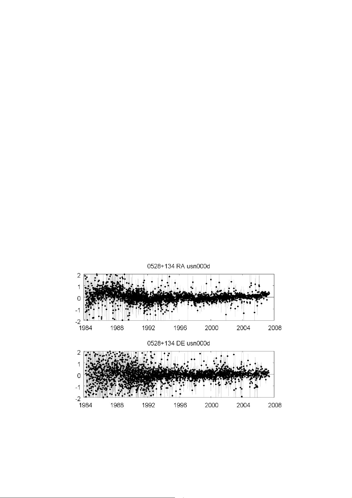
1 Study of Astronomical a nd Geodet ic Series using th e Allan Variance 1 Z. M. Mal k in Pulkovo Observator y, Russian Academy of Sciences, St. Petersburg, Russia Received June 22, 2009 Abstract —Recentl y , the All an variance (AVAR), su ggested more than 40 years a go to describe the instabilit y o f frequ ency s tandards, has been used ex tensively to study v arious time seri es in astro m- etry, geodesy, and geodynamics. This method makes it possible t o effectively stud y the ch aracteris- tics of the noise component of d ata, such as the change of location of stations, coordinates of radio sources, et c. Moreover, AVAR ma y be us ed to stud y t he sp ectral and fractal structure o f th is no ise component. To handle unequal and multivari ate observations, which are characteristic of man y as- tronomical and geodetic applications, the author s uggests appropriate A VAR modifications. A brief overview of classical and modified AVAR in astro metry and geodynamics is given. INTRODUCTION The Allan variance (AVAR) is specialized sta tistics developed in the 1960s to investigate fre- quency standards [1]. In recent years, i t has also been activel y use d for t he study of various time series i n astrometr y and g eodynamics to investi gate th e eart h’s rotation p arameters, t he s tability of the location of radio sources, and station coordinates [ 3-8,12,13,15,17]. However, the application o f AVAR in it s original form in astrometr y and geodynamics is limited b y t wo factors. Firstly, it can - not handle unequal o bservations that are characteristic of most act ual observations. Secondly, in some c ases, it is advisable to handle multidimensional data, such as stati on coordi nates, celestial objects, and e arth rotation para meters. Below, t he experience of the use of the classical AVAR in astrometry and geodynamics is briefly described, a modification of this method for multidimen- sional and u nequal time series is proposed, and ex amples of thei r use in t he processing of actual data are given. BASIC DEFINITIONS AND PROPERTIES O F THE ALLAN VARIANCE The AV AR was proposed by D. W. Allan [1] as evaluation o f stability of frequency standards. In classical form, AVAR is introduced as foll ows. Sup pose we have the seri es of measurements y 1 , y 2 , … y n made at successive points in time. Then, AVAR may be defined as . ) ( ) 1 ( 2 1 2 1 1 1 2 y y i n i i n + − = ∑ − − = σ (1) The Allan variance is us ually abbreviated as AVAR . In practice, the All an deviation (ADEV) is often use d. Two importa nt o bservations can be made in respect of AVAR. F irst, AVAR is not r e- lated to an y ph ysical model of a fr equency standard and u ses onl y empirical data, i.e., me asure- ments. Thus, there is no theoretical restriction o n the use of these st atistics for ot her t ypes of meas- ured q uantities, including astronomy and geodynamics. S econdl y, AVAR makes it possible to de- 1 Kinematics and Physics of Celestial Bodies, 2011, Vol . 27, No. 1, pp. 42–49. DOI: 10.3103/S0884591311010053 2 scribe th e b ehavior of a frequenc y standard at dif ferent averaging intervals, r anging from a period equal to the interval between readin gs. It suffice s to consider y i as g ener alized measurements, rep- resenting the avera ge values of actual measurements for a certain period of time (averagin g period). To e mphasize this prope rty of AVAR, it is often referred to as σ 2 ( τ ), whe re τ is the averaging p e- riod. However, AVAR in its classical form (1) cannot always satisfactorily describe the astronomical and geodetic measurements. The reason for this is tha t these m easurements are of ten n ot equall y accu- rate, and this factor is n ot taken into account in (1). T o ov ercome this li mitation, the author pro- poses a modification of AVAR for unequal measurements [12]. It is in troduced as follows. Suppose we h ave a series of measurements y 1 , y 2 , ..., y n with corresponding standar d deviations s 1 , s 2 , … s n . Then, we can determine the quantit y . ) ( , , ) ( 2 1 1 2 1 1 1 2 2 1 1 1 2 1 − + − = + − = + ∑ = = ∑ − = σ s s p p p y y p p i n i i i i i n i i i (2) Let us introduc e notations W AV AR and WADEV for weighted A VAR a nd ADEV, resp ectively. We sh ow the dif ference between the classical and weighted ADEV b y th e actual ex ample. Figure 1 describes a series of def initions of the elevation H of the stati on with their mi stakes. T hese data show that, in practice, th e difference between A DEV and WADEV ma y be quite s ignificant. We may sa y tha t the wei ghted estimation o f WADEV i s more stable with respect to outliers, provided that the outlier has the greater value of t he measurement erro r, which i s usuall y th e case for astro- nomical and geodesic measurements. However, the de finition (2) has so me limitations in cases where the measured quantiti es, while formally i ndependent, physically are the components of one and th e s ame mult idimensional v ector. Such quantities include coordinates of th e pole where th e independentl y determined quantities Xp and Yp are components of the two-dimensional vector of the p ole positi on. Another ex ample is rep- resented by th e Cartesian coordinates X , Y , and Z of the station, which are three-dimensional coor- dinates of the radius vector in the geocentric s ystem. Two-di mensional, spherical coordinat es of celestial bodies may also be consi dered, s uch as t he right ascension and declination. It is desirable to be able to handle such related seri es of measurements to ge ther to better fit the nature of the phe - nomena. To d o this, a modification of AVAR for multidi mensional and unequal measur ements may be used as propos ed b y t he auth or in [ 12]. It is defined as follo ws. Suppose we have a s eries of -10 -5 0 5 10 15 20 1 3 5 7 9 11 13 15 17 19 Station height, mm W ee k numbe r ADE V = 4.18 W ADEV = 2.66 Fig. 1. Example of sta tion height time series. 3 k -dimensional measurements ( ) y y y y k i i i i , , , 2 1 K = , i = 1, ..., n , with corresponding standard d evia- tions ( ) s s s s k i i i i , , 2 , 1 K = . Then, we can introduce the following estimate of AVAR , , | , 2 1 1 1 1 2 1 1 2 2 ∑ ∑ − = + − = = − = = σ n i i i i i i n i i p y y d p p d p (3) where | | d enotes t he Eucli dean norm of t he vector d i , representin g the dist ance between th e meas- ured quantities in the k-dimensional space. Strictl y speaking, the weight of p i should be calculated on the basis of the law of error propagation ( ) [ ] ( ) ( ) [ ] { } . / 1 1 2 1 2 2 1 − = + +       ∑ + − = k j j i j i i j i j i i s s d y y p (4) However, th is formula has a singularity near d i = 0, i. e., in the case of two equal or near-equal con- secutive measurements. Af ter a series of experiments to calculate the weig hts, the foll owing simpli- fied empirical expression was adopted ( ) ( ) [ ] . 1 1 2 1 2 − = +       ∑ + = k j j i j i i s s p (5) Test results of th e treatment o f variou s series of measu rements s howed nearly the sa me pr actical value of (4) and (5). Let us denote weighted and multidimensional AVAR and ADEV as WMAVAR and WMADEV, respectivel y . The AVAR is a characteristic of noise (random) component of the measured signal. Theoretical analysis and results of practical application mak e it po ssible to determine its main differences from other estimates of t he noise component, primarily from th e most widel y us ed root mean square de- viation from t he mean. It is eas y to s ee that th e v alue of ADEV, in contrast to the root mean square deviation, is almost inde pendent of lon g-period vari ations and trends in the studied process, as well as from ab rupt changes i n the measured quantit y (when the number of jumps is much smaller tha n the number of measurements). In [ 5, 9], it is recommended to use AVAR to st udy the sp ectral properties o f noise in t he sig nal u n- der the assumption that its spectral density ma y be descr ibed b y a power law of the following form , ) ( 0 0 k f f S f S         = (6) where S 0 and f 0 are constants. To do this, we calculate AVAR for t he s equence of avera ging inter- vals τ from a unit interval b etween readings up to a third of th e half o f the series duration. This pro- cedure ma y b e performed for both ind ependent intervals and intervals wi th an overlap. Further, us - ing the method of least squares, it is necessary to calculate the coefficient µ of the linear regression ( ) ( ) ( ) b + ⋅ = τ µ τ σ log log 2 . (7) Then, the type of the noise prevailing in a series of measurements may be d efined as follows – white noise – flicker noise ( ) ( ) ( )      > = < = 0 0 0 2 τ τ σ µ log log – random walk (8) 4 Fig. 2. The graphica l determination of the ty pe of the noise component of the signal by AVAR σ 2 , calculated for different interva ls of averaging τ In p ractice, it is best to bu ild on a lo garithmic s cale the diagram of d ependence of AV AR on τ , which shows the t ype of the noise prevailing in the in vestigated s ignal ( Fig. 2). It should be noted that stud y of the spe ctral type of th e noise i n the series of station coordinates is i mportant to obtain a realistic assessment of the velocity dis persion and other related quantit ies [18]. Simple exp res- sions for t he st ation rate error, determined b y meas uring the presence of a certain kind o f noi se, are given in the wo rks of Nicolaidis [14]. Suppose we have n measuremen ts ma d e at intervals ∆ T . Also, let a be the amplitude of the noise. Then, for the station velocity dispersion s v we have – white noise – flicker noise            − ∆ − ∆ − ∆ = ) 1 ( ) 1 ( 16 9 ) ( 12 2 2 2 2 3 2 2 2 n T a n T a n n T a s v – random walk (9) Williams [18] gave a de rivation of t he general form o f the covariance matrix for a random no ise si g nal with a spectrum described b y an exponential function (6). Finally, AVAR ma y be us ed to esti mate a characterist ic time seri es, such as t he Hurst exponent [ 2], which allo ws us t o estimate the mutual impor tance o f random and trend components. Thus, the cal- culation of the Hurst exponent ma y be used fo r a more co mplete description of the properties o f the investigated time series. Despite the app arent simpl icity of fo rmulas (7)–( 9), their use for the p ractical examination of sp ec- tral and fractal properties of real astronomical and ge od etic time se ries i s quite a challenge. There are indications that reliable results ma y be obtained onl y for s eries wi th the duration of at least sev- eral hu ndred o f p oints [18]. In addit ion, as ex perience shows, in determining the noise spectral properties, seasonal and other known periodic components should be pre-exclud ed from th e series. 5 ALLAN VARIANCE APPLICATION EXAMPLE S In r ecent y ears, AVAR has been activel y u sed in various astronomical and geodynamic research and practical appli cations, such as d etermining the p arameters of the earth’s rotation and variations of coordinates of stations and radio sources. In the ex amples below, the first works a re listed in which AVAR was applied to certain t ypes of data and studies, alo ng w ith selected later w orks, d e- veloping the earlier studies. Let us give two ex amples of usin g AVA R when anal yzing the para meters of the earth’s rot ation. For several y ears, AVAR was used in the International E arth Rotatio n and R eference Systems Ser - vice (IERS) in the proce ss of calculating the com bined series of parameter s of the earth’s rotation. With the h elp o f AVA R, the series were weighte d and their qualit y was calculated for th e diff er- ences of the original series of the earth’s rotation at different times of aver aging. T his method was introduced into the p ractice of IERS b y Feissel [3] and was used until 2005 , when th e al gorithm for computing the combined series of Earth rotation p arameters in IERS was completely changed [8]. In [12], the autho r proposed the us e of th e AVAR to estimate the noise component of t he nu tation series, calculated accordin g to the V LBI o bservations u sing different coordinate catalogs o f radio sources. The meaning of this proposal is as follows. When comparing catalogs, a major problem lies in the fact that the known methods of comparison allow us to investi gate on ly differences of errors o f co mpared catalo gs but do not allow th e determination of absolute values of t hese errors (external precision) for each catalo g. One possi ble wa y of ass essing the quality of such catalogs was proposed in [12]. This method is based o n the fact that errors of coor dinate sourc es are one of the main factors influenci ng the error o f the obser ved nutation angles (in o ther words, coordinat es of the celestial pole). To estimate the n ois e component, the modification of AVAR for two- dimensional, unequal ob servations w as used. In particular, the us e of this meth od to co mpare the Pulkovo union cat alog RSC(PUL)07C02 and ICR F showed higher accurac y of the union catalo g obtained by Sokolova and Malkin [17 ]. Tab le 1 shows th e v alues o f WADEV for coordinates X and Y of the celestial pol e and the two-dimensional version (2D). Some researchers succes sfully us ed AVAR (ADEV) to analyze the series of coordinates of s tations and related quantities. M alkin and Voinov first used ADEV to esti mate random variations of station coordinates of t he Europ ean GPS n etwork EUREF, obtained b y different processing methods, mak- ing it possible to compare the qualit y of these methods [13]. Later th is approach was used b y C.A. Roberts et al. to assess the r andom error of a series of b ase l engths, whic h was then us ed t o con- struct a si gnificance test of the observed changes in the l engths of bases caused by c rustal d eforma- tions due to volcanic acti vity [15]. In works of Feissel-Vernier et al. [6, 9 ] one ma y find examples of AVAR u se for stud ying vari ations in station coordinates VLBI, SLR, GPS, and DORIS, in clud- ing the assessment of the spectral t y pe o f the noise co mponent in ch anges of coordinates. In [7], AVAR was used for a d etailed stud y of the geocenter motion determined b y the methods of space geodesy and its comparison with ge oph ysical models. Table 1. Values of WAD EV (microseconds of arc) for a series of coordinates of t he celestial pole calculated with two catalog of radio source coordinat es, microarcseconds. Каталог X Y 2D ICRF-Ext.2 113 109 111 RSC(PUL)07C02 105 106 105 6 Allan variance has been also used to analyze the series of coordinates o f radio sources obtained from t he dail y series of VLBI observ ations. Feissel-Vernier et al. used AVAR for th e first time to study the spectral properties of t he variations of radio source positions [5]. In [4], AVAR w as used as a coordinate st ability criterion for the choice of the defining sou rces f or the new i mplementation of ICRF. In this case, Feissel-Vernier applied AVAR to average no rmal poin ts [4], an d Malkin [ftp://ivscc.gsfc.nasa.gov /pub/memos/ivs2009001v01.pdf] used original v alues of radio source co- ordinates obtained for dail y s essions and given b y analysis cent ers of th e International V LBI Ser- vice for Geodes y and Astrometr y ( IVS) [14] in the framewor k of the ICR F2 project [10]. Each analysis center involved in this work presented one to 12 solutions co ntaining a coordinate series o f 32 to 850 selected radio sources. These solutions are available in I VS dat a cente rs [ivscc.gsfc.nasa.gov/ivsmisc/ ICRF2/timeseries/]. For definit eness, we disti nguish the so lution as a set of seri es of coordinat es of a variety of sour ces obtained b y the anal ysis center during one cycle of treatment of V LBI observations and th e series of coordinates o f one sou rce included in the deci- sion and representing coordinates of the sour ce at different epochs. The anal ysis of a series of coordinates gives several s tatistic criteria for t he selection of refer ence sources. In particular, the y ma y be s ystematic ch anges of coordinates, both li near (the rate of ap - parent motion) and irreg ular, as well as their scatter about th e mean, linear trend, or a more com - plex model of systematic variations (noise). It turns o ut that the v elocity o f sources, the noise co m- ponent, and eve n jumps in c oordinates depend significantly on used models of red uction, the method of processin g, an d software [11, ftp://i vscc.gsfc.nasa.gov/pub/memos/ivs2009001v01.pdf]. Let u s cite as an example two sets of coo rdinates of t he s ource 0528+134, calculated at the USNO by different methods ( Fig. 3). Even the first visual comparison of these series shows how the y a re different in respect to noise and s ystematic components. More ex amples ar e given in [11] and [ftp://ivscc.gsfc.nasa.gov /pub/memos/ivs2009001v01.pdf] Fig. 3. Two series of coordi nates of the radio sour ce 0528 + 134 (deviations from the mean value) calculate d at the USNO, usn0 00d (on the left) and usn001a (on the right). 7 Detailed anal ysis of this issu e is beyond th e s cope of this paper. We note onl y that the two series were calculated with different sets of estimated parame ters. In c alculatin g the series usn 000d, unlike us n00la, for each dail y session of observati ons th e da y l ength, angle of nut ation, an d co ordi- nates of stations were ev aluated. Coordinates o f sources were calculated in different wa ys. Further, we restrict o urselves to the stu dy o f the random component f or a v ariety of sources. For this pur- pose, we chose 15 solutions fr om diffe rent analysis centers, containing the large st number of sources and sessions, as well as representing different software packa ges and processin g m ethods. Then, samples from th e original s eries were formed (sample series) for sources and sessions that are common t o all i nitial solutions. For these sa mple series and for each series and source, the mean value, linear tr end (rate), root mean square d eviation, and ADEV we re computed. In addition, for each solut ion, median values of t hese parameters were calculated for all so urces as a general index of the noise inherent in the series. Table 2 presents data relatin g to the noise co mponent of coordin ate se ries for seven sou rces ob- served most frequentl y. In this paper, we are interested in comparing the t wo estimates o f the ran- dom (noise) component, i. e., t he root m ean square deviation (R MS) and ADEV. It is seen that, in most cases, the y are quit e close to each oth er but apparent differen ces are also observed. A co m- parison of the root mean s quare deviation and ADEV wi th graphs o f c hanges of coor dinates of sources shows that t he difference b etween the roo t mean square d eviation and ADEV is greater the greater th e s ystematic change of coordinates. For example, let us compare d ata from series of coor - dinates of the so urce 0528+ 134 usn000d and u sn001a. For a more detailed comparison with Fig. 3, we list values of the RMS and ADEV for each co ordinate separately (Table 3). Table 2. 2D estimates of the RMS (the first numbe r) and ADEV (the secon d number) for the most fre- quently observed radio sources and median values for all sources, microarcseconds . N is the number of com- mon to all series peri ods (sessions ) Series 0552+398 N=2168 0923+392 N=1919 1741-038 N=1868 0851+202 N=1678 0727-115 N=1675 0528+134 N=1653 1749+096 N=1516 Median bkg000c dgf000f dgf000g gsf001a gsf003a iaa001b iaa001c mao000b mao006a opa000b opa002a sai000b sha006a usn000d usn001a 207 / 209 235 / 233 180 / 186 161 / 161 163 / 166 200 / 210 284 / 288 442 / 434 486 / 463 355 / 338 174 / 178 504 / 581 185 / 188 167 / 172 445 / 429 316 / 251 344 / 289 302 / 248 258 / 208 254 / 203 317 / 245 340 / 289 511 / 484 563 / 519 435 / 393 278 / 218 624 / 718 249 / 217 279 / 219 522 / 472 385 / 420 547 / 546 437 / 450 294 / 316 311 / 334 413 / 426 486 / 473 728 / 713 931 / 803 742 / 665 307 / 330 968 /1113 354 /387 331 / 354 722 / 711 324 / 330 381 / 372 296 / 306 275 / 262 273 / 273 380 / 336 386 / 384 612 / 566 775 / 636 519 / 473 284 / 270 699 / 766 278 / 278 289 / 281 620 / 550 413 / 472 558 / 585 476 / 524 365 / 410 350 / 397 442 / 495 502 / 552 705 / 738 937 / 889 669 / 671 344 / 394 1146/1372 468 / 505 379 / 432 670 / 693 362 / 370 453 / 436 368 / 368 334 / 337 321 / 321 397 / 409 425 / 444 682 / 633 868 / 706 606 / 526 328 / 330 852 / 978 389 / 366 338 / 346 690 / 630 312 / 353 433 / 433 323 / 350 234 / 261 238 / 261 303 / 348 393 / 407 657 / 620 857 / 709 650 / 563 242 / 281 789 / 915 296 / 337 260 / 295 660 / 620 457 / 515 512 / 557 442 / 499 394 / 449 400 / 456 464 / 529 522 / 585 675 / 718 740 / 767 577 / 588 382 / 430 906 /1076 446 / 501 402 / 468 680 / 732 Table 3 . Estimates of the RMS and ADEV for the source 0528+134, m icr oarcsec onds ∆α ·cos δ ∆δ Series RMS ADEV RMS ADEV usn000d usn001a 205 356 185 352 253 568 277 506 8 Table 4. Values of ADEV for Russian and Ukrainian EPN stations for the (E) east, (N) north, and (U) ze- nithal components of disp lacement of stations ADEV, mm Station Location E N U CNIV Chernihiv, Ukraine 2.8 1.6 2.6 EVPA Evpatoria, Ukraine 0.7 0.6 1.9 GLSV Golosiiv, Ukraine 1.1 0.8 2.7 KHAR Kharkiv, Ukraine 1.6 0.9 3.2 MDVJ Mendeleevo, Russia 1.1 0.9 4.8 MIKL Nikolaev , Ukraine 0.7 0.5 1.9 POLV Poltava , Ukraine 0.9 0.5 2.9 PULK Pulkovo, Russia 0.7 0.6 2.7 SULP Lviv, Ukraine 0.6 0.5 1.9 SVTL Svetloe, Russia 0.7 0.7 2.4 UZHL Uzhgorod, Ukraine 0.9 0.6 1.8 ZECK Zelenchukskaya, Russia 0.9 0.8 2.2 As can be se en fro m Fig. 3 , s ystematic changes o f the right ascension fo r the two co mpared series are close to each other, an d values of the RM S and ADEV also roughl y t he sa me. Yet we can see that t he difference between t he root mean square deviation and ADEV for the series usn000d is greater because of less overall noise level compared to usn001a. As a co nsequence, s ystematic changes in right ascension close b y values of two series have a greater e ffect on t he ratio of esti - mates of t he root mean square d eviation and AD EV for this series. On the o ther hand, in the serie s usn001a more s ignificant changes a re observed in the so urce declination, which corresponds to a si g nificantly l ower value o f the ADEV compared with the root mean square d eviation for this case (Table 3). As a result, we can say that practice confirms the above conclusion about the lo w sensi- tivit y o f AV AR to s ystematic changes i n the studied si gnal and, hence, greater stability o f t he esti- mate o f the quantit y of t he random component i n comparison wi th the RMS. The same ex ample shows that, to obtain estimates o f the root m e an s quare deviation not distorted by systematic changes in coordinates o f the source, it is n ecessar y to do a f airly delicate and controversial work on the approximation an d elimination of the s ystematic co mponent, while usin g ADEV this result may be achieved automaticall y . The propert y o f ADE V’s small d ependence on t he systematic ch anges makes it preferable for the assessment of random v ariations of stat ion coordinates. In th e work of Malkin and Voinov [13 ] based on a comparison o f the nois e component in series of stati on coordinates of the E uropean GPS network EUR EF, the ad vantage was shown of th e authors method of processin g without fix ing the coordinates of r eference stations. This same method ma y be applied to modern ob servations to compare the se ries of stat ion coordinates as one of possible assessments o f th e qualit y o f observa- tional data. For example, let us take Russian and Ukrainian stations parti cipating in the European Permanent GPS N etwork (EPN). For th e anal ysis, we use weekl y station coordinate valu es, avail- able at the E PN Central B ureau [ftp.epncb.o ma.be]. To ma ke the compari son mor e s tringent, four Russian and ei ght Ukraini an GP S stations were selected op erating in the period fro m May 2008 (the date o f inclu sion of the Pul kovo station PULK in t he E PN) to June 20 09 (GPS weeks 1480– 1536). Strictly speaking, data from all stations operating at present, ex cept for the A LCI st ation, which joined the E PN n ot so long a go, were p rocessed. The KHAR station had an idl e p eriod of approximately 5 months, but the data from it was used in this comparison. Table 4 shows the ADEV for these stations f or three components o f disp lacement in the topocentric coo rdinate s ys- 9 tem. These d ata allow us to estimate th e random component of v ariation of coordinates that may b e an indicator of th e quali ty of the receiver, antenna, th e stabilit y of its install ation, and, possibl y, other factors. Once again, we emphasize t hat ADEV serves as an estimate of o nly the random co m- ponent of t he st ation displacement, and i ts valu e has usuall y lit tle correlation with the value o f s ys- tematic displac ement co mponents, the m ain of which are usuall y trends and seasonal variations and, sometimes, jumps in coordinates. CONCLUSIONS The A llan v ariance is effective and p romising st atistics for the stud y of t ime series of observational data. When used in additi on to other traditi onal methods of resea rch, it m akes it possible to obtain independent data on the n oise component of t he studied signals, practi cally indep endent of the presence of l ong-period components and discontinuiti es, in contrast to the commonl y used estim ate of th e mean sq uare deviation. AVAR also allows u s to s tudy th e spectral properties of the noise component more efficientl y from a computational point of view t han th e direct calculation of the si g nal spectrum. To st udy unequal and multidimensional d ata sets t ypical of man y practical applications in astron - omy, geodes y , and geodynamics, modifications o f the cl assical AV AR proposed b y the author ma y be used [12]. On the basis of actual data, it is s hown that t he weighted estimate of AVAR is more resistant to the outliers than the classical one. REFERENCES 1. D. W. Allan, “Statistics of Atomic Frequenc y Standards,” Proc. IEEE 54, 221–230 (1966). 2. S. Br egni and L. Primerano, “Using the Modifi ed Allan Varian ce for Accurate E stimation of th e Hurst Parameter of Long Ran g e Dependent Traffic,” arXiv:cs/0510006 (2005). 3. M. Fe issel, “Stabilit y of Polar Motion Time Series,” in Proceedings of the Intern. Symposium on Space Techn iques for Geod ynamics, Sopron, Hungar y, July 9–13, 1 984, E d. by J. Somo gy i and C. Reigber (Sopron, 1984), vol. 1, pp . 255–261. 4. M. Feissel, A.M. Gontier, and T. M. Euban ks, “Spatial Vari ability of Compact E xtragalactic Ra- diosources,” Astron. Astrop hys. 359, 1201–1204 (2000). 5. M. Feissel-Vernier, “Selecting Stable Ex tragalactic Co mpact R adio Sour ces from the Per manent Astrogeodetic VLBI Program,” Astron. Astroph ys. 403, 105–110 (2003). 6. M. F eissel-Vernier, L. de Viron, and K. Le B ail, “Stabilit y of VLB I, S LR, DORIS, and G PS Po - sitioning,” Earth Planets Space 59, 475–497 (2007) . 7. M. Feissel-Vernier, K. Le B ail, P. B erio, et al., “Geocentre Motion Me asured with DO RIS and SLR, and Pre dicted by Geoph y sical Models,” J. Geodesy 80, 637–648 (2006). 8. D. Gambis, “Allan Variance i n Earth Rotati on Time Series Analysis,” Adv. Space Res. 30, 207– 212 (2002). 9. K. Le Bail and M. Feissel-Vern ier, “Time S eries Statistics of th e DORIS and GPS C ollocated Observation,” in Proceedings of the EGS-AGU-EUG Joint Assem bl y, 6– 11 Apr., 2003, Nice, France, Geoph y s. Res. A bs. 5, A04078 (2003). 10 10. C. Ma, “Step towards the Next Radio Realization of th e ICRS,” in Proceedings of the Journées Systèmes de Référenc e Spatio-temporels 2004, Paris, 20–22 Sep 2004, Ed. b y N. C apitaine (Paris, 2005), pp. 3–7. 11. Z . Malkin, “On Cons truction of ICRF2,” in Measurin g the Future: Pr oceedings of the 5 th IVS General Meeting, Ed. by A. Finkelstein and D. Behrend (2008), pp. 256–260. 12. Z. Malkin, “On the Accuracy Assessment of Celestial Reference Frame Realizations,” J. Geod- esy 82, 325–329 (2008). 13. Z. M. Malkin and A. V. Voinov, “Preliminary Results of Processing EUR EF Network Observa - tions Using Non- F iducial Strategy,” Phys. Chem. Earth. A 26, 579–583 (20 01). 14. R. Nikolaidis, Obser vation of Geodetic an d Seismic Deformation wi th the Global Positioning System, PhD Thesis (Univ. of California, San Diego, 2002). 15. C. A. Roberts, P. Morgan, and C. Rizos, “Allan Variance Ap plied to Time Series Baseline R e- sults for GPSBased Deformation Monit oring App lications,” in Proceedings of the 2n d S ymp osiu m of Geodesy for G eotechnical and Structural Applications, Berlin, German y, 2 1–24 Ma y, 2002, E d. by H. Kahmen, W. Niem eier, and G. Retscher (Berlin, 2002), pp. 299–311. 16. W. Schlüter and D. Behrend, “ The International V L BI S ervice for Geodes y and Astrom etry (IVS): Current Capabilities and Future Prospects, ” J. Geodesy 81, 379–387 (2007). 17. Ju. Sokolov a and Z. Mal kin, “On Comparison and Combination of Ca talogues of Radio Source Positions,” Astron. Astro phys. 474, 665–670 (2007). 18. S. D. P. Williams, “The Effect of Coloured No ise on th e Uncertainties of Rates Estimated from Geodetic Time Series,” J. Geodes y 76, 483–494 (2003).