Implementation of an Optimal First-Order Method for Strongly Convex Total Variation Regularization

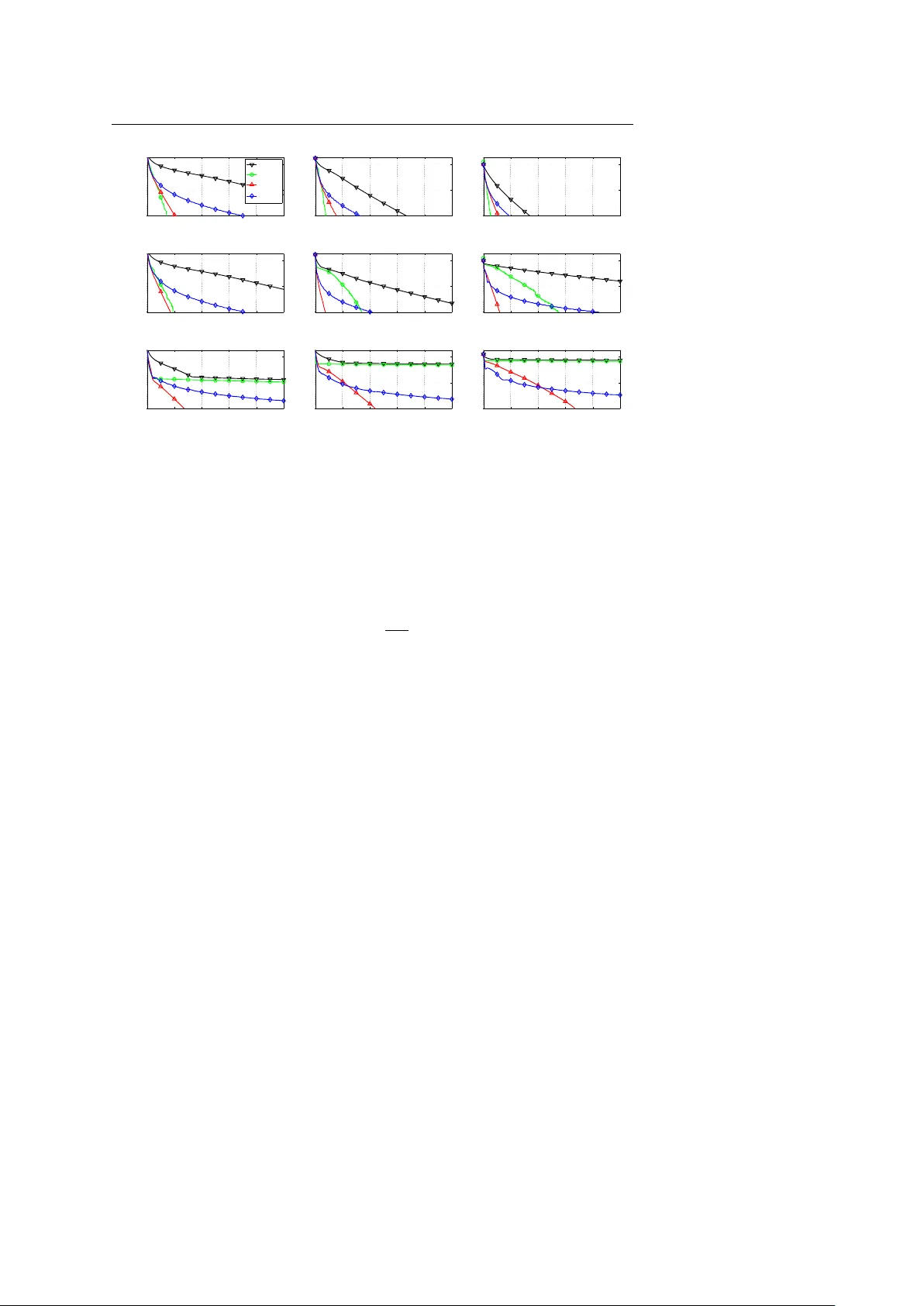
Noname manuscript No. (will be inserted by the editor) Implementation of an Optimal First-Order Method f or Strongly Con vex T otal V ariation Regularization T . L. Jensen · J. H. Jørgensen · P . C. Hansen · S. H. Jensen Receiv ed: date / Accepted: date Abstract W e present a practical implementation of an optimal first-order method, due to Nesterov , for large-scale total variation regularization in tomographic recon- struction, image deblurring, etc. The algorithm applies to µ -strongly con ve x objecti ve functions with L -Lipschitz continuous gradient. In the framework of Nesterov both µ and L are assumed known – an assumption that is seldom satisfied in practice. W e propose to incorporate mechanisms to estimate locally sufficient µ and L during the iterations. The mechanisms also allow for the application to non-strongly con vex functions. W e discuss the iteration complexity of sev eral first-order methods, inclu- ding the proposed algorithm, and we use a 3D tomography problem to compare the performance of these methods. The results sho w that for ill-conditioned problems solved to high accuracy , the proposed method significantly outperforms state-of-the- art first-order methods, as also suggested by theoretical results. Keyw ords Optimal first-order optimization methods · strong conv exity · total variation re gularization · tomography Mathematics Subject Classification (2000) 65K10 · 65R32 1 Introduction Large-scale discretizations of in v erse problems [20] arise in a v ariety of applications such as medical imaging, non-destructi ve testing, and geoscience. Due to the inher- This work is part of the project CSI: Computational Science in Imaging, supported by grant no. 274-07- 0065 from the Danish Research Council for T echnology and Production Sciences. T obias Lindstrøm Jensen, Søren Holdt Jensen Department of Electronic Systems, Aalborg Uni versity , Niels Jernesvej 12, 9220 Aalborg Ø, Denmark. E-mail: { tlj,shj } @es.aau.dk Jakob Heide Jørgensen, Per Christian Hansen Department of Informatics and Mathematical Modelling, T echnical University of Denmark, Building 321, 2800 L yngby , Denmark. E-mail: { jakj,pch } @imm.dtu.dk 2 T . L. Jensen, J. H. Jørgensen, P . C. Hansen, and S. H. Jensen ent instability of these problems, it is necessary to apply regularization in order to compute meaningful reconstructions, and this work focuses on the use of total varia- tion which is a powerful technique when the sought solution is required to have sharp edges (see, e.g., [12, 33] for applications in image reconstruction). Many total variation algorithms have already been developed, such as time march- ing [33], fixed-point iteration [37], and various minimization-based methods such as sub-gradient methods [1, 13], second-order cone programming (SOCP) [18], duality- based methods [8, 11, 22], and graph-cut methods [9, 16]. The difficulty of a problem depends on the linear operator to be in verted. Most methods are dedicated to denoising, where the operator is simply the identity , or possibly deblurring of a simple blur, where the operator is in v ertible and represented by a fast transform. For general linear operators with no exploitable structure, such as in tomographic reconstruction, the selection of algorithms is limited. Furthermore, the systems that arise in real-world tomography applications, especially in 3D, are so large that memory-requirements preclude the use of second-order methods with quadratic con ver gence. Recently , Nesterov’ s optimal first-order method [27, 28] has been adapted to, and analyzed for, a number of imaging problems [14, 38]. In [38] it is shown that Nes- terov’ s method outperforms standard first-order methods by an order of magnitude, but this analysis does not cov er tomography problems. A drawback of Nestero v’ s al- gorithm (see, e.g., [10]) is the explicit need for the strong conv exity parameter and the Lipschitz constant of the objectiv e function, both of which are not a v ailable in practice. This paper describes a practical implementation of Nesterov’ s algorithm, aug- mented with ef ficient heuristic methods to estimate the unknown Lipschitz constant and strong con ve xity parameter . The Lipschitz constant is handled using backtrack- ing, similar to the technique used in [4]. T o estimate the unknown strong con ve xity parameter – which is more difficult – we propose a heuristic based on adjusting an estimate of the strong con ve xity parameter using a local strong con vexity inequality . Furthermore, we equip the heuristic with a restart procedure to ensure con ver gence in case of an inadequate estimate. W e call the algorithm UPN (Unkno wn Parameter Nesterov) and compare it with two versions of the well-known gradient projection algorithm; GP : a simple version using a backtracking line search for the stepsize and GPBB : a more advanced version using Barzilai-Borwein acceleration [2] and with the backtracking procedure from [19]. W e also compare with a variant of the proposed algorithm, UPN 0 , where the strong con vexity information is not enforced. This v ariant is similar to the FIST A algorithm [4]. W e have implemented the four algorithms in C with a MEX interface to MA TLAB, and the software is a v ailable from www2.imm.dtu.dk/ ~ pch/TVReg/ . Our numerical tests demonstrate that the proposed method UPN is significantly faster than GP , and as fast as GPBB for moderately ill-conditioned problems, and significantly faster for ill-conditioned problems. Compared to UPN 0 , UPN is con- sistently faster , when solving to high accurac y . W e start with introductions to the discrete total v ariation problem, to smooth and strongly conv ex functions, and to some basic first-order methods in Sections 2, 3, and 4, respectively . Section 5 introduces important inequalities while the new algorithm A First-Order Method for Strongly Con vex TV Re gularization 3 is described in Section 6. The 3D tomography test problem is introduced in Section 7. Finally , in Section 8 we report our numerical tests and comparisons. Throughout the paper we use the following notation. The smallest singular value of a matrix A is denoted σ min ( A ) . The smallest and largest eigenv alues of a symmetric semi-definite matrix M are denoted by λ min ( M ) and λ max ( M ) . For an optimization problem, f is the objective function, x ? denotes a minimizer , f ? = f ( x ? ) is the opti- mum objectiv e, and x is called an ε -suboptimal solution if f ( x ) − f ? ≤ ε . 2 The Discrete T otal V ariation Reconstruction Problem The T otal V ariation (TV) of a real function X ( t ) with t ∈ Ω ⊂ R p is defined as T ( X ) = Z Ω k ∇ X ( t ) k 2 d t . (2.1) Note that the Euclidean norm is not squared, which means that T ( X ) is non-dif feren- tiable. In order to handle this we consider a smoothed version of the TV functional. T wo common choices are to replace the Euclidean norm of the v ector z by either ( k z k 2 2 + β 2 ) 1 / 2 or the Huber function Φ τ ( z ) = ( k z k 2 − 1 2 τ if k z k 2 ≥ τ , 1 2 τ k z k 2 2 else . (2.2) In this work we use the latter , which can be considered a prox-function smoothing [28] of the TV functional [5]; thus, the approximated TV functional is giv en by T τ ( X ) = Z Ω Φ τ ( ∇ X ) dt . (2.3) In this work we consider the case t ∈ R 3 . T o obtain a discrete version of the TV reconstruction problem, we represent X ( t ) by an N = m × n × l array X , and we let x = vec ( X ) . Each element or voxel of the array X , with index j , has an associated matrix (a discrete differential operator) D j ∈ R 3 × N such that the vector D j x ∈ R 3 is the forward difference approximation to the gradient at x j . By stacking all D j we obtain the matrix D of dimensions 3 N × N : D =    D 1 . . . D N    . (2.4) W e use periodic boundary conditions in D , which ensures that only a constant x has a TV of 0. Other choices of boundary conditions could easily be implemented. When the discrete approximation to the gradient is used and the integration in (2.3) is replaced by summations, the discrete and smoothed TV function is giv en by T τ ( x ) = N ∑ j = 1 Φ τ ( D j x ) . (2.5) 4 T . L. Jensen, J. H. Jørgensen, P . C. Hansen, and S. H. Jensen The gradient ∇ T τ ( x ) ∈ R N of this function is giv en by ∇ T τ ( x ) = N ∑ j = 1 D T j D j x / max { τ , k D j x k 2 } . (2.6) W e assume that the sought reconstruction has v oxel v alues in the range [ 0 , 1 ] , so we wish to solve a bound-constrained problem, i.e., ha ving the feasible region Q = { x ∈ R N | 0 ≤ x j ≤ 1 } . Given a linear system A x ≈ b where A ∈ R M × N and N = mnl , we define the associated discr ete TV r e gularization problem as x ? = argmin x ∈ Q φ ( x ) , φ ( x ) = 1 2 k A x − b k 2 2 + α T τ ( x ) , (2.7) where α > 0 is the TV regularization parameter . This is the problem we want to solve, for the case where the linear system of equations arises from discretization of an in verse problem. 3 Smooth and Strongly Con vex Functions T o set the stage for the algorithm de velopment in this paper , we consider the con vex optimization problem min x ∈ Q f ( x ) where f is a conv ex function and Q is a con ve x set. W e recall that a continuously differentiable function f is con ve x if f ( x ) ≥ f ( y ) + ∇ f ( y ) T ( x − y ) , ∀ x , y ∈ R N . (3.1) Definition 3.1 A continuously dif ferentiable con vex function f is said to be str ongly con ve x with str ong con ve xity parameter µ if there exists a µ ≥ 0 such that f ( x ) ≥ f ( y ) + ∇ f ( y ) T ( x − y ) + 1 2 µ k x − y k 2 2 , ∀ x , y ∈ R N . (3.2) Definition 3.2 A continuously dif ferentiable conv ex function f has Lipschitz contin- uous gradient with Lipschitz constant L , if f ( x ) ≤ f ( y ) + ∇ f ( y ) T ( x − y ) + 1 2 L k x − y k 2 2 , ∀ x , y ∈ R N . (3.3) Remark 3.1 The condition (3.3) is equiv alent [27, Theorem 2.1.5] to the more stan- dard way of defining Lipschitz continuity of the gradient, namely , through con vexity and the condition k ∇ f ( x ) − ∇ f ( y ) k 2 ≤ L k x − y k 2 , ∀ x , y ∈ R N . Remark 3.2 Lipschitz continuity of the gradient is a smoothness requirement on f . A function f that satisfies (3.3) is said to be smooth, and L is also known as the smoothness constant . The set of functions that satisfy (3.2) and (3.3) is denoted F µ , L . It is clear that µ ≤ L and also that if µ 1 ≥ µ 0 and L 1 ≤ L 0 then f ∈ F µ 1 , L 1 ⇒ f ∈ F µ 0 , L 0 . Giv en fixed choices of µ and L , we introduce the ratio Q = L / µ (sometimes referred to as the “modulus of strong conv exity” [25] or the “condition number for f ” [27]) which is an upper bound for the condition number of the Hessian matrix. The number Q plays a major role for the con ver gence rate of optimization methods we will consider . A First-Order Method for Strongly Con vex TV Re gularization 5 Lemma 3.1 F or the quadratic function f ( x ) = 1 2 k A x − b k 2 2 with A ∈ R M × N we have L = k A k 2 2 , µ = λ min ( A T A ) =  σ min ( A ) 2 if rank ( A ) = N , 0 , else , (3.4) and if rank ( A ) = N then Q = κ ( A ) 2 , the squar e of the condition number of A. Pr oof Follo ws from f ( x ) = f ( y ) + ( A y − b ) T A ( x − y ) + 1 2 ( x − y ) T A T A ( x − y ) , the second order T aylor expansion of f about y , where equality holds for quadratic f .  Lemma 3.2 F or the smoothed TV function (2.5) we have L = k D k 2 2 / τ , µ = 0 , (3.5) wher e k D k 2 2 ≤ 12 in the 3D case. Pr oof The result for L follows from [28, Thm. 1] since the smoothed TV functional can be written as [5, 14] T τ ( x ) = max u n u T Dx − τ 2 k u k 2 2 : k u i k 2 ≤ 1 , ∀ i = 1 , . . . , N o with u = ( u T 1 , . . . , u T N ) T stacked according to D . The inequality k D k 2 2 ≤ 12 follows from a straightforward extension of the proof in the Appendix of [14]. For µ pick y = α e ∈ R N and x = β e ∈ R N , where e = ( 1 , . . . , 1 ) T , and α 6 = β ∈ R . Then we get T τ ( x ) = T τ ( y ) = 0, ∇ T τ ( y ) = 0 and obtain 1 2 µ k x − y k 2 2 ≤ T τ ( x ) − T τ ( y ) − ∇ T τ ( y ) T ( x − y ) = 0 , and hence µ = 0.  Theorem 3.1 F or the function φ ( x ) defined in (2.7) we have a str ong conve xity pa- rameter µ = λ min ( A T A ) and Lipschitz constant L = k A k 2 2 + α k D k 2 2 / τ . If rank ( A ) < N then µ = 0 , otherwise µ = σ min ( A ) 2 > 0 and Q = κ ( A ) 2 + α τ k D k 2 2 σ min ( A ) 2 , (3.6) wher e κ ( A ) = k A k 2 / σ min ( A ) is the condition number of A. Pr oof Assume rank ( A ) = N and consider f ( x ) = g ( x ) + h ( x ) with g ∈ F µ g , L g and h ∈ F µ h , L h . Then f ∈ F µ f , L f , where µ f = µ g + µ h and L f = L g + L h . From µ f and L f and using Lemmas 3.1 and 3.2 with g ( x ) = 1 2 k A x − b k 2 2 and h ( x ) = α T τ ( x ) we obtain the condition number for φ given in (3.6). If rank ( A ) < N then the matrix A T A has at least one zero eigen v alue, and thus µ = 0.  Remark 3.3 Due to the inequalities used to deriv e (3.6), there is no guarantee that the giv en µ and L are the tightest possible for φ . For rank ( A ) < N there exist problems for which the Hessian matrix is singular and hence µ = 0, but we cannot say if this is always the case. 6 T . L. Jensen, J. H. Jørgensen, P . C. Hansen, and S. H. Jensen 4 Some Basic First-Order Methods A basic first-order method is the gradient projection method of the form x ( k + 1 ) = P Q  x ( k ) − θ k ∇ f ( x ( k ) )  , k = 0 , 1 , 2 , . . . . (4.1) The following theorem summarizes the con vergence properties. Theorem 4.1 Let f ∈ F µ , L , θ k = 1 / L and x ? ∈ Q be the constrained mini mizer of f , then for the gradient method (4.1) we have f ( x ( k ) ) − f ? ≤ L 2 k k x ( 0 ) − x ? k 2 2 . (4.2) Mor eover , if µ 6 = 0 then f ( x ( k ) ) − f ? ≤  1 − µ L  k  f ( x ( 0 ) ) − f ?  . (4.3) Pr oof The two bounds follo w from [36] and [25, § 7.1.4], respectiv ely .  T o improv e the con ver gence of the gradient (projection) method, Barzilai and Borwein [2] suggested a scheme in which the step θ k ∇ f ( x ( k ) ) provides a simple and computationally cheap approximation to the Newton step ( ∇ 2 f ( x ( k ) )) − 1 ∇ f ( x ( k ) ) . For general unconstrained problems with f ∈ F µ , L , possibly with µ = 0, non-monotone line search combined with the Barzilai-Borwein (BB) strategy produces algorithms that conv erge [32]; but it is difficult to giv e a precise iteration complexity for such algorithms. For strictly quadratic unconstrained problems the BB strategy requires O  Q log ε − 1  iterations to obtain an ε -suboptimal solution [15]. In [17] it was ar- gued that, in practice, O  Q log ε − 1  iterations “is the best that could be expected”. This comment is also supported by the statement in [27, p. 69] that all “reasonable step-size rules” have the same iteration complexity as the standard gradient method. Note that the classic gradient method (4.1) has O ( L / ε ) complexity for f ∈ F 0 , L . T o summarize, when using the BB strategy we should not e xpect better complexity than O ( L / ε ) for f ∈ F 0 , L , and O  Q log ε − 1  for f ∈ F µ , L . In Algorithm 1 we gi ve the (conceptual) algorithm GPBB , which implements the BB strategy with non-monotone line search [6, 39] using the backtracking proce- dure from [19] (initially combined in [32]). The algorithm needs the real parameter σ ∈ [ 0 , 1 ] and the nonnegati ve integer K , the latter specifies the number of iterations ov er which an objectiv e decrease is guaranteed. An alternati ve approach is to consider first-order methods with optimal complex- ity . The optimal complexity is defined as the worst-case complexity for a first-order method applied to any problem in a certain class [25, 27] (there are also more tech- nical aspects in volving the problem dimensions and a black-box assumption). In this paper we focus on the classes F 0 , L and F µ , L . Recently there has been a great deal of interest in optimal first-order methods for con ve x optimization problems with f ∈ F 0 , L [3, 35]. For this class it is possible to reach an ε -suboptimal solution within O ( p L / ε ) iterations. Nesterov’ s methods can be used as stand-alone optimization algorithm, or in a composite objectiv e setup A First-Order Method for Strongly Con vex TV Re gularization 7 Algorithm 1: GPBB input : x ( 0 ) , K output : x ( k + 1 ) 1 θ 0 = 1 ; 2 for k = 0 , 1 , 2 , . . . do 3 // BB strategy 4 if k > 0 then 5 θ k ← k x ( k ) − x ( k − 1 ) k 2 2 h x ( k ) − x ( k − 1 ) , ∇ f ( x ( k ) ) − ∇ f ( x ( k − 1 ) ) i ; 6 β ← 0 . 95 ; 7 ¯ x ← P Q ( x ( k ) − β θ k ∇ f ( x ( k ) )) ; 8 ˆ f ← max { f ( x ( k ) ) , f ( x ( k − 1 ) ) , . . . , f ( x ( k − K ) ) } ; 9 while f ( ¯ x ) ≥ ˆ f − σ ∇ f ( x ( k ) ) T ( x ( k ) − ¯ x ) do 10 β ← β 2 ; 11 ¯ x ← P Q ( x ( k ) − β θ k ∇ f ( x ( k ) )) ; 12 x ( k + 1 ) ← ¯ x ; [4, 29, 35], in which case they are called accelerated methods (because the designer violates the black-box assumption). Another option is to apply optimal first-order methods to a smooth approximation of a non-smooth function leading to an algorithm with O ( 1 / ε ) complexity [28]; for practical considerations, see [5, 14]. Optimal methods specific for the function class F µ , L with µ > 0 are also known [26, 27]; see also [29] for the composite objective version. Ho wev er , these methods hav e gained little practical consideration; for example in [29] all the simulations are conducted with µ = 0. Optimal methods require O  √ Q log ε − 1  iterations while the classic gradient method requires O  Q log ε − 1  iterations [25, 27]. For quadratic prob- lems, the conjugate gradient method achiev es the same iteration complexity as the optimal first-order method [25]. In Algorithm 2 we state the basic optimal method Nesterov [27] with known µ and L ; it requires an initial θ 0 ≥ p µ / L . Note that it uses two sequences of vectors, x ( k ) and y ( k ) . The conv ergence rate is pro vided by the follo wing theorem. Theorem 4.2 If f ∈ F µ , L , 1 > θ 0 ≥ p µ / L, and γ 0 = θ 0 ( θ 0 L − µ ) 1 − θ 0 , then for algorithm Nestero v we have f ( x ( k ) ) − f ? ≤ 4 L ( 2 √ L + k √ γ 0 ) 2  f ( x ( 0 ) ) − f ? + γ 0 2 k x ( 0 ) − x ? k 2 2  . (4.4) Mor eover , if µ 6 = 0 f ( x ( k ) ) − f ? ≤  1 − r µ L  k  f ( x ( 0 ) ) − f ? + γ 0 2 k x ( 0 ) − x ? k 2 2  . (4.5) Pr oof See [27, (2.2.19), Theorem 2.2.3] and Appendix A for an alternativ e proof.  8 T . L. Jensen, J. H. Jørgensen, P . C. Hansen, and S. H. Jensen Algorithm 2: Nestero v input : x ( 0 ) , µ , L , θ 0 output : x ( k + 1 ) 1 y ( 0 ) ← x ( 0 ) ; 2 for k = 0 , 1 , 2 , . . . do 3 x ( k + 1 ) ← P Q  y ( k ) − L − 1 ∇ f ( y ( k ) )  ; 4 θ k + 1 ← positive root of θ 2 = ( 1 − θ ) θ 2 k + µ L θ ; 5 β k ← θ k ( 1 − θ k ) / ( θ 2 k + θ k + 1 ) ; 6 y ( k + 1 ) ← x ( k + 1 ) + β k ( x ( k + 1 ) − x ( k ) ) ; Except for dif ferent constants Theorem 4.2 mimics the result in Theorem 4.1, with the crucial differences that the denominator in (4.4) is squared and µ / L in (4.5) has a square root. Comparing the conv ergence rates in Theorems 4.1 and 4.2, we see that the rates are linear but dif fer in the linear rate, Q − 1 and p Q − 1 , respecti vely . For ill-conditioned problems, it is important whether the complexity is a function of Q or √ Q , see, e.g., [25, § 7.2.8]. This motiv ates the interest in specialized optimal first-order methods for solving ill-conditioned problems. 5 First-Order Inequalities for the Gradient Map For unconstrained con ve x problems the (norm of) the gradient is a measure of ho w close we are to the minimum, through the first-order optimality condition, cf. [7]. For constrained con ve x problems min x ∈ Q f ( x ) there is a similar quantity , namely , the gradient map defined by G ν ( x ) = ν  x − P Q  x − ν − 1 ∇ f ( x )  . (5.1) Here ν > 0 is a parameter and ν − 1 can be interpreted as the step size of a gradient step. The function P Q is the Euclidean projection onto the con ve x set Q [27]. The gradient map is a generalization of the gradient to constrained problems in the sense that if Q = R N then G ν ( x ) = ∇ f ( x ) , and the equality G ν ( x ? ) = 0 is a necessary and sufficient optimality condition [36]. In what follows we revie w and derive some im- portant first-order inequalities which will be used to analyze the proposed algorithm. W e start with a rather technical result. Lemma 5.1 Let f ∈ F µ , L , fix x ∈ Q , y ∈ R N , and set x + = P Q ( y − ¯ L − 1 ∇ f ( y )) , wher e ¯ µ and ¯ L ar e r elated to x , y and x + by the inequalities f ( x ) ≥ f ( y ) + ∇ f ( y ) T ( x − y ) + 1 2 ¯ µ k x − y k 2 2 , (5.2) f ( x + ) ≤ f ( y ) + ∇ f ( y ) T ( x + − y ) + 1 2 ¯ L k x + − y k 2 2 . (5.3) Then f ( x + ) ≤ f ( x ) + G ¯ L ( y ) T ( y − x ) − 1 2 ¯ L − 1 k G ¯ L ( y ) k 2 2 − 1 2 ¯ µ k y − x k 2 2 . (5.4) A First-Order Method for Strongly Con vex TV Re gularization 9 Pr oof Follo ws directly from [27, Theorem 2.2.7].  Note that if f ∈ F µ , L , then in Lemma 5.1 we can always select ¯ µ = µ and ¯ L = L to ensure that the inequalities (5.2) and (5.3) are satisfied. Howe ver , for specific x , y and x + , there can exist ¯ µ ≥ µ and ¯ L ≤ L such that (5.2) and (5.3) hold. W e will use these results to design an algorithm for unknown parameters µ and L . The lemma can be used to obtain the following lemma. The deriv ation of the bounds is inspired by similar results for composite objectiv e functions in [29], and the second result is similar to [27, Corollary 2.2.1]. Lemma 5.2 Let f ∈ F µ , L , fix y ∈ R N , and set x + = P Q ( y − ¯ L − 1 ∇ f ( y )) . Let ¯ µ and ¯ L be selected in accor dance with (5.2) and (5.3) respectively . Then 1 2 ¯ µ k y − x ? k 2 ≤ k G ¯ L ( y ) k 2 . (5.5) If y ∈ Q then 1 2 ¯ L − 1 k G ¯ L ( y ) k 2 2 ≤ f ( y ) − f ( x + ) ≤ f ( y ) − f ? . (5.6) Pr oof From Lemma 5.1 with x = x ? we use f ( x + ) ≥ f ? and obtain 1 2 ¯ µ k y − x ? k 2 2 ≤ G ¯ L ( y ) T ( y − x ? ) − 1 2 ¯ L − 1 k G ¯ L ( y ) k 2 2 ≤ k G ¯ L ( y ) k 2 k y − x ? k 2 , and (5.5) follows; Eq. (5.6) follo ws from Lemma 5.1 using y = x and f ? ≤ f ( x + ) .  As mentioned in the beginning of the section, the results of the corollary say that we can relate the norm of the gradient map at y to the error k y − x ∗ k 2 as well as to f ( y ) − f ∗ . This motiv ates the use of the gradient map in a stopping criterion: k G ¯ L ( y ) k 2 ≤ ¯ ε , (5.7) where y is the current iterate, and ¯ L is linked to this iterate using (5.3). The parameter ¯ ε is a user-specified tolerance based on the requested accuracy . Lemma 5.2 is also used in the following section to de v elop a restart criterion to ensure con v ergence. 6 Nesterov’ s Method W ith Parameter Estimation The parameters µ and L are explicitly needed in Nesterov , b ut it is much too expen- siv e to compute them explicitly; hence we need a scheme to estimate them during the iterations. T o this end, we introduce the estimates µ k and L k of µ and L in each iter- ation k . W e discuss first how to choose L k , then µ k , and finally we state the complete algorithm UPN and its con ver gence properties. T o ensure con ver gence, the main inequalities (A.6) and (A.7) must be satisfied. Hence, according to Lemma 5.1 we need to choose L k such that f ( x ( k + 1 ) ) ≤ f ( y ( k ) ) + ∇ f ( y ( k ) ) T ( x ( k + 1 ) − y ( k ) ) + 1 2 L k k x ( k + 1 ) − y ( k ) k 2 2 . (6.1) This is easily accomplished using backtrac king on L k [4]. The scheme, BT , tak es the form giv en in Algorithm 3, where ρ L > 1 is an adjustment parameter . If the loop 10 T . L. Jensen, J. H. Jørgensen, P . C. Hansen, and S. H. Jensen Algorithm 3: BT input : y , ¯ L output : x , ˜ L 1 ˜ L ← ¯ L ; 2 x ← P Q  y − ˜ L − 1 ∇ f ( y )  ; 3 while f ( x ) > f ( y ) + ∇ f ( y ) T ( x − y ) + 1 2 ˜ L k x − y k 2 2 do 4 ˜ L ← ρ L ˜ L ; 5 x ← P Q  y − ˜ L − 1 ∇ f ( y )  ; is executed n BT times, the dominant computational cost of BT is n BT + 2 function ev aluations and 1 gradient e v aluation. According to (A.7) with Lemma 5.1 and (A.8), we need to select the estimate µ k such that µ k ≤ µ ? k , where µ ? k satisfies f ( x ? ) ≥ f ( y ( k ) ) + ∇ f ( y ( k ) ) T ( x ? − y ( k ) ) + 1 2 µ ? k k x ? − y ( k ) k 2 2 . (6.2) Howe v er , this is not possible because x ? is, of course, unkno wn. T o handle this prob- lem, we propose a heuristic where we select µ k such that f ( x ( k ) ) ≥ f ( y ( k ) ) + ∇ f ( y ( k ) ) T ( x ( k ) − y ( k ) ) + 1 2 µ k k x ( k ) − y ( k ) k 2 2 . (6.3) This is indeed possible since x ( k ) and y ( k ) are known iterates. Furthermore, we want the estimate µ k to be decreasing in order to approach a better estimate of µ . This can be achiev ed by the choice µ k = min { µ k − 1 , M ( x ( k ) , y ( k ) ) } , (6.4) where we hav e defined the function M ( x , y ) = ( f ( x ) − f ( y ) − ∇ f ( y ) T ( x − y ) 1 2 k x − y k 2 2 if x 6 = y , ∞ else. (6.5) In words, the heuristic chooses the largest µ k that satisfies (3.2) for x ( k ) and y ( k ) , as long as µ k is not larger than µ k − 1 . The heuristic is simple and computationally in- expensi ve and we have found that it is ef fecti ve for determining a useful estimate. Unfortunately , con ver gence of Nesterov equipped with this heuristic is not guaran- teed, since the estimate can be too large. T o ensure conv ergence we include a restart procedure RUPN that detects if µ k is too large, inspired by the approach in [29, § 5.3] for composite objectiv es. RUPN is gi ven in Algorithm 4. T o analyze the restart strate gy , assume that µ i for all i = 1 , . . . , k are small enough , i.e., they satisfy µ i ≤ µ ? i for i = 1 , . . . , k , and µ k satisfies f ( x ? ) ≥ f ( x ( 0 ) ) + ∇ f ( x ( 0 ) ) T ( x ? − x ( 0 ) ) + 1 2 µ k k x ? − x ( 0 ) k 2 2 . (6.6) A First-Order Method for Strongly Con vex TV Re gularization 11 Algorithm 4: RUPN 1 γ 1 = θ 1 ( θ 1 L 1 − µ 1 ) / ( 1 − θ 1 ) ; 2 if µ k 6 = 0 and inequality (6.9) not satisfied then 3 abort ex ecution of UPN ; 4 restart UPN with input ( x ( k + 1 ) , ρ µ µ k , L k , ¯ ε ) ; When this holds we hav e the con v ergence result (using (A.9)) f ( x ( k + 1 ) ) − f ? ≤ k ∏ i = 1  1 − p µ i / L i   f ( x ( 1 ) ) − f ? + 1 2 γ 1 k x ( 1 ) − x ? k 2 2  . (6.7) W e start from iteration k = 1 for reasons which will presented shortly (see Ap- pendix A for details and definitions). If the algorithm uses a projected gradient step from the initial x ( 0 ) to obtain x ( 1 ) , the rightmost factor of (6.7) can be bounded as f ( x ( 1 ) ) − f ? + 1 2 γ 1 k x ( 1 ) − x ? k 2 2 ≤ G L 0 ( x ( 0 ) ) T ( x ( 0 ) − x ? ) − 1 2 L − 1 0 k G L 0 ( x ( 0 ) ) k 2 2 + 1 2 γ 1 k x ( 1 ) − x ? k 2 2 ≤ k G L 0 ( x ( 0 ) ) k 2 k x ( 0 ) − x ? k 2 − 1 2 L − 1 0 k G L 0 ( x ( 0 ) ) k 2 2 + 1 2 γ 1 k x ( 0 ) − x ? k 2 2 ≤  2 µ k − 1 2 L 0 + 2 γ 1 µ 2 k  k G L 0 ( x ( 0 ) ) k 2 2 . (6.8) Here we used Lemma 5.1, and the fact that a projected gradient step reduces the Euclidean distance to the solution [27, Theorem 2.2.8]. Using Lemma 5.2 we arriv e at the bound 1 2 ˜ L − 1 k + 1 k G ˜ L k + 1 ( x ( k + 1 ) ) k 2 2 ≤ k ∏ i = 1  1 − r µ i L i   2 µ k − 1 2 L 0 + 2 γ 1 µ 2 k  k G L 0 ( x ( 0 ) ) k 2 2 . (6.9) If the algorithm detects that (6.9) is not satisfied, it can only be because there was at least one µ i for i = 1 , . . . , k which was not small enough . If this is the case, we restart the algorithm with a new ¯ µ ← ρ µ µ k , where 0 < ρ µ < 1 is a parameter , using the current iterate x ( k + 1 ) as initial vector . The complete algorithm UPN (Unknown-Parameter Nesterov) is giv en in Algo- rithm 5. UPN is based on Nesterov’ s optimal method where we hav e included back- tracking on L k and the heuristic (6.4). An initial vector x ( 0 ) and initial parameters ¯ µ ≥ µ and ¯ L ≤ L must be specified along with the requested accurac y ¯ ε . The changes from Nestero v to UPN are at the following lines: 1: Initial projected gradient step to obtain the bound (6.8) and thereby the bound (6.9) used for the restart criterion. 5: Extra projected gradient step explicitly applied to obtain the stopping criterion k G ˜ L k + 1 ( x ( k + 1 ) ) k 2 ≤ ¯ ε . 6,7: Used to relate the stopping criterion in terms of ¯ ε to ε , see Appendix B.3. 8: The heuristic choice of µ k in (6.4). 12 T . L. Jensen, J. H. Jørgensen, P . C. Hansen, and S. H. Jensen Algorithm 5: UPN input : x ( 0 ) , ¯ µ , ¯ L , ¯ ε output : x ( k + 1 ) or ˜ x ( k + 1 ) 1 [ x ( 1 ) , L 0 ] ← BT ( x ( 0 ) , ¯ L ) ; 2 µ 0 = ¯ µ , y ( 1 ) ← x ( 1 ) , θ 1 ← p µ 0 / L 0 ; 3 for k = 1 , 2 , . . . do 4 [ x ( k + 1 ) , L k ] ← BT ( y ( k ) , L k − 1 ) ; 5 [ ˜ x ( k + 1 ) , ˜ L k + 1 ] ← BT ( x ( k + 1 ) , L k ) ; 6 if k G ˜ L k + 1 ( x ( k + 1 ) ) k 2 ≤ ¯ ε then abort , retur n ˜ x ( k + 1 ) ; 7 if k G L k ( y ( k ) ) k 2 ≤ ¯ ε then abort , retur n x ( k + 1 ) ; 8 µ k ← min  µ k − 1 , M ( x ( k ) , y ( k ) )  ; 9 RUPN ; 10 θ k + 1 ← positive root of θ 2 = ( 1 − θ ) θ 2 k + ( µ k / L k ) θ ; 11 β k ← θ k ( 1 − θ k ) / ( θ 2 k + θ k + 1 ) ; 12 y ( k + 1 ) ← x ( k + 1 ) + β k ( x ( k + 1 ) − x ( k ) ) ; 10: The restart procedure for inadequate estimates of µ . W e note that in a practical implementation, the computational work in v olved in one iteration step of UPN may – in the worst case situation – be twice that of one iteration of GPBB , due to the two calls to BT . Ho we ver , it may be possible to imple- ment these two calls more efficiently than naiv ely calling BT twice. W e will instead focus on the iteration complexity of UPN gi ven in the follo wing theorem. Theorem 6.1 Algorithm UPN , applied to f ∈ F µ , L under conditions ¯ µ ≥ µ , ¯ L ≤ L, ¯ ε = p ( µ / 2 ) ε , stops using the gradient map magnitude measur e and r eturns an ε - suboptimal solution with iteration comple xity O  p Q log Q  + O  p Q log ε − 1  . (6.10) Pr oof See Appendix B.  The term O  √ Q log Q  in (6.10) follo ws from application of sev eral inequalities in v olving the problem dependent parameters µ and L to obtain the overall bound (6.9). Algorithm UPN is suboptimal since the optimal complexity is O  √ Q log ε − 1  but it has the adv antage that it can be applied to problems with unkno wn µ and L . 7 The 3D T omography T est Problem T omography problems arise in numerous areas, such as medical imaging, non-destruc- tiv e testing, materials science, and geophysics [21, 24, 30]. These problems amount to reconstructing an object from its projections along a number of specified directions, A First-Order Method for Strongly Con vex TV Re gularization 13 Fig. 7.1 Left: T wo orthogonal slices through the 3D Shepp-Logan phantom discretized on a 43 3 grid used in our test problems. Middle: Central horizontal slice. Right: Example of solution for α = 1 and τ = 10 − 4 . A less smooth solution can be obtained using a smaller α . Original v oxel/pixel values are 0 . 0, 0 . 2, 0 . 3 and 1 . 0. Color range in display is set to [ 0 . 1 , 0 . 4 ] for better constrast. and these projections are produced by X-rays, seismic wav es, or other “rays” pene- trating the object in such a way that their intensity is partially absorbed by the object. The absorbtion thus giv es information about the object. The following generic model accounts for sev eral applications of tomography . W e consider an object in 3D with linear attenuation coefficient X ( t ) , with t ∈ Ω ⊂ R 3 . The intensity decay b i of a ray along the line ` i through Ω is gov erned by a line integral, b i = log ( I 0 / I i ) = Z ` i X ( t ) d ` = b i , (7.1) where I 0 and I i are the intensities of the ray before and after passing through the object. When a large number of these line integrals are recorded, then we are able to reconstruct an approximation of the function X ( t ) . W e discretize the problem as described in Section 2, such that X is approximated by a piecewise constant function in each voxel in the domain Ω = [ 0 , 1 ] × [ 0 , 1 ] × [ 0 , 1 ] . Then the line integral along ` i is computed by summing the contributions from all the vox els penetrated by ` i . If the path length of the i th ray through the j th voxel is denoted by a i j , then we obtain the linear equations N ∑ j = 1 a i j x j = b i , i = 1 , . . . , M , (7.2) where M is the number of rays or measurements and N is the number of vox els. This is a linear system of equations A x = b with a sparse coefficient matrix A ∈ R M × N . A widely used test image in medical tomography is the “Shepp-Logan phan- tom, ” which consists of a number superimposed ellipses. In the MA TLAB function shepplogan3d [34] this 2D image is generalized to 3D by superimposing ellip- soids instead. The vox els are in the range [ 0 , 1 ] , and Fig. 7.1 shows an example with 43 × 43 × 43 voxels. W e construct the matrix A for a parallel-beam geometry with orthogonal projec- tions of the object along directions well distributed ov er the unit sphere, in order to obtain views of the object that are as independent as possible. The projection di- rections are the direction vectors of so-called Lebedev quadratur e points on the unit 14 T . L. Jensen, J. H. Jørgensen, P . C. Hansen, and S. H. Jensen sphere, and the directions are ev enly distributed over the sphere; we use the MA TLAB implementation getLebedevSphere [31]. For setting up the tomography system ma- trix for a parallel beam geometry , we use the Matlab implementation tomobox [23]. 8 Numerical Experiments This section documents numerical experiments with the four methods UPN , UPN 0 , GP and GPBB applied to the TV regularization problem (2.7). W e use the two test problems listed in T able 8.1, which are representativ e across a larger class of prob- lems (other directions, number of projections, noise levels, etc.) that we have run simulations with. The smallest eigen v alue of A T A for T1 is 2 . 19 · 10 − 5 (as computed by M AT L A B ’ s eigs ), confirming that rank ( A ) = N for T1 . W e emphasize that this computation is only conducted to support the analysis of the considered problems since – as we have argued in the introduction – it carries a considerable computational burden to compute. In all simulations we create noisy data from an exact object x exact through the forward mapping b = Ax exact + e , subject to additive Gaussian white noise of relativ e noise level k e k 2 / k b k 2 = 0 . 01. As initial vector for the TV algorithms we use the fifth iteration of the iterativ e conjugate gradient method applied to the least squares problem. T able 8.1 Specifications of the two test problems; the object domain consists of m × n × l voxels and each projection is a p × p image. Any zero rows ha ve been purged from A . Problem m = n = l p projections dimensions of A rank T1 43 63 37 99361 × 79507 = 79507 T2 43 63 13 33937 × 79507 < 79507 T o in vestig ate the con ver gence of the methods, we need the true minimizer x ? with φ ( x ? ) = φ ? , which is unknown for the test problem. Howe v er , for comparison it is enough to use a reference solution much closer to the true minimizer than the iterates. Thus, to compare the accuracy of the solutions obtained with the accuracy parameter ¯ ε , we use a reference solution computed with accuracy ( ¯ ε · 10 − 4 ) , and with abuse of notation we use x ? to denote this reference solution. W e compare the algorithm UPN with GP (the gradient projection method (4.1) with backtracking line search on the step size), GPBB and UPN 0 . The latter is UPN with µ i = 0 for all i = 0 , · · · , k and θ 1 = 1. The algorithm UPN 0 is optimal for the class F 0 , L and can be seen as an instance of the more general accelerated/fast proximal gradient algorithm (FIST A) with backtracking and the non-smooth term being the indicator function for the set Q , see [4, 3, 29] and the overvie w in [35]. 8.1 Influence of α and τ on the conv ergence For a giv en A the theoretical modulus of strong con ve xity giv en in (3.6) varies only with α and τ . W e therefore expect better con vergence rates (4.3) and (4.5) for smaller α and larger τ . In Fig. 8.1 we show the con ver gence histories for T1 with all combi- nations of α = 0 . 01, 0 . 1, 1 and τ = 10 − 2 , 10 − 4 , 10 − 6 . A First-Order Method for Strongly Con vex TV Re gularization 15 0 400 800 1200 1600 2000 10 −8 10 −4 10 0 ( φ (k) − φ *)/ φ * α = 0.01, τ = 0.01, α / τ =1e+00 GP GPBB UPN UPN 0 0 400 800 1200 1600 2000 10 −8 10 −4 10 0 α = 0.1, τ = 0.01, α / τ =1e+01 0 400 800 1200 1600 2000 10 −8 10 −4 10 0 α = 1, τ = 0.01, α / τ =1e+02 0 400 800 1200 1600 2000 10 −8 10 −4 10 0 ( φ (k) − φ *)/ φ * α = 0.01, τ = 0.0001, α / τ =1e+02 0 1000 2000 3000 4000 5000 10 −8 10 −4 10 0 α = 0.1, τ = 0.0001, α / τ =1e+03 0 2000 4000 6000 8000 10000 10 −8 10 −4 10 0 α = 1, τ = 0.0001, α / τ =1e+04 0 1000 2000 3000 4000 5000 10 −8 10 −4 10 0 Iteration k ( φ (k) − φ *)/ φ * α = 0.01, τ = 1e−06, α / τ =1e+04 0 2000 4000 6000 8000 10000 10 −8 10 −4 10 0 Iteration k α = 0.1, τ = 1e−06, α / τ =1e+05 0 4000 8000 12000 16000 20000 10 −8 10 −4 10 0 Iteration k α = 1, τ = 1e−06, α / τ =1e+06 Fig. 8.1 Conver gence histories ( φ ( x ( k ) ) − φ ? ) / φ ? vs. k for T1 with α = 0 . 01, 0 . 1 and 1 and τ = 10 − 2 , 10 − 4 and 10 − 6 . For low α / τ ratios, i.e., small condition number of the Hessian, GPBB and GP requires a comparable or smaller number of iterations than UPN and UPN 0 . As α / τ increases, both GPBB and GP exhibit slo wer conv ergence, while UPN is less af- fected. In all cases UPN shows linear con ver gence, at least in the final stage, while UPN 0 shows sublinear con v ergence. Due to these observ ations, we consistently ob- serve that for sufficiently high accuracy , UPN requires the lowest number of itera- tions. This also follo ws from the theory since UPN scales as O ( log ε − 1 ) , whereas UPN 0 scales at a higher complexity of O ( √ ε − 1 ) . W e conclude that for small condition numbers there is no gain in using UPN com- pared to GPBB . For larger condition numbers, and in particular if a high-accuracy solution is required, UPN con verges significantly faster . Assume that we were to choose only one of the four algorithms to use for reconstruction across the condition number range. When UPN requires the lo west number of iterations, it requires signi- ficantly fewer , and when not, UPN only requires slightly more iterations than the best of the other algorithms. Therefore, UPN appears to be the best choice. Ob viously , the choice of algorithm also depends on the demanded accurac y of the solution. If only a low accuracy , say ( φ ( k ) − φ ? ) / φ ? = 10 − 2 is sufficient, all four methods perform more or less equally well. 8.2 Restarts and µ k and L k histories T o ensure conv ergence of UPN we introduced the restart functionality RUPN . In practice, we almost nev er observe a restart, e.g., in none of the experiments reported so far a restart occurred. An example where restarts do occur is obtained if we in- crease α to 100 for T1 (still τ = 10 − 4 ). Restarts occur in the first 8 iterations, and each time µ k is reduced by a constant factor of ρ µ = 0 . 7. In Fig. 8.2, left, the µ k 16 T . L. Jensen, J. H. Jørgensen, P . C. Hansen, and S. H. Jensen 0 500 1000 1500 2000 10 0 10 2 10 4 10 6 10 8 α = 100, τ = 0.0001, α / τ =1e+06 Iteration k L k µ k L k / µ k 0 10 20 10 0 10 5 0 500 1000 1500 2000 10 0 10 2 10 4 10 6 10 8 α = 1, τ = 0.0001, α / τ =1e+04 Iteration k Fig. 8.2 The µ k , L k histories for T1 . Left: α = 100 and τ = 10 − 4 . Right: α = 1 and τ = 10 − 4 . and L k histories are plotted vs. k and the restarts are seen in the zoomed inset as the rapid, constant decrease in µ k . From the plot we also note that after the decrease in µ k and an initial increase in L k , both estimates are constant for the remaining iterations, indicating that the heuristics determines sufficient v alues. For comparison the µ k and L k histories for T1 with α = 1 and τ = 10 − 4 are seen in Fig. 8.2, right. No restarts occurred here, and µ k decays gradually , except for one final jump, while L k remains almost constant. 8.3 A non-strongly conv ex e xample T est problem T2 corresponds to only 13 projections, which causes A to not have full column rank. This leads to λ min ( A T A ) = 0, and hence φ ( x ) is not strongly con ve x. The optimal con ver gence rate is therefore giv en by (4.4); but how does the lack of strong con v exity af fect UPN , which w as specifically constructed for strongly con vex problems? UPN does not recognize that the problem is not strongly conv ex but simply relies on the heuristic (6.4) at the k th iteration. W e in vestigate the con vergence by solving T2 with α = 1 and τ = 10 − 4 . Con ver gence histories are given in Fig. 8.3, left. The algorithm UPN still con ver ges linearly , although slightly slower than in the T1 experiment ( α = 1 , τ = 10 − 4 ) in Fig. 8.1. The algorithms GP and GPBB conv erge much more slo wly , while at low accuracies UPN 0 is comparable to UPN . But the linear con ver gence makes UPN con verge f aster for high accuracy solutions. 8.4 Influence of the heuristic An obvious question is how the use of the heuristic for estimating µ affects UPN compared to Nesterov , where µ (and L ) are assumed known. From Theorem 3.1 we can compute a strong con vexity parameter and a Lipschitz parameter for φ ( x ) assuming we know the largest and smallest magnitude eigen v alues of A T A . Recall that these µ and L are not necessarily the tightest possible, according to Remark 3.3. For T1 we hav e computed λ max ( A T A ) = 1 . 52 · 10 3 and λ min ( A T A ) = 2 . 19 · 10 − 5 (by A First-Order Method for Strongly Con vex TV Re gularization 17 0 500 1000 1500 2000 10 −8 10 −4 10 0 Iteration k ( φ (k) − φ *)/ φ * GP GPBB UPN UPN 0 0 500 1000 1500 2000 10 −8 10 −4 10 0 Iteration k ( φ (k) − φ *)/ φ * UPN UPN, µ and L Fig. 8.3 Left: Conv ergence histories of GP , GPBB , UPN and UPN 0 on T2 with α = 1 and τ = 10 − 4 . Right: Con ver gence histories of UPN and UPN using true µ and L on T1 with α = 1 and τ = 10 − 4 . means of eigs in M A T L A B ). Using α = 1, τ = 10 − 4 and k D k 2 2 ≤ 12 from Lemma 3.2 we take µ = λ min ( A T A ) = 2 . 19 · 10 − 5 , L = λ max ( A T A ) + 12 α τ = 1 . 22 · 10 5 , and solve test problem T1 using UPN with the heuristics switched off in fav or of these true strong con ve xity and Lipschitz parameters. Conv ergence histories are plotted in Fig. 8.3, right. The conv ergence is much slower than using UPN with the heuristics switched on. W e ascribe this behavior to the very large modulus of strong con ve xity that arise from the true µ and L . It appears that UPN works better than the actual de gree of strong conv exity as measured by µ , by heuristically choosing in each step a µ k that is sufficient locally instead of being restricted to using a globally v alid µ . 9 Conclusion W e presented an implementation of an optimal first-order optimization algorithm for large-scale problems, suited for functions that are smooth and strongly con ve x. While the underlying algorithm by Nesterov depends on knowledge of two parameters that characterize the smoothness and strong con v exity , we hav e implemented methods that estimate these parameters during the iterations, thus making the algorithm of practical use. W e tested the performance of the algorithm and compared it with two v ariants of the gradient projection algorithm and a variant of the FIST A algorithm. W e applied the algorithms to total variation-re gularized tomographic reconstruction of a generic threedimensional test problem. The tests show that, with re gards to the number of ite- rations, the proposed algorithm is competiti ve with other first-order algorithms, and superior for difficult problems, i.e., ill-conditioned problems solv ed to high accurac y . Simulations also show that ev en for problems that are not strongly con ve x, in prac- tice we achie ve the fa vorable conv ergence rate associated with strong complexity . The software is a v ailable as a C-implementation with an interface to MA TLAB from www2.imm.dtu.dk/ ~ pch/TVReg/ . 18 T . L. Jensen, J. H. Jørgensen, P . C. Hansen, and S. H. Jensen A The Optimal Conv ergence Rate Here we provide an analysis of an optimal method for smooth, strongly conv ex functions without the use of estimation functions as in [27]. This approach is similar to the analysis of optimal methods for smooth functions in [35, 36]. The motivation for the following derivations is to introduce the iteration dependent L k and µ k estimates of L and µ . This will support the analysis of how L k and µ k should be selected. W e start with the following relations to the “hidden” supporting v ariables z ( k ) and γ k [27, pp. 73–75, 89], y ( k ) − x ( k ) = θ k γ k γ k + 1 ( z ( k ) − y ( k ) ) , (A.1) γ k + 1 = ( 1 − θ k ) γ k + θ k µ k = θ 2 k L k , γ k + 1 z ( k + 1 ) = ( 1 − θ k ) γ k z ( k ) + θ k µ k y ( k ) − θ k G L k ( y ( k ) ) . (A.2) In addition we will make use of the relations γ k + 1 2 k z ( k + 1 ) − y ( k ) k 2 2 = 1 2 γ k + 1  ( 1 − θ k ) 2 γ 2 k k z ( k ) − y ( k ) k 2 2 − 2 θ k ( 1 − θ k ) γ k G L k ( y ( k ) ) T ( z ( k ) − y ( k ) ) + θ 2 k k G L k ( y ( k ) )) k 2 2  , (A.3) ( 1 − θ k ) γ k 2 − 1 2 γ k + 1 ( 1 − θ k ) 2 γ 2 k = ( 1 − θ k ) γ k θ k µ k 2 γ k + 1 . (A.4) which originate from (A.2). W e will also later need the relation ( 1 − θ k ) γ k 2 k z ( k ) − y ( k ) k 2 2 − γ k + 1 2 k z ( k + 1 ) − y ( k ) k 2 2 + θ k G L k ( y ( k ) ) T ( y ( k ) − x ? ) = ( 1 − θ k ) γ k 2 k z ( k ) − y ( k ) k 2 2 − γ k + 1 2 k z ( k + 1 ) − y ( k ) k 2 2 +  − γ k + 1 z ( k + 1 ) + ( 1 − θ k ) γ k z ( k ) + θ k µ k y ( k )  T ( y ( k ) − x ? ) =  ( 1 − θ k ) γ k 2 − γ k + 1 2 + θ k µ k  ( y ( k ) ) T y ( k ) + ( 1 − θ k ) γ k 2 ( z ( k ) ) T z ( k ) − γ k + 1 2 ( z ( k + 1 ) ) T z ( k + 1 ) + γ k + 1 ( z ( k + 1 ) ) T x ? − ( 1 − θ k ) γ k ( z ( k ) ) T x ? − θ k µ k ( y ( k ) ) T x ? = ( 1 − θ k ) γ k 2  k z ( k ) − x ? k 2 2 − ( x ? ) T x ?  − γ k + 1 2  k z ( k + 1 ) − x ? k 2 2 − ( x ? ) T x ?  + θ k µ k 2  k y ( k ) − x ? k 2 2 − ( x ? ) T x ?  +  ( 1 − θ k ) γ k 2 − γ k + 1 2 + θ k µ k 2  ( y ( k ) ) T y ( k ) = ( 1 + θ k ) γ k 2 k z ( k ) − x ? k 2 2 − γ k + 1 2 k z ( k ) − x ? k 2 2 + θ k µ k 2 k y ( k ) − x ? k 2 2 , (A.5) where we again used (A.2). W e can now start the analysis of the algorithm by considering the inequality in Lemma 5.1, ( 1 − θ k ) f ( x ( k + 1 ) ) ≤ ( 1 − θ k ) f ( x ( k ) ) + ( 1 − θ k ) G L k ( y ( k ) ) T ( y ( k ) − x ( k ) ) − ( 1 − θ k ) 1 2 L k k G L k ( y ( k ) ) k 2 2 , (A.6) where we hav e omitted the strong con vexity part, and the inequality θ k f ( x ( k + 1 ) ) ≤ θ k f ( x ? ) + θ k G L k ( y ( k ) ) T ( y ( k ) − x ? ) − θ k 1 2 L k k G L k ( y ( k ) ) k 2 2 − θ k µ ? k 2 k y ( k ) − x ? k 2 2 . (A.7) Adding these bounds and continuing, we obtain f ( x ( k + 1 ) ) ≤ ( 1 − θ k ) f ( x ( k ) ) + ( 1 − θ k ) G L k ( y ( k ) ) T ( y ( k ) − x ( k ) ) + θ k f ? + θ k G L k ( y ( k ) ) T ( y ( k ) − x ? ) − θ k µ ? k 2 k x ? − y ( k ) k 2 2 − 1 2 L k k G L k ( y ( k ) ) k 2 2 = ( 1 − θ k ) f ( x ( k ) ) + ( 1 − θ k ) θ k γ k γ k + 1 G L k ( y ( k ) ) T ( z ( k ) − y ( k ) ) + θ k f ? + θ k G L k ( y ( k ) ) T ( y ( k ) − x ? ) − θ k µ ? k 2 k x ? − y ( k ) k 2 2 − 1 2 L k k G L k ( y ( k ) ) k 2 2 A First-Order Method for Strongly Con vex TV Re gularization 19 ≤ ( 1 − θ k ) f ( x ( k ) ) + ( 1 − θ k ) θ k γ k γ k + 1 G L k ( y ( k ) ) T ( z ( k ) − y ( k ) ) + θ k f ? + θ k G L k ( y ( k ) ) T ( y ( k ) − x ? ) − θ k µ ? k 2 k x ? − y ( k ) k 2 2 − 1 2 L k k G L k ( y ( k ) ) k 2 2 + ( 1 − θ k ) θ k γ k µ k 2 γ k + 1 k z ( k ) − y ( k ) k 2 2 = ( 1 − θ k ) f ( x ( k ) ) + ( 1 − θ k ) θ k γ k γ k + 1 G L k ( y ( k ) ) T ( z ( k ) − y ( k ) ) + θ k f ? + θ k G L k ( y ( k ) ) T ( y ( k ) − x ? ) − θ k µ ? k 2 k x ? − y ( k ) k 2 2 − 1 2 L k k G L k ( y ( k ) ) k 2 2 +  ( 1 − θ k ) γ k 2 − 1 2 γ k + 1 ( 1 − θ k ) 2 γ 2 k  k z ( k ) − y ( k ) k 2 2 = ( 1 − θ k ) f ( x ( k ) ) + ( 1 − θ k ) γ k 2 k z ( k ) − y ( k ) k 2 2 − γ k + 1 2 k z ( k + 1 ) − y ( k ) k 2 2 + θ k f ? + θ k G L k ( y ( k ) ) T ( y ( k ) − x ? ) − θ k µ ? k 2 k x ? − y ( k ) k 2 2 = ( 1 − θ k ) f ( x ( k ) ) + θ k f ? − θ k µ ? k 2 k x ? − y ( k ) k 2 2 + ( 1 − θ k ) γ k 2 k z ( k ) − x ? k 2 2 − γ k + 1 2 k z ( k + 1 ) − x ? k 2 2 + θ k µ k 2 k y ( k ) − x ? k 2 2 , where we hav e used (A.1), a trivial inequality , (A.4) , (A.3), (A.2), and (A.5). If µ k ≤ µ ? k then f ( x ( k + 1 ) ) − f ? + γ k + 1 2 k z ( k + 1 ) − x ? k 2 2 ≤ ( 1 − θ k )  f ( x ( k ) ) − f ? + γ k 2 k z ( k ) − x ? k 2 2  (A.8) in which case we can combine the bounds to obtain f ( x ( k ) ) − f ? + γ k 2 k z ( k ) − x ? k 2 2 ≤ k − 1 ∏ i = 0 ( 1 − θ i ) !  f ( x ( 0 ) ) − f ? + γ k 2 k z ( 0 ) − x ? k 2 2  , (A.9) where we hav e also used x ( 0 ) = y ( 0 ) and (A.1) to obtain x ( 0 ) = z ( 0 ) . For completeness, we will show why this is an optimal first-order method. Let µ k = µ ? k = µ and L k = L . If γ 0 ≥ µ then using (A.2) we obtain γ k + 1 ≥ µ and θ k ≥ p µ / L = p Q − 1 . Simultaneously , we also hav e ∏ k − 1 i = 0 ( 1 − θ k ) ≤ 4 L ( 2 √ L + k √ γ 0 ) 2 [27, Lemma 2.2.4], and the bound is then f ( x ( k ) ) − f ? ≤ min  1 − p Q − 1  k , 4 L  2 √ L + k √ γ 0  2 !  f ( x ( 0 ) ) − f ? + γ 0 2 k x ( 0 ) − x ? k 2 2  . (A.10) This is the optimal con ver gence rate for the class F 0 , L and F µ , L simultaneously [25, 27]. B Complexity Analysis In this Appendix we prov e Theorem 6.1, i.e., we deriv e the complexity for reaching an ε -suboptimal solution for the algorithm UPN . The total worst-case complexity is gi ven by a) the complexity for the worst case number of restarts and b) the worst-case comple xity for a successful termination. W ith a slight abuse of notation in this Appendix, µ k , r denotes the k th iterate in the r th restart stage, and similarly for L k , r , ˜ L k , r , x ( k , r ) , etc. The value µ 0 , 0 is the initial estimate of the strong conv exity parameter when no restart has occurred. In the worst case, the heuristic choice in (6.4) ne ver reduces µ k , such that we hav e µ k , r = µ 0 , r . Then a total of R restarts are required, where ρ R µ µ 0 , 0 = µ 0 , R ≤ µ ⇐ ⇒ R ≥ log ( µ 0 , 0 / µ ) / log ( 1 / ρ µ ) . In the following analysis we shall mak e use of the relation exp  − n δ − 1 − 1  ≤ ( 1 − δ ) n ≤ exp  − n δ − 1  , 0 < δ < 1 , n ≥ 0 . 20 T . L. Jensen, J. H. Jørgensen, P . C. Hansen, and S. H. Jensen B.1 T ermination Comple xity After sufficiently many restarts (at most R ), µ 0 , r will be suf ficient small in which case (6.9) holds and we obtain k G ˜ L k + 1 , r ( x ( k + 1 , r ) ) k 2 2 ≤ k ∏ i = 1  1 − r µ i , r L i , r  4 ˜ L k + 1 , r µ k , r − 2 ˜ L k + 1 , r 2 L 0 , r + 2 ˜ L k + 1 , r γ 1 , r µ 2 k , r ! k G L 0 ( x ( 0 , r ) ) k 2 2 ≤  1 − r µ k , r L k , r  k 4 ˜ L k + 1 , r µ k , r − 2 ˜ L k + 1 , r 2 L 0 , r + 2 ˜ L k + 1 , r γ 1 , r µ 2 k , r ! k G L 0 , r ( x ( 0 , r ) ) k 2 2 ≤ exp − k p L k , r / µ k , r ! 4 ˜ L k + 1 , r µ k , r − ˜ L k + 1 , r L 0 , r + 2 ˜ L k + 1 , r γ 1 , r µ 2 k , r ! k G L 0 , r ( x ( 0 , r ) ) k 2 2 , where we ha ve used L i , r ≤ L i + 1 , r and µ i , r ≥ µ i + 1 , r . T o guarantee k G ˜ L k + 1 , r ( x ( k + 1 , r ) ) k 2 ≤ ¯ ε we require the latter bound to be smaller than ¯ ε 2 , i.e., k G ˜ L k + 1 , r ( x ( k + 1 , r ) ) k 2 2 ≤ exp − k p L k , r / µ k , r ! 4 ˜ L k + 1 , r µ k , r − ˜ L k + 1 L 0 , r + 2 ˜ L k + 1 , r γ 1 , r µ 2 k , r ! k G L 0 , r ( x ( 0 , r ) ) k 2 2 ≤ ¯ ε 2 . Solving for k , we obtain k = O  p Q log Q  + O  p Q log ¯ ε − 1  , (B.1) where we hav e used O  p L k , r / µ k , r  = O  q ˜ L k + 1 , r / µ k , r  = O  √ Q  . B.2 Restart Complexity How many iterations are needed before we can detect that a restart is needed? The restart detection rule (6.9) giv es k G ˜ L k + 1 , r ( x ( k + 1 , r ) ) k 2 2 > k ∏ i = 1  1 − r µ i , r L i , r  4 ˜ L k + 1 , r µ k , r − 2 ˜ L k + 1 , r 2 L 0 , r + 2 ˜ L k + 1 , r γ 1 , r µ 2 k , r ! k G L 0 , r ( x ( 0 , r ) ) k 2 2 ≥  1 − r µ 1 , r L 1 , r  k 4 ˜ L 1 , r µ 1 , r − 2 ˜ L 1 , r 2 L 0 , r + 2 ˜ L 1 , r γ 1 , r µ 2 1 , r ! k G L 0 , r ( x ( 0 , r ) ) k 2 2 ≥ exp − k p L 1 , r / µ 1 , r − 1 ! 4 L 1 , r µ 1 , r − 2 L 1 , r 2 L 0 , r + 2 L 1 , r γ 1 , r µ 2 1 , r ! k G L 0 , r ( x ( 0 , r ) ) k 2 2 , where we hav e used L i , r ≤ L i + 1 , r , L i , r ≤ ˜ L i + 1 , r and µ i , r ≥ µ i + 1 , r . Solving for k , we obtain k > s L 1 , r µ 1 , r − 1 ! log 4 L 1 , r µ 1 , r − L 1 , r L 0 , r + 4 γ 1 , r L 1 , r µ 2 1 , r ! + log k G L 0 , r ( x ( 0 , r ) ) k 2 2 k G ˜ L k + 1 , r ( x ( k + 1 , r ) ) k 2 2 ! . (B.2) Since we do not terminate b ut restart, we hav e k G ˜ L k + 1 , r ( x ( k + 1 , r ) ) k 2 ≥ ¯ ε . After r restarts, in order to satisfy (B.2) we must hav e k of the order O  p Q r  O ( log Q r ) + O  p Q r  O ( log ¯ ε − 1 ) , where Q r = O  L 1 , r µ 1 , r  = O  ρ R − r µ Q  . A First-Order Method for Strongly Con vex TV Re gularization 21 The worst-case number of iterations for running R restarts is then gi ven by R ∑ r = 0 O  q Q ρ R − r µ  O ( log Q ρ R − r µ ) + O  q Q ρ R − r µ  O ( log ¯ ε − 1 ) = R ∑ i = 0 O  q Q ρ i µ  O ( log Q ρ i µ ) + O  q Q ρ i µ  O ( log ¯ ε − 1 ) = O  p Q  ( R ∑ i = 0 O  q ρ i µ  h O  log Q ρ i µ  + O  log ¯ ε − 1  i ) = O  p Q  ( R ∑ i = 0 O  q ρ i µ  h O ( log Q ) + O  log ¯ ε − 1  i ) = O  p Q  n O ( 1 ) h O ( log Q ) + O  log ¯ ε − 1  io = O  p Q  O ( log Q ) + O  p Q  O  log ¯ ε − 1  = O  p Q log Q  + O  p Q log ¯ ε − 1  , (B.3) where we hav e used R ∑ i = 0 O  q ρ i µ  = R ∑ i = 0 O  p ρ µ i  = O   1 − q ρ R + 1 µ 1 − √ ρ µ   = O ( 1 ) . B.3 T otal Complexity The total iteration complexity of UPN is gi ven by (B.3) plus (B.1): O  p Q log Q  + O  p Q log ¯ ε − 1  . (B.4) It is common to write the iteration complexity in terms of reaching an ε -suboptimal solution satisfying f ( x ) − f ? ≤ ε . This is different from the stopping criteria k G ˜ L k + 1 , r ( x ( k + 1 , r ) ) k 2 ≤ ¯ ε or k G L k , r ( y ( k , r ) ) k 2 ≤ ¯ ε used in the UPN algorithm. Consequently , we will deri ve a relation between ε and ¯ ε . Using Lemmas 5.1 and 5.2, in case we stop using k G L k , r ( y ( k , r ) ) k 2 ≤ ¯ ε we obtain f  x ( k + 1 , r )  − f ? ≤  2 µ − 1 2 L k , r  k G L k , r ( y ( k , r ) ) k 2 2 ≤ 2 µ k G L k , r ( y ( k , r ) ) k 2 2 ≤ 2 µ ¯ ε 2 , and in case we stop using k G ˜ L k + 1 , r ( x ( k + 1 , r ) ) k 2 ≤ ¯ ε , we obtain f  ˜ x ( k + 1 , r )  − f ? ≤  2 µ − 1 2 ˜ L k + 1 , r  k G ˜ L k + 1 , r ( x ( k + 1 , r ) ) k 2 2 ≤ 2 µ k G ˜ L k + 1 , r ( x ( k + 1 , r ) ) k 2 2 ≤ 2 µ ¯ ε 2 . T o return with either f ( ˜ x ( k + 1 , r ) ) − f ? ≤ ε or f ( x ( k + 1 , r ) ) − f ? ≤ ε we require the latter bounds to hold and thus select ( 2 / µ ) ¯ ε 2 = ε . The iteration complexity of the algorithm in terms of ε is then O  p Q log Q  + O  p Q log  ( µ ε ) − 1   = O  p Q log Q  + O  p Q log µ − 1  + O  p Q log ε − 1  = O  p Q log Q  + O  p Q log ε − 1  , where we hav e used O ( 1 / µ ) = O ( L / µ ) = O ( Q ) . 22 T . L. Jensen, J. H. Jørgensen, P . C. Hansen, and S. H. Jensen References 1. Alter, F ., Durand, S., Froment, J.: Adapted total variation for artifact free decompression of JPEG images. J. Math. Imaging V is. 23 , 199–211 (2005) 2. Barzilai, J., Borwein, J.M.: T wo-point step size gradient methods. IMA J. Numer . Anal. 8 , 141–148 (1988) 3. Beck, A., T eboulle, M.: Fast gradient-based algorithms for constrained total variation image denoising and deblurring problems. IEEE Trans. on Image Process. 18 , 2419–2434 (2009) 4. Beck, A., T eboulle, M.: A f ast iterativ e shrinkage-thresholding algorithm for linear in verse problems. SIAM J. on Imaging Sciences 2 , 183–202 (2009) 5. Becker, S., Bobin, J., Cand ` es, E.J.: NEST A: A fast and accurate first-order method for sparse recovery . T ech. rep., California Institute of T echnology (April 2009). www.acm.caltech.edu/ ~ nesta/ 6. Birgin, E.G., Mart ´ ınez, J.M., Raydan, M.: Nonmonotone spectral projected gradient methods on con- vex sets. SIAM J. Optim. 10 , 1196–1211 (2000) 7. Boyd, S., V andenberghe, L.: Con v ex Optimization. Cambridge Univ ersity Press (2004) 8. Chambolle, A.: An algorithm for total variation minimization and applications. J. Math. Imaging V is. 20 , 89–97 (2004) 9. Chambolle, A.: T otal variation minimization and a class of binary MRF models. In: A. Rangarajan, B. V emuri, A.L. Y uille (eds.) Energy Minimization Methods in Computer V ision and Pattern Recog- nition, Lectur e Notes in Computer Science , vol. 3757, pp. 136–152. Springer -V erlag, Berlin (2005) 10. Chambolle, A., Pock, T .: A first-order primal-dual algorithm for con ve x problems with applications to imaging. T ech. rep., Optimization online e-prints, CMP A, Ecole Polytechnique, Palaiseau, France (2010) 11. Chan, T .F ., Golub, G.H., Mulet, P .: A nonlinear primal-dual method for total variation-based image restoration. SIAM J. Sci. Comput. 20 , 1964–1977 (1998) 12. Chan, T .F ., Shen, J.: Image Processing and Analysis: V ariational, PDE, W avelet, and Stochastic Meth- ods. SIAM, Philadelphia (2005) 13. Combettes, P .L., Luo, J.: An adaptiv e le vel set method for nondifferentiable constrained image reco v- ery . IEEE T rans. Image Proces. 11 , 1295–1304 (2002) 14. Dahl, J., Hansen, P .C., Jensen, S.H., Jensen, T .L.: Algorithms and software for total variation image reconstruction via first-order methods. Numer . Algo. 53 , 67–92 (2010) 15. Dai, Y .H., Liao, L.Z.: R-linear con ver gence of the Barzilai and Borwein gradient method. IMA J. Numer . Anal. 22 , 1–10 (2002) 16. Darbon, J., Sigelle, M.: Image restoration with discrete constrained total variation – Part I: Fast and exact optimization. J. Math. Imaging V is. 26 , 261–276 (2006) 17. Fletcher, R.: Lo w storage methods for unconstrained optimization. In: E.L. Ellgower , K. Georg (eds.) Computational Solution of Nonlinear Systems of Equations, pp. 165–179. Amer . Math. Soc., Provi- dence (1990) 18. Goldfarb, D., Y in, W .: Second-order cone programming methods for total variation-based image restoration. SIAM J. Sci. Comput. 27 , 622–645 (2005) 19. Grippo, L., Lampariello, F ., Lucidi, S.: A nonmonotone line search technique for Ne wton’ s method. SIAM J. Numer . Anal. 23 , 707–716 (1986) 20. Hansen, P .C.: Discrete In verse Problems: Insight and Algorithms. SIAM, Philadephia (2010) 21. Herman, G.T .: Fundamentals of Computerized T omography: Image Reconstruction from Projections, 2. Ed. Springer, Ne w Y ork (2009) 22. Hinterm ¨ uller , M., Stadler, G.: An infeasible primal-dual algorithm for total bounded variation-based INF-con volution-type image restoration. SIAM J. Sci. Comput. 28 , 1–23 (2006) 23. Jørgensen, J.H.: tomobox (2010). www.mathworks.com/matlabcentral/fileexchange/ 28496- tomobox 24. Kak, A.C., Slaney , M.: Principles of Computerized T omographic Imaging. SIAM, Philadelphia (2001) 25. Nemirovsky , A.S., Y udin, D.B.: Problem Comple xity and Method Ef ficiency in Optimization. Wiley- Interscience, New Y ork (1983) 26. Nesterov , Y .: A method for unconstrained con ve x minimization problem with the rate of con ver gence O ( 1 / k 2 ) . Doklady AN SSSR (translated as Soviet Math. Docl.) 269 , 543–547 (1983) 27. Nesterov , Y .: Introductory Lectures on Con vex Optimization. Kluwer Academic Publishers, Dor- drecht (2004) 28. Nesterov , Y .: Smooth minimization of nonsmooth functions. Math. Prog. Series A 103 , 127–152 (2005) A First-Order Method for Strongly Con vex TV Re gularization 23 29. Nesterov , Y .: Gradient methods for minimizing composite objective function (2007). CORE Discus- sion Paper No 2007076, www.ecore.be/DPs/dp_1191313936.pdf 30. Nolet, G. (ed.): Seismic T omography with Applications in Global Seismology and Exploration Geo- physics. D. Reidel Publishing Company , Dordrecht (1987) 31. Parrish, R.: getLebedevSphere (2010). www.mathworks.com/matlabcentral/fileexchange/ 27097- getlebedevsphere 32. Raydan, M.: The Barzilai and Borwein gradient method for the large scale unconstrained minimiza- tion problem. SIAM J. Optim. 7 , 26–33 (1997) 33. Rudin, L.I., Osher , S., Fatemi, E.: Nonlinear total variation based noise removal algorithms. Phys. D 60 , 259–268 (1992) 34. Schabel, M.: 3D Shepp-Logan phantom (2006). www.mathworks.com/matlabcentral/ fileexchange/9416- 3d- shepp- logan- phantom 35. Tseng, P .: On accelerated proximal gradient methods for con ve x-concav e optimization (2008). Manuscript. www.math.washington.edu/ ~ tseng/papers/apgm.pdf 36. V andenberghe, L.: Optimization methods for large-scale systems (2009). Lecture Notes. www.ee. ucla.edu/ ~ vandenbe/ee236c.html 37. V ogel, C.R., Oman, M.E.: Iterati ve methods for total variation denoising. SIAM J. Sci. Comput. 17 , 227–238 (1996) 38. W eiss, P ., Blanc-F ´ eraud, L., Aubert, G.: Ef ficient schemes for total v ariation minimization under con- straints in image processing. SIAM J. Sci. Comput. 31 , 2047–2080 (2009) 39. Zhu, M., Wright, S.J., Chan, T .F .: Duality-based algorithms for total-v ariation-regularized image restoration. Comput. Optim. Appl. (2008). DOI: 10.1007/s10589-008-9225-2.