Rapid Learning with Stochastic Focus of Attention

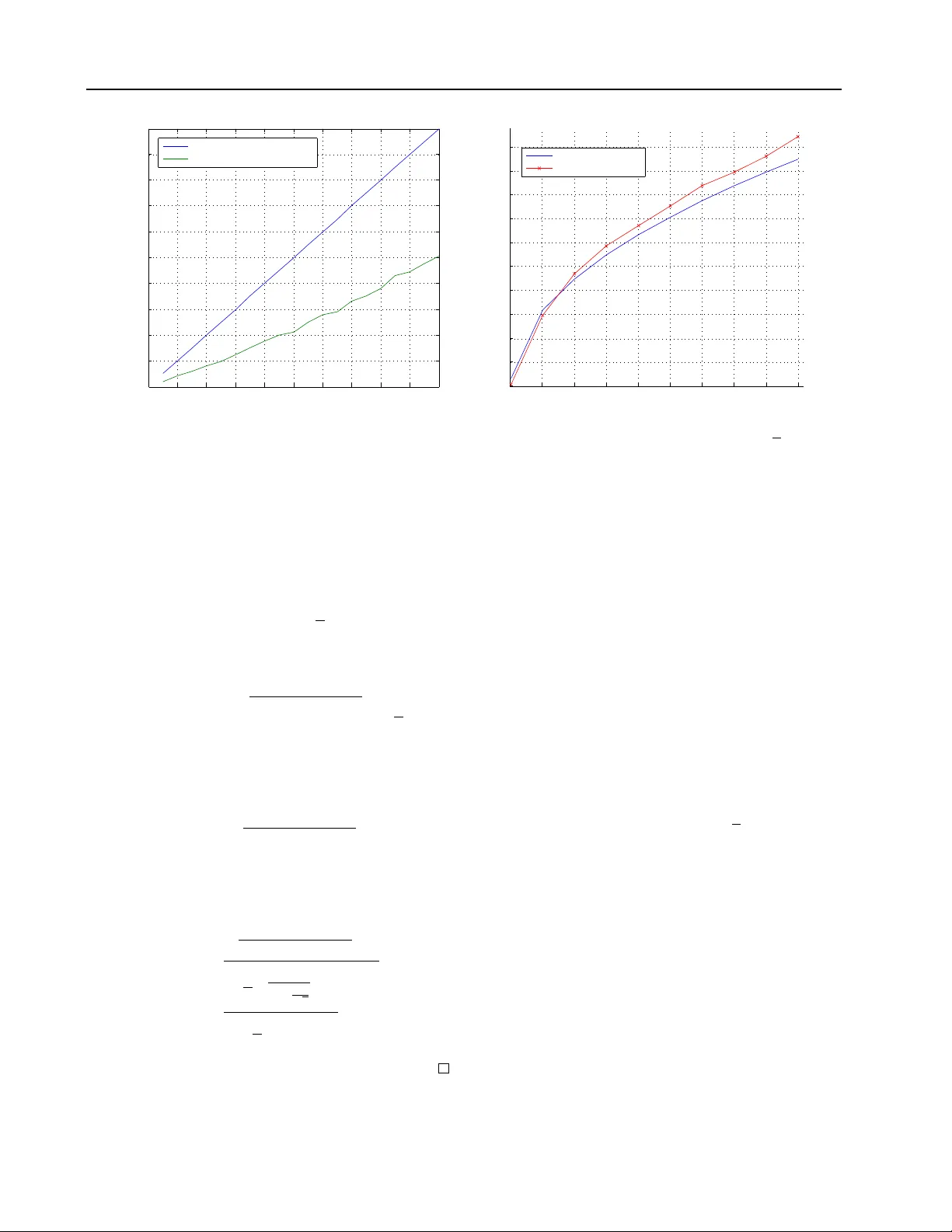
Rapid Learning with Sto c hastic F o cus of A tten tion Raphael P elossof pelossof@cbio.mskcc.or g Comp. Bio. Sloan Kettering Zhiliang Ying zying@st a t.columbia.edu Statistics Departmen t Columbia Univ ersity Abstract W e presen t a metho d to stop the ev aluation of a decision making pro cess when the re- sult of the full ev aluation is ob vious. This trait is highly desirable for online margin- based machine learning algorithms where a classifier traditionally ev aluates all the fea- tures for every example. W e observe that some examples are easier to classify than oth- ers, a phenomenon whic h is c haracterized b y the even t when most of the features agree on the class of an example. By stopping the feature ev aluation when encoun tering an easy to classify example, the learning algo- rithm can ac hieve substantial gains in com- putation. Our method pro vides a natural at- ten tion mechanism for learning algorithms. By mo difying P egasos, a margin-based online learning algorithm, to include our attentiv e metho d w e low er the num b er of attributes computed from n to an av erage of O ( √ n ) features without loss in prediction accuracy . W e demonstrate the effectiveness of Atten- tiv e Pegasos on MNIST data. 1. In tro duction The running time of margin based online algorithms is a function of the n umber of features, or the dimension- alit y of the input space. Since mo dels to da y may ha ve thousands of features, running time seems daun ting, and dep ending on the task, one may wish to sp eed- up these online algorithms, by pruning uninformativ e examples. W e propose to early stop the computation of feature ev aluations for uninformative examples by connecting Sequen tial Analysis ( W ald , 1945 ; Lan et al. , App earing in Pr o c e e dings of the 28 th International Con- fer enc e on Machine L e arning , Bellevue, W A, USA, 2011. Cop yright 2011 b y the author(s)/owner(s). 1982 ) to margin based learning algorithms. Man y decision making algorithms mak e a decision by comparing a sum of observ ations to a threshold. If the sum is smaller than a pre-defined threshold a certain action is taken, otherwise a differen t action is taken or no action is taken. This type of reasoning is prev a- len t in the margin-based Mac hine Learning commu- nit y , where typically an additiv e mo del is compared to a threshold, and a subsequent action is tak en dep end- ing on the result of the comparison. Margin-based learning algorithms a verage multip le weak hypotheses to form one strong com bined h yp othesis - the ma jor- it y vote. When training, the combined hypothesis is usually compared to a threshold to make a decision ab out when to up date the algorithm. When testing, the combined hypothesis is compared to a threshold to mak e a predictive decision ab out the class of the ev aluated example. With the rapid growth of the size of data sets, b oth in terms of the num b er of samples, and in terms of the dimensionalit y , margin based learning algorithms can av erage thousands of hypotheses to create a single highly accurate combined hypothesis. Ev aluating all the h yp otheses for eac h example becomes a daun ting task since the size of the data set can b e very large, in terms of n umber of examples and the dimensionalit y of eac h example. In terms of num b er of examples, we can sp eed up pro cessing b y filtering out un-informative ex- amples for the learning pro cess from the data set. The measure of the imp ortance of an example is typically a function of the ma jority vote. In terms of dimen- sionalit y , we w ould lik e to compute the least num b er of dimensions b efore w e decide whether the ma jority v ote will end b elow or ab ov e the decision threshold. Filtering out un-informative examples, and trying to compute as few hypotheses as p ossible are close ly re- lated problems ( Blum & Langley , 1997 ). The decision whether an exam ple is informativ e or not dep ends on the magnitude of the m a jorit y rule, that is the amount A ttentiv e Learning and Prediction of disagreemen t b et ween the hypotheses. Therefore, to find whic h example to filter, the algorithm needs to ev aluate its ma jorit y vote, and we would like it to ev aluate the least num b er of weak hypotheses b efore coming to a decision ab out the example’s imp ortance. Ma jority v ote based decision making can b e general- ized to comparing a weigh ted sum of random v ariables to a giv en threshold. If the ma jorit y vote falls b elo w the pre-specified threshold a decision is made, typi- cally the mo del is up dated, otherwise the example is ignored. Since, the ma jority vote is a summation of w eighted random v ariables, or av eraged w eak hypothe- ses, it can b e computed sequentially . Sequential Anal- ysis allows us to dev elop the statistical needed to sp eed up this ev aluation pro cess when its result is evident. W e use the terms margin and full margin to describ e the summation of all the feature ev aluations, and par- tial margin as the summation of a part of the feature ev aluations. The calculation of the margin is broken up for each example in the stream. This break-up allo ws the algorithm to make a decision after the ev al- uation of each feature whether the next feature should also be ev aluated or the feature ev aluation should be stopp ed, and the example should be rejected for lac k of imp ortance in training. By making a decision after eac h ev aluation w e are able to early stop the ev aluation of features on examples with a large partial margin af- ter having ev aluated only a few features. Examples with a large partial margin are unlikely to hav e a full margin b elo w the required threshold. Therefore, by rejecting these examples early , large savings in com- putation are ac hieved. This pap er prop oses sev eral simple nov el metho ds based on Sequential Analysis ( W ald , 1945 ; Lan et al. , 1982 ) and stopping metho ds for Brownian Motion to drastically impro ve the computational efficiency of margin based learning algorithms. Our metho ds ac- curately stop the ev aluation of the margin when the result is the en tire summation is evident. Instead of lo oking at the traditional classification er- ror we lo ok at decision error. Decision errors are er- rors that o ccur when the algorithm rejects an example that should be accepted for training. Given a desired decision error rate we would lik e the test to decide when to stop the computation. This test is adap- tiv e, and changes according to the partial computa- tion of the margin. W e demonstrate that this simple test can sp eed-up Pegasos by an order of magnitude while main taining generalization accuracy . Our no v el algorithm can b e easily parallelized. 2. Related W ork Margin based learning has spurred countless algo- rithms in man y different disciplines and domains. T ypically a margin based learning algorithm ev aluates the sign of the margin of eac h example and p erforms a decision. Our work provides early stopping rules for the margin ev aluation when the result of the full ev al- uation is obvious. This approach low ers the a verage n umber of features ev aluated for each example accord- ing to its importance. Our stopping thresholds apply to the ma jority of margin based learning algorithms. The most directly applicable machine learning algo- rithms are margin based online learning algorithms. Man y margin based Online Algorithms base their mo del up date on the margin of each example in the stream. Online algorithms such as Kivinen and W ar- m uth’s Exponentiated Gradient ( Kivinen & W armuth , 1997 ) and Oza and Russell’s Online Bo osting ( Oza & Russell , 2001 ) up date their respective mo dels b y using a margin based p oten tial function. P assive online algo- rithms, such as Rosen blatt’s p erceptron ( Rosenblatt , 1958 ) and Crammer etal’s online passiv e-aggressive algorithms ( Crammer et al. , 2006 ), define a margin based filtering criterion for up date, whic h only up- dates the algorithm’s mo del if the v alue of the mar- gin falls b elo w a defined threshold. All these algo- rithms fully ev aluate the margin for each example, whic h means that they ev aluate all their features for ev ery example. Recen tly Shalev-Shw artz & Srebro ( 2008 ); Shalev-sh wartz et al. ( 2010 ) prop osed P ega- sos, an online stochastic gradien t descen t based SVM solv er. The solver is a sto c hastic gradient descent solv er which pro duces a maximum margin classifier at the end of the training pro cess. The abov e men tioned algorithms passiv ely ev aluate all the features for each giv en example in the stream. Ho wev er, if there is a cost (such as time) assigned to a feature ev aluation we would like to design an efficient learner whic h activ ely c hoose which features it would lik e to ev aluate. Similar work on the idea of learning with a feature budget w as first introduced to the ma- c hine learning communit y in Ben-David & Dic hterman ( 1998 ). The authors introduced a formal framew ork for the analysis of learning algorithm with restrictions on the amoun t of information they can extract. Sp ecif- ically allo wing the learner to access a fixed amount of attributes, which is smaller than the en tire set of at- tributes. They presen ted a framew ork that is a natural refinemen t of the P AC learning mo del, how ever tradi- tional P AC c haracteristics do not hold in this frame- w ork. V ery recently , b oth Cesa-Bianchi et al. ( 2010 ) and Reyzin ( 2010 ) studied how to efficiently learn a A ttentiv e Learning and Prediction !"# $"%&#'() *+"(,-")!"# $"%&#'() .(/'#01,-")" 210%3") 4(5(/'#01,-")" 210%3") 6- 1371&"8)/ "1&7#") 9'& :"-1371&"8)/ "1&7#") ;78<"&"8)! "#$"%&#'() ="1&7#")" -1371,'() Figure 1. Two examples are classified. The first is hard to classify , the second easy . The budgeted learning approach w ould ev aluate the same num b er of features for both examples, whereas the sto c hastic would ev aluate features according to how hard is the example to classify , while main taining an av erage budget. linear predictor under a feature budget (see figure 1 .) Also, ( Clarkson et al. , 2010 ) extended the Perceptron algorithm to efficiently learn a classifier in sub-linear time. Similar active learning algorithms were developed in the con text of when to pa y for a label (as opp osed to an attribute). Such activ e learning algorithms are presen ted with a set of unlabeled examples and de- cide whic h examples lab els to query at a cost. The algorithm’s task is to pay for lab els as little as p os- sible while ac hieving sp ecified accuracy and reliability rates ( Dasgupta et al. , 2005 ; Cesa-Bianc hi et al. , 2006 ). T ypically , for selective sampling activ e learning algo- rithms the algorithm w ould ignore examples that are easy to classify , and pa y for lab els for harder to classify examples that are close to the decision b oundary . Our work stems from connecting the underlying ideas b et w een these tw o active learning domains, attribute querying and lab el querying. The main idea is that t ypically an algorithm should not query man y at- tributes for examples that are easy to classify . The lab els for such examples, in the lab el query active learning setting, are typically not queried. F or suc h examples most of the attributes w ould agree to the classification of the example, and therefore the algo- rithm need not ev aluate to o man y before deciding the imp ortance of such examples. 3. The Sequen tial Thresholded Sum T est The no v el Constant Se quential Thr esholde d Sum T est is a test which is designed to con trol the rate of deci- sion errors a margin based learning algorithm mak es. Although the test is known in statistics, it hav e never b een applied to learning algorithms b efore. 3.1. Mathematical Roadmap Our task is to find a filtering framew ork that would sp eed-up margin-based learning algorithms by quic kly rejecting examples of little imp ortance. Quic k rejec- tion is done by creating a test that stops the margin ev aluation process giv en the partial computation of the margin. W e measure the importance of an example b y the size of its margin. W e define θ as the imp or- tance threshold, where examples that are important to learning hav e a margin smaller than θ . Statistically , this problem can b e generalized to finding a tes t for early stopping the computation of a partial sum of in- dep enden t random v ariables when the result of the full summation is guaran teed with a high probability . W e lo ok at decision errors of a sum of weigh ted in- dep enden t random v ariables. Then given a required decision error rate w e will deriv e the Constant Se quen- tial Thr esholde d Sum T est (Constant STST) whic h will pro vide adaptive early stopping thresholds that main- tain the required confidence. Let the sum of w eighted independent random v ariables ( w i , X i ) , i = 1 , ..., n b e defined b y S n = P n i =1 w i X i , where w i is the weigh t assigned to the random v ari- able X i . W e require that w i ∈ R, X i ∈ [ − 1 , 1]. W e define S n as the full sum, S i as the partial sum, and S in = S n − S i = P n j = i +1 w i X i as the remaining sum. Once w e computed the partial sum up to the i th ran- dom v ariable w e know its v alue S i . Let the stopping threshold at co ordinate i b e defined b y τ i . W e use the notation E S in to denote the exp ected v alue the remaining sum. There are four basic ev ents that we are interested in when designing sequential tests whic h inv olve control- ling decision error rates. Each of these even ts is impor- tan t for differen t applications under different assump- tions. The sequential metho d lo oks at ev en ts that in- v olve the en tire random walks, whereas the curtailed metho d lo oks at evens that accumulate information A ttentiv e Learning and Prediction as the random walk progresses. Let us establish the basic relationship betw een the sequential method, on the left hand side of the following equations, and the curtailed metho d on the right hand side: P ( stop | S n < θ ) P ( S n < θ ) = P ( S n < θ | stop ) P ( stop ) , (1) where stop is the even t which o ccurs when the partial sum crosses a stopping boundary stop . = { S i > τ i } . Previously ( ? ) a Curved STST was prop osed by lo ok- ing at the follo wing “curtailed” conditional probabilit y P ( S n < θ | stop ) = P ( S n < θ , stop ) P ( stop ) . (2) The simplicity of deriving the curtailed metho d stems from the fact that the join t probabilit y and the stop- ping time probabilit y are not needed to b e explic- itly calculated to upp er b ound this conditional. The resulting first stopping b oundary , the curv ed b ound- ary , gives us a constant conditional error probabilit y throughout the curve, which meant that it is a rather conserv ativ e b oundary . W e develop a more aggressiv e boundary whic h allows higher decision error rates at the b eginning of the ran- dom walk and low er decision error rates at the end. Suc h a b oundary would essentially stop more random w alks early on, and less later later on. This approach has the natural interpretation that w e wan t to shorten the feature ev aluation for ob vious un-important sam- ples, but we wan t to prolong the ev aluations for sam- ples we are not sure ab out. A Constan t b oundary ac hieves this exact “error sp ending” characteristic. 3.2. The Constan t Sequential Thresholded Sum T est W e condition the probability of making a decision error in the follo wing wa y P (stop b efore n | S n < θ ) = P (stop b efore n, S n < θ ) P ( S n < θ ) . (3) W e stated in equation 3 a conditional probabilit y func- tion which is conditioned on the examples of in terest. Therefore in this case we are in terested in limiting the decision error rate for examples that are imp ortan t. T o upp er b ound this conditional we will make an approx- imation that will allow us to apply b oundary-crossing inequalities for a Bro wnian bridge. T o apply the Brow- nian bridge to our conditional probabilit y we appro x- imate it b y P (stopp ed b efore n | S n < θ ) (4) = P (max i S i > τ | S n < θ ) (5) ≈ P (max i S i > τ | S n = θ ) . (6) If w e assume that the even t { S n < θ } is rare (equiv- alen tly that E X i > 0), then w e can approximate the inequalit y with an equalit y , which gives a Brownian bridge. Now w e need to calculate b oundary crossing probabilities of the Bro wnian bridge and a constant threshold. Lemma 1. The Br ownian bridge Stopping Boundary. L et T τ = inf { i : S i = τ } b e the first hitting time of the r andom walk and c onstant τ . Then the pr ob ability of the fol lowing de cision err or is P ( T τ < n | S n = θ ) = e − 2 τ ( τ − θ ) var ( S n ) . Pr o of. See App endix. Theorem 1. The Simplifie d Contant STST b oundary ( θ = 0 ), τ = p v ar ( S n ) q log 1 √ δ makes appr oximately δ de cision mistakes { T τ < n | S n < 0 } . Pr o of. By approximating P ( S i > τ | S n < θ ) ≈ P ( S i > τ | S n = θ ) and setting this probability to δ we get the Con tant STST b oundary P ( S i > τ | S n < θ ) ≈ exp  − 2 τ ( τ − θ ) v ar ( S n )  = δ. (7) Solving, τ 2 − τ θ = v ar ( S n ) log 1 √ δ (8) ( τ − θ ) 2 − 1 4 θ 2 = v ar ( S n ) log 1 √ δ (9) τ = θ + s 1 4 θ 2 + v ar ( S n ) log 1 √ δ . (10) If w e simplify this b oundary by setting θ to zero, w e get the theorem’s b oundary τ = p v ar ( S n ) s log 1 √ δ . There are t wo appealing things ab out this boundary , the first that it’s not dep enden t on E S i , and that it is alw ays positive. Secondly , when using this b oundary for prediction, we can directly see the implication on the error rate of the classifier, since the decision error essen tially b ecomes a classification error, a fact that is also clearly eviden t throughout the exp erimen ts. A ttentiv e Learning and Prediction 0 0.02 0.04 0.06 0.08 0.1 0.12 0.14 0.16 0.18 0.2 0 0.02 0.04 0.06 0.08 0.1 0.12 0.14 0.16 0.18 0.2 Decision error rate for the Brownian bridge boundary delta delta Wanted error rate δ Actual Brownian bridge error rate (a) A sim ulation of the Bro wnian bridge boundary with X i ∼ N (0 . 05 , 1). The b oundary is conserv ative. 0 1000 2000 3000 4000 5000 6000 7000 8000 9000 0 200 400 600 800 1000 1200 1400 1600 1800 2000 number of features n Expected stopping time t Expected and actual stopping times for the Brownian bridge boundary Expected stopping time Actual stopping time (b) The boundary behav es similarly to what’s expected from theory . It computes in the order of O ( √ n ) fea- tures. Figure 2. Performance of the Brownian bridge b oundary . 3.3. Av erage Stopping Time for the Curved and Constan t STST W e are able to show that the exp ected num b er of fea- tures ev aluated for the Curv ed and the Constan t STST b oundaries is in the order of O ( √ n ). This can be ob- tained b y limiting the range of v alues X i can tak e. Theorem 2. L et | X i | ≤ k , and let E X i > 0 . L et the stopping time of the Br ownian bridge b e define d by t = inf { i : S i ≥ p v ar ( S n ) log δ − 0 . 5 } . Then the exp e cte d stopping time is in the or der of O ( √ n ) . Pr o of. E S T = E S T − 1 + E X T (11) ≤ E S T − 1 + k (12) ≤ p v ar ( S n ) log δ − 0 . 5 + k (13) The second inequality holds since the random w alk only crossed the b oundary for the first time at time T and therefore w as under the boundary at time T − 1. By applying W ald’s Equation E S T = E T E X w e get E T = p v ar ( S n ) log δ − 0 . 5 + k E X (14) ≤ c √ n q log 1 √ δ + k E X (15) = O ( √ n ) , (16) where c, k , and E X are constan ts. See figure 2(a) for simulation results. 4. A ttentiv e Pegasos P egasos by ( Shalev-shw artz et al. , 2010 ) is a simple and effective iterative algorithm for solving the opti- mization problem cast b y Supp ort V ector Machines. T o solve the SVM functional it alternates b et ween sto c hastic gradient descent steps (weigh t up date) and pro jection steps (weigh t scaling). Similarly to the P erceptron these steps are tak en when the algorithm mak es a classification error while training. F or a lin- ear kernel, the total run-time of Pegasos is ˜ O ( d/ ( λ )), where d is the num b er of non-zero features in each ex- ample, λ is a regularization parameter, and  is the error rate incurred by the algorithm o ver the optimal error rate ac hiev able. By assuming that the features are independent, and applying the Brownian bridge STST we sp eed up Pegasos to ˜ O ( √ d/ ( λ )) without losing significant accuracy . The algorithm Attentive Pe gasos is demonstrated in Algorithm 1 . 4.1. Exp erimen ts W e conducted sev eral exp erimen ts to test the sp eed, generalization capabilities, and predictiv e accuracy of the STST. W e ran Pegasos, Atten tiv e P egasos and Budgeted Pegasos on 1-vs-1 MNIST digit classification tasks. W e also tested different sampling and ordering metho ds for co ordinate selection. A ttentiv e Pegasos stops the computation of examples that were unlikely to hav e a negative margin early . W e computed the a verage n um b er of features the algo- A ttentiv e Learning and Prediction Algorithm 1 Atten tive P egasos Input : D ataset { X l , y l } m l =1 , λ, δ Initialize : Cho ose w 1 s.t. || w 1 || ≤ 1 / √ λ, j = 0 for l = 1 , 2 , ..., m do if ∃ i = 1 , .., n s.t. y l P i j =1 w i x l i ≥ 1 + q P n j =1 w j · v ar y l ( x j ) p log δ − 0 . 5 then Up date v ar y l ( x j ) , j = 1 , .., i w l = w l − 1 Jump to next example else Set µ l = 1 lλ Set w l + 1 2 = (1 − µ l λ ) w l + µ l y x Set w l +1 = min  1 , 1 / √ λ || w l + 1 2 ||  end if end for return w m +1 rithm computed for examples that were filtered, and compare it to a budgeted version of Pegasos, where only a fixed n umber of features are ev aluated for an y example. W e ran 1-vs-1 digit classification problems under differen t feature selection p olicies. With the first p olicy , we sorted the co ordinates, such that coordi- nates with a large absolute weigh t b efore other features with lesser absolute weigh t. Then with the second, we ran exp erimen ts where the co ordinates w ere selected b y sampling from the weigh t distribution with replace- men t. Finally , with the third, we ran exp eriments where the co ordinates were randomly p erm uted. F or each one of these scenarios, three algorithms were run 10 times on different p erm utations of the datasets and their results were av eraged (Figure 4 .) W e first ran A ttentiv e P egasus under eac h of the coordinate selection metho ds. Then we set the budget for Bud- geted Pegasus as the a verage num b er of features that w e got through Atten tive P egasos. Finally , we ran the full Pegasus with a trivial b oundary , which essentially computes everything. Both figures sho w that using the Bro wnian Bridge b oundary can sav e in the order of 10x computation, and maintain similar generalization re- sults to the full computation. Also, sorting under the Budgeted Pegasos is imp ossible since we need to learn the w eights in order to sort them. Therefore we did not run Budgeted P egasos with sorted weigh ts. W e can see in the middle subfigure, that the A ttentiv e, Bud- geted, and F ull algorithms maintain almost identical generalization results. How ev er, when we early stop prediction with the resulting mo del, Atten tive Pega- sos giv es the b est predictive results, ev en better than what we get with the full computation but only com- putes a ten th of the feature v alues! 4.2. Conclusions W e sp ed up online learning algorithms up to an order of magnitude without any significan t loss in predictive accuracy . Surprisingly , in prediction A tten tive P egasos outp erformed the original Pegasus, ev en though it. In addition, we prov ed that the exp ected sp eedup under indep endence assumptions of the weak h yp otheses is O ( √ n ) where n is the set of all features used by the learner for discrimination. The thresholding pro cess creates a natural attention mec hanism for online learning algorithms. Examples that are easy to classify (such as bac kground) are fil- tered quickly without ev aluating many of their fea- tures. F or examples that are hard to classify , the ma- jorit y of their features are ev aluated. By sp ending lit- tle computation on easy examples and a lot of com- putation on hard “interesting” examples the Atten- tiv e algorithms exhibit a sto chastic fo cus-of-atten tion mec hanism. It would b e interesting to find an explanation for our results where the attentiv e algorithm outp erforms the full computation algorithm in the prediction task. 5. App endix Lemma 2. Br ownian bridge b oundary cr ossing pr ob- ability P ( T τ < n | S n = θ ) = exp  − 2 τ ( τ − θ ) v ar ( S n )  . (17) Pr o of. W e can lo ok at an infinitesimally small area dθ around θ P ( T τ ≤ n | S n = θ ) = P ( T τ < n, S n = θ ) P ( S n = θ ) . (18) The n umerator can b e developed to P ( T τ < n, S n = θ ) (19) = P ( T τ < n ) P ( S n ∈ dθ | T τ < n ) (20) = P ( T τ < n ) P ( S n ∈ 2 τ − dθ | T τ < n ) (21) = P ( S n ∈ 2 τ − dθ , T τ < n ) (22) = P ( S n ∈ 2 τ − dθ ) (23) = 1 p v ar ( S n ) φ 2 τ − θ p v ar ( S n ) ! dθ (24) Similarly , the denominator denominator = 1 p v ar ( S n ) φ θ p v ar ( S n ) ! dθ A ttentiv e Learning and Prediction sort sample rand 0 100 200 300 400 500 600 700 800 49 363 193 193 710 276 277 730 Computation sort sample rand 0 0.5 1 1.5 2 2.5 3 3.5 2.92% 2.91% 2.73% 3.18% 2.82% 2.91% 3.02% 3.17% Test error % sort sample rand 0 1 2 3 4 5 6 2.48% 2.91% 3.61% 5.53% 3.71% 2.51% 5.76% 3.17% Prediction error % bbBoundary budgetedBoundary noBoundary Figure 3. Results for A ttentiv e P egasos, MNIST 2 vs 3, δ = 10%. Our Brownian bridge decision boundary (blue) pro cesses only 49 feature on a verage (15 times faster than full computation), while achieving similar generalization as the fully trained classifier (red, middle subfigure). On the righ t subfigure, when the b oundary is applied to prediction, Atten tive P egasus ac hieves a lo wer error rate than the full computation, and less than half the error of the Budgeted Boundary (green). Plugging bac k into 18 P ( T τ < n | S n = θ ) (25) = φ  2 τ − θ √ v ar ( S n )  φ  θ √ v ar ( S n )  (26) = exp  − 1 2 (2 τ − θ ) 2 v ar ( S n ) + 1 2 θ 2 v ar ( S n )  (27) = exp  − 2 τ ( τ − θ ) v ar ( S n )  . (28) Definition 1. A r andom variable T which is a func- tion of X 1 , X 2 , ... is a stopping time if T has none gative inte ger values and for al l n = 1 , 2 , ... ther e is an event A n such that T ≤ n if and only if ( X 1 , ..., X n ) ∈ A n , while for n = 0 , { T = 0 } is either empty (the usual c ase) or the whole sp ac e. F or a nonne gative inte ger- value d r andom variable X , we have ∞ X j =1 P ( X ≥ j ) (29) = ∞ X j =1 X k ≥ j P ( X = k ) = ∞ X k =1 P ( X = k ) k X j =1 1 = ∞ X k =1 k P ( X = k ) = E X ≤ + ∞ (30) Lemma 3. (( Wald , 1945 ), pr o of fr om ( ? )) W ald’s Iden tity . L et S T b e a sum of indep endent identi- c al ly distribute d r andom variables X 1 + ... + X T , wher e E X i < ∞ . L et S n = X 1 + ... + X n , i > T and S 0 = 0 . L et T = { inf i S i = a } , T > 0 wher e a is a c onstant b e a r andom variable with E T < ∞ . Then E S T = E T E X . Pr o of. If T = 0 the identit y is trivial. Otherwise E S T = ∞ X n =1 P ( T = n ) E ( X 1 + ... + X n | T = n ) (31) = ∞ X n =1 P ( T = n ) n X j =1 E ( X j | T = n ) (32) = ∞ X j =1 ∞ X n = j P ( T = n ) E ( X j | T = n ) (33) = ∞ X j =1 ∞ X n = j E ( X j 1 T = n ) (34) = ∞ X j =1 E ( X j 1 T ≥ j ) (35) = ∞ X j =1 E ( X j (1 − 1 T ≤ j − 1 ) . (36) The even t { T ≤ j − 1 } is indep enden t of Y j , therefore E S T = ∞ X j =1 E ( X j ) P ( T ≥ j ) (37) = E X ∞ X j =1 P ( T ≥ j ) = E X E T (38) A ttentiv e Learning and Prediction sort sample rand 0 100 200 300 400 500 600 700 800 72 363 196 197 720 279 279 735 Computation sort sample rand 0 0.5 1 1.5 2 2.5 2.01% 1.77% 1.77% 2.21% 2.06% 2.11% 2.16% 1.87% Test error % sort sample rand 0 0.5 1 1.5 2 2.5 3 3.5 1.06% 1.77% 2.23% 3.27% 2.71% 1.70% 3.14% 1.87% Prediction error % bbBoundary budgetedBoundary noBoundary Figure 4. Results for A ttentiv e Pegasos. MNIST 3 vs 10, δ = 10%. Our Brownian bridge decision b oundary (blue) pro cesses only 72 feature on av erage, while achieving similar generalization as the fully trained classifier. On the right, when the b oundary is applied to classification, Atten tive Pegasus gets a low er error rate than the full computation, and o ver a 2% adv an tage ov er the Budgeted Boundary . b y definition 1 . References Ben-Da vid, Shai and Dich terman, Eli. Learning with restricted fo cus of attention. Journal of Computer and System Scienc es , 56(3):277 – 298, 1998. Blum, Avrim L. and Langley , Pat. Selection of relev ant features and examples in machine learning. Artificial intel ligenc e , 97(1-2):245–271, 1997. Cesa-Bianc hi, Nicolo, Gentile, Claudio, and Zanib oni, Luca. W orst-case analysis of selectiv e sampling for linear classification. Journal of Machine L e arning R ese ar ch , 7:1205–1230, 2006. ISSN 1533-7928. Cesa-Bianc hi, Nicolo, Shalev-Sh wartz, Shai, and Shamir, Ohad. Efficient learning with partially ob- serv ed attributes. In International Confer enc e on Machine L e arning , 2010. Clarkson, Kenneth L., Hazan, Elad, and W oo druff, Da vid P . Sublinear optimization for machine learn- ing. F oundations of Computer Scienc e, Annual IEEE Symp osium on , 0:449–457, 2010. ISSN 0272- 5428. doi: http://doi.ieeecomputersociety .org/10. 1109/F OCS.2010.50. Crammer, Koby Crammer, Dekel, Ofer, Keshet, Joseph, and Singer, Y oram. Online passiv e- aggressiv e algorithms. Journal of Machine L e arning R ese ar ch , 7:551–585, 2006. Dasgupta, Sanjoy , Kalai, Adam T auman, and Mon- teleoni, Claire. Analysis of perce ptron-based activ e learning. In In COL T , pp. 249–263, 2005. Kivinen, Jyrki and W arm uth, Manfred K. Exp onen ti- ated gradient versus gradient descent for linear pre- dictors. Information and Computation , 132(1):1–63, 1997. ISSN 0890-5401. doi: h ttp://dx.doi.org/10. 1006/inco.1996.2612. Lan, K.K. Gordon, Simon, Richard, and Halp erin, Max. Sto c hastically curtailed tests in long-term clin- ical trials. Se quential Analysis , 1(3):207–219, 1982. Oza, N. and Russell, S. Online bagging and b oost- ing. In Artificial Intel ligenc e and Statistics , pp. 105– 112. Morgan Kaufmann, 2001. URL citeseer.ist. psu.edu/oza01online.html . Reyzin, Lev. Bo osting on a feature budget. In Interna- tional Confer enc e on Machine L e arning, Budgete d L e arning workshop , 2010. Rosen blatt, F. The p erceptron: A probabilistic mo del for information storage and organization in the brain. Psycholo gic al R eview , 65(6):386–408, 1958. Shalev-Sh wartz, Shai and Srebro, Nathan. Svm opti- mization: inv erse dep endence on training set size. In International Confer enc e on Machine L e arning , pp. 928–935. A CM, 2008. Shalev-sh wartz, Shai, Singer, Y oram, Srebro, Nathan, and Cotter, Andrew. P egasos: Pri- mal estimated sub-gradien t. 2010. URL A ttentiv e Learning and Prediction http://citeseerx.ist.psu.edu/viewdoc/ summary?doi=10.1.1.161.9629 . W ald, A. Sequen tial tests of statistical hypotheses. The Annals of Mathematic al Statistics , 16(2):117– 186, 1945. ISSN 00034851. URL http://www. jstor.org/stable/2235829 .