Learning Active Basis Models by EM-Type Algorithms

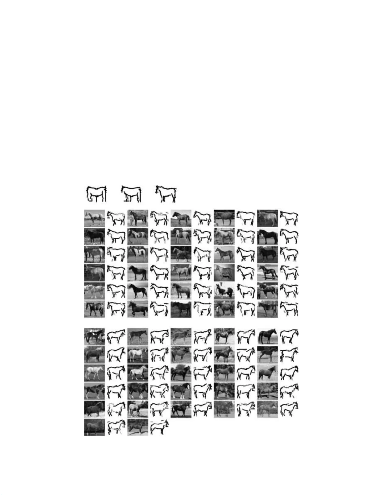
Statistic al Scienc e 2010, V ol. 25, No. 4, 458– 475 DOI: 10.1214 /09-STS281 c  Institute of Mathematical Statisti cs , 2010 Lea rning Active Basis Mo dels b y EM-T yp e Algo rithms Zhangzhang Si , Hai feng Go ng , Song-Chun Zhu and Ying Nian W u Abstr act. EM algorithm is a con ve nient to ol for maximum lik eliho o d mo del fitting when the data are incomplete or w h en there are laten t v ariables or hid den states. In this review article we explain that EM algorithm is a natural compu tational scheme for learning im age tem- plates of ob ject catego ries where the learning is not f u lly su p ervised. W e represent an image template b y an activ e basis mo del, whic h is a linear comp osition of a selected set of localized, elo ngated and oriente d w a v elet elemen ts that are allo we d to slightly p ertur b their lo cations and orientat ions to accoun t for the d eformations of ob ject sh ap es. The mo del can b e easily learned when the ob jects in the training images are of the same p ose, and app ear at the same location and scale. T h is is often called sup e rvised learning. In the situation wh ere the ob jects ma y app ear at differen t unknown locations, orien tations and scales in the training images, we ha v e to incorp orate the unkn o wn lo cations, orien tations and scales as latent v ariables into the image generatio n pro cess, and learn the template by EM-type algorithms. The E -step im- putes the u nknown lo cations, orien tations and scales based o n th e cur- ren tly learned template. T h is step can b e considered self-sup ervision, whic h inv olve s using the current template to r ecognize the ob jects in the training images. Th e M-step then relearns the template b ased on the impu ted lo cations, orien tations and scales, and this is essential ly the same as sup ervised learning. So the EM learning pro cess iterates b et wee n reco gnition and sup ervised learnin g. W e illustrate th is sc heme b y sev eral exp eriments. Key wor ds and phr ases: Generativ e mo dels, ob ject r ecognition, wa vel et sparse cod ing. Zhangzhang Si is Ph.D. Student, Dep artment of Statistics, University o f California, L os Angel es, USA e-mail: zzsi@stat.ucla.e du . Haifeng Gong is Postdo ctor al R ese ar cher, Dep artment of Statistics, University of Califo rnia, L os A ngeles, USA and L otu s Hil l R ese ar ch Institute, Ezhou, China e-mail: hfgong@stat.ucla.e du . Song-Chun Zhu is Pr ofessor, Dep artment of St atistics, University of C alifornia, L os Angeles, USA and L otus Hil l R ese ar ch Institute, E zhou, China e-mail: sczhu@stat.ucla.e du . Ying Nian Wu is Pr ofessor, Dep artment of Statistics, University of Califo rnia, L os Angele s, USA e-mail: y wu@st at.ucla.e du . 1. INTRODUCTION: EM LEARNING S CHEME The EM alg orithm [ 7 ] and its v ariations [ 14 ] hav e b een widely used for maxim um lik eliho o d estimation of statistical mo dels when the data are incompletely observ ed or when there are laten t v ariables or hid- den states. This algorithm is an iterativ e computa- tional scheme, where the E-step imputes the miss- ing data or the laten t v ariables giv en the curren tly This is a n electronic r eprint o f the original article published by the Institute of Ma thema tical Statistics in Statistic al Scienc e , 2010, V ol. 25, No. 4, 458–47 5 . This reprint differ s from th e original in paginatio n and t yp ogr aphic detail. 1 2 SI, GON G, ZH U A N D WU estimated mo d el, and the M-step re-esti mates the mo del giv en the impu ted missing data or laten t v ari- ables. Be sides its simplicit y and stabilit y , a key fea- ture that distinguishes th e EM algorithm f rom other n umerical metho ds is its inte rpr etabilit y: b oth the E-step and the M-step readily admit natural inter- pretations in a v ariety of con texts. This makes the EM alg orithm ric h, m eanin gfu l and inspiring. In this review article w e shall fo cus on one imp or- tan t context w here the EM algorithm is useful and meaningful, that is, learning patterns from signals in the sett ings that are not fully sup ervised. In t his con text, th e E -step can b e inte rpr eted as carrying out th e recognition task u s ing the c urr en tly le arned mo del of the pattern. The M-step can b e inte rpr eted as relearning the p attern in the sup ervised setting, whic h can often b e easily acco mplished. This EM learnin g scheme has b een used in b oth sp eec h and vision. In sp eec h recognition, the train- ing of the hidden Marko v mo del [ 16 ] inv olves the imputation of th e hid den states in the E-step by the forwa rd and backw ard algorithms. The M-step computes the tran s ition and emission fr equ encies. In computer vision, we w an t to learn mod els for differ- en t categories of ob jects, such as horses, bird s, bik es, etc. The learning is ofte n easy when th e ob jects in the training images are aligned, in the s ense that the ob jects a pp ear at the same p ose, same location and same scale in the training images, which are defi ned on a common image lattice that is the b ound ing b ox of th e ob jects. T his is often called sup er v ised le arn- ing. How ev er, it is often the case that the ob jects app ear at differen t unkn o wn lo cations, orien tations and scales in the training images. In suc h a situa- tion, w e h a v e to incorp orate the un k n o wn lo cations, orien tations and scales as laten t v ariables in the im- age generation pro cess, and u se the EM algorithm to learn t he mo del for the ob jects. In the EM learning pro cess, the E -step impu tes the unknown lo cation, orien tation and scale of the ob ject in eac h training image, based on the currently learned m o del. Th is step uses the current mo del to recognize the ob ject in eac h training image, that is, wh er e it is, at what orien tation and scale. The imputation of the laten t v ariables enables us to al ign the training images, so that the ob jects app ear at the same location, ori- en tation and scale. The M-step then relearns the mo del from the alig ned images b y carrying out su- p ervised learning. S o the EM learning pro cess it- erates betw een recog nition and su p ervised learning. Recognitio n is the goal of learnin g the mo del, and it serve s as the self-sup ervision step of the learnin g pro cess. The EM algorithm has b een used b y F ergus, P erona and Zisserman [ 9 ] in training the constella- tion mo del for ob jects. In this article we sh all illus tr ate EM learning or EM-lik e learnin g by training an activ e basis mo del [ 22 , 23 ] that w e ha v e recen tly d ev elop ed for deformable templates [ 1 , 24 ] of ob ject shap es. In this mo d el, a template is repr esen ted by a linear comp osition o f a set of localized, elonga ted and orien ted w av elet ele- men ts at se lected lo cations, scales and o rienta tions, and these w a v elet elemen ts are allo wed to sligh tly p ertur b their lo cations and orien tations to accoun t for the shap e deformations of the ob jects. In the sup ervised setting, the activ e b asis mo del can b e learned b y a shared ske tc h algorithm, whic h selects the w a v elet elemen ts sequenti ally . When a wa v elet elemen t is selected, it is shared by all the training images, in the sense th at a p erturb ed ve rsion of this elemen t seeks to sk etc h a lo cal edge segment in eac h training image. In the situations where learning is not fu lly sup er v ised , the learnin g of the activ e ba- sis mo del can b e accomplished b y the E M-t yp e al- gorithms. The E-step r ecognizes the ob ject in eac h training image by m atc hin g the image with the cur - ren tly learned activ e basis template. This enables us to alig n the images. The M-step then relearns the template from the aligned images by the sh ared sk etc h algorithm. W e w ould like to p oin t out that the EM algo- rithm for learning the activ e b asis mo del is differen t than the traditional EM algorithm, wh ere the mo del structure is fixed and only the parameters need to b e estima ted. In our implemen tation of the EM al- gorithm, th e M-step needs t o select the w a velet ele- men ts in addition to estimating the parameters asso- ciated with th e selected elemen ts. Both the selection of the elemen ts and the estimation of the p arameters are accomplished by maximizing or increasing the complete-data log-lik eliho o d . So th e EM algorithm is used for estimating b oth the m o del stru cture and the associated parameters. Readers who wish to l earn more ab out the activ e basis mod el are referred to our recen t pap er [ 23 ], whic h is written for the compu ter vision comm unit y . Compared to that pap er, this review pap er is writ- ten for the statistical comm u nit y . In this pap er w e in tro du ce th e activ e basis mo del from an algorith- mic p ersp ectiv e, starting from the familiar problem of v ariable selec tion in linear regression. This p ap er LEARNING ACTIVE BASIS MOD ELS BY EM-TYPE ALGORITHMS 3 also pro vides more details ab out the EM-t yp e algo - rithms than [ 23 ]. W e wish to con v ey to the statistical audience that the problem of vision in general and ob ject recognitio n in particular is essentia lly a sta- tistical problem. W e ev en hop e that this article ma y attract some statisticians to work on this interesting but c h allenging problem. Section 2 introdu ces the activ e basis mo d el for represent ing deformable templates, and describ es the shared sk etch algorithm for su p ervised learning. Sec- tion 3 p resen ts the EM algorithm for learning the activ e basis mod el in the settings that are not f u lly sup ervised. Sect ion 4 concludes with a discussion. 2. A CTIVE BASIS MODEL: AN ALGORITHMIC TOUR The activ e basis mo d el is a n atural generalizat ion of the w a v elet r egression mo del. In this section w e first explain the bac kground and mot iv ation for the activ e b asis mo del. Then we w ork through a series of v ariable selection algorithms for w av elet regression, where the ac tiv e basis model emerges naturally . 2.1 From W a velet Regression to Active Basis 2.1.1 p > n r e gr ession and va riable se ction W av e- lets hav e pro v en to b e imm ensely usefu l for signal analysis and representat ion [ 8 ]. V ario us dictionaries of w a v elets ha ve b een designed for d ifferent t yp es of signals or f unction sp aces [ 4 , 19 ]. Two k ey factors underlying the successes of w a v elets are the spar- sit y of the repr esen tation and the efficiency of the analysis. Sp ecifically , a signal can typica lly b e rep- resen ted by a linear sup erp osition of a small num- b er of w a v elet elemen ts selected fr om an approp r iate dictionary . The selection can b e accomplished b y ef- ficien t algorithms s u c h as matc hing p ursuit [ 13 ] and basis pursuit [ 5 ]. F rom a linear regression p ersp ectiv e, a signal can b e considered a resp onse v ariable, and the wa v elet elemen ts in the dictionary can b e considered the predictor v ariables or regressors. Th e n umber of ele- men ts in a dictionary can often b e muc h greater than the dimensionalit y of the signal, so this is th e so- called “ p > n ” problem. Th e selectio n of the wa vel et elemen ts is the v ariable selection problem in linear regression. T he matc hing p ursuit algorithm [ 13 ] is the fo rward selectio n metho d , and the basis pursuit [ 5 ] is the la sso metho d [ 21 ]. Fig. 1. A c ol le ction of Gab or wavelets at differ ent lo c ations, orientations and sc ales. Each Gab or wavelet el ement is a si ne or c osine wave multipli e d by an elongate d and oriente d Gaus- sian function. The wave pr op agates along the sho rter axis of the Gaussian function. 2.1.2 Gab or wavelets and simple V1 c el ls Int er- estingly , w av elet sparse co d ing also app ears to b e emplo y ed b y the biolog ical visu al system for repr e- sen ting natur al images. By assuming the spars it y of the linear r epresen tation, Olsh ausen and Field [ 15 ] w ere able t o learn from natur al images a dicti onary of localized, elongate d, and oriented b asis functions that resem ble the Gab or w av elets. Similar w a ve lets w ere also obtained by indep endent comp onen t anal- ysis of natur al images [ 2 ]. F rom a linear r egression p ersp ectiv e, Olshausen an d Field essentia lly asked the follo w ing qu estion: Giv en a sample of resp onse v ectors (i.e., natural images), can we fi nd a d ictio- nary of predictor v ectors or regressors (i.e., b asis functions or b asis elemen ts), so that eac h resp ons e v ector can b e rep resen ted as a linear com bination of a sm all num b er of regressors select ed from the d ic- tionary? Of course, f or differen t resp onse v ectors, differen t sets of regressors ma y be sele cted from the dictionary . Figure 1 displa ys a collectio n of Gab or wa ve let ele- men ts at differen t lo cations, orient ations and scales. These are sine and c osine w a v es m ultiplied b y elon- gated and orien ted Gaussian functions, wh ere th e w a v es propagate along the shorter axes of the Gaus- sian functions. Su ch Gab or w a v elets ha v e b een pro- p osed as mathematical mo dels for the receptiv e fi elds of the simple cells of th e primary visual cortex or V1 [ 6 ]. The dictionary of all the Gab or wa v elet elemen ts can b e ve ry large, b ecause at eac h pixel of th e image domain, there can b e man y Gab or wa vele t elemen ts tuned to different scales and orient ations. Accord- ing to Olshausen and Field [ 15 ], the biologica l vi- 4 SI, GON G, ZH U A N D WU Fig. 2. A ctive b asi s templates. Each Gab or wavelet element is i l lustr ate d by a b ar of the same length and at the same lo c ation and orientation as the c orr esp onding element. The first r ow di splays the tr aining images. The se c ond r ow displays the templates c omp ose d of 50 Gab or wavelet e lements at a fixe d sc ale, wher e the first template is the c ommon d eformable t emplate, and the other templates ar e deforme d templates for c o ding the c orr esp onding im ages. The thir d r ow displays the templates c omp ose d of 15 Gab or wavelet elements at a sc ale ab out twic e as lar ge as those in the se c ond r ow. In the last r ow, the template is c omp ose d of wavelet elements at multiple sc ales, wher e lar ger Gab or elements ar e il lustr ate d by b ars of lighter shades. The r est of the images ar e r e c onstructe d by line ar sup erp ositions of the wavelet el ements of the deforme d templates. sual sys tem represents a n atur al image b y a linear sup erp osition of a small num b er of Gab or w a v elet elemen ts selecte d fr om suc h a dictionary . 2.1.3 F r om generic classes to sp e cific c ate gories W a velet s are designed for generic function classes or learned from generic ensem bles suc h as natural im - ages, under the generic principle of sparsit y . While suc h generalit y offers enormous scop e for the appli- cabilit y of wa v elets, sparsit y alone is clearly inad- equate for mo deling sp ecific patterns. Recen tly , we ha v e dev elop ed an activ e basis mo d el for images of v arious ob ject classes [ 22 , 23 ]. Th e mo d el is a n atural consequence of seeking a c ommon w a v elet represen- tation simultaneo usly for m ultiple training imag es from the same o b ject categ ory . The activ e basis can b e learned b y the shared sk etc h algorithm that w e hav e recen tly d ev elop ed [ 22 , 23 ]. This algorithm can b e considered a paral- leled v ersion of the matc hing pu rsuit algorithm [ 13 ]. It can also b e considered a mo d ification of the pro- jection pu rsuit algorithm [ 10 ]. The algorithm selects the wa vele t elements sequ entially from the dictio - nary . Eac h time when an element is s elected, it is shared by all th e training images in the sense that a p er tu rb ed version of this ele ment is included in the linear represen tation of eac h image. Figure 3 il- lustrates th e shared sk etc h process for obtaining the templates displa ye d in t he sec ond and third ro ws of Figure 2 . Figure 2 illustrates the basic idea . I n the first r o w there are 8 images of deer. The images are of the same s ize of 122 × 120 pixels. The d eer app ear at the same lo cation, scale and p ose in these images. F or these v ery similar images, w e wan t to s eek a com- mon wa v elet rep r esen tation, instead of co ding eac h image in dividually . Sp ecifically , w e w ant th ese im- ages to b e rep r esen ted b y similar sets of wa v elet ele- men ts, with similar co efficien ts. W e ca n achiev e this b y selecting a common set of w a v elet elemen ts, while allo wing these w a v elet eleme nts to lo cally p erturb their lo cations and orien tations b efore they are lin- early combined to code eac h individu al image. The p ertur bations are introduced to accoun t f or shap e deformations in the deer. The linear basis formed b y s uc h per tu rbable wa vel et elemen ts is called an activ e b asis. This is illustrated by the second and third rows of Figure 2 . In eac h ro w the first plot disp la ys the com- mon set of Gabor w a velet elemen ts selected from a dictionary . The dictionary consists of Gab or w a v elets at all the locations and orien tations, but at a fixed scale. Each Gab or w a velet element is symb olically illustrated b y a bar a t the same location and orien- tation and with the same length as the corresp ond- ing Gab or wa ve let. So the ac tiv e basis formed by the selected Gab or wa v elet element s ca n b e in ter- preted as a template, as if eac h elemen t is a stroke for ske tc hing the template. The templates in the sec- ond and third ro ws are learned u sing dictionaries of LEARNING ACTIVE BASIS MOD ELS BY EM-TYPE ALGORITHMS 5 Fig. 3. Shar e d ske tch pr o c ess f or le arning the active b asis templates at two differ ent sc al es. Gab or w a v elets at t w o differen t scales, w ith the scale of the th ird ro w ab out t wice as large a s the scale o f the second ro w. The n umb er of Gab or w a v elet ele- men ts of the template in the second ro w is 50, while the num b er of elemen ts of the te mplate in the th ird ro w is 15. Cur ren tly , we treat this n umber a s a tun- ing parameter, although they can b e determined in a more principled w ay . Within eac h o f the second and third ro ws, and for eac h training image , we plot th e Gab or w a ve let ele- men ts that are a ctually used to represen t the corre- sp ond ing i mage. T hese elemen ts are p erturb ed v er- sions of the corresp onding elemen ts in the fir st col- umn. So the templates in the first column are d e- formable templates, and the templates in the re- maining columns are d eformed templates. Th us, the goal of seeking a common wa vel et rep resen tation for images from the same ob ject category leads us to form ulate the activ e basis, whic h is a deformable template for the imag es fr om the o b ject catego ry . In th e last ro w of Figure 2 , the common template is learned by selecting from a dictionary th at con- sists of Ga b or wa v elet elemen ts at multiple scales instead of a fixed scale. In add ition to Gab or wa v elet elemen ts, we also include the cen ter-sur r ound d iffer- ence of Gaussian wa v elet element s in the dictionary . Suc h isotropic wa vel et element s are of large scales, and they mainly capture the regio nal co ntrasts in the images. In the template in the last ro w, the n umb er of selecte d wa v elet elemen ts is 50. Larger Gab or w av elet element s are illustrated b y bars of ligh ter shades. The difference of Gaussian elements are illustrated b y circles. The remaining images are reconstructed b y such m u lti-scale wa v elet represen- tations, where eac h image is a linear sup erp osition of the Gab or and difference of Gaussian w a v elet el- emen ts of the corresp onding deformed templates. While selecting the w a velet elemen ts of the activ e basis, w e also estimate the d istributions o f their co- efficien ts from the training images. This giv es us a statistica l mo del for the images. After learning this mo del, we can then use it to r ecognize the same t yp e of ob jects in te sting images. See Figure 4 for an ex- ample. The image on the left is the observ ed testing image. W e scan the learned temp late of deer o v er this image, and at ea c h location, w e matc h th e tem- plate to the image b y deforming the learned tem- plate. The template matc hing is scored by th e log- lik eliho o d of t he statistic al mo d el. W e also scan the template o v er multiple resolutions of the image to accoun t for the un kno wn scale of the ob ject in the image. Then w e choose the resolution and lo cation of the image with the maxim um like liho o d score, and sup erp ose on the image the d eformed template matc h ed to the image, as sho wn by the image on the righ t in Figure 4 . This pro cess ca n b e accomplished b y a cortex-lik e archite cture of su m maps and max maps, to b e d escrib ed in Section 2.11 . In mac hine learning and computer vision literature, detecting or classifying ob j ects using the learned mo d el is often called inference. The inference algorithm is often a part of the learning alg orithm. F or the act ive b asis mo del, b oth learning and inference can b e formu- lated as maxim u m like liho o d estimati on problems. Fig. 4. L eft: T esting i m age. Right: Obje ct is dete cte d and sketche d by the de forme d template. 6 SI, GON G, ZH U A N D WU 2.1.4 L o c al maximum p o oling and c omplex V1 c e l ls Besides wa v elet sparse co ding th eory for V1 simple cells, another inspiration to the activ e basis mo del also comes from neuroscience. Riesenhub er and Po g- gio [ 17 ] observe d th at the complex cells of the p ri- mary visual cortex or V1 app ear to p erform lo cal maxim um p o oling of the resp onses from simple cells. F rom the p ersp ectiv e of the activ e basis mo del, this corresp onds to estimating the p erturb ations of the w a v elet elemen ts of the activ e basis template, so that the template is deformed to matc h th e observ ed image. Therefore, if w e are to b elieve Olsh ausen and Field’s theory on wa vel et sparse codin g [ 15 ] and Riesenh ub er and P oggio ’s t heory on lo cal maxim um p o oling, then the activ e basis mo d el seems to b e a v ery natural logica l consequence. In the follo wing su bsections we sh all d escrib e in detail w av elet sparse co d ing, the activ e basis mo d el, and the lea rnin g and inference alg orithms. 2.2 An Overcomplete Dictiona ry of Gab o r W a velets The Gab or wa ve lets are translated, rotated and dilated v ersions of the follo wing function: G ( x 1 , x 2 ) ∝ exp {− [( x 1 /σ 1 ) 2 + ( x 2 /σ 2 ) 2 ] / 2 } e ix 1 , whic h is sine–co sine w a v e m ultiplied b y a Gaussian function. The Gaussian function is elongated alo ng the x 2 -axis, with σ 2 > σ 1 , and the sine–cosine wa v e propagates along the shorter x 1 -axis. W e truncate the function to make it locally sup p orted on a finite rectangular domain, so th at it has a well defined length and width. W e then trans late, r otate and dilate G ( x 1 , x 2 ) to obtain a ge neral f orm of the Ga b or w av elets: B x 1 ,x 2 ,s,α ( x ′ 1 , x ′ 2 ) = G ( ˜ x 1 /s, ˜ x 2 /s ) /s 2 , where ˜ x 1 = ( x ′ 1 − x 1 ) cos α + ( x ′ 2 − x 2 ) sin α, ˜ x 2 = − ( x ′ 1 − x 1 ) sin α + ( x ′ 2 − x 2 ) cos α. W riting x = ( x 1 , x 2 ), eac h B x,s,α is a lo calized fu nc- tion, w here x = ( x 1 , x 2 ) is th e cen tral location, s is the scale parameter, and α is the orientat ion. The frequency of the wa v e p ropagation in B x,s,α is ω = 1 /s . B x,s,α = ( B x,s,α, 0 , B x,s,α, 1 ), wh ere B x,s,α, 0 is the eve n-symm etric Gab or cosine comp on ent, and B x,s,α, 1 is the od d-symmetric Gab or sine comp o- nen t. W e alw ays u se Gab or wa vel ets as p airs of co- sine and sine comp onen ts. W e normalize b oth the Gab or sine and cosine comp onen ts to ha ve zero mean and u nit ℓ 2 norm. F or eac h B x,s,α , th e pair B x,s,α, 0 and B x,s,α, 1 are orthogonal to eac h other. The dictionary of Ga b or w a v elets is Ω = { B x,s,α , ∀ ( x, s, α ) } . W e can discretize the orienta tion so that α ∈ { oπ /O , o = 0 , . . . , O − 1 } , th at is, O equally spaced orien ta- tions (the default v alue of O is 15 in our exp eri- men ts). In this article w e m ostly learn the activ e basis template at a fixed scale s . The dictionary Ω is called “o v ercomplete” b ecause the num b er of w a v elet elemen ts in Ω is larger than the num b er of pixels in the image domain, since at eac h pixel, ther e can b e man y w a v elet elemen ts tuned to different ori- en tations and scales. F or an image I ( x ), with x ∈ D , where D is a set of pixels, suc h as a rectangular grid, we ca n p r o ject it on to a Gab or wa vele t B x,s,α,η , η = 0 , 1 . Th e p ro jec- tion of I on to B x,s,α,η , or the Gab or filter resp onse at ( x, s, α ) , is h I , B x,s,α,η i = X x ′ I ( x ′ ) B x,s,α,η ( x ′ ) . The summation is o v er the finite supp ort of B x,s,α,η . W e write h I , B x,s,α i = ( h I , B x,s,α, 0 i , h I , B x,s,α, 1 i ). The lo cal energy is |h I , B x,s,α i| 2 = h I , B x,s,α, 0 i 2 + h I , B x,s,α, 1 i 2 . |h I , B x,s,α i| 2 is the l o cal sp ectrum or the magnitude of the local wa v e in image I at ( x, s, α ). Let σ 2 s = 1 | D | O X α X x ∈ D |h I , B x,s,α i| 2 , where | D | is the n umber of pixels in I , and O is the total num b er of orien tations. F or eac h image I , we normalize it to I ← I /σ s , so that differen t images are comparable. 2.3 Matching Pursuit A lgo rithm F or an image I ( x ) wh ere x ∈ D , w e seek to repre- sen t it b y I = n X i =1 c i B x i ,s,α i + U, (1) where ( B x i ,s,α i , i = 1 , . . . , n ) ⊂ Ω is a set of Gabor w a v elet elemen ts selected from the dictionary Ω , c i is t he co efficien t, and U is the u nexplained r esid- ual image. Recall that eac h B x i ,s,α i is a pair of LEARNING ACTIVE BASIS MOD ELS BY EM-TYPE ALGORITHMS 7 Gab or cosine and sine comp onents. So B x i ,s,α i = ( B x i ,s,α i , 0 , B x i ,s,α i , 1 ), c i = ( c i, 0 , c i, 1 ), and c i B x i ,s,α i = c i, 0 B x i ,s,α i , 0 + c i, 1 B x i ,s,α i , 1 . W e fix the scale p aram- eter s . In th e r epresen tation ( 1 ), n is often assu med to b e small, for example, n = 50. So the representati on ( 1 ) is called sparse r epresen tation or sp arse co d - ing. This represent ation translates a raw intensit y image with a h uge num b er of pixels in to a s k etc h with only a small num b er of strok es represented b y B = ( B x i ,s,α i , i = 1 , . . . , n ). Because of the spar- sit y , B captures the most visually meaningful el- emen ts in the imag e. The set of wa v elet elemen ts B = ( B x i ,s,α i , i = 1 , . . . , n ) can b e selected from Ω by the ma tc hing pu rsuit algorithm [ 13 ], whic h seeks t o minimize k I − P n i =1 c i B x i ,s,α i k 2 b y a greedy sc heme. Algorithm 0 (Matc hing p ursuit algorithm). 0. I n itialize i ← 0, U ← I . 1. L et i ← i + 1. Let ( x i , α i ) = arg max x,α |h U, B x,s,α i| 2 . 2. L et c i = h U, B x i ,s,α i i . Up date U ← U − c i × B x i ,s,α i . 3. S top if i = n , else go bac k to 1. In the ab ov e algorithm, it is p ossible that a wa vele t elemen t is selected more than once, but this is ex- tremely rare for real images. As to the c hoice of n or the stoppin g criterion, we can stop the algorithm if | c i | is b elo w a threshold. Readers wh o are familiar with the so-called “large p and small n ” pr ob lem in lin ear regression ma y ha v e recognized that w a v elet spars e co ding is a sp ecial case of this problem, where I is the resp onse v ec- tor, and eac h B x,s,α ∈ Ω is a p redictor vec tor. Th e matc h in g purs u it algorithm is actually the forw ard selection pro cedure for v ariable selectio n. The forw ard selection algorithm in general ca n b e to o greedy . But f or imag e repr esen tation, eac h Ga- b or wa ve let elemen t only explains aw a y a small part of th e image d ata, and we usu ally purs ue the ele- men ts at a fi xed scale, so such a forw ard selection pro cedur e is not ve ry greedy in this con text. 2.4 Matching Pursuit f o r Multiple Images Let { I m , m = 1 , . . . , M } b e a set of tr aining im - ages d efined on a common rectangle lattice D , and let us supp ose th at these images come from th e same ob ject category , where the ob jects ap p ear at the same p ose, lo cation and scale in these images. W e can mo del these images b y a common set of Gab or w a v elet element s, I m = n X i =1 c m,i B x i ,s,α i + U m , m = 1 , . . . , M . (2) B = ( B x i ,s,α i , i = 1 , . . . , n ) can b e considered a com- mon template for these training images. Mo del ( 2 ) is an extension of model ( 1 ). W e can select these element s by applying the m atc h- ing p ursu it algorithm on these multiple images si- m ultaneously . The algorithm seeks to min imize P M m =1 k I m − P n i =1 c m,i B x i ,s,α i k 2 b y a greedy sc h eme. Algorithm 1 (Matc h ing pursuit on m ultiple im- ages). 0. I n itialize i ← 0 . F or m = 1 , . . . , M , initialize U m ← I m . 1. i ← i + 1. Select ( x i , α i ) = arg max x,α M X m =1 |h U m , B x,s,α i| 2 . 2. F or m = 1 , . . . , M , let c m,i = h U m , B x i ,s,α i i , and up d ate U m ← U m − c m,i B x i ,s,α i . 3. S top if i = n , else go bac k to 1. Algorithm 1 is similar to Algorithm 0 . The differ- ence is that, in Step 1, ( x i , α i ) is selected b y maxi- mizing the sum of th e squ ared resp onses. 2.5 Active Basis and Lo cal Maximum Pooling The ob jects in the training images sh are similar shap es, but there can still b e considerable v ariations in their shap es. In order to acc ount for the sh ap e deformations, we introdu ce the p erturbations to the common template , and t he mo d el b ecomes I m = n X i =1 c m,i B x i +∆ x m,i ,s,α i +∆ α m,i + U m , (3) m = 1 , . . . , M . Again, B = ( B x i ,s,α i , i = 1 , . . . , n ) can b e considered a common temp late f or the training images, but this time, this template is deformable. Sp ecifically , for eac h image I m , the w av elet elemen t B x i ,s,α i is p er- turb ed to B x i +∆ x m,i ,s,α i +∆ α m,i , wh ere ∆ x m,i is the p ertur bation in lo cation, and ∆ α m,i is the p erturba- tion in orien tation. B m = ( B x i +∆ x m,i ,s,α i +∆ α m,i , i = 1 , . . . , n ) can b e considered the d eformed template for cod in g image I m . W e call the basis formed by 8 SI, GON G, ZH U A N D WU B = ( B x i ,s,α i , i = 1 , . . . , n ) the activ e basis, and w e call (∆ x m,i , ∆ α m,i , i = 1 , . . . , n ) the activities or p er- turbations of the b asis elemen ts for image m . Mod el ( 3 ) is an exte nsion of mo del ( 2 ). Figure 2 illustr ates three examples o f activ e basis templates. In the second and third ro ws the templates in the first column are B = ( B x i ,s,α i , i = 1 , . . . , n ). The scale parameter s in the s econd ro w is smaller than the s in the third r o w. F or eac h row, the templates in the remain columns are the deformed templates B m = ( B x i +∆ x m,i ,s,α i +∆ α m,i , i = 1 , . . . , n ) , for m = 1 , . . . , 8. Th e template in the last ro w should b e more precisely r epresent ed by B = ( B x i ,s i ,α i , i = 1 , . . . , n ), where eac h elemen t has its o wn s i auto- matically selected together with ( x i , α i ). In this ar- ticle w e f o cus on the situation where we fix s (default length of the w av elet element is 1 7 pixels). F or the activi t y or p erturbation of a w a v elet ele- men t B x,s,α , we assume that ∆ x = ( d cos α, d sin α ), with d ∈ [ − b 1 , b 1 ]. That is, w e allo w B x,s,α to sh ift its lo cation along its normal direction. W e also as- sume ∆ α ∈ [ − b 2 , b 2 ]. b 1 and b 2 are the b ound s f or the allo wed d isplacemen ts in lo cation and orienta - tion (default v alues: b 1 = 6 pixels, and b 2 = π / 15). W e define A ( α ) = { (∆ x = ( d cos α, d sin α ) , ∆ α ) : d ∈ [ − b 1 , b 1 ] , ∆ α ∈ [ − b 2 , b 2 ] } the set of all p ossible activities for a basis elemen t tuned to orien tation α . W e can con tinue to apply the matc hing pur s uit algorithm to the m ultiple trainin g images, the only difference is that w e add a lo cal maxim um p o oling op eration in S teps 1 a nd 2 . T he follo w ing a lgorithm is a greedy pro cedure to minimize the least squares criterion: M X m =1      I m − n X i =1 c m,i B x i +∆ x m,i ,s,α i +∆ α m,i      2 . (4) Algorithm 2 (Matc h ing pu rsuit with lo cal max- im um p o oling). 0. I n itialize i ← 0 . F or m = 1 , . . . , M , initialize U m ← I m . 1. i ← i + 1. Select ( x i , α i ) = arg max x,α M X m =1 max (∆ x, ∆ α ) ∈ A ( α ) |h U m , B x +∆ x,s, α +∆ α i| 2 . 2. F or m = 1 , . . . , M , retriev e (∆ x m,i , ∆ α m,i ) = arg max (∆ x, ∆ α ) ∈ A ( α i ) |h U m , B x i +∆ x,s,α i +∆ α i| 2 . Let c m,i ← h U m , B x i +∆ x m,i ,s,α i +∆ α m,i i , and up d ate U m ← U m − c m,i B x i +∆ x m,i ,s,α i +∆ α m,i . 3. S top if i = n , else go bac k to 1. Algorithm 2 is similar to Algorithm 1 . The differ- ence is that we add an extra local maximization op- eration in Step 1: max (∆ x, ∆ α ) ∈ A ( α ) |h U m , B x +∆ x,s, α +∆ α i| 2 . With ( x i , α i ) s elected in Step 1, Step 2 r etriev es the corresp ondin g m aximal (∆ x, ∆ α ) for eac h image. W e can rewr ite Algorithm 2 by defin ing R m ( x, α ) = h U m , B x,s,α i . Then instead of up d ating the residu al image U m in Step 2, we can u p date the r esp onses R m ( x, α ). Algorithm 2.1 (Matc hing pur suit with lo cal max- im um p o oling). 0. I n itialize i ← 0. F or m = 1 , . . . , M , initalize R m ( x, α ) ← h I m , B x,s,α i for all ( x, α ). 1. i ← i + 1. Select ( x i , α i ) = arg max x,α M X m =1 max (∆ x, ∆ α ) ∈ A ( α ) | R m ( x + ∆ x , α + ∆ α ) | 2 . 2. F or m = 1 , . . . , M , retriev e (∆ x m,i , ∆ α m,i ) = arg max (∆ x, ∆ α ) ∈ A ( α i ) | R m ( x i + ∆ x, α i + ∆ α ) | 2 . Let c m,i ← R m ( x i + ∆ x m,i , α i + ∆ α m,i ), and up date R m ( x, α ) ← R m ( x, α ) − c m,i h B x,s,α , B x i +∆ x m,i ,s,α i +∆ α m,i i . 3. S top if i = n , else go bac k to 1. 2.6 Shared Sk etch Algo rithm Finally , we come to the sh ared sk etc h algorithm that we actually used in the exp eriments in this p a- p er. T h e algorithm inv olv es tw o mo difications to Al- gorithm 2.1 . LEARNING ACTIVE BASIS MOD ELS BY EM-TYPE ALGORITHMS 9 Algorithm 3 (Shared sk etc h alg orithm). 0. I n itialize i ← 0 . F or m = 1 , . . . , M , initialize R m ( x, α ) ← h I m , B x,s,α i for all ( x, α ). 1. i ← i + 1. Select ( x i , α i ) = arg max x,α M X m =1 max (∆ x, ∆ α ) ∈ A ( α ) h ( | R m ( x + ∆ x , α + ∆ α ) | 2 ) . 2. F or m = 1 , . . . , M , retriev e (∆ x m,i , ∆ α m,i ) = arg max (∆ x, ∆ α ) ∈ A ( α i ) | R m ( x i + ∆ x, α i + ∆ α ) | 2 . Let c m,i ← R m ( x i + ∆ x m,i , α i + ∆ α m,i ), and up date R m ( x, α ) ← 0 if corr( B x,s,α , B x i +∆ x m,i ,s,α i +∆ α m,i ) > 0 . 3. S top if i = n , else go bac k to 1. The t wo mod ifi cations are as f ollo ws: (1) In S tep 1, w e c hange | R m ( x + ∆ x, α + ∆ α ) | 2 to h ( | R m ( x + ∆ x, α + ∆ α ) | 2 ) w here h ( · ) is a sigmoid function, which increases from 0 to a saturation lev el ξ (default: ξ = 6), h ( r ) = ξ  2 1 + e − 2 r/ξ − 1  . (5) In tuitiv ely , P M m =1 max (∆ x, ∆ α ) ∈ A ( α ) h ( | R m ( x + ∆ x, α + ∆ α ) | 2 ) can b e considered th e sum of the vo tes from all th e image s for the location and orien tation ( x, α ), where eac h image con tr ibutes max (∆ x, ∆ α ) ∈ A ( α ) h ( | R m ( x + ∆ x, α + ∆ α ) | 2 ). Th e sigmoid transform a- tion p rev en ts a sm all n umb er of images from con- tributing ve ry large v alues. As a result, the s electio n of ( x, α ) is a more “democratic” c hoice than in Al- gorithm 2 , and the select ed ele ment seeks to sk etc h as many edges in the training images as p ossible. In the next section w e shall form ally ju stify the use of sigmoid transformation b y a statistical mod el. (2) In Step 2, w e up date R m ( x, α ) ← 0 if B x,s,α is not orthogonal to B x i +∆ x m,i ,s,α i +∆ α m,i . That is, w e enf orce the orthogonalit y of th e basis B m = ( B x i +∆ x m,i ,s,α i +∆ α m,i , i = 1 , . . . , n ) for eac h training image m . Our exp erience with matc hing purs uit is that it usually select s el ement s that hav e little o v er- lap with eac h other. So for computational con ve - nience, w e simply enforce that the selected elemen ts are orthogonal to eac h other. F or t wo Gabor w a v elets B 1 and B 2 , we define their correlation as corr( B 1 , B 2 ) = P 1 η 1 =0 P 1 η 2 =0 h B 1 ,η 1 , B 2 ,η 2 i 2 , that is, the su m of squared inner pro d ucts b etw een the sine and co- sine comp onents of B 1 and B 2 . In p ractical imple- men tation, we allo w small correlations b et we en se- lected element s, that is, w e up date R m ( x, α ) ← 0 if corr( B x,s,α , B x i +∆ x m,i ,s,α i +∆ α m,i ) > ε (the d efault v alue of ε = 0 . 1). 2.7 Stat istical Mo deling of Images In this subsection we dev elop a statistical mo del for I m . A s tatistical mo del is not only imp ortant for justifying Algorithm 3 for learning the activ e ba- sis template, it also enables us to use the learned template to recognize the o b j ects in testing images, b ecause we can use the log-lik eliho o d to score the matc h in g b et ween the learned template and the im- age data. The statistical mo d el is based on the decomp osi- tion I m = P m i =1 c m,i B x i +∆ x m,i ,s,α i +∆ α m,i + U m , wh ere B m = ( B x i +∆ x m,i ,s,α i +∆ α m,i , i = 1 , . . . , n ) is orthog- onal, and c m,i = h I m , B x i +∆ x m,i ,s,α i +∆ α m,i i , so U m liv es in the subspace th at is orth ogonal to B m . In order to sp ecify a s tatistical mo del for I m giv en B m , w e o nly need to sp ecify the d istribution o f ( c m,i , i = 1 , . . . , n ) and the conditional distr ibution of U m giv en ( c m,i , i = 1 , . . . , n ). The least squ ares criterion ( 4 ) that drive s Algo- rithm 2 imp licitly assumes that U m is white noise, and c m,i follo ws a flat prior distribution. These as- sumptions are wrong. There can b e occasional strong edges in t he bac kground, b ut a white n oise U m can- not accoun t for strong edges. Th e distribution of c m,i should b e estimated from the training images, instead of b eing assumed to be a flat distribution. In this w ork we c ho ose to estimate the distribu- tion of c m,i from the trainin g images by fitting an exp onentia l family mo d el to the sample { c m,i , m = 1 , . . . , M } obtained from the trainin g images, and we assume that the conditional distribu tion of U m giv en ( c m,i , i = 1 , . . . , n ) is the same as th e corresp onding conditional distrib ution in the natural imag es. Suc h a cond itional distrib ution can accoun t for o ccasional strong edges in the backg round , and it is the use of suc h a conditional distribution of U m as w ell as the exp onentia l family mo del for c m,i that leads to the sigmoid transformation in Algorithm 3 . Intuitiv ely , a large resp onse | R m ( x + ∆ x, α + ∆ α ) | 2 indicates that there can b e an edge at ( x + ∆ x, α + ∆ α ). Because 10 SI, GON G, ZH U A N D WU an edge can also b e accoun ted f or by the distr ibu- tion of U m in th e natur al images, a large resp onse should not b e tak en at its face v alue for selecting the basis element s. Instead, it should b e discoun ted b y a transformation suc h as h ( · ) in Algorithm 3 . 2.8 Densit y Substitution and Projection Pursuit More s p ecifically , we adopt the dens ity sub stitu- tion sc h eme of pro jection pursuit [ 10 ] to constru ct a statistica l mod el. W e start f r om a referen ce distribu - tion q ( I ). In this article w e assume that q ( I ) is the distribution of all the natural images. W e d o not need to kno w q ( I ) explicitly b eyo nd the marginal distribution q ( c ) of c = h I , B x,s,α i un der q ( I ) . Be- cause q ( I ) is stationary and isotropic, q ( c ) is the same for differen t ( x, α ). q ( c ) is a hea vy tailed dis- tribution b ecause there are edges in the natural im - ages. q ( c ) can b e estimated from the natural images b y p o oling a h istogram of {h I , B x,s,α i , ∀ I , ∀ ( x, α ) } where { I } is a sample of the nat ural images. Giv en B m = ( B x i +∆ x m,i ,s,α i +∆ α m,i , i = 1 , . . . , n ) , we mo dify the r eferen ce d istribution q ( I m ) to a n ew distribution p ( I m ) b y c hanging the d istributions of c m,i . Let p i ( c ) b e the distribution of c m,i p o oled from { c m,i , m = 1 , . . . , M } , wh ic h are obtained from the training images { I m , m = 1 , . . . , M } . Th en we c h ange the distribu tion of c m,i from q ( c ) to p i ( c ), for eac h i = 1 , . . . , n , while ke eping the conditional dis- tribution of U m giv en ( c m,i , i = 1 , . . . , n ) unc hanged. This leads us to p ( I m | B m = ( B x i +∆ x m,i ,s,α i +∆ α m,i , i = 1 , . . . , n )) (6) = q ( I m ) n Y i =1 p i ( c m,i ) q ( c m,i ) , where w e assume that ( c m,i , i = 1 , . . . , n ) are inde- p end ent u nder b oth q ( I m ) and p ( I m | B m ), for or- thogonal B m . T he conditional distribu tions of U m giv en ( c m,i , i = 1 , . . . , n ) u nder p ( I m | B m ) and q ( I m ) are canceled out in p ( I m | B m ) /q ( I m ) b ecause they are the same. The Jacobians are also the same and are cancel ed out. So p ( I m | B m ) /q ( I m ) = Q n i =1 p i ( c m,i ) / q ( c m,i ). The follo wing are three p ersp ectiv es to view m o d- el ( 6 ): (1) Classification: w e may co nsider q ( I ) as repre- sen ting the negativ e examples, and { I m } are p osi- tiv e examples. W e w an t to fin d the basis element s ( B x i ,s,α i , i = 1 , . . . , n ) so that the pro jections c m,i = h I m , B x i +∆ x m,i ,s,α i +∆ α m,i i for i = 1 , . . . , n distinguish the p ositiv e examples from the n egativ e examples. (2) Hyp othesis testing: w e ma y consider q ( I ) as represent ing the n ull h yp othesis, and the observed histograms of c m,i , i = 1 , . . . , n are the test statistics that are used to r eject the n u ll h yp othesis. (3) Co ding: we c h o ose to cod e c m,i b y p i ( c ) in- stead of q ( c ), while con tinuing to co de U m b y the conditional d istr ibution of U m giv en ( c m,i , i = 1 , . . . , n ) under q ( I ). F or all the three p ersp ectiv es, we need to c ho ose B x i ,s,α i so that there is big con tr ast b et w een p i ( c ) and q ( c ). Th e shared sk etc h pro cess can b e con- sidered as sequenti ally flipping dimensions of q ( I m ) from q ( c ) to p i ( c ) to fit the observed images. It is es- sen tially a pr o jection p ursuit pro cedure, with an ad- ditional lo cal maximization step for estimating the activitie s of the basis e lemen ts. 2.9 Exp onential Tilting and Sa turation T ransformation While p i ( c ) can b e estimated from { c m,i , m = 1 , . . . , M } by p o oling a histogram, w e c ho ose to parametrize p i ( c ) with a single parameter so th at it can b e esti- mated from ev en a single image. W e assume p i ( c ) to b e the follo w in g exp on ential family mo del: p ( c ; λ ) = 1 Z ( λ ) exp { λh ( r ) } q ( c ) , (7) where λ > 0 is the p arameter. F or c = ( c 0 , c 1 ), r = | c | 2 = c 2 0 + c 2 1 , Z ( λ ) = Z exp { λh ( r ) } q ( c ) dc = E q [exp { λh ( r ) } ] is the normalizing constant . h ( r ) is a monotone in- creasing fun ction. W e assume p i ( c ) = p ( c ; λ i ), whic h accounts for the fact that th e squ ared re- sp onses {| c m,i | 2 = |h I m , B x i +∆ x m,i ,s,α i +∆ α m,i i| 2 , m = 1 , . . . , M } in the p ositiv e examples are in general larger than those in the natural images, b ecause B x i +∆ x m,i ,s,α i +∆ α m,i tends to sk etc h a lo cal edge seg- men t in eac h I m . As men tioned b efore, q ( c ) is es- timated by p o oling a histogram from the natural images. W e argue that h ( r ) should b e a saturation trans- formation in the sense that as r → ∞ , h ( r ) approac hes a fi nite n umber. The s igmoid tr ansformation in ( 5 ) is suc h a tr an s formation. The reason for suc h a trans- formation is as follo ws. Let q ( r ) b e the distribution of r = | c | 2 = |h I , B i| 2 under q ( c ) where I ∼ q ( I ) . W e ma y imp licitly mo d el q ( r ) as a mixtu re of p on ( r ) and LEARNING ACTIVE BASIS MOD ELS BY EM-TYPE ALGORITHMS 11 p off ( r ), wh er e p on is t he distribution of r wh en B is on an ed ge in I , and p off is the distribu tion of r w hen B is not on an e dge in I . p on ( r ) has a muc h hea vier tail than p off ( r ). Let q ( r ) = (1 − ρ 0 ) p off ( r ) + ρ 0 p on ( r ), where ρ 0 is the prop ortion of edges in the natu- ral images. Similarly , let p i ( r ) b e th e d istribution of r = | c | 2 under p i ( c ). W e can mo del p i ( r ) = (1 − ρ i ) p off ( r ) + ρ i p on ( r ), where ρ i > ρ 0 , th at is, the p r o- p ortion of edges sketc hed by the s elected basis ele- men t is higher than the prop ortion of edges in the natural images. Then, as r → ∞ , p i ( r ) /q ( r ) → ρ i /ρ 0 , whic h is a constan t. T herefore, h ( r ) sh ou ld saturate as r → ∞ . 2.10 Maximum Lik eliho o d Lea rning and Pursuit Index No w w e can justify the sh ared ske tc h algorithm as a greedy sc heme for maximizing the log-lik eliho o d. With p arametrization ( 7 ) for the statistical mo del ( 6 ), the log -lik eliho o d is M X m =1 n X i =1 log p i ( c m,i ) q ( c m,i ) = n X i =1 " λ i M X m =1 h ( |h I m , B x i +∆ x m,i ,s,α i +∆ α m,i i| 2 ) (8) − M log Z ( λ i ) # . W e wa nt to estimate the lo cations and orienta tions of the elemen ts of th e activ e basis, ( x i , α i , i = 1 , . . . , n ), the activitie s of these element s, (∆ x m,i , ∆ α m,i , i = 1 , . . . , n ), and the w eigh ts, ( λ i , i = 1 , . . . , n ) , b y max- imizing the log-lik eliho o d ( 8 ), sub ject to the con- strain ts that B m = ( B x i +∆ x m,i ,s,α i +∆ α m,i , i = 1 , . . . , n ) is orthogonal for ea c h m . First, we consider the p roblem of estimating the w eigh t λ i giv en B m . T o maximize the log -lik eliho o d ( 8 ) o ver λ i , w e only need to maximize l i ( λ i ) = λ i M X m =1 h ( |h I m , B x i +∆ x m,i ,s,α i +∆ α m,i i| 2 ) − M log Z ( λ i ) . By setting l ′ i ( λ i ) = 0, w e get the well -kno wn form of the estimating equation for the exp onen tial family mo del, µ ( λ i ) (9) = 1 M M X m =1 h ( |h I m , B x i +∆ x m,i ,s,α i +∆ α m,i i| 2 ) , where the mean parameter µ ( λ ) of the exp onen tial family mo del is µ ( λ ) = E λ [ h ( r )] (10) = 1 Z ( λ ) Z h ( r ) exp { λh ( r ) } q ( r ) dr . The estimating equation ( 9 ) can b e solv ed easily b e- cause µ ( λ ) is a one-dimensional fu nction. W e can simply store this monotone fu nction ov er a one-dimen- sional grid. Then w e solv e this equ ation by lo oking up the stored v alues, with the help of nearest n eigh- b or lin ear interp olation for the v alues b etw een the grid p oin ts. F or eac h grid p oin t of λ , µ ( λ ) can b e computed by one-dimensional integ ration as in ( 10 ). Thanks to the indep endence assumption, w e only need to deal with suc h one-dimensional fu nctions, whic h reliev es u s f rom time consuming MCMC com- putations. Next let us consider the problem of selecting ( x i , α i ), and estima ting th e activit y (∆ x m,i , ∆ α m,i ) for eac h image I m . Let ˆ λ i b e the s olution to th e estimat- ing equation ( 9 ). l i ( ˆ λ i ) is monotone in P M m =1 h ( |h I m , B x i +∆ x m,i ,s,α i +∆ α m,i i| 2 ). Therefore, we need to find ( x i , α i ), and (∆ x m,i , ∆ α m,i ), b y maximizing P M m =1 h ( |h I m , B x i +∆ x m,i ,s,α i +∆ α m,i i| 2 ). This justifies Step 1 of Algorithm 3 , where P M m =1 h ( | R m ( x + ∆ x, α + ∆ α ) | 2 ) serv es as the pursuit index. 2.11 SUM-MAX Maps fo r T emplate Matching After learning the activ e basis mo del, in partic- ular, the b asis elemen ts B = ( B x i ,s,α i , i = 1 , . . . , n ) and the weigh ts ( λ i , i = 1 , . . . , n ) , we can use the learned mo del to find the ob ject in a testing im- age I , as illustrated b y Figure 4 . The testing im- age may not b e defined on the same lattice as the training images. F or example, the testing image may b e la rger than the training images. W e a ssum e that there is one ob ject in the testing image , bu t we do not kn o w the lo cation of th e ob ject in the testing image. In order to detect the ob ject, we scan the template ov er the testing image, and at eac h lo ca- tion x , we can deform the template an d matc h it to the image patc h aroun d x . T h is giv es us a log- lik eliho o d score at eac h lo cation x . T hen we can fi nd the maxim um likeli ho o d lo cation ˆ x that ac hiev es the maxim um of the log-lik eliho o d score among all the x . After computing ˆ x , w e can then retriev e th e ac- tivities of the elemen ts of the acti ve b asis template cen tered at ˆ x . 12 SI, GON G, ZH U A N D WU Algorithm 4 (Ob ject detection by template matc h in g). 1. F or ev ery x , compute l ( x ) = n X i =1 h λ i max (∆ x, ∆ α ) ∈ A ( α i ) h ( |h I , B x + x i +∆ x,s,α i +∆ α i| 2 ) − log Z ( λ i ) i . 2. S elect ˆ x = arg max x l ( x ) . F or i = 1 , . . . , n , re- triev e (∆ x i , ∆ α i ) = arg max (∆ x, ∆ α ) ∈ A ( α i ) |h I , B ˆ x + x i +∆ x,s,α i +∆ α i| 2 . 3. Retur n the lo cation ˆ x , and the deformed tem- plate ( B ˆ x + x i +∆ x i ,s,α i +∆ α i , i = 1 , . . . , n ) . Figure 4 displa ys the deformed template ( B ˆ x + x i +∆ x i ,s,α i +∆ α i , i = 1 , . . . , n ), whic h is sup erp o- sed on the imag e on the righ t. Step 1 of the abov e algorithm can b e realized b y a computational arc h itecture called sum-max maps. Algorithm 4.1 (sum-max maps). 1. F or all ( x, α ), compute SUM1( x, α ) = h ( |h I , B x,s,α i| 2 ). 2. F or all ( x, α ) , compute MAX1( x, α ) = max (∆ x, ∆ α ) ∈ A ( α ) SUM1( x + ∆ x, α + ∆ α ) . 3. F or all x , compute SUM2( x ) = P n i =1 [ λ i × MAX1( x + x i , α i ) − log Z ( λ i )]. SUM2( x ) is l ( x ) in Algorithm 4 . The lo cal maximization op eration in Step 2 of Al- gorithm 4.1 has b een hyp othesized as the fu n ction of the complex cells of the pr im ary visual cortex [ 17 ]. In the conte xt of the activ e basis mo d el, this op eration can b e justified as the maxim um likeli - ho o d estimation of th e activitie s. The shared ske tc h learning algorithm can also b e written in terms of sum-max maps. The activiti es (∆ x m,i , ∆ α m,i , i = 1 , . . . , n ) s h ould b e treated as laten t v ariables in the activ e basis mo del. Ho wev er, in b oth learning and inference al- gorithms, w e treat them as unkno wn parameters, and we maximize ov er them instead of integ rating them out. Acco rdin g to Little and Rubin [ 12 ], m ax- imizing the complete-data likeli ho o d ov er the laten t v ariables ma y not lead to v alid in ference i n general. Ho wev er, in natural images, there is little noise, and the uncertain ty in the activi ties is often very s m all. So maximizing o v er the laten t v ariables can b e con- sidered a go o d approximat ion to in tegrating out th e laten t v ariables. 3. LEARNING A CTIVE BASIS TEMPLA TES BY EM-TYPE AL GORITHMS The shared sk etc h algorithm in the previous s ec- tion requires that the ob jects in the trai ning images { I m } are of the same p ose, at the same location and scale, and the lattice of I m is the b ound ing b o x of the ob ject in I m . It is often the case that the ob j ects ma y app ear at different unkn o wn lo cations, orienta- tions and scales in { I m } . The unkn o wn lo cations, orien tations and sca les ca n b e incorp orated into the image generation pr o cess as hidden v ariables. The template can still b e learned by the maxim um like- liho o d metho d. 3.1 Learning with Unkno wn Orientations W e start from a simple example of learning a horse template at the sid e view, w h ere the hors es can face either to the left or to the r ight. Figure 5 displa ys the results of EM learning. Th e three templates in the first ro w are the lea rned templates in the first three iterations of the E M algo rithm. T he r est of the figure displa ys the training images, and for eac h trainin g image, a deformed template is display ed to the righ t of it. The EM algorithm correctly estimat es the di- rection for eac h horse, as can b e s een by h o w the algorithm flips the template to sk etc h eac h training image. Let B = ( B i = B x i ,s,α i , i = 1 , . . . , n ) b e the deformable template o f the horse, and B m = ( B m,i = B x i +∆ x m,i ,s,α i +∆ α m,i , i = 1 , . . . , n ) b e the d e- formed template for I m . T hen I m can either b e gen- erated by B m or the mirror reflection of B m , that is, ( B R ( x i +∆ x m,i ) ,s, − ( α i +∆ α m,i ) , i = 1 , . . . , n ), where for x = ( x 1 , x 2 ), R ( x ) = ( − x 1 , x 2 ) (we assume that the template is cen tered at origin). W e ca n introd uce a hidden v ariable z m to accoun t for this un certain ty , so that z m = 1 if I m is generated b y B m , and z m = 0 if I m is generate d b y the mirror reflection of B m . More f ormally , w e c an define B m ( z m ), so that B m (1) = B m , and B m (0) is the mirr or reflection of B m . Then we ca n assume the follo wing mixture mo del: z m ∼ Bernoulli( ρ ), where ρ is the pr ior pr ob - abilit y th at z m = 1, and [ I m | z m ] ∼ p ( I m | B m ( z m ) , Λ), LEARNING ACTIVE BASIS MOD ELS BY EM-TYPE ALGORITHMS 13 where Λ = ( λ i , i = 1 , . . . , n ) . W e need to learn B , and estimate Λ and ρ . A simple observ ation is that p ( I m | B m ( z m )) = p ( I m ( z m ) | B m ), where I m (1) = I m and I m (0) is the mirror reflection of I m . In other w ords, in the case of z m = 1 , we do not need to make an y change to I m or B m . I n the case of z m = 0 , we can either flip the template or flip the i mage, and these t w o alter- nativ es will pro du ce the same v alue for the lik eho o d function. In the EM algorithm, the E -step imp u tes z m for m = 1 , . . . , M using the current template B . This means recognizing the orien tation of the ob ject in I m . Giv en z m , we can c hange I m to I m ( z m ), so that { I m ( z m ) } b ecome aligned with eac h other, if z m are imputed correctly . Th en in the M-step, w e can learn the temp late from the aligned images { I m ( z m ) } b y the shared sk etc h algo rithm. The complete data log -lik eliho o d for the m th ob- serv ation is log p ( I m , z m | B m ) = z m log p ( I m | B m , Λ) + (1 − z m ) log p ( I m (0) | B m , Λ) + z m log ρ + (1 − z m ) log(1 − ρ ) , Fig. 5. T emplate le arne d fr om images of hors es facing two differ ent dir e ctions. The first r ow displays t he template s le arne d in the first 3 iter ations of the EM algorithm. F or e ach tr aining i mage, the deforme d template is plotte d to the right of it. The numb er of tr aining images i s 57. The image size is 120 × 100 (width × height). The numb er of elements is 40. The numb er of EM iter ations is 3. 14 SI, GON G, ZH U A N D WU whic h is linear in z m . S o in the E-step, we only n eed to compute the predictiv e exp ectation of z m , ˆ z m = Pr ( z m = 1 | B m , Λ , ρ ) = ρp ( I m | B m , Λ) ρp ( I m | B m , Λ) + (1 − ρ ) p ( I m (0) | B m , Λ) . Both log p ( I m | B m , Λ) and log p ( I m (0) | B m , Λ) are readily a v ailable in the M-step. The M-ste p seeks to maximize the exp ectation of the complete -data log -lik eliho o d, n X i =1 " λ i M X m =1 ( ˆ z m h ( |h I m , B m,i i| 2 ) + (1 − ˆ z m ) h ( |h I m (0) , B m,i i| 2 )) (11) − M log Z ( λ i ) # + " log ρ M X m =1 ˆ z m (12) + log(1 − ρ ) M − M X m =1 ˆ z m !# . The m aximizatio n of ( 12 ) leads to ˆ ρ = P M m =1 ˆ z m / M . The maximization of ( 11 ) can b e accomplished by the s hared s ketc h alg orithm, that is, Algorithm 3 , with the follo wing minor mo d ifications: (1) The training images b ecome { I m , I m (0) , m = 1 , . . . , M } , that is, t here are 2 M training im ages in- stead of M images. Eac h I m con tributes t wo copies, the original copy I m or I m (1), and the m ir ror reflec- tion I m (0). T his r eflects the uncertain ty in z m . F or eac h image I m , w e attac h a w eight ˆ z m to I m , and a w eigh t 1 − ˆ z m to I m (0). I n tuitiv ely , a fraction of the horse in I m is at the same orien tation as the cur- ren t template, and a fraction of it is at the opp osite orien tation—a “Schro dinger h orse” so to sp eak. W e use ( J k , w k , k = 1 , . . . , 2 M ) to represent these 2 M images and their w eights. (2) In Step 1 of the shared ske tc h algorithm, we select ( x i , α i ) by ( x i , α i ) = arg max x,α 2 M X k =1 w k max (∆ x, ∆ α ) ∈ A ( α ) h ( | R k ( x + ∆ x, α + ∆ α ) | 2 ) . (3) Th e maxim um like liho o d estimating equation for λ i is µ ( λ i ) = 1 M 2 M X k =1 w k max (∆ x, ∆ α ) ∈ A ( α i ) h ( | R k ( x i + ∆ x, α i + ∆ α ) | 2 ) , where the r igh t-hand side is the w eigh ted av erage obtained from the 2 M training images. (4) Along with th e selection of B x i ,s,α i and the estimation of λ i , we sh ould calculate the template matc h in g scores log p ( J k | B k , Λ) = n X i =1 h ˆ λ i max (∆ x, ∆ α ) ∈ A ( α i ) h ( | R k ( x i + ∆ x, α i + ∆ α ) | 2 ) − log Z ( ˆ λ i ) i , for k = 1 , . . . , 2 M . This giv es u s log p ( I m | B m , Λ) and log p ( I m (0) | B m , Λ), whic h can then b e used in the E-step. W e in itialize th e algorithm by randomly generat- ing ˆ z m ∼ Unif [0 , 1], and then iterate b etw een the M- step and the E-step. W e stop the algorithm after a few iterations. Th en we estimate z m = 1 if ˆ z m > 1 / 2 and z m = 0 otherwise. In Figure 5 the results are obtained after 3 iter- ations of the EM algorithm. In itially , the learned template is quite symmetric, reflecting th e confu- sion of the algorithm r egarding the directions o f the horses. Th en the EM alg orithm b egins a p ro cess of “symmetry breaking” or “p olarization.” Th e sligh t asymmetry in the initial template will p ush th e algo- rithm to ward fa voring for eac h image the direction that is consisten t with the ma jority dir ection. This pro cess qu ickly leads to all the images aligned to one common direction. Figure 6 shows another example where a template of a pigeon is learned from examples with mixed directions. W e can also learn a common template w hen the ob jects are at m ore than t wo different orientati ons in the training images. The algorithm is essenti ally the same as d escrib ed ab o v e. Figure 7 displa y s th e learning of the template of a baseball cap from ex- amples wh ere the caps tur n to different orien tations. LEARNING ACTIVE BASIS MOD ELS BY EM-TYPE ALGORITHMS 15 Fig. 6. T emplate le arne d fr om 11 images of pige ons facing differ ent dir e ctions. The i mage size is 150 × 150 . The num b er of elements is 50. T he numb er of iter ations is 3. The E-step in volv es r otating the image s by matc h- ing to the curren t template, and the M-step learns the template from the rota ted images. 3.2 Learning F rom Nonaligned Images When the ob jects app ear at different locations in the training images, we need to infer the unknown lo cations wh ile learning the template . Figure 8 dis- pla ys the template of a bike learned fr om the 7 train- ing i mages where t he ob jects app ear at differen t lo- cations and are not aligned. It also displa ys the de- formed templates sup erp osed on the ob jects in the training images. In order to incorp orate the unkn o wn lo cations into the image generation p ro cess, let u s assume that b oth the learned template B = ( B x i ,s,α i , i = 1 , . . . , n ) and the training im ages { I m } are cente red at origin. Then let us assume that th e location of the ob ject in image I m is x ( m ) , which is assumed to b e u ni- formly distribu ted within the imag e latti ce of I m . Let u s defin e B m ( x ( m ) ) = ( B x ( m ) + x i +∆ x m,i ,s,α i +∆ α m,i , i = 1 , . . . , n ) to b e the deformed template obtained b y translating the template B from the origin to x ( m ) and then deforming it. T hen the generativ e mo del for I m is p ( I m | B m ( x ( m ) ) , Λ). Just lik e the example of learning the h orse tem- plate, w e can transfer the trans f ormation of the tem- plate to the trans formation of the image data, and the latter transformation leads to the alignmen t of the images. L et us define I m ( x ( m ) ) to b e the image obtained by translating the image I m so th at the cen ter of I m ( x ( m ) ) is − x ( m ) . Th en p ( I m | B m ( x ( m ) ) , Λ) = p ( I m ( x ( m ) ) | B m , Λ). If w e kno w x ( m ) for m = 1 , . . . , M , then the images { I m ( x ( m ) ) } are all aligned, so th at w e ca n learn a template from these alig ned images by the sh ared s k etc h algorithm. On the other hand, if w e kno w the template, w e ca n use the tem- plate to recognize and locate the ob ject in eac h I m b y the inference algorithm, that is, Algorithm 4 , us- ing the sum-max maps, and identify x ( m ) . Suc h con- siderations naturally lead to the iterativ e EM-t yp e sc heme. The complete-data log-li ke liho o d is n X i =1 " λ i M X m =1 h ( |h I m ( x ( m ) ) , B x i +∆ x m,i ,s,α i +∆ α m,i i| 2 ) (13) − M log Z ( λ i ) # . In the E-step we p erform the reco gnition task b y calculating p m ( x ) = Pr( x ( m ) = x | B , Λ) ∝ p ( I m ( x ) | B m , Λ) , ∀ x. Fig. 7. T empl ate le arne d fr om 15 images of b aseb al l c aps facing di ffer ent orientations. The image size is 100 × 100 . The numb er of element s is 40. The numb er of i ter ations i s 5. 16 SI, GON G, ZH U A N D WU Fig. 8. The first r ow shows the se quenc e of templates le arne d in the first 3 i ter ations. The first one is the starting template, which i s le arne d fr om the first tr aining i mage. The se c ond r ow shows the bikes dete cte d by the le arne d template, wher e a deforme d template is sup erp ose d on e ach tr aining image. The size of the template is 225 × 169 . The numb er of elements is 50. The numb er of iter ations is 3. That is, w e scan the template o v er the whole image I m , and at eac h lo cation x , we ev aluate the template matc h in g b et ween the image I m and the translated and deformed template B m ( x ). log p ( I m ( x ) | B m , Λ) is the SUM2( x ) output b y the sum-max maps in Algorithm 4.1 . Th is giv es us p m ( x ), w hic h is the p osterior or predictiv e distribution of th e u nkno wn lo cation x ( m ) within th e image lattice of I m . W e can then use p m ( x ) to compu te the exp ectatio n of the complete-data log-lik eliho o d ( 13 ) in the E-step. Our exp erience suggests that p m ( x ) is alwa ys high- ly p eak ed at a particular p osition. So instead of computing the a ve rage of ( 13 ), w e simply impute x ( m ) = arg max x p m ( x ). Then in the M-step, w e maximize the complete data log-lik eliho o d ( 13 ) b y the s hared sk etc h algorithm, that is, w e learn the template B from { I m ( x ( m ) ) } . Th is step p erform s sup ervised learning from the ali gned images. In our cu rrent exp erimen t we initialize the algo- rithm b y learning ( B , Λ) from the fi rst image. In learning from this single image, we set b 1 = b 2 = 0, that is, w e d o not allo w the elemen ts ( B x i ,s,α i , i = 1 , . . . , n ) to p erturb . After that, we reset b 1 and b 2 to their d efault v alues, and iterate the recognitio n step and the sup ervised lea rning step. In addition to the un kno wn lo cations, we also al- lo w the uncertain t y in scales. In the recognition step, for eac h I m , we searc h o ve r a num b er of different resolutions of I m . W e take I m ( x ( m ) ) to b e the opti- mal r esolution that conta ins the maxim um template matc h in g score across all the resolutio ns. In Figure 8 the first r o w displa ys the template s learned o v er the EM iterations. Th e fi r st template is learned f rom the first training image. Figures 9 – 12 displa y more examples. 4. DISCUSSION This pap er exp eriments with EM-t yp e algorithms for learning activ e basis mo dels from training images where the ob jects ma y app ear at u nkno wn lo cations, orien tations and scales. F or more details on imple- men ting th e shared sketc h algorithm, th e reader is referred to [ 23 ] and the source co de p osted on th e repro du cibilit y page. W e would lik e to emphasize t w o asp ects of the algorithms that are d ifferen t from the usual EM al- gorithm. The first asp ect is that the M-step inv olv es the selection of the basis elemen ts, in addition to th e estimation of the asso ciated p arameters. T h e second asp ect is that the p er f ormance of the algorithms can r ely h ea vily on the initializations. In learnin g from nonaligned images, the algorithm is initia lized b y tr ainin g th e activ e basis mo del on a single im - age. Because of the simplicit y of the m o del, it is p ossible to learn the mo del from a single image. In addition, the learnin g algorithm seems to con v erge within a few iterat ions. 4.1 Limitations The activ e basis mo del is a simp le extension of the w a v elet r epresen tation. It is still v ery limited in the follo wing asp ects. The mo del cannot account for large deformations, articulate shap es, big c h an ges in p oses an d view p oin ts, and occlusions. The cu rrent form of the mo del do es not describ e textures and ligh ting v ariations either. The curren t version of the learning algorithm only deal with situations where there is one ob ject in eac h image. Also, w e ha v e tuned tw o parameters in our implemen tation. One is the image resize factor that we apply to th e trainin g images b efore the mo del is learned. Of course, f or eac h exp eriment, a single r esize factor is applied to all the training images. The other p arameter is the n umb er of elemen ts in t he activ e basis. LEARNING ACTIVE BASIS MOD ELS BY EM-TYPE ALGORITHMS 17 Fig. 9. The first r ow shows the se quenc e of templates le arne d in iter ations 0, 1, 3, 5. The se c ond and thir d r ows show th e c amel images with sup erp ose d deforme d templates. The s ize of the template i s 192 × 145 . The numb er of element s is 60. The numb er of iter ations i s 5. Fig. 10. The first r ow shows the se quenc e of templates l e arne d in iter ations 0, 1, 3, 5. The other r ows show the cr ane images with sup erp ose d deforme d templates. The size of the template is 285 × 190 . The numb er of elements is 50. The numb er of iter ations is 5. Fig. 11. The first r ow shows the se quenc e of templates le arne d in iter ations 0, 2, 4, 6, 8, 10. The other r ows show the horse images wi th sup erp ose d deforme d templates. We use the first 20 im ages of the Weizmann horse data set [ 3 ], which ar e r esize d to half the original sizes. The size of t he template is 158 × 116. The numb er of elements is 60. The numb er of iter ations i s 10. The dete ction r esults on the r est of the i mages in this data set c an b e found in the r epr o ducibil i ty p age. 18 SI, GON G, ZH U A N D WU Fig. 12. The size of the template is 240 × 180 . The numb er of elements is 60. The numb er of iter ations is 3. 4.2 Pos sible Extensions It is p ossible to extend the activ e basis model to address some o f the ab o ve limitatio ns. W e shall dis- cuss tw o dir ections of extensions. One is to use activ e basis mo dels as parts of the ob jects. The other is to train acti ve basis mo d els b y lo cal learning. A ctive b asis mo dels as p art-templates: T he activ e basis mo del is a co mp osition of a num b er of Ga- b or wa ve let elemen ts. W e can further comp ose mul- tiple activ e b asis mo dels to repr esen t more articu- late shap es or to accoun t for large deformations by allo wing these activ e b asis m o dels to c h ange their o verall lo cations, scales and orien tations within lim- ited r anges. These activ e basis mo dels serve as part- templates of the whole comp osite template. This is essen tially a hierarchica l recursiv e comp ositional structure [ 11 , 25 ]. The inference or template matc h- ing can b e based on a recursiv e structure of sum-max maps. Learning suc h a structure should b e p ossi- ble b y extending the learning algorithms studied in this article. See [ 23 ] for preliminary r esults. See also [ 18 , 20 ] for rece nt w ork on part-based mod els. L o c al le arning of multiple pr ototy p e templates: In eac h exp eriment w e assume that all the training im- ages share a common template. In realit y , the tr ain- ing images ma y con tain different types of ob jects, or d ifferent p oses of the same type of ob jects. It is therefore n ecessary to learn multiple protot yp e templates. It is p ossible to d o so by mod if y in g the current learning a lgorithm. After initia lizing the al- gorithm b y single image training, in the M-step, w e can relearn the template only from the K images with the highest template matc hing scores, that is, w e relearn the template f rom the K nearest neigh- b ors of the cur ren t template. Suc h a sc heme is con- sisten t with the EM-clustering algorithm for fi tting mixture mo dels. W e can start the algorithm from ev ery training image, so that we learn a lo cal pr oto- t yp e template around eac h training image. Then w e can trim and merge these protot yp es. S ee [ 23 ] for preliminary results. REPRODUCIBILITY All the exp erimenta l results r ep orted in this p ap er can b e r epro du ced b y the co de that we hav e p osted at http://www.stat.ucla.edu/ ~ ywu/ActiveBa sis. html . A CKNO WLEDGMENTS W e are grateful to the editor of the sp ecial issue and the tw o review ers f or their v aluable commen ts that ha ve help ed us imp ro v e the presen tation of the pap er. The w ork rep orted in this pap er has b een supp orted b y NSF Grant s DMS-07- 07055, DMS-1 0- 07889 , I IS-07-1365 2, ONR N00014-05 -01-0543, Air F orce Gran t F A 9550- 08-1-048 9 and the Kec k foun- dation. REFERENCES [1] Amit , Y. and Trouve , A. ( 2007). POP: Patc hw ork of parts mo dels for ob ject recognition. I nt. J. Comput. Vision 75 267– 282. [2] Bell , A . and Sej no wski , T. J. (1997). The ‘indepen- dent comp onents’ of n atu ral scenes are ed ge filters. Vision R ese ar ch 37 3327– 3338. [3] Borenstein , E., Sharo n , E. and Ullman , S. (2004). Com bining top-down and b ottom-up segmentation. In IEEE CVPR Workshop on Per c eptual Or ganiza- tion in Computer Vi sion, Washington, DC 4 46. [4] Candes , E. J. and Donoho , D. L. (1999). Curvel ets—a surprisingly effectiv e nonadaptive representation fo r LEARNING ACTIVE BASIS MOD ELS BY EM-TYPE ALGORITHMS 19 ob jects with edges. In Curves and Surfac es (L. L. Sch umaker et al., eds.) 105–120. V anderbilt Un iv . Press, N ashvill e, TN. [5] Chen , S., Donoho , D. and Saunders , M. A. (1999). Atomic decomp osition by basis pursuit. SIAM J. Sci. Comput. 20 33–61. MR1639094 [6] Da ugm an , J. (1985). Uncertaint y relation for resolution in space, spatial frequency , and orientatio n opti- mized b y tw o-d imensional visual cortical filters. J. Opt. So c. A mer. 2 1160–116 9. [7] Dempster , A. P ., Laird , N . M. and Rubin , D. B. (1977). Maxim u m li kelihoo d from i ncomplete data via the EM a lgorithm. J. R oy. Statist . So c. Ser. B 39 1–38. MR0501537 [8] Donoho , D. L., Vetterli , M., DeVore , R. A. and Da ubechi e , I. (1998). Data compression and har- monic analysis. IEEE T r ans. Inf orm. The ory 6 2435–24 76. MR1658775 [9] Fergus , R., Perona , P . an d Zisserman , A. (2003). Ob ject class recognition by unsup ervised scale- inv arian t learning. In Pr o c e e dings of Computer Vi- sion and Pattern R e c o gnition, Madison, WI 2 264– 271. [10] Friedman , J. H. (1987). Ex p loratory p ro jection pursuit. J. Amer. Statist. Asso c. 82 249–266. MR0883353 [11] Geman , S., Potter , D. F. and Ch i , Z. (2002). Comp o- sition systems. Quar tarly Appl. Math. 60 707–736. MR1939008 [12] Little , R. J. A . and Rubin , D. B. (1983). O n jointly estimating parameters and missing data by maxi- mizing th e complete data likelihood . Amer. Statist. 37 218–220. [13] Malla t , S. and Zhang , Z. (1993). Matching pursuit in a time-frequency dictionary . IEEE T r ans. Signal Pr o- c ess. 41 3397– 3415. [14] Meng , X .-L. and va n Dyk , D . (1997). The EM algorithm—an old folk-song sung to a fast new tune. J. R oy. Statist. So c. Ser. B 59 511–567. MR1452025 [15] Olsha usen , B . A . and Fie ld , D. J. (199 6). Emerge nce of simple-cell receptiv e field p rop erties by learning a sparse co de for natural images. Natur e 381 607–609. [16] Rabiner , L. R. (1989). A tutorial on h idden Marko v mod els and selected applications in sp eech recogni- tion. Pr o c. IEEE 77 257–286. [17] Riesenhuber , M. and Poggio , T. (1999). H ierarc hical mod els of ob ject recognition in cortex. Natur e Neu- r oscienc e 2 1019–1025. [18] R oss , D. A. and Zemel , R. S. (2006). Learning parts- based representations of data. J. Mach. L e arn. R es. 7 2369–2397. MR2274443 [19] Simoncelli , E. P ., Freem an , W. T., Adelson , E. H. and Heeger , D. J. (1992). Shiftable multiscale transforms. IEEE T r ans. Inform. T he ory 38 587– 607. MR1162216 [20] Sudder th , E. B., Torralba , A., Freeman , W. T. and Willsky , A. S . (2005). Learnin g hierarc hical mod- els of scenes, ob jects, and parts. Pr o c. Int. Conf. Comput. Vision 2 1331–1338 . [21] Tibshirani , R. (1996). Regressio n shrinkag e and selec- tion v ia the lass o. J. R oy. Stat ist. So c. Ser. B 58 267–288 . MR1379242 [22] Wu , Y. N., Si , Z., Flemi ng , C. and Zhu , S. C. (2007). Deformable temp late as activ e basis. Pr o c. Int. Conf. Comput. Visi on, Rio de Janeir o, Br azil 1–8 . [23] Wu , Y. N., Si , Z., Gong , H. and Zhu , S . C. (2009). Learning active basis model for ob ject d e- tection and recognition. Int. J. Comput. Visi on DOI:10.1007/s 11263-009-0287-0 . [24] Yuille , A . L., Hallinan , P . W. and Cohen , D. S. (1992). F eature extraction from faces u sing de- formable templates. Int. J. Comput. Vi si on 8 99– 111. [25] Zhu , S. C. and Mum fo rd , D. B. (2006). A stochas- tic grammar o f images. F oundations and T r ends in Computer Gr aphi cs and Vision 2 259–36 2.