Particle Filtering for Large Dimensional State Spaces with Multimodal Observation Likelihoods

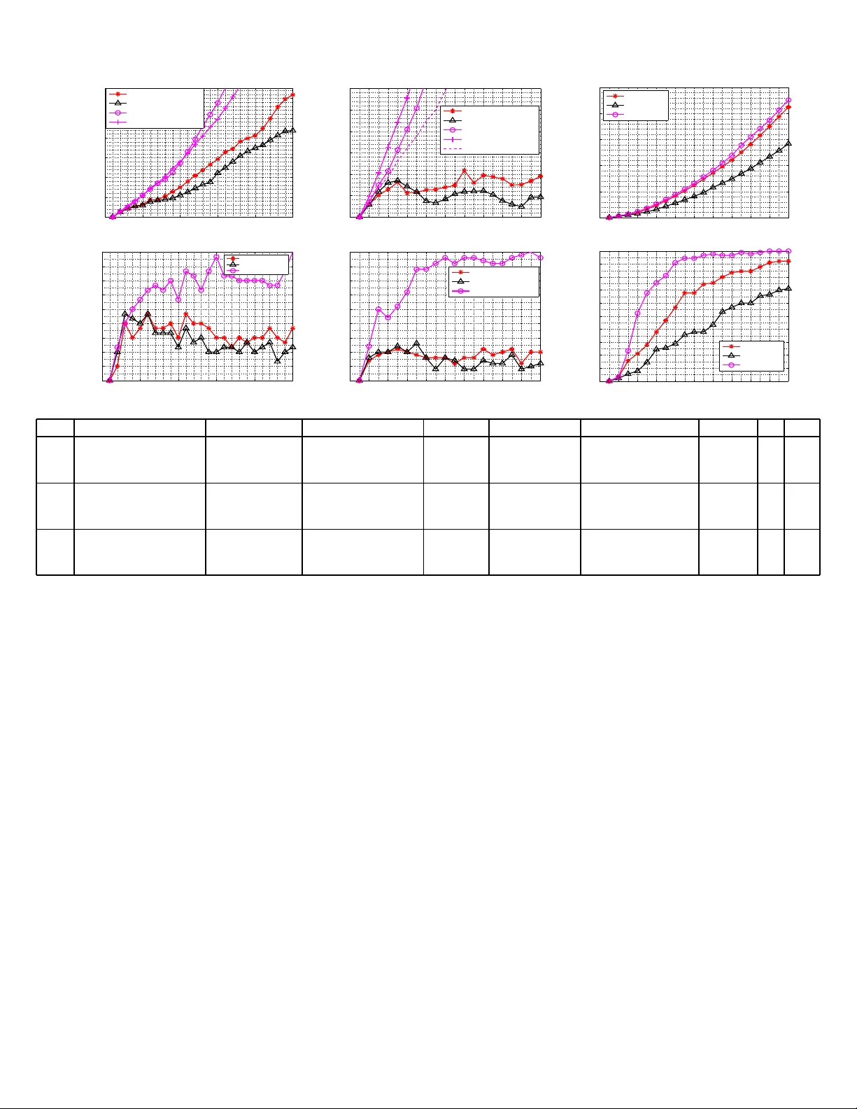
1 P articl e Filteri ng for Lar ge Dimensional State Spaces with Multimodal Ob serv ation Lik elihoods Namrata V aswani Abstract — W e study efﬁcient importance sampli ng techniques fo r particle ﬁltering ( PF) when either (a) the observation like- lihood (OL) is fre quentl y multimodal or hea vy-tailed, or (b) the state space dimension is large or both. When the OL is multimodal, but the state transition pdf (STP) is narro w enough, the optimal i mportance density is usu ally un imodal. Und er th is assumption, many techniques have been proposed. But when the STP is b road, this assumption does not hold. W e study how existing techniq ues can be generalized to situations where the optimal importance den sity is mu ltimodal, but is unimodal conditioned on a part of the state vector . Sufﬁcient conditions to test for the unimodality of this condi- tional posterior are deriv ed . Our result is directly extend able to testing for unimodality of any posterior . The number of p articles, N, to accurately track using a PF increases with state space dimension, thus maki ng any regular PF impractical f or large d imensional tracking problems. But in most such p roblems, most of the state change occurs in only a few dimensions, whi le the change in the rest of the dimensions is small. Usi ng th is property , we propose to replace importance sampling fr om a large p art of the state space (whose conditional posterior is narro w enough) by just tracking the mode of the conditional posterior . This introduces some extra error , but i t also greatly reduces the importance sampli ng dimension. The net effect is much smaller error fo r a given N, especially when the a vailable N is small. An important class of l arge dimensional p roblems with multi modal OL is tracking spatially vary ing physical quantities su ch as temperatur e or pressure in a large area using a network of sensors which may be nonlinear and/or may have non-negligible failure probabilities. Improv ed perfo rmance of our proposed algorithms ov er existing PF s is demonstrated for this problem. I . I N T RO D U C T I O N T racking is the p roblem of causally estimating a h idden state sequence , { X t } , fr om a sequ ence o f noisy and p ossibly nonlinear o bservations, { Y t } th at satisfy the Hidd en Markov Model (HMM) assumption. A tracker recursi vely co mputes (or approx imates) the “posterior” at time t , using the posterio r at t − 1 and the curren t obser vation Y t . For no nlinear an d/or no n- Gaussian state space mod els, the posterior cannot be comp uted exactly . But, it can be efﬁciently approximated using a se- quential Mo nte Carlo method called particle ﬁltering (PF) [ 3], [4], [5]. A PF ou tputs at each time t , a cloud of N weighted particles whose empirical m easure closely approxim ates the true posterior for large N . A generic PF is summarized in Algorith m 1. T here are two main issues in PF design: (a) c hoice of impor tance sampling d ensity that redu ces the variance o f the particle weights an d thus impr oves “effecti ve particle size” [6] and (b) choice of resampling techniq ues N. V aswani is with the Dept. of Electric al and Computer Engineering, Iow a State Uni versit y , Ames, IA 50011 (email: namrata@iasta te.edu). A pa rt of this pape r is c ontained in [1 ]. Some initial ide as appeare d in [2]. that improve effecti ve par ticle size wh ile not sign iﬁcantly increasing “pa rticle impoverishmen t” [4]. Some solutions f or (b) are [5, Ch. 13 ],[7], [8]. Our focus is on designing efﬁcient importan ce de nsities and analyzing the assumptions under which they work, when either or both of the following occu r: 1) The observation likelihoo d (OL) is freque ntly multi- modal or heavy-tailed (or most gener ally , no t strongly log-con cav e) as a function of the state and th e state transition pr ior (STP) is bro ad. 2) State space dimension is large (typically more than 10 o r 12). It is well known [3], [9] th at the n umber of particles for a given tracking accuracy increases with state space dimension. This m akes any regular PF imp ractical for large dimensiona l state spaces (LDSS) . Deﬁnition 1 ( Multimodal (o r heavy- tailed) OL): ref ers to the OL, p ( Y t | X t ) , having multiple local maxima (or a heavy tail) as a functio n o f the state, X t , for a gi ven observ ation, Y t . An example is the observation model for the nonstationary growth mod el of [ 3]: Y t = X 2 t + w t . Here, the OL is b imodal with m odes a t X t = ± √ Y t whenever Y t is sig niﬁcantly positive. Another example is the clutter mode l of [1 0]. Other examp les ar e as f ollows. Con sider track ing spatially varying temper ature chang e using a network of sensors ( see Example 1). Wh enever o ne or mo re sensors fail (e.g. due to a large u nmode led disturban ce or som e other d amage), the OL is ofte n heavy-tailed or mu ltimodal (see Fig. 1). The mo dels of Exa mple 1 are also similar to the com monly used clutter model in rad ar ba sed target trac king application s or in co ntour tracking applications, e. g. Condensation [10], an d to o utlier noise models used in other visual tracking problem s [11] or in airc raft navigation prob lems [9]. A nother r eason for OL multimoda lity is having a sensor that measur es a nonlin ear (many-to-o ne) functio n of the actual temperature. For e.g ., the growth model of [3 ]. Ano ther m any-to-on e example is when the observation is a pro duct of functions o f two subsets of states plus noise, for e.g. bearings-on ly trackin g [3] o r illumination a nd m otion trackin g [12], [13]. Note that even though our w ork was motiv ated by tracking problem s with fre quently mu ltimodal OL, it is equally well applicab le to any pr ob lem where the po sterior is often mu lti- modal (e. g. due to nonline arities in the system model) , b ut is unimoda l conditioned o n a part of the state sp ace . Large dimen sional state spaces ( LDSS) occur in tracking time-varying rand om ﬁelds, such as temper ature o r pressure, at a large numb er of no des using a network o f sen sors [14], [15] (ap plications in environment monitoring and weath er forecasting ); in tr acking AR parameters fo r noisy spee ch [16]; and in visual trac king pro blems such as trackin g deform ing contour s [17], [ 18], [1 9], [1 1], tr acking spatially varying 2 −15 −10 −5 0 5 10 15 0 10 20 30 40 50 State, X t → −log PDF(X t ) Narrow prior: Unimodal posterior −log[OL] −log[STP] −log[p*(X t )] (a) Bimodal OL, Narrow STP: Unimodal p ∗ −15 −10 −5 0 5 10 15 0 10 20 30 40 50 State, X t → −log PDF(X t ) Broad prior: Multimodal posterior −log[OL] −log[STP] −log[p*(X t )] (b) Bimodal OL, Broad ST P: Bimodal p ∗ −15 −10 −5 0 5 10 15 0 10 20 30 40 50 X t −log PDF(X t ) Broad STP: Multimodal p* −log[OL] −log[STP] −log[p * (X t )] (c) Heavy -tailed OL, Broad STP: Bimodal p ∗ Fig. 1. Demonstrating the effec t of multimodal or heavy-tailed OL and broad STP for a M = 1 dimensional version of Example 1 with temperature independent failure. X t is temperature. The STP is N ( X t − 1 , σ 2 sy s ) , i.e. E xample 1 with a = 0 . Fig. 1(a): One out of J = 2 sensors fails (bimodal OL) but narrow enough STP ( σ 2 sy s = 1 ). S o p ∗ is unimodal. Fig. 1(b): One out of J = 2 sensors fails (bimodal OL) and broad S TP ( σ 2 sy s = 5 ). So p ∗ is bimodal. Fi g. 1(c): Estimating temperature but wit h J = 1 sensor and broad STP ( σ 2 sy s = 5 ). When the sensor fails, the OL is heavy-tailed and peaks at the wrong mode. T hus p ∗ is bimodal with the wrong mode being the strong one. Note that the correct mode is so weak it may get missed in numerical computations. illumination c hange [1 2], [13] or tr acking sets o f “land mark” points [20]. In all of the above pro blems, at a ny time, “most state change” occurs in a small numb er of dimensions, while the chan ge in the rest of the sta te space is small. W e call this the “LDSS pr operty . The LDSS prop erty is r elated to , but different from, the assumption used by dimen sion reductio n technique s such a s Princip al Com ponen ts Analysis (PCA). If X t is a station ary large dimensional time series, or if X t projected alon g a large part of the state space is asymp totically stationary , PCA can be used f or dimension redu ction. Un der a similar assumption , ano ther PF h as been recently pro posed [21]. But if X t follows a rando m walk mo del (the inc rements, X t − X t − 1 , are station ary) in a ll dimensions, one cann ot simply eliminate the lo w variance direction s of X t − X t − 1 , or use [21]. This is beca use the variance of X t ev en alon g these directions will b e sig niﬁcant as t increases. A generic PF is summariz ed in Algorith m 1. The most common ly used imp ortance sampling density is the STP [3]. This a ssumes nothin g and is easiest to imp lement. But since this d oes not use knowledge of th e observation, the weigh ts’ variance c an be large (p articularly when th e STP is broad compare d to the OL), resulting in lower effective p article sizes [4]. T he “optimal” importan ce density [6 ], i.e. one th at min - imizes the variance of weig hts condition ed on past par ticles and o bservations un til t , is the posterior condition ed on the previous state, d enoted p ∗ . When p ∗ is unimodal ( at least approx imately), PF-Do ucet [ 6] ap proxim ates it b y a Gau ssian about its mode (L aplace’ s ap proxima tion) and importan ce samples from the Gaussian. Laplace’ s appro ximation has also been u sed for ap proxim ating po steriors in dif ferent con texts earlier [2 2], [23], [ 24]. Other work in PF literature that a lso implicitly assumes that p ∗ is u nimodal includes [4], [25], [26]. When the OL is m ultimodal, p ∗ will b e u nimoda l o nly if the STP is unimodal and narrow enoug h (see Fig. 1). In many situations, espec ially for LDSS problem s, th is does n ot hold . W e develop the PF with Efﬁ cient IS (PF-EIS) algorithm to address such situation s. PF-EIS assumes unim odality of p ∗ condition ed on a fe w states which we call “multimodal s tates” . Sufﬁcient co nditions to test for the unimodality of this condition al posterior are derived in Th eorem 1. T o the b est of o ur knowledge, such a result h as not b een proved ear lier . I t is eq ually ap plicable to test for unimod ality o f any p osterior . When in addition to multimodality , the state space space dimension is also large (typ ically mo re than 10 or 12 ), the number of particles req uired for rea sonable accuracy is very large [3], [9] and this makes a regular PF impractical. One solution tha t partially addr esses this issue is [5, Ch 13 ] or [7] which prop ose to resamp le more than once within a time interval. But more resamp ling r esults in more particle impov- erishment [4]. When the state space model is c onditiona lly linear-Gaussian, or when many states can be vector quantized into a few discrete centers (need to know the centers a- priori), Rao Blackwellization (RB-PF) [ 27], [9] can be used. In gene ral, n either assum ption may hold. But when the L DSS proper ty holds, it is p ossible to split the state space in su ch a way t hat the conditional posterior of a part of it is quite n arrow , besides being unimodal. If it is na rrow enou gh, impo rtance sampling (IS) from this part of the state space can be replaced by just trackin g the mode of the cond itional posterior ( mode tracking (MT) ). The resu lting algorith m is called PF-EIS-MT . MT introdu ces some extra er ror . But it greatly reduces the IS dimension. T he n et effect, is that a much smaller nu mber of particles are requir ed to achieve a given error, thus makin g PF practical for L DSS pr oblems. In summary , our contributions ar e (a) two efﬁcient algo- rithms for multimod al and large dimen sional p roblems, (PF- EIS and PF-EI S-MT); and (b) a set o f su fﬁcient conditio ns to test for u nimodality o f the condition al p osterior (Th eorem 1) and heuristics based on it to split the state space in the most efﬁcient way . PF-EIS and Theor em 1 are derived in Sec. II. A ge neric L DSS mo del is introd uced in Sec. III. Practical ways o f choosing the “multimod al states” are d iscussed in Sec. IV. PF-EIS-MT and PF-MT are introduc ed in Sec. V. Relation to existing work is descr ibed in Sec. VI. In Sec. VII, we given extensive simulation results comp aring ou r me thods with existing work for the temper ature ﬁeld trackin g prob lem. Conclusions and op en issues are presen ted in Sec. VII I. I I . P F - E I S : P F - E FFI C I E N T I M P O RTA N C E S A M P L I N G W e den ote the prob ability density fun ction ( pdf) of a random vecto r X , f X ( X ) , using the notation p ( X ) a nd we denote th e con ditional p df, f X | Y ( X | Y ) , by p ( X | Y ) . Con sider tracking a hidden sequ ence of states X t from a sequen ce o f observations Y t which satisfy th e HMM pro perty: 3 Algorithm 1 Generic PF . Going fr om π N t − 1 to π N t ( X t ) , P N i =1 w ( i ) t δ ( X t − X i t ) (note δ ( X − a ) denotes a Dirac delta function at a ) A PF starts with sam pling N times f rom π 0 at t = 0 to ap proxim ate it by π N t ( X 0 ) . For ea ch t > 0 , it appr oximates the Bayes recursion f or g oing fro m π N t − 1 to π N t using seq uential im portance samplin g. Th is consists of th e following 3 steps: 1) Importance Sample (IS ): For i = 1 , 2 ...N , Sample X i t ∼ q ( X i t ) . T he IS den sity , q , can depend on X i 1: t − 1 , Y 1: t . 2) W eig ht: For i = 1 , 2 ...N , co mpute the weigh ts: w i t = ˜ w i t P N j =1 ˜ w ( j ) t , where ˜ w i t = w i t − 1 p ( Y t | X i t ) p ( X i t | X i t − 1 ) q ( X i t ) . 3) Resample: Replicate pa rticles in pro portion to their weights & r eset w i t for all i [4]. Set t ← t + 1 & go to step 1. Assumption 1 (HMM): For each t , 1) The dependen ce X t − 1 → X t is Markovian, with state transition pdf (STP), p ( X t | X t − 1 ) . 2) Conditioned on X t , Y t is indep endent o f p ast and f uture states and observations. The observation likelihood (OL) is p ( Y t | X t ) . A g eneric par ticle ﬁlter (PF) is summarized in A lgorithm 1. A. PF-E IS Algorithm Consider designing a PF fo r a g i ven state space model. The optimal imp ortance samp ling density [6] is p ( X t | X i t − 1 , Y t ) , p ∗ ( X t ) . In most cases, th is c annot b e compu ted analy ti- cally [6]. If p ∗ is un imodal (at least appr o ximately) , [6] suggests appr oximating it by a Gaussian abou t its mod e and sampling from it (L aplace’ s approxima tion [ 24]). But, when the OL is multim odal, or h eavy-tailed, or other wise not strongly log-concave, p ∗ will be unimodal o nly if the STP is unimo dal and n arrow en ough an d the predicted state particle is near en ough to an OL mod e (see Fig. 1). In many situation s, this may not ho ld in all dime nsions. But in most such situation s, the STP is broad and/or multimo dal in only a few directions of th e state space which we call the “multimodal” d ir ectio ns . I t can be shown that if the STP is unimod al and narrow en ough in the rest o f the d irections, p ∗ will be unimo dal cond itioned on the “multimo dal states” (Theor em 1). When this holds, we prop ose to split the state vector as X t = [ X t,s ; X t,r ] in such a way th at X t,s contains the m inimum numb er o f dimensio ns for wh ich p ∗ is unim odal condition ed o n it, i.e. p ∗∗ ,i ( X t,r ) , p ∗ ( X t | X i t,s ) = p ( X t,r | X i t − 1 , X i t,s , Y t ) (1) is unim odal. W e samp le X t,s from its STP (to samp le the p os- sibly multiple m odes of p ∗ ), an d u se Laplace’ s ap proxim ation to appro ximate p ∗∗ ,i and sample X t,r from it, i.e. samp le X i t,r from N ( m i t , Σ i I S ) wh ere m i t = m i t ( X i t − 1 , X i t,s , Y t ) , min X t,r L i ( X t,r ) , where, Σ i I S , [( ∇ 2 L i )( m i t )] − 1 L i ( X t,r ) , − log[ p ∗∗ ,i ( X t,r )] + const (2) ∇ 2 L i denotes th e Hessian of L i . Th e weig hting step also changes to satisfy the princip le of importan ce sampling. The complete algor ithm is given in Algorith m 2. W e ca ll it PF with Efﬁcient I mportan ce Sampling (PF-EIS). As we shall see later , it is very expensi ve to exactly verify the unim odality condition s of Th eorem 1. But ev en if X t,s is cho sen so that p ∗∗ ,i is unimod al for most par ticles an d at most times (i.e. is unimod al with high probab ility), the prop osed alg orithm w orks well. This c an be seen fro m the simulation re sults of Sec. VII. B. Conditio nal P osterior Unimo dality W e derive sufﬁcient condition s for u nimodality of the condi- tional posterio r , p ∗∗ ,i . Let dim( X t,s ) , K , dim( X t,r ) , M r , dim( X t ) , M = K + M r . Because of the HMM structur e, p ∗∗ ,i ( X t,r ) = ζ p ( Y t | X i t,s , X t,r ) p ( X t,r | X i t − 1 , X i t,s ) (3) where ζ is a propo rtionality co nstant. Deﬁnition 2 : W e ﬁrst deﬁne a f e w terms an d sym bols. 1) The notatio n A > 0 ( A ≥ 0 ) wh ere A is a squ are m atrix means th at A is p ositive deﬁ nite (po sitive semi-deﬁn ite) . Also, A > B ( A ≥ B ) m eans A − B > 0 ( A − B ≥ 0 ) . 2) The ter m “minimizer” refers to the un constrained loca l minimizer of a function, i.e. a p oint x 0 s.t. f ( x 0 ) ≤ f ( x ) ∀ x in its neig hborh ood. Similarly for “maximizer” . 3) A twice differentiable function , f ( x ) , is str ongly conve x in a region R , if there exists an m > 0 s.t. at all points, x ∈ R , the Hessian ∇ 2 f ( x ) ≥ mI . If f is stron gly conv ex in R , it h as at most on e minimizer in R and it lies in the interio r of R . If f is stro ngly-co n vex on R M , then it has exactly on e (ﬁnite) minimize r . 4) A fun ction is str ongly log-conca ve if its n egati ve log is strongly co n vex. An example is a Gaussian pdf. 5) Since a p df is an integrable f unction, it will always h av e at least one (ﬁnite) maximizer . Thus a pdf having at most one m aximizer is equivalent to it being u nimodal . 6) The sym bol E [ . ] den otes expected value. 7) W e d enote the − log of O L u sing th e symbo l E Y t , i.e. E Y t ( X t ) , − log p ( Y t | X t ) + const (4) 8) W e d enote the − log of th e STP o f X t,r as D i ( X t,r ) , − log p ( X t,r | X i t − 1 , X i t,s ) + const (5) 9) When th e STP of X t,r is stro ngly log-co ncave (assum ed in Th eorem 1) , we deno te its unique mode by f i r , f r ( X i t − 1 , X i t,s ) = arg max X t,r p ( X t,r | X i t − 1 , X i t,s ) (6 ) 10) [ z ] p or z p denotes the p th coordin ate of a vector, z . 11) max p is of ten used in place of max p =1 , 2 ,...M r . Combining (3), (4) and (5), L i ( X t,r ) can be written as L i ( X t,r ) = E Y t ( X i t,s , X t,r ) + D i ( X t,r ) (7) Now , p ∗∗ ,i ( X t,r ) will be unimo dal if and on ly if we can sh ow that L i has at most o ne minimizer . W e derive a set of sufﬁcient 4 Algorithm 2 P F-EIS. Going from π N t − 1 to π N t ( X t ) = P N i =1 w ( i ) t δ ( X t − X i t ) , X i t = [ X i t,s , X i t,r ] 1) Importance Sample X t,s : ∀ i , sample X i t,s ∼ p ( X i t,s | X i t − 1 ) . 2) Efﬁcient Importanc e S ample X t,r : ∀ i , samp le X i t,r ∼ N ( X i t,r ; m i t , Σ i I S ) . Here m i t ( X i t − 1 , X i t,s , Y t ) = arg min X t,r L i ( X t,r ) an d Σ i I S , ( ∇ 2 L i ( m i t )) − 1 and L i is deﬁned in ( 7). 3) W eig ht: ∀ i , co mpute w i t = ˜ w i t P N j =1 ˜ w j t where ˜ w i t = w i t − 1 p ( Y t | X i t ) p ( X i t,r | X i t − 1 ,X i t,s ) N ( X i t,r ; m i t , Σ i I S ) where X i t = [ X i t,s , X i t,r ] . 4) Resample [4]. Set t ← t + 1 & go to step 1 . condition s o n E Y t , D i and f i r to en sure th is. T he main idea is as f ollows. W e assume stro ng log -concavity (e.g. Gaussianity) of the STP of X t,r . Thus D i ( X t,r ) will be stron gly conve x with a u nique minimizer at f i r . But E Y t ( X t ) (and so E Y t as a function of X t,r ) can h av e multiple m inimizers since OL can be m ultimodal. Assume tha t E Y t ( X i t,s , X t,r ) is locally co n vex in the neig hborh ood of f i r (this will ho ld if f i r is clo se eno ugh to any o f its minim izers). Denote this region by R LC . Thu s, inside R LC , L i will be strongly con vex and hen ce it will have at mo st one minim izer . W e sh ow th at if max p | [ ∇ D ] p | is large e nough outside R LC (the spre ad of the STP o f X t,r is small en ough) , L i will have no stationar y poin ts (and h ence no m inimizers) ou tside R LC or o n its bo undar y . This id ea leads to Theorem 1 b elow . Its ﬁrst condition ensures stron g conv exity of D i ev erywher e. The secon d one ensures that R LC exists. Th e thir d o ne ensures that ∃ an ǫ 0 > 0 , s.t. at all poin ts in R c LC (complem ent of R LC ), max p | [ ∇ L i ] p | > ǫ 0 (i.e. L i has no station ary poin ts in R c LC ). Theor em 1: p ∗∗ ,i ( X t,r ) is u nimodal with th e u nique mode lying inside R LC if Assumption 1 an d the following hold: 1) The STP o f X t,r , p ( X t,r | X i t − 1 , X i t,s ) , is stro ngly log- concave. Its uniq ue mode is denoted b y f i r . 2) The − log of OL giv en X i t,s , E Y t ( X i t,s , X t,r ) is twice continuo usly differentiable almost e verywh ere and is locally conve x in th e neighb orhoo d of f i r . Let R LC ⊆ R M r denote the largest convex region in th e n eighbor- hood of f i r where ∇ 2 X t,r E Y t ( X i t,s , X t,r ) ≥ 0 ( E Y t as a function of X t,r is locally conv ex). 3) There exists an ǫ 0 > 0 such that inf X t,r ∈∩ M r p =1 ( A p ∪Z p ) max p =1 ,...M r [ γ p ( X t,r )] > 1 (8) where γ p ( X t,r ) ,      | [ ∇ D i ] p | ǫ 0 + | [ ∇ E Y t ] p | , if X t,r ∈ A p | [ ∇ D i ] p | ǫ 0 −| [ ∇ E Y t ] p | , if X t,r ∈ Z p (9) A p , { X t,r ∈ R c LC : [ ∇ D i ] p . [ ∇ E Y t ] p < 0 } Z p , { X t,r ∈ R c LC : [ ∇ E Y t ] p . [ ∇ D i ] p ≥ 0 & | [ ∇ E Y t ] p | < ǫ 0 } ( 10) ∇ E Y t , ∇ X t,r E Y t ( X i t,s , X t,r ) ∇ D i , ∇ X t,r D i ( X t,r ) (11) Pr oof: In the proo f, ∇ is used to denote ∇ X t,r . Also, we remove th e su perscripts f rom L i and D i . p ∗∗ ,i ( X t,r ) will be unimod al iff L d eﬁned in (7) has at most o ne m inimizer . W e obtain sufﬁcient cond itions for this. Cond ition 1) ensur es that D is stro ngly co n vex e verywher e with a uniqu e minimizer at f i r . Condition 2 ) e nsures th at R LC exists. By deﬁnition of R LC , E Y t is conv ex in side it. Thus the ﬁrst two cond itions ensure tha t L is strongly conve x in side R LC . So it has at most one m inimizer inside R LC . W e now show that if co ndition 3) also ho lds, L will have no stationar y points (and h ence no m inimizers) in R c LC or o n its bo undar y . A sufﬁcient condition for this is: ∃ ǫ 0 > 0 s.t. max p | [ ∇ L ] p | > ǫ 0 , ∀ X t,r ∈ R c LC (12) W e show th at condition 3 ) is sufﬁcient to ensu re (1 2). No te that ∇ L = ∇ E Y t + ∇ D . In the regions wh ere for a t least o ne p , [ ∇ E Y t ] p . [ ∇ D ] p ≥ 0 (have same sign) and | [ ∇ E Y t ] p | > ǫ 0 , condition (1 2) will always h old. Thus we only n eed to worry about regions wher e, for all p , either [ ∇ E Y t ] p . [ ∇ D ] p < 0 or [ ∇ E Y t ] p . [ ∇ D ] p ≥ 0 but | [ ∇ E Y t ] p | < ǫ 0 . This is the region ∩ M r p =1 ( A p ∪ Z p ) , G , A p , Z p deﬁned in (1 0) (13) Now , D o nly h as o ne stationary point which is f i r and it lies inside R LC (by deﬁnition of R LC ), and n one in R c LC . Thu s ∇ D 6 = 0 in R c LC and, in p articular, inside G ⊂ R c LC . Th us if we can ﬁnd a c ondition which ensures that, f or all poin ts in G , for at least on e p , [ ∇ L ] p “follows th e sign of [ ∇ D ] p ” (i.e. [ ∇ L ] p > ǫ 0 where [ ∇ D ] p > 0 and [ ∇ L ] p < − ǫ 0 where [ ∇ D ] p < 0 ), we will be do ne. W e ﬁrst ﬁnd the required co ndition for a g i ven p and a p oint X t,r ∈ G . For any p , if X t,r ∈ G , then it either b elongs to A p or b elongs to Z p . If X t,r ∈ A p , | [ ∇ L ] p | > ǫ 0 if | [ ∇ D ] p | ǫ 0 + | [ ∇ E Y t ] p | > 1 (14) This is o btained by combining the co nditions for the case [ ∇ D ] p > 0 and the case [ ∇ D ] p < 0 . Proceed ing in a similar fashion, if X t,r ∈ Z p , | [ ∇ L ] p | > ǫ 0 if | [ ∇ D ] p | ǫ 0 − | [ ∇ E Y t ] p | > 1 (15) Inequa lities (14) and (1 5) c an b e combined and re written as γ p ( X t,r ) − 1 > 0 where γ p is d eﬁned in (9). For (12) to hold, we n eed | [ ∇ L ] p | > ǫ 0 for at least on e p , for all X t,r ∈ G . This will happen if inf X t,r ∈G max p γ p ( X t,r ) > 1 . But this is con dition 3. Thu s co ndition 3) im plies that L has no minimizers in R c LC . Th us if co nditions 1), 2) and 3) of the theorem hold , L h as at most o ne minimizer w hich lies inside R LC . T hus p ∗∗ ,i ( X t,r ) has a uniqu e mod e wh ich lies inside R LC , i.e. it is unimod al.  The most comm on example of a stron gly log-co ncave p df is a Gaussian. When the STP o f X t,r is Gaussian with mean (= 5 mode) f i r , the ab ove result can be furth er simpliﬁed to get an upper bou nd on the eigenv alues of its covariance m atrix. First consider the case when the cov aria nce is diagon al, d enoted ∆ r . In this case, D i ( X t,r ) = P p ([ X t,r − f i r ] p ) 2 2∆ r,p and so [ ∇ D i ] p = [ X t,r − f i r ] p ∆ r,p . By substituting this in con dition 3), it is easy to see th at we g et the following simpliﬁed cond ition: inf X t,r ∈∩ M r p =1 ( A p ∪Z p ) max p [ γ num p ( X t,r ) − ∆ r,p ] > 0 (16) γ num p ( X t,r ) ,      | [ X t,r − f i r ] p | ǫ 0 + | [ ∇ E Y t ] p | , if X t,r ∈ A p | [ X t,r − f i r ] p ǫ 0 −| [ ∇ E Y t ] p | , if X t,r ∈ Z p (17) A p , { X t,r ∈ R c LC : [ X t,r − f i r ] p . [ ∇ E Y t ] p < 0 } Z p , { X t,r ∈ R c LC : [ ∇ E Y t ] p . [ X t,r − f i r ] p ≥ 0 & | [ ∇ E Y t ] p | < ǫ 0 } (18) Also, since max p [ g 1 ( p ) − g 2 ( p )] ≥ max p g 1 ( p ) − max p g 2 ( p ) for any two f unctions, g 1 , g 2 , a sufﬁcient co ndition f or ( 16) is max p ∆ r,p < inf X t,r ∈∩ M r p =1 ( A p ∪Z p ) max p [ γ num p ( X t,r )] , ∆ ∗ (19) Thus, we h av e the following coro llary . Cor ollary 1: When the STP o f X t,r is Gau ssian with mean f i r and diagonal covariance, ∆ r , p ∗∗ ,i ( X t,r ) is un imodal if (a) conditio n 2) of Theo rem 1 ho lds an d ( b) there exists an ǫ 0 > 0 s.t. (16) ho lds with γ num p deﬁned in (17) and A p , Z p deﬁned in (1 8). A sufﬁcient cond ition for (16) is (19). Now consider the case when the STP of X t,r is Gaus- sian with non-diag onal covariance, Σ r = U ∆ r U T . Deﬁn e ˜ X t,r = U T X t,r . Since ˜ X t,r is a one-to -one and linear function of X t,r , it is easy to see th at p ∗∗ ,i ( X t,r ) is unimodal iff p ∗∗ ,i ( ˜ X t,r ) , p ( ˜ X t,r | X i t − 1 , X i t,s , Y t ) is unim odal. Th e STP of ˜ X t,r is N ( U T f i r , ∆ r ) . Also, its OL is p ( Y t | X i t,s , U ˜ X t,r ) . Deﬁne ˜ E Y t ( ˜ X t,r ) , E Y t ( U ˜ X t,r ) . Cor ollary 2: When the STP o f X t,r is Gau ssian with mean f i r and non- diagonal covariance, Σ r = U ∆ r U T , p ∗∗ ,i ( X t,r ) is unimodal if the condition s of Corollary 1 hold with E Y t replaced by ˜ E Y t ; f i r replaced by U T f i r and X t,r replaced by ˜ X t,r ev erywher e. T o summar ize the above discussion, p ∗∗ ,i is unimod al if 1) The STP of X t,r is strongly log-con cav e (e.g. Gaussian), 2) The mode of the STP of X t,r is “close enough ” to a mode of [O L gi ven X i t,s ], so that condition 2) of Theorem 1 ho lds. Deno te this mod e b y X ∗ r . 3) The max imum spread of the STP of X t,r is “small enoug h” to ensure that con dition 3) o f Theore m 1 holds. In the Gau ssian STP case, this translates to the maxim um eigenv alu e of its covariance be ing smaller than ∆ ∗ , deﬁned in (1 9). ∆ ∗ itself is directly propor tional to th e distance of X ∗ r to th e n ext near est mo de of [OL given X i t,s ] and inversely p roportio nal to its strength. The last two cond itions a bove automa tically hold if [OL g iven X i t,s ] is str ongly log-concav e ( R c LC is empty and s o ∆ ∗ = ∞ ). I I I . A G E N E R I C S TA T E S PAC E M O D E L F O R L D S S For many pro blems, an d, in particu lar , for many large dimensiona l state space (LD SS) pro blems, the state space model ca n be expressed as follows with X t = [ C t , v t ] (a generalizatio n of the con stant velocity mo tion mode l): Y t = h C,w ( C t , w t ) , w t ∼ p w ( . ) C t = C t − 1 + g C t − 1 ( B v t ) , B , B ( C t − 1 ) v t = f v ( v t − 1 ) + ν t , ν t ∼ N (0 , ∆ ν ) , ∆ ν diagona l (20) The no ises ν t , w t are indep endent of each othe r and over time. If h C,w is one -to-one as a function of w t , an d its inverse is denoted by g ( C t , Y t ) , th e OL can be written as p ( Y t | C t ) = p w ( g ( C t , Y t )) (21) Then its − log , E Y t ( C t ) = − log p w ( g ( C t , Y t )) . In cer- tain problems, it is easier to directly specify p ( Y t | C t ) = β ex p[ − E Y t ( C t )] . In th e above mo del, C t denotes the LDSS quantity of interest, for e.g. it m ay deno te the M con tour point locations or it may denote tempera ture ( or any other p hysical quantity) at M sensor node s. The quantity V t , B v t often denotes the time “derivati ve” of C t and is assumed to f ollow a ﬁrst o rder Mar kov m odel. If C t belongs to a smooth manifold S , then V t belongs to the tangent space to S at C t . g C ( V ) denotes the mapp ing fro m the tan gent sp ace at C to S , while if S is a vector sp ace, then g C ( V ) ≡ V . In this work, we only study the vector space case. W e d ev elop the same ideas for the sp ace of contou rs (a smooth ma nifold) in [1 1]. Related work on deﬁnin g AR m odels f or smo oth m anifolds is [28]. Note that in the above model, the system noise d imension (and hence th e importance sampling d imension) is M = dim( ν t ) = dim( v t ) , an d not 2 M , an d this is what g overns the nu mber of particles req uired for a giv en accur acy . W e d iscuss som e LDSS examp les b elow . Example 1 (T emperature T racking): Consider tracking temperatur e at M loc ations using a n etwork of sensors. Here S is a vector space and so g C ( V ) ≡ V . Let C t,p denotes temperatur e at locatio n p , p = 1 , . . . M an d V t,p denote the ﬁrst d eriv a ti ve of temper ature at no de p . V t is assumed to be zero mean an d its dy namics can be mod eled by a linear Gauss M arkov m odel (as also in [ 14]), i.e . C t = C t − 1 + V t , V t = A V V t − 1 + n t , n t ∼ N (0 , Σ n ) ( 22) Since V t is u sually spatially correlated, Σ n may not be diagona l. Let the eigenvalue deco mposition of Σ n is Σ n = B ∆ ν B T . Deﬁne v t , B T V t , ν t , B T n t , f v ( v ) ≡ B T A V B v and g C ( V ) ≡ V . For simplicity , we use A V = aI an d so f v ( v ) ≡ B T A V B v = av . W ith f v ( v ) = av , B is also the eigenv ector matrix of the covariance of V t . Then (22) can be rewritten in the fo rm (20) as C t = C t − 1 + B v t v t = av t − 1 + ν t , ν t ∼ N (0 , ∆ ν ) (23) T em perature at each node, p , is measur ed using J ( J = 1 or 2) sensors tha t have failure probabilities α ( j ) p , j = 1 , 2 . Note tha t th ere m ay actually b e two senso rs at a nod e, or two nearby senso rs can be combin ed and treated as one “node” 6 for trackin g purpo ses. Failure of the J M sensors is assumed to be independ ent of each other and over time. If a sensor is working , the ob servation, Y ( j ) t,p , is the actual temperature, C t,p , or some function of it, h p ( C t,p ) , plus Gaussian noise with small variance, σ 2 obs,p (indepen dent of noise in other sensors and at other times). If the senso r fails, Y ( j ) t,p is either indepen dent of , or weakly depend ent on C t,p (e.g. large variance Gaussian about C t,p ). An alternative failure mod el is Y ( j ) t,p being some different f unction, h f p , of C t,p plus no ise. In all the ab ove cases, the OL c an be wr itten as p ( Y t | C t ) = M Y p =1 J Y j =1 p ( Y ( j ) t,p | C t,p ) , wher e p ( Y ( j ) t,p | C t,p ) = (1 − α ( j ) p ) N ( Y ( j ) t,p ; h p ( C t,p ) , σ 2 obs,p ) + α ( j ) p p f ( Y ( j ) t,p | C t,p ) (24) W e simulated two typ es of senso rs h p ( C t,p ) = C t,p (linear) and h p ( C t,p ) = C 2 t,p (squared ). Note that a squared sensor is an extreme example of possible sensing nonlin earities. First consider J = 1 (on e sensor per n ode), h p ( C t,p ) = C t,p , ∀ p (all line ar senso rs), an d p f ( Y ( j ) t,p | C t,p ) = p f ( Y ( j ) t,p ) (when the sensor fails, the observation is in depend ent of the true temperatur e). In this case, each O L term is a raised Gaussian (heavy-tailed) as a fun ction of C t,p and so it is n ot strong ly log-con cav e. For a given p , p ∗ ( C t,p ) will be mu ltimodal when Y (1) t,p is “far” from the pr edicted tempera ture at this node and the STP is not narr ow enou gh. Th is happ ens with high probab ility ( w .h.p.) whe nev er the sensor fails. See Fig. 1(c). A similar m odel is also used in m odeling clu tter [1 0], [20]. Now consider J = 2 , all linear sensors and p f ( Y ( j ) t,p | C t,p ) = p f ( Y ( j ) t,p ) . Whenever one or bo th sensors at a nod e p 0 fail, the observations Y (1) t,p 0 , Y (2) t,p 0 will be “far” co mpared to σ 2 obs w .h.p. In this ca se, the OL will be bim odal as a fun ction of C t,p 0 since p ( Y t,p | C t,p ) can be written as a su m of four terms: a pr oduct o f Gaussians term (which is n egligible), plus K 1 + K 2 N ( Y (1) t,p 0 ; C t,p 0 , σ 2 obs ) + K 3 N ( Y (2) t,p 0 ; C t,p 0 , σ 2 obs ) where K 1 , K 2 , K 3 are constants w .r .t. C t . This is bimod al since the modes of the two Ga ussians, Y (1) t,p 0 , Y (2) t,p 0 , are “far”. See Fig. 1 (b). I f no sensor at a node fails, bo th ob servations will be “close” w . h.p.. In this case all four terms h av e rough ly th e same mode, and thus th e su m is u nimoda l. When p f ( Y ( j ) t,p | C t,p ) is weakly dependent on C t,p (e.g. a large variance Gaussian), K 1 , K 2 , K 3 are n ot co nstants but are slowly varying functions of C t . A similar argument applies there a s well. A squared sen sor r esults in a bimo dal OL whenever Y ( j ) t,p is sig niﬁcantly p ositi ve. Sq uared sen sor is one examp le of a many-to-o ne m easurement fu nction. Other examples inc lude bearings-o nly tracking [3] and illumination trac king [12], [13]. Example 2 (I llumination/Mo tion T racking): T he illumin a- tion an d m otion track ing m odel of [12], [13] can be rewritten in the form (20). In this case, the OL is of ten multimo dal since the o bservation (image in tensity) is a m any-to-on e function of the state (illuminatio n, motion ), but co nditioned on motion, it is of ten un imodal. Th e STP of illumination is qu ite n arrow . Example 3 (Con tour T racking, Landmark S hape T racking): T wo non -Euclidean space exam ples of the LDSS m odel (2 0) are (a) the con tour track ing pro blems g i ven in [11], [29], [17] and ( b) th e landm ark shape trackin g problem of [ 20], [1 0]. I V . C H O O S I N G T H E “ M U LT I M O D A L S T A T E S ” F O R L D S S In Sec.IV - A below , we app ly Theo rem 1 to th e g eneric LDSS model, (2 0), and show a n example of verifyin g its condition s. Practical ways to select X t,s are given in Sec.IV -B. A. Unimod ality Result for LDSS m odel Consider a model of the form (20) with g C ( V ) ≡ V . Assume that v t can be partition ed into v t = [ v t,s ; v t,r ] where v t,s denotes th e temp erature chang e coefﬁcients along the “multimod al” d irections of the state space and v t,r denotes the rest. Th us, X t,s = v t,s and X t,r = [ v t,r , C t ] . Similarly partition B = [ B s , B r ] , ∆ ν = di ag (∆ ν,s , ∆ ν,r ) a nd ν t = [ ν t,s ; ν t,r ] . W e discuss how to choo se v t,s and v t,r in Sec. IV -B. Th e “m ultimodal” dime nsion, K = dim( v t,s ) and M r = M − K . Denote ˜ C i t , C i t − 1 + B s v i t,s , f i r , f v, r ( v i t − 1 ) Then we have p ∗∗ ,i ( v t,r , C t ) = p ( v t,r , C t | v i t − 1 , C i t − 1 , v i t,s , Y t ) = ζ N ( v t,r ; f i r , ∆ ν,r ) δ ( C t − [ ˜ C i t + B r v t,r ]) p ( Y t | C t ) = ζ N ( v t,r ; f i r , ∆ ν,r ) p ( Y t | ˜ C i t + B r v t,r ) δ ( C t − [ ˜ C i t + B r v t,r ]) , p ∗∗ ,i ( v t,r ) δ ( C t − [ ˜ C i t + B r v t,r ]) (25) where δ denotes th e Dirac delta function and ζ is a p ro- portion ality co nstant. Since C t is a deterministic function of C i t − 1 , v i t,s , v t,r , its pdf is a Dirac d elta f unction (which is tri v ially unimoda l at ˜ C i t + B r v t,r ). Thus for th e purpose of importan ce sam pling, X t,r = v t,r only , and we need condition s to ensure that p ∗∗ ,i ( v t,r ) is unimod al. In th is case, L i ( v t,r ) , − log p ∗∗ ,i ( v t,r ) + con st b ecomes L i ( v t,r ) , E Y t ( ˜ C i t + B r v t,r ) + M − K X p =1 ([ v t,r − f i r ] p ) 2 2∆ ν,r,p (26) Applying Coro llary 1 we get, Cor ollary 3: Conside r model (20) with g C ( V ) ≡ V . Cor ol- lary 1 ap plies with th e following substitutions: X t,s ≡ v t,s , X t,r ≡ v t,r , M r ≡ M − K , ∆ r,p ≡ ∆ ν,r,p , f i r ≡ f v, r ( v i t − 1 ) , ∇ E Y t ≡ B T r ∇ C E ( ˜ C i t + B r v t,r ) , R LC ⊆ R M − K is the largest conv ex region in the neighb orhoo d of f i r where E Y t ( ˜ C i t + B r v t,r ) is c on vex as a function of v t,r . W e de monstrate h ow to verify the conditio ns of Cor ollary 3 using a temp erature tracking example. W e use numerical (ﬁnite difference) computations of gradients. Here ǫ 0 needs to be c hosen carefu lly , de pending on the resolution of th e discretization gr id of v t,r . I t shou ld be just large enoug h 1 so that on e do es no t miss any stationa ry point of E Y t . 1 If ǫ 0 is too small, [ ∇ E Y t ] p may transition from a value sm aller than − ǫ 0 to a v alue la rger than + ǫ 0 (or vice ve rsa) o ver on e gri d po int, a nd t his r egion will not be included in Z p (e ven if [ ∇ D ] p has the same sign as [ ∇ E Y t ] p ), thus getting a wrong (too large) value of ∆ ∗ . If ǫ 0 is larger than required, the region Z p may be bigger than needed, thus givi ng a sm alle r value ∆ ∗ than what can actuall y be allo w ed. 7 R LC & the point v t−1,r i v t,r,1 v t,r,2 −10 −5 0 5 10 −15 −10 −5 0 5 10 15 (a) Regi on R LC & point f i r A 1 ∩ A 2 , ∆ *=1.79 v t,r,1 v t,r,2 −10 −5 0 5 10 −15 −10 −5 0 5 10 15 (b) A 1 ∩ A 2 Z 1 ∩ A 2 , ∆ *=1642.6 v t,r,1 v t,r,2 −10 −5 0 5 10 −15 −10 −5 0 5 10 15 (c) Z 1 ∩ A 2 Z 2 ∩ A 1 , ∆ *=403.7 v t,r,1 v t,r,2 −10 −5 0 5 10 −15 −10 −5 0 5 10 15 (d) Z 2 ∩ A 1 Z 1 ∩ Z 2 , ∆ *=4771.4 v t,r,1 v t,r,2 −10 −5 0 5 10 −15 −10 −5 0 5 10 15 (e) Z 1 ∩ Z 2 (f) E Y t ( v t,r ) v t,r,1 v t,r,2 [ ∇ E Y t ] p =0, p=1,2 −10 −8 −6 −4 −2 0 2 4 6 8 10 −15 −10 −5 0 5 10 15 [ ∇ E] 1 =0 [ ∇ E] 2 =0 (g) ( ∇ E Y t ) p = 0 , p = 1 , 2 v t,r,1 v t,r,2 [ ∇ L] p =0, p=1,2 for ∆ r,1 = ∆ r,2 =0.9 ∆ * −10 −8 −6 −4 −2 0 2 4 6 8 10 −15 −10 −5 0 5 10 15 [ ∇ L] 1 =0 [ ∇ L] 2 =0 (h) ( ∇ L ) p = 0 , ∆ r = 0 . 9∆ ∗ v t,r,1 v t,r,2 [ ∇ L] p =0, p=1,2 for ∆ r,1 = ∆ r,2 =1.1 ∆ * −10 −8 −6 −4 −2 0 2 4 6 8 10 −15 −10 −5 0 5 10 15 [ ∇ L] 1 =0 [ ∇ L] 2 =0 (i) ( ∇ L ) p = 0 , ∆ r = 1 . 1∆ ∗ Fig. 2. Computing ∆ ∗ for E xample 4. W e used α (1) = [0 . 1 , 0 . 1 , 0 . 1] , α (2) = [0 . 4 , 0 . 4 , 0 . 4] , p f ( Y ( j ) t,p ) = U nif ( − 10 , 10) , j = 1 , 2 , ∀ p , σ 2 obs = [1 , 1 , 1] , ∆ ν, 1 = 5 . 4 , B = [ − 0 . 27 , 0 . 96 , − 0 . 02] ′ ; [0 . 33 , 0 . 11 , 0 . 94] ′ ; [0 . 90 , 0 . 24 − 0 . 35] ′ (we use MA TLAB notation). Also, C i t − 1 = [0 , 0 , 0] ′ , v i t − 1 ,r = [0 0] ′ , v i t − 1 ,s = 0 , Y (1 , 2) t, 1 = [5 . 36 , 0 . 59] , Y (1 , 2) t, 2 = [ − 2 . 25 , − 1 . 60] Y (1 , 2) t, 3 = [ − 0 . 68 , 0 . 35] and v i t,s = − 3 . 2 (si mulated from N (0 , ∆ ν, 1 ) ). F ig. 2(a): r egion R LC , and the point f i r = v i t − 1 ,r which lies inside it. F ig. 2(b), 2(c), 2(d) , 2(e): the regions, A 1 ∩ A 2 , Z 1 ∩ A 2 , Z 2 ∩ A 1 and Z 1 ∩ Z 2 , along with the computed minimum v alue of max p γ p ( v t,r ) in the 4 regions (1.79, 1642.6, 403.7, 4771.4). The ﬁ nal valu e of ∆ ∗ is the minimum of these four values, i.e. ∆ ∗ = 1 . 79 . Fig 2(f): mesh plot of E Y t as a function of v t,r . Note the 2 dominant modes. Fig 2(g): contours of [ ∇ E Y t ] 1 = 0 and [ ∇ E Y t ] 2 = 0 (obtained using the contour command t o ﬁnd the zero lev el set of [ ∇ E Y t ] j , j = 1 , 2 ). The contours hav e many points of intersection (points where ∇ E Y t = 0 ), i.e. many stationary points. Fig 2(h): contours of [ ∇ L ] 1 = 0 and [ ∇ L ] 2 = 0 for L computed w ith ∆ ν, 2 = ∆ ν, 3 = 0 . 9∆ ∗ . The contours hav e only one point of i ntersection which is a minimum. Fig 2(i) : contours of of [ ∇ L ] j = 0 , j = 1 , 2 for ∆ ν, 2 = ∆ ν, 3 = 1 . 1∆ ∗ . There are 3 intersection points (2 are minima). Example 4: Consider Ex ample 1. Assume that M = 3 and OL follows (24) with h p ( C t,p ) = C t,p (linear sensors) and p f ( Y ( j ) t,p | C t,p ) = p f ( Y ( j ) t,p ) . Also, let a = 1 . In Fig. 2, we demonstra te how to verify th e cond itions of Coro llary 3. Let K = 1 , i.e M r = 2 . Assume that X t,s = v t,s = v t, 1 and v t,r = v t, 2:3 . Assum e a given value of C i t − 1 , f i r and of Y t (given in the ﬁgu re captio n). Note that Y (1) t, 1 = 5 . 36 , Y (2) t, 1 = 0 . 59 are “far” compared to σ obs, 1 = 1 an d hence the OL is multimo dal. Fig. 2(f) plots E Y t ( v t,r ) . Fig. 2(g ) p lots the contour s of [ ∇ E Y t ] p = 0 , p = 1 , 2 (th e points where the red and b lue co ntours inter sect are the stationary points of E Y t ). V eriﬁcation of co ndition 2 is shown in Fig. 2(a) . Next, we show the steps for comp uting ∆ ∗ . For M r = 2 , G = ∩ 2 p =1 ( A p ∪ Z p ) is a subset of R 2 and is a union of the 4 regions: A 1 ∩ A 2 , Z 1 ∩ A 2 , A 1 ∩ Z 2 , Z 1 ∩ Z 2 , shown in Fig 2(b), 2 (c), 2( d), 2(e). The compu ted value o f the minim um of max p γ num p ( v t,r ) in ea ch region is also giv en in the titles. The ﬁnal ∆ ∗ = 1 . 7 9 is the m inimum of these 4 v alues. Contours of [ ∇ L i ] 1 = 0 and of [ ∇ L i ] 2 = 0 com puted for ∆ ν, 2 = ∆ ν, 3 = 0 . 9 ∆ ∗ and 1 . 1∆ ∗ are shown in Figs. 2(h), 2(i). Notice that when ∆ ν, 2 = ∆ ν, 3 = 0 . 9∆ ∗ , they intersect at only one point i.e. ∇ L i = 0 at only one po int (o ne station ary point). When ∆ ν, 2 = ∆ ν, 3 = 1 . 1 ∆ ∗ , th ere are 3 stationary points ( and 2 are min ima). B. Choosin g the “Multimodal” States, X t,s Corollary 3 gives a unim odality con dition that needs to be veriﬁed separately f or each particle an d each Y t at each t . An exact a lgorithm to do this would b e to begin by check ing at each t , fo r eac h i , if Theor em 1 holds with K = 0 . Keep increasing K and doing this until ﬁnd a K for which Corollary 3 holds co nditioned on X i t, 1: K . T his can be d one efﬁciently only if ∆ ∗ can be computed analytically or using some efﬁcient num erical techniq ues. Th at will be the fo cus of future research. But, as d iscussed earlier, PF-EIS works ev en if un imodality of p ∗∗ ,i ( X t,r ) h olds for most p articles at m ost times, i.e. it hold s w .h.p. W e u se the temperatu re trac king pro blem o f Example 1 to explain how to choose X t,s . For a given K , we would like to choose X t,s = v t,s that makes it most likely for p ∗∗ ,i ( v t,r ) to be u nimodal. Giv en X i t − 1 , v i t,s , v t,r is a lin ear f unction o f C t . If v t,r were also a one-to- one f unction of C t , then o ne co uld equiv alently ﬁnd condition s for unimod ality of p ∗∗ ,i ( C t ) , which is easier to analyze. For an appr oximate an alysis, we make it a one- to-one function o f C t by add ing a very small variance (com pared to th at of any ν t,p ) no ise, n t,s , along B s , i.e. giv en X i t − 1 , v i t,s , set C t = C i t − 1 + B s v i t,s + B r v t,r + B s n t,s . Now , C t is a one-to- one and linear fun ction of [ v t,r , n t,s ] . This also makes p ∗∗ ,i ( C t ) a no n-degener ate pdf. First co nsider the case where w .h.p . OL can be multimo dal as a functio n of te mperature at only one node p 0 , for e.g., h p ( C t,p ) = C t,p , ∀ p 6 = p 0 , α j p = 0 , ∀ p 6 = p 0 , and either α j p 0 > 0 or h p 0 ( C t,p 0 ) is m any-to-on e. Then, p ∗∗ ,i ( C t ) = p ∗∗ ,i ( C t,p 0 ) z }| { ζ p ( Y t,p 0 | C t,p 0 ) p ( C t,p 0 | X i t − 1 , v i t,s ) × [ Y p 6 = p 0 p ( Y t,p | C t,p )] p ( C t | C t,p 0 , X i t − 1 , v i t,s ) (27) 8 and the last two ter ms above are G aussian (and hence strongly log-co ncave) as a function of C t,p , p 6 = p 0 . If p ∗∗ ,i ( C t,p 0 ) is also strongly log-co ncave then p ∗∗ ,i ( C t ) (and hence p ∗∗ ,i ( v t,r ) ) will b e strongly log-co ncave, an d hen ce unimod al. Now , p ∗∗ ,i ( C t,p 0 ) will be stro ngly log- concave if ∃ ǫ 0 > 0 such that ∆ C,p 0 = V ar [ p ( C t,p 0 | X i t − 1 , v i t,s )] < inf { C t : ∇ 2 C t,p 0 E Y t ( C t ) < 0 } 1 |∇ 2 C t,p 0 E Y t ( C t ) | + ǫ 0 . This bound can only b e com puted on th e ﬂy . A- priori, p ∗∗ ,i ( C t,p 0 ) will be most likely to b e log -concave if v t,s is c hosen to ensure that ∆ C,p 0 is smallest. Let v t,s = v t,k 0 where the set k 0 contains K elem ents o ut of [1 , . . . M ] and K is ﬁxed. Th en, ∆ C,p 0 = P k / ∈ k 0 B 2 p 0 ,k ∆ ν,k . This igno res the variance o f n t,s (valid since th e variance is assumed very small co mpared to all ∆ ν,p ’ s). Thus, ∆ C,p 0 will be sm allest if v t,s is ch osen as v t,s = v t,k s , k s , arg min k 0 X k / ∈ k 0 B 2 p 0 ,j ∆ ν,k (28) When K = 1 , this is equi valent to cho osing k s = arg max k B 2 p 0 ,k ∆ ν,k . Based on the a bove d iscussion, we have the following heu ristics. Heuristic 1 : If OL can be multim odal as a f unction of temperatur e at only a single node, p 0 , an d is unimodal as a function of temper ature at other n odes, select v t,s using (28). Heuristic 2 : If OL is mu ch mor e likely to b e mu ltimodal as a function o f C t,p 0 , comp ared to temper ature at any o ther node ( e.g. if a sensor at p 0 is old so that its failure prob ability is mu ch larger th an th e r est), app ly Heur istic 1 to th at p 0 . Heuristic 3 : When p 0 is a set (not a sin gle index), Heuristic 1 can be extended to select k s to minimize th e spectral radiu s (maximu m eigenv alue) of the matrix , P k / ∈ k 0 B p 0 ,k B T p 0 ,k ∆ ν,k . Heuristic 4 : If OL is eq ually likely to b e multimod al as a function of any C t,p (e.g. if all sensor s hav e eq ual failure probab ility), then p 0 = [1 , . . . M ] . Apply ing Heuristic 3, one would select the K largest variance direction s of STP as v t,s . Heuristic 5 : If the probability of OL being multimod al is itself very small, th en K = 0 c an be used. In Exam ple 1 with all linear sensors, this pr obability is roug hly 1 − Q p,j (1 − α j p ) . Heuristic 6 : For J = 2 and all linear sensors, p 0 may be chosen on-the- ﬂy as a r g max p [( Y (1) t,p − Y (2) t,p ) 2 /σ 2 obs,p ] (larger the difference, the more likely it is fo r OL to be multimo dal at th at p ). If the maxim um itself is sma ll, set K = 0 . W e sh ow an example now . Con sider Ex ample 4 w ith α (1) = α (2) = [0 . 4 , 0 . 01 , 0 . 0 1] , Σ ν = diag ([10 , 5 , 5]) , B = [0 . 95 , 0 . 21 , 0 . 21] ′ ; [ − 0 . 2 1 , 0 . 98 , − 0 . 05] ′ ; [ − 0 . 2 2 , 0 , 0 . 9 8 ] ′ (us- ing MA TL AB n otation). By Heuristic 5, the probab ility of OL being multimodal is about 0.65 which is n ot small. So we ch oose K > 0 ( K = 1 ). By Heuristic 2 , we cho ose p 0 = 1 since OL is multimo dal as a function of C t, 1 with probab ility 0.6 4, while th at for C t, 2 or C t, 3 together is 0 . 02 (much sma ller). Apply ing (28) for p 0 = 1 , we get v t,s = v t, 1 . V . P F - E I S - M T: P F - E I S W I T H M O D E T R AC K E R For any PF (includ ing efﬁcient PFs such as PF-EIS o r PF-Doucet), the effecti ve p article size [4], [6] reduces with increasing dim ension, i.e. the N requ ired for a g iv en track- ing accuracy increases with dimen sion. This makes all PFs impractically expensive for LDSS p roblems. W e discuss one possible solu tion to this pr oblem here. A. PF-E IS-MT and P F-MT Algorithm Consider the LDSS m odel ( 20). T o apply PF-EIS, we split the state X t into [ X t,s , X t,r ] , such that p ∗ is unimo dal w .h .p. condition ed on X t,s . As explained earlier , this is ensure d if th e eigenv a lues of Σ r are small enou gh to satisfy (19). Now , because of the LDSS prop erty , X t,r can f urther b e sp lit into [ X t,r,s , X t,r,r ] so th at the maximum e igen value of the covariance of th e STP of X t,r,r is small enou gh to e nsure that there is little erro r in ap proxima ting the co nditional posterior of X t,r,r by a Dirac delta function at its mode. W e call this the M ode Tracking (MT) app roximation of impor tance sampling (I S), or IS- MT . W e r efer to ˜ X t,s , [ X t,s , X t,r,s ] a s the “effective” state and to ˜ X t,r , X t,r,r as the “r esidual” state. W e explain IS- MT in detail below . In PF-EIS, we I S X i t,s from its STP , a nd we EIS X i t,r from N ( m i t , Σ i I S ) wh ere m i t , Σ i I S are deﬁned in (2). Let m i t =  m i t,s m i t,r  and Σ i I S =  Σ I S,s Σ I S,s,r Σ I S,r ,s Σ I S,r  . Th is is equ iv alent to ﬁrst samplin g X i t,r,s ∼ N ( m i t,s , Σ i I S,s ) and then samplin g X i t,r,r ∼ N ( m ∗ t,r i , Σ i I S,r ) wh ere m ∗ t,r i , m i t,r + Σ i I S,r ,s Σ i I S,s − 1 ( X i t,r,s − m i t,s ) , Σ ∗ I S,r i , Σ i I S,r − Σ i I S,r ,s Σ i I S,s − 1 Σ i I S,r ,s T (29) Now , from (29), Σ ∗ I S,r i ≤ Σ i I S,r . Also, sinc e m i t lies in a locally con vex r egion of E Y t ( X i t,s , X t,r ) , i.e. ∇ 2 E Y t ( X i t,s , m i t ) ≥ 0 (by Theor em 1), Σ i I S ≤ ∆ r . This implies that ∆ r,r − Σ i I S,r , which is a square sub-matrix of ∆ r − Σ i I S , is also no n-negative deﬁnite. Thus, Σ ∗ I S,r i ≤ Σ i I S,r ≤ ∆ r,r (30) If the m aximum eigenv alu e o f ∆ r,r is small enough, any sample fr om N ( m ∗ t,r i , Σ ∗ I S,r i ) will be clo se to m ∗ t,r i w .h.p. So we can set X i t,r,r = m ∗ t,r i with little extra error (quan tiﬁed in the next subsection) . The algorithm is then c alled PF-EI S- MT . It is summarized in Algorithm 3. A more accurate, b ut also more expensive mo diﬁcation(n eed to implem ent it on -the-ﬂy) would be do MT o n the low eigenv alue directio ns of Σ i I S . A simpler, but sometimes less accu rate, mo diﬁcation is PF-MT (summarized in Algor ithm 4). I n PF-MT , we combine X t,r,s with X t,s and imp ortance sample th e comb ined state ˜ X t,s = [ X t,s , X t,r,s ] fro m its STP (or in some cases X t,r,s is empty ), while pe rformin g mo de tracking (MT) on ˜ X t,r = X t,r,r . The IS-MT appr oximation introd uces some error in the estimate o f X t,r,r (error decreases with d ecreasing spread o f p ∗∗ ,i ( X t,r,r ) ). But it also reduces the samp ling dimension f rom dim( X t ) to dim([ X t,s ; X t,r,s ]) ( signiﬁcant red uction fo r large dimensiona l pro blems), th us improvin g the effectiv e p article size. For care fully ch osen d imension o f X t,r,r , this results in smaller total error, especially when the av ailab le numb er of particles, N , is small. This is observed experimenta lly , but proving it theoretically is an open problem. W e say that the IS-MT ap pr oxima tion is “va lid” fo r a given cho ice of X t,r,r if it re sults in smaller total e rror than if it were not used. B. IS- MT Appr oximation W e quan tify the er ror due to IS-M T . If we did not use the MT appr oximation , X i t,r,r ∼ N ( m ∗ t,r i , Σ ∗ I S,r i ) . But using MT , 9 Algorithm 3 P F-EIS-MT . Going from π N t − 1 to π N t ( X t ) = P N i =1 w ( i ) t δ ( X t − X i t ) , X i t = [ X i t,s , X i t,r ] , X i t,r = [ X i t,r,s , X i t,r,r ] 1) Importance Sample X t,s : ∀ i , sample X i t,s ∼ p ( X i t,s | X i t − 1 ) . 2) Efﬁcient Importan ce Sample X t,r,s : ∀ i , a) Co mpute m i t ( X i t − 1 , X i t,s , Y t ) = ar g min X t,r L i ( X t,r ) and Σ i I S , ( ∇ 2 L i ( m i t )) − 1 where L i is deﬁne d in (7). L et m i t =  m i t,s m i t,r  and Σ i I S =  Σ I S,s Σ I S,s,r Σ I S,r Σ I S,r ,s  . b) Sample X i t,r,s ∼ N ( m i t,s , Σ i I S,s ) . 3) Mode T rack X t,r,r : ∀ i , a) Co mpute m ∗ t,r i using ( 29). b) Set X i t,r,r = m ∗ t,r i 4) W eig ht: ∀ i , co mpute w i t = ˜ w i t P N j =1 ˜ w j t where ˜ w i t = w i t − 1 p ( Y t | X i t ) p ( X i t,r | X i t − 1 ,X i t,s ) N ( X i t,r ; m i t , Σ i I S ) where X i t,r = [ X i t,r,s , X i t,r,r ] . 5) Resample. Set t ← t + 1 and go to step 1. Algorithm 4 P F-MT . Going from π N t − 1 to π N t ( X t ) = P N i =1 w ( i ) t δ ( X t − X i t ) , X i t = [ ˜ X i t,s , ˜ X i t,r ] 1) Importance Sample ˜ X t,s : ∀ i , sample ˜ X i t,s ∼ p ( ˜ X i t,s | X i t − 1 ) . 2) Mode T rack ˜ X t,r : ∀ i , set ˜ X i t,r = m i t where m i t ( X i t − 1 , ˜ X i t,s , Y t ) = arg min ˜ X t,r L i ( ˜ X t,r ) an d L i is de ﬁned in (7). 3) W eig ht: ∀ i , co mpute w i t = ˜ w i t P N j =1 ˜ w j t where ˜ w i t = w i t − 1 p ( Y t | X i t ) p ( ˜ X i t,r | X i t − 1 , ˜ X i t,s ) where X i t = [ ˜ X i t,s , ˜ X i t,r ] . 4) Resample. Set t ← t + 1 & go to step 1. we set X i t,r,r = m ∗ t,r i . Let th e eigen value decomp osition of Σ ∗ I S,r i = U Λ ∗ I S,r i U T and let λ p , (Λ ∗ I S,r i ) p,p be its p th eigenv alu e. Let d , X i t,r,r − m ∗ t,r i . For an ǫ > 0 , we b ound the probab ility of || d || = || U T d || > ǫ using Chernoff b oundin g: P r ( || d || > ǫ ) = P r ( || U T d || > ǫ ) = P r ( e s P p ( U T d ) 2 p > e sǫ 2 ) ≤ Y p [ (1 − 2 λ p s ) − 1 / 2 e − sǫ 2 / M r,r ) ] ≤ [ (1 − 2 λ m s ) − 1 / 2 e − sǫ 2 / M r,r ) ] M r,r (31) ≤ [ (1 − 2∆ m s ) − 1 / 2 e − sǫ 2 / M r,r ) ] M r,r (32) where s > 0 , λ m , max p λ p and ∆ m , ma x p ∆ r,r ,p . The ﬁrst inequality fo llows by a pplying Markov in equality , the second follows because λ p ≤ λ m , ∀ p and (32) follows because λ m ≤ ∆ m which f ollows fr om (30). Now , (3 2) hold s for any s > 0 and thus P r ( || d || > ǫ ) ≤ [min s> 0 { (1 − 2∆ m s ) − 1 / 2 e − sǫ 2 / M r,r ) ) } ] M r,r =  ( M r,r ∆ m ǫ 2 ) − 1 e − ( ǫ 2 M r,r ∆ m − 1)  M r,r / 2 , B (∆ m , ǫ ) (33) Re writing [ B (∆ m , ǫ )] 2 / M r,r = ( M r,r ∆ m ǫ 2 ) − 1 /e ( ǫ 2 M r,r ∆ m − 1) and applying L ’Hospital’ s ru le, we get lim ∆ m → 0 B (∆ m , ǫ ) = 0 . Note that, if instead of (3 2), we applied min s> 0 to ( 31), we would get P r ( || d || > ǫ ) ≤ B ( λ m , ǫ ) . Thu s, Theor em 2: Consider any HMM mo del (satisfyin g As- sumption 1) and assume that the co nditions of Theorem 1 hold. Let X i t,r,r ∼ N ( m ∗ t,r i , Σ ∗ I S,r i ) . T hen lim ∆ m → 0 P r ( || X i t,r,r − m ∗ t,r i || > ǫ ) = 0 and also lim λ m → 0 P r ( || X i t,r,r − m ∗ t,r i || > ǫ ) = 0 , i.e. X i t,r,r conv erges in pr obability to m ∗ t,r i in the Euclidean norm as ∆ m , ma x p ∆ r,r ,p → 0 and also as λ m , max p (Λ ∗ I S,r i ) p,p → 0 . Remark 1 : Even if th e conditio ns of Theor em 1 do not h old (inequality (30) does not hold), we can still prove Theo rem 2 if we assum e tha t Σ ∗ I S,r i = C ov ar [ p ∗∗ ,i ( X t,r,r )] (actually Σ i I S is on ly an approx imation to C ov ar [ p ∗∗ ,i ( X t,r,r )] ). The result will th en follow by using th e con ditional variance identity [3 0, Theorem 4.4.7] to show that E Y t [Σ ∗ I S,r i ] ≤ ∆ r,r . In summ ary , PF-EIS-MT can be used if p ∗∗ ,i ( X t,r ) is unimod al w .h.p . and the largest eigenv alue of Σ ∗ I S,r i is small enoug h to ensur e the validity of IS-MT . A sufﬁcient cond ition is that the largest eige n value of ∆ r,r be small enou gh. The choice o f ǫ is g overned by th e tr adeoff b etween the incr ease in error du e to IS-MT and the decrease due to reduced IS dimension. This will be studied in f uture work. C. Choosing the MT -Residu al states, X t,r,r W e ﬁrst choose an X t,s , X t,r for the EIS step usin g the unimod ality heuristics discussed earlier in Sec. IV -B. Th en we split X t,r into X t,r,s and X t,r,r so that IS-MT is v alid for X t,r,r . Then PF-EIS-MT can be imp lemented with the chosen X t,s , X t,r,s , X t,r,r . Alter nativ ely , one ca n im plement PF-MT (faster) with ˜ X t,s = [ X t,s ; X t,r,s ] , ˜ X t,r = X t,r,r . For a g iv en value of ǫ, ǫ 2 , two approac hes can be used to cho ose X t,r,r . The ﬁr st is ofﬂine and ﬁnds the largest ∆ m so that B (∆ m , ǫ ) < ǫ 2 . The second is o nline, i. e. at eac h t , for each particle i , it ﬁnds λ m so that B ( λ m , ǫ ) < ǫ 2 . Heuristic 7 : Begin with M r,r = M r and keep r educing its value. For each value of M r,r , choose th e states with the M r,r smallest values of ∆ ν,r,p (so that max p ∆ ν,r,r ,p is smallest) as X t,r,r . Wi th this c hoice, com pute B (∆ m , ǫ ) and check if it is smaller th an ǫ 2 . If it is smaller , th en stop, else red uce M r,r by 1 and r epeat the same step s. A seco nd appro ach is to do the same thin g on -the-ﬂy , using B ( λ m , ǫ ) . 10 D. Connec tion with Rao-Bla ckwelli zed PF (RB- PF) W e ﬁrst discuss the con nection of PF-MT to RB-PF . PF-MT can be interprete d as an app roximatio n of the RB-PF of [9]. The RBPF of [9] is a pplicable when the state vector can be split as X t = [ X t,nl , X t,l ] with the following p roperty: X t,nl has any ge neral non linear or n on-Gau ssian state space model; but cond itioned on X 1: t,nl , X t,l has a linear Gaussian state space mod el. Thus the RB-PF o f [9] impo rtance samples X t,nl from its STP but applies th e Kalman recur sion to compute the c onditiona l p rediction and posterio r densities (both ar e Gaussian) of X t,l condition ed on each p article X i 1: t,nl . T he OL of each particle X i 1: t,nl , is compu ted by marginalizing over the prediction den sity of X t,l . PF-MT can be under stood as an approx imation to the RB-PF in the following sense: r eplace the “nonline ar” part of th e state space b y ˜ X t,s , i.e. X t,nl ≡ ˜ X t,s , an d the “linear ” part by ˜ X t,r , i.e. X t,l ≡ ˜ X t,r . In PF-MT , the con ditional predictio n a nd posterior densities of ˜ X t,r (conditio ned on ˜ X i 1: t,s ) are assumed to be unimodal (not necessarily Gau ssian), but narrow . I n general, it is not possible to marginalize over any u nimoda l density . Bu t if th e product of the STP of ˜ X t,r and the OL giv en ˜ X i t,s is n arrow e nough to be be app roximated by its maximum value times a Dirac delta functio n at its un ique maximizer, PF-MT can b e interpreted as an RB-PF . In that case, th e co nditional posterior of ˜ X t,r is also ap proxim ated by a Dira c delta fun ction. Thus, Theor em 3: PF-MT ( Algorithm 4) is RB-PF (Alg orithm 1 of [ 9]) with the following app roximation at each t : p ( Y t | ˜ X i t,s , ˜ X t,r ) p ( ˜ X t,r | X i t − 1 , ˜ X i t,s ) = p ( Y t | ˜ X i t,s , ˜ X i t,r ) p ( ˜ X i t,r | X i t − 1 , ˜ X i t,s ) δ ( ˜ X t,r − ˜ X i t,r ) (34) ˜ X i t,r = m i t = arg max ˜ X t,r [ p ( Y t | ˜ X i t,s , ˜ X t,r ) p ( ˜ X t,r | X i t − 1 , ˜ X i t,s )] W ith the above appro ximation, th e following a lso hold s: p ∗∗ ,i ( ˜ X t,r ) , p ( ˜ X t,r | X i t − 1 , ˜ X i t,s , Y t ) = δ ( ˜ X t,r − m i t ) (35) The pr oof is a simp le exercise o f simplifyin g RB-PF expres- sions using ( 34) and henc e is omitted. For PF-EIS-MT , r eplace ˜ X t,r by X t,r,r and ˜ X t,s by [ X t,s ; X t,r,s ] in the above d iscussion. Also, importance sam- pling from the STP in case of RB-PF is r eplaced by EIS. V I . R E L A T I O N T O E X I S T I N G W O R K W e discuss her e the relation of o ur algo rithms to existing work. Th e problem of estimating temp erature at a large nu m- ber o f locatio ns in a roo m using a network o f sensors is also studied in [14], [ 15]. Their focus is on mod eling the spatio - temporal temperatur e variation using an RC circuit, estimating its param eters, an d using the mo del for pr edicting temperatu re at unknown nod es. They assum e zero sensor failure probability and o bservation noise (usua lly valid whe n sensors are new) and hence do no t r equire tracking. In a practica l system, o ne can use [14] when sensors are new and reliab le, but track the temp erature using PF-E IS-MT (and the m odels estimated using [ 14]) wh en sensor s grow older and unre liable. For multimod al OL o r STP , if ther e are o nly a few mode s at known mo de lo cations, the Gaussian Su m PFs (GSPF-I or GSPF-II) of [31] can be used. All examples shown in [31] have a o ne dimensiona l p rocess n oise, and thus effecti vely a one dim ensional state. As dimen sion increases, th e numb er of mixands that n eed to b e maintained by G SPF-I increases signiﬁcantly . W e comp are PF-EIS with GSPF-I in Fig. 3. GSPF-II d eﬁnes a mixan d about each p ossible m ode of OL or of STP , f ollowed by resampling to p rune insigniﬁcant mode s. The possible n umber o f OL modes inc reases w ith dimension , ev en though for a given observation, it is high ly un likely that all m odes appear . For e. g., in case of tr acking temperatu re at 50 no des with 2 sen sors per no de, each with n onzero failure probab ility , the maximum nu mber o f possible OL modes at any time is 2 50 . Another work that also appro ximates a multimodal pdf by a mix ture density is [32]. The Ind ependen t Partition PF (IPPF) of [3 3] a nd th e IPPF- JMPD o f [34] prop ose efﬁcient PFs fo r mu ltiple target track- ing. There the motion model of different targets is independ ent, while the OL is cou pled when the targets are nearby (be cause of c orrespon dence a mbiguity betwee n ob servations and tar- gets). The main idea of IPPF is to resam ple indep endently for each target when the targets are signiﬁcantly far apar t (their OL s are rou ghly in depend ent). In our work, a nd also in other LDSS prob lems, this canno t be do ne sinc e the temperatur e (or other state) dynamics of different no des is coupled (temperatu re cha nge is spatially correlated ). The main id ea of MT was ﬁrst introduced by us in [2 9] and ﬁrst gene ralized in [2 ], [3 5], [1]. Th e work o f [3 6] which propo ses a “PF using gr adient prop osal” is related to [29]. Th e MT step can also be un derstood as Rao-Blackwellization [27], [9] if the appr oximation of Theore m 3 holds. Anoth er rec ent PF that also perfor ms ap proxim ate ma rginalization, but on ly on the stable directio ns of th e state space, is [21]. This can be made more e fﬁcient b y using the E IS idea on the u nstable directions. Many existing algorithm s may be interpr eted as special cases of PF-EI S-MT , fo r e.g. PF-Original is PF-EIS- MT with X t,s = X t , PF-Dou cet is PF-EIS-MT with X t,r,s = X t , and the approxim ate “ posterior mod e tr acker” of [18] is approx imately PF-EIS-M T with X t,r,r = X t . There is a funda mental difference between MT and the common ly used idea of r eplacing the PF estimate of the posterior by a Dirac delta function at the highest weight particle (or at the mo de of the PF po sterior estimate), as in [17], o r doing this for a sub set of states, as in [3 7]. The latter can be understood as an extrem e type o f resampling which will automatically occu r in any PF if the largest weight p article has much h igher weight than any other par ticle. It still r equires IS on the entire state space to ﬁrst get the PF e stimate of posterior . V I I . S I M U L AT I O N R E S U LT S W e used Root Mean Squared Error (RMSE) of the PF approx imation of th e MMSE state estimate (f rom its true value) and per centage of o ut-of-tra ck rea lizations to compar e the per formanc e of PF-EIS with that of PF-Orig inal (PF-EIS with K = M ) [3] a nd PF-Dou cet (PF-EIS w ith K = 0 ) [6] in Fig. 3. The nu mber of particles ( N ) was kept ﬁxed for all PFs in a given co mparison . W e also show th e RMSE plot of GSPF-I [31] with total nu mber of pa rticles (num ber 11 0 5 10 15 20 25 0 20 40 60 80 100 120 time, t RMSE RMSE from ground truth. N=100 particles K=0 (PF−Doucet) K=1 (PF−EIS) K=M (PF−Original) GSPF−I,N=8*14=112 0 5 10 15 20 25 0 10 20 30 40 50 60 70 80 90 time, t % of times MSE > threshold Out−of−track %. N=100 particles K=0 (PF−Doucet) K=1 (PF−EIS) K=M (PF−Original) (a) Sensor failu re (temperature independent) 0 2 4 6 8 10 12 14 16 18 20 0 5 10 15 20 25 30 time, t RMSE RMSE from ground truth. N=50 particles K=0 (PF−Doucet) K=1 (PF−EIS) K=M (PF−Original) GSPF−I,N=8*7=56 GSPF−I,N=27*7=189 0 2 4 6 8 10 12 14 16 18 20 0 10 20 30 40 50 60 70 80 90 time, t % of times MSE > threshold Out−of−track %. N=50 particles K=0 (PF−Doucet) K=1 (PF−EIS) K=M (PF−Original) (b) Sensor failure (weakly temperature dependent) 0 2 4 6 8 10 12 14 16 18 20 0 50 100 150 200 250 Time, t → RMSE RMSE from ground truth. N=100 particles PF−Doucet PF−EIS PF−Original 0 2 4 6 8 10 12 14 16 18 20 0 10 20 30 40 50 60 70 80 90 100 Time, t → % of times MSE > threshold Out−of−track %. N = 100 particles PF−Doucet PF−EIS PF−Original (c) Squared sensor at node 1 Fig. h ( C t ) p f ( Y ( j ) t,p | C t,p ) α (1) , α (2) σ 2 obs ∆ ν B C 0 a N 3(a) h ( C t ) = C t N (0 , 100) α (1) = [ . 9 , . 1 , . 1] , [10, 1, 1] diag (10 , 5 , 5) , [ . 99 , . 1 , . 1] ′ ; [0 , 0 , 0] ′ 1 100 α (2) = [ . 4 , . 01 , . 01]; [ − . 10 , 0 . 99 , − . 01] ′ ; [ − . 10 , 0 , . 99] ′ 3(b) h ( C t ) = C t N ( . 2 C t,p , 100) α (1) = [ . 4 , . 01 , . 01] [1 , 1 , 1] diag (10 , 5 , 5) [ . 95 , . 21 , . 21] ′ ; [0 , 0 , 0] ′ 1 50 α (2) = [ . 4 , . 01 , . 01] [ − . 21 , . 98 , − . 05] ′ ; [ − . 22 , 0 , . 98] ′ 3(c) h 1 ( C t ) = C 2 t, 1 α (1) = [0 , 0 , 0] [3 , 1 , 1] diag (10 , 5 , 5) , [ . 95 , . 21 , . 21] ′ ; [5 , 5 , 5] ′ . 7 50 h p ( C t ) = C 2 t,p , p > 1 [ − . 21 , . 98 , − . 05] ′ ; [ − . 22 , 0 , . 98] ′ (d) T able of parameters Fig. 3 . Comparing RMSE, out-of-track % and N ef f of PF-E IS (black- △ ) with that of PF-Doucet (red-*), PF-Ori g (magen ta-o) and GS PF-I (magenta -+). RMSE at time t is the square root of the mean of the squared error between the tr ue C t and the t racked one ( N -particle PF estimate of E [ C t | Y 1: t ] ). Out-of-track % is the percentage of realizations for which the norm of the squared error exceeds an i n-track threshold ( 2-4 times of total observation noise v ariance). In-track t hreshold for Fig. 3(a) was 48, for Fig. 3(c) was 20 and for F ig. 3(b) was 12. W e av eraged ov er 90 Monte Carlo simulations in Figs. 3(b) and 3(c) and ov er 40 in Fig. 3(a). Note C 0 refers to the starting value of C t . of mixtures times nu mber of particles per mixtu re) ro ughly equal to N . In Fig . 4, we show superior p erforman ce of PF- MT and PF-EIS-MT over PF-EIS, PF-Douc et, PF-Original and PF-Orig- K - dim (d imension redu ced original PF , i.e. original PF ru n on on ly the ﬁrst K dimen sions). Note that for multimod al p osteriors, the RMSE at the current time does no t tell us if a ll signiﬁcant m odes have been tracked or not. But, if a signiﬁcant mode is missed, it will often result in larger errors in fu ture state estimates, i.e. the erro r due to the missed mode will be cap tured in f uture RMSEs. In many pr oblems, the g oal o f tracking is only to get an MMSE state estimate, and not n ecessarily view all the modes, and in these cases RMSE is still the co rrect performance measure. If a missed p osterior mo de d oes no t result in larger fu ture RMSEs, it does not affect p erform ance in a ny way 2 . Of course, the increase in error du e to a missed mod e may occu r at different time instants fo r d ifferent realizations and h ence the a verage may not always truly reﬂec t th e loss in track ing perf ormance. 2 The true posterior is unkno wn. T he only other way to e val uate if a PF is tracking all the m odes at all times, is to run another PF with a very large number of particles and use its posterior estimate as the true one. Evaluatin g PF- EIS: W e ﬁrst explain a typical situatio n where PF-Dou cet fails but PF-E IS does no t. This occur s wh en the STP is broad a nd the OL is bimo dal ( or in general, multimoda l) with mod es th at lie close to eac h other in itially , but s lowly drift apart. PF-Doucet uses gradient descent starting at C i t − 1 to ﬁnd the mode. When p ∗ is mu ltimodal, it app rox- imates p ∗ by a Gaussian abo ut the m ode in whose ba sin- of-attractio n the previous par ticle (i.e . C i t − 1 ) lies. At t = 0 , particles o f v t are ge nerated from th e initial state distribution and so there ar e som e particles in th e basin-o f-attraction of both mode s. But du e to resamp ling, within a few time instants, often all par ticles cluster aroun d one m ode. If th is happ ens to be the wro ng m ode, it results in loss o f track. I n contrast, PF- EIS samples v t,s from its STP , i.e. it gen erates new pa rticles near b oth OL mod es at each t , and so d oes no t lose track. All plots of Fig. 3 simulated Examp le 1 with M = 3 . Mo del parameters used fo r each s ubﬁgu re are given in the table in F ig. 3(d). Th e examp le of Fig. 3(a) is a special case of Example 4. It has M = 3 sensor n odes; J = 2 senso rs per node; all linear sensors and “tem perature- indepen dent failure”, i.e. p f ( Y ( j ) t,p | C t,p ) = p f ( Y ( j ) t,p ) = N ( Y ( j ) t,p ; 0 , 100) . T emperatu re 12 0 2 4 6 8 10 12 14 16 18 20 0 10 20 30 40 50 60 70 80 90 time, t RMSE RMSE from ground truth. N=100 particles PF−K dim PF−MT PF−EIS PF−Original PF−Doucet 0 2 4 6 8 10 12 14 16 18 20 0 10 20 30 40 50 60 70 80 90 100 time, t % of times MSE > threshold Out−of−track %. N=100 particles PF−K dim PF−MT PF−EIS PF−Original PF−Doucet (a) Sensor failu re (temperature independen t) 0 2 4 6 8 10 12 14 16 18 20 0 10 20 30 40 50 60 time, t RMSE RMSE from ground truth. N=50 particles PF−Doucet PF−EIS PF−Original PF−EIS−MT (b) Robustne ss to model error Fig. M h ( C t ) p f ( Y ( j ) t,p | C t,p ) α (1) , α (2) σ 2 obs ∆ ν B 1 , : C 0 a N 4(a) 10 h ( C t ) = C t N (0 , 100) α (1) = [0 . 9 , 0 . 01 9 ] 1 10 diag ([10 , 1 9 ]) [0 . 83 , 0 . 18 9 ] ′ [0 10 ] ′ 1 100 α (2) = [0 . 4 , 0 . 01 9 ] 4(b) 5 h ( C t ) = C t N (0 . 2 C t,p , 100) α (1) = α (2) = [0 . 2 , 0 . 1 4 ] [1 5 ] diag ([5 , 5 , 1 3 ]) [0 . 7 , 0 . 35 5 ] ′ ; [0 5 ] ′ 1 50 α (1) sim = [0 . 95 , 0 . 1 4 ] (c) T able of parameters. The notation b k denotes a row vec tor of bs of length k , e.g. 1 9 . Fig. 4. Comparing PF-MT (blue-  ) in 4(a) and PF-EIS- MT (blue-+) i n 4(b) with PF-Doucet (red-* ), PF-EIS (black- △ ), PF-Orig (magenta-o) and PF-Ori g-K dim (magenta-x). In F ig. 4(a), M = 10 was used. X t,s = v t, 1 was used for both PF-EIS and P F-MT . A veraged ov er 50 simulations. PF-MT has best performance. In Fig. 4(b), we test the robustness to error in the failure probability parameter . M = 5 was used . W e used X t,s = v t, 1 , X t,r,s = v t, 2 for PF-E IS-MT . X t,s = v t, 1 was used for PF -EIS. A veraged ove r 100 simulations. PF-E IS-MT is the most robu st when N = 50 particles were used (av ailable N is small). If N = 100 particles are used, PF-EIS is the most robust (not sho wn). change fo llowed a rand om walk m odel, i.e. a = 1 . By Heuristic 2, we choose p 0 = 1 sin ce OL is multimodal as a fu nction of C t, 1 with much higher probab ility than at other nod es (we simulate an extreme case). Ap plying (28) for p 0 = 1 , we g et v t,s = v t, 1 . T his was used for PF-EIS. As can be seen , RMSE for PF-EIS was smaller than f or PF- Doucet and so wer e the numb er of “out o f trac k” realizations. GSPF-I [31] with G = 8 mixtures and N g = 7 particles per mixture (a total of 56 par ticles) and PF-Origin al had much worse performan ce for reasons explaine d earlier (used inefﬁcient importan ce de nsities). In Fig. 3(b), we simulated “weakly temperatu re depend ent sensor failure”, i.e. p f ( Y ( j ) t,p | C t,p ) = N ( Y ( j ) t,p ; 0 . 2 C t,p , 10 0 σ 2 obs,p ) . Also, sensor failure probab ility at nod e 1 was lower than in Fig. 3(a). Thus the per formanc e of all algo rithms is better . Fig. 3(c) u sed J = 1 sensor pe r node and a squared sensor at node 1, i.e. h ( C t ) = [ C 2 t, 1 ; C t, 2 ; C t, 3 ] . All sensors had zero failure prob ability , i.e. α (1) p = 0 , ∀ p . T emper ature change followed a ﬁrst order au toregressiv e model 3 with a = 0 . 7 . In this case O L is bim odal as a fun ction o f C t, 1 whenever Y t, 1 is signiﬁcan tly positive. This h appens w .h.p when tem- peratures ar e gre ater than p 3 σ obs, 1 = 2 . 3 (o r less than − 2 . 3 ) which itself happen s very often. Also, often, the modes are initially nearb y an d slowly d rift apart as the mag nitude of Y t, 1 increases. As exp lained earlier, th is is just the situatio n that results in failure of PF-Doucet. Perform ance of PF-Doucet is signiﬁcantly worse than that of PF-EIS (which used v t,s = v t, 1 obtained b y ap plying (2 8) f or p 0 = 1 ). Note th at we in itiated tracking with an initial known temperatu re of 5 , so that th ere was a bias towards positive tempera ture values and it was 3 This example is a difﬁcul t one because OL is almost alway s bimodal with two equal modes. W ith a random walk model on v t , eve n N = 100 particl es were not enough for accurate tracking using any PF . indeed possible to cor rectly track the temper ature and its sign. Using an an onymous re viewer’ s sugge stion, we also plot the effecti ve particle size, N ef f , fo r all the ab ove e xamples in Fig. 5. N ef f is eq ual to the inv erse of the variance of norma lized particle weights [4]. Because of resampling at each t , N ef f only measures the ef fectiveness of the curr ent particles, and not how they inﬂuen ce the futu re posterio r estimates. N ef f will be h igh even when most p articles cluster a round an OL mode which in future turns o ut to be th e wr ong o ne, re sulting in larger fu ture RMSEs. Th is is why PF-Do ucet, which samples from the Laplace a pprox imation to th e “optim al” im portance density (optimal in the sense of minimizing the co nditiona l weights’ variance) has th e hig hest N ef f , but not the smallest RMSE. Th is issue is most obvious for the square d sensor case. T ime Compa rison. W e used the MA T LAB pr oﬁler to compare the tim es taken by different PFs for tracking fo r 20 time steps. GSPF-I took 1 seco nd, PF-Original took 2 seconds, PF-EIS took 60 .2 seconds, an d PF-Doucet too k 111.2 seconds. GSPF-I an d PF-Original took signiﬁcantly lesser time since they do not use grad ient d escent at all. No te also th at the gradient descent algor ithm used by us was a very basic and slow implemen tation using the fminunc func tion in MA TLAB, thus makin g PF-E IS or PF-Do ucet mor e slo wer than they would actually b e. PF-D oucet takes mo re time than PF-EIS because (a) it ﬁnds the m ode on an M dimension al spa ce, while PF-EIS ﬁnds mode only on an M − K dimen sional space and (b) p ∗ is very likely to b e multimodal (many times the initial g uess p article m ay no t lie in the b asin-of-attrac tion o f any mode an d so many more d escent iterations are re quired). Evaluatin g PF-MT an d PF-EI S-MT : In Fig. 4, we comp are the perfor mance of PF-MT and PF-EIS-MT with oth er PFs. The model of Fig. 4(a) was similar to that of Fig. 3(a), but with M = 10 . W e u sed X t,s = v t, 1 , X t,r,s = em pty and X t,r,r = v t, 2:10 , i.e. this was a PF-MT with ˜ X t,s = v t, 1 13 0 5 10 15 20 25 0 10 20 30 40 50 60 70 80 Time, t Avg N eff Avg N eff . N=100 particles K=0 (PF−Doucet) K=1 (PF−EIS) K=M (PF−Original) (a) N ef f for Fig. 3(a) 0 2 4 6 8 10 12 14 16 18 20 0 5 10 15 20 25 30 35 40 Avg N eff . N=50 particles Time, t Avg N eff PF−Doucet (K=0) PF−EIS (K=1) PF−Original (K=3) (b) N ef f for Fig. 3(b) 0 2 4 6 8 10 12 14 16 18 20 0 5 10 15 20 25 30 35 Avg N eff . N=100 particles Time, t Avg N eff PF−Doucet PF−EIS PF−Original (c) N ef f for Fig. 3(c) 0 2 4 6 8 10 12 14 16 18 20 0 10 20 30 40 50 60 70 80 90 time, t Avg N eff Avg N eff. N=100 particles PF−K dim PF−MT PF−EIS PF−Original PF−Doucet (d) N ef f for Fig. 4(a) Fig. 5. Ef fectiv e particle sizes ( N ef f ). Because of resampling at each t , N ef f only measures the effectiv eness of the current particles, and not ho w they inﬂuence future posterior estimates. It is high ev en when most particles cluster around an OL mode which in future turns out to be the wrong one, resulting in l arger future RMSEs. P F-Doucet has highest N ef f , but not lowest RMSE or out-of-track % (see Fig. 3 ). and ˜ X t,r = v t, 2:10 . As can b e seen from the ﬁgur e, PF- MT o utperfo rms all oth er algor ithms. It o utperfo rms PF-EIS because it importance samples only on a K = 1 dim s pace, but perfor ms MT o n the oth er 9 dim ensions ( which have a n arrow enoug h con ditional po sterior) an d so its effecti ve particle size is mu ch high er (see Fig. 5 (d)). This is p articularly impo rtant when the av ailab le N is small. PF-MT ou tperfor ms PF-Do ucet primarily because of the E IS step (a pprox imated by MT). It is much b etter than PF-Or iginal again because of better effective particle size (r esult of using E IS instead of IS from STP). Finally , it is signiﬁcantly better than PF-K-d im because PF- K-dim perfo rms dim ension red uction o n 9 states (a ll of which are non stationary) wh ich results in very large erro r , wh ile PF- MT tracks th e p osterior mod e o n all these dimension s. No te that because o f resamplin g, N ef f may also b e very h igh when a PF is comp letely out-of -track (all particles h av e very low but rough ly equal weights). This is tr ue for PF-K- dim (Fig. 5 (d)). In Fig. 4(b ), we ev aluate ro bustness to modeling er ror in sensor failure p robability . The tracker assum ed failure probab ility α (1) 1 = 0 . 2 . The observations were simulated u sing α (1) 1 = 0 . 95 . This simu lates the situation where a sensor begins to fail m uch mo re often due to som e sudden damage to it. For this pro blem, M = 5 . W e u sed X t,s = v t, 1 , X t,r,s = v t, 2 and X t,r,r = v t, 3:10 i.e. we implemen ted PF-E IS-MT . PF-EIS-MT has the best perf ormance when N = 50 (av ailable numbe r of particles is small) while PF-EIS has the best perfo rmance when a larger N , N = 10 0 is used (not shown). Note tha t M = 5 or 1 0 is a large enoug h d imensional state space if reason able accuracy is desired with as low as N = 5 0 or 10 0 particles. In practical scen arios (which are difﬁcult to run multip le Monte Carlo runs of) such as contou r tr acking [29], [11] or tracking temperatur e in a wide area with large number of sensor s, th e state dimension can be as large as 10 0 or 20 0 while one can not use enough particles to imp ortance sample on a ll dime nsions. The IS-MT appro ximation will be really u seful fo r such types of prob lems. V I I I . D I S C U S S I O N A N D F U T U R E W O R K W e have stud ied efﬁcient importance sampling tech niques for PF when the observation likelihood (OL) is fr equently multimoda l o r heavy-tailed and the state transition pdf (STP) is bro ad and/or multimodal. The p roposed PF-EI S algorithm generalizes Doucet’ s idea of sampling fro m a Gaussian ap- proxim ation to the optim al importan ce d ensity , p ∗ , whe n p ∗ is unimod al, to the case of multimo dal p ∗ . Sufﬁcient co nditions to ensur e unimodality of p ∗ condition ed on the “multimo dal states”, X t,s , a r e derived in Theorem 1. Theor em 1 can be extended to test for unimo dality o f any posterior . Speciﬁcally , it can also b e extended to pro blems in volving static po sterior importan ce sampling . In its curren t form, it is very expensive to verify the con ditions of Th eorem 1. But, based on it, multiple heur istics to choose X t,s to ensure that p ∗ condition ed on X t,s is most likely to be unimod al have been prop osed. An unsolved resear ch issue is to either ﬁnd efﬁcient nume rical techn iques to verify th e cond itions of Theorem 1 on-the- ﬂy or to ﬁnd ways to mod ify th e r esult so that the selection can be done a-priori. W e h av e shown thro ugh extensiv e simulatio ns that PF-EIS outperf orms PF-Doucet (PF-EIS with K = 0 ) whenever p ∗ is freq uently mu ltimodal. But, in o ther cases, PF-Douce t has lower error . An efﬁcient algo rithm (in terms o f the r equired N ) would be to cho ose the d imension and d irection of X t,s on-the- ﬂy using Heuristic 6. Increasing N for a ny PF increases its comp utational c ost. Once X t,s is la rge enoug h to satisfy u nimodality w .h .p., th e N requ ired fo r a given err or increases as dimension of X t,s is in creased fur ther (fo r e.g ., PF-Origin al had much higher RMSE than PF-EIS for given N ). But, compu tational cost per particle always red uces as dimen sion o f X t,s is increased (for e .g. PF-Orig inal took much lesser time than PF-EIS which took lesser time th an PF-Dou cet). F or a given tracking performance, if one had to choo se X t,s to ensur e minima l computatio nal com plexity , then the op timal choice will be a higher d imensional X t,s than what is r eq uir e d to just satisfy unimoda lity . Find ing a systematic way to do this is an open problem . On the oth er hand, if the goa l was to ﬁn d a PF with min imal storage complexity or to ﬁn d a PF that uses the sm allest n umber of parallel hardware un its (in case o f a parallel implem entation), the comp lexity is pro portion al to N . In this case, PF-EIS (or PF-EIS-MT) with sm allest po ssible “multimod al state” dim ension would be th e best techniq ue. As state sp ace dim ension increases, the effecti ve particle size reduce s ( variance o f weights increases), thus mak ing any regular PF im practical for large dimensional tracking 14 problem s. The posterior Mo de T racking (MT) appro ximation to im portance samp ling (I S) f or the states who se con ditional posterior is narr ow eno ugh, is one way to tackle this issue. The IS-MT a pprox imation intro duces some e rror in th e estimation of th ese states, but at the same time, it also r educes the sam- pling d imension by a large amou nt, thus impr oving effective particle size. For carefully chosen IS-MT directions, the net effect is smaller total er ror, especially when the a vailable N is small. An o pen issue is to ﬁnd rigoro us techniqu es to select the I S-MT d irections to ensure maximu m reductio n in err or . A related issue is to stud y the stability o f PF-MT or PF-EIS-MT , i.e. to sho w that the increase in PF er ror due to the IS-MT approx imation at a certain time t 0 goes to zero with t fast enoug h and thu s the net err or du e to IS-MT at all tim es is bound ed. A related work is [38] which analy zes the RB-PF . An interesting op en q uestion is if Compressed Sen sing [39] can b e u sed to select the IS-MT d irections and wh en. A C K N OW L E D G E M E N T S The au thor would like to thank the anonymous revie wers and the associate editor f or their excellent comments and suggestions. The autho r would also like to th ank Aditya Ramamoorth y fo r usef ul com ments on Theorem 1. R E F E R E N C E S [1] N. V aswani, “Pf-eis & pf-mt: New partic le ﬁlte ring algorithms for multimodal observati on like lihoods and large dimensional state spaces, ” in IEEE Intl. Conf. Acoustics, Speech, Sig. Pr oc. (ICASSP) , 2007. [2] N. V aswani, A. Y ezzi, Y . Rathi, a nd A. T annenbaum, “Partic le ﬁlt ers for inﬁnite (or large ) dimensional state spaces-par t 1, ” in IEEE Intl. Conf. Acoustics, Speech , Sig. Pr oc. (ICASSP) , 2006. [3] N. J. Gordon, D. J . Salmond, and A . F . M. Smith, “Nov el approach to nonlinear/non gaussian bayesian state e stimation, ” IEE Pr oceedings-F (Radar and Signal Proc essing) , pp. 140(2):107 –113, 1993. [4] S. Arulampalam, S. Maskel l, N. Gordon, and T . Clapp, “ A tutorial on partic le ﬁlters for on-line non-linea r/non-gaussia n bayesian tracking , ” IEEE T rans. Sig. Pro c. , vol. 50, no. 2, pp. 174–188, Feb. 2002. [5] A. Doucet, N. d eFreitas, and N. Gordon, Eds., Sequential Monte Carlo Methods in Practice , Springer , 2001. [6] A. Doucet, “On sequentia l monte carlo sampling methods for bayesia n ﬁlterin g, ” in T ech nical R eport CUED/F-INFENG/TR. 310, Cambridge Univer sity Department of Engineering , 1998. [7] J.P . MacCormick and A. Blak e, “ A probabil istic contour discriminant for object locali sation, ” IEEE Intl. Conf. on Computer V ision (ICCV) , Mumbai, India, June 1998. [8] M. Pitt and N. Shephard, “Fi ltering via simulation: auxilia ry particle ﬁlters, ” J. Amer . Stat. A ssoc , v ol. 94, pp. 590599, 1999. [9] T . Schn, F . Gustafsson, and P . J. Nordlund, “Marginal ized particle ﬁlte rs for nonlinear state-space m odels, ” IEEE T rans. Sig. Pr oc. , 2005. [10] M. Isard and A. Blake, “Conden sation: Conditional Density Propagation for V isual Trac king, ” Intl. J ournal of Comp. V ision , pp. 5–28, 1998. [11] N. V aswani, Y . Rathi, A. Y ezzi, and A. T annenbaum, “Pf-mt with an interpo lation ef fecti ve basis for tracking local contour deformatio ns, ” IEEE T rans. Image Pr oc. , Accepted (2008). [12] A. Kale and C. Ja ynes, “ A joint illumination and shape m odel for visual tracki ng, ” in IEEE Co nf. on Comp. V is. and P at. R eco g. (CVPR) , 20 06, pp. 602–609. [13] A. Kale, N. V aswani , and C. Jaynes, “Partic le ﬁlter with mode tracke r (pf-mt) for visual tracking across illuminat ion change, ” in IEEE Intl. Conf . Acoustics, Speech, Sig. Pr oc. (ICASSP) , 2007. [14] H. Zhang, B. Krogh, J. M. F . Moura, and W . Zhang, “Estimat ion in virtual sensor-actua tor arrays using reduced-order physical models, ” in IEEE Conf. Decisio n and Contro l (CDC) , 2004. [15] H. Zhang, J. M. F . Moura, and B. Krogh, “Estimation in sensor networks: A graph approach, ” in Informat ion Pr ocessing in Sensor Networks (IPSN) , 2005. [16] W . F ong and S. Godsill, “Sequential monte carl o simulation of d ynam- ical models with slowly va rying paramete rs: Applicati on to audio, ” in IEEE Intl. Conf. Acoustics, Speech , Sig. Proc . (ICASSP) , 2002. [17] W . Sun, M. Cetin, R. Chan, V . Reddy , G. Holmv ang, V . Chandar , and A. W illsky , “Segmenti ng and tracking the lef t ventricl e by learning the dynamics in cardiac images, ” MIT T echnical R eport 2642 , Feb 2005. [18] J. Jackson, A. Y ezzi, and S. Soatto, “Trackin g deformable moving object s under sev ere occlusions, ” in IEEE Conf. Decision and Contr ol (CDC) , 2004. [19] O. Juan, R. Ker iv en, and G. Postelnicu, “Stochastic m ean curvat ure motion in co mputer visi on: Stoc hastic ac ti ve cont ours, ” in VLSM , 2004. [20] N. V aswani and S. Das, “Partic le ﬁlter with ef ﬁcient importan ce sampling and mode track ing (pf-eis-mt) and its applic ation to landmar k shape tracki ng, ” in Asilomar Conf. on Sig. Sys. Comp. , 2007. [21] A. J. Chorin and P . Krause, “Dimensiona l reduction for a bayesian ﬁlter , ” Pr oc. Nat. Acad. of Scienc es, USA , vol. 101 (42), pp. 15013– 15017, 2004. [22] F . Mosteller and D.L. W allace , Inferenc e and Disputed Aut horship: The F ederal ist , Addison-W esley , Reading, MA, 1964. [23] D. V . Lin dley , “ Approximate baye sian methods, ” in Bayesia n Stati stics, Univer sity Press, V alenci a, Spain , J. M. Bernado, M. H. Degroot , D.V . Lindle y , and A. F . M. Smith, Eds., 1980. [24] L. Tierne y and J. B. Kadane, “ Accurate approximations for posterior moments and margin al densiti es, ” J. A mer . Stat. Assoc , vol. 81, no 393, pp. 82–86, March 1986. [25] R. va n der Merwe, N. de Freitas, A. Doucet, and E. W an, “The unscente d partic le ﬁlter , ” in Advances in Neural Information Pro cessing Systems 13 , Nov 2001. [26] V . Ce vher and J. H. McClella n, “Proposal s trate gies for joint sta te-space tracki ng wi th particl e ﬁlte rs, ” in IEEE Intl. Conf. A coustic s, Speech, Sig. Pr oc. (ICASSP) , 2005. [27] R. Chen and J. S. Liu, “Mixture kalman ﬁlters, ” Journal of the Royal Statist ical Society , vol. 62(3), pp. 493–508, 2000. [28] J. Xavie r and J.H. Manton, “On the generaliza tion of ar processes to riemanni an man ifolds, ” in IEEE Intl. Conf. A coustic s, Speech, Sig. Pr oc. (ICASSP) , 2006. [29] Y . Rathi, N. V aswani, A . T annenbaum, and A. Y ezzi, “Trackin g deforming objects using particle ﬁltering fo r geometric acti ve c ontours, ” IEEE T rans. P attern Anal. Machine Intell. , 2007, to appear . [30] G. Casella and R. Berger , Stati stical Infer ence , Duxbury T homson Learning, second edition, 2002. [31] J. H. K otecha and P . M. Djuric, “Gaussian sum part icle ﬁlte ring, ” IEEE T rans. Sig. Pr oc. , pp. 2602–2612, Oct 2003. [32] M. S. Oh and J. O. Berge r , “Integ ration of multimodal functions by monte carlo importance sa mpling, ” J . Amer . Stat. Assoc , vol. 88, no. 22, pp. 450–456, 1993. [33] M. Orton and W . Fitz gerald, “ A bay esian approach t o trac king multipl e targ ets using sensorarrays and particle ﬁlters, ” IEEE T rans. Sig. Proc. , pp. 216–223, February 2002. [34] C. Kreucher , K. Kastella , and A.O. Hero III, “Multita rget t racking using the joint m ultit arget probability density , ” IEEE T rans. Aer . Elec. Sys , pp. 1396–1414, October 2005. [35] N. V aswani, “P articl e ﬁlters for inﬁnite (or large) dimensional state spaces-pa rt 2, ” in IE EE Intl. Conf. Acoustics, Speec h, Sig. Proc. (ICASSP) , 2006. [36] Z. Chen, T . Kirubaraj an, and M. R. Morelande, “Improved particle ﬁlterin g schemes for target tracking, ” in IEEE Intl. Conf. Acoustics, Speec h, Sig. Pr oc. (ICASSP) , 2005. [37] S. Zhou and R. Chellappa , “Probabili stic human recognition from video, ” in Eur . Conf . on Comp. V is. (ECCV) , 2002. [38] N. Chopin, “Cent ral limit theorem for sequential monte carlo methods and its applica tion to bayesian inferenc e, ” Annals of Statistic s , vol. 32 (6), pp. 2385–2411, 2004. [39] E. Cand es, J. Romberg , and T . T ao, “Robust unc ertaint y principle s: Exact signal reconstruction from highly incomplete frequenc y informat ion, ” IEEE T rans. on Info. Theory , vol. 52(2), pp. 489–509, February 2006.

Particle Filtering for Large Dimensional State Spaces with Multimodal Observation Likelihoods

Original Paper

Comments & Academic Discussion

Leave a Comment

Original Paper

Related Papers

Comments & Academic Discussion

Leave a Comment