On the gradual deployment of random pairwise key distribution schemes (Extended Version)

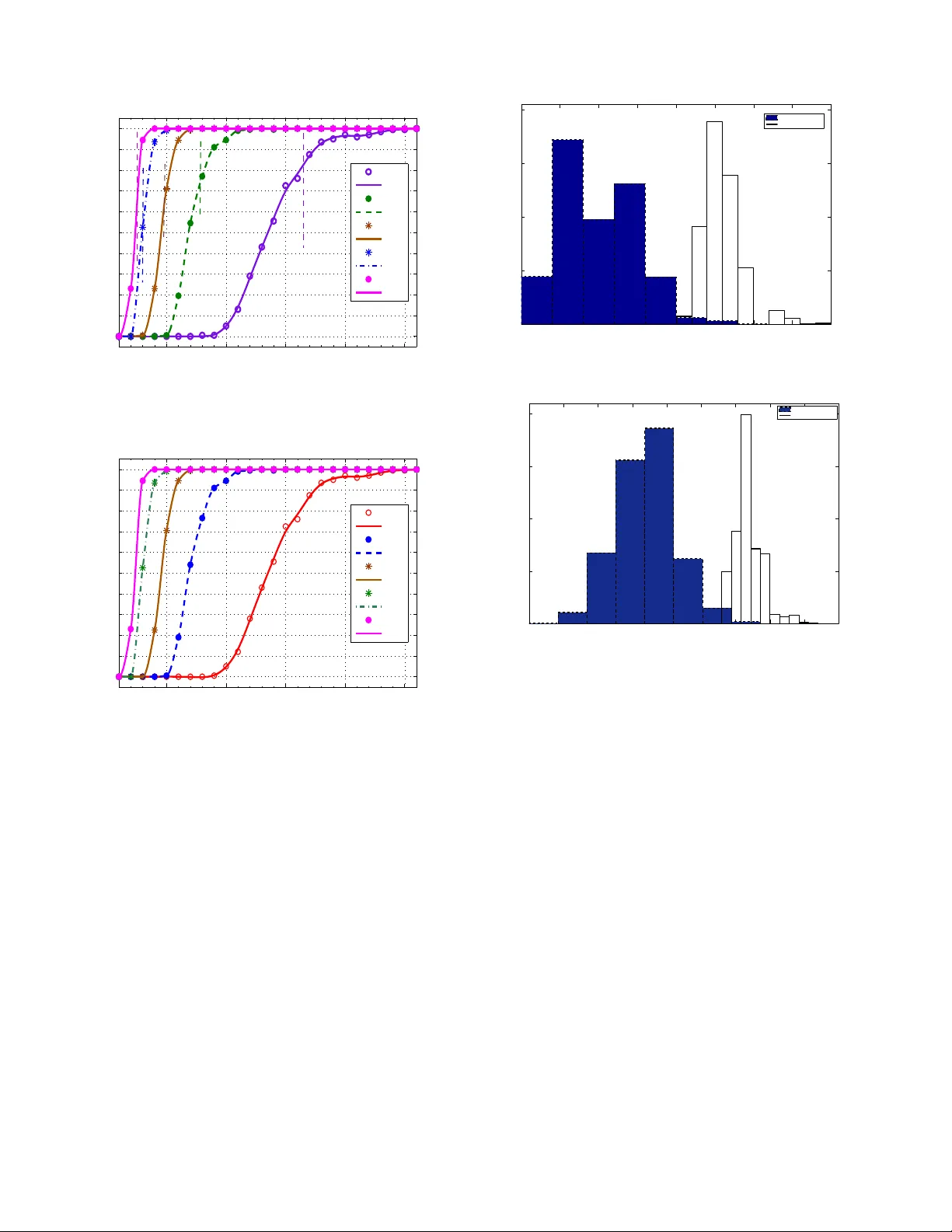
On the gradual deployment of random pairwise ke y distrib ution schemes Osman Y a ˘ gan and Armand M. Makowski Departmen t of E lectrical an d Com puter En gineerin g and the Institute for System s Research University of Marylan d, College Park College Park, M aryland 20742 oyagan@umd .edu, armand@isr .umd.ed u Abstract — In the context of wireless sensor networks, the pairwise key distribu tion scheme of Chan et a l. has several advantages over other key distribution schemes including the original scheme of Eschenauer and Gligor . However , this offline pa irwise k ey distribution mecha nism r e quires that the net work s ize be set in advance, and in volves all sensor nodes simultaneously . Here, we addr e ss this issue by describing an implementation of the pa irwise scheme that supports the gradual deployment of sensor nodes in several consecutive phases. W e discuss the key ring size needed t o maintain the secure co nnectivity throughout all the deployment phases. In particular we show that the number of keys at each sensor node can be taken to be O (log n ) in order to achieve secure connectivity ( with high probability). Keywords: W ireless sen sor network s, Secur ity , Key p redis- tribution, Random key graphs, Co nnectivity . I . I N T RO D U C T I O N W ireless sensor networks (WSNs) are distributed collections of sensors with limited cap abilities for c omputatio ns and wire- less commu nications. Such networks will likely be d eployed in h ostile environments where cryp tograph ic protection will be needed to enab le secure com municatio ns, sensor-capture detection, key r ev oc ation a nd sensor disabling . Ho wev er , tra- ditional key exch ange and d istribution protoc ols b ased o n trusting th ird p arties h av e been fo und inad equate for large- scale WSNs, e.g ., see [6], [10], [1 2] for discussions of some of th e challenges. Rando m key predistribution sche mes wer e rece ntly pro - posed to add ress so me of these challen ges. Th e idea of ran- domly assigning secu re keys to sensor nodes p rior to network deployment was first propo sed by Eschenauer and Gligor [6]. The mode ling and p erfor mance of the EG sche me, a s we refer to it h ereafter, has bee n extensiv ely investigated [1], [4], [6], [11], [13], [14], [ 15], with most of the focu s b eing on the full visibility case where nod es are all within commu nication range of each other . Under full visibility , the EG scheme in duces so- called r a ndom key graphs [1 3] ( also kno wn in the literature as uniform rand om intersection graphs [ 1]). Cond itions o n the graph param eters to ensu re the absence o f isolated n odes have been o btained indepen dently in [1], [ 13] while th e pap ers [1], [ 4], [11], [14], [15] ar e concerned with zero-o ne laws for connectivity . Alth ough the assumption of full visibility does away with th e wireless natu re of th e comm unication infrastructu re suppor ting WSNs, in return this s implification makes it possible to fo cus on how random izing the key selections affects th e establishmen t of a secure network; the connectivity results for the under lying rando m key gra ph th en provide helpf ul (thoug h optimistic) guid elines to d imension the EG scheme. The work of Esche nauer and Gligor has spu rred th e de- velopment of o ther key distribution schemes which perform better than the E G scheme in so me aspects, e.g ., [3], [5], [ 10], [12]. Althoug h these schemes somewhat improve resiliency , they fail to provide perfect resiliency again st no de c apture attacks. More importan tly , they do not provid e a n ode with the ability to authenticate the identity o f th e neighbors with which it commun icates. Th is is a major drawback in term s of network secu rity since node-to-n ode authen tication may help detect no de m isbehavior , an d p rovides resistance against n ode replication a ttacks [3]. T o addr ess this issue Chan et al. [3] have p roposed th e following random pairwise key predistribution scheme : Before deployment, each o f the n sensor nodes is paired ( offline) with K d istinct no des which are rand omly selected a mongst a ll other n − 1 no des. For each suc h pairing, a u nique pairwise key is gener ated and stored in the mem ory module s of each of the paired sensors along with the id of the other node. A secure link ca n then be established between two communic ating nodes if at least o ne of them has been assigned to the other, i.e., if th ey hav e at least on e key in commo n. See Section I I for implementation details. This sch eme h as the fo llowing advantages over the EG scheme (an d others): (i) Even if some nodes are captured, the secrecy o f the remaining node s is perfectly preserved; and (ii) Unlike earlier schem es, this scheme ena bles both nod e- to-nod e authentication and quoru m-based rev ocation withou t in volving a base station. Given these ad vantages, we foun d it of interest to model the pairwise scheme of Chan et al. and to assess its perf ormance . In [16] we began a formal in vestigation along these lines. Let H ( n ; K ) deno te the random graph on the vertex set { 1 , . . . , n } where distinct node s i and j are a djacent if they have a pairw ise key in co mmon ; a s in 2 earlier work on the EG scheme this co rrespon ds to modeling the rando m pairwise distribution scheme under full v isibility . In [16] we sh owed that th e pro bability of H ( n ; K ) being connected app roaches 1 (resp. 0 ) as n gr ows large if K ≥ 2 (resp. if K = 1 ), i.e., H ( n ; K ) is asymptotically almo st surely (a.a.s.) connected whenever K ≥ 2 . In the present pape r , we co ntinue our study of con nectivity proper ties b u t from a different perspective: W e note that in many application s, the sensor node s are expected to be d e- ployed gradua lly over time . Y et, the pairwise key distribution is an offline p airing mecha nism which simultaneo usly in volves all n no des. Thus, once th e ne twork size n is set, there is no way to add more no des to the network and still r ecu rsively expand th e p airwise distribution scheme (a s is possible f or the EG scheme). However , as explain ed in Section II-B, the gradua l deployment of a large numb er of sen sor no des is nevertheless feasible from a p ractical vie wpo int. In that context we are interested in u nderstand ing ho w the param eter K needs to scale with n large in o rder to ensure that connectivity is maintain ed a.a.s. thro ughou t gr adual deployment. W e also discuss the number of keys need ed in the memory mod ule of each sensor to achieve secure connectivity at every step o f the gradual deploym ent. Since sensor nodes are expected to have very limited memory , it is cru cial for a key distribution scheme to have low memory requ irements [5]. The key contributions of the paper can be stated as follows: Let H γ ( n ; K ) denote th e subgraph of H ( n ; K ) restricted to the nodes 1 , . . . , ⌊ γ n ⌋ . W e first p resent scaling laws for the absence of isolated no des in the form of a fu ll ze ro-on e law , and use these resu lts to formulate cond itions under which H γ ( n ; K ) is a.a. s. not connected . Then, with 0 < γ 1 < γ 2 < . . . < γ ℓ < 1 , we give conditions on n , K and γ 1 so that H γ i ( n ; K ) is a.a.s. conn ected for each i = 1 , 2 , . . . , ℓ ; this correspo nds to the case wh ere the network is connec ted in each of the ℓ phases of the gradu al deployment. As with the EG schem e, these scaling co nditions can be helpf ul for dimensionin g the p airwise key distribution in the case of gradua l deployme nt. W e also discuss the r equired numb er of keys to be kept in the memory module of ea ch sensor to ac hieve secure connectivity at e very step of the gradual deployment. Since sensor nodes are expected to h av e very limited mem ory , it is cr ucial for a ke y d istribution schem e to h ave low memor y requir ements [5]. In contra st with the EG scheme (and its variants), the key rin gs pro duced by the pairwise scheme of Chan e t al. have variable size between K and K + ( n − 1) . Still, we sho w that the maximum ke y ring size is on the o rder log n with very hig h pr obability provided K = O (log n ) . Com bining with the connectivity results, we conclude that the sensor network c an maintain the a.a.s. connectivity throug h all ph ases o f the deployment when the numb er of keys to be stored in each sensor’ s memo ry is O (log n ) ; this is a key ring size co mparab le to that of the EG scheme (in realistic WSN scenarios [4]). These resu lts show that the p airwise scheme ca n also be feasible when the ne twork is deployed gradually over time. Howe ver, as with the results in [16], the ass umption of full visibility may y ield a dim ensioning of the pa irwise scheme which is too o ptimistic. T his is due to the fact that the unreliable nature of wireless links has no t been incorpor ated in the mode l. However the results ob tained in this pap er already yield a numb er of in teresting obser vations: The obtained zero- one laws differ significan tly from th e corresponding results in the single deploym ent case [16]. Thus, the gradu al deployment may hav e a significant im pact on the dimensioning of the pairwise distribution algorithm. Y et, th e required number of keys to achieve secu re conne ctivity being O (log n ) , it is still feasible to use the p airwise scheme in th e case of grad ual deployment; the required key rin g size in EG sch eme is also O (log n ) u nder f ull-visibility [4 ]. I I . T H E M O D E L A. Implementing pairwise ke y distribution schemes The random pairwise key pred istribution scheme of Chan et al. is parametrized by two positiv e in tegers n an d K su ch that K < n . There ar e n nod es which ar e labelled i = 1 , . . . , n . with unique ids Id 1 , . . . , Id n . Write N := { 1 , . . . n } an d set N − i := N − { i } for each i = 1 , . . . , n . W ith n ode i we associate a subset Γ n,i nodes selected at rand om fro m N − i – W e say that each of the no des in Γ n,i is pa ired to nod e i . Thus, for any sub set A ⊆ N − i , we req uire P [Γ n,i = A ] =     n − 1 K  − 1 if | A | = K 0 otherwise. The selection of Γ n,i is do ne uniformly am ongst all sub sets of N − i which are o f size exactly K . The rvs Γ n, 1 , . . . , Γ n,n are assumed to be mutually in depend ent so th at P [Γ n,i = A i , i = 1 , . . . , n ] = n Y i =1 P [Γ n,i = A i ] for ar bitrary A 1 , . . . , A n subsets of N − 1 , . . . , N − n , re spec- ti vely . On the b asis of this offline r andom pairing, w e no w construct the key rin gs Σ n, 1 , . . . , Σ n,n , one f or ea ch no de, as follows: Assumed av ailab le is a collection of nK distinct cryptograp hic keys { ω i | ℓ , i = 1 , . . . , n ; ℓ = 1 , . . . , K } – These keys are drawn from a very large po ol of keys; in practice th e pool size is assumed to be muc h larger than nK , and can be safely taken to be infinite for the purpose of our d iscussion. Now , fix i = 1 , . . . , n and let ℓ n,i : Γ n,i → { 1 , . . . , K } denote a labeling of Γ n,i . For each node j in Γ n,i paired to i , the cryp tograp hic key ω i | ℓ n,i ( j ) is associated with j . For instance, if th e rand om set Γ n,i is realized as { j 1 , . . . , j K } with 1 ≤ j 1 < . . . < j K ≤ n , the n an obvious lab eling consists in ℓ n,i ( j k ) = k for each k = 1 , . . . , K with key ω i | k associated with node j k . Of course other labeling are possible. e.g., acco rding to decreasing labels or according to a ran dom permutatio n. The p airwise key ω ⋆ n,ij = [Id i | Id j | ω i | ℓ n,i ( j ) ] is constructed and inserted in th e memory modules of both nodes i an d j . Inh erent to this construction is the fact that the 3 key ω ⋆ n,ij is assigned exclusively to the pair of no des i and j , hence the termino logy p airwise distribution schem e. The ke y ring Σ n,i of n ode i is the set Σ n,i := { ω ⋆ n,ij , j ∈ Γ n,i } ∪ { ω ⋆ n,j i , i ∈ Γ n,j } (1) as we take in to account the possibility that node i was paired to some other node j . As mentioned earlier , u nder full v isibility , two no de, say i and j , can establish a secure link if at least one o f the events i ∈ Γ n,j or j ∈ Γ n,j is takin g place. Note that bo th ev ents can take pla ce, in which c ase th e memory modules of node i and j each con tain th e distinct keys ω ⋆ n,ij and ω ⋆ n,j i . I t is also plain that by constru ction this schem e supports n ode-to- node authentication . B. Gradual deploymen t Initially n node identities were generated and the ke y rin gs Σ n, 1 , . . . , Σ n,n were constructed as indicated above – Here n stands fo r the maximum po ssible network size and should be selected large enough. This key selection proced ure doe s not require the phy sical presence of the sensor entities and can be implem ented comp letely o n the software level. W e now describe how this o ffline pairw ise key d istribution scheme can support gradua l network deployment in c onsecutive stages. In the initial phase of de ployment, with 0 < γ 1 < 1 , let ⌊ γ 1 n ⌋ sensors be produced and given the labels 1 , . . . , ⌊ γ 1 n ⌋ . The key r ings Σ n, 1 , . . . , Σ n, ⌊ γ 1 n ⌋ are then inserted in to the memo ry modules of th e sensors 1 , . . . , ⌊ γ 1 n ⌋ , respec ti vely . Im agine now that more sensors are n eeded, say ⌊ γ 2 n ⌋ − ⌊ γ 1 n ⌋ sensors with 0 < γ 1 < γ 2 ≤ 1 . Then, ⌊ γ 2 n ⌋ − ⌊ γ 1 n ⌋ additional sensors would be pro duced, this second batch of sen sors would be assign ed labe ls ⌊ γ 1 n ⌋ + 1 , . . . , ⌊ γ 2 n ⌋ , and the key rings Σ n, ⌊ γ 1 n ⌋ +1 , . . . , Σ n, ⌊ γ 2 n ⌋ would be in serted into their memory modules. Once this is done , these ⌊ γ 2 n ⌋ − ⌊ γ 1 n ⌋ new sensors ar e added to the network (which n ow comprises ⌊ γ 2 n ⌋ deployed sensors). Th is step may be repeated a nu mber times: In fact, for some finite integer ℓ , consider positive scalars 0 < γ 1 < . . . < γ ℓ ≤ 1 (with γ 0 = 0 by c onv ention). W e can then dep loy the sensor network in ℓ co nsecutive p hases, with the k th phase ad ding ⌊ γ k n ⌋ − ⌊ γ k − 1 n ⌋ new no des to the network for each k = 1 , . . . , ℓ . I I I . R E L A T E D W O R K The pairwise distribution sche me naturally giv es rise to the following class o f random graphs: W ith n = 2 , 3 , . . . and positive integer K with K < n , the distinct nod es i and j are said to be adjacent , written i ∼ j , if and only if they h av e at least one key in common in their key rings, nam ely i ∼ j iff Σ n,i ∩ Σ n,j 6 = ∅ . (2) Let H ( n ; K ) de note the undirected ran dom graph on the vertex set { 1 , . . . , n } induced throu gh the adjace ncy no tion (2). W ith P ( n ; K ) := P [ H ( n ; K ) is conn ected ] , we have shown [16] the following zero-one law . Theor em 3.1 : W ith K a positi ve integer , it holds that lim n →∞ P ( n ; K ) =  0 if K = 1 1 if K ≥ 2 . (3) Moreover , f or any K ≥ 2 , we have P ( n ; K ) ≥ 1 − 27 2 n 2 (4) for all n = 2 , 3 , . . . sufficiently large. I V . T H E R E S U LT S W e now presen t the main results of the paper . W e start with the results regarding the ke y r ing sizes: Theorem 3 .1 shows that very small values of K suffice for a.a. s. conn ectivity of the rand om graph H ( n ; K ) . The mere fact that H ( n ; K ) becomes connec ted even with very small K values do es n ot imply th at the numb er o f ke y s (i.e., the size | Σ n,i | ) to ach iev e connectivity is n ecessarily small. Th is is becau se in contrast with the EG scheme and its variants, the pairwise scheme produ ces key rings of variable size between K an d K + ( n − 1) . T o e xplore this issue furth er we first obtain minimal conditio ns on a scalin g K : N 0 → N 0 which ensure that the ke y ring of a node has size roughly of the order (o f its mean) 2 K n when n is large. Lemma 4 .1: For any scaling K : N 0 → N 0 , we have | Σ n, 1 ( K n ) | 2 K n P → n 1 (5) as soon as lim n →∞ K n = ∞ . Thus, when n is large | Σ n, 1 ( K n ) | fluctuates from K n to K n + ( n − 1) with a propensity to hover ab out 2 K n under th e condition s o f Lemma 4.1. This result is sharpened with th e help of a concentr ation r esult for th e maximal key ring s ize under an appropr iate class of scalings. W e define the maximal key ring size by M n :=  max i =1 ,...,n | Σ n,i |  , n = 2 , 3 , . . . Theor em 4.2 : Consider a scaling K : N 0 → N 0 of the form K n ∼ λ log n (6) with λ > 0 . If λ > λ ⋆ := (2 log 2 − 1) − 1 ≃ 2 . 6 , then there exists c ( λ ) in the interval (0 , λ ) such that lim n →∞ P [ | M n ( K n ) − 2 K n | ≥ c log n ] = 0 (7) whenever c ( λ ) < c < λ . In th e course of proving Theo rem 4.2 we also show that P [ | M n ( K n ) − 2 K n | ≥ c log n ] ≤ 2 n − h ( γ ; c ) (8) for all n = 1 , 2 , . . . whenever c ( γ ) < c < γ with h ( γ ; c ) > 0 specified in [16]. W ith the network dep loyed gradu ally over time as describ ed in Section II, we are now in terested in understanding how th e parameter K needs to be scaled with large n to ensur e that connectivity is maintained a.a.s. througho ut gra dual deploy- ment. Con sider positive integers n = 2 , 3 , . . . an d K with K < n . Wit h γ in the inter val (0 , 1 ) , let H γ ( n ; K ) d enote the subgrap h of H ( n ; K ) r estricted to the nod es { 1 , . . . , ⌊ γ n ⌋} . Giv en scalar s 0 < γ 1 < . . . < γ ℓ ≤ 1 , we seek co nditions on the parame ters K and n such that H γ i ( n ; K ) is a. a.s. connected fo r each i = 1 , 2 , . . . , ℓ . 4 First we write P γ ( n ; K ) := P [ H γ ( n ; K ) is conn ected ] = P [ C n,γ ( K )] with C n,γ ( K ) deno ting the event that H γ ( n ; K ) is con nected. The fact that H ( n ; K ) is connected does no t imply that H γ ( n ; K ) is necessarily co nnected. Ind eed, with distinct node s i, j = 1 , . . . , ⌊ γ n ⌋ , the path tha t exists in H ( n ; K ) between these nodes (as a result of the assum ed connectivity of H ( n ; K ) ) m ay comprise edges that are not in H γ ( n ; K ) . The next result provides an analog of Th eorem 3.1 in this new setting. Theor em 4.3 : W ith γ in the u nit interval (0 , 1) and c > 0 , consider a scaling K : N 0 → N 0 such that K n ∼ c log n γ . (9) Then, we have lim n →∞ P γ ( n ; K n ) = 1 whenever c > 1 . The random graphs H ( n ; K ) and H γ ( n ; K ) h ave very dif- ferent neighb orhoo d structures. In deed, any n ode in H ( n ; K ) has degree at least K , so that no node is isolated in H ( n ; K ) . Ho wever , there is a positi ve probability that iso- lated no des exist in H γ ( n ; K ) . In fact, with P ⋆ γ ( n ; K n ) := P [ H γ ( n ; K ) con tains no isolated n odes ] , we have the follow- ing z ero-on e law . Theor em 4.4 : W ith γ in the unit in terval (0 , 1) , consider a scaling K : N 0 → N 0 such that ( 9) holds fo r some c > 0 . Then, we have lim n →∞ P ⋆ γ ( n ; K n ) =  0 if c < r ( γ ) 1 if c > r ( γ ) (10) where the threshold r ( γ ) is giv en by r ( γ ) :=  1 − log(1 − γ ) γ  − 1 . (11) It is easy to check that r ( γ ) is decreasin g on th e interv a l [0 , 1 ] with lim γ ↓ 0 r ( γ ) = 1 2 and lim γ ↑ 1 r ( γ ) = 0 . Since a connected grap h has no isolated nodes, Th eorem 4.4 yield s lim n →∞ P [ H γ ( n ; K n ) is connected] = 0 if the scalin g K : N 0 → N 0 satisfies (9) with c < r ( γ ) . The following co rollary is n ow immediate from Theo rem 4.3. Cor ollary 4.5: W ith γ in the un it inter val (0 , 1) , consider a scaling K : N 0 → N 0 such that (9) ho lds for some c > 0 . Then, with r ( γ ) giv en by (11), we ha ve lim n →∞ P γ ( n ; K n ) =  0 if c < r ( γ ) 1 if c > 1 (12) Corollary 4 .5 does not p rovide a f ull zero -one law for the connectivity of H γ ( n ; K n ) as there is a gap be tween the threshold r ( γ ) of the zero -law and the thresh old 1 of the on e- law . Y et, the gap between the thresh olds of the zero- law and the one- law is qu ite small with 1 2 < 1 − r ( γ ) < 1 . Mo re importan tly , Corollary 4.5 alr eady implies (v ia a mon otonicity argument) th at it is necessary and sufficient to keep the parameter K n on th e ord er of log n to ensure that the grap h H γ ( n ; K n ) is a.a.s. con nected. It is worth pointing out that the simu lation results in Section V sug gest the existence of a full zero-o ne law for P γ ( n ; K n ) with a thresho ld resembling r ( γ ) . This would not be sur prising sin ce in many known classes of r andom g raphs, the absence of isolated nod es and graph connectivity are asymp totically equ iv alent properties, e.g., Erd ˝ os-R ´ enyi graphs [2] and random key graphs [11], among others. Finally we turn to g radual n etwork deployment as discussed in Section II. Theor em 4.6 : W ith 0 < γ 1 < γ 2 < . . . < γ ℓ ≤ 1 , co nsider a scaling K : N 0 → N 0 such that K n ∼ c log n γ 1 (13) for some c > 1 . Then we hav e lim n →∞ P [ C n,γ 1 ( K n ) ∩ . . . ∩ C n,γ ℓ ( K n )] = 1 . (14) The event [ C γ 1 ,n ( K n ) ∩ . . . ∩ C γ ℓ ,n ( K n )] corresp onds to the network in each o f its ℓ ph ases being connected as more nodes get add ed – In other words, on that event the sen sors do form a co nnected network at each phase of deployment. As a result, we infer v ia Th eorem 4 .6 th at the co ndition ( 13) (with c > 1 ) is enou gh to ensure that the ne twork remains a.a.s. co nnected as mor e sensor s are deployed over time. The main c onclusion s of the pap er , obtained by combining Theorem 4.2 an d Theor em 4.6, can now be summar ized as follows: Cor ollary 4.7: W ith 0 < γ 1 < γ 2 < . . . < γ ℓ ≤ 1 , consider a scaling K : N 0 → N 0 such that K n = O (lo g n ) with K n ≥ max  ( γ 1 ) − 1 , λ ⋆  · log n, n = 2 , 3 , . . . Then, the following holds: 1) The maximum numb er of ke ys kept in the mem ory mod- ule of each sensor will be a.a.s. less than 3 K n ; 2) The network dep loyed gradually in ℓ steps (as in Section II) will be a.a.s. connected in each of the ℓ phases of deployment. V . S I M U L AT I O N S T U DY W e now present experim ental r esults in support of the theoretical finding s. I n each set of experime nts, we fix n and γ . Then , we generate rand om graphs H γ ( n ; K ) f or each K = 1 , . . . , K max where the maximal value K max is selected large enou gh. In e ach case, we ch eck whether the gen erated random graph has isolated nodes and is connected . W e repeat the pro cess 20 0 times for each p air of values γ and K in order to estimate the pro babilities of the events of in terest. For v ario us v alues of γ , Figure 1(a) depic ts the estimated probab ility P ⋆ γ ( n ; K ) that H γ ( n ; K ) has no isolated nodes as a fu nction of K . Here, n is taken to be 1 , 000 . T he plots in Figure 1(a) clearly confirm the claims o f Theorem 4.4: In each case P ⋆ γ ( n ; K ) exhibits a thresho ld behavior and th e transitions f rom P ⋆ γ ( n ; K ) = 0 to P ⋆ γ ( n ; K ) = 1 tak e p lace around K = r ( γ ) log n γ as dictated by Theorem 4.4; the critical value K = r ( γ ) log n γ is shown by a v ertical dashed line in each plot. 5 5 10 15 20 25 0 0.1 0.2 0.3 0.4 0.5 0.6 0.7 0.8 0.9 1 K Prob that H γ (n;K) has no isolated nodes γ =0.2 γ =0.4 γ =0.6 γ =0.8 γ =0.9 (a) 5 10 15 20 25 0 0.1 0.2 0.3 0.4 0.5 0.6 0.7 0.8 0.9 1 K Prob that H γ (n;K) is connected γ =0.2 γ =0.4 γ =0.6 γ =0.8 γ =0.9 (b) Fig. 1. a ) Probabil ity that H γ ( n ; K ) contai ns no isolated for n = 1000 ; in each case, the e mpirical proba bilit y valu e is o btaine d through 200 expe riments. V ertical dashed lines stand for the criti cal thresholds asserted by T heorem 4.4. It is cl ear t hat the th eoreti cal findings a re in pe rfect a greement with th e p racti cal observ ations. b ) Probabil ity that H γ ( n ; K ) is connecte d for n = 1 , 000 obtaine d in the same way . Clea rly , the curv es are a lmost indist inguishab le from the correspondi ng ones of part ( a ) ; this supports the claim that absence of isolate d nodes and connecti vity are asymptotica lly equi val ent propert ies. Similarly , Figure 1(b) shows the estimated pro bability P γ ( n ; K ) v .s. K for various values of γ with n = 1000 . For each specified γ , we see that the variation of P γ ( n ; K ) with K is almost indistinguishable fr om that of P ⋆ γ ( n ; K ) supp orting the claim that P γ ( n ; K ) exhib its a full ze ro-on e law similar to that of Theo rem 4 .4 with a thresho ld behaving like r ( γ ) . W e can also co nclude by mono tonicity that P γ ( n ; K ) = 1 whenever (9) h olds with c > 1 ; this verifies Theore m 4.3. Furthermo re, it is evident fr om Figure 1(b) tha t f or a given K and n , P γ ( n ; K ) increases as γ increases suppo rting Th eorem 4.6. W e also present experimental results that validate Lemma 4.1 and T heorem 4 .2: For fixed values o f n and K we have 4 6 8 10 12 14 16 18 20 %0 %10 %20 %30 %40 Key ring size Frequency of occurrence n=200, K=4 All key rings Largest key ring of n nodes (a) 25 30 35 40 45 50 55 60 65 70 %0 %10 %20 %30 %40 Key ring size Frequency of occurrence n=500, K=21 All key rings Largest key ring of n nodes (b) Fig. 2. a ) Ke y ring sizes observed in 1 , 000 expe riments for n = 200 and K = 4 – Only 2% of the key rings are larger than 3 K and the largest ke y ring has size 20 . b ) Ke y ring sizes observe d in 1 , 000 expe riments for n = 500 and K = 21 – Out of the 500 , 000 ke y rings prod uced o nly 9 happene d to be lar ger than 3 K while the larg est size observed is 67 . constructed key rings acco rding to the mechanism p resented in Section I I. For each pair of parameters n and K , the ex- periments ha ve been repeated 1 , 000 times yielding 1 , 000 × n key rings for each parameter pair . The r esults a re d epicted in Figures 1-4 which sho w th e ke y ring sizes acco rding to th eir frequen cy of occurren ce. The histog rams in blue consider all of the prod uced 1 , 000 × n ke y rings, while the histogr ams in white consider only the 1 , 00 0 maximal key rin g sizes, i.e., only the largest key r ing a mong n nodes in an experiment. It is immediate from F igures 2(a)-3(b) that the ke y ring sizes tend to conc entrate aroun d 2 K , validating the claim o f Lemma 4.1. As would be expected, th is concentra tion beco mes more evident as n gets large. It is also clear that, in almost all cases the ma ximum size of a key ring (out of n no des) is less than 3 K v alid ating the claim of Theo rem 4.2. 6 25 30 35 40 45 50 55 60 65 70 75 %0 %10 %20 %30 %40 Key ring size Frequency of occurrence n=1000, K=24 All key rings Largest key ring of n nodes (a) 30 35 40 45 50 55 60 65 70 75 80 %0 %10 %20 %30 %40 Key ring size Frequency of occurrence n=2000, K=26 All key rings Largest key ring of n nodes (b) Fig. 3. a ) Ke y ring sizes observed in 1 , 000 expe riments for n = 1 , 000 and K = 24 – 1 , 000 , 000 ke y rings are produced. Only 5 of them happened to be larger than 3 K and the largest observ ed ke y ring size is 75 . b ) Ke y ring sizes observ ed in 1 , 000 expe riments for n = 2 , 000 and K = 26 – Out of the 2000000 key rings produced only 2 happene d to be lar ger than 3 K the largest of them ha ving 80 ke ys. V I . C O N C L U S I O N In this paper, we co nsider th e pairwise key distribution scheme of Chan et al. which w as proposed to establish s ecurity in wireless sensor networks. This pairwise schem e has many advantages over other key distribution s chemes b ut deemed not scalable due to i ) large number of ke ys requir ed to establish se- cure conn ectivity and i i ) the difficulties in the im plementatio n when sensors are r equired to be deployed in mu ltiple stages. Here, we ad dress this issue and propo se an implementation of the pairwise scheme tha t supports the grad ual d eployment of sensor nodes in several con secutiv e phases. W e show how should the sch eme param eter be adjusted w ith the nu mber n of sensors so th at th e secure co nnectivity can be maintain ed in the network througho ut all stages of the deployment. W e also exp lore the relation b etween th e sch eme parameter and the amount of memo ry that each sensor nee ds to spare for storing secure keys. By showing th at the req uired number of keys is O (log n ) to achie ve con nectivity at every step of th e deployment, we confirm the scalab ility of the pairwise scheme in the context of WSNs. V I I . A P R O O F O F T H E O R E M 4 . 3 Fix n = 2 , 3 , . . . and γ in the inter val (0 , 1) , and c onsider a positive integer K ≥ 2 . Throu ghou t the d iscussion, n is sufficiently large so that the cond itions 2( K + 1) < n , K + 1 ≤ n − ⌊ γ n ⌋ a nd 2 < γ n (15) are all enf orced; these co nditions are mad e in or der to av oid degenerate situations which ha ve no bearing on the final result. There is n o loss of genera lity in doing so as we e ventua lly let n go to infinity . For any non-empty s ubset R c ontained in { 1 , . . . , ⌊ γ n ⌋} , we define the graph H γ ( n ; K )( R ) (with vertex set R ) as the subgrap h of H γ ( n ; K ) restricted to the nodes in R . W e say that R is isolated in H γ ( n ; K ) if there ar e no ed ges (in H γ ( n ; K ) ) between the nodes in R and the nod es in its co mplemen t R c | γ := { 1 , . . . , ⌊ γ n ⌋} − R . This is characterized by th e event B n,γ ( K ; R ) given by B n,γ ( K ; R ) := h i 6∈ Γ n,j , j / ∈ Γ n,i , i ∈ R, j ∈ R c | γ i . Also, let C n,γ ( K ; R ) den ote the event that the indu ced su b- graph H γ ( n ; K )( R ) is itself connected . Finally , we set A n,γ ( K ; R ) := C n,γ ( K ; R ) ∩ B n,γ ( K ; R ) . The discussion starts with the following basic observation: If H γ ( n ; K ) is not conn ected, then there must exist a non- empty subset R of nodes co ntained in { 1 , . . . , ⌊ γ n ⌋} , such that H γ ( n ; K )( R ) is itself con nected while R is isolated in H γ ( n ; K ) . This is captured by the in clusion C n,γ ( K ) c ⊆ ∪ R ∈N n,γ A n,γ ( K ; R ) (16) with N n,γ denoting the collection of all no n-empty subsets of { 1 , . . . , ⌊ γ n ⌋} . This un ion n eed o nly b e taken over all non - empty subsets R of { 1 , . . . , ⌊ γ n ⌋} with 1 ≤ | R | ≤ ⌊ ⌊ γ n ⌋ 2 ⌋ , and it is u seful to note th at ⌊ ⌊ γ n ⌋ 2 ⌋ = ⌊ γ n 2 ⌋ . Th en, a standard union b ound argument immediately g i ves P [ C n,γ ( K ) c ] ≤ X R ∈N n,γ : 1 ≤| R |≤⌊ γ n 2 ⌋ P [ A n,γ ( K ; R )] = ⌊ γ n 2 ⌋ X r =1   X R ∈N n,γ ,r P [ A n,γ ( K ; R )]   (17) where N n,γ ,r denotes the collection of all subsets of { 1 , . . . , ⌊ γ n ⌋} with exactly r elements. For each r = 1 , . . . , ⌊ γ n ⌋ , when R = { 1 , . . . , r } , we simplify the no tation by writing A n,γ ,r ( K ) := A n,γ ( K ; R ) , B n,γ ,r ( K ) := B n,γ ( K ; R ) an d C n,γ ,r ( K ) := C n,γ ( K ; R ) . For r = ⌊ γ n ⌋ , the notatio n C n,γ , ⌊ γ n ⌋ ( K ) coincid es with C n,γ ( K ) as defin ed earlier . Und er the enforced assump tions, it is a simple m atter to check by exchan geability that P [ A n,γ ( K ; R )] = P [ A n,γ ,r ( K )] , R ∈ N n.γ ,r 7 and the expression X R ∈N γ ,r P [ A n,γ ( K ; R )] =  ⌊ γ n ⌋ r  P [ A n,γ ,r ( K )] follows since |N n,γ ,r | =  ⌊ γ n ⌋ r  . Substituting in to ( 17) we obtain the bou nds P [ C n,γ ( K ) c ] ≤ ⌊ γ n 2 ⌋ X r =1  ⌊ γ n ⌋ r  P [ B n,γ ,r ( K )] (18) as we make u se of the obvious inclusion A n,γ ,r ( K ) ⊆ B n,γ ,r ( K ) . Under the en forced assump tions, we get P [ B n,γ ,r ( K )] (19) =  n −⌊ γ n ⌋ + r − 1 K   n − 1 K  ! r ·  n − r − 1 K   n − 1 K  ! ⌊ γ n ⌋− r . T o see why this last relation hold s, recall that for the set { 1 , . . . , r } to be isolate d in H γ ( n ; K ) we need th at (i) each o f the nodes r + 1 , . . . , ⌊ γ n ⌋ are adjacent o nly to no des ou tside the set of nod es { 1 , . . . , r } ; and (ii) none of the nodes 1 , . . . , r are adjacent with any of th e nodes r + 1 , . . . , ⌊ γ n ⌋ – This last requirem ent does not preclud e adjacency with any of the nodes ⌊ γ n ⌋ + 1 , . . . , n . Repo rting (1 9) into (18), we c onclude that P [ C n,γ ( K ) c ] (20) ≤ ⌊ γ n 2 ⌋ X r =1  ⌊ γ n ⌋ r   n −⌊ γ n ⌋ + r − 1 K   n − 1 K  ! r ·  n − r − 1 K   n − 1 K  ! ⌊ γ n ⌋− r with cond itions (15) ensuring that the bin omial coefficients are well defined. The remaind er of the proof consists in bou nding each of the terms in ( 20). T o do so we m ake use of several standard bound s. First we recall the well-known bound  ⌊ γ n ⌋ r  ≤  ⌊ γ n ⌋ e r  r , r = 1 , . . . , ⌊ γ n ⌋ . Next, for 0 ≤ K ≤ x ≤ y , we note that  x K   y K  = K − 1 Y ℓ =0  x − ℓ y − ℓ  ≤  x y  K since x − ℓ y − ℓ decreases a s ℓ increases from ℓ = 0 to ℓ = K − 1 . Now pick r = 1 , . . . , ⌊ γ n ⌋ . Under (15) we can ap ply these bound s to obtain  ⌊ γ n ⌋ r   n −⌊ γ n ⌋ + r − 1 K   n − 1 K  ! r ·  n − r − 1 K   n − 1 K  ! ⌊ γ n ⌋− r ≤  ⌊ γ n ⌋ e r  r ·  n − ⌊ γ n ⌋ + r − 1 n − 1  r K ×  n − r − 1 n − 1  K ( ⌊ γ n ⌋− r ) ≤  γ ne r  r  1 − ⌊ γ n ⌋ − r n − 1  r K  1 − r n − 1  K ( ⌊ γ n ⌋− r ) ≤ ( γ ne ) r ·  1 − ⌊ γ n ⌋ − r n  r K ·  1 − r n  K ( ⌊ γ n ⌋− r ) ≤ ( γ ne ) r · e − ( ⌊ γ n ⌋− r n ) r K · e − ( r n ) ( ⌊ γ n ⌋− r ) K . It is plain that P [ C n,γ ( K ) c ] ≤ ⌊ γ n 2 ⌋ X r =1 ( γ ne ) r · e − 2 ( ⌊ γ n ⌋− r n ) r K ≤ ⌊ γ n 2 ⌋ X r =1 γ ne · e − 2  ⌊ γ n ⌋− ⌊ γ n 2 ⌋ n  K ! r (21) as we note that ⌊ γ n ⌋ − r n ≥ ⌊ γ n ⌋ − ⌊ γ n 2 ⌋ n , r = 1 , . . . , ⌊ γ n 2 ⌋ . Next, co nsider a scaling K : N 0 → N 0 such that (9) hold s for some c > 1 , a nd replace K by K n in (21) according to this scaling. Using the form (9) of the scaling we g et, a n := γ ne · e − 2  ⌊ γ n ⌋− ⌊ γ n 2 ⌋ n  K n = ( γ e ) · n 1 − 2 c n  ⌊ γ n ⌋− ⌊ γ n 2 ⌋ γ n  for each n = 1 , 2 , . . . , with lim n →∞ c n = c . It is a simple matter to chec k that lim n →∞  2 c n  ⌊ γ n ⌋ − ⌊ γ n 2 ⌋ γ n  = c, so that by virtue o f the fact tha t c > 1 , we have lim n →∞ a n = 0 . (22) From (21) we conclude that P [ C n,γ ( K n ) c ] ≤ ⌊ γ n 2 ⌋ X r =1 ( a n ) r ≤ ∞ X r =1 ( a n ) r = a n 1 − a n where for n suf ficiently lar ge the summability of the geometric series is guaran teed by (22). The co nclusion lim n →∞ P [ C n,γ ( K ) c ] = 0 is n ow a straigh tforward conse- quence o f th e last bou nd, again by vir tue o f (2 2). V I I I . A P R O O F O F T H E O R E M 4 . 4 Fix n = 2 , 3 , . . . and consider γ in (0 , 1 ) and positi ve integer K s uch that K < n . W e write χ n,γ ,i ( K ) := 1 [Node i is isolated in H γ ( n ; K )] for each i = 1 , . . . , ⌊ γ n ⌋ . The numb er of isolated nodes in H γ ( n ; K ) is simply given by I n,γ ( K ) := ⌊ γ n ⌋ X i =1 χ n,γ ,i ( K ) , whence the rand om gr aph H γ ( n ; K ) has no isolated nod es if I n,γ ( K ) = 0 . The metho d of first mom ent [8, Eqn (3.10 ), p . 55] and seco nd momen t [8, Remark 3.1 , p. 55] yield the useful bound s 1 − E [ I n,γ ( K )] ≤ P [ I n,γ ( K ) = 0] ≤ 1 − E [ I n,γ ( K )] 2 E [ I n,γ ( K ) 2 ] . (23) 8 The rvs χ n,γ , 1 ( K ) , . . . , χ n,γ , ⌊ γ n ⌋ ( K ) being excha ngeable, we find E [ I n,γ ( K )] = ⌊ γ n ⌋ E [ χ n,γ , 1 ( K )] (24) and E  I n,γ ( K ) 2  = ⌊ γ n ⌋ E [ χ n,γ , 1 ( K )] (25) + ⌊ γ n ⌋ ( ⌊ γ n ⌋ − 1) E [ χ n,γ , 1 ( K ) χ n,γ , 2 ( K )] by th e b inary nature of the rv s inv olved. It then f ollows in the usual m anner th at E  I n,γ ( K ) 2  E [ I n,γ ( K )] 2 = 1 ⌊ γ n ⌋ E [ χ n,γ , 1 ( K )] (26) + ⌊ γ n ⌋ − 1 ⌊ γ n ⌋ E [ χ n,γ , 1 ( K ) χ n,γ , 2 ( K )] ( E [ χ n,γ , 1 ( K )]) 2 . From (23) and (24) we conclu de th at the one- law lim n →∞ P [ I n,γ ( K n ) = 0] = 1 h olds if we show that lim n →∞ ⌊ γ n ⌋ E [ χ n,γ , 1 ( K n )] = 0 . (27) On th e o ther ha nd, it is plain from (23) and (26) that the zero-law lim n →∞ P [ I n,γ ( K n ) = 0] = 0 will be established if lim n →∞ ⌊ γ n ⌋ E [ χ n, 1 ( K n )] = ∞ (28) and lim sup n →∞ E [ χ n,γ , 1 ( K n ) χ n,γ , 2 ( K n )] ( E [ χ n,γ , 1 ( K n )]) 2 ! ≤ 1 . (29) The next two techn ical lem mas establish (2 7), (28) and (29) under the app ropriate cond itions o n the scaling K : N 0 → N 0 . Lemma 8 .1: Consider γ in (0 , 1) and a scaling K : N 0 → N 0 such that (9) holds for some c > 0 . W e have lim n →∞ n E [ χ n,γ , 1 ( K n )] =    0 if c > r ( γ ) ∞ if c < r ( γ ) (30) with r ( γ ) specified via (11). Lemma 8 .2: Consider γ in (0 , 1) and a scaling K : N 0 → N 0 such that (9) holds for some c > 0 . W e have lim sup n →∞ E [ χ n,γ , 1 ( K n ) χ n,γ , 2 ( K n )] ( E [ χ n,γ , 1 ( K n )]) 2 ! ≤ 1 . (31) Proofs of L emma 8.1 and Lemm a 8. 2 can be foun d in Section VIII -A and Section VIII- B, respectively . T o complete the proof of Theorem 4.4, pick a scalin g K : N 0 → N 0 such that (9) ho lds for some c > 0 . Under the con dition c > r ( γ ) we get (27) fr om Lemma 8.1 and the one-law lim n →∞ P [ I n,γ ( K n ) = 0] = 1 follows. Next, assume the condition c < r ( γ ) . W e obtain (28) and (29) with the help of L emmas 8.1 and 8. 2, r espectively , and the co nclusion lim n →∞ P [ I n,γ ( K n ) = 0] = 0 is now immediate. A. A pr oof o f Lemma 8.1 Fix n = 2 , 3 , . . . and γ in (0 , 1) , and consider a positi ve integer K such that K < n . Here as well there is n o loss of generality in assuming n − ⌊ γ n ⌋ ≥ K and ⌊ γ n ⌋ > 1 . Unde r the en forced assumptions, we get E [ χ n,γ , 1 ( K )] =  n −⌊ γ n ⌋ K   n − 1 K   n − 2 K   n − 1 K  ! ⌊ γ n ⌋− 1 = a ( n ; K ) ·  1 − K n − 1  ⌊ γ n ⌋− 1 (32) with a ( n ; K ) := ( n − ⌊ γ n ⌋ )! ( n − ⌊ γ n ⌋ − K )! · ( n − 1 − K )! ( n − 1)! . Now pick a scaling K : N 0 → N 0 such that (9) holds for some c > 0 and replace K by K n in (32) with respect to this scaling. Applying Stirling ’ s form ula m ! ∼ √ 2 π m  m e  m ( m → ∞ ) to the factorials a ppearing in (32), we r eadily get a ( n ; K n ) ∼ s ( n − ⌊ γ n ⌋ )( n − 1 − K n ) ( n − ⌊ γ n ⌋ − K n )( n − 1) · α n β n ∼ α n β n (33) under th e en forced a ssumptions on the scaling with α n := ( n − K n − 1) n − K n − 1 ( n − 1) n − 1 =  1 − K n n − 1  n − 1 · ( n − K n − 1) − K n and β n := ( n − ⌊ γ n ⌋ ) n −⌊ γ n ⌋ ( n − ⌊ γ n ⌋ − K n ) n −⌊ γ n ⌋− K n =  1 − K n n − ⌊ γ n ⌋  − ( n −⌊ γ n ⌋ ) · ( n − ⌊ γ n ⌋ − K n ) K n . In o btaining the asymptotic behavior o f (33 ) we rely on the following technical fact: F o r any sequ ence m : N 0 → N 0 with m n = O ( n ) , we have  1 − K n m n  m n ∼ e − K n . (34) T o see why (34) holds, reca ll th e elem entary de compo sition log(1 − x ) = − x − Ψ( x ) with Ψ( x ) := Z x 0 t 1 − t dt valid for 0 ≤ x < 1 . Using this fact, we get  1 − K n m n  m n = e − K n · e − m n Ψ ( K n m n ) (35) for all n = 1 , 2 , . . . . 9 Under the enfo rced assumptions we have m n = O ( n ) an d K n = O (log n ) , so that lim n →∞ K n m n = 0 and lim n →∞ m n  K n m n  2 = 0 . It is now plain that lim n →∞ m n Ψ  K n m n  = 0 as we note that lim x ↓ 0 Ψ( x ) x 2 = 1 2 . This e stablishes (34) via (35). Using (34), first with m n = n − 1 , then with m n = n −⌊ γ n ⌋ , we obtain  1 − K n n − 1  n − 1 ∼ e − K n and  1 − K n n − ⌊ γ n ⌋  − ( n −⌊ γ n ⌋ ) ∼  e − K n  − 1 = e K n , whence α n β n ∼  n − ⌊ γ n ⌋ − K n n − K n − 1  K n . (36) W ith the help of (32) and (3 3) we now conclud e that n E [ χ n,γ , 1 ( K n )] (37) ∼ n  1 − K n n − 1  ⌊ γ n ⌋− 1 ·  n − ⌊ γ n ⌋ − K n n − K n − 1  K n . A final application o f ( 34), this tim e with m n = n − 1 , gives  1 − K n n − 1  ⌊ γ n ⌋− 1 =  1 − K n n − 1  n − 1 ! ⌊ γ n ⌋− 1 n − 1 ∼ e − ⌊ γ n ⌋− 1 n − 1 K n (38) since lim n →∞ ⌊ γ n ⌋− 1 n − 1 = γ . Reporting (38) into (3 7) we obtain n E [ χ n,γ , 1 ( K n )] ∼ e ζ n (39) with ζ n := log n −  ⌊ γ n ⌋ − 1 n − 1 + log  n − ⌊ γ n ⌋ − K n n − K n − 1  K n for all n = 1 , 2 , . . . . Finally , fr om the c ondition (9) o n the scaling, we see that lim n →∞ ζ n log n = 1 − c + c log(1 − γ ) γ = 1 − c r ( γ ) . Thus, lim n →∞ ζ n = −∞ (resp. ∞ ) if r ( γ ) > c (resp. r ( γ ) < c ) and the desired result follows upo n usin g (3 9). B. A pr oof o f Lemma 8.2 Fix positive integers n = 3 , 4 , . . . and K with K < n . With γ in (0 , 1) , we again assume that n − ⌊ γ n ⌋ ≥ K and ⌊ γ n ⌋ > 1 . It is a simple matter to check th at E [ χ n,γ , 1 ( K ) χ n,γ , 2 ( K )] =  n −⌊ γ n ⌋ K   n − 1 K  ! 2  n − 3 K   n − 1 K  ! ⌊ γ n ⌋− 2 and in voking (32) we read ily co nclude th at E [ χ n,γ , 1 ( K ) χ n,γ , 2 ( K )] ( E [ χ n,γ , 1 ( K )]) 2 =  n − 3 K   n − 1 K  ! ⌊ γ n ⌋− 2 ·  n − 1 K   n − 2 K  ! 2( ⌊ γ n ⌋− 1) =  n − 1 − K n − 1   n − 2 − K n − 2  ⌊ γ n ⌋− 2 ×  n − 1 n − 1 − K  2( ⌊ γ n ⌋− 1) =  n − 2 − K n − 2  ⌊ γ n ⌋− 2 ·  n − 1 n − 1 − K  ⌊ γ n ⌋ =  1 − K n − 2  ⌊ γ n ⌋− 2 ·  1 + K n − 1 − K  ⌊ γ n ⌋ ≤ e − K · E ( n ; K ) (40) where we have set E ( n ; K ) := ⌊ γ n ⌋ − 2 n − 2 − ⌊ γ n ⌋ n − 1 − K . Elementary calculations show that − K · E ( n ; K ) = ⌊ γ n ⌋ n − 2 · K ( K − 1) n − 1 − K + 2 K n − 2 . Now pick a scaling K : N 0 → N 0 such that (9) holds for some c > 0 . It is plain that lim n →∞ K n E ( n ; K n ) = 0 and the co nclusion ( 31) fo llows from ( 40). I X . A P R O O F O F T H E O R E M 4 . 6 Pick 0 < γ 1 < γ 2 < . . . < γ ℓ ≤ 1 an d co nsider a scalin g K : N 0 → N 0 such th at K n ∼ c log n γ 1 for some c > 1 . It is plain that ( 14) will hold provided lim n →∞ P [ C n,γ k ( K n )] = 1 , k = 1 , . . . , ℓ. (41) For each k = 1 , 2 , . . . , ℓ , we note that c log n γ 1 = c k log n γ k with c k := c γ k γ 1 for all n = 1 , 2 , . . . . But c > 1 implies c k > 1 since γ 1 < . . . < γ ℓ . As a result, H γ k ( n ; K n ) will be a.a.s. con nected by virtue of The orem 4.3 applied to H γ k ( n ; K ) , and (41) ind eed holds. 10 X . A P R O O F O F L E M M A 4 . 1 Fix n = 2 , 3 , . . . and p ositiv e integer K with K < n . For each i = 1 , 2 , . . . , n , n ode i is assigned a key r ing Σ n,i whose size is given by | Σ n,i | = | Γ n,i | + n X j =1 , j 6 = i 1 [ i ∈ Γ n,j ] . (42) This is a s imple consequen ce of the definition (1). W e also define the maxima l key ring size as M n := max i =1 ,...,n | Σ n,i | . It is easy to see that | Σ n,i | = K + B n,i (43) where B n,i is the rv determined through B n,i := n X j =1 , j 6 = i 1 [ i ∈ Γ n,j ] . Under the enforce d independ ence assumptions, the rv B n,i is a binomial rv Bin( n − 1 , K n − 1 ) , with E [ B n,i ] = ( n − 1) · K n − 1 = K and V a r [ B n,i ] = ( n − 1) · K n − 1 · n − 1 − K n − 1 . As a result, E [ | Σ n,i | ] = 2 K and V a r [ | Σ n,i | ] = K  1 − K n − 1  . It is now plain that E "     | Σ n,i | E [ | Σ n,i | ] − 1     2 # = V a r[ | Σ n,i | ] E [ | Σ n,i | ] 2 = 1 4  1 K − 1 n − 1  (44) so that E "     | Σ n,i | 2 K − 1     2 # = 1 4  1 K − 1 n − 1  . (45) Under the enfo rced assump tions, we have lim n →∞ E "     | Σ n, 1 ( K n ) | 2 K n − 1     2 # = 0 by the ear lier calculatio ns (45), and th e d esired re sult (5) follows. X I . A P R O O F O F T H E O R E M 4 . 2 Fix the po siti ve in tegers n = 2 , 3 , . . . and K with K < n . Using ( 43) we readily get  max i =1 ,...,n | Σ n,i |  − 2 K = ma x i =1 ,...,n ( B n,i − K ) . Therefo re, with any gi ven t > 0 , w e find P       max i =1 ,...,n | Σ n,i |  − 2 K     > t  = P      max i =1 ,...,n ( B n,i − K )     > t  = P  max i =1 ,...,n B n,i > K + t  + P  max i =1 ,...,n B n,i < K − t  . (46) W e take each term in turn. First a simp le union argumen t shows that P [max i =1 ,...,n B n,i > K + t ] = P [ ∪ n i =1 [ B n,i > K + t ]] ≤ n X i =1 P [ B n,i > K + t ] = n P [ B n, 1 > K + t ] (47) since the rvs B n, 1 , . . . , B n,n are identically distributed (but not in depend ent). Next we note that P [max i =1 ,...,n B n,i < K − t ] = P [ B n,i < K − t, i = 1 , . . . n ] ≤ min i =1 ,...,n P [ B n,i < K − t ] = P [ B n, 1 < K n − t ] . (48) T o pr oceed we recall standard boun ds fo r the tails of binomial r vs [9, lemm a 1.1 , p. 16]: With H ( t ) := 1 − t + t log t, we ha ve the concentration ineq ualities P [ B n. 1 > K + t ] ≤ e − K · H ( K + t K ) and P [ B n, 1 < K − t ] ≤ e − K · H ( K − t K ) where th e addition al con dition 0 < t < K is requ ired for the second inequality to ho ld. Simple calculations on the approp riate ranges sho w that − K · H  K ± t K  = ± t − ( K ± t ) · log  1 ± t K  . Thus, b y the first concentra tion inequa lity , we co nclude from (4 7) that P [max i =1 ,...,n B n,i > K + t ] ≤ e A n ( K ; t ) (49) with A n ( K ; t ) := log n + t − ( K + t ) · lo g  1 + t K  . 11 The seco nd concentration ineq uality and (48) to gether y ield P [max i =1 ,...,n B n,i < K − t ] ≤ e B n ( K ; t ) (50) with B n ( K ; t ) := − t − ( K − t ) · log  1 − t K  under th e additional con straint 0 < t < K . Now consider a scalin g K : N 0 → N 0 of the form (6) for some γ > 0 , an d select the sequence t : N 0 → R + giv en b y t n = clog n, n = 1 , 2 , . . . with c in the interval (0 , γ ) (so that 0 < t n < K n for a ll n sufficiently large). Under appr opriate condition s on γ and c , we shall show that lim n →∞ A n ( K n ; t n ) = −∞ (51) and lim n →∞ B n ( K n ; t n ) = −∞ . (52) The c onv ergence statements lim n →∞ P [max i =1 ,...,n B n,i ( K n ) > K n + t n ] = 0 and lim n →∞ P [max i =1 ,...,n B n,i ( K n ) < K n − t n ] = 0 then follow from (4 9) and ( 50), respectively , and the desired conclusion (7) flows fr om (46). W ith the selections m ade above, we get A n ( K n ; t n ) ∼ a ( γ ; c ) log n and B n ( K n ; t n ) ∼ b ( γ ; c ) log n with coefficients a ( γ ; c ) and b ( γ ; c ) given by a ( γ ; c ) := 1 + c − ( γ + c ) · log  1 + c γ  , c > 0 and b ( γ ; c ) := − c − ( γ − c ) · log  1 − c γ  , 0 < c < γ . Thus, in order to ensure (51) and (52), we need to find c in the interval (0 , γ ) such that a ( γ ; c ) < 0 and b ( γ ; c ) < 0 , respectively . T o th at en d, we first note tha t ∂ a ∂ c ( γ ; c ) = − log  1 + c γ  < 0 , c > 0 and ∂ b ∂ c ( γ ; c ) = log  1 − c γ  < 0 , 0 < c < γ . Therefo re, bo th mappings c → a ( γ ; c ) and c → b ( γ ; c ) are strictly decreasing on the intervals (0 , ∞ ) and (0 , γ ) , respec- ti vely . Since lim c ↓ 0 b ( γ ; c ) = 0 , it is plain that b ( γ ; c ) < 0 on the en tire in terval (0 , γ ) . On the o ther hand, it is easy to ch eck that lim c ↓ 0 a ( γ ; c ) = 1 and lim c ↑ γ a ( γ ; c ) = 1 − γ (2 log 2 − 1) = 1 − γ γ ⋆ . Hence, if we select γ > γ ⋆ , then a ( γ ; c ) < 0 for all c > c ( γ ) where c ( γ ) is the u nique solu tion to the equation a ( γ ; c ) = 0 , c > 0 . (53) Uniquene ss is a conseque nce of the strict monoton icity men- tioned ear lier . The proof will be completed by showing that the constrain t c ( γ ) < γ , γ > γ ⋆ (54) indeed ho lds. For each γ > 0 , define the quantity x ( γ ) := c ( γ ) γ . In v iew of (53) it is the uniq ue solution to the equa tion 1 γ + x − (1 + x ) log (1 + x ) = 0 , x > 0 . (55) This eq uation is equ i valent to 1 γ = ϕ ( x ) , x > 0 (56) where the mapp ing ϕ : R + → R + is g iv en by ϕ ( x ) = (1 + x ) log (1 + x ) − x, x ≥ 0 . This map ping ϕ : R + → R + is strictly mo noton e increasing with lim x ↓ 0 ϕ ( x ) = 0 and lim x ↑∞ ϕ ( x ) = ∞ , so that ϕ is a bijection fr om R + onto itself. It then follows from (56) that x ( γ ) is strictly dec reasing as γ increases. Since ϕ (1) = ( γ ⋆ ) − 1 , we get x ( γ ⋆ ) = 1 by u niquene ss, whence x ( γ ) < x ( γ ⋆ ) = 1 for γ > γ ⋆ , a statement equiv alent to ( 54). Careful inspection of the p roof sho ws that (8) holds with h ( γ ; c ) := − max ( a ( γ ; c ) , b ( γ ; c )) (57) on the ran ge c ( γ ) < c < γ , and it is clear from th e discussion above that h ( γ ; c ) > 0 when γ > γ ⋆ . A C K N O W L E D G M E N T This work was sup ported by NSF Grant CCF-07 290. R E F E R E N C E S [1] S.R. Blackb urn and S. Ge rke, “Connec ti vity of the uniform rand om intersec tion graph, ” Discrete Mathemat ics 309 (2009), pp. 5130-5140. [2] B. Bollob ´ as, Random G raphs , Second Edition, Cambridge Studies in Adv anced Mathematics, Cambridge Uni versity Press, Cambridge (UK), 2001. [3] H. Chan, A. Perrig and D. Song, “Random ke y predistrib ution schemes for sensor networks, ” in Proceedi ngs of the SP 2003, Oakland (CA), May 2003, pp. 197-213. [4] R. Di Pietro, L.V . Manc ini, A. Mei, A. Pan conesi and J. Radh akrish- nan, “Red oubtabl e sensor networks, ” A CM Transacti ons on Information Systems Securit y TISSEC 11 (2008), pp. 1-22. [5] W . Du, J. Deng, Y .S. Han and P .K. V arshne y , “ A pairwise ke y pre- distrib ution s cheme for wireless sensor netw orks, ” in Proceedings of the CCS 2003, W ashingt on (DC), October 2004. [6] L. Eschena uer and V .D. Gligor , “ A key-ma nagement scheme for dis- trib uted sensor networks, ” in Proceedings of the CSS 2002, W ashington (DC), Nov ember 2002, pp. 41-47. [7] J. Hwan g and Y . Kim, “Re visiting random ke y pre-distri buti on schemes for wireless sensor networks, ” in Proceedin gs of the SASN 2004, W ashingto n (DC), October 2004. [8] S. Janson, T . Łuczak and A. Ruci ´ nski, Random Graphs , W ile y- Intersci ence Series in Discrete Mathemati cs and Optimiza tion, John W iley & Sons, 2000. 12 [9] M.D. Penrose, Random Geometric Graphs , Oxford Studies in Probabil ity 5 , Oxford Uni versity Press, New Y o rk (NY), 2003. [10] A. Perrig, J. Stanko vic and D. W agner , “ Security in wireless sensor netw orks, ” Communicat ions of the ACM 47 (2004), pp. 53–57. [11] K. Ryba rczyk “Diamete r , connec ti vity and phase transit ion of the uniform random intersect ion graph, ” Submitte d to Discrete Mathemat ics , July 2009. [12] D.-M. Sun and B. He, “Re view of key m anagemen t mec hanisms in wireless sensor networks, ” Acta Automatic a Sinica 12 (2006), pp. 900- 906. [13] O. Y a ˘ ga n and A.M. Mako wski, “On the random graph induced by a random ke y predi stribu tion scheme under full visibility , ” in Procee dings of the ISIT 2008, T oronto (ON), June 2008. [14] O. Y a ˘ gan and A. M. Mak o wski, “Connecti vity results for random ke y graphs, ” in Proceedin gs of the ISIT 200 9, Seoul (Kore a), June 2009. [15] O. Y a ˘ gan and A.M. Mako wski, “Zero-one laws for connect i vity in random ke y graphs, ” A v ailable online at arXi v:0908.3644v1 [math.CO], August 2009. [16] O. Y a ˘ gan and A. M. Makowski , “On random pairwise graphs, ” to be submitted to Discrete Mathematic s . A vail able onli ne at http:/ /www .ece.umd.edu/ ∼ oyag an/Journa ls/Pa irwise- DM.pdf