On the Logarithmic Asymptotics of the Sixth Painleve Equation (Summer 2007)

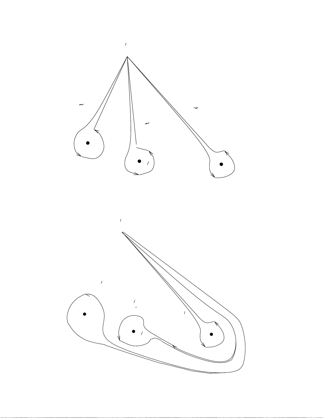
On the Logarithmic Asymptotics of the Sixth P ainlev ´ e Equation (Summer 2007) Da vide Guzzetti Abstract W e compute t h e monod rom y group asso ciated to the solutions of the sixth Painlev ´ e equation with a logarithmic asymptotic b ehavior at a critic al p oin t and we c haracterize the asymptotic b eha vior in terms of the mono dromy itself. 1 In tro duction This paper appea red as a prepr int in August 200 7. It is published in J. Ph ys. A: Math. Theor. 41 , (2008), 20520 1 -2052 47. It was on the archiv e in January 200 8 (a rXiv:0801 .1157). This version do e s not diﬀer from the published one, except for tw o facts: 1)the additio n of subsection 8.2, which prov es that tr( M 0 M x ) = − 2 fo r so lutions y ( x ) ∼ a (ln x ) n , n = 1 , 2, x → 0. 2) The explicit parametrization of the critical b ehavior of the general log-solutions in terms of mono dro m y data, in the last part of Prop ositio n 2. W e c o nsider the sixth Painlev ´ e equation: d 2 y dx 2 = 1 2  1 y + 1 y − 1 + 1 y − x   dy dx  2 −  1 x + 1 x − 1 + 1 y − x  dy dx + y ( y − 1)( y − x ) x 2 ( x − 1) 2  α + β x y 2 + γ x − 1 ( y − 1) 2 + δ x ( x − 1 ) ( y − x ) 2  , (PVI) . The generic solution has essential s ingularities and/or br anch p oints in 0,1, ∞ . It’s behavior at these po in ts is called critic al . Other singularities which ma y app ear are po les and dep end on the initial conditio ns . A solution of (PVI) can be analytically contin ued to a meromor phic function on the universal cov ering o f P 1 \{ 0 , 1 , ∞} . F or generic v alues of the integration constants and of the parameters α , β , γ , δ , it c annot be expressed v ia elementary or cla ssical transcendental functions. F or this reas on, it is calle d a Painlev´ e tr ansc endent . Solving (PVI) means: i) Determine the critical behavior o f the trans cenden ts a t the critic al p oints x = 0 , 1 , ∞ . Such a behavior must depe nd on tw o int egr ation constants. ii) Solv e the c onne ction pr oblem , namely: ﬁnd the relation b etw een couples of integration cons tant s at x = 0 , 1 , ∞ . In this pa p er we compute the mono dro m y g roup asso ciated to the so lutio ns of the sixth Painlev ´ e equation with a logarithmic a symptotic b ehavior, and we para metr ize the as ymptotic b ehavior in terms of the mono dromy itself. 1.1 Associated F uc hsian System (PVI) is the isomono dro my deformation equation of a F uchsian sys tem o f diﬀer e n tial equations [19]: d Ψ dλ = A ( x, λ ) Ψ , A ( x, λ ) :=  A 0 ( x ) λ + A x ( x ) λ − x + A 1 ( x ) λ − 1  , λ ∈ C . (1) The 2 × 2 matrices A i ( x ) depend on x in such a wa y that there exists a fundamental matrix solution Ψ( λ, x ) such that its mono dromy does no t c hange for small defor mations of x . They also dep end o n the parameters α, β , γ , δ of (PVI) through more elementary parameter s θ 0 , θ x , θ 1 , θ ∞ , acco rding to the following r e lations: − A ∞ := A 0 + A 1 + A x = − θ ∞ 2 σ 3 , θ ∞ 6 = 0 . Eigenv alues ( A i ) = ± 1 2 θ i , i = 0 , 1 , x ; (2) 1 α = 1 2 ( θ ∞ − 1) 2 , − β = 1 2 θ 2 0 , γ = 1 2 θ 2 1 ,  1 2 − δ  = 1 2 θ 2 x (3) Here σ 3 :=  1 0 0 − 1  is the Pauli matrix . The condition θ ∞ 6 = 0 is not r estrictive, b ecause θ ∞ = 0 is equiv alent to θ ∞ = 2 . The equatio ns of mono dromy pr e serving defor mation (Schlesinger equations), can b e written in Hamiltonian for m and reduce to (P VI), b eing the tra nscendent y ( x ) the solution λ of A ( x, λ ) 1 , 2 = 0. Namely: y ( x ) = x ( A 0 ) 12 x [( A 0 ) 12 + ( A 1 ) 12 ] − ( A 1 ) 12 , (4) The matrices A i ( x ), i = 0 , x, 1, dep end on y ( x ), dy ( x ) dx and R y ( x ) throug h rational functions, which are given in [1 9] a nd in subsection 8.3. This pap er is devoted to the computation of the mono dro m y gro up of (1 ) asso ciated to the solutions with a logar ithmic critical b ehavior. This is par t of a our pro ject to c la ssify the cr itical behaviors in ter ms of the mono dromy data o f the system (1). This pro ject has b een car ried on through our pap ers [12] [13] [15]. 1.2 Back ground In [15] we developed a matching te chnique . It enabled us to compute the ﬁrst lea ding terms of the critical b ehavior of a tra nscendent y ( x ) in a constructive wa y . Originally , such an appr oach w as suggested by Its a nd Nov okshenov in [16], for the s e cond and third Painlev´ e equations. The metho d of Jim b o [18] ca n b e regar ded as a matching pro cedure. This approach w as further develope d and used by K apaev, Kitaev, Andreev, and V artanian (see fo r example the case of the ﬁfth Painlev´ e equation, in [2]). Our appr o ach of [15] is new, becaus e we intro duced non- fuchsian systems (sy stems with irreg ular singularities) asso cia ted to (P VI). This allo wed us to o btained new asymptotic behaviors. Denote by M 0 , M x , M 1 a mono dromy representation of (1). The critical b ehaviors asso cia ted to mono dr omy matrices satisfying the rela tion tr( M i M j ) 6 = ± 2, i 6 = j ∈ { 0 , x, 1 } , is known from the work [18]. The matc hing pro cedure was dev elop ed in [15], as a genera l metho d to study the c ases tr( M i M j ) = ± 2 and the non generic cases of α, β , γ , δ . The v alues o f the traces tr( M 0 M x ), tr ( M 1 M x ), tr ( M 0 M 1 ) character iz e the critical b ehaviors at x = 0 , 1 , ∞ re s pectively . F or example, in the g eneric case studied in [18] we ﬁnd the following behaviors at the critical p oints [18][10 ][12][13][14][3][26]: y ( x ) =          ax 1 − σ (1 + O ( | x | ǫ )) , x → 0 , y ( x ) = 1 − a (1) (1 − x ) 1 − σ (1) (1 + O ( | 1 − x | ǫ )) , x → 1 , y ( x ) = a ( ∞ ) x σ ( ∞ ) (1 + O ( | x | − ǫ )) , x → ∞ , where ǫ is a small pos itiv e num b er, a , σ , a (1) , σ (1) , a ( ∞ ) , σ ( ∞ ) are complex num b ers such that a , a ( i ) 6 = 0 and 0 < ℜ σ < 1, 0 < ℜ σ (1) < 1 , 0 < ℜ σ ( ∞ ) < 1. The connection problem among the thre e sets o f para meters ( a, σ ), ( a (1) , σ (1) ), ( a ( ∞ ) σ ( ∞ ) ) was ﬁrst solved in [18] and its s olution implies that: 2 cos( πσ ) = tr( M 0 M x ) , 2 cos( π σ (1) ) = tr( M 1 M x ) , 2 cos( π σ ( ∞ ) ) = tr( M 0 M 1 ); while a , a (1) , a ( ∞ ) are rational functions of the tr( M i M j )’s ( i 6 = j = 0 , x, 1 ) and depend o n the θ ν ’s ( ν = 0 , x, 1 , ∞ ) through trigonometric functions and Γ- functions rationally co m bined. In this sense, the three traces determine the critical b ehavior a t the three critical points. 1.3 Critical Beha viors W e summarize the results obtained b y the matc hing pr o cedure in [1 5]. W e consider only the p oint x = 0, beca use the critical b ehaviors at x = 1 , ∞ can b e obtained by the action o f Backlund transformatio ns o f (P VI) ( se e subsectio n 8.4). Let σ b e a complex nu mber deﬁned by: tr( M 0 M x ) = 2 cos( π σ ) , 0 ≤ ℜ σ ≤ 1 . 2 The matching pro ce dur e yields the follo wing b ehaviors for x → 0: y ( x ) ∼ a x 1 − σ , if ℜ σ > 0; (5) y ( x ) ∼ x  iA sin  iσ ln x + φ  + θ 2 0 − θ 2 x + σ 2 2 σ 2  , if ℜ σ = 0 , σ 6 = 0 . In the ab ov e fo r mu lae, σ is one of the integration constants, while a , or φ , is the other. A is: A := " θ 2 0 σ 2 −  θ 2 0 − θ 2 x + σ 2 2 σ 2  2 # 1 2 . F or sp ecial v alues of σ 6 = 0, the ﬁrst leading term ab ov e is zer o and we need to consider the nex t leading terms: y ( x ) ∼ θ 0 θ 0 + θ x x ∓ r θ 0 + θ x x 1+ σ , σ = ± ( θ 0 + θ x ) 6 = 0 , y ( x ) ∼ θ 0 θ 0 − θ x x ∓ r θ 0 − θ x x 1+ σ , σ = ± ( θ 0 − θ x ) 6 = 0 . When σ = 0: y ( x ) ∼ x ( θ 2 x − θ 2 0 4  ln x + 4 r + 2 θ 0 θ 2 0 − θ 2 x  2 + θ 2 0 θ 2 0 − θ 2 x ) , if θ 2 0 6 = θ 2 x , (6) y ( x ) ∼ x ( r ± θ 0 ln x ) , if θ 2 0 = θ 2 x . (7) Here r is an in tegra tion co nstant. In [15] we also computed all the solutions with T aylor expansions at a critical po in t. T aylor solutions are s tudied also in [20], by the is omono dromy deformatio n metho d; and in [4] [5] [6] [7] by a p ow er geo metry technique. In [4] [5] [6] [7 ] [8], A.D.Bruno a nd I.V.Gor yuchkina constructed the asymptotic expansions, including loga r ithmic ones, b y a pow er geometry technique [9]. All the asymptotic expansions obta ined by this technique a re s ummarized in [8], and inc lude – to use the terminolog y of [8 ] – power-logarithmic expa ns ions a nd logarithmic complicated expansio ns. The log arithmic asy mptotics for r eal s olutions of (PVI) is studied in [2 5]. Our approach, b eing bas e d on the metho d o f is omono dromy deformatio ns, allows to so lve the connection pro blem, while the results [4]– [8] and [25] are lo cal. The mono dr omy data for the so lutio n (5) a r e computed in [18][10][12][13][14][3]. The mo no dr omy data for the T aylor expansions are computed in [15] and [20]. The mono dromy asso cia ted to the logar ithmic b ehaviors ar e no t known. Their c o mputation is the main result of the present paper. W e are going to s how that logarithmic critical behaviors at x = 0 are asso ciated to tr( M 0 M x ) = ± 2, at x = 1 to tr( M 1 M x ) = ± 2, and at x = ∞ to tr( M 0 M 1 ) = ± 2. 1.4 Results of this Paper In this pap er: 1) In Section 3 we justify the pr o ject o f classifying the transc e nden ts in terms o f mono dromy data o f (1). W e establis h the necessa ry and suﬃcient conditions such that ther e exist a one to one corres p ondence betw een a s et o f mono dromy data of sys tem (1) and a trans cendent of (PVI). The result is Prop ositio n 1. The deﬁnition of mono dr omy data itself is given in Section 3 . 2) W e compute the mo no dr omy data asso cia ted to the loga rithmic solutions (6) in the generic case θ 0 , θ x , θ 1 , θ ∞ 6∈ Z . The res ult is Prop osition 2, Section 5 . In par ticular, tr( M 0 M x ) = 2. 3) In Pro po sition 3 of Section 6, we compute the mo no dromy gro up asso ciated to the solution (7). In particular , tr ( M 0 M x ) = 2. The pa rameter r will b e co mputed as a function of the θ ν ’s, ν = 0 , x, 1 , ∞ and of tr( M 0 M 1 ). 4) W e consider a non gener ic ca se of (6 ), which o ccur s when: θ x = θ 1 = 0 , θ ∞ = 1 , θ 0 = 2 p 6 = 0 , p ∈ Z . (8) 3 Therefore: y ( x ) ∼ x " 1 − p 2  ln x + r + p p 2  2 # , x → 0 . (9) The mono dr omy of the asso c ia ted system (1) is computed in Pr o po sition 4, Sec tio n 7. It is imp ortant to observe tha t the mono dromy is indep endent of r . This means that the parameter r cannot b e determined in terms o f the mono dromy data. Therefor e, (9) is a one p ar ameter class of solutions ( parameter r ) asso ciate d to the same mono dr omy data . W e prov e in Pr o po sition 4 tha t the solution (9) is asso cia ted to: tr( M 0 M x ) = 2 , tr( M 0 M 1 ) = 2 , tr( M 1 M x ) = − 2 . This sp ecial v alues of the tra ces imply that the b ehavior at x = ∞ a nd x = 1 is also loga rithmic. tr( M 0 M x ) = 2 is asso ciated to the lo garithmic b ehavior of t yp e ln 2 x a t x = 0. tr( M 0 M 1 ) = 2 is asso ciated to the log a rithmic b ehavior of t yp e ln 2 (1 /x ) at x = ∞ . tr ( M 1 M x ) = − 2 is asso cia ted to the loga rithmic b ehavior o f type 1 / ln 2 (1 − x ) at x = 1. Actually a solution (9) has the following behaviors at the three critical p oints: y ( x ) ∼            x  1 − p 2 (ln x + ρ 0 ) 2  , x → 0 , 1 − p 2  ln 1 x + ρ ∞  2 , x → ∞ , 1 − 1 p 2 (ln(1 − x )+ ρ 1 ) 2 , x → 1 . (10) where: ρ 0 = ( r + p ) p 2 , ρ ∞ = π (4 ln 2 − 1 + ρ 0 ) π − i (4 ln 2 − 1 + ρ 0 ) − 2 ln 2 + 1 , ρ 1 = π 2 4 ln 2 − 1 + ρ 0 − ln 2 + 1 . The b ehavior at x = 1 diﬀers from those at x = 0 , ∞ for the inv erse of ln(1 − x ) appea rs. This is actually due to the fact that tr( M 1 M x ) = − 2. W e w ill prov e the ab ov e behaviors in section 8.5, and in the second pap er b y a diﬀerent method. In general, the logarithmic behaviors of “type (6)” at the critical p oints are as follows:                y ( x ) ∼ x  θ 2 x − θ 2 0 4 h ln x + 4 r + 2 θ 0 θ 2 0 − θ 2 x i 2 + θ 2 0 θ 2 0 − θ 2 x  , x → 0 . y ( x ) ∼ θ 2 0 θ 2 0 − θ 2 1 + θ 2 1 − θ 2 0 4 h ln 1 x + 4 r + 2 θ 0 θ 2 0 − θ 2 1 i 2 , x → ∞ . y ( x ) ∼ 1 − (1 − x )  θ 2 1 θ 2 1 − θ 2 x + θ 2 x − θ 2 1 4 h ln(1 − x ) + 4 r + 2 θ 1 θ 2 1 − θ 2 x i 2  , x → 1 . (11)            y ( x ) = 4 [ θ 2 1 − ( θ ∞ − 1) 2 ] ln 2 x h 1 + 8 r + 4 θ ∞ − 4 θ 2 1 − ( θ ∞ − 1) 2 1 ln x + O  1 ln 2 x  i , x → 0 . y ( x ) = 4 x [( θ ∞ − 1) 2 − θ 2 x ] ln 2 x h 1 − 8 r + 4( θ ∞ − 1) θ 2 x − ( θ ∞ − 1) 2 1 ln x + O  1 ln 2 x  i , x → ∞ . y ( x ) = 1 + 4 ( θ 2 1 − θ 2 0 ) ln 2 ( x − 1) h 1 − 8 r + 4 θ 0 θ 2 0 − θ 2 1 1 ln( x − 1) + O  1 ln 2 ( x − 1) i , x → 1 . (12) W e stres s that a solutio n with a log -b ehavior at x = 0 (for example) do es not nec essarily hav e a log-b ehavior at x = 1 or x = ∞ . The case (9) is specia l, in that the log -b ehavior appear s at the three critical p oints. In general, the log-b ehaviors of “type (7)” ar e :          y ( x ) ∼ x ( r ± θ 0 ln x ) , x → 0 , θ 2 0 = θ 2 x . y ( x ) ∼ r ± θ 0 ln x, x → ∞ , θ 2 0 = θ 2 1 . y ( x ) ∼ 1 − (1 − x )  r ± θ 1 ln(1 − x )  , x → 1 , θ 2 1 = θ 2 x . (13) 4            y ( x ) = 1 r ± ( θ ∞ − 1) ln x  1 + O  1 ln x  , x → 0 , ( θ ∞ − 1) 2 = θ 2 1 . y ( x ) = ± x ( θ ∞ − 1) ln x h 1 ∓ r ( θ ∞ − 1) ln x + O  1 ln 2 x  i , x → ∞ , ( θ ∞ − 1) 2 = θ 2 x . y ( x ) = 1 ± 1 θ 0 ln( x − 1) h 1 ∓ r θ 0 ln( x − 1) + O  1 ln 2 ( x − 1) i , x → 1 , ( θ ∞ − 1) 2 = θ 2 0 . (14) The above are prov e d in Section 8 , making use o f the B a cklund transformations of (PVI). The behaviors in (11), (13) a r e asso cia ted to tr( M 0 M x ) = 2 when x → 0; to tr( M 0 M 1 ) = 2 when x → ∞ ; to tr( M 1 M x ) = 2 when x → 1. This fact is proved in Section 8.4. The b ehaviors in (12), (14) are asso ciated to tr( M 0 M x ) = − 2 when x → 0; to tr( M 0 M 1 ) = − 2 when x → ∞ ; to tr( M 1 M x ) = − 2 when x → 1. This fa c t is prov ed in section 8.2. Ac knowledgment s: The pap er was written a t RIMS, Kyoto University , supp orted by the Kyoto Mathematics COE. 2 Matc hing Pro cedure This se ction is a review of the matching pro cedure of [15]. W e explain how the asymptotic b ehavior of a transcendent is der ived, and how the ass o ciated mo no dromy is computed. 2.1 Leading T erms of y ( x ) W e consider x → 0. W e divide the λ -plane into tw o domains. The “ outside” domain is deﬁned for λ suﬃciently big: | λ | ≥ | x | δ OU T , δ OU T > 0 . (15) Therefore, (1) can b e written as: d Ψ dλ = " A 0 + A x λ + A x λ ∞ X n =1  x λ  n + A 1 λ − 1 # Ψ . (16) The “inside” domain is deﬁned for λ compara ble with x , namely: | λ | ≤ | x | δ I N , δ I N > 0 . (17) Therefore, λ → 0 as x → 0, and we rewr ite (1) as: d Ψ dλ = " A 0 λ + A x λ − x − A 1 ∞ X n =0 λ n # Ψ . (18) If the b ehavior of A 0 ( x ), A 1 ( x ) and A x ( x ) is suﬃciently go o d, we expect that the higher or der terms in the series of (16 ) a nd (1 8) are s mall corrections which can b e neglected when x → 0. If this is the case, (16) and (18) reduce resp ectively to : d Ψ OU T dλ = " A 0 + A x λ + A x λ N OU T X n =1  x λ  n + A 1 λ − 1 # Ψ OU T , (19) d Ψ I N dλ = " A 0 λ + A x λ − x − A 1 N I N X n =0 λ n # Ψ I N , (20) where N I N , N OU T are suitable int eger s. The simplest r e ductio n is to F uchsian sys tems: d Ψ OU T dλ =  A 0 + A x λ + A 1 λ − 1  Ψ OU T , (21) d Ψ I N dλ =  A 0 λ + A x λ − x  Ψ I N . (22) 5 In [15] w e co nsidered reduced non-fuc hsian sys tems for the ﬁrst time in the litera tur e, where the fuc hsian reduction has b een priv ileged. W e show ed that in some relev ant ca ses it cannot b e used, being the non-fuchsian reductio n necessary . Generally s pea king, we ca n par ameterize the elements of A 0 + A x and A 1 of (21 ) in terms of θ 1 , the eigenv a lue s of A 0 + A x and the eigenv alues θ ∞ of A 0 + A x + A 1 . W e also need an a dditional unknown function of x . In the same wa y , we ca n explicitly para meterize the elements of A 0 and A x in (22) in terms of θ 0 , θ x , the eigenv alues of A 0 + A x and another a dditional unknown function of x . Cases when the reductions (19) and (20 ) are non- fuc hsian deserve particula r care, as it has b e en done in [15]. O ur purp os e is to ﬁnd the leading terms of the unknown functions when x → 0, in order to determine the critical b ehavior o f A 0 ( x ), A 1 ( x ), A x ( x ) and of (4). The leading term can be o btained as a result of t wo facts: i) Systems (19) and (20) a re is omono dromic. This imp oses constraints on the form o f the unkno wn functions. Typically , one of them m ust b e constant. ii) Two fundamen tal matrix solutions Ψ OU T ( λ, x ), Ψ I N ( λ, x ) must match in the region of overlap, provided this is not empty: Ψ OU T ( λ, x ) ∼ Ψ I N ( λ, x ) , | x | δ OU T ≤ | λ | ≤ | x | δ I N , x → 0 (23) This relation is to b e in tended in the se ns e that the leading terms o f the lo cal behavior o f Ψ OU T and Ψ I N for x → 0 must be equal. This determines a simple relatio n betw een the t wo functions of x app earing in A 0 , A x , A 1 , A 0 + A x . (23 ) also implies that δ I N ≤ δ OU T . Practica lly , to fulﬁll p oint ii), w e matc h a fundamen tal solution o f (1 9) for λ → 0, with a fundamen tal solution of the s y stem obtaine d from (20) b y the change of v ariables µ := λ/x , namely with a solution of: d Ψ I N dµ = " A 0 µ + A x µ − 1 − xA 1 N I N X n =0 x n µ n # Ψ I N , µ := λ x . (24) T o summarize, matching tw o fundamen tal so lutions of the reduced isomono dr omic systems (19) and (20), we obtain the le a ding term(s), for x → 0, of the entries of the matr ices of the or iginal system (1). The pro cedure is algor ithmic, the only assumption b eing (23). This metho d is sometimes called c o alesc enc e of singularities , b eca use the sing ularity λ = 0 and λ = x coalesc e to pro duce sys tem (19), while the sing ularity µ = 1 x and µ = ∞ co a lesce to pro duce system (24). Coalescence of singularities was ﬁrst used b y M. Jim b o in [18] to co mpute the mono dromy matrices of (1 ) for the class of solutions of (P VI) with le ading ter m y ( x ) ∼ a x 1 − σ , 0 < ℜ σ < 1. 2.2 Computation of the Mono drom y Data In the “ λ -plane” C \{ 0 , x, 1 } we ﬁx a base p oint λ 0 and thre e lo ops , whic h are num b ere d in or der 1, 2, 3 accor ding to a co un ter-c lo c kwise or der referred to λ 0 . W e choos e 0 , x, 1 to b e the or der 1 , 2 , 3. W e denote the lo ops by γ 0 , γ x , γ 1 . See ﬁgur e 1. The mono dromy matr ices o f a fundamen tal solution Ψ( λ ) w.r .t. this base of lo ops are deno ted M 0 , M x , M 1 . The lo o p at inﬁnit y will b e γ ∞ = γ 0 γ x γ 1 , so M ∞ = M 1 M x M 0 . As a cons e quence, the following relation holds: cos( π θ 0 )tr( M 1 M x ) + cos( π θ 1 )tr( M 0 M x ) + cos( π θ x )tr( M 1 M 0 ) = 2 cos( π θ ∞ ) + 4 cos( π θ 1 ) cos( π θ 0 ) cos( π θ x ) . The mono dromy matrices ar e determined b y tr( M ν ), tr( M ν M µ ) , ν, µ = 0 , x, 1 , ∞ [3]. As a conseq uence of isomono dr omicity , there exists a fundamen tal so lution Ψ OU T of (19 ) such that M OU T 1 = M 1 , M OU T ∞ = M ∞ , where M OU T 1 and M OU T ∞ are the mono dromy matrices of Ψ OU T at λ = 1 , ∞ . Moreov er, M OU T 0 = M x M 0 . Ther e also ex is ts a fundamen tal solution Ψ I N of (20) such that: M I N 0 = M 0 , M I N x = M x , 6 0 x 1 γ γ γ 0 x 1 1 2 3 order 1, 2, 3. λ 0 Figure 1: The ordered basis of loo ps where M I N 0 and M I N x are the mono dromy matrices of Ψ I N at λ = 0 , x . The method of coalesce nc e of singularities is useful when the mono dr omy o f the reduced sys tems (19), (20) can b e ex plicitly computed. This is the case when the reduction is fuch sia n (namely (21), (22)), bec a use fuc hsia n sy stems with three singular p oints are e quiv alent to a Gauss h yp er- geometric eq uation (see Appendix 1). F or the non-fuchsian reduction, in g eneral we can compute the mono dromy when (19), (20 ) are solv able in terms of spec ial or elemen tary functions. In order for this pro c edure to work, not only Ψ OU T and Ψ I N m ust match with eac h o ther, as in subsection 2.1, but also Ψ OU T m ust match with a fundamental matrix solution Ψ of (1) in a domain of the λ plane, and Ψ I N m ust match with the same Ψ in another domain of the λ plane. The standard c hoice of Ψ is as follows: Ψ( λ ) =                     I + O  1 λ  λ − θ ∞ 2 σ 3 λ R ∞ , λ → ∞ ; ψ 0 ( x )  I + O ( λ )  λ θ 0 2 σ 3 λ R 0 C 0 , λ → 0; ψ x ( x )  I + O ( λ − x )  ( λ − x ) θ x 2 σ 3 ( λ − x ) R x C x , λ → x ; ψ 1 ( x )  I + O ( λ − 1)  ( λ − 1) θ 1 2 σ 3 ( λ − 1) R 1 C 1 , λ → 1; (25) Here ψ 0 ( x ), ψ x ( x ), ψ 1 ( x ) ar e the diagonaliz ing matr ices of A 0 ( x ), A 1 ( x ), A x ( x ) res pectively . They are deﬁned by m ultiplication to the right b y arbitrary diago nal matrices, p oss ibly dep ending on x . C ν , ν = ∞ , 0 , x, 1, are inv ertible c onne ction matric es , indep endent of x [1 9]. Each R ν , ν = ∞ , 0 , x, 1, is also independent of x , and: R ν = 0 if θ ν 6∈ Z , R ν =         0 ∗ 0 0  , if θ ν > 0 integer  0 0 ∗ 0  , if θ ν < 0 integer 7 If θ i = 0, i = 0 , x, 1 , then R i is to be considered the Jor dan form  0 1 0 0  of A i . Note that for the lo op λ 7→ λe 2 π i , | λ | > max { 1 , | x |} , w e immediately compute the mono dr omy at inﬁnit y: M ∞ = ex p { − iπ θ ∞ } ex p { 2 π iR ∞ } . Let Ψ OU T and Ψ I N be the solutions of (19) and (20) matching as in (23 ). W e explain how they are matched with (2 5). (*) Matc hing Ψ ↔ Ψ OU T : λ = ∞ is a fuc hsian singula r it y of (19), with residue − A ∞ /λ . Ther efore, we can alwa ys ﬁnd a fundamen tal ma tr ix solution with behavior: Ψ M atch OU T =  I + O  1 λ  λ − θ ∞ 2 σ 3 λ R ∞ , λ → ∞ . This solution matches with Ψ. Also λ = 1 is a fuchsian sing ularity of (19). Therefore , we hav e: Ψ M atch OU T = ψ OU T 1 ( x )  I + O ( λ − 1)  ( λ − 1) θ 1 2 σ 3 ( λ − 1) R 1 C OU T 1 , λ → 1; Here C OU T 1 is a suita ble c onnection ma tr ix. ψ OU T 1 ( x ) is the ma trix that diag onalizes the leading terms of A 1 ( x ). Ther efore, ψ 1 ( x ) ∼ ψ OU T 1 ( x ) for x → 0. As a c o nsequence of isomono dr omicity , R 1 is the same of Ψ. As a consequence of the match ing Ψ ↔ Ψ M atch OU T , the mono dromy of Ψ at λ = 1 is: M 1 = C 1 − 1 exp { iπ θ 1 σ 3 } exp { 2 π iR 1 } C 1 , with C 1 ≡ C OU T 1 . W e ﬁnally need a n inv ertible connection ma trix C OU T to co nnect Ψ M atch OU T with the so lutio n Ψ OU T app earing in (23). Namely , Ψ M atch OU T = Ψ OU T C OU T . (*) Matc hing Ψ ↔ Ψ I N : As a cons equence o f the matching Ψ ↔ Ψ M atch OU T , we hav e to choo se the IN-so lution which matches with Ψ M atch OU T . This is Ψ M atch I N := Ψ I N C OU T . Now, λ = 0 , x are fuc hsian singularities of (20). Therefor e : Ψ M atch I N =    ψ I N 0 ( x )  I + O ( λ )  λ θ 0 2 σ 3 λ R 0 C I N 0 , λ → 0; ψ I N x ( x )  I + O ( λ − x )  ( λ − x ) θ x 2 σ 3 ( λ − x ) R x C I N x , λ → x ; The a b ove hold for ﬁxed s mall x 6 = 0. Here C I N 0 and C I N x are suitable connection matrices. ψ I N 0 ( x ) and ψ x ( x ) I N are diagona lizing matrices of the leading terms of A 0 ( x ) and A x ( x ). F or x → 0 they match with ψ 0 ( x ) and ψ x ( x ) of Ψ in (28). On the o ther hand, as a conse quence of isomo no dr omicity , the matric e s R 0 and R x are the same of Ψ. The ab ov e Ψ M atch I N has the sa me behavior of Ψ at λ → 0 and λ → x ; moreover, it is a n approximation of Ψ for x s mall. The matr ices C I N 0 , C I N x are independent o f x . So , the matching Ψ ↔ Ψ I N is realized and the connection matrices C 0 and C x coincide with C I N 0 , C I N x resp ectively . As a result, we obtain the mono dro my matrices fo r Ψ : M 0 = C 0 − 1 exp { iπ θ 0 σ 3 } exp { 2 π i R 0 } C 0 , C 0 ≡ C I N 0 , M x = C x − 1 exp { iπ θ x σ 3 } exp { 2 π i R x } C x , C x ≡ C I N x . Our re ductio n is us eful if the connectio n matrices C OU T 1 , C I N 0 , C I N x can b e computed explicitly . This is p ossible for the fuchsian reduced systems (21), (22). F or non-fuch sia n reduced systems, we discussed the computability in [15]. 8 3 Classiﬁcation in T erms of Mono drom y Data Two conjuga ted systems: d Ψ dλ = A ( x, λ ) Ψ , d ˜ Ψ dλ = ˜ A ( x, λ ) ˜ Ψ , ˜ Ψ = W Ψ , det( W ) 6 = 0 , ˜ A = W AW − 1 , admit fundament al matrix solutions with the sa me mono dro m y matrices (w.r.t. the s ame basis of lo ops). The matrix ˜ A ( x, λ ) deﬁnes the same so lutio n of (PVI) asso ciated to A ( x, λ ) o nly if the following co ndition holds: ˜ A 0 + ˜ A 1 + ˜ A x = − θ ∞ 2 σ 3 , where ˜ A i = W A i W − 1 , i = 0 , x, 1 . Namely , W σ 3 W − 1 = σ 3 . This o ccurs if and o nly if W is diago nal . The transformation of A ( x, λ ) is therefore: W A ( x, λ ) W − 1 =  A 11 ( x, λ ) w 2 w 1 A 12 ( x, λ ) w 1 w 2 A 21 ( x, λ ) A 22 ( x, λ )  , where W =  w 1 0 0 w 2  . W e conclude tha t the equation A 12 ( x, λ ) = 0 is the same and then: Two c onjugate fuchsian systems, satisfying (2) (3), deﬁne the same solution of PVI if and only if the c onjugation is diag onal. Note that θ ∞ 6 = 0 is a necess ary condition, other wise any W would be acc e ptable and then A 12 ( x, λ ) = 0 w ould not deﬁne y ( x ) uniquely . The problem of ﬁnding a (branch of a) tra nscendent asso cia ted to a mono dromy repres ent ation is the pr oblem o f ﬁnding a fuc hsia n system (1) having the g iven mono dro m y . This pr oblem is called Riema nn- Hilb ert pr oblem , or 21 th Hilb ert pr oblem . F or a g iven P VI there is a one-to-o ne corres p ondence b et ween a monodr omy representation a nd a br anch of a transcendent if and only if the Riemann-Hilb ert problem has a unique solution A ( x, λ ), deﬁned up to diagona l conjugation. • Rie mann-Hilb e rt problem (R.H. ) : ﬁnd the co eﬃcie n ts A i ( x ), i = 0 , x, 1 from the following mono dr omy data : a) A ﬁxe d or der o f the p oles 0 , x, 1. Namely , we choo se a base of loo ps. Her e w e choose the order (1,2,3)=(0, x ,1). See ﬁgure 1. b) The exp o nent s θ 0 , θ x , θ 1 , θ ∞ , with θ ∞ 6 = 0. The res tr iction θ ∞ 6 = 0 is just tec hnical, due to the present deﬁnition of θ ∞ , and is not a limitation, bec ause b y deﬁnition θ ∞ = 0 is equiv alent to θ ∞ = 2. c) Matrices R 0 , R x , R 1 , R ∞ , such that: R ν = 0 if θ ν 6∈ Z , R ν =         0 ∗ 0 0  , if θ ν > 0 integer  0 0 ∗ 0  , if θ ν < 0 integer R j =  0 1 0 0  , if θ j = 0 , j = 0 , x, 1 . c) three mono dromy matrices M 0 , M x , M 1 relative to the lo ops, similar to the matrices exp { i π θ i σ 3 } exp { 2 π iR i } , i = 0 , x, 1, satisfying (for the chosen o rder of lo o ps γ 0 γ x γ 1 = γ ∞ ): M 1 M x M 0 = e − iπθ ∞ σ 3 e 2 π iR ∞ Solving the Riemann- Hilber t pro blem mea ns that we have to ﬁnd in vertible c onne ction matric es , C ν , ν = ∞ , 0 , x, 1, such tha t. C − 1 j e iπθ j σ 3 e 2 π iR j C j = M j , j = 0 , x, 1 ; (26) C − 1 ∞ e − iπθ ∞ σ 3 e 2 π iR ∞ C ∞ = e − iπθ ∞ σ 3 e 2 π iR ∞ . (27) 9 and a matrix v alued mer o morphic function Ψ( x, λ ) s uch that: Ψ( x, λ ) =                     I + O  1 λ  λ − θ ∞ 2 σ 3 λ R ∞ C ∞ , λ → ∞ ; ψ 0 ( x )  I + O ( λ )  λ θ 0 2 σ 3 λ R 0 C 0 , λ → 0; ψ x ( x )  I + O ( λ − x )  ( λ − x ) θ x 2 σ 3 ( λ − x ) R x C x , λ → x ; ψ 1 ( x )  I + O ( λ − 1)  ( λ − 1) θ 1 2 σ 3 ( λ − 1) R 1 C 1 , λ → 1; (28) Here ψ 0 , ψ x , ψ 1 are inv ertible matrices dep ending on x . The co e ﬃcie n t of the fuc hsian system ar e then given by A ( x ; λ ) := d Ψ( x, λ ) dλ Ψ( x ; λ ) − 1 . A 2 × 2 R.H. is alw ays solv able at a ﬁxed x [1]. As a function of x , the so lution A ( x ; λ ) extends to a mer omorphic function on the univ ers al cov ering of ¯ C \{ 0 , 1 , ∞} . Now we prov e the following fact: The R.H. admits diagonal ly c onjugate d s olut ions (fuchsian systems), exc ept when at le ast one θ ν ∈ Z \{ 0 } and simultane ou s ly R ν = 0 . This can be equiv alently sta ted in the form of the follo wing: Prop ositio n 1 Ther e is a one to one c orr esp ondenc e b etwe en t he mono dromy data θ 0 , θ x , θ 1 , R 0 , R x , R 1 , θ ∞ 6 = 0 , R ∞ , M 0 , M x , M 1 (deﬁne d up to c onjugation), satisfying a), b), c) ab ove, and a (br anch of a) tr ansc endent y ( x ) , exc ept when at le ast one θ ν ∈ Z \{ 0 } and simultane ou s ly R ν = 0 . T o s ay in other words, the one to o ne corres po ndence is realized if and o nly if one of the following conditions is satisﬁed: (1) θ ν 6∈ Z , for every ν = 0 , x, 1 , ∞ ; (2) if some θ ν ∈ Z a nd R ν 6 = 0 , θ ν 6 = 0 (3) if some θ j = 0 ( j = 0 , x, 1) and sim ultaneously θ ∞ 6∈ Z , o r θ ∞ ∈ Z and R ∞ 6 = 0 . Note that for θ j = 0, M j can be put in Jorda n form  1 2 π i 0 1  . Therefore Prop osition 1 says that: Ther e is one to one c orr esp ondenc e exc ept when one of t he matric es M i ( i = 0 , x, 1 ), or M ∞ = M 1 M x M 0 , is e qual to ± I . Pr o of: The pro of is base d on the o bserv a tion that a triple of mono dro m y matrice s M 0 , M x , M 1 may be r e alized by tw o fuchsian systems which are not c o njugated. The crucial p oint is that the solutions of (26 ), (27 ) are not unique. Two sets o f particula r solutions C ν and ˜ C ν ( ν = 0 , x, 1 , ∞ ) give to fuchsian systems: d Ψ( x, λ ) dλ Ψ( x, λ ) − 1 = A ( x, λ ) , d ˜ Ψ( x, λ ) dλ ˜ Ψ( x, λ ) − 1 = ˜ A ( x, λ ) . These may b e not diago nally conjugated. If this happ ens, there is no one- to-one corresp ondence betw een a set o f mo no dromy data and a solutions of PVI. W e study the struc tur e of the so lutions of (26), (27). E quation (27) ha s the following solutions : i) If θ ∞ 6∈ Z (a nd then R ∞ = 0 ), C ∞ =  p ∞ 0 0 q ∞  , p ∞ , q ∞ ∈ C \{ 0 } ii) If θ ∞ ∈ Z a nd R ∞ 6 = 0, C ∞ =  p ∞ q ∞ 0 p ∞  , if R ∞ =  0 ∗ 0 0  10 C ∞ =  p ∞ 0 q ∞ p ∞  , if R ∞ =  0 0 ∗ 0  . where p ∞ , q ∞ ∈ C , p ∞ 6 = 0 . iii) If θ ∞ ∈ Z and R ∞ = 0, then C ∞ is any inv e r tible matrix. Equation (26), may have diﬀeren t so lutio ns C j and ˜ C j . Therefore C j ˜ C − 1 j is a solution of:  C j ˜ C − 1 j  − 1 e iπθ j σ 3 e 2 π iR j C j ˜ C − 1 j = e iπθ j σ 3 e 2 π iR j . i) If θ j 6∈ Z (and then R j = 0 ), w e hav e: C j ˜ C − 1 j =  a j 0 0 b j  , a j , b j ∈ C \{ 0 } ii) If θ j ∈ Z a nd R j 6 = 0 , w e hav e : C j ˜ C − 1 j =  a j b j 0 a j  , a j , b j ∈ C , a j 6 = 0; if R j =  0 ∗ 0 0  C j ˜ C − 1 j =  a j 0 b j a j  , a j , b j ∈ C , a j 6 = 0 ; if R j =  0 0 ∗ 0  . In particular, for θ j = 0 , R j is the Jordan form  0 1 0 0  . iii) If θ j ∈ Z a nd R j = 0 , then C j ˜ C − 1 j is an y inv ertible matrix  a b c d  . Let C ν and ˜ C ν ( ν = 0 , x, 1 , ∞ ) be tw o sets o f solutions of (26) (27) and let us denote by Ψ and ˜ Ψ the corr esp onding solutions of the R.H. W e observe that: i) for θ j 6∈ Z ( j = 0 , x, 1 ): ( λ − j ) θ j 2 σ 3  a j 0 0 b j  =  a j 0 0 b j  ( λ − j ) θ j 2 σ 3 . ii) F or θ j ∈ Z and R j 6 = 0 : ( λ − j ) θ j 2 σ 3 ( λ − j ) R j  a j b j 0 a j  =  a j I + ( λ − j ) | θ j |  0 b j 0 0  ( λ − j ) θ j 2 σ 3 ( λ − j ) R j , or ( λ − j ) θ j 2 σ 3 ( λ − j ) R j  a j 0 b j a j  =  a j I + ( λ − j ) | θ j |  0 0 b j 0  ( λ − j ) θ j 2 σ 3 ( λ − j ) R j , for R j upper or low e r triangula r r esp ectively . iii) F or θ j ∈ Z a nd R j = 0 : ( λ − j ) θ j 2 σ 3  a b c d  =  a bλ θ j cλ − θ j d  ( λ − j ) θ j 2 σ 3 W e conclude that, for λ → j : Ψ ˜ Ψ − 1 ∼                                   a j 0 0 b j  , if θ j 6∈ Z ;      a j I , if θ j 6 = 0 ,  a j b j 0 a j  , if θ j = 0 , if θ j ∈ Z , R j 6 = 0    Arbitrary in vert. matrix, if θ j = 0 , C ( λ − j ) −| θ j | → ∞ , otherwise , if θ j ∈ Z , R j = 0 11 The matrix C a bove is C =  0 ∗ 0 0  or C =  0 0 ∗ 0  . Let C ∞ and ˜ C ∞ be t wo so lutions of (27). i) If θ ∞ 6∈ Z (a nd then R ∞ = 0 ), w e hav e C ∞ ˜ C − 1 ∞ =  a ∞ 0 0 b ∞  , a ∞ , b ∞ ∈ C \ { 0 } . ii) If θ ∞ ∈ Z a nd R ∞ 6 = 0, we ha ve C ∞ ˜ C − 1 ∞ =  a ∞ b ∞ 0 a ∞  , a ∞ , b ∞ ∈ C , a ∞ 6 = 0 ; if R ∞ =  0 ∗ 0 0  C ∞ ˜ C − 1 ∞ =  a ∞ 0 b ∞ a ∞  , a ∞ , b ∞ ∈ C , a ∞ 6 = 0; if R ∞ =  0 0 ∗ 0  . iii) If θ ∞ ∈ Z and R ∞ = 0, then C ∞ ˜ C − 1 ∞ is any in vertible ma trix. Therefore, for λ → ∞ we hav e: Ψ ˜ Ψ − 1 ∼             a ∞ 0 0 b ∞  if θ ∞ 6∈ Z ;  I + O  1 λ   a ∞ I + b ∞ λ | θ ∞ |  → a ∞ I , if θ ∞ ∈ Z \{ 0 } , R ∞ 6 = 0 C ∞ λ | θ ∞ | → ∞ , if θ ∞ ∈ Z \{ 0 } , R ∞ = 0 The matrix C ∞ ab ov e is C ∞ =  0 ∗ 0 0  or C ∞ =  0 0 ∗ 0  . F rom the above result we co nclude that Ψ ˜ Ψ − 1 is a nalytic o n ¯ C and then it is a constant matrix W , except when at lea st o ne θ ν ∈ Z \ { 0 } and sim ultaneously R ν = 0 . Except for this case, w e have: Ψ = W ˜ Ψ = ⇒ ˜ A ( x, λ ) = W A ( x, λ ) W − 1 . W e observe that: W = lim λ →∞ Ψ ˜ Ψ − 1 (in the cases θ ∞ 6∈ Z , or for θ ∞ ∈ Z ( θ ∞ 6 = 0 ) and R ∞ 6 = 0). Therefore W is diagonal. Prop ositio n 1 is prov ed. ✷ 4 Logarithmic asymptotics (6) and (7) W e cons ider ca ses when (1) can be reduced to the fuchsian systems (21) a nd (22). Let σ b e a complex num be r deﬁned, up to sign, b y: tr ( M 0 M x ) = 2 cos( πσ ) , |ℜ σ | ≤ 1 . In our pap er [15], we co mputed all the asymptotic b ehaviors for 0 ≤ ℜ σ < 1, as they can b e obtained from the ma tc hing pro cedure when (21 ) and (22) are fuchsian. Among them, w e obtained (6) and (7). Note: F or so lutio ns with expansion: y ( x ) = x ( A 1 + B 1 ln x + C 1 ln 2 x + D 1 ln 3 x + ... ) + x 2 ( A 2 + B 2 ln x + ... ) + ..., x → 0 . only the following cas es a re pos sible: y ( x ) =          θ 0 θ 0 ± θ x x + O ( x 2 ) [T aylor expansion] , x  θ 2 0 − B 2 1 θ 2 0 − θ 2 x + B 1 ln x + θ 2 x − θ 2 0 4 ln 2 x  + x 2 ( ... ) + ..., x ( A 1 ± θ 0 ln x ) + x 2 ( ... ) + ..., and θ 0 = ± θ x . (29) A 1 and B 1 are parameter s. W e se e that the higher orders in (6) and (7) are O ( x 2 ln m x ), for some int eger m > 0 . 12 4.1 Review of the Deriv ation of (6) and (7) Let x → 0. The r eduction to the fuc hsian systems (21) is p ossible if in the domain (15) we have: | ( A 0 + A x ) ij | ≫    ( A x ) ij x λ    , namely : | ( A 0 + A x ) ij | ≫   ( A x ) ij x 1 − δ OU T   . (30) Let us denote with ˆ A i the leading term of the matrix A i , i = 0 , x, 1. W e c a n substitute (21) with: d Ψ OU T dλ = " ˆ A 0 + ˆ A x λ + ˆ A 1 λ − 1 # Ψ OU T (31) Lemma 1 If the appr oximation (21) is p ossible, then ˆ A 0 + ˆ A x has eigenvalues ± σ 2 ∈ C indep endent of x , deﬁne d (up to sign and addi tion of an inte ger) by tr ( M x M 0 ) = 2 co s( π σ ) . L et r 1 ∈ C , r 1 6 = 0 . F or θ ∞ 6 = 0 , the le ading terms ar e: ˆ A 1 = σ 2 − θ 2 ∞ − θ 2 1 4 θ ∞ − r 1 [ σ 2 − ( θ 1 − θ ∞ ) 2 ][ σ 2 − ( θ 1 + θ ∞ ) 2 ] 16 θ 2 ∞ 1 r 1 − σ 2 − θ 2 ∞ − θ 2 1 4 θ ∞ ! , (32) and ˆ A 0 + ˆ A x = θ 2 1 − σ 2 − θ 2 ∞ 4 θ ∞ r 1 − [ σ 2 − ( θ 1 − θ ∞ ) 2 ][ σ 2 − ( θ 1 + θ ∞ ) 2 ] 16 θ 2 ∞ 1 r 1 − θ 2 1 − σ 2 − θ 2 ∞ 4 θ ∞ ! . (33) Pr o of: Observ e that tr( ˆ A 0 + ˆ A x ) = tr( A 0 + A x ) = 0, thus, for any x , ˆ A 0 + ˆ A x has eige n v a lues of opp os ite sign, that we denote ± ˜ σ ( x ) / 2. Then, w e r ecall tha t x is a monodr omy prese r ving deformation, therefore the monodr omy matrices o f (3 1) are indep endent of x . At λ = 0 , 1 , ∞ they are: M OU T 0 =  M x M 0 M 0 M x , M OU T 1 = M 1 , M OU T ∞ = M ∞ . Thu s, det( M OU T 0 ) = 1, b ecause det( M x )=det( M 0 ) = 1. Therefor e, there exists a constant matrix D and a complex constant num be r σ suc h that: D − 1 M OU T 0 D =      diag(exp {− iπ σ } , exp { iπ σ } ) ,  ± 1 ∗ 0 ± 1  , or  ± 1 0 ∗ ± 1  , σ ∈ Z W e conclude tha t ˜ σ ( x ) ≡ σ . W e also hav e tr( M OU T 0 ) = 2 cos( πσ ). Now consider the ga uge: Φ 1 := λ − σ 2 ( λ − 1) − θ 1 2 Ψ OU T . d Φ 1 dλ = " ˆ A 0 + ˆ A x − σ 2 λ + ˆ A 1 − θ 1 2 λ − 1 # Φ 1 (34) W e can ident ify ˆ A 0 + ˆ A x − σ 2 and ˆ A 1 − θ 1 2 with B 0 and B 1 of Prop osition 5 in App endix 1, case (60), with a = θ ∞ 2 + θ 1 2 + σ 2 , b = − θ ∞ 2 + θ 1 2 + σ 2 , c = σ . ✷ In principle, r 1 may b e a function o f x . If the mono dromy of sy stem (31) dep ends on r 1 , then r 1 is a constant indep endent of x . This is the case here. F or all the computations which follow, inv olving system (31 ) or (34), w e note that the hypothesis θ ∞ 6 = 0 excludes cas es (61 ), (62) and the Jordan cases (63)–(65). The reduction to the fuc hsian sy stem (22) is pos sible for x → 0 in the domain (17) if:     ( A 0 ) ij λ + ( A x ) ij λ − x     ≫ | ( A 1 ) ij | , namely:     ( A 0 + A x ) ij x δ I N     ≫ | ( A 1 ) ij | . (35) 13 W e can r ewrite (22) using just the leading terms of the matrices: d Ψ I N dλ = " ˆ A 0 λ + ˆ A x λ − x # Ψ I N , (36) Then, we r e-scale λ and consider the follo wing system: d Ψ I N dµ = ˆ A 0 µ + ˆ A x µ − 1 ! Ψ I N , µ := λ x W e know that there exists a matrix K 0 ( x ) suc h that: K 0 − 1 ( x ) ( ˆ A 0 + ˆ A x ) K 0 ( x ) =  σ 2 0 0 − σ 2  , or  0 1 0 0  . Let ˆ ˆ A i := K 0 − 1 ˆ A i K 0 , i = 0 , x . By a g a uge transformation, w e get the system: Ψ I N =: K 0 ( x ) Ψ 0 , d Ψ 0 dµ = " ˆ ˆ A 0 µ + ˆ ˆ A x µ − 1 # Ψ 0 , (37) Imp ortant Remark (see [15]): Co nditio ns (30), (35) ar e satisﬁed if and o nly if |ℜ σ | < 1, 0 < δ I N ≤ δ OU T < 1 . 4.2 Matc hing for σ = 0 . Pro of of (6) and (7) W e supp ose now σ = 0. 4.2.1 Case θ 0 ± θ x 6 = 0 . Pro of of (6) Lemma 2 L et r 1 ∈ C , r 1 6 = 0 . The matric es of system (31) ar e: ˆ A 1 = − θ ∞ 2 + θ 1 2 4 θ ∞ − r 1 [ θ 2 1 − θ 2 ∞ ] 2 16 θ 2 ∞ r 1 θ ∞ 2 + θ 1 2 4 θ ∞ ! , ˆ A 0 + ˆ A x = θ 2 1 − θ 2 ∞ 4 θ ∞ r 1 − [ θ 2 ∞ − θ 2 1 ] 2 16 θ 2 ∞ r 1 θ 2 ∞ − θ 2 1 4 θ ∞ ! , ∀ r 1 6 = 0 . A fundamental matrix solution c an b e chosen with the fol lowing b ehavior at λ = 0 : Ψ OU T ( λ ) = [ G 0 + O ( λ )]  1 log λ 0 1  , G 0 =  1 0 θ ∞ 2 − θ 1 2 4 θ ∞ r 1 1 r 1  . Pr o of: The system (34) is: d Φ 1 dλ = " ˆ A 0 + ˆ A x λ + ˆ A 1 − θ 1 2 λ − 1 # Φ 1 , W e iden tify ˆ A 0 + ˆ A x and ˆ A 1 − θ 1 2 with B 0 and B 1 of prop osition 5 in App endix 1, diagonaliza ble case (60) (we r ecall that (61)–(65 ) never o ccur when θ ∞ 6 = 0) with a = θ ∞ 2 + θ 1 2 , b = − θ ∞ 2 + θ 1 2 , c = 0. The behavior of a fundamental solution is a standar d result in the theo ry o f F uchsian systems. The matrix G 0 is deﬁned by G 0 − 1  ˆ A 0 + ˆ A x  G 0 =  0 1 0 0  . ✷ Lemma 3 L et r ∈ C . The matric es of syst em (37) ar e: ˆ ˆ A 0 = r + θ 0 2 4 r ( r + θ 0 ) θ 2 x − θ 2 0 θ 2 0 − θ 2 x 4 − r − θ 0 2 ! , ˆ ˆ A x = − r − θ 0 2 1 − 4 r ( r + θ 0 ) θ 2 x − θ 2 0 θ 2 x − θ 2 0 4 r + θ 0 2 . ! . (38) Ther e exist a fundamental solution of (37) with the fol lowing b ehavior at µ = ∞ : Ψ 0 ( µ ) =  I + O  1 µ   1 log µ 0 1  , µ → ∞ . 14 Pr o of: W e do a gaug e transformation: Φ 0 := µ − θ 0 2 ( µ − 1 ) − θ x 2 Ψ 0 , d Φ 0 dµ =   ˆ ˆ A 0 − θ 0 2 µ + ˆ ˆ A x − θ x 2 µ − 1   Φ 0 . (39) W e identify ˆ ˆ A 0 − θ 0 2 , ˆ ˆ A x − θ x 2 with B 0 and B 1 in the App endix 1 , Pro p os ition 5, ca s e (63), with parameters a = θ 0 2 + θ x 2 , c = θ 0 . In par ticular, ˆ ˆ A 0 − θ 0 2 + ˆ ˆ A x − θ x 2 =  − θ 0 + θ x 2 1 0 − θ 0 + θ x 2  (40) Here the v alues of the parameters satisfy the co nditio ns a 6 = 0 and a 6 = c , namely θ 0 ± θ x 6 = 0 . F ro m the matrices (63), we obtain ˆ ˆ A 0 = B 0 + θ 0 / 2 and ˆ ˆ A x = B 1 + θ x / 2. K e eping into a ccount (40), by the standard theory of fuc hsian systems w e hav e: Φ 0 ( µ ) =  I + O  1 µ  µ − θ 0 + θ x 2  1 log µ 0 1  , µ → ∞ . This prov es the behavior of Ψ 0 ( µ ). ✷ If the mono dromy of the system (37) depends o n r , then r is a constant indep endent of x . This is the case here. The matching conditio n Ψ OU T ( λ ) ∼ K 0 ( x ) Ψ 0 ( λ/x ) beco mes : K 0 ( x )  1 log  λ x  0 1  ∼ G 0  1 log λ 0 1  = ⇒ K 0 ( x ) ∼  1 0 θ 2 ∞ − θ 2 1 4 θ ∞ r 1 1 r 1   1 log x 0 1  . F rom the ab ov e res ult, together with (38), we compute ˆ A 0 = K 0 ˆ ˆ A 0 K 0 − 1 , ˆ A 1 = K 0 ˆ ˆ A 1 K 0 − 1 . F or example, ˆ A 0 = G 0   r + θ 0 2 + θ 2 0 − θ 2 x 4 log x θ 2 x − θ 2 0 4 log 2 x − 2  r + θ 0 2  log x + 4 r ( r + θ 0 ) θ 2 x − θ 2 0 θ 2 0 − θ 2 x 4 θ 2 x − θ 2 0 4 log x −  r + θ 0 2    G 0 − 1 . A s imilar ex pression ho lds for ˆ A x . The leading terms o f y ( x ) are obtained from (4) with matrix ent ries ( ˆ A 1 ) 12 = − r 1 and: ( ˆ A 0 ) 12 = r 1  θ 2 x − θ 2 0 4 log 2 x − 2  r + θ 0 2  log x + 4 r ( r + θ 0 ) θ 2 x − θ 2 0  . The result is: y ( x ) ∼ x  θ 2 x − θ 2 0 4 log 2 x − 2  r + θ 0 2  log x + 4 r ( r + θ 0 ) θ 2 x − θ 2 0  (41) = x ( θ 2 x − θ 2 0 4 log 2 x − 2  r + θ 0 2  log x + 4 θ 2 x − θ 2 0 "  r + θ 0 2  2 − θ 2 0 4 #) . The ab ov e is (6). 4.2.2 Case θ 0 ± θ x = 0 . Pro of of (7) W e consider her e the cases (64), (65) of Prop osition 5 applied to the system (39). Case (64) is the ca se σ = 0, θ 0 = − θ x , with a = 0, c = θ 0 in the system (39). F rom Prop osition 5 we immediately hav e: ˆ ˆ A 0 =  θ 0 2 r 0 − θ 0 2  , ˆ ˆ A x =  θ x 2 1 − r 0 − θ x 2  . The behavior of Ψ 0 and Ψ OU T , and the matchin g are the same of subsection 4.2.1. W e obtain the same K 0 ( x ). Ther efore: ( ˆ A 0 ) 12 = r 1 ( r − θ 0 ln x ) , ( ˆ A 1 ) 12 = − r 1 . 15 This gives the leading terms: y ( x ) ∼ x ( r − θ 0 ln x ) = x ( r + θ x ln x ) . (42) In the same wa y , we treat the o ther cases. Case (64) with a = c , is the ca se σ = 0 , θ 0 = θ x . As ab ov e, we ﬁnd y ( x ) ∼ x ( r − θ 0 ln x ) = x ( r − θ x ln x ). Ca se (65) with a = 0, is the case σ = 0 , θ 0 = − θ x . W e ﬁnd y ( x ) ∼ x ( r + θ 0 ln x ) = x ( r − θ x ln x ). Case (65) with a = c , is the case σ = 0, θ 0 = θ x . W e ﬁnd y ( x ) ∼ x ( r + θ 0 ln x ) = x ( r + θ x ln x ). Both (41 ) and (42) co n tain mo r e than one ter m, and in principle only the leading one is cer tainly correct. T o prove that they ar e all cor rect, w e observe that (41) and (4 2) can b e o btained also by direct substitution of y ( x ) = x ( A 1 + B 1 ln x + C 1 ln 2 x + D 1 ln 3 x + ... ) + x 2 ( A 2 + B 2 ln x + ... ) + ... into (PVI). W e can recursively determine the co eﬃcients by identif ying the same p ow ers o f x and ln x . As a result we obtain only the ﬁve cases (29), which include (41) and (42). The reader can verify that conditio ns (30 ), (35) are satisﬁed. 5 Mono d r om y Data asso c iated to the solution (6) In this section, we co mpute the mono dromy data for the solution (6) in the generic case θ ν 6∈ Z for any ν = 0 , x, 1 , ∞ . W e need some notations. Let γ E denote the Euler’s constant. Let: ψ E ( x ) = d ln Γ ( x ) dx , x 6 = 0 , − 1 , − 2 , − 3 , .... In particular, ψ E (1) = − γ E . Prop ositio n 2 L et θ 0 , θ x , θ 1 , θ ∞ 6∈ Z . The mono dr omy gr oup asso ciate d to (6) is gener ate d by: M 0 = E C ( ∗ ) 0 ∞ exp { iπ θ 0 σ 3 } h E C ( ∗ ) 0 ∞ i − 1 , M x = E C ( ∗ ) 0 ∞ C ( ∗ ) 01 − 1 exp { iπ θ x σ 3 } C ( ∗ ) 01 h E C ( ∗ ) 0 ∞ i − 1 , M 1 = B C − 1 01 exp { iπ θ 1 σ 3 } C 01 B − 1 . The matric es ab ove ar e: E =   4 q θ 2 x − θ 2 0 4 θ 2 0 − θ 2 x 4 θ 2 x − θ 2 0 0   q = − 4 iπ ǫ + + 1 θ 2 0 − θ 2 x  4 r + 2( θ 0 − θ x ) + ( θ 2 x − θ 2 0 )  ψ  − θ 0 2 − θ x 2  + ψ  θ x 2 − θ 0 2 + 1  + 2 γ E  , wher e ǫ = ± 1 . C ( ∗ ) 0 ∞ =      − e iπǫ  θ 0 2 + θ x 2  Γ(1+ θ 0 ) Γ  θ 0 2 + θ x 2  Γ  θ 0 2 − θ x 2  − e iπǫ  θ x 2 − θ 0 2  Γ(1 − θ 0 ) Γ  − θ 0 2 − θ x 2  Γ  θ x 2 − θ 0 2  e iπǫ  θ 0 2 + θ x 2  π sin π θ 0 Γ(1+ θ 0 ) sin π  θ 0 2 − θ x 2  sin π  θ 0 2 + θ x 2  Γ  θ 0 2 + θ x 2  Γ  θ 0 2 − θ x 2  0      C ( ∗ ) 01 =    Γ( − θ x )Γ(1+ θ 0 )  θ 0 2 − θ x 2  Γ  θ 0 2 − θ x 2  2 Γ( − θ x )Γ(1 − θ 0 )  − θ 0 2 − θ x 2  Γ  − θ 0 2 − θ x 2  2 Γ( θ x )Γ(1+ θ 0 )  θ 0 2 + θ x 2  Γ  θ 0 2 + θ x 2  2 Γ( θ x )Γ(1 − θ 0 )  − θ 0 2 + θ x 2  Γ  − θ 0 2 + θ x 2  2    , C 01 =     Γ( − θ 1 ) Γ  1 − θ ∞ 2 − θ 1 2  Γ  θ ∞ 2 − θ 1 2  − Γ  1+ θ 1 2 − θ ∞ 2  Γ  θ ∞ 2 + θ 1 2  Γ(1+ θ 1 ) Γ( θ 1 ) Γ  1+ θ 1 2 − θ ∞ 2  Γ  θ ∞ 2 + θ 1 2  0     , 16 B =  1 ω 0 1  , ω := ψ E  θ ∞ 2 + θ 1 2  − ψ E  θ 1 2 − θ ∞ 2 + 1  + 2 γ E , With the ab ove choic e, we have: M 1 M x M 0 = C OU T exp {− iπ θ ∞ σ 3 } C − 1 OU T , wher e: C OU T = B C − 1 0 ∞ D − 1 , D =   1 0 0 1 − θ ∞ r 1   , C 0 ∞ =   1 − π e − i π 2 ( θ 1 + θ ∞ ) sin π 2 ( θ 1 + θ ∞ ) 1 − π e − i π 2 ( θ 1 − θ ∞ ) sin π 2 ( θ 1 − θ ∞ )   L et ǫ = − 1 . L et s ( z ) := sin( π 2 z ) . The p ar ametrization of t r ( M 1 M x ) and tr ( M 0 M 1 ) in terms of q is: tr( M 0 M x ) = 2 tr( M 0 M 1 ) = a q 2 + ( b − 2 a ω ) q + ( c − b ω + a ω 2 ) tr( M 1 M x ) = A q 2 + ( B − 2 A ω ) q + ( C − B ω + A ω 2 ) wher e a = 4 π 2 s ( θ 0 + θ x ) s ( θ 0 − θ x ) s ( θ ∞ + θ 1 ) s ( θ ∞ − θ 1 ) b = 4 π (sin π θ 1 s ( θ 0 − θ x ) s ( θ 0 + θ x ) + sin π θ 0 s ( θ ∞ + θ 1 ) s ( θ ∞ − θ 1 )) c = 2 cos π ( θ 0 − θ 1 ) A = a B = 1 2 π i h 2 cos π ( θ 0 + θ 1 )+4 cos π θ x cos π θ ∞ − 4 e iπθ 1 cos π θ x − 4 e − iπθ 0 cos π θ ∞ +3 e iπ ( θ 1 − θ 0 ) − e iπ ( θ 0 − θ 1 ) i C = 2 e iπθ 1 cos π θ x + 2 e − iπθ 0 cos π θ ∞ − 2 e iπ ( θ 1 − θ 0 ) The p ar ametrization of q , and thu s or r , in terms of the mono dr omy dat is: q = ω + C − c + tr( M 0 M 1 ) − tr( M 1 M x ) b − B Sinc e tr ( M 0 M 1 ) and tr ( M 1 M x ) dep en d on ǫ only thr ough q , diﬀer ent choic es of ǫ just change the br anch of (6), b e c au s e t hey change 4 r/ ( θ 2 0 − θ 2 x ) of 8 π i . 5.1 Deriv ation of P rop osition 2 The matching Ψ OU T ↔ Ψ I N has been realized b y: Ψ OU T ( x, λ ) = [ G 0 + O ( λ )]  1 log λ 0 1  , G 0 =  1 0 θ ∞ 2 − θ 1 2 4 θ ∞ r 1 1 r 1  . Ψ I N ( x, λ ) = K 0 ( x )Ψ 0  λ x  , Ψ 0 ( µ ) =  I + O  1 µ   1 log µ 0 1  , µ → ∞ . MA TCHING Ψ ↔ Ψ OU T . The corre c t choice of Ψ M atch OU T m ust match with: Ψ =  I + O  1 λ  λ − θ ∞ 2 σ 3 , λ → ∞ . System (34) is (60) of Appe ndix 1, with: a = θ ∞ 2 + θ 1 2 , b = − θ ∞ 2 + θ 1 2 , c = 0 . 17 If w e wr ite: Ψ OU T = ( λ − 1 ) θ 1 2  ϕ 1 ϕ 2 ξ 1 ξ 2  , then ϕ 1 and ϕ 2 are indep enden t solutions o f the h yp erg eometric equation (66): λ (1 − λ ) d 2 ϕ dλ 2 +  1 + c − ( a + [ b + 1] + 1) λ  dϕ dλ − a ( b + 1) ϕ = 0 , while ξ i are given by (67): ξ i = 1 r  λ (1 − λ ) dϕ i dλ − a  λ + b − c a − b  ϕ i  , i = 1 , 2 . W e need a complete set of so lutio ns at λ = 0 , 1 , ∞ . W e expla in some pr e limina ry fa cts. Let us co ns ider a Gauss hypergeometr ic equation in s ta ndard form: z (1 − z ) d 2 ϕ dz 2 +  γ 0 − ( α 0 + β 0 + 1) z  dϕ dz − α 0 β 0 ϕ = 0 (43) ( α 0 , β 0 , γ 0 here are not the co eﬃcients o f (PVI)! W e are just using the same s ymbols o nly here). W e refer to the pap er b y N.E. Norlund [23] in order to cho o se three sets of tw o independent solutions which can b e easily expa nded in ser ie s at z = 0 , 1 , ∞ res pec tively . Solutions with logar ithmic or po lynomial b ehaviors at z = 0 may o ccur when γ 0 ∈ Z . The r ole of γ 0 at z = 1 and z = ∞ is play ed by α 0 + β 0 − γ 0 + 1 and α 0 − β 0 + 1 r e s pec tively . Therefor e, solutions with log arithmic o r p oly no mial behaviors at z = 1 may o ccur when α 0 + β 0 − γ 0 + 1 ∈ Z , a t z = ∞ when α 0 − β 0 + 1 ∈ Z . Some more words must be said ab out the choice of indep endent solutions. W e consider the p oint z = 0 . F or γ 0 6∈ Z , we c ho ose the following tw o indep endent solutio ns: ϕ 1 ( z ) = F ( α 0 , β 0 , γ 0 ; z ) , ϕ 2 ( z ) = z 1 − γ 0 F ( α ′ , β ′ , γ ′ ; z ) . Here F is the standar d hypergeo metr ic function and α ′ = α 0 − γ 0 + 1, β ′ = β 0 − γ 0 + 1, γ ′ = 2 − γ 0 . If γ 0 = 0 , − 1 , − 2 , ... , then: ϕ 1 ( z ) = f ( α 0 , β 0 , γ 0 ; z ) , ϕ 2 ( z ) = z 1 − γ 0 F ( α ′ , β ′ , γ ′ ; z ) , if α 0 or β 0 = 0 , − 1 , ..., γ . ϕ 1 ( z ) = z 1 − γ 0 G ( α ′ , β ′ , γ ′ ; z ) , ϕ 2 ( z ) = z 1 − γ 0 F ( α ′ , β ′ , γ ′ ; z ) , if α 0 and β 0 6 = 0 , − 1 , ..., γ . Here f is the tr uncation o f F at the order z − γ . G is one of the functions g , g 1 , g 0 or G with logarithmic b ehavior, intro duced in [23], section 2. They are listed in App endix 3. If γ 0 = 2 , 3 , ... , then: ϕ 1 ( z ) = F ( α 0 , β 0 , γ 0 ; z ) , ϕ 2 ( z ) = z 1 − γ 0 f ( α ′ , β ′ , γ ′ ; z ) , if α 0 or β 0 = 1 , 2 , ..., γ − 1 . ϕ 1 ( z ) = F ( α 0 , β 0 , γ 0 ; z ) , ϕ 2 ( z ) = G ( α 0 , β 0 , γ 0 ; z ) , if α 0 and β 0 6 = 1 , 2 , ..., γ − 1 . If γ 0 = 1 , then: ϕ 1 ( z ) = F ( α 0 , β 0 , γ 0 ; z ) , ϕ 2 ( z ) = G ( α 0 , β 0 , γ 0 ; z ) . The p oint z = 1 is tr e ated in the same w ay , with the s ubstitution: α 0 7→ α 0 , β 0 7→ β 0 , γ 0 7→ α 0 + β 0 − γ 0 + 1; ϕ 7→ ϕ, z 7→ 1 − z . The p oint z = ∞ is trea ted in the same w ay , with the substitution: α 0 7→ α 0 , β 0 7→ α 0 − γ 0 + 1 , γ 0 7→ α 0 − β 0 + 1; ϕ 7→ z − α 0 ϕ, z 7→ 1 z . In our case: α 0 = a = θ ∞ 2 + θ 1 2 , β 0 = b + 1 = θ 1 2 − θ ∞ 2 + 1 , γ 0 = c + 1 = 1 , z = λ. 18 Because γ 0 = 1 , w e ha ve a logarithmic solution at λ = 0 . As for λ = 1, α 0 + β 0 − γ 0 + 1 = 1 + θ 1 and for λ = ∞ , α 0 − β 0 + 1 = θ ∞ . W e supp ose θ 1 and θ ∞ 6∈ Z . W e choos e the following set o f independent solutions at λ = 0 , 1 , ∞ resp ectively (the upp er la be l indicates the s ingularity):  ϕ (0) 1 = F ( α 0 , β 0 , γ 0 ; λ ) , ϕ (0) 2 = g ( α 0 , β 0 , γ 0 ; λ );  ϕ (1) 1 = F ( α 0 , β 0 , α 0 + β 0 − γ 0 + 1; 1 − λ ) , ϕ (1) 2 = (1 − λ ) γ 0 − α 0 − β 0 F ( γ 0 − α 0 , γ 0 − β 0 , γ 0 − α 0 − β 0 + 1; 1 − λ );  ϕ ( ∞ ) 1 = λ − α 0 F ( α 0 , α 0 − γ 0 + 1 , 1 + α 0 − β 0 ; λ − 1 ) , ϕ ( ∞ ) 2 = λ − β 0 F ( β 0 , β 0 − γ 0 + 1 , 1 − α 0 + β 0 ; λ − 1 ); Let: Ψ ( i ) OU T = ( λ − 1 ) θ 1 2  ϕ ( i ) 1 ϕ ( i ) 2 ξ ( i ) 1 ξ ( i ) 2  , i = 0 , 1 , ∞ . F rom No rlund, 3.(1) and 3.(2) w e get: Ψ (0) OU T = Ψ (1) OU T C 01 , | arg λ | < π , | ar g(1 − λ ) | < π , where C 01 is written in Prop osition 2. F r om Norlund, 10.(1) and 10.(3) we obtain: Ψ (0) OU T = Ψ ( ∞ ) OU T C 0 ∞ , 0 < arg z < π , where C 0 ∞ is written in Prop osition 2. • Note ab out the c omputation: In order to apply the form ulae of Nor lund, 10 .(1) and 10.(3) we ha ve to transfor m g into g 1 , using the formula (see Norlund, formula (2 4)): g ( α, β , γ ; z ) = g 1 ( α, β , γ ; z ) − π sin π α e iπǫα F ( α, β , γ ; z ) , (44) where ǫ is an integer intro duce d as follows. g ( α, β , γ ; z ) is deﬁned for | arg( z ) | < π , while g 1 ( α, β , γ ; z ) is deﬁned for | arg( − z ) | < π . Moreover, − z = e iǫπ z . In g ( α, β , γ ; z ), ln( z ) is negative for 0 < z < 1 (namely , arg( z ) = 0), while in g 1 ( α, β , γ ; z ), ln ( − z ) is neg a tive for − 1 < z < 0. Namely , for − 1 < z < 0, we hav e arg ( z ) = − π ǫ . F ormula (44) holds true for 0 < arg z < π when ǫ = − 1, and for − π < arg z < 0 when ǫ = 1 . In the formulae of No rlund, 10 .(1) a nd 10.(3) it is r e quired that | agr( − z ) | < π , namely | arg( e iǫπ z ) | < π . This limitation m ust b e restricted to 0 < arg z < π when ǫ = − 1, and for − π < arg z < 0 when ǫ = 1 in order to apply (44). In o ur c omputations we have chosen 0 < a rg z < π (i.e. ǫ = − 1), b ecause this is the choice which gives the order M 1 M x M 0 = exp {− iπ θ ∞ σ 3 } . The choice − π < arg z < 0 ( ǫ = 1) gives M x M 1 M 0 = ex p { − iπ θ ∞ σ 3 } . W e expand ϕ (0) 1 , ϕ (0) 2 in series at λ = 0 and w e get: Ψ (0) OU T = G 0  I + O ( λ )   1 ln λ 0 1  B e i π 2 θ 1 , λ → 0 , where B is wr itten in P rop osition 2. Namely : Ψ (0) OU T = Ψ OU T B e i π 2 θ 1 W e expand ϕ ( ∞ ) 1 , ϕ ( ∞ ) 2 in series at λ = ∞ , obtaining: Ψ ( ∞ ) OU T =  I + O  1 λ  λ − θ ∞ 2 σ 3 D , λ → ∞ , where D is written in Prop osition 2. Namely , Ψ ( ∞ ) OU T = Ψ M atch OU T D . 19 Combining the ab ov e results we get: Ψ M atch OU T = Ψ ( ∞ ) OU T D − 1 = Ψ (0) OU T C − 1 0 ∞ D − 1 = Ψ OU T B C − 1 0 ∞ D − 1 e i π 2 θ 1 ≡ Ψ OU T C OU T . The matrix B C − 1 0 ∞ D − 1 e i π 2 θ 1 is C OU T . It diﬀers from the matrix C OU T of pro po sition 2 by the factor e i π 2 θ 1 , whic h simpliﬁes in the formulae. W e also have: Ψ M atch OU T = Ψ (1) OU T C 01 C − 1 0 ∞ D − 1 . Finally , it is an elemen tary computation to see that Ψ (1) OU T = ( λ − 1 ) θ 1 2  ϕ (1) 1 ϕ (1) 2 ξ (1) 1 ξ (1) 2  7→ Ψ (1) OU T e iπθ 1 σ 3 , when λ − 1 7→ ( λ − 1 ) e 2 π i . Thu s, a choice for the matrix M 1 of (1) is M 1 ≡ M OU T 1 = D C 0 ∞ C − 1 01 e iπθ 1 σ 3 C 01 C − 1 0 ∞ D − 1 , = C − 1 OU T  B C − 1 01 e iπθ 1 σ 3 C 01 B − 1  C OU T . MA TCHING Ψ ↔ Ψ I N The system: Φ 0 := µ − θ 0 2 ( µ − 1 ) − θ x 2 Ψ 0 , d Φ 0 dµ =   ˆ ˆ A 0 − θ 0 2 µ + ˆ ˆ A x − θ x 2 µ − 1   Φ 0 . is (63) of Appe ndix 1, with: a = θ 0 2 + θ x 2 , c = θ 0 . The equation for ξ is in Gauss hyperge o metic form (68): µ ( µ − 1) d 2 ξ dµ 2 +  1 + c − 2( a + 1) µ  dξ dµ − a ( a + 1 ) ξ = 0 , (45) while ϕ is given by (69): ϕ ( µ ) = 1 a ( a − c )  µ ( µ − 1) dξ dµ + ( aµ − c − r ) ξ  . In the standard form µ (1 − µ ) d 2 ξ dµ 2 +  γ 0 − ( α 0 + β 0 + 1) µ  dξ dµ − α 0 β 0 ξ = 0 , (46) we have: α 0 = a = θ 0 2 + θ x 2 , β 0 = a + 1 = θ 0 2 + θ x 2 + 1 , γ 0 = c + 1 = θ 0 + 1; z = µ. Therefore γ 0 = 1 + θ 0 , α 0 + β 0 − γ 0 + 1 = 1 + θ x , α 0 − β 0 + 1 = 0, and (45) ha s no log arithmic solutions at µ = 0 , 1 if θ 0 , θ 1 6∈ Z . On the other hand, at µ = ∞ we may have a s olution w ith logarithmic or p olynomial b ehavior. F or θ 0 , θ x 6∈ Z , we c ho ose the following indep endent solutions at µ = 0 , 1 , ∞ resp ectively::  ξ (0) 1 = F ( α 0 , β 0 , γ 0 ; µ ) ξ (0) 2 = µ 1 − γ 0 F ( α 0 − γ 0 + 1 , β 0 − γ 0 + 1 , 2 − γ 0 ; µ ); 20  ξ (1) 1 = F ( α 0 , β 0 , α 0 + β 0 − γ 0 + 1; 1 − µ ) ξ (1) 2 = (1 − µ ) γ 0 − α 0 − β 0 F ( γ 0 − β 0 , γ 0 − α 0 , 1 + γ 0 − α 0 − β 0 ; 1 − µ );  ξ ( ∞ ) 1 = µ − β 0 g 1 ( β 0 , 1 − γ 0 + β 0 , 1 − α 0 + β 0 ; µ − 1 ) ξ ( ∞ ) 2 = µ − β 0 F ( β 0 , 1 − γ 0 + β 0 , 1 − α 0 + β 0 ; µ − 1 ); Let us construct three fundamen tal matrice s form the a bove thr ee sets of independent solutio ns : Ψ ( i ) 0 := µ θ 0 2 ( µ − 1 ) θ x 2  ϕ ( i ) 1 ϕ ( i ) 2 ξ ( i ) 1 ξ ( i ) 2  , i = 0 , 1 , ∞ The connection for mulae b etw een s olutions a t µ = 0 and 1 is a s tandard one, and can b e found in any b o ok on sp ecial functions: Ψ (0) 0 = Ψ (1) 0 C ( ∗ ) 01 , | arg( µ ) | < π , | ar g(1 − µ ) | < π where C ( ∗ ) 01 is given in the sta temen t of Prop osition 2. The connection formulae b etw een solutio ns at µ = 0 and µ = ∞ can be found in Norlund [23], form ulae 9.(1) and 9.(5) (case m = 1). W e get: Ψ (0) 0 = Ψ ( ∞ ) 0 C ( ∗ ) 0 ∞ , | arg( − µ ) | < π , where C ( ∗ ) 0 ∞ can be r ead in Prop osition 2 and − µ = e − iπǫ µ (when µ < 0, arg( µ ) = π ǫ ). • Note ab out the c omputation: In or der to apply the formulae 9.(1) a nd 9 .(5) of Nor lund, we ha ve made use of the formula: g 1 ( α, β , γ ; z ) = g 1 ( β , α, γ ; z ) + π sin π ( β − α ) sin π β sin π α F ( α, β , γ ; z ) . W e expand ξ ( ∞ ) 1 , ξ ( ∞ ) 2 , ϕ ( ∞ ) 1 , ϕ ( ∞ ) 2 for µ → ∞ . W e obtain: Ψ ( ∞ ) 0 =  I +  1 µ   1 ln µ 0 1  E , µ → ∞ where E ca n be rea d in Prop osition 2. Thus, Ψ ( ∞ ) 0 = Ψ 0 E , where Ψ 0 is the matr ix used in the matching Ψ OU T ↔ Ψ I N . Expa nding ξ (0) 1 , ξ (0) 2 , ϕ (0) 1 , ϕ (0) 2 for µ → 0 we get: Ψ (0) 0 = ( µ − 1) − θ x 2  4( θ 0 + r ) θ 2 0 − θ 2 x 4 r θ 2 0 − θ 2 x 1 1  [1 + O ( µ )] µ θ 0 2 σ 3 , µ → 0 . Expanding ξ (1) 1 , ξ (1) 2 , ϕ (1) 1 , ϕ (1) 2 for µ → 1 we get: Ψ (1) 0 =  2( θ 0 − θ x +2 r ) θ 2 0 − θ 2 x 2( θ 0 + θ x +2 r ) θ 2 0 − θ 2 x 1 1  [1 + O (1 − µ )](1 − µ ) θ x 2 σ 3 , µ → 1 . The ab ov e imply that: Ψ (0) 0 7→ Ψ (0) 0 e iπθ 0 σ 3 , for µ 7→ µe 2 π i , Ψ (1) 0 7→ Ψ (1) 0 e iπθ x σ 3 , for µ − 1 7→ ( µ − 1) e 2 π i . Finally , we observe that: Ψ M atch I N = Ψ I N C OU T , Ψ I N = K 0 ( x )Ψ 0 = K 0 ( x ) Ψ ( ∞ ) 0 E − 1 =    K 0 ( x ) Ψ (0) 0 C ( ∗ ) 0 ∞ − 1 E − 1 K 0 ( x ) Ψ (0) 1 C ( ∗ ) 01 C ( ∗ ) 0 ∞ − 1 E − 1 21 As a result of the matching pro cedur e w e get: M 0 ≡ M I N 0 = C − 1 OU T  E C ( ∗ ) 0 ∞ e iπθ 0 σ 3 C ( ∗ ) 0 ∞ − 1 E − 1  C OU T , M x ≡ M I N 1 = C − 1 OU T  E C ( ∗ ) 0 ∞ C ( ∗ ) 01 − 1 e iπθ x σ 3 C ( ∗ ) 01 C ( ∗ ) 0 ∞ − 1 E − 1  C OU T . ✷ When we come to the computation of the traces , we ﬁnd: tr( M 0 M 1 ) = a q 2 + ( b − 2 a ω ) q + ( c − b ω + a ω 2 ) , tr( M 1 M x ) = A q 2 + ( B − 2 A ω ) q + ( C − B ω + A ω 2 ) , where a , b , c , A , B , C are given in the sta temen t of Prop osition 2. The ab ov e form for the system which determines q (and ther efore r ) implies that: q = ω +  solution of the system for ω = 0  . Moreov er:  solution of the system for ω = 0  = a  C − tr( M 1 M x )  − A  c − tr( M 0 M 1 )  Ab − aB ≡ b  C − tr ( M 1 M x )  − B  c − tr( M 0 M 1 )  a  C − tr( M 1 M x )  − A  c − tr( M 0 M 1 )  Keeping into a ccount that a = A , the ab ov e form ula gives the r e sult of P r op osition 2. 6 Mono d r om y Data asso c iated to the Solution (7 ) Prop ositio n 3 [1]. The mono dr omy gr oup asso ciate d t o the solution ( 7): y ( x ) ∼ x ( r + θ 0 ln x ) , is gener ate d by: M 0 = E e xp {− iπ θ 0 σ 3 } E − 1 , M x = E U − 1 exp { iπ θ x σ 3 } U E − 1 , M 1 = B C − 1 01 exp { iπ θ 1 σ 3 } C 01 B − 1 ; wher e B , C 01 ar e given in Pr op osition 2 and: E :=   e − i π 2 θ 0 r θ 0 − Ψ E ( θ 0 + 1) − γ E − iπ 0 e i π 2 θ 0   , U :=   1 − Γ( θ 0 + 1)Γ( − θ 0 ) 0 1   . Conversely, the p ar ameter r is: r θ 0 = − π 4 tr( M 0 M 1 ) sin π θ 0 sin π 2 ( θ ∞ + θ 1 ) sin π 2 ( θ ∞ − θ 1 ) + (Ψ E ( θ 0 + 1) + i π + γ E )+ + π 2 cos π ( θ 0 + θ 1 ) sin π θ 0 sin π 2 ( θ ∞ + θ 1 ) sin π 2 ( θ ∞ − θ 1 ) − ω 2  cos π ( θ 0 + θ 1 ) − cos π ( θ 0 − θ 1 )  sin π θ 0 sin π θ 1 . (47) ω is given in Pr op osition 2. [2]. The mono dr omy gr oup and r for the solution (7): y ( x ) ∼ x ( r − θ 0 ln x ) , ar e obtaine d fr om the re sult s in [1] , with the su bstitution θ 0 7→ − θ 0 . 22 Pr o of: F or the matching Ψ OU T ↔ Ψ I N and Ψ ↔ Ψ OU T , we pro ceed as in the pro o f of Prop ositio n 2. MA TCHING Ψ ↔ Ψ I N Consider the case θ 0 = θ x . F or this case, the system for Φ 0 can b e chosen to b e (64) o r (65), with a = c = θ 0 . Here we r efer to system (65). Ther efore, a fundamen tal solution is (see Pro p os ition 6): Ψ (0) 0 := µ θ 0 2 ( µ − 1) θ 0 2 Φ 0 = = e i π 2 θ 0   µ − θ 0 2 (1 − µ ) θ 0 2 π θ 0 (1 − µ ) − θ 0 2 µ θ 0 2 − 1 θ 0 +1 µ θ 0 2 +1 (1 − µ ) θ 0 2 F (1 + θ 0 , 1 + θ 0 , 2 + θ 0 ; µ ) 0 µ θ 0 2 (1 − µ ) − θ 0 2   . Here, the branch is: ( µ − 1) = e iπ (1 − µ ). When µ → ∞ , we write the h yp erge o metric function a s follows, using the connectio n form ula 9.(1) in Norlund [23]: F (1 + θ 0 , 1 + θ 0 , 2 + θ 0 ; µ ) = e iπθ 0 ( θ 0 + 1) µ − 1 − θ 0 g 1  0 , 1 + θ 0 , 1; 1 µ  , 0 < arg µ < 2 π . Here, we have used the branch − µ = e − iπ µ . The function g 1 is: g 1  0 , 1 + θ 0 , 1; 1 µ  = Ψ E (1 + θ 0 ) + γ E + iπ − ln µ + ∞ X ν =1 (1 + θ 0 ) ν ν ν ! µ − ν , µ → ∞ . F rom the a bove, we obtain: Ψ (0) 0 =  1 +  1 µ   1 ln µ 0 1  E e i π 2 θ 0 ≡ Ψ 0 E e i π 2 θ 0 . Here, Ψ 0 is the ma tr ix used in the matching Ψ OU T ↔ Ψ I N and E is in the statement of the prop osition. When µ → 1, w e use the connection formula: F (1 + θ 0 , 1 + θ 0 , 2 + θ 0 ; µ ) = = Γ( − θ 0 )Γ(2 + θ 0 ) F (1 + θ 0 , 1 + θ 0 , 1 + θ 0 ; 1 − µ ) + Γ( θ 0 )Γ(2 + θ 0 ) Γ(1 + θ 0 ) 2 (1 − µ ) − θ 0 F (1 , 1 , 1 − θ 0 ; 1 − µ ) . Therefore, Ψ (0) 0 = e i π 2 θ 0 ( I + O (1 − µ ))   1 r θ 0 − Γ( θ 0 )Γ( θ 0 +2) ( θ 0 +1)Γ( θ 0 +1) 2 0 1   (1 − µ ) θ 0 2 σ 3 U, µ → 1 . Finally , when µ → 0 ,w e hav e: Ψ (0) 0 = e i π 2 θ 0 (1 + O ( µ ))  1 r/θ 0 0 1  µ − θ 0 2 σ 3 . Let C OU T be the same matrix in tro duced in the pro of of Prop os ition 2. W e have: Ψ M atch I N = Ψ I N C OU T = K 0 ( x )Ψ 0 C OU T = K 0 ( x )Ψ (0) 0 E − 1 C OU T . This implies that: M x = C − 1 OU T E U − 1 exp { iπ θ x σ 3 } U E − 1 C OU T , M 0 = C − 1 OU T E exp {− iπ θ 0 σ 3 } E − 1 C OU T . The matrix C OU T has been simpliﬁed in the statemen t of the prop osition. The pro of for θ 0 = − θ x is analogous (for example, it is the case (64) with a = 0, c = θ 0 ). ✷ 23 7 Mono d r om y Data for the Non-generic Case (9) W e consider the no n- generic case θ 0 = 2 p, p ∈ Z , θ 0 6 = 0 , θ 1 = θ x = 0 , θ ∞ = 1 . In this cas e, the so lutio ns (6) beco mes (9). W e show here that the solutions (9) ar e not in one to one corresp ondence with a set of mono dromy data. Namely , to a given s et o f mono dr omy data , as deﬁned in Prop osition 1, there cor r esp onds a one parameter family (9), where r is a free pa rameter (i.e. r is not a function of the traces of the product o f the monodro my matrices). W e miss the one- to-one corr esp o ndence b ecause the conditions in Prop ositio n 1 are not rea lized. Namely , the matr ix R 0 asso ciated to (9) is: R 0 = 0 , while θ 0 ∈ Z a nd θ 0 6 = 0 . This fact is contained in the following Prop osition. Prop ositio n 4 The mono dr omy gr oup asso ciate d to (9) is gener ate d by: M 0 = I , M x =  1 2 π i 0 1  , M 1 =   1 − 8 i π ln 2 − 32 i π (ln 2) 2 2 i π 1 + 8 i π ln 2   . In p articular, tr( M 0 M x ) = tr( M 0 M 1 ) = 2 , tr( M 1 M x ) = − 2 The mono dr omy is indep endent of the p ar ameter r in (9). Note: With the a bove choice the mono drmy at inﬁnit y: M 1 M x ( or M x M 1 ) is not in standar d Jordan form. Na mely: M + ∞ = M 1 M x =   1 − 8 i π ln 2 − 2 i π (4 ln 2 + iπ ) 2 2 i π − 3 + 8 i π ln 2   , M − ∞ = M x M 1 =   − 3 − 8 i π ln 2 2 i π (4 i ln 2 + π ) 2 2 i π 1 + 8 i π ln 2   They can b e put in Jordan form resp ectively by the follo wing matrices: C + OU T =   1 − 4 i π ln 2 − 16 i π (ln 2 ) 2 r 1 i π  1 + 4 i π ln 2  r 1   , C − OU T =   1 + 4 i π ln 2 16 i π (ln 2) 2 r 1 − i π  1 − 4 i π ln 2  r 1   , r 1 ∈ C . W e obtain: C + OU T − 1 M + ∞ C + OU T =  − 1 2 π i r 1 0 − 1  , C − OU T − 1 M − ∞ C − OU T =  − 1 2 π i r 1 0 − 1  . On the other hand: C + OU T − 1 M 1 C + OU T = C − OU T − 1 M 1 C − OU T =   1 − 8 i π ln 2 − 32 i π (ln 2 ) 2 r 1 2 i π r 1 1 + 8 i π ln 2   , C + OU T − 1 M x C + OU T =   − 1 − 8 i π ln 2 2 i π (4 i ln 2 + π ) 2 r 1 2 i π r 1 3 + 8 i π ln 2   , C − OU T − 1 M x C − OU T =   3 − 8 i π ln 2 2 i π (4 i ln 2 − π ) 2 r 1 2 i π r 1 − 1 + 8 i π ln 2   24 7.1 Deriv ation of P rop osition 4 The matching Ψ OU T ↔ Ψ I N has been realized b y Ψ OU T ( x, λ ) = [ G 0 + O ( λ )]  1 log λ 0 1  , G 0 =  1 0 1 4 r 1 1 r 1  . Ψ I N ( x, λ ) = K 0 ( x )Ψ 0  λ x  , Ψ 0 ( µ ) =  I + O  1 µ   1 log µ 0 1  , µ → ∞ . MA TCHING Ψ ↔ Ψ OU T . The corre c t choice of Ψ M atch OU T m ust match with: Ψ =  I + O  1 λ  λ − 1 2 σ 3 λ R ∞ , R ∞ =  0 − r 1 0 0  , λ → ∞ . System (34) is (60) of Appe ndix 1, with: a = 1 2 , b = − 1 2 , c = 0 . If w e wr ite: Ψ OU T =  ϕ 1 ϕ 2 ξ 1 ξ 2  , then ϕ 1 and ϕ 2 are indep enden t solutions o f the h yp erg eometric equation (66): λ (1 − λ ) d 2 ϕ dλ 2 +  1 + c − ( a + [ b + 1] + 1) λ  dϕ dλ − a ( b + 1) ϕ = 0 , and ξ i = 1 r  λ (1 − λ ) dϕ i dλ − a  λ + b − c a − b  ϕ i  , i = 1 , 2 . W e need a complete set of solutio ns at λ = 0 , 1 , ∞ . In the s ta ndard Ga uss hyper geometric for m (43) we have α 0 = β 0 = 1 / 2 , γ 0 = 1 . Since γ 0 = 1 , α 0 + β 0 − γ 0 + 1 = 1 and α 0 − β 0 + 1 = 1 , w e exp ect solutions with logar ithmic b ehaviors at λ = 0 , 1 , ∞ . W e cho ose three sets of independent solutions: ( ϕ (0) 1 = F ( α 0 , β 0 , γ 0 ; λ ) ≡ F  1 2 , 1 2 , 1; λ  , ϕ (0) 1 = g ( α 0 , β 0 , γ 0 ; λ ) ≡ g  1 2 , 1 2 , 1; λ  ; ( ϕ (1) 1 = F ( α 0 , β 0 , α 0 + β 0 − γ 0 + 1; 1 − λ ) ≡ F  1 2 , 1 2 , 1; 1 − λ  , ϕ (1) 1 = g ( α 0 , β 0 , α 0 + β 0 − γ 0 + 1; 1 − λ ) ≡ g  1 2 , 1 2 , 1; 1 − λ  ; ( ϕ ( ∞ ) 1 = λ − β 0 F ( β 0 , β 0 − γ 0 + 1 , β 0 − α 0 + 1; λ − 1 ) ≡ λ − 1 2 F  1 2 , 1 2 , 1; 1 λ  , ϕ ( ∞ ) 1 = λ − β 0 g ( β 0 , β 0 − γ 0 + 1 , β 0 − α 0 + 1; λ − 1 ) ≡ λ − 1 2 g  1 2 , 1 2 , 1; 1 λ  ; Let Ψ ( i ) OU T =  ϕ ( i ) 1 ϕ ( i ) 2 ξ ( i ) 1 ξ ( i ) 2  , F rom No rlund, form ulae 5.(1) and 5.(2) we ge t: Ψ (0) OU T = Ψ (1) OU T C 01 , C 01 =  0 − π − 1 π 0  ; | arg λ | < π , | arg(1 − λ ) | < π . F rom No rlund, form ulae 12.(1 ) and 12 .(3) w e get: Ψ (0) OU T = Ψ ( ∞ ) OU T C 0 ∞ , C 0 ∞ =  1 0 − 1 π e i π 2 ǫ 1  ; 25 0 < arg λ < π ( ǫ = 1 ) , − π < arg λ < 0 ( ǫ = − 1) . • Note on the c omputation: In or der to apply 12.(1) we need: g 1  1 2 , 1 2 , 1; 1 λ  = g  1 2 , 1 2 , 1; 1 λ  + π e i π 2 ǫ F  1 2 , 1 2 , 1; 1 λ  0 < arg λ < π ( ǫ = 1 ) , − π < arg λ < 0 ( ǫ = − 1) . ǫ app ears in the computations when we expre s s: − λ = e − iπǫ λ . W e expand the solutions for λ → 0 and we get: Ψ (0) OU T = G 0 (1 + O ( λ ))  1 ln λ 0 1  B , B =  1 − 4 ln 2 0 1  , λ → 0 . Namely , Ψ (0) OU T = Ψ OU T B . Then expansion when λ → ∞ yields:: Ψ ( ∞ ) OU T =  I + O  1 λ  λ − 1 2 σ 3 λ R ∞ D , λ → ∞ ; D =  1 − ln 1 6 0 1 r 1  , R ∞ =  0 − r 1 0 0  . Namely , Ψ ( ∞ ) OU T = Ψ M atch OU T D . F rom the a bove: Ψ M atch OU T = Ψ ( ∞ ) OU T D − 1 = Ψ (0) OU T C − 1 0 ∞ D − 1 ≡ Ψ OU T C OU T , where C OU T = B C − 1 0 ∞ D − 1 . It is easy to see that: Ψ (1) OU T 7→ Ψ (1) OU T  1 2 π i 0 1  , when λ − 1 7→ e 2 π i ( λ − 1) . This, together with the connection formulae Ψ M atch OU T = Ψ (0) OU T C − 1 0 ∞ D − 1 , = Ψ (1) OU T C 01 C − 1 0 ∞ D − 1 , yields: M 1 ≡ M OU T 1 = D C 0 ∞ C − 1 01  1 2 π i 0 1  C 01 C − 1 0 ∞ D − 1 = C − 1 OU T B C − 1 01  1 2 π i 0 1  C 01 B − 1 C OU T . W e hav e t wo choices for C OU T , depending on ǫ = ± 1 in C 0 ∞ . These hav e bee n called C + OU T and C − OU T in the Note, after Prop osition 4. MA TCHING Ψ ↔ Ψ I N The system: Φ 0 := µ − p Ψ 0 , d Φ 0 dµ = " ˆ ˆ A 0 − p µ + ˆ ˆ A x µ − 1 # Φ 0 . 26 is (63) of Appe ndix 1, with: a = p, c = 2 p. The equation for ξ is in Gauss hyperge o metic form (68): µ ( µ − 1) d 2 ξ dµ 2 +  1 + c − 2( a + 1) µ  dξ dµ − a ( a + 1 ) ξ = 0 , (48) ϕ ( µ ) = 1 a ( a − c )  µ ( µ − 1) dξ dµ + ( aµ − c − r ) ξ  . In the standard form (46), we have: α 0 = p, β 0 = 1 + p , γ 0 = 1 + 2 p ; z = µ. Therefore γ 0 = 1 + 2 p , α 0 + β 0 − γ 0 + 1 = 1, α 0 − β 0 + 1 = 0, and (48) may hav e solutions with logarithmic or p olynomial b ehaviors at µ = 0 , 1 , ∞ . The choice of three sets of indep endent solutions requires a distinction of s ub cases p > 0 and p < 0. As b efore , we denote: Ψ ( i ) 0 = µ p Φ ( i ) 0 , Φ ( i ) 0 =  ϕ ( i ) 1 ϕ ( i ) 2 ξ ( i ) 1 ξ ( i ) 2  , i = 0 , 1 , ∞ . * CASE p > 0 . W e c ho ose:  ξ (0) 1 = F ( α 0 , β 0 , γ 0 ; µ ) , ξ (0) 2 = µ 1 − γ 0 f ( α 0 − γ 0 + 1 , β 0 − γ 0 + 1 , 2 − γ 0 ; µ );  ξ (1) 1 = F ( α 0 , β 0 , α 0 + β 0 − γ 0 + 1; 1 − µ ) , ξ (1) 2 = g ( α 0 , β 0 , α 0 + β 0 − γ 0 + 1; 1 − µ );  ξ ( ∞ ) 1 = µ − β 0 F ( β 0 , β 0 − γ 0 + 1 , β 0 − α 0 + 1; µ − 1 ) , ξ ( ∞ ) 2 = µ − β 0 g 1 ( β 0 − γ 0 + 1 , β 0 , β 0 − α 0 + 1; µ − 1 ); F rom Norlund, for m ulae 5.(1), 5.(7) we get: Ψ (0) 0 = Ψ (1) 0 C ( ∗ ) 01 , | arg(1 − λ ) | < π , C ( ∗ ) 01 = 0 p Γ( p ) 2 Γ(2 p ) − 2Γ(2 p ) Γ( p ) 2 0 ! . F rom No rlund, form ulae 12.(1 ), 1 2.(6) w e get: Ψ (0) 0 = Ψ ( ∞ ) 0 C ( ∗ ) 0 ∞ , | arg( − µ ) | < π , C ( ∗ ) 0 ∞ = ( − 1 ) p +1 0 p 2 Γ( p ) 2 Γ(2 p ) 2 p Γ(2 p ) Γ( p ) 2 0 ! , where − µ = e − iπη µ , η = ± 1. W e compute the b ehavior of ϕ ( ∞ ) i , ξ ( ∞ ) i ( i = 1 , 2 ) for µ → ∞ . In the computation, ln( − 1 /µ ) app ears in g 1 . W e wr ite − 1 /µ = e iπη /µ , ar g µ = η π when −∞ < µ < 0. The ﬁnal res ult (after expanding in series): Ψ ( ∞ ) 0 ( µ ) =  I + O  1 µ   1 ln µ 0 1  E , µ → ∞ , E =  p − 2 Q > p − 2 0 − p − 2  , Q > = ψ E ( p ) + ψ E ( p + 1) + 2 γ E + iπ η − p + r p 2 . Namely , Ψ ( ∞ ) 0 = Ψ 0 E , 27 where Ψ 0 is the matrix for the matching Ψ OU T ↔ Ψ I N . Ex panding ϕ (0) i , ξ (0) i for µ → 0 w e get: Ψ (0) 0 =  r +2 p p 2 r p 2 1 1   I + O ( µ )  µ pσ 3 , µ → 0 . Expanding ϕ (1) i , ξ (1) i for µ → 1 we get: Ψ (1) 0 =  p + r p 2 p + r p 2 ( ψ E ( p ) + ψ E ( p + 1 ) + 2 γ E ) − 1 p 2 1 ψ E ( p ) + ψ E ( p + 1 ) + 2 γ E   I + O (1 − µ )   1 ln(1 − µ ) 0 1  , µ → 1 . * CASE p < 0 . W e c ho ose:  ξ (0) 1 = f ( α 0 , β 0 , γ 0 ; µ ) , ξ (0) 2 = µ 1 − γ 0 F ( α 0 − γ 0 + 1 , β 0 − γ 0 + 1 , 2 − γ 0 ; µ );  ξ (1) 1 = F ( α 0 , β 0 , α 0 + β 0 − γ 0 + 1; 1 − µ ) , ξ (1) 2 = g 0 ( α 0 , β 0 , α 0 + β 0 − γ 0 + 1; 1 − µ );  ξ ( ∞ ) 1 = µ − β 0 F ( β 0 , β 0 − γ 0 + 1 , β 0 − α 0 + 1; µ − 1 ) , ξ ( ∞ ) 2 = µ − β 0 g 1 ( β 0 , β 0 − γ 0 + 1 , β 0 − α 0 + 1; µ − 1 ); F rom Norlund, for m ulae 8.(6), 8.(11) we co mpute: Ψ (0) 0 = Ψ (1) 0 C ( ∗ ) 01 , | arg(1 − λ ) | < π , C ( ∗ ) 01 = − p Γ( − p ) 2 Γ( − 2 p ) 0 0 − 2Γ( − 2 p ) Γ( − p 2 ) ! . F rom No rlund, form ulae 13.(1 ), 1 3.(6) w e compute: Ψ (0) 0 = Ψ ( ∞ ) 0 C ( ∗ ) 0 ∞ , | arg( − µ ) | < π , C ( ∗ ) 0 ∞ = (1) p +1 p 2 Γ( − p ) 2 Γ( − 2 p ) 0 0 − 2 p Γ( − 2 p ) Γ( − p ) 2 ! . W e compute the b ehavior of ϕ ( ∞ ) i , ξ ( ∞ ) i ( i = 1 , 2 ) for µ → ∞ . In the computation, ln( − 1 /µ ) app ears in g 1 . W e w r ite − 1 /µ = e iπη /µ , arg µ = η π when −∞ < µ < 0. The ﬁnal result (expanding in series): Ψ ( ∞ ) 0 ( µ ) =  I + O  1 µ   1 ln µ 0 1  E , µ → ∞ , E =  p − 2 Q < p − 2 0 − p − 2  , Q < = ψ E ( − p ) + ψ E ( − p + 1) + 2 γ E + iπ η − p + r p 2 . Namely , Ψ ( ∞ ) 0 = Ψ 0 E , where Ψ 0 is the matrix for the matching Ψ OU T ↔ Ψ I N . Ex panding ϕ (0) i , ξ (0) i for µ → 0 w e get: Ψ (0) 0 =  r +2 p p 2 r p 2 1 1   I + O ( µ )  µ pσ 3 , µ → 0 . Expanding ϕ (1) i , ξ (1) i for µ → 1 we get: Ψ (1) 0 =  p + r p 2 p + r p 2 ( ψ E ( − p ) + ψ E (1 − p ) + 2 γ E ) − 1 p 2 1 ψ E ( − p ) + ψ E (1 − p ) + 2 γ E   I + O (1 − µ )   1 ln(1 − µ ) 0 1  , µ → 1 . * Both for p > 0 and p < 0 w e hav e: Ψ I N = K 0 ( x )Ψ 0 = K 0 ( x )Ψ ( ∞ ) 0 E − 1 , = K 0 ( x )Ψ (0) 0 C ( ∗ ) 0 ∞ − 1 E − 1 , = K 0 ( x )Ψ (1) 0 C ( ∗ ) 01 C ( ∗ ) 0 ∞ − 1 E − 1 ; 28 together with Ψ M atch I N = Ψ I N C OU T . W e conclude that the mono dromy of (1) is: M 0 ≡ M I N 0 = I , M x ≡ M I N 1 = C − 1 OU T  E C ( ∗ ) 0 ∞ C ( ∗ ) 01 − 1  1 2 π i 0 1  C ( ∗ ) 01 C ( ∗ ) 0 ∞ − 1 E − 1  C OU T . The connec tio n ma trices E , C ( ∗ ) 0 ∞ , C ( ∗ ) 01 hav e diﬀeren t form for p > 0 and for p < 0. W e also hav e t wo choices for C OU T , dep ending o n ǫ = ± 1 in C 0 ∞ . T hes e hav e b een ca lled C + OU T and C − OU T in the comments just after Pro po sition 4. Multiplying by C OU T and C − 1 OU T to the left a nd right resp ectively we get three generators for the monodr omy gro up: M 0 = I , M 1 = B C − 1 01  1 2 π i 0 1  C 01 B − 1 , M x = E C ( ∗ ) 0 ∞ C ( ∗ ) 01 − 1  1 2 π i 0 1  C ( ∗ ) 01 C ( ∗ ) 0 ∞ − 1 E − 1 . With this choice, we obtain the matrices of the Prop osition 4. W e observe that C − 1 OU T M 1 M x M 0 C OU T =  − 1 2 π i 0 − 1  , ǫ = 1; C − 1 OU T M x M 1 M 0 C OU T =  − 1 2 π i 0 − 1  , ǫ = − 1 . tr( M 0 M x ) = tr( M 0 M 1 ) = 2 , tr( M 1 M x ) = − 2 . ✷ 8 Logarithmic Beha viors a t x = 1 a nd x = ∞ – Symmetries and their Action on the M ono drom y Data – Connection Problem In this sectio n we compute the loga rithmic asymptotic behaviors at x = 1 , ∞ . This is easily done by applying the a ction o f some Backlund transfo rmations o f (PVI) o n (6) and (7). They act as birational tr a nsformations on y ( x ) a nd x , and as p ermutations on the θ ν ‘s, ν = 0 , x, 1 , ∞ . In or der to know the mo no dromy data whic h are as so ciated to the solutions of (PVI) o bta ined from (6) and (7) by the B a cklund transformations , we a lso compute their action on the mono dr omy data. The birational tr ansformations are descr ib e d in [24]; so me of them form a representation o f the per mu tation g roup and are generated b y: σ 1 : θ ′ 1 = θ 0 , θ ′ 0 = θ 1 ; θ ′ x = θ x , θ ′ ∞ = θ ∞ ; y ′ ( x ′ ) = 1 − y ( x ) , x = 1 − x ′ . σ 2 : θ ′ 0 = θ ∞ − 1 , θ ′ ∞ = θ 0 + 1; θ ′ 1 = θ 1 , θ ′ x = θ x ; y ′ ( x ′ ) = 1 y ( x ) , x = 1 x ′ . σ 3 : θ ′ x = θ 1 , θ ′ 1 = θ x ; θ ′ 0 = θ 0 , θ ′ ∞ = θ ∞ ; y ′ ( x ′ ) = 1 x y ( x ) , x = 1 x ′ . It is conv enient to consider also: θ ′ 0 = θ x , θ ′ x = θ 0 ; θ ′ 1 = θ 1 , θ ′ ∞ = θ ∞ ; y ′ ( x ′ ) = x − y ( x ) x − 1 , x = x ′ x ′ − 1 ; (49) θ ′ 0 = θ ∞ − 1 , θ ′ x = θ 1 , θ ′ 1 = θ x , θ ′ ∞ = θ 0 + 1; y ′ ( x ′ ) = x y ( x ) , x = x ′ . (50) θ ′ x = θ 1 , θ ′ 1 = θ ∞ − 1 , θ ′ ∞ = θ x + 1; θ ′ 0 = θ 0 ; y ′ ( x ′ ) = y ( x ) y ( x ) − x , x = x ′ − 1 x ′ . (51) The trans formantion (49 ) is the compo s ition σ 1 · σ 3 · σ 1 . (50) is σ 2 · σ 3 . (51) is the comp osition of σ 2 , (49), (50). F o r brevity , we will call the Backlund tr ansformations with the name “symmetries”. 29 8.1 Action on the T r anscenden t. F orm ulae (11), (12) , (13), (14) The symmetry σ 3 , acting on the transcendent (6), gives the b ehavior: y ′ ( x ′ ) ∼ θ ′ 0 2 θ ′ 0 2 − θ ′ 1 2 + θ ′ 1 2 − θ ′ 0 2 2 " ln 1 x ′ + 4 r + 2 θ ′ 0 θ ′ 0 2 − θ ′ 1 2 # 2 , x ′ → ∞ ; W e prov e b elow that σ 3 maps tr ( M 0 M x ) to tr( M ′ 0 M ′ 1 ), w he r e M ′ ν , ν = 0 , x, 1 , ∞ are th emo no dromy matrices for the s ystem (1) asso ciated to y ′ ( x ′ ), with resp ect to the s ame basis of lo ops (see b elow). Therefore tr( M ′ 0 M ′ 1 ) = 2. The symmetry σ 1 , acting on the transcendent (6), gives the behavior: y ′ ( x ′ ) ∼ 1 − (1 − x ′ )    θ ′ 1 2 θ ′ 1 2 − θ ′ x 2 + θ ′ x 2 − θ ′ 1 2 4 " ln(1 − x ′ ) + 4 r + 2 θ ′ 1 θ ′ 1 2 − θ ′ x 2 # 2    , x ′ → 1 . As it is prov ed below, σ 1 maps tr( M 0 M x ) to tr( M ′ 1 M ′ x ) and thus tr( M ′ 1 M ′ x ) = 2. The action of (50) gives the b ehavior: y ′ ( x ′ ) ∼ 1 θ ′ 1 2 − ( θ ′ ∞ − 1) 2 4 h ln x ′ + 4 r + 2 θ ′ ∞ − 2 ( θ ′ ∞ − 1) 2 − θ ′ 1 2 i 2 + ( θ ′ ∞ − 1) 2 ( θ ′ ∞ − 1) 2 − θ ′ 1 2 , x ′ → 0 , Namely , y ′ ( x ′ ) = 4 [ θ ′ 1 2 − ( θ ′ ∞ − 1) 2 ] ln 2 x ′ " 1 + 8 r + 4 θ ′ ∞ − 4 θ ′ 1 2 − ( θ ′ ∞ − 1) 2 1 ln x ′ + O  1 ln 2 x ′  # , x ′ → 0 . The symmetry (51) gives: y ′ ( x ′ ) ∼ 1 + 1 θ ′ 1 2 − θ ′ 0 2 4 h ln( x ′ − 1) + 4 r + 2 θ ′ 0 θ ′ 0 2 − θ ′ 1 2 i 2 + θ ′ 0 2 θ ′ 0 2 − θ ′ 1 2 , x ′ → 1 . Namely: y ′ ( x ′ ) = 1 + 4 ( θ ′ 1 2 − θ ′ 0 2 ) ln 2 ( x ′ − 1) " 1 − 8 r + 4 θ ′ 0 θ ′ 0 2 − θ ′ 1 2 1 ln( x ′ − 1) + O  1 ln 2 ( x ′ − 1)  # , x ′ → 1 The symmetry σ 2 yields: y ′ ( x ′ ) ∼ x ′ θ ′ x 2 − ( θ ′ ∞ − 1) 2 4 h ln 1 x ′ + 4 r + 2 θ ′ ∞ − 2 ( θ ′ ∞ − 1) 2 − θ ′ x 2 i 2 + ( θ ′ ∞ − 1) 2 ( θ ′ ∞ − 1) 2 − θ ′ x 2 , x ′ → ∞ . Namely , y ( x ) = 4 x ′ [( θ ′ ∞ − 1) 2 − θ ′ x 2 ] ln 2 x ′  1 − 8 r + 4( θ ′ ∞ − 1) θ ′ x 2 − ( θ ′ ∞ − 1) 2 1 ln x ′ + O  1 ln 2 x ′  , x ′ → ∞ . W e study the ac tio n of the sy mmetr ie s on (7). If we a pply σ 1 we ﬁnd: y ′ ( x ′ ) ∼ 1 − (1 − x ′ )  r ± θ ′ 1 ln(1 − x ′ )  , x ′ → 1 , θ ′ 1 = ± θ ′ x . The action of σ 3 gives: y ′ ( x ′ ) ∼ r ± θ ′ 0 ln x ′ , x ′ → ∞ , θ ′ 0 = ± θ ′ 1 . 30 The action of (50) gives: y ′ ( x ′ ) ∼ 1 r ± ( θ ′ ∞ − 1) ln x ′ , x → 0 , θ ′ ∞ − 1 = ± θ ′ 1 . The action of (51) gives: y ′ ( x ′ ) ∼ 1 + 1 r ± θ ′ 0 ln  x ′ − 1 x ′  , x ′ → 1 , θ ′ ∞ − 1 = ± θ ′ 0 . Namely: y ′ ( x ′ ) = 1 ± 1 θ ′ 0 ln( x ′ − 1)  1 ∓ r θ ′ 0 ln( x ′ − 1) + O  1 ln 2 ( x ′ − 1)  , x ′ → 1 , θ ′ ∞ − 1 = ± θ ′ 0 . The action of σ 2 gives: y ′ ( x ′ ) ∼ x ′ r ± ( θ ∞ − 1) ln x ′ , x ′ → ∞ , θ ′ ∞ − 1 = ± θ ′ x . Namely: y ′ ( x ′ ) = ± x ′ ( θ ′ ∞ − 1) ln x ′  1 ∓ r ( θ ′ ∞ − 1) ln x ′ + O  1 ln 2 x ′  , θ ′ ∞ − 1 = ± θ ′ x . When we drop the index ′ from the above for mulae, we ge t the asy mpto tic b ehaviors (11), (12 ), (13), (14). 8.2 Action of (50) on the Mono drom y Data It is prov ed in [11] that the a ction on the mono dromy data is: (tr( M 0 M x ) , tr( M 0 M 1 ) , tr( M x M 1 )) 7→ ( − tr( M 0 M x ) , − tr( M 0 M 1 ) , tr( M x M 1 )) . This proves that the b ehaviors 1 ln 2 x and 1 ln x , obtained via (50 ) from the b ehavior co mputed with the matching procedur e when tr( M 0 M x ) = 2, are asso ciated to tr( M 0 M x ) = − 2. 8.3 Action of σ 1 and σ 3 on the Mono dromy Data T o co mpute the action o f the symmetries on the mo no dromy of system (1), it is importa nt that w e choose the same base of lo ops in the λ -plane that w e used to para meterize a transcendent in terms of the mono dro m y data. Ther efore, we consider an order ed base of loo ps in the “ λ -plane” C \{ 0 , x, 1 } as we did in Sub-Section 2.2 , ﬁgure 1. Consider the system asso ciated to y ( x ): d Ψ dλ =  A 0 λ + A x λ − x + A 1 λ − 1  Ψ , (52) The mono dromy matrice s of a fundamental so lutio n Ψ( λ ) w.r.t. the c hosen base of lo o ps ar e denoted M 0 , M x , M 1 . The lo op at inﬁnit y will b e γ ∞ = γ 0 γ x γ 1 , so M ∞ = M 1 M x M 0 . W e need to construct the system asso cia ted to y ′ ( x ′ ): d Ψ ′ dλ ′ =  A ′ 0 λ ′ + A ′ x ′ λ ′ − x ′ + A ′ 1 λ ′ − 1  Ψ ′ , (53) W e will determine the rela tion b etw een (52) and (53), b etw een a fundamental solutio ns Ψ( λ ) and a fundamen tal solution Ψ ′ ( λ ′ ) and b etw een their resp ective mo no dr omy matrices M 0 , M x , M 1 and M ′ 0 , M ′ x ′ , M ′ 1 . The monodro m y M ′ 0 , M ′ x ′ , M ′ 1 are under s to o d to be referred to the or der 1 , 2 , 3 = 0 , x ′ , 1. In or der to do this, we will construct A ′ j ( x ′ , y ′ ( x ′ ) , dy ′ /dx ′ ), j = 0 , x ′ , 1 and we will see how they are related to the matrices A j ( x, y ( x ) , dy /dx ). 31 The explicit formulas to write A j ( x, y ( x ) , dy /dx ) can b e found a t page 443-4 45 of [19]: ( A 0 ) 12 = − k y x , ( A 1 ) 12 = k y − 1 x − 1 , ( A x ) 12 = − k y − x x ( x − 1 ) ; d dx ln k = ( θ ∞ − 1) y − x x ( x − 1 ) = ⇒ k ( x ) = k 0 exp  ( θ ∞ − 1) Z x y ( s ) − s s ( s − 1 ) ds  , k 0 ∈ C . ( A i ) 11 = z i + θ i 2 , i = 0 , x, 1 . z 0 = y xθ ∞ n y ( y − 1)( y − x ) ˜ z 2 +  θ 1 ( y − x ) + xθ x ( y − 1) − 2 κ 2 ( y − 1)( y − x )  ˜ z + κ 2 2 ( y − x − 1) − κ 2 ( θ 1 + xθ x ) o , z 1 = − y − 1 ( x − 1) θ ∞ n y ( y − 1)( y − x ) ˜ z 2 +  ( θ 1 + θ ∞ )( y − x ) + xθ x ( y − 1) − 2 κ 2 ( y − 1)( y − x )  ˜ z + κ 2 2 ( y − x )+ − κ 2 ( θ 1 + xθ x ) − κ 2 ( κ 2 + θ ∞ ) o , z x = y − x x ( x − 1 ) θ ∞ n y ( y − 1)( y − x ) ˜ z 2 +  θ 1 ( y − x ) + x ( θ x + θ ∞ )( y − 1) − 2 κ 2 ( y − 1)( y − x )  ˜ z + + κ 2 2 ( y − 1) − κ 2 ( θ 1 + xθ x ) − xκ 2 ( κ 2 + θ ∞ ) o , κ 2 = −  θ 0 2 + θ x 2 + θ 1 2 + θ ∞ 2  , ˜ z = 1 2 x ( x − 1) y ( y − 1)( y − x ) dy dx − 1 2  1 y − x + θ 0 y + θ x y − x + θ 1 y − 1  , ( A 0 ) 21 = z 0 x k y ( z 0 + θ 0 ) , ( A 1 ) 21 = − ( x − 1) z 1 k ( y − 1) ( z 1 + θ 1 ) , ( A x ) 21 = x ( x − 1) z x k ( y − x ) ( z x + θ x ) . W e also r e c all that ( A 0 ) 12 /λ + ( A x ) 12 / ( λ − x ) + ( A 1 ) 12 / ( λ − 1 ) = k ( λ − y ) λ ( λ − 1)( λ − x ) . Symmetry σ 3 : W e compute the matrices A ′ i , i = 0 , x ′ , 1, thr ough the above formulas. By direct computation we ﬁnd: ˜ z ′ = x ˜ z , z ′ 0 = z 0 , z ′ 1 = z x , z ′ x = z 1 . Therefore we ﬁnd: A ′ 0 = K − 1 A 0 K, A ′ 1 = K − 1 A x K, A ′ x ′ = K − 1 A 1 K ; K :=  k xk ′ 0 0 1  . W e also no te that d (ln k ′ ) /dx ′ = d (ln k ) / dx + ( θ ∞ − 1) /x , thus: k ′ = k x θ ∞ − 1 . Anyw ay , the sp eciﬁc form of k /k ′ is not imp ortant here. What is impor tant is that the matr ix K is diagonal . Then w e can write d Ψ ′ dλ ′ =  A ′ 0 λ ′ + A ′ x ′ λ ′ − x ′ + A ′ 1 λ ′ − 1  Ψ ′ = K − 1  A 0 λ ′ + A 1 λ ′ − x ′ + A x λ ′ − 1  K Ψ ′ , With the change of v ariables : λ ′ = λ x , x ′ = 1 x , we g et: d Ψ ′ dλ = K − 1  A 0 λ + A 1 λ − 1 + A x λ − x  K Ψ ′ . With the gauge : Ψ = K Ψ ′ , W e ﬁnally g et (52): d Ψ dλ =  A 0 λ + A 1 λ − 1 + A x λ − x  Ψ . (54) 32 0 1 x γ γ γ M M M 0 1 x 0 x 1 λ 0 Figure 2: It is imp ortant to no te that the gauge is diagonal , a fact that ensures that, for the gaug e-transformed system, the solution λ of the equation obtained by setting the matrix element (1 , 2 ) equal to zero deﬁnes the same y ( x ). W e conclude that the systems (52) and (53) are r elated b y a diagonal gauge transformatio n and the exchange of the po int x and 1. In other words, we can take as (53) the system: d Ψ dλ ′ =  A 0 λ ′ + A 1 λ ′ − x ′ + A x λ ′ − 1  Ψ , (55) where Ψ( λ ) is also a fundament al ma trix solution of (52). The equatio n deﬁning y ′ ( x ′ ) is:  A 0 λ ′ + A 1 λ ′ − x ′ + A x λ ′ − 1  1 , 2 = 0 = ⇒ λ ′ = y ′ ( x ′ ) , while:  A 0 λ + A 1 λ − 1 + A x λ − x  1 , 2 = 0 = ⇒ λ = y ( x ) , Therefore, (53) can b e obtained from (52) s imply b y a change o f v ariables λ ′ = λ/x , x = 1 / x ′ . The result is that the p oints λ = x, 1 are exchanged to λ ′ = 1 , x ′ . W e compute the monodr o m y of (55) in ter ms of the mono dro m y of (54 ). F or the la tter, we hav e ﬁxed in the b eginning o f the section a or dered base of lo ops γ 0 , γ x , γ 1 . But fo r (55), the po in ts 1 , x ′ are exchanged. The lo o ps ˜ γ 0 , ˜ γ 1 ˜ γ x ′ of ﬁgure 2 cor resp ond to the order 1,2 ,3. Their mono dro m y matrices are: M ˜ γ 0 = M 0 , M ˜ γ 1 = M x , M ˜ γ x ′ = M 1 . W e need a new basis o f lo ops such that the order 1 , 2 , 3 be 0 , x ′ , 1. Let us denote these lo o ps γ ′ 0 , γ ′ x ′ , γ ′ 1 of ﬁgure 3. F or the basis in ﬁgure 3 we easily see that: γ ′ 0 = ˜ γ 0 , γ ′ x ′ = ˜ γ 1 ˜ γ x ˜ γ − 1 1 , γ ′ 1 = ˜ γ 1 . Let M ′ 0 , M ′ x ′ , M ′ 1 be the mono dromy matr ices for the order ded lo ops γ ′ 0 , γ ′ x ′ , γ ′ 1 . Therefor e we hav e: M ′ 0 = M ˜ γ 0 = M 0 , 33 0 1 x γ 0 λ 0 γ γ 1 x Figure 3: M ′ x ′ = M − 1 ˜ γ 1 M ˜ γ x ′ M ˜ γ 1 ≡ M − 1 x M 1 M x , M ′ 1 = M ˜ γ 1 ≡ M x . F rom the a bove results we compute the tra ces: tr( M ′ 0 M ′ x ′ ) = − tr( M 0 M 1 ) − tr( M 0 M x )tr( M 1 M x ) + 4  cos( π θ ∞ ) cos( π θ x ) + cos( π θ 0 ) cos( π θ 1 )  , tr( M ′ 0 M ′ 1 ) = tr( M 0 M x ) , tr( M ′ 1 M ′ x ′ ) = tr( M 1 M x ) . The ab ov e follo w from the iden tity: tr( AB ) = tr( A )tr( B ) − tr( AB − 1 ) , A, B 2 × 2 matrices , det( B ) = 1 and from: tr( M 1 M x M 0 ) = e iπθ ∞ + e − iπθ ∞ , tr( M i ) = e iπθ i + e − iπθ i , i = 0 , x, 1 Symmetry σ 1 : W e rep eat the computation A ′ 0 , A ′ x ′ , A ′ 1 as a bove. As a result we ﬁnd that the system (53) is – up to diagonal conjugation: d Ψ dλ ′ =  A 0 λ ′ − 1 + A 1 λ ′ + A x λ ′ − x  Ψ , λ ′ = 1 − λ, x ′ = 1 − x, (56) where Ψ( λ ) is also a fundamental ma trix of (5 2). In o ther words, (56) can b e obtained fr o m (52) by the change of v aria bles λ ′ = λ − 1 , x = 1 − x ′ . The rela tio n betw een the t wo systems is simply that the p oints λ = 0 , 1 ar e exc hanged to λ ′ = 1 , 0. The base γ 0 , γ x γ 1 bec omes the bas is ˜ γ 1 , ˜ γ x ′ , ˜ γ 0 , in ﬁgure 4. The mono dr omy matrices are: 34 γ γ γ M M M 0 x 1 λ 0 1 x 0 1 x 0 Figure 4: λ 0 1 x 0 γ γ γ 1 x 0 Figure 5: 35 M ˜ γ 1 = M 0 , M ˜ γ x ′ = M x , M ˜ γ 0 = M 1 . W e introduce the ordered basis γ ′ 0 , γ ′ x ′ , γ ′ 1 of ﬁgure 5 and w e easily compute: γ ′ 0 = ˜ γ 0 , γ ′ x ′ = ˜ γ − 1 0 ˜ γ x ′ ˜ γ 0 , γ ′ 1 = ˜ γ − 1 0 ˜ γ − 1 x ′ ˜ γ 1 ˜ γ x ′ ˜ γ 0 . Therefore: M ′ 0 = M 1 , M ′ x ′ = M 1 M x M − 1 1 , M ′ 1 = M 1 M x M 0 M − 1 x M − 1 1 ; and: tr( M ′ 0 M ′ x ′ ) = tr( M 1 M x ) , tr( M ′ 0 M ′ 1 ) = − tr( M 0 M 1 ) − tr( M 1 M x )tr( M 0 M x ) + 4  cos( π θ ∞ ) cos( π θ x ) + cos( π θ 1 ) cos( π θ 0 )  tr( M ′ 1 M ′ x ′ ) = tr( M 0 M x ) . 8.4 Connection Problem When we act with a Backlund transformatio n on y ( x ) for x → 0, we obta in the as y mptotic b ehavior for x ′ → (the ima ge of x = 0). r in (6) is expres sed in terms of the mono dromy data. Let us wr ite the depe ndence on the mono dromy data in a synthetic w ay as follows: y ( x ) = y ( x ; Θ; TR M M ) , where Θ = θ 0 , θ x , θ 1 , θ ∞ ; TR M M = tr ( M 0 M x ) , tr( M 0 M 1 ) , tr( M 1 M x ). When we act with a symmetry on the ab ov e transcendent, we g et: y ′  x ′ ; Θ(Θ ′ ); TR M M  TR M ′ M ′   . Here Θ(Θ ′ ) stands for the θ ν ’s e x pressed in terms of the θ ′ ν ’s, a nd TR M M  TR M ′ M ′  stands for the traces of the pro ducts o f the M j ’s as functions of the tra ces of the pro ducts of the M ′ j ’s. F or example: F or σ 3 : 2 ≡ tr( M 0 M x ) = tr( M ′ 0 M ′ 1 ) , tr( M 0 M 1 ) = − tr( M ′ 0 M ′ x ′ ) − tr( M ′ 0 M ′ 1 )tr( M ′ 1 M ′ x ′ ) + 4  cos( π θ ′ ∞ ) cos( π θ ′ 1 ) + cos( π θ ′ 0 ) cos( π θ ′ x )  , tr( M 1 M x ) = tr( M ′ 1 M ′ x ′ ) . F or σ 1 : 2 ≡ tr( M 0 M x ) = tr( M ′ 1 M ′ x ′ ) , tr( M 0 M 1 ) = − tr( M ′ 0 M ′ 1 ) − tr( M ′ 1 M ′ x ′ )tr( M ′ 0 M ′ x ′ ) + 4  cos( π θ ′ ∞ ) cos( π θ ′ x ) + cos( π θ ′ 1 ) cos( π θ ′ 0 )  tr( M 1 M x ) = tr( M ′ 0 M ′ x ′ ) , In or der to obtain the formulas which e x press r in terms o f the mono dr o my da ta for the solutions (11) or (13 ) when x → ∞ and x → 1, w e substitute in ( ?? ) of Prop osition 2 or in (4 7) of Prop ositio n (3) the θ ν ’s as functions of the θ ′ ν ’s and the tr( M i M j ) a s functions of the tr( M ′ i M ′ j ). When this is done, we can dro p the index ′ . The ab ov e als o prov es that the b ehaviors for x → ∞ in (11) a nd (1 3) are asso ciated to tr( M 0 M 1 ) = 2, while the behaviors for x → 1 are asso ciated to tr( M 1 M x ) = 2. 8.5 The c ase of ( 9): asymptotic b eha vior (10) W e apply the a bove results for the tr ansformation of the traces to the case (9). First of all, we observe that the so lutio ns obtained from the ab ove by the symmetry (50) a re: y ( x ) ∼ − 1 p 2 ln 2 x  1 − 2 p + r p 2 1 ln x + 4 p 2 + 6 r p + 3 r 2 p 4 1 ln 2 x  , 36 with: θ 0 = θ x = θ 1 = 0 , θ ∞ = 2 p + 1 . These contain the fa mily of Chazy solutions studied in [22] (for µ = − 1 / 2 in [22]), na mely: y ( x ) ∼ − 1 ln 2 x  1 − 2 + 2 r ln x + 4 + 6 r + 3 r 2 ln 2 x  , θ 0 = θ x = θ 1 = 0 , θ ∞ = 3 ( p = 1) . The symmetry σ 3 transforms (9) into : y ′ ( x ′ ) ∼ 1 − p 2  ln 1 x ′ + r + p p 2  2 , x ′ → ∞ , (57)  tr( M 0 M x ) , tr( M 0 M 1 ) , tr( M 1 M x )  7− →  tr( M ′ 0 M ′ x ) , tr( M ′ 0 M ′ 1 ) , tr( M ′ 1 M ′ x )  ≡ (2 , 2 , − 2) , ( θ 0 , θ x , θ 1 , θ ∞ ) = (2 p, 0 , 0 , 1) 7− → ( θ ′ 0 , θ ′ x , θ ′ 1 , θ ′ ∞ ) = (2 p, 0 , 0 , 1) . Therefore, the transfor med so lution is again asso ciated to the same monodr omy data of (9). Now we apply (51). W e obta in: y ′ ( x ′ ) = 1 − 1 p 2  ln(1 − x ) + r + p p 2  2 , x ′ → 1 (58)  tr( M 0 M x ) , tr( M 0 M 1 ) , tr( M 1 M x )  7− →  tr( M ′ 0 M ′ x ) , tr( M ′ 0 M ′ 1 ) , tr( M ′ 1 M ′ x )  ≡ (2 , 2 , − 2) , ( θ 0 , θ x , θ 1 , θ ∞ ) = (2 p, 0 , 0 , 1) 7− → ( θ ′ 0 , θ ′ x , θ ′ 1 , θ ′ ∞ ) = (2 p, 0 , 0 , 1) . The transfor mation of the traces by the action of (51 ) will b e pr ov ed in the s econd pap er. The transformed solution is again asso cia ted to the s a me monodr omy data of (9). Actually , a tra nscendents (9) has a b ehaviors (58) at x = 1 and a b ehavior (57 ) at x = ∞ . Namely , it is the transcendent (10 ). The parameters r a ppea ring in (9), (57 ) a nd (5 8 ) a re no t the same. Their relation will be deter mined below. The rigor ous pro of of (10) is as follows. F or θ 0 = θ x = θ 1 = 0 and θ ∞ = 2 p + 1 , p ∈ Z , (PVI) was completely studied in [22]. There a re tw o class e s of s o lutions: (1) Chaz y solutions for any p 6 = 0. The Chazy so lutions for a given p 6 = 0 can b e obtained applying a birationa l tra nsformation to the Chazy solutions for p = 1. (2) Picard solutions for an y p . The Picard solutions for a given p 6 = 0 can b e o btained applying a birationa l tra ns formation to the P icard solutions for p = 0. The symmetry (50) tra nsforms the Chazy solutions of (PVI) with θ 0 = θ x = θ 1 = 0 , θ ∞ = 2 p + 1, p = 1, to the solution: y ( x ) = 8 x ω ω ′  2( x − 1) ω ′ + ω )  (2 xω ′ + ω )  (2 xω ′ + ω ) 2 − 4 xω ′ 2  2 , (59) asso ciated to θ 0 = 2 p, p = 1 , θ x = θ 1 = 0 , θ ∞ = 1 . Here, ω = ω 1 + ν ω 2 , ν ∈ C , ω ′ = dω /dx. The ω i , i = 1 , 2 ar e tw o independent s olutions o f the hype r geometric e q uation x ( x − 1) ω ′′ + (1 − 2 x ) ω ′ − 1 / 4 ω = 0 , namely: ω 1 = F  1 2 , 1 2 , 1 2 ; x  , ω 2 = g  1 2 , 1 2 , 1 2 ; x  . An y other case p ∈ Z , p 6 = 0, can b e obtained by a bir ational transfor mation of (59 ), as it is already prov ed in [22] for the Chazy solutions. If we expand (5 9) for x → 0 w e obtain (9), with: ν = 1 / (4 ln 2 − 1 + ρ 0 ) , ρ 0 ≡ r + p p 2 . 37 Thanks to the represe n tation (59), w e can compute the parameter s in (10 ): ρ ∞ = π (4 ln 2 − 1 + ρ 0 ) π − i (4 ln 2 − 1 + ρ 0 ) − 2 ln 2 + 1 , ρ 1 = π 2 4 ln 2 − 1 + ρ 0 − ln 2 + 1 . This is done b y expanding ω 1 , ω 2 for x → 1, x → ∞ . In or der to do this, we use the connection formulae in Nor lund [23]. F ro m 5.(1) and 5.(2), w e get: ω 1 = − 1 π g  1 2 , 1 2 , 1 2 ; 1 − x  , ω 1 = − π F  1 2 , 1 2 , 1 2 ; 1 − x  ; F rom 1 2.(1), 12.(3) w e get: ω 1 = x − 1 2 π  π F  1 2 , 1 2 , 1 2 ; 1 x  − ig  1 2 , 1 2 , 1 2 ; 1 x  , ω 2 = x − 1 2 g  1 2 , 1 2 , 1 2 ; 1 x  . It is not p ossible to co mpute the relatio n betw een ρ 0 , ρ ∞ and ρ 1 by the metho d of mono dromy preserving defor mations, due to the lack of one to one corresp ondence b etw een a solution (the parameter r , i.e. ρ 0 ) and the mono dromy data. Note 1: The pure braid gro up (App endix 2 ) acts as follows: β i · β i :  tr( M 0 M x ) , tr( M 0 M 1 ) , tr( M 1 M x )  = (2 , 2 , − 2) 7− → (2 , 2 , − 2) , i = 1 , 2 . It leav es  tr( M 0 M x ) , tr( M 0 M 1 ) , tr( M 1 M x )  inv ar iant, thus the log- behaviors at x = 0 , 1 , ∞ are preserved in the ana lytic con tinuation o f (10). Note 2: The symmetry σ 1 transforms:  tr( M 0 M x ) , tr( M 0 M 1 ) , tr( M 1 M x )  7→  tr( M ′ 0 M ′ x ) , tr( M ′ 0 M ′ 1 ) , tr( M ′ 1 M ′ x )  ≡ ( − 2 , 2 , 2) , ( θ 0 , θ x , θ 1 , θ ∞ ) = (2 p, 0 , 0 , 1) 7→ ( θ ′ 0 , θ ′ x , θ ′ 1 , θ ′ ∞ ) = (0 , 0 , 2 p, 1) . Therefore, the solution: y ′ ( x ′ ) ∼ 1 − (1 − x ′ ) " − p 2  ln(1 − x ) + r + p p 2  2 + 1 # , x ′ → 1 is not asso cia te to the same mono dromy data of (9). 9 App endix 1 Prop ositio n 5 L et B 0 , B 1 b e 2 × 2 matric es such that Eigenvalues ( B 0 ) = 0 , − c, Eigenvalues ( B 1 ) = 0 , c − a − b. and B 0 + B 1 is either diagonalizable: B 0 + B 1 =  − a 0 0 − b  (it may happ en that a = b ) , or it is a Jor dan form: B 0 + B 1 =  − a 1 0 − a  . Then, B 0 and B 1 c an b e c ompute d as in t he fol lowing c ases. L et r , s b e any c omplex numb ers. 1) Diagonali zable case. 38 Case a 6 = b : B 0 := a ( b − c ) a − b r ab ( a − c )( c − b ) r ( a − b ) 2 b ( c − a ) a − b ! , B 1 = a ( c − a ) a − b − r − ( B 0 ) 21 b ( b − c ) a − b ! , r 6 = 0 (60) Case a = b . We have two sub-c ases: If a = b = c : B 0 =  − c − s r − s ( c + s ) r s  , B 1 =  s − r s ( c + s ) r − c − s  . (61) If a = b = 0 : B 0 =  − c − s r − s ( c + s ) r s  , B 1 = − B 0 . (62) The tr ansp ose matric es of al l the ab ove c ases ar e also p ossible. 2) Jordan case. F or a 6 = 0 and a 6 = c we have: B 0 =  r r ( r + c ) a ( a − c ) a ( c − a ) − c − r  , B 1 =  − a − r 1 − r ( r + c ) a ( a − c ) a ( a − c ) c − a + r  . ( 63 ) F or a = 0 , or a = c , we have two p ossibilities: B 0 =  0 r 0 − c  , B 1 =  − a 1 − r 0 − a + c  ; (64) or B 0 =  − c r 0 0  , B 1 =  c − a 1 − r 0 − a  (65) Prop ositio n 6 L et B 0 and B 1 b e as in Pr op osition 5. The line ar system: d dz  ϕ ξ  =  B 0 z + B 1 z − 1   ϕ ξ  may b e r e duc e d to a Gauss hyp er-ge ometric e quation, in the fol lowing c ases. Diagonalizab le c ase (i.e. fr om (60) to (62)): z (1 − z ) d 2 ϕ dz 2 +  1 + c − ( a + [ b + 1] + 1) z  dϕ dz − a ( b + 1) ϕ = 0 . (66) The c omp onent ξ is obtaine d by the fol lowi ng e qualities, ac c or ding t o t he diﬀer ent c ases of Pr op osition 5. Cases (60): ξ = 1 r  z (1 − z ) dϕ dz − a  z + b − c a − b  ϕ  (67) Case (61): ξ = 1 r  z (1 − z ) dϕ dz + ( c + s − c z ) ϕ  Case (62): ξ = 1 r  z (1 − z ) dϕ dz + ( c + s ) ϕ  Jor dan c ase (63): The e quation for ξ is in Gauss hyp er ge ometic form: z ( z − 1) d 2 ξ dz 2 +  1 + c − 2( a + 1) z  dξ dz − a ( a + 1 ) ξ = 0 , (68) ϕ ( z ) = 1 a ( a − c )  z ( z − 1) dξ dz + ( az − c − r ) ξ  . (69) 39 Jor dan c ase (64): The e quation for ξ : dξ dz =  − c z + c − a z − 1  ξ = ⇒ ξ ( z ) =    D z − c (1 − z ) c , a = 0; D z − c , a = c ; D ∈ Z The e quation for ϕ : dϕ dz =      h r z + 1 − r z − 1 i D (1 − z ) c z c , a = 0; − c z − 1 ϕ + h r z + 1 − r z − 1 i D z c , a = c ; The e quation for ϕ c an b e int e gr ate d. If c 6∈ Z we obtain (by variation of p ar ameters): ϕ ( z ) =      E + D h − r c (1 − z ) c z − c + 1 c − 1 z 1 − c F (1 − c , 1 − c, 2 − c ; z ) i , a = 0; E (1 − z ) − c + D h − r c z − c + 1 c − 1 z 1 − c (1 − z ) − c F (1 − c, 1 − c, 2 − c ; z ) i , a = c ; D , E ∈ C If c ∈ Z , t he solution c ontains a lo garithmic term. Jor dan c ase (65): The e quation for ξ : dξ dz = − a z − 1 ξ = ⇒ ξ ( z ) =    D , a = 0; D (1 − z ) − c , a = c ; D ∈ C The e quation for ϕ : dϕ dz =       − c z + c z − 1  ϕ +  r z + 1 − r z − 1  D , a = 0; − c z ϕ +  r z + 1 − r z − 1  D (1 − z ) a , a = c ; The e quation for ϕ c an b e int e gr ate d. If c 6∈ Z we obtain (by variation of p ar ameters): ϕ ( z ) =      E (1 − z ) c z − c + D h r c − 1 c +1 z (1 − z ) c F (1 + c , 1 + c, 2 + c ; z ) i , a = 0; E z − c + D h r c (1 − z ) − c − 1 c +1 z F (1 + c, 1 + c, 2 + c ; z ) i , a = c ; E , D , ∈ C If c ∈ Z , t he solution c ontains a lo garithmic term. 10 App endix 2: Action of the Braid Group and A n alytic Con tin uation The sub ject of this App endix is well known. Let us denote a branch of a transce ndent, in one to one corres p ondence with the monodro m y da ta θ 0 , θ x , θ 1 , θ ∞ ; tr( M 0 M x ) , tr( M 0 M 1 ) , tr( M 1 M x )), with the following nota tion: y ( x ; θ 0 , θ x , θ 1 , θ ∞ ; tr( M 0 M x ) , tr( M 0 M 1 ) , tr( M 1 M x )) , Its analytic cont inuation, when x go es around a loo p around one of the singular p oints x = 0 , 1 , ∞ , is o btained by an action of the pur e br a id group on the mono dro m y data. This means that the new branch is: y ( x ; θ 0 , θ x , θ 1 , θ ∞ ; tr( M β 0 M β x ) , tr( M β 0 M β 1 ) , tr( M β 1 M β x )) , where β is a pure braid, and M j 7→ M β j is its action. It is conv enient to r e place (1) b y d Ψ dλ =  A 0 ( u ) λ − u 1 + A x ( u ) λ − u 2 + A 1 ( u ) λ − u 3  Ψ , where we have restore d three parameter s o f is omono dromy deformation u 1 , u 2 , u 3 . The o rdered basis of lo ops γ 1 , γ 2 , γ 3 is in ﬁgure 6. The mono dr omy matrices which cor resp ond to the lo ops ar e 40 u u u γ γ γ 1 2 3 3 2 1 Figure 6: M 0 , M x , M 1 . When x go es around a lo op aro und x = 0 , the mono dro m y data of the system (1) change by the action of the pure bra id β 1 · β 1 , where β 1 is the elementary br aid whic h exchanges u 1 and u 2 , namely which con tinuously deforms ( u 1 , u 2 , u 3 ) 7→ ( u ′ 1 , u ′ 2 , u ′ 3 ) := ( u 2 , u 1 , u 3 ). The bas is γ 1 , γ 2 , γ 3 is deformed, but it is still denoted by γ 1 , γ 2 , γ 3 in ﬁgur e 7 . The mono dro m y matrices r emain unc hang e d, bec ause the deformation is mono dromy preserv ing. The mono dr omy matrices obta ined by the action of the braid are the mono dromy matr ic e s for: d Ψ dλ =  A 0 ( u ′ ) λ − u ′ 1 + A x ( u ′ ) λ − u ′ 2 + A 1 ( u ′ ) λ − u ′ 3  Ψ , w.r.t to the basis γ ′ 1 , γ ′ 2 , γ ′ 3 of ﬁgure 7. W e hav e: γ ′ 1 = γ 2 , γ ′ 2 = γ − 1 2 γ 1 γ 2 , γ ′ 3 = γ 3 . Therefore: M β 1 0 = M x , M β 1 x = M x M 0 M − 1 x , M β 1 1 = M 1 . If follows that: M β 1 · β 1 0 = M x M 0 M − 1 x , M β 1 · β 1 x = M x M 0 M x M − 1 0 M − 1 x , M β 1 · β 1 1 = M 1 ; tr( M β 1 · β 1 0 M β 1 · β 1 x ) = tr( M 0 M x ) tr( M β 1 · β 1 0 M β 1 · β 1 1 ) = − tr( M 0 M 1 ) − tr( M 1 M x )tr( M 0 M x ) + 4  cos( π θ ∞ ) cos( π θ x ) + cos( πθ 1 ) cos( π θ 0 )  , tr( M β 1 · β 1 1 M β 1 · β 1 x ) = tr( M 1 M x )  tr( M 0 M x ) 2 − 1  +tr( M 0 M x )tr( M 0 M 1 )+ − 4  cos( π θ ∞ ) cos( π θ x ) + cos( π θ 1 ) cos( π θ 0 )  tr( M 0 M x ) + 4  cos( π θ ∞ ) cos( π θ 0 ) + cos( π θ 1 ) cos( π θ x )  . W e observe that tr( M 0 M x ) is unchanged. This means that the log-b ehavior at x = 0 is preserved when x go es around a small lo op around x = 0. 41 γ 2 γ γ = γ γ = γ 2 1 3 3 2 u=u u=u u=u 2 1 2 1 3 3 1 Figure 7: When x go es around a lo op aro und x = 1 , the mono dro m y data of the system (1) change by the action of the pure bra id β 2 · β 2 , where β 2 is the elementary br aid whic h exchanges u 2 and u 3 , namely which con tinuously deforms ( u 1 , u 2 , u 3 ) 7→ ( u ′ 1 , u ′ 2 , u ′ 3 ) := ( u 1 , u 3 , u 2 ). The bas is γ 1 , γ 2 , γ 3 is deformed, and we still denote it γ 1 , γ 2 , γ 3 in ﬁgure 8. The mono dromy matrices r emain unc hanged. The mono dr o m y matrices obtaine d b y the action of the braid gr oup are the mono dro m y matrices w.r.t to the basis γ ′ 1 , γ ′ 2 , γ ′ 3 of ﬁgure 8. W e hav e: γ ′ 1 = γ 1 , γ ′ 2 = γ 3 , γ ′ 3 = γ − 1 3 γ 2 γ 3 . M β 2 0 = M 0 , M β 2 x = M 1 , M β 2 1 = M 1 M x M − 1 1 . Therefore: tr( M β 2 · β 2 0 M β 2 · β 2 x ) = − tr( M 0 M x ) − tr( M 0 M 1 )tr( M 1 M x ) +4  cos( π θ ∞ ) cos( π θ 1 ) + cos( π θ 0 ) cos( π θ x )  , tr( M β 2 · β 2 0 M β 2 · β 2 1 ) = tr( M 0 M 1 )  tr( M 1 M x ) 2 − 1  +tr( M 0 M x )tr( M 1 M x )+ − 4  cos( π θ ∞ ) cos( π θ 1 ) + cos( π θ 0 ) cos( π θ x )  tr( M 1 M x ) + 4  cos( π θ ∞ ) cos( π θ x ) + co s( πθ 0 ) cos( π θ 1 )  , tr( M β 2 · β 2 1 M β 2 · β 2 x ) = tr( M 1 M x ) . W e observe that tr( M 1 M x ) is unchanged. This means that the log-b ehavior at x = 1 is preserved when x go es around a small lo op around x = 1. An y pure bra id can b e obta ined b y the tw o generator s β 1 · β 1 , β 2 · β 2 int ro duced ab ov e. 11 App endix 3: F unctions in tro duced in [23 ] ( a ) n := a ( a + 1)( a + 2) ... ( a + n − 1 ) , ( a ) − n := 1 ( a − 1 )( a − 2)( a − 3) ... ( a − n ) . F ( a, b, c ; z ) = ∞ X n =0 ( a ) n ( b ) n n !( c ) n z n . G ( a, b , c ; z ) = c − 1 X n =1 ( − 1) n − 1 ( n − 1)! ( a ) − n ( b ) − n ( c ) − n z − n + 42 γ = γ γ = γ γ γ u = u 1 1 u = u 2 3 u = u 3 2 1 1 2 3 3 2 Figure 8: + ∞ X n =0 ( a ) n ( b ) n n !( c ) n  [ ψ E ( a + n ) − ψ E ( a )+ + ψ E ( b + n ) − ψ E ( b ) − ψ E ( c + n ) + ψ E ( c ) − ψ E (1 + n ) + ψ E (1)] + ln z  z n . g ( a, b, c ; z ) = c − 1 X n =1 ( − 1) n − 1 ( n − 1)! ( a ) − n ( b ) − n ( c ) − n z − n + + ∞ X n =0 ( a ) n ( b ) n n !( c ) n [ ψ E ( a + n ) + ψ E ( b + n ) − ψ E ( c + n ) − ψ E (1 + n ) + ln z ] z n . g 1 ( a, b, c ; z ) = c − 1 X n =1 ( − 1) n − 1 ( n − 1)! ( a ) − n ( b ) − n ( c ) − n z − n + + ∞ X n =0 ( a ) n ( b ) n n !( c ) n [ ψ E (1 − a − n ) + ψ E ( b + n ) − ψ E ( c + n ) − ψ E (1 + n ) + ln z ] z n . g 0 ( a, b, c ; z ) = c − 1 X n =1 ( − 1) n − 1 ( n − 1)! ( a ) − n ( b ) − n ( c ) − n z − n + + ∞ X n =0 ( a ) n ( b ) n n !( c ) n [ ψ E (1 − a − n ) + ψ E (1 − b − n ) − ψ E ( c + n ) − ψ E (1 + n ) + ln z ] z n . 43 References [1] D.V.Anosov - A.A.Bolibr uc h: The Riemann-Hilb ert Pr oblem , Publication from the Steklov Institute of Mathematics, 1994. [2] A.V. Andreev, A.V. Kitaev: Conne ction formulae for asymptotics of the ﬁft h Painlev ´ e tr an- sc endent on the r e al axis . Nonlinea rity , 13 , (2000 ), 18 0 1-184 0. [3] P .Boa lch: F r om Klein t o Painlev´ e, via F ourier, L aplac e and Jimb o , math.A G/03 08221 (2004) [4] A.D.Bruno , I.V. Goryuchkina: Exp ansions of Solutions of the Sixt h Painlev ´ e Equation . Doklady Mathematics, 69 , (2004 ), 73 3-737 [5] A.D.Bruno , I.V. Goryuchkina: Exp ansions of Solut ions of the Sixth Painlev´ e Equation in the c ase a = 0 and b = 0 . Doklady Mathematics , 74 , (2 006), 660-6 65 [6] A.D.Bruno , I.V. Goryuchkina: Exp ansions of Solutions of the S ix th Painlev ´ e Equation n e ar singular p oints x = 0 and x = ∞ . Preprint of the Keldys h Institute of Applied Mathema tics of RAS. Morcow, (200 6 ). [7] A.D.Bruno , I.V. Goryuchkina: Exotic exp ansions of solutions to the sixth Painlev´ e e quation . Preprint o f the Keldysh Institute of Applied Mathematics of RAS. Morcow, (2007). [8] A.D.Bruno , I.V. Goryuchkina: Al l Asymptotic Exp ansions of Solutions of the Six th Painlev´ e Equation . Doklady Mathematics, 76 , (2007 ), 85 1 - 8 55. [9] A.D. Bruno: Asymptotic b ehaviour and exp ansion of a s olut ion of an or dinary diﬀer ent ial e quation . Russia n Math. Surv eys 59 , (2004 ), 42 9-480 . [10] B.Dubro vin-M.Mazz o c co: Mono dr omy of Certain Painlev´ e-VI t r asc endents and Reﬂe ction Gr oups . Inv ent. math., 141 , (2000), 5 5-147 . [11] B. Dubrovin, M. Mazzo cco: Canonic al st ructur e and symmetries of the Schlesinger e quations , Comm. Math. Phys. 271 (200 7), 2 89-373 . [12] D.Guzzetti: On the Critic al Behavior, the Conne ction Pr oblem and the El liptic R epr esentation of a Painlev´ e 6 Equation . Mathema tical P h ysics , Analysis and Geometry, 4 , (200 1 ), 29 3-377 . [13] D.Guzzetti: The El liptic R epr esent ation of the Gener al Painlev ´ e 6 Equation . Comm unications in Pure and Applied Mathematics, 55 , (2002), 1280- 1363. [14] D.Guzzetti: The El liptic R epr esent ation of the Sixth Painlev ´ e Equation . Publications o f the SMF, ”Seminaires et Congres” , V ol 14, (2006). [15] D.Guzzetti: Matchi ng Pr o c e dur e for the Sixth Painlev ´ e Equation . J.Phys.A: Math.Gen. 39 , (2006), 11973 - 12031 . [16] A.R.Its, V.Y.Nov okshenov: The isomono dr omy deformation metho d in the the ory of Painlev ´ e e quations , Spring er Lecture Notes in Mathematics 1191, (1986). [17] K.Iw asak i, H.Kimura, S.Shimom ura, M.Y oshida: F r om Gauss to Painleve’ . Aspec ts of Mathe- matics 16 , (1991 ). [18] M.Jim b o: Mono dr omy Pr oblem and the Boundary Condition for S ome Painlev ´ e T r asc endents . Publ. RIMS, Kyoto Univ., 18 (198 2), 1137-1 1 61. [19] M.Jim b o, T.Miwa, K.Ueno: M ono dr omy Pr eserving Deformations of Line ar Or dinary Diﬀer- ential Equations with R ational Co eﬃcients (I) . Physica D 2 , (1 981), 306-352 [20] K.Kaneko: Painlev´ e VI tr ansc endents which ar e mer omorphic at a ﬁx e d singularity . Pro ceedings of the Japan Academy , V o l 82, Ser. A, No. 5 (2006), 7 1-76 . [21] K.Kaneko, Y.Ohyama: Fifth Painlev ´ e tr ansc endents which ar e analytic at the origin . T o app ear. 44 [22] M.Mazzocco : Pic ar d and Chazy Solut ions to the Painlev ´ e V I Equation . Math. Ann., 321 , no.1, (2001), 157-19 5. [23] N.E.Norlund: The L o garithmic Solutions of t he H yp er ge ometric Equation . Mat. Fys. Skr. Dan. Vid. Selsk., 2 , (1963), no. 5, 1-58 [24] K.Ok amoto: Studies on the Painlev´ e Equation. I – Sixt h Painlev ´ e Equation P V I , Ann. Mat. Pura Appl. 148 , (1987), 337-3 81. [25] H. Qin, Y.Lu: On the asymptotics of the r e al solutions of the gener al sixt h Painlev´ e e qu ation , Int erna tional J ournal of Mathematics and Mathematical Sciences, (2006) [26] S.Shimom ura: Painlev ´ e T r asc endents in the Neighb ourho o d of Fix e d Singular Points . F unk- cial.Ekv ac., 25 , (1982), 163-18 4 . Series Exp ansions of Painlev ´ e T r asc endents in t he Neighb ourho o d of a Fixe d Singular Point . F unkcial.Ekv ac., 2 5 , (19 82), 185-197 . Supplement t o “ S eries Exp ansions of Painlev ´ e T r asc en dent s in the Neighb orho o d of a Fixe d Singular Point” . F unk cial.E kv ac., 2 5 , (19 82), 3 63-37 1. A F amily of Solutions of a Nonline ar Or dinary Diﬀerntial Equation and its Applic ation t o Painlev ´ e Equations (III), (V), (VI) . J .Math. Soc. J a pan, 3 9 , (1987), 649-6 6 2. 45

On the Logarithmic Asymptotics of the Sixth Painleve Equation (Summer 2007)

Original Paper

Comments & Academic Discussion

Leave a Comment

Original Paper

Related Papers

Comments & Academic Discussion

Leave a Comment