Dual-T ree F ast Gauss T ransforms Dongry eol Lee Sc hoo l of Computational Science and Engineering Georgia Institute of T ec hnology , A tlan ta, GA. USA. dongry el@cc.gatec h.edu Alexander G. Gra y Sc ho o l of Computational Science and Engineering Georgia Institute of T ec hnology , A tlanta, GA. USA. agray @ cc.gatec h.edu Andrew W. Moo re Rob otics Institute Carnegie Mellon Univ ersit y Pittsburgh, P A. USA. a wm@cs.cm u.edu Octob er 1, 2018 Abstract Kernel density estimation (KDE) is a p opular statistical technique for estimating th e under- lying density distribution with minimal assumptions. Although they can b e sho wn to achieve asymptotic estimation optimality for any input distribution, cross-v alidating for an optimal parameter requires sig nificant computation dominated b y kernel summations. In this pap er w e present an improv ement to the dual-tree algorithm, the fi rst p ractical kernel summation algorithm for general dimension. Our extension is based on th e series-expansion for the Gaus- sian kernel used by fast Gauss transform. First, we derive tw o ad d itional analytical machinery for ex t ending the original algorithm to utilize a hierarc h ical data stru cture, demonstrating the first truly hierarchica l fast Gauss transform. Second, we show how to in tegrate th e series- expansion app ro ximation within the dual-tree app roac h to compute kernel summations with a user-controll able relativ e error b ound . W e eva luate our algorithm on real-worl d d atasets in the context of optimal b an d width selection in kernel density estimation. Our results demonstrate that our new algorithm is the only one that guarantees a hard relative error b ound and offers fast p erformance across a wide range of b andwidths ev aluated in cross val idation pro cedures. 1 In tro duction Kernel density estimation (KDE) is the most widely used and studied nonpar ametric density esti- mation metho d. The mo del is the reference dataset R itself, containing the reference p o ints indexed 1 Algorithm 1 N aiveKDE ( Q , R ): A brute-force computation o f K DE. for each q i ∈ Q do G ( q i , R ) ← 0 for each r j ∈ R do G ( q i , R ) ← G ( q i , R ) + K h ( || q i − r j || ) Normalize each G ( q i , R ) by natural num ber s. Assume a lo cal kernel function K h ( · ) centered up on ea ch referenc e p o int, and its scale parameter h (the ’bandwidth’). The co mmo n choices for K h ( · ) include the spherical, Gaus- sian and Epanechnik ov kernels. W e are given the quer y dataset Q containing query p oints whose densities we want to predict. The density estima te at the i -th quer y p oint q i ∈ Q is: ˆ p h ( q i ) = 1 |R| X r j ∈R 1 V D h K h ( || q i − r j || ) (1) where || q i − r j || denotes the Euclidea n distance b etw een the i -th query p oint q i and the j -th reference p oint r j , D the dimensionality o f the data, |R| the size o f the reference da taset, and V Dh = ∞ R −∞ K h ( z ) dz , a normalizing constant dep ending o n D and h . With no assumptions on the true underly ing distribution, if h → 0 and |R| h → ∞ and K ( · ) satisfy some mild conditions: Z | ˆ p h ( x ) − p ( x ) | dx → 0 (2) as |R| → ∞ with proba bilit y 1. As more data are observed, the estimate co nv erges to the true density . In o rder to build our mo del for ev aluating the densities at each q i ∈ Q , we need to find the initially unknown asymptotica lly optimal ba ndwidth h ∗ for the given r eference datas et R . There are t wo ma in types of cross-v alidation metho ds for selec ting the asymptotically optimal bandwidth. Cross-v a lidation metho ds use the r eference dataset R a s the quer y da taset Q (i.e. Q = R ). Likelih o o d cr oss-validation is derived by minimizing the Kullback-Leibler divergence R p ( x ) log p ( x ) ˆ p h ( x ) dx , which yields the s core: C V LK ( h ) = 1 |R| X r j ∈R log ˆ p h, − j ( r j ) (3) where the − j s ubscript denotes an estimate using all |R| p oints exce pt the j -th reference p oint. The bandwidth h ∗ C V LK that maximizes C V LK ( h ) is a n a symptotically optimal ba ndwidth in likelihoo d cross v alidation sens e. L e ast-squar es cr oss-validatio n minimizes the in tegr ated squa red erro r R ( ˆ p h ( x ) − p ( x )) 2 dx , yielding the s core: C V LS ( h ) = 1 |R| X r j ∈R ˆ p ∗ − j ( r j ) − 2 ˆ p − j ( r j ) (4) where ˆ p ∗ − j ( · ) is ev aluated using the conv olution kernel K h ( · ) ∗ K h ( · ). F o r the Gaussian kernel with bandwidth of h , the conv olution kernel K h ( · ) ∗ K h ( · ) is the Gaussian kernel with ba ndwidth of 2 h . Both cro ss v alidation scores require |R| density es timate based on |R| − 1 p o ints, yielding a brute-force computatio na l cost scaling quadratically (that is O ( |R| 2 )) (see Alg orithm 1). T o make matters worse, nonpar ametric metho ds requir e a larg e num b er of reference po ints for co nv er- gence to the true underlying distribution and this has preven ted many practitioners from applying nonparametric metho ds for function estimation. 2 1.1 Efficien t Computation of Gaussian Kernel Sums One of the most commonly used kernel function is the Gaussian kernel, K h ( || q i − r j || ) = e −|| q i − r j || 2 2 h 2 , although it is not the a symptotically o ptimal kernel. In this pap er we fo cus on ev a lua ting the Gaussian sums efficiently for ea ch q i ∈ Q : G ( q i , R ) = X r j ∈R e −|| q i − r j || 2 2 h 2 (5) which is prop or tional to ˆ p ( q i ) using the Gaussia n kernel. This co mputationally exp ensive sum is ev aluated many times when cross-v a lida ting for a n asymptotically optimal bandwidth for the Gaussian kernel. Algor ithms hav e b een developed to a pproximate the Gaussia n kernel sums at the exp ense of reduced prec ision. W e co nsider the following t wo erro r b ound cr iteria that measure the quality of the approximation with resp ect to the true v alue. Definition 1.1. (Bounding the absol ute error) An appr oximatio n algorithm guar ante es ǫ absolute err or b ound, if for e ach exact value Φ( q i , R ) , it c omputes an appr oximatio n e Φ( q i , R ) such that | e Φ( q i , R ) − Φ( q i , R ) | ≤ ǫ . Definition 1.2. (Bounding the relativ e error) An appr oximation algorithm guar ante es ǫ r elative err or b ound, if for e ach exact value Φ ( q i , R ) , it c omputes an appr oximation e Φ( x q , R ) such that | e Φ( q i , R ) − Φ( q i , R ) | ≤ ǫ | Φ( q i , R ) | . Bounding the relative erro r is m uch har der b ecause the erro r b ound is in terms of the initially unknown exa ct q uantit y . Man y previous metho ds [11, 19] hav e fo cused on b ounding the a bsolute error . Nevertheless, the relative err or b ound cr iter ion is preferred to the abso lute error bo und criterion in statistical a pplications. Therefor e , our exp eriment will ev aluate the p erforma nce of the algorithms for achieving the user-s p ecifie d re la tive erro r tolerance. Our new algorithm which builds upo n [9, 6, 7] is the o nly one to guara ntee b oth the absolute error and the relative error b ound criterion for all density estimates. 1.2 Previous Approac hes There are three main a pproaches prop osed for ov er c oming the co mputational ba rrier in ev aluating the Gaussia n kernel sums: 1. to expand the k ernel sum a s a p ow er ser ie s [11, 19, 13] using a grid or a flat-c lus tering. 2. to express the kernel sum as a conv olutio n sum by using the g r id of field charges created fro m the dataset [1 8]. 3. to utilize a n adaptive hierar chical str ucture to gr oup da ta p oints based on pr oximit y [9, 6, 7]. Now we briefly describ e the streng ths and the weaknesses of these metho ds. The F ast Gauss T ransform (F GT). FGT [11] belo ngs to a family of metho ds called the F a s t Multipole Metho ds (FMM). These family of metho ds co me with rigo rous error b ound o n the kernel sums. Unlike other FMM algor ithms, FGT use s a grid structure (see Figure 1(a)) whose maximum side length is restr icted to be a t mo st the bandwidth h used in cross -v alidation due to the error 3 00 00 00 11 11 11 0 0 0 1 1 1 0 0 0 1 1 1 0 0 0 1 1 1 0 0 0 1 1 1 0 0 0 1 1 1 0 0 0 1 1 1 0 0 0 1 1 1 0 0 0 1 1 1 0 0 0 1 1 1 0 0 0 1 1 1 0 0 0 1 1 1 0 0 0 1 1 1 0 0 0 1 1 1 0 0 0 1 1 1 0 0 0 1 1 1 0 0 0 1 1 1 0 0 0 1 1 1 0 0 0 1 1 1 0 0 0 1 1 1 0 0 0 1 1 1 0 0 0 1 1 1 0 0 0 1 1 1 0 0 0 1 1 1 (a) (b) Figure 1: (a) Grid structure used in fast Gauss transfo rm and m ultidimensional fas t F ourier trans- form. (b) Single-level Clustering structure used in improved fast Gauss transfor m. bo und criterio n. F GT has not b een widely used in hig her dimensiona l statistical co n texts. First, the num b er of the terms in the p ow er series expansio n for the kernel sums g rows exp onentially with dimensio nality D ; this causes computational b ottleneck in ev aluating the ser ie s expansion or translating a s eries expansion from one cent er to another. Second, the gr id structure is extremely inefficient in higher dimensions s inc e the s to rage cos t is exp o nen tial in D and many of the boxes will b e empty . The Impro ved F ast Gauss T ransform (IF GT). IFGT is simila r to FMM but utilizes a flat clustering to g roup data p oints (see Figure 1(b)), which is more efficient than a gr id s tr ucture used in FGT. The num b er of clusters k is chosen in adv a nce . A par tition of the data p oints into C 1 , C 2 , · · · , C k is formed so that each r eference point r j ∈ R is gro up ed according to its pr oximity to the set of repre s ent ative p o ints c 1 , c 2 , · · · , c k . That is, r j ∈ C m (whose represe ntative p oint is c m ) if and only if || r j − c m || ≤ || r j − c l || for 1 ≤ l ≤ k . F urthermo re, IFGT prop os es using a differe n t ser ies expans io n that do es not require translation of expansio n centers as do ne in FGT. The orig inal alg orithm [19] requir ed tweaking of m ultiple parameters which did not offer for a user to co n trol the a ccuracy of the approximation. The latest version [13] is now fully automatic in choo sing the a pproximation parameter for the a bs olute er ror bo und, but is still inefficient ex cept on la rge bandwidth parameter s. W e will discuss this further in Section 4. F ast F ourier T ransform (FFT). FFT is often q uoted a s the so lution to the computationa l problem in ev a luating the Gaussian kernel sums. Gauss ian kernel summation using FFT is descr ib ed in [1 4] and [18]. [14] discusses the implementation of KDE only in a univ ar iate cas e, while [18] extends [14] to handle more than one dimension. It uses a gr id structure shown in Figure 1(a) by sp ecifying the n umber o f g rid p oints along each dimension. The alg orithm first computes the M 1 × · ·· × M D matrix by binning the data ass igning the raw data to neighboring grid p oints using one o f the binning rule s . This inv o lves computing the minimum a nd maximum co or dina te v alues ( g i,M i , g i, 1 ), and the grid width δ i = g i,M i − g i, 1 M i − 1 for each i -th dimension. This es sentially divides each i -th dimensio n into M i − 1 interv als of eq ual leng th. In pa rticular, [18] discusses tw o different types of binning rules - linear binning, which is recommended by Silverman, and near est-neighbor binning. [18] states that near est-neighbor binning rule p erforms p o o rly , so 4 A(0,0) B(0,150) C(150,15 0) D(150,0) ❞ (50,50) (a) Nearest Neigh b or Binning Rule ( A = 1 , B = C = D = 0) A(0,0) B(0,150) C(150,15 0) D(150,0) (50,50) ❞ (b) Li near Binning Rule ( A = 4 9 , B = 2 9 , C = 1 9 , D = 2 9 ) Figure 2 : Two p ossible binning rules for KDE using multidimensional fast F ourier transform. Consider a da ta p oint falling in a t wo-dimensional recta ng le. In 2 (a), the e ntire weigh t is as signed to the nearest grid p oint. In 2(b), the weigh t is distributed to all neighbor ing gr id p oints by linear int erp olation. we will test the implemen tation using the linea r binning rule, as recommended by b oth authors. In addition, we compute the L 1 × · · · × L D kernel w eight matrix, where L i = min j τ h δ i k , M i − 1 , with τ ≈ 4 and K l = d Q k =1 e − 0 . 5 l k δ k h 2 , − L k ≤ l k ≤ L k , for l = [ l 1 , ..., l D ] T ∈ Z D . T o r educe the w r ap-ar o und effects of fast F ourier transfor m near the data s et bo undary , we appropria tely zero-pa d the g rid co unt and the kernel w eight ma trices to tw o matrices of the di- mensionality P 1 × · · · P D , where P i = 2 log 2 ⌈ M i + L i ⌉ . The k ey ingr e dient in this method is the use of Conv olution Theo r em for F ourier tra nsforms. The structure o f the computed g r id count ma- trix and the k ernel weight ma trix is crafted to take adv antage of the fast F o urier tr ansform. F or every gr id point g = ( g 1 j 1 , ..., g d j D ), ˜ s k ( g j ) = L 1 P l 1 = − L 1 · · · L D P l D = − L D c j − l K k,l can be computed using the Conv olution Theorem for F ourier T rans fo rm. After taking the co nv olution of the grid count matrix and the k ernel weigh t matrix, the M 1 × · · · × M D sub-matrix in the upper left cor ner of the r esultant matrix con tains the kernel density estimate of the gr id p o ints. The densit y estimate of each q uery p o int is then linea rly interp olated using the density estima tes of neighbor ing gr id po int s inside the cell it falls into. How ever, p erfor ming a calculatio n on equa lly -spaced grid p oints int ro duces artifacts at the b ounda r ies of the da ta. The linear interpo lation of the da ta po ints b y assigning to neighbor ing g rid p oints int ro duce further er r ors. Increasing the num ber of gr id p oints to us e along each dimension can pr ovide more acc ur acy but als o req uire more spac e to stor e the grid. Mor eov er , it is imp ossible to directly quantify incurr ed erro r on each estimate in terms o f the nu m be r of g r id p oints. Dual-tree KDE. In terms of discr ete alg orithmic structure, the dua l-tree framework of [8 ] gener - alizes all of the well-known kernel summation a lgorithms. These include the Barnes- Hut algorithm [2], the F a st Multip ole Metho d [10], App el’s alg orithm [1 ], and the WSPD [5]: the dual-tr ee method 5 The grid count matr ix: c Z = c 1 , 1 · · · c 1 ,M 2 . . . . . . . . . 0 c M 1 , 1 · · · c M 1 ,M 2 0 0 The kernel weight matrix: K Z = K 00 · · · K 0 L 2 K 0 L 2 · · · K 01 . . . . . . . . . 0 . . . . . . . . . K L 1 0 · · · K L 1 L 2 K L 1 L 2 · · · K L 1 1 0 0 0 K L 1 0 · · · K L 1 L 2 K L 1 L 2 · · · K L 1 1 . . . . . . . . . 0 . . . . . . . . . K 10 · · · K 1 L 2 K 1 L 2 · · · K 11 where K l 1 ,l 2 = e − 0 . 5(( l 1 δ 1 ) 2 +( l 2 δ 2 ) 2 ) h 2 . Figure 3: The g rid c ount a nd the kernel weigh t matrix for med for a t wo-dimensional dataset. They are formed by a ppropriately zero-padding for taking the b oundar y -effects of fa st F ourier transfor m based algo rithms into account. is a no de-no de algo rithm (co nsiders query regions rather than p oints), is fully recur sive, ca n use distribution-sensitive data str uctures s uch as kd -trees, and is bichromatic (ca n s pe c ia lize for differ- ing query s et Q and r eference set R ). It was applied to the pr o blem of kernel density es timation in [9] using a simple v ar iant of a cen tro id approximation used in [1]. This a lgorithm is currently the fas test Gauss ian kernel summation algo rithm for g eneral di- mensions. Unfortunately , when p er forming cross- v a lidation to determine the (initially unknown) optimal bandwidth, both sub-optimally small and lar ge ba ndwidths m us t b e ev aluated. Section 4 demonstrates that the dual-tree metho d tends to b e efficient at the optimal bandwidth a nd at bandwidths b elow the optimal bandwidth a nd at very large bandwidths. How ever, its p erforma nce degrades for intermediately larg e bandwidths. 1.3 Our Con tribution In this pap er we pr esent an improv ement to the dual-tr ee algor ithm [9, 6, 7], the firs t pr actical kernel summation algorithm for genera l dimension. Our extensio n is based on the se ries-expans ion for the Gaussian kernel used by fast Gauss tra nsform [1 1]. First, we derive tw o additional analytica l machinery for extending the original a lgorithm to utilize a ada ptive hier archical da ta structure called k d -tree s [4], demonstrating the first truly hiera r chical fast Gauss transform, which w e ca ll the Dua l- tree F ast Gauss T ransform (DF GT). Seco nd, we show how to integrate the series -expansion approximation within the dual-tree appr oach to compute kernel summations with a user-co ntrollable relative error bo und. W e ev alua te our algo r ithm o n real- world datasets in the context of optimal bandwidth selection in kernel density estimation. Our results demonstrate that our new algor ithm is the only o ne that gua rantees a r e lative error b ound a nd offers fast p er fo rmance across a wide range of ba ndwidths ev aluated in cross v a lidation pro cedures . 6 1.4 Structure of This Paper This pa p er builds on [12] w he r e the Dual-T ree F ast Gauss T r ansform was prese n ted briefly . It adds details on the appr oximation mechanisms us ed in the algor ithm and pr ovides a more thoroug h compariso n with the other algor ithms. In Section 2, we intro duce a g eneral c omputational str ategy for efficiently computing the Gaussian k ernel sums. In Section 3, we des crib e our ex tensions to the dual-tree algorithm to handle higher-o rder series expansion appr oximations. In Section 4, w e provide p erformance c o mparison with some of the ex isting methods for ev aluating the Gaussian kernel sums. 1.5 Notations The general notation con ventions us e d thr o ughout this paper are as follows. Q denotes the set of query p oints for which we wan t to ma ke the density co mputatio ns. R denotes the set of r efer enc e p oints which are used to construct the kernel density es timation mo de l. Query p oints and r efer enc e p oints are indexed by natural n umbers i, j ∈ N a nd denoted q i and r j resp ectively . F o r any set S , | S | deno tes the num b er of elements in S . F or any vector v ∈ R D and 1 ≤ i ≤ D , let v [ i ] denote the i -th comp onent of v . 2 Computational T ec hnique W e first in tro duce a hier archical method for for orga nizing the da ta points for computation, and describ e the gener alize d N -b o dy appr o ach [9, 6, 7] that enables the efficient computation of kernel sums using a tree. 2.1 Spatial T rees A sp atial tr e e is a hier ar chic al data structure that a llows summarization and a ccess o f the data set at differen t resolutions . The recurs ive natur e of hierarchical data structures enables efficient co m- putations that are not p ossible with single-level data structures such as grids and flat cluster ings. A hierar chical data structure sa tisfies the following prop er ties : 1. There is o ne ro ot no de representing the entire da taset. 2. Each leaf no de is a termina l no de. 3. Each internal no de N p oints to tw o c hild no de s N L and N R such that N L ∩ N R = ∅ and N L ∪ N R = N . Since a no de can be viewed as a collection of p oints, e ach term will b e us e d interchangeably with the other. A r efer enc e no de is a collection of r eference p o ints and a query no de is a collection of query p oints. W e use a v ar iant of k d -tr ees [4] to form hierar chical grouping s o f p oints ba sed on their loca tions using the r e cursive pro cedure shown in Algorithm 2. In this pro cedur e, the set o f po int s in each no de N defines a b ounding hyper-rec ta ngle [ N .b [1] .l , N .b [1] .u ] × [ N .b [2] .l , N .b [2 ] .u ] × · · · × [ N .b [ D ] .l , N .b [ D ] .u ] whose i -th co o rdinates for 1 ≤ i ≤ D are defined by: N .b [ i ] .l = min x ∈ N . P x [ i ] and N .b [ i ] .u = min x ∈ N . P x [ i ] w he r e N . P is the set of p oints owned by the no de N . W e also define the 7 Algorithm 2 B uildKdTree ( P ): Builds a mid-p oint kd -tree from P . N ← empty no de, N . P ← P , N L ← ∅ , N R ← ∅ for each d ∈ [1 , D ] do N .b [ d ] .l ← min x ∈ P x [ d ], N .b [ d ] .u ← max x ∈ P x [ d ] if |P | is a b ov e leaf thres hold then N . s d ← ar g max 1 ≤ d ≤ D N .b [ d ] .u − N .b [ d ] .l N . s c ← N .b [ N . sd ] .l + N . b [ N . sd ] .u 2 P L ← { x ∈ P | x [ N . sd ] ≤ N . sc } , P R ← { x ∈ P | x [ N . sd ] > N . sc } N L ← BuildKdTree ( P L ), N R ← BuildKdTree ( P R ) return N geometric center of each no de, which is N .c = N .b [1] .l + N .b [1] .u 2 , N .b [2] .l + N .b [2] .u 2 , · · · , N .b [ D ] .l + N .b [ D ] .u 2 T ∈ R D The node N is split along the widest dimension of the bounding hyper -rectangle N . sd in to tw o equal halves at the splitting co ordinate N . sc . The algo rithm contin ues splitting un til the n umber of p oints is below the le af thr eshold . Computing a b o unding h yp er- rectangle require s O ( |P | ) cost. 2.2 Generalized N -bo dy Approac h Recall that the c o mputational tas k inv o lved in KDE is defined as: ∀ q i ∈ Q , compute G ( q i , R ) = P r j ∈R e −|| q i − r j || 2 2 h 2 . The general framework for computing a summatio n of this for m is fo rmalized in [9, 6, 7]. This a pproach forms kd -trees fo r b o th the query and r eference data and then p erfor m a dual-tr e e tr aversal ov er pair s of no des, demonstra ted in Figure 4 a nd Algor ithm 3. This pro cedure is called with Q and R a s the ro ot no des of the query a nd the r eference tree resp ectively . This allows us to compare ch unks of the quer y and r eference data, using the bo unding b oxes a nd additional information s tored by the kd -tree to compute bo unds on distances as s hown in Figure 4. These distance b ounds ca n b e computed in O ( D ) time using: d l ( Q, R ) = 1 2 v u u t D X k =1 d l,u j,i [ k ] + d l,u j,i [ k ] + d l,u i,j [ k ] + d l,u i,j [ k ] 2 (6) d u ( Q, R ) = v u u t D X k =1 max n d u,l j,i [ k ] , d u,l i,j [ k ] o 2 (7) where d l,u j,i [ k ] = R l [ k ] − Q u [ k ], d l,u i,j [ k ] = Q l [ k ] − R u [ k ], d u,l j,i [ k ] = R u [ k ] − Q l [ k ], d u,l i,j [ k ] = Q u [ k ] − R l [ k ]. The CanSummarize function tests whether it is p ossible to summarize the sum con tribution of the given r eference node for each query p oint in the given query no de. If po ssible, the Sum marize function approximates the sum con tr ibution of the given reference no de; we then say the given pair of the query no de a nd the refer ence no de has b een pruned . The idea is to prune unneeded p ortio ns of the dual-tree tr aversal, thereby minimizing the num b er o f exhaustive leaf-leaf computations. 8 Query tree Reference tree Figure 4: T op: A k d -tree partitions 2-dimensiona l p oints. Each no de in the k d -tree records the bo unding b ox for the subset o f the datas et it contains (highlighted in co lo r). In dual-tree rec ur sion, a pair of no des chosen from the query tree a nd the reference tree is conside r ed a t a time. Bottom: the lower and upp er b ound on pairwise distances b etw een the p oints contained in ea ch of the query/r e ference no de pa ir. 3 Dual-T ree F ast G auss T ransform 3.1 Mathematical Preliminaries Univ ariate T a ylor’s Theorem. The univ aria te T aylor’s theorem is crucia l fo r the approximation mechanism in F ast Ga uss transfor m a nd our new algorithm: Theorem 3.1. If n ≥ 0 is an inte ger and f is a function which is n times c ontinuously differ entiable on the close d interval [ c, x ] and n + 1 times differ entiable on ( c, x ) then f ( x ) = n X i =0 f ( i ) ( c ) ( x − c ) i i ! + R n (8) wher e the L agr ange form of t he r emainder term is given by R n = f ( n +1) ( ξ ) ( x − c ) n +1 ( n +1)! for some ξ ∈ ( c, x ) . Multi-i nde x Notation. Throughout this pap er, we will b e using the multi-index notation. A D -dimensional m ulti-index α is a D - tuple of non-negative integers. F or a ny D -dimens io nal m ulti- indices α , β and any x ∈ R D , • | α | = α [1] + α [2] + · · · + α [ D ] • α ! = ( α [1])!( α [2])! · · · ( α [ D ])! • x α = ( x [1]) α [1] ( x [2]) α [2] · · · ( x [ D ]) α [ D ] • D α = ∂ α [1] 1 ∂ α [2] 2 · · · ∂ α [ D ] D • α + β = ( α [1] + β [1] , · · · , α [ D ] + β [ D ]) 9 Algorithm 3 D ualTree ( Q, R ): The dual-tre e main routine. if CanSummarize ( Q, R , ǫ ) then Summarize ( Q, R ) else if Q is a le a f no de then if R is a leaf no de then DualTreeBase ( Q, R ) else DualTree ( Q, R L ), DualTree ( Q, R R ) else if R is a leaf no de then DualTree ( Q L , R ), DualTree ( Q R , R ) else DualTree ( Q L , R L ), DualTree ( Q L , R R ) DualTree ( Q R , R L ), DualTree ( Q R , R R ) • α − β = ( α [1] − β [1] , · · · , α [ D ] − β [ D ]) for α ≥ β . where ∂ i is a i - th directional partial deriv ative. Define α > β if α [ d ] > β [ d ], and α ≥ p for p ∈ Z + ∪ { 0 } if α [ d ] ≥ p for 1 ≤ d ≤ D (and similarly for α ≤ p ). Prop erties of the Gaussian Kernel . Based on the univ ariate T aylor’s Theor em stated ab ov e, [11] develops the serie s expa nsion mechanism for the Gaussia n kernel s um. Our development beg ins with one-dimensional setting a nd generalizes to multi-dimensional setting. W e first define the Hermite po lynomials by the Rodr igues’ formula: H n ( t ) = ( − 1) n e t 2 D n e − t 2 , t ∈ R 1 (9) The first few p olynomia ls include: H 0 ( t ) = 1, H 1 ( t ) = 2 t , H 2 ( t ) = 4 t 2 − 2 . The g enerating function for Hermite p oly nomials is defined b y: e 2 ts − s 2 = ∞ X n =0 s n n ! H n ( t ) (10) Let us define the Hermite functions h n ( t ) by h n ( t ) = e − t 2 H n ( t ) (11) Multiplying b oth sides by e − t 2 yields: e − ( t − s ) 2 = ∞ X n =0 s n n ! h n ( t ) (12) W e would lik e to use a “sca led and shifted” v er sion of this deriv ation for taking the bandwidth h int o account. e − ( t − s ) 2 2 h 2 = e − (( t − s 0 ) − ( s − s 0 )) 2 2 h 2 = ∞ X n =0 1 n ! s − s 0 √ 2 h 2 n h n t − s 0 √ 2 h 2 (13) 10 Note that our D -dimensional m ultiv ariate Ga ussian kernel can be expr essed as a pro duct o f D one-dimensional Gaus s ian kernel. Similarly , the multidimensional Hermite functions can b e written as a pro duct of o ne-dimensional Hermite functions using the following identit y for an y t ∈ R D . H α ( t ) = H α [1] ( t [1]) · · · H α [ D ] ( t [ D ]) h α ( t ) = e −|| t || 2 H α ( t ) = h α [1] ( t [1]) · · · h α [ D ] ( t [ D ]) (14) where || t || 2 = ( t [1]) 2 + · · · + ( t [ D ]) 2 . e −|| t − s || 2 2 h 2 = e − ( t [1] − s [1]) 2 − ( t [2] − s [2]) 2 −···− ( t [ D ] − s [ D ]) 2 2 h 2 = e − ( t [1] − s [1]) 2 2 h 2 e − ( t [2] − s [2]) 2 2 h 2 · · · e − ( t [ D ] − s [ D ]) 2 2 h 2 (15) W e can a lso ex press the m ultiv ariate Ga ussian ab out ano ther p oint s 0 ∈ R D as: e −|| t − s || 2 2 h 2 = D Y d =1 ∞ X n d =0 1 n d ! s [ d ] − s 0 [ d ] √ 2 h 2 n d h n d t [ d ] − s 0 [ d ] √ 2 h 2 = X α ≥ 0 1 α ! s − s 0 √ 2 h 2 α h α t − s 0 √ 2 h 2 (16) The representation which is dual to Eq uation (16) is given by: e −|| t − s || 2 2 h 2 = D Y d =1 ∞ X n d =0 ( − 1) n d n d ! h n d t 0 [ d ] − s ( d ) √ 2 h 2 t [ d ] − t 0 √ 2 h 2 β = X β ≥ 0 ( − 1) β β ! h β t 0 − s √ 2 h 2 t − t 0 √ 2 h 2 β (17) The final pro p e r ty is the recur r ence r elation of the o ne-dimensional Hermite function: h n +1 ( t ) = 2 t · h n ( t ) − 2 n · h n − 1 ( t ) , t ∈ R 1 (18) and the T a ylo r ex pansion of the Hermite function h α ( t ) ab out t 0 ∈ R D . h α ( t ) = X β ≥ 0 ( t − t 0 ) β β ! ( − 1) | β | h α + β ( t 0 ) (19) 3.2 Notations in Algor it hm D escr iptions Here w e summarize no tations use d thr o ughout the descriptions and the pseudo co des for o ur a lgo- rithms. The followings ar e notatio ns that are r elev ant to a q uer y p oint q i ∈ Q or a query no de Q in the que r y tree. • R E ( · ): The set of reference p o in ts r j n ∈ R whose pairwise interaction is co mputed exhaustively for a query point q i ∈ Q or a q uery no de Q . • R T ( · ): The s et of reference points r j n ∈ R whose con tribution is pruned via centroid-based approximation for a given quer y p oint q i ∈ Q . 11 The followings a re notations relev ant to a query p oint q i ∈ Q . • G ( q i , R ): The tr ue initia lly unknown kernel sum for a query p oint q i contributed by the reference set R ⊆ R , i.e. P r j n ∈ R K h ( || q i − r j n || ). • G l ( q i , R ): A low er b o und on G ( q i , R ). • G u ( q i , R ): An upper bound on G ( q i , R ). • e G ( q i , R ): An approximation to G ( q i , R ) for R ⊆ R . This ob eys the additive prop erty for a family of pair wise disjo in t sets { R i } m i =1 : e G q i , m S i =1 R i = m P i =1 e G ( q i , R i ). • e G q i , { ( R j , A j ) } m j =1 : A refined notation o f e G q i , m S j =1 R j ! to sp ecify the type of approxima- tion used for eac h r eference no de R j . Here we define some notations for representing postp oned bo und changes to G l ( q i m , R ) and G u ( q i m , R ) for all q i m ∈ Q . • Q. ∆ l : P os tpo ned lower b ound changes o n G l ( q i m , R ) for a quer y no de Q in the query tree and q i ∈ Q . • Q.L : Postponed changes to e G ( q i m , R T ( q i m )) for q i m ∈ Q . • Q. ∆ u : Postpo ned upp er b o und ch anges on G l ( q i m , R ) for a query no de Q in the query tree and q i ∈ Q . These po s tpo ned changes to the upp er and low er b ounds must b e incorp or ated in to ea ch individual query q i m belo nging to the sub-tree under Q . Our series- expansion bas ed a lgorithm uses four different approximation metho ds, i.e. A ∈ { E , T ( c, p ) , F ( c, p ) , D ( c, p ) } . E a gain denotes the exhaustive computation o f P r j n ∈ R K h ( || q i − r j n || ). T ( c, p ) deno tes the transla tion of the order p − 1 far- field moments of R to the lo cal moments in the query no de Q that owns q i ab out a r epresentativ e cent roid c ins ide Q . F ( c, p ) denotes the ev alua tio n of the order p − 1 far-field expansion formed by the moments of R expa nded ab out a represe ntative po int c inside R . D ( c, p ) denotes the p − 1th order direct a ccumulation o f the lo cal moments due to R ab out a r epresentativ e cent roid c inside Q that owns q i . W e discuss these appr oximation metho ds in Section 3.3 . 3.3 Series E xpansion for the Gaussian Kernel Sums W e would like to p oint out to our re a ders that we present the se r ies e x pansion in a wa y that sheds light to a w o rking implement ation. [11] chose a theor em-pro of format for explaining the e s sential op erations. W e present the series expansion metho ds from the more informed computer s cience per sp ective o f divide-and-co nquer and data structures, where the discrete asp ects o f the metho ds are concer ned. One ca n derive the series expansion for the Gaussia n kernel sums (defined in E quation (5 )) using Equation (16) a nd Equation (17). The basic idea is to expres s the kernel s um contribution of a 12 reference no de as a T aylor series of infinite terms and tr uncate it after some num ber o f terms, given that the tr uncation erro r meets the desired absolute er ror toleranc e . The followings ar e tw o main types of T aylor series repres ent ations for infinitely differentiable kernel functions K h ( · )’s. The key difference b etw een tw o representations is the lo cation of the expansion center which is either in a r eference region or a query r egion. The center of the e x pansion for b oth type s of expansions is c onv eniently c hos en to b e the geometric center of the region. F o r the no de regio n N b ounded by [ N .b [1 ] .l , N .b [1] .u ] × · · · × [ N .b [ D ] .l , N .b [ D ] .u ], the center is N .c = h N .b [1] .l + N .b [1] .u 2 , · · · , N .b [ D ] .l + N .b [ D ] .u 2 i T . 1. F ar-field expansion : A far-field exp ansion (derived from E quation (16)) expresses the kernel sum contribution from the r eference points in the reference no de R for an arbitr ary quer y po int . It is expanded ab out R.c , a r epresentativ e p oint of R . Equation (16) is an infinite series, and thus w e impos e a truncation order p in each dimension. Substituting q i for t , r j for s and R.c for s 0 int o Equation (1 6) yields: G ( q i , R ) = X r j n ∈ R e −|| q i − r j n || 2 2 h 2 = X r j n ∈ R D Y d =1 ∞ X α [ d ]=0 1 α [ d ]! r j n [ d ] − R.c [ d ] √ 2 h 2 α [ d ] h α [ d ] q i [ d ] − R.c [ d ] √ 2 h 2 = X r j n ∈ R D Y d =1 X α [ d ]
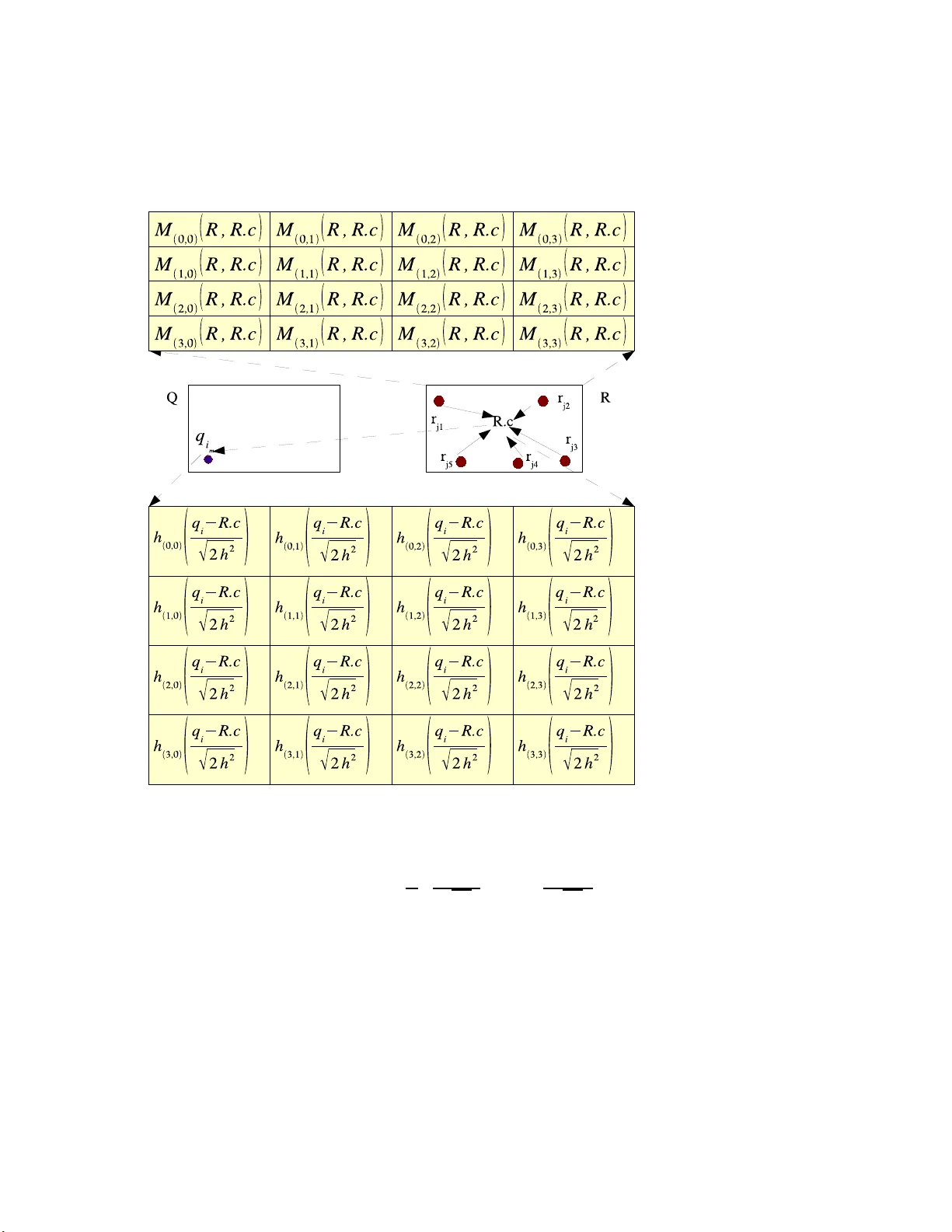
1 then H [ d ][1] ← 2 · a [ d ] · e − ( a [ d ]) 2 if p > 2 then for k = 1 to k = p − 2 do H [ d ][ k + 1 ] ← 2 · a [ d ] · H [ d ][ k ] − 2 · k · H [ d ][ k − 1] Implementing the lo cal-to-lo cal translation op erator. W e direct readers’ attention to the first step o f the algo r ithm, which r etrieves the ma ximum order among used in lo ca l momen t ac- cum ulation/trans lation. Then the a lgorithm pro c e eds with a doubly-nested for- lo op over the loca l moments applies Equation (27) . See Algor ithm 2 6. Ev aluating the lo cal expansion of the giv e n query no de. This function (see Algo rithm 27) is consis ted o f one outer-lo op ov er refer ence po ints and the inner-lo op ov er the lo cal moments up to p D terms, where p is the maximum approximation order used among the reference no des pruned via far-to- lo cal and direct lo cal accumulations for Q . References [1] A. Appel. An efficient pro gram for many-bo dy simulation. SIA M Journal on S cientific and Statistic al Computing , 6:85, 198 5. [2] J. Barnes and P . Hut. A Hierarchical O ( N log N ) F orce-Ca lculation Algorithm. Natur e , 324, 1986. [3] B. Baxter and G. Rous sos. A new erro r es tima te of the fast Gauss transfor m. SIAM Journal on S cientific Computing , 24 :2 57, 20 02. 42 Algorithm 22 ComputeHermiteFunction ( H, α ): Computes the Her mite function h α ( · ) using the pre-co mputed pa rtial deriv atives H . f ← 1 for d = 1 to D do f ← f · H [ d ][ α [ d ]] return f Algorithm 23 Ev al F arFieldExp ansion ( R, Q, p ): Ev aluates the fa r-field expansio n o f the given reference no de R up to p D terms. { Allo cate space fo r holding the partial deriv atives. } H d =1 , ··· ,D k =0 , ··· ,p − 1 ← 0 for each q i m ∈ Q do { Compute partial der iv atives up to ( p − 1)-th or der a long each dimension. } ComputeP ar tialDeriv a tives q i m − R.c √ 2 h 2 , p, H w ← 0 for i = 0 to i = p D − 1 do α ← P ositionToMul tiindex ( i, p ) f ← ComputeHermiteFunction ( H , α ) w ← w + M α ( R, R.c ) · f e G ( q i m , R F ( q i m )) ← e G ( q i m , R F ( q i m )) + w [4] J. L. Bentley . Multidimensiona l Binary Sea rch T rees used for Asso ciative Searching. Commu- nic ations of the ACM , 18:5 09–51 7, 19 75. [5] P . B. Callahan. De aling with Higher Dimensions: The Wel l- S ep ar ate d Pair De c omp osition and its Appli c ations . PhD thes is , Johns Hopkins University , Baltimore, Mar yland, 1 995. [6] A. Gray a nd A. Mo ore. Rapid ev aluation of multip le density models . A rt ificial Intel ligenc e and Statistics , 200 3. [7] A. Gray and A. Mo ore. V ery fast m ultiv ariate kernel density estimatio n via computational geometry. In Joint Stat. Me eting , 2003. [8] A. Gray and A. W. Mo ore. N- B o dy Pr oblems in Sta tistical Learning. In T. K. Leen, T. G. Dietterich, and V. T r e s p, editor s, A dvanc es in Neur al Information Pr o c essing Systems 13 (De- c emb er 2000) . MIT P r ess, 2001. [9] A. G. Gray and A. W. Mo ore. Nonpar a metric Densit y Estimation: T oward Computationa l T ra ctability. In SIA M International Confer enc e on Data Mining 2003 , 20 03. [10] L. Gr eengard a nd V. Rokhlin. A F ast Algo rithm for Particle Simulations. Journ al of Compu- tational Physi cs , 73, 1 987. [11] L. Gr eengard and J. Strain. The F ast Ga us s T r ansform. SIAM Journal of Scientific and Statistic al Computing , 12(1):7 9 –94, 1 991. 43 Algorithm 24 TransF arToLocal ( R, Q , p ): Implements Equation (22). H d =1 , ··· ,D k =0 , ··· , 2( p − 1) ← 0 ComputeP ar tialDeriv a tives Q.c − R.c √ 2 h 2 , 2 p − 1 , H for i = 0 to i = p D − 1 do β ← P ositionToMul tiindex ( i, p ) for j = 0 to j = p D − 1 do α ← P ositionToMul tiindex ( j, p ) f ← ComputeHermiteFunction ( H , α + β ) L β ( { ( R, T ( Q.c, p )) } ) ← L β ( { ( R, T ( Q.c, p )) } ) + M α ( R, R.c ) · f L β ( { ( R, T ( Q.c, p )) } ) ← ( − 1) | β | β ! L β ( { ( R, T ( Q.c, p )) } ) { L β ( Q.c, R D ( Q ) ∪ R T ( Q )) } β
Loading high-quality paper...
Comments & Academic Discussion
Loading comments...
Leave a Comment