Predictors of short-term decay of cell phone contacts in a large scale communication network

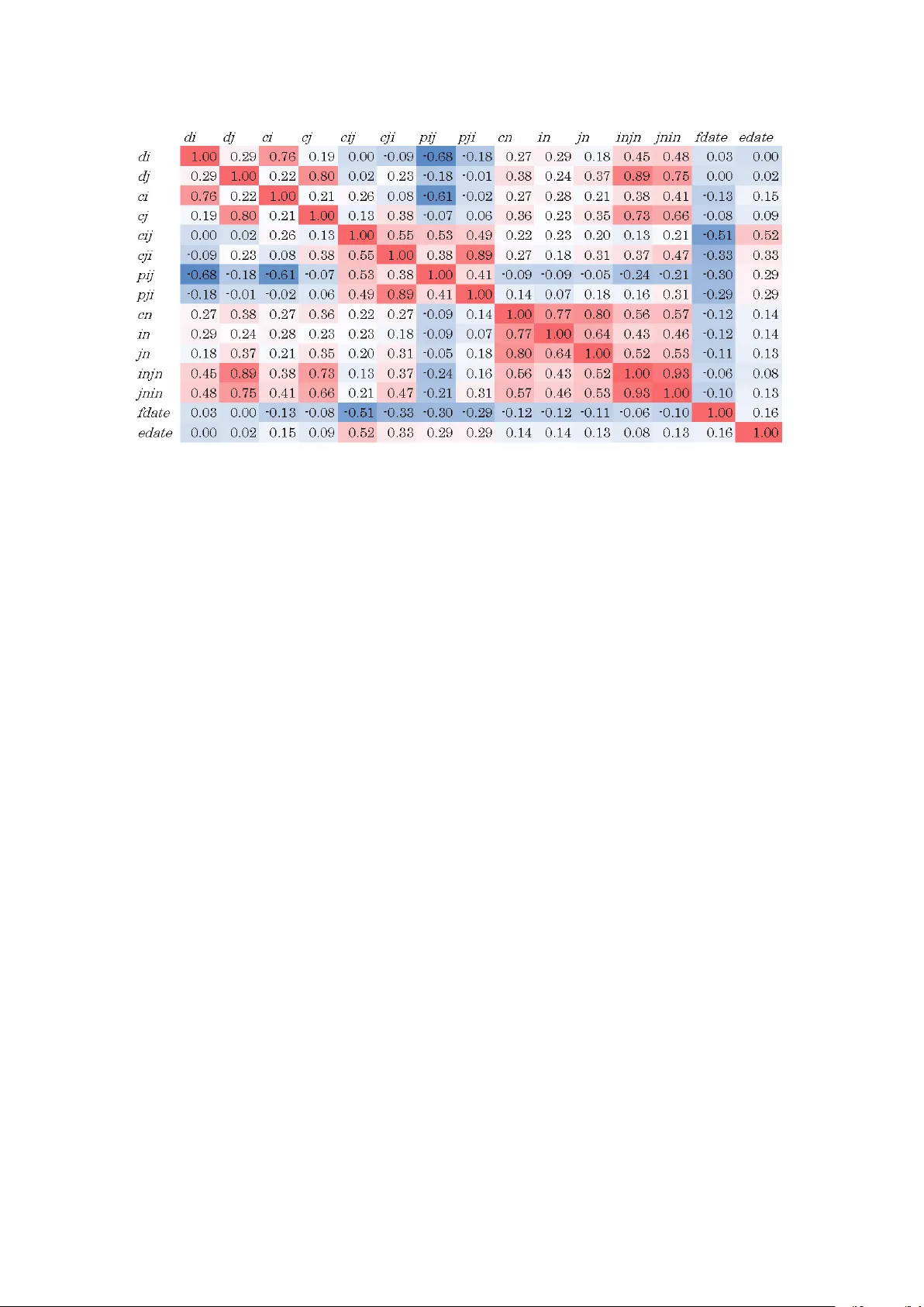
Predictors of short-term decay of cell phone contacts in a lar ge scale communication network I , II T roy Raeder a , Omar Lizardo b, ∗ , David Hachen b , Nitesh V . Chawla a a Deparment of Computer Science and Engineering, Colle ge of Engineering , University of Notr e Dame, 384 F itzpatrick Hall, Notr e Dame, IN, 46556 b Deparment of Sociology , University of Notr e Dame, 810 Flanner Hall, Notr e Dame, IN, 46556 Abstract Under what conditions is an edge present in a social network at time t likely to decay or persist by some future time t + ∆ t ? Previous research addressing this issue suggests that the network range of the people in volv ed in the edge, the extent to which the edge is embedded in a surrounding structure, and the age of the edge all play a role in edge decay . This paper uses weighted data from a large-scale social network built from cell-phone calls in an 8-week period to determine the importance of edge weight for the decay / persistence process. In particular , we study the relativ e predictiv e po wer of directed weight, embeddedness, newness, and range (measured as outdegree) with respect to edge decay and assess the e ff ectiv eness with which a simple decision tree and logistic regression classifier can accurately predict whether an edge that was activ e in one time period continues to be so in a future time period. W e find that directed edge weight, weighted reciprocity and time-dependent measures of edge longe vity are highly predictiv e of whether we classify an edge as persistent or decayed, relati ve to the other types of factors at the dyad and neighborhood lev el. K eywor ds: edge persistence, edge decay, link prediction, dynamic networks, embeddedness, tie strength, weighted networks 1. Introduction Under what conditions are particular social connections more or less likely to dissolve over time? Most network analysts agree that the issue of the dynamic stability of social rela- tionships embedded in networks is a fundamental one (Suitor et al., 1997; W ellman et al., 1997; Feld et al., 2007; Bidart I Research w as sponsored in part by the Army Research Laboratory and w as accomplished under Cooperativ e Agreement Number W911NF-09-2-0053 and in part by the National Science Foundation (NSF) Grant BCS-0826958. The views and conclusions contained in this document are those of the authors and should not be interpreted as representing the o ffi cial policies, either expressed or implied, of the Army Research Laboratory or the U.S. Gov ernment. The U.S. Government is authorized to reproduce and distribute reprints for Government purposes notwithstanding any copyright notation hereon. II W e would like to thanks the Social Networks editors and two anonymous revie wers for helpful comments and suggestions which served to significantly improve a pre vious version of this manuscript. ∗ Corresponding Author . and Degenne, 2005). One obvious reason for the centrality of relationship dynamics is that essentially all of the classic behavioral theories in the network tradition—such as balance (Heider, 1958; Da vis, 1963) and exchange theory (Emerson, 1972)—can be producti vely considered theories about the rela- tiv e likelihood that some edges will persist and other edges will be dissolved (Hallinan, 1978). For instance, classic balance- theoretic analyses of the dynamics of reciprocity suggest that the reason why we are more likely to observ e tendencies to- ward reciprocity in human social networks is precisely because unreciprocated edges hav e a shorter lifespan—they are more likely to be dissolved by the unreciprocated party—and are thus weeded out of the network through a selection process (Halli- nan, 1978; T uma and Hallinan, 1978; Hallinan and Hutchins, 1980; Hallinan and Williams, 1987; van de Bunt et al., 1999; van Duijn et al., 2003). A similar line of reasoning is behind Granov etter’ s (1973) influential “strength of weak edges” argu- Pr eprint submitted to Social Networks October 25, 2018 ment: the reason why the intransitiv e “forbidden triad” is rare, is precisely because dyads embedded in fully-reciprocated tri- ads are expected to be less likely to decay over -time (Davis, 1967)—a proposition that has received some empirical confir- mation by Burt (2000). While much attention has been paid to the emergence of transiti vity in social networks through a process of meeting through an intermediary , it is clear that thinking dynamically about the persistence of transitivity in social networks—through the selecti ve dissolution of relation- ships not embedded in triads—transforms this to a problem of accounting for the structural precursors of edge decay . This also implies that empirically “bridges” across transitive clus- ters should decay at a faster rate than other types of edges (Burt, 2002). In addition to these theoretical considerations, there are se v- eral substantiv e and practical motiv ations for the attempt to make progress in predicting edge persistent decay and persis- tence. First, at the level of the whole network, edge decay may signal changing community structure (T antipathananandh et al., 2007). From an ego-centric perspecti ve, if a gi ven actor e xperi- ences high-le vels of volatility and decay in her current relation- ships this may indicate that he or she is moving between peer groups or undergoing a major life change (Suitor and Keeton, 1997; Feld et al., 2007; Bidart and La venu, 2005). Second, rela- tionships that are identified as likely to decay may under some circumstances (e.g. when there is a need to binarize a weighted matrix) be better thought of as “false positiv es. ” In passiv ely- collected behavioral data such as email and cell phone com- munications (Kossinets, 2006; Hidalgo and Rodriguez-Sickert, 2008)—the source of data on which we rely in the analysis below—the notion of what exactly constitutes an edge is some- what unclear . Being able to predict edge decay may shed light on the circumstances under which an edge can be considered as “real” for the purposes of further analysis. More recently , with the increasing av ailability of longitudi- nal social network data, the temporal ev olution of social net- works is beginning to recei ve increasing attention (Burt, 2000, 2002; W ellman et al., 1997; Bidart and Degenne, 2005; Bidart and Lav enu, 2005). This has been aided by the recent de velop- ment of actor-oriented, stochastic approaches for the analysis of longitudinal network data (van de Bunt et al., 1999; Sni- jders, 2005) which couple the ev olution of micros-structures with agent-level attributes and behavioral outcomes (see Sni- jders et al. (2010) for a recent revie w). Howe ver , in spite of its centrality for the main lines of the- ory in network analysis, the dynamics of link decay remains a relativ ely understudied phenomenon, especially at the le vel of behavioral observ ation. In this respect, the main roadblock to a better understanding of the dynamics that dri ve patterns of de- cay of social edges in networks has been the relati ve paucity of large-scale, ecologically reliable data on social interactions (Ea- gle et al., 2008). The methodological and measurement issues associated with dynamic network data collected from informant reports on who they are connected to are well-kno wn and well- documented, so there is no need e xtensi vely rehearse them here (Bernard et al., 1984; Krackhardt, 1987). These include: (1) systematic measurement error introduced by constraints on va- lidity due to informant recall biases (Bre wer, 2000; Bre wer and W ebster, 2000; Marin, 2004), (2) measurement constraints in- troduced due to reliance on so-called fixed-choice designs to accommodate for respondent’ s memory limitations and stamina (Feld and Carter, 2002; K ossinets, 2006), and (3) validity lim- its introduced by data collection strategies that are limited (due to cost and the relativ e obtrusiveness of sociometric question- naires) to small samples constrained to specific sites (Laumann et al., 1989) (4) limitations in the ability to measure the volume and frequency of communicativ e acti vity that flo ws through an edge, with most studies being relegated to using standard bi- nary netw orks in which links are thought to be either present or absent (Opsahl and Panzarasa, 2009; Hammer, 1985). In the decay and formation dynamics of social relationships, these well-known limitations acquire rene wed importance for three reasons. First, as larg e-scale (sometimes containing thousands—and in our case millions—of actors) data on human communication begins to accumulate, examining the extent to which standard analytic approaches can be used to account for 2 empirical dynamics in this domain becomes a primary concern. Second, when considering the issue of link decay , the prob- lem of biases produced by memory limitations, artificial up- per bounds on actor’ s degree produced by survey design stric- tures and the selective reporting of those contacts most subjec- tiv ely (or objectively) important becomes an issue of substan- tiv e and methodological significance (Holland and Leinhard, 1973; K ossinets, 2006; Kossinets and W atts, 2006). For while it is unlikely that persons will misreport being connected to those with whom they interact most often (Hammer, 1985; Freeman et al., 1987), by selectively collecting data on ego’ s strongest edges, it is likely that surve y-based methods may give undue consideration to precisely those links that are least likely to de- cay . Finally , ignoring the f act that most real-world communica- tion networks are not binary—each edge is instead “weighted” di ff erently depending on the amount of communicati ve acti vity that flo ws through it (Barrat et al., 2004)—can impose artificial limits on our ability to predict which links are more lik ely to de- cay and which ones are more likely to remain. In this paper we use behavioral network data on a large-scale sample of commu- nicativ e interactions—obtained unobtrusiv ely from cell-phone communication records—to study the dynamic and structural processes that govern link decay . One adv antage of the data that we use below is the fact that it consists of weighted links based on dyadic communication frequency It is of course not our intention to suggest that data obtained from cellular communication records are themselves de void of bias or that pre vious research using self-report data do not con- stitute a solid foundation on which to build. In fact, we rely on research and theory from such studies in the analysis that follows. Cellular communication data are certainly not a direct reflection of the underlying social network. Communicating by phone is only one out of a large menu of possible ways in which two persons may be connected; and in fact may persons can share strong connections without necessarily talking over the phone. In addition just like informants may fail to mention their least important ties, rare-behavioral ev ents (e.g. contact- ing somebody whom you only talk to once a year) will also be absent from observational data unless really long observation windows are used, thus producing a similar observ ational bias keyed to relati ve strength. It is our contention howe ver , that data obtained from sponta- neous behavioral interactions will produce dynamical patterns that may be closer to those that govern the formation, suste- nance and decay of human social relationships in “the wild” (Hammer, 1985). As such, they are an important resource to establish the structural and dynamic properties of lar ge-scale social networks.W e already know that data of this type have high ecological validity , in that cell-phone mediated interaction accurately predicts face-to-face interaction and self-reported friendship as measured using traditional sociometric methods (Eagle et al., 2009). With penetration rates close to 100% in industrialized countries such as the one from which these data were collected (Onnela et al., 2007), cell-phone communica- tions are also generally dev oid of the socio-demographic biases that plagues studies that rely on modes of communication that hav e yet to achieve comparable le vels of uni versal usage (such as email or chat). Onnela et al. (2007) examined basic topolog- ical properties of a cell-phone communication network similar to ours, and found it to display some basic signatures specific to social networks (e.g. small mean-path length, high-clustering, community structure, large-inequalities in connecti vity across vertices, etc.). This paper makes several contributions to the literature. First, on the substantiv e side, we incorporate insights and mecha- nisms from previous studies of network e volution to understand processes of link decay . In addition we bring into considera- tion dyad-le vel process–such as de gree of reciprocity–that ha ve not yet been considered in studies of edge decay (mostly due to the fact that the data used are binary and not weighted). On the methodological side, we introduce supervised learning tech- niques from the computer science literature for the study of so- cial network ev olution. These techniques are appropriate for discov ering patterns in data of the size and scope with which we are faced here (millions of persons and tens of millions of communication events), both extending and complement- 3 ing the more traditional regression-based techniques that have been used to tackle this problem in the existing literature (e.g Burt, 2000, 2002). Machine learning algorithms allo w us to as- certain the relati ve importance of individual, dyadic and local- structural information in contributing to lowering or increasing the likelihood of link decay without incorporating strong as- sumptions about functional form—they are “non-parametric” in this respect—or homogeneity of e ff ect sizes across the rele- vant feature space. The remainder of the paper is organized as follows: In the following section we briefly revie w previous research on edge decay in social networks. In Section 3 we connect the substan- tiv e concern with identifying the factors that lead to link decay in the social networks with the lar gely methodological literature related to the link prediction problem in computer science and explain how we partially adapt these tools to the task at hand. In Section 4 we go on to revie w previous work on the dynam- ics of social relationships in large-scale networks. In Section 5 we describe the data on which we conducted this study and for - mally define each of the problems we consider . Section 7 de- scribes basic topological and distrib utional features of our main predictors. In Section 8 we examine the correlation structure among the network features that we choose for the prediction task. In Section 9 we present the results, identifying which net- work features are the strongest predictors of edge decay . In Section 10 we analyze the classifier’ s performance and explore their comparative fit. Finally in Section 11 we discuss the sub- stantiv e implications of our results, draws conclusions, and lay out potential av enues for future research. 2. Correlates of Edge Decay in Social Networks A great deal of e ff ort has gone into characterizing the growth of netw orks, either with high-le vel generati ve models (see (Chakrabarti and Faloutsos, 2006) for a survey) or by analyz- ing the formation of individual links (Hays, 1984; Marmaros and Sacerdote, 2006). Comparativ ely little work has been done on decay dynamics in large-scale networks with an already ex- isting structure: the processes by which individual actors leave the network or individuals sev er edges. The most exemplary work on the issue of edge decay in social networks is that of Burt (2000, 2002), who studies the social networks of promi- nent bankers over time and analyzes the factors that contribute to the disappearance of edges. Specifically , prominent bankers within an organization were asked, once a year for four years, to name other bankers from the same organization with which they had had “frequent and substantial business contact” over the previous year . T wo main substantiv e conclusions emerge from this analysis: 1. Sev eral factors influence edge decay , including homophily (similarity between people), embeddedness (mutual ac- quaintances), status (e.g. network range), and experience. 2. Links exhibit a “liability of newness”, meaning that newly- formed links decay more quickly than links that hav e ex- isted for a long time. These observations seem to lay out a frame work for predict- ing link decay (and by implication, link persistence), and that is precisely the chief question of this paper: What are the vertex- level, dyad-level and local-structural features that can be used to most accurately pr edict edge decay? A formal statement of this research question giv es rise to what we will call the decay pr ediction problem: Giv en the activity within a social network in a time period τ 1 , how accurately can we predict whether a giv en edge will persist or decay in a follo wing window τ 2 ? In what follo ws we ev aluate the e ff ecti veness of a machine learn- ing solution to the decay prediction problem. 3. The Link Prediction Pr oblem The problem of decay prediction is intimately related to the link pr ediction problem. There are sev eral related but slightly di ff erent problems that are termed “link prediction” in the com- puter science literature. The most related one, originally studied by Liben-Nowell and Kleinberg (2007) can be stated as follows: giv en the state of a network G = ( V , E ) at time t , predict which new edges will form between the vertices of V in the time inter - val τ = ( t , t + ∆ t ). See (Bilgic et al., 2007; Clauset et al., 2008) 4 for additional work in this vein or (Getoor and Diehl, 2005) for a surve y . Other authors (Kashima and Abe, 2006) ha ve formulated the problem as a binary classification task on a static snapshot of the network, but this version of the problem is less related to the present e ff ort simply because it is not longitudinal in na- ture. Current research on link prediction in computer science focuses mostly on ev aluating the ra w predicti ve ability of di ff er- ent techniques, by either incorporating di ff erent vertex and edge attributes (O’Madadhain et al., 2005; OMadadhain et al., 2005; Popescul and Ungar, 2003) or the selecting di ff erent learning methods (Hasan et al., 2005) in order to improve prediction per- formance. Where we di ff er from this work, apart from address- ing a slightly di ff erent problem, is that we attempt to system- atically characterize the attributes that lead to successful clas- sification. In other words, rather than being concerned simply with whether , or to what extent, our models succeed or fail, we attempt to characterize why they are successful or unsuccess- ful by measuring the importance of di ff erent attributes and of weighted edge data to classification. 4. Pre vious longitudinal resear ch on large-scale networks Sev eral authors have studied the e volution of large networks and identified characteristics that are important to the forma- tion of edges. K ossinets and W atts (2006) studied the ev olu- tion of a Uni versity email network over time and the extent to which structural properties, such as triadic closure, and ho- mophily contribute to the formation of ne w edges. Of particular relev ance to us, they find that edges that would close triads are more likely to form than edges that do not close triads, and that people who share common acquaintances are much more likely to form edges than people who don’t. Similarly , Lesko vec et al. (2008) study the evolution (by the arriv al of vertices and the formation of edges) of four large online social networks and conclude, among other things, that triadic closure plays a very significant role in edge formation. Both of these factors are re- lated to the notion of embeddedness which we study in the con- text of edge decay , but neither of these authors consider edge decay at all. Marsili et al. (2004) develop a model for network ev olution that allows for the disappearance of edges, but they do not validate the model on any real-world data. As a result, the extent to which social networks fit the model is unclear and it does not shed any light on the mechanisms behind edge decay . The e ff ort that is closest to ours in principle is a paper by Hi- dalgo and Rodriguez-Sickert (2008), which analyzes edge per- sistence and decay on a mobile phone network very similar to our o wn. Howe ver , the analysis undertaken below di ff ers criti- cally from theirs both in methodology and primary focus. The aforementioned paper relies on a highly circumscribed set of well-established physical network statistics (i.e. degree, clus- tering coe ffi cient) as well as reciprocity to explain decay . In what follows, we consider time-dependent properties of edges (Burt, 2000) as well as features associated with interaction fre- quency (edge weight) (Marsden and Campbell, 1984; Hammer, 1985; Barrat et al., 2004). 5. Data and features 5.1. Data Our primary source of data in this study consists of informa- tion on millions of call records from a large non-U.S. cell phone provider . The data include, for each call, anonymized informa- tion about the caller and callee (i.e. a consistent index), along with a timestamp, duration, and the type of call (standard call, text message, voicemail call). Our original dataset is composed primarily of phone calls and text messages. In the empirical analysis that follows, ho we ver , we restrict ourselves to dyadic communications that take the e xclusive form of a voice call (we exclude text messages). W e exclude all vertices with more that fifty neighbors, to ensure that only persons (and not auto-dialing robots) are represented in our data. Our final dataset consists of all in-network phone calls made ov er a 8-week period in 2008. W e restrict our attention to in- network calls (where both the caller and callee use our provider) because we only have information about calls initiated by our provider’ s customers. That is to say , if i is on the network but j 5 Statistic V alue A verage Clustering Coe ffi cient ( d i > = 2): 0.24 Median Clustering Coe ffi cient: 0.14 A verage Out-Degree: 4.2 Median Out-Degree: 3 A verage T otal Degree: 6.3 Median T otal Degree: 3 Number of V ertices: 4,833,408 Number of Edges: 16,564,958 T able 1: Basic graph-statistics of the cell-phone network. is not, we kno w if and when i calls j , b ut not if and when j calls i . In order to accurately predict the decay of edges, we need to be able to capture the degree of r ecipr ocity in the relationship, meaning we need to be able to see if and when j calls i back. Thus, we only examine edges where both i and j use our cell phone provider . 5.2. Connectivity Criterion Naturally , we represent this information as a directed social network, where the vertices are the individual subscribers. An edge exists from actor i to actor j if i has at least one v oice communication with j during an initial window τ 1 = ( t , t + ∆ t ), which we define as τ 1 = 4 week s . Using this connectivity criterion, we identify approximately 16.5 × 10 6 directed edges in the network (see T able 1). Edges can be either bi-directional or directed arcs, depending upon whether j made a call back to i during τ 1 . T able 1 shows some basic topological statistics of the observed graph. 5.3. F eatures Using the connectivity structure of the network constructed from the first four-weeks of data, we extract a number of vertex- lev el, dyad-le vel and higher-order features based on the intu- itions provided by previous research and theory on relationship dynamics (e.g. Hallinan, 1978; Burt, 2000; Feld et al., 2007), especially as they pertain to behavioral networks with weighted edges (Hammer, 1985; Barrat et al., 2004). These features are giv en in T able 2 and can be grouped into four categories or sets: verte x, dyadic, neighborhood, and temporal features. 1 5.3.1. V ertex-level featur es The vertex-le vel features include the outde grees of i and j ( d i and d j ), and the overall communicative activity of each verte x ( c i and c j ), that is the overall number of calls made by each member of the dyad during the 4-week time period, respec- tiv ely . 5.3.2. Dyad-level featur es The dyadic level features include the directed arc strength, i.e. the counts of the number of voice calls made by i to j ( c i j ), and the number of calls made by j to i , c i j . W e also compute normalized v ersions of arc strength ( p i j and p i j ) which are sim- ply the proportion of all calls made by an agent that go to that neighbor , where p i j = c i j / c i . 5.3.3. Neighborhood-level featur es The neighborhood-lev el features include (1) the number of common neighbors between i and j ( cn ), (2) directional ver- sions of the number of common neightbors ( in and jn ) which indicate the number of i ’ s (or j ’ s) neighbors that called j (or i ), and (3) second order embededness features ( in jn and jnin ) 1 W e do not include any homophily-based features in this analysis, as we do not yet hav e reliable customer demographic information for the time period in question. 6 which measure the number of edges among i and j ’ s neighbors. in jn does this by counting as an edge calls made from one of i ’ s neighbors to one of j ’ neighbors, while jnin considers an edge as existing when one of j ’ neighbors calls one of i ’ s neighbors. 5.3.4. T emporal featur es Finally we look at two features related to the (observed) tem- poral evolution of dyadic communicati ve behavior: f d ate cap- tures edge newness as indicated by the time of the first call from i to j during our temporal window τ ; f d ate marks far into our time window , τ , we first observe a call from i to j . Higher val- ues indicate newer edges, while smaller values indicate older edges. The second temporal feature, ed ate , captures the edge fr eshness as indicated by the time of the last call made by i to j , giv en that the edge has already been observed to exist. Higher values indicate that the edge was acti ve in the more recent past, while smaller v alues indicate that the edge has been inactive for a longer period of time. T o the best of our kno wledge, prior work has not consid- ered the freshness of an edge as a predictor of persistence / decay , though edge ne wness has been seen as as an important predic- tor of short-term decay via Burt’ s isolation of the phenomenon of the “liability of newness” of social ties (Burt, 1997, 2000). W e believe that the freshness of an edge could be an important predictor as it indicates ho w current the edge is and we expect that more current edges are more relev ant in the immediate fu- ture. If persistence or decay are partly a markov process with a relativ ely short memory , then edge-freshness should emer ge as an important predictiv e factor . 5.4. Edge-decay and edge-per sistence criterion W e use these features to build a model for predicting whether edges fall into two disjunctive classes: persistent or decayed . For the purposes of this analysis an edge is said to persist if it is observed to exist in the time period τ 2 = ( t +∆ t , t +∆ t +∆ t 0 ) giv en that it was observed in the previous time period τ 1 = ( t , t + ∆ t ) using the same connectivity criterion outlined in section 5.2 abov e. Con versely , an edge is said to have decayed if it was observed to exist in τ 1 = ( t , t + ∆ t ) b ut it can longer be detected in τ 2 = ( t + ∆ t , t + ∆ t + ∆ t 0 ) using the same operational crite- rion. 2 Note that the observ ation and criterion periods are e venly divided such that τ 1 = τ 2 = 4 week s (see Figure 1). 6. Machine-Learning models f or the edge-classification problem Having obtained a set of structural features from the network built from the information observed in τ 1 , our final task is to build a model that will allows us to most e ff ecti vely assign each edge to either the persistent or decayed class using the criterion outlined in section 5.4 abov e. Giv en the large scale of our com- munication network, we turn to methods from data-mining and machine-learning to accomplish this task. W e proceed by arranging the av ailable data as a set of in- stances or examples , each of which is observed to belong to a given class, which in our case is either persistent or decayed. As we noted abov e, associated with each instance is a set of fea- tur es or attributes . The task is to build a generalizable model from the a v ailable data. In our case, since our class takes only the value 0 (decayed) or 1 (persistent), we need to deriv e a func- tion F : x → { 0 , 1 } which predicts (with some ascertainable accuracy) the class of an attrib ute given a v ector of features X . After building the model, we need to validate its e ff ectiv e- ness on a set of instances that are di ff erent from those used to build the model. T ypically this is done by di viding the av ailable data into two disjoint subsets (the horizontal line in Figure 1). The first subset, called the training data , is used to build the model. Once the model is built, we use it to predict the class of each instance in the test data. The e ff ecti veness of the model, 2 W e believe that a 4 week period is a long enough time window for deter- mining edge persistence / decay at least in the short to medium term. While tech- nically an edge could be inacti ve during this period and reappear afterwards, all indications are that very few edges are like this, and those that are are very weak and fleeting. While we could have lengthened the τ 2 time period, this would have meant shortening the τ 1 period, but doing so would have a ff ected our estimates of edge features that we use in the analysis. Giv en that we have a total time window of τ 1 + τ 2 = 8 week s , we decided that the best strategy is to divide the period in half and define decay as the non-occurrence of voice calls between i and j in the second time period. 7 Figure 1: Diagram of the data-splitting procedure used to generate basic features and to determine dyadic class-membership in the analysis below . then, depends on its accuracy (or some other measure of per- formance) on the test data. As sho wn in Figure 1, the data are split within each time period ( τ 1 , τ 2 ) into training and test sub- sets. In the analysis reported below , we randomly designated 2 / 3 of the original examples in the data in the first period to the training set and used the remaining 1 / 3 of the data as the testing set. The figure also shows the number of dyads in testing and training set that ended up in the decayed class (about 43%). 6.1. The decision-tr ee classifier There are a number of potential models av ailable for ev alu- ating the e ff ecti veness of our chosen features at predicting edge decay . Perhaps the simplest of these, which was used in Burt’ s analysis (Burt, 2000), is simple regression: plotting each fea- ture as the independent variable against the probability of de- cay . Such an approach has the distinct advantage that it is easy to interpret. Regression is of course one of many classification tools a v ailable and also has the adv antage of relati ve ease of in- terpretation. In what follows we present results obtained from both a logistic regression classifier (which provides easily inter - pretable output that can be compared with previous research on the subject) and a decision-tree classifier which is an approach that has not been used very often in the analysis of Social Net- works. 3 While relativ ely unfamiliar in the analysis of social networks, the decision tree is the most well-known and well- researched method in data-mining and provides output that is easily translatable into a set of disjoint “rules” for (probabilis- tically) assigning di ff erent cases to one of the two outcomes. In our case we are interested in what combination of features maximize either edge decay or edge persistence. Because read- ers may not be wholly familiar with the decision-tree classifier approach, we provide a brief introduction to the basics of the approach before presenting the results. W e presume that read- ers are familiar with the basics of logistic re gression so we will not discuss it in detail. A decision tree classifies examples with a hierarchical set of rules. A decision tree model is built by recursi vely dividing the feature space into pur er (more discriminating) subspaces along 3 An important consideration with machine learning methods, as with sta- tistical methods, is the choice of model to which we attempt to fit the data. A nearly boundless series of models has been developed in the literature (W itten and Frank, 2005), and a discussion of the merits of each is well beyond the scope of this paper. Instead, we will discuss one of the models we chose (a decision tree model called C4.5 (Quinlan, 1993)) and its relative strengths for the problem at hand. 8 (a) (b) Figure 2: (a) T oy classification dataset. (b) Resulting decision tree splits that are parallel to the feature axes. A very simple exam- ple is shown in Figure 2. Giv en the task of classifying unknown points as either blue circles or red squares (Figure 2(a)), a deci- sion tree trained on the data points shown will produce a series of splits along the two dimensions in the figure ( x and y ). Gen- erally , the first split is along whichev er attribute is deemed to be the best separator of the classes according to some measure. Our implementation of C4.5 determines the “best” split using information gain (which we will formally define in Section 9 below). Our hypothetical decision tree makes its first split along the line down the middle of the figure ( x = 5) A tree induction algorithm will then recursi vely di vide up each of the resulting subspaces until some stopping criterion (i.e. a minimum number of instances per leaf or minimum leaf purity) is met. Figure 2(b) shows the decision tree gen- erated by the splits corresponding to the “data” in the left-hand side. Unkno wn instances are classified by taking the appro- priate branches of the tree until a leaf is reached. The class assigned to the unkno wn instance is whichev er class was most common among the training instances at that leaf. The Figure shows that any instance with x > 5 and y > 10 is classified as a red square, while e verything else is a blue circle. The pri- mary adv antage of decision trees for our decay prediction task (besides, of course, reasonable performance) is interpr etability . Examining the classification accuracies at the individual leaves, we can see where the model is strong and where it is weak. Ad- ditionally , decision trees enable us to sho w that the importance of the features defined in T able 2. 6.2. Outline of the empirical analysis In what follows, we consider the following three empirical issues within our chose time window ( τ ): 1. F eature corr elation : In the initial time window τ 1 = ( t , t + ∆ t ), what is the correlation structure of the features sho wn in T able 2 ? 2. F eature pr edictiveness : Having observed the network in a time window τ 1 = ( t , t + ∆ t ), which features of the network are most predicti ve of the class membership of each edge (persistent / decayed) in the adjacent time windo w τ 2 = ( t + ∆ t , t + ∆ t + ∆ t 0 )? 3. Edge-class Pr ediction : Giv en a set of feature-predictors from the initial time windo w τ 1 = ( t , t + ∆ t ), can we build a model that accurately predicts the class membership of the edges observed in the following time window τ 2 = ( t + ∆ t , t + ∆ t + ∆ t 0 )? After briefly considering some basic descripti ve statistics on each of the predictor features in the next section, in section 8 we shed light on the first question by examining the pairwise Spearman correlation coe ffi cients ( ρ ) among all pairs of fea- tures in T able 2; in section 9 we address the second question 9 0 10 20 30 40 50 0 0.5 1 1.5 2 2.5 x 10 6 d1 count (a) Outdegree of i 0 10 20 30 40 50 0 0.5 1 1.5 2 2.5 x 10 6 d2 count (b) Outdegree of j 10 0 10 1 10 2 10 3 10 4 10 0 10 1 10 2 10 3 10 4 10 5 10 6 c1 count (c) N. of calls made by i 10 −1 10 0 10 1 10 2 10 3 10 4 10 0 10 1 10 2 10 3 10 4 10 5 10 6 c2 count (d) N. of calls made by j 0 0.2 0.4 0.6 0.8 1 10 0 10 1 10 2 10 3 10 4 10 5 10 6 10 7 cci count (e) Calls from i to j 10 −1 10 0 10 1 10 2 10 3 10 4 10 0 10 1 10 2 10 3 10 4 10 5 10 6 10 7 cji count (f) Calls from j to i 0 0.2 0.4 0.6 0.8 1 10 0 10 1 10 2 10 3 10 4 10 5 10 6 10 7 pij count (g) Prop. of i → j calls 0 0.2 0.4 0.6 0.8 1 10 0 10 1 10 2 10 3 10 4 10 5 10 6 10 7 pji count (h) Prop. of j → i calls 0 10 20 30 40 50 10 0 10 1 10 2 10 3 10 4 10 5 10 6 10 7 cn count (i) N. of common neighbors 0 5 10 15 20 25 30 35 40 10 0 10 1 10 2 10 3 10 4 10 5 10 6 10 7 in count (j) N. of i s neighbors that call j 0 5 10 15 20 25 30 35 40 10 0 10 1 10 2 10 3 10 4 10 5 10 6 10 7 jn count (k) N. of j s neighbors that call i 0 50 100 150 200 250 300 10 0 10 1 10 2 10 3 10 4 10 5 10 6 10 7 injn count (l) N. of calls from i → j ’ s neighbors 0 50 100 150 200 250 300 10 0 10 1 10 2 10 3 10 4 10 5 10 6 10 7 jnin count (m) N. of calls from j → i ’ s neighbors 10 7.7 10 7.71 10 5 10 6 10 7 fdate count (n) Time of first call from i to j 10 7.7 10 7.71 10 5 10 6 10 7 edate count (o) Time of last call from i to j Figure 3: Cumulativ e distributions of the features included in the analysis. 10 Feature Description Range Median verte x Le vel d i Out degree of i (Ego-network Range) 1-49 2 d j Out degree of j (Ego-network Range) 0-49 1 c i Number of calls made by i (gregariousness) 1-1366 22 c j Number of calls made by j (greg ariousness) 0-1366 22 Dyad Lev el c i j Calls from i to j (directed edge strength) 1-1341 2 c ji Calls from j to i (reciprocated edge strength) 0-1341 1 p i j Proportion of i s calls that go to j ( c i j / c i ) 0-1 0.15 p ji Proportion of j s calls that go to i ( c ji / c j ) 0-1 0.08 T riad Level cn Number of common neighbors between i and j (edge embededness) 0-46 0 in Number of i s neighbors that call j (directed edge embededness) 0-39 1 jn Number of j s neighbors that call i (directed edge embededness) 0-39 0 in jn Number of calls that i ’ s neighbors make to j ’ s neighbors (2nd order embededness) 0-274 7 jnin Number of calls that j ’ s neighbors make to i ’ s neighbors (2nd order embededness) 0-274 6 temporal f dat e Normalized time of first call from i to j (edge ne wness) 0-1 0.26 ed ate T ime of last call from i to j (edge freshness) 0-1 0.74 T able 2: List of features to be used in predicting edge persistence / decay i → j . using an information-theoretic measure of randomness for pre- dicting short-term decay . Finally Section 10 addresses the fi- nal question by formulating the edge-decay prediction task as a binary classification problem using a machine learning data analysis strategy . 7. Featur e statistics The range and median values on the features are computed based on data from the first 4 week time period and summary statistics are provided in T able 2. As sho wn in Figure 6.1 of the distributions are highly ske wed with substantially more lower than higher values so we report medians. As noted earlier we omit edges with vertices which have degrees greater than or equal to 50 in order to eliminate robot calling, so vertex degree ranges from 1-49. Note that we ha ve included asymetric edges, that is edges in which i called j during τ 1 , but j did not return a call during that time period, so there are nil values for d j , c j , and c ji . During this τ 1 period the median outde gree for the focal ver - tex i is 2, but for its paired vertex j 1 because of the presence of asymmetric edges in which d out i > 0 and d out j = 0. The me- dian value for the number of calls made by subscribers is 22. At the dyad level, the median number of calls from i to j is 2, but from j to i it is 1, again because of asymmetric edges. c ji , therefore should be vie wed as an indicator or reciprocity in that it indicates the extent to which vertex j makes calls to i giv en that i made at least one call to j . p i j and p ji are normalized versions of c i j and c ji respectiv ely and indicate what proportion of the total calls made by the i th subscriber went to each of its j neighbors. The median v alue of p i j of 0.15 indicates that for 11 Figure 4: Spearman Correlation ( ρ ) between pairs of features in one week of call data. the edge at the middle of the p i j distribution about 15% of its total calls went to its neighbor . T urning to the neighborhood-lev el features, the vertices joined by the median edge do not share a common neighbor as indicated by the median v alue of 0 for cn . There appears to be a good deal more embeddedness when we measure it in terms of the edges between i and j ’ s neighbors instead of directed edges from i ’ s (or j ’ s) neighbors to j (or i ); the neighbors of vertices joined by the median edge are expected to make about seven calls to one another . Finally for the two temporal features we hav e normalized them so their v alues range from 0-1. V alues on f dat e and ed ate indicate where, in the 4 week time period, the relev ant ev ents occurred. For f d ate , the newness of the edge, the median value is .26 indicating that 50% of the edges were activ e (a call had been made from i to j ) at or before about one week had elapsed. For ed ate , the freshness of an edge, the me- dian value of .74 indicates that for 50% of the edges the last call was made by i to j before three weeks had transpired. 8. Featur e correlations Figure 4 shows the Spearman correlations that capture the association between features during the first four week time pe- riod. A number of very strong correlations (shaded red—for positiv e correlations—and blue—for negativ e correlations—in the figure) are immediately apparent. Among the vertex le vel features, degree ( d i or d j ) and gregariousness ( c i or c j ) are highly correlated (.76 and .80) indicating that vertices with more neighbors make more calls. Among the dyadic lev el fea- tures the normalized and raw features of directed edge weight are correlated gi ven that the normalized measure ( p i j ) is a func- tion of the raw measure ( c i j ). The correlation between c i j and c ji is positiv e indicating the presence of reciprocity , that is as the number of calls from i to j increases so does the number of calls from j to i . Ho we ver this correlation is not extremely high, indicating that dyads do vary in their lev el of reciprocity . Among the neighborhood-lev el features, the correlations are positiv e and for the most part large, which could indicate that the simplest measure of embeddedness, the number of common neighbors ( cn ), is a good enough measure and one does not need to look at directional or second-order embeddedness. Finally it is interesting to note that the two temporal features, f dat e and ed ate , are independent. edges that are relativ ely older (i.e. a call occurred earlier in the 4 week time period) can be more or less current. Looking at the correlations acr oss the various categories of the features, what is striking is how low they are. For the most 12 Featur e Description Info. Gain d i Degree of i . 0.00235 d j Degree of j . 0.00234 c i Calls made by i . 0.01181 c j Calls made by j . 0.00449 c i j Calls from i to j . 0.17948 c ji Calls from j to i . 0.12823 p i j Proportion of i ’ s calls that go to j 0.13318 p ji Proportion of j ’ s calls that go to i . 0.12043 in Number of i ’ s neighbors that call j . 0.02478 jn Number of j ’ s neighbors that call i ’ s neighbors. 0.02303 cn Number of common neighbors between i and j . 0.02441 jnin Number of j ’ s neighbors that call i ’ s neighbors. 0.01501 in jn Number of i ’ s neighbors that call j ’ s neighbors. 0.00493 f dat e T ime of first call from i to j . 0.05104 ed ate T ime of last call from i to j . 0.09954 T able 3: Information gain of each feature for predicting short-term edge decay using four weeks of data. The information gain measures the conditional ability of that feature to predict edged decay in the subsequent week within lev els of the other features. part verte x, dyadic, neighborhood and temporal features are in- dependent from each other . One exception to this pattern is the correlation between outdegree ( d i or d j ) and the normal- ized edge weight features, p i j or p ji . This has to be the case because the sum of the p i j ’ s for a giv e i is 1, so the more neigh- bors a person has, the lower the proportion of their calls going to each neighbor must be (the so-called bandwidth / range trade- o ff (Aral and V an Alstyne, 2007)). Another exception to the pattern of low correlations between features in di ff erent cate- gories, is the high correlations between outde gree (and gre gari- ousness) and the second order embeddedness features, in jn and jnin . Agents that have more neighbors are also going to hav e more edges between their neighbors and the neighbors of the other vertices to which the y are connected. As such our second order embeddedness features essentially reduce to indicators of verte x range. Finally , the two “temporal” features, f d ate and ed ate are correlated with edge weight ( c i j and to a less extent c ji ). Recall that f d ate features the newness of an edge and that lower values are indicati ve of older edges. The negati ve corre- lation of f d ate with c i j indicates, therefore, that newer edges are weaker and older edges are stronger . The positive correla- tion of ed ate with c i j indicates that fresher edges (i.e. edges in which a call has been made more recently) are also stronger . In sum, it appears that there are really four relativ ely indepen- dent sets of edge features pertaining to verte x, dyadic, neighbor- hood and temporal levels. While there are multiple indicators within each of these sets, they tend to be highly correlated, with the exception of the two ”temporal” features. Though in the re- mainder of the paper we will be looking at the predictiv e v alue of all these features, based on these correlations our focus will be on the follo wing potentially important features: outdegree (both d i and d j ), edge weight ( c i j ), reciprocated edge weight ( c ji ), the number of common neighbors ( cn ), and both the ne w- ness of the edge ( f dat e ) and its freshness ( edat e ). 13 9. Featur e Predictiveness W e wish to determine the extent to which each of the above features as observed in the first time window helps us classi- fies edges as either decayed or persistent in the following time- window . By determining this, we can quantify , to some extent, the usefulness of the features for decay prediction. There are sev eral possible indicators of predictive ability . Here we rely on the information gain , which is the standard measure of fea- ture predictiveness in data-mining (Witten and Frank, 2005). Approaches to determine the importance of predictors based on information theory are common in statistics (Menard, 2004; Gilula and Haberman, 2001). Information-theoretic approaches hav e been applied before in the characterization of overall struc- tural features of social networks (e.g. (Butts, 2001; Leydes- dor ff , 1991); here they are deployed in the interest of quantify- ing the predictiv e ability of fine-grained (local) structural fea- tures for the link prediction problem. 9.1. F ormal definition of Information Gain Information gain tracks the decrease in entr opy associated with conditioning on an attribute, where entropy is a measure of the randomness (alternately , predictability) of a quantity . T o understand the measure and how it quantifies feature impor- tance, consider as an example our two-class cell phone dataset, where each edge is either persistent (class 1) or decayed (class 0). If we define p ( x ) as the proportion of instances of class 1 and q ( x ) as the proportion of class zero, the entropy H ( x ) is defined as: H ( x ) = − p ( x ) log p ( x ) − q ( x ) log q ( x ) (1) where all logarithms are taken to base 2. If the two classes are perfectly balanced, then the entropy H ( x ) = log 2 = 1. As the classes become increasingly imbalanced, the entropy de- creases. That is to say , we know more a priori about the class of a random instance. If a particular feature is informati ve, then conditioning on that feature should decrease the entropy of the dataset. Suppose, for example, that a feature F takes a set K of possible values. The conditional entr opy of the dataset condi- tioned on the feature F is: H ( x | F ) = X k ∈ K − p k ( x ) log p k ( x ) − q k ( x ) log q k ( x ) (2) Where p k ( x ) = p ( cla s s = 1 | F = k ) is the proportion of positiv e-class instances among the instances where the fea- ture F takes the value k . Similarly , q k ( x ) is the proportion of negati ve-class instances. The information gain for the feature F is the decrease in entropy achiev ed by conditioning on F : I ( x | F ) = H ( x ) − H ( x | F ) | K | . Returning to our hypothetical example, suppose there is a feature F that takes on two values: A and B . Instances with F = A are 90% class 1 and instances with F = B are 90% class 0, then I ( F ) = log 2 − ( − 9 10 log 9 10 − 1 10 log 1 10 ) = 0 . 530 . The information gain I ( x | F ) has an appealing intuiti ve interpre- tation as the percentage of information about the class that is rev ealed by the feature F . By calculating the information gain of each feature in T able 2, we can determine which actor and edge attributes re veal the most information about edge decay . 9.2. F eature Importance in the Call Network T able 3 shows the information gain of each feature described in T able 2 calculated for the first four weeks of data. The re- sults show that the four most predictive features are dyadic features of directed tie strength as gi ven by the frequency of interaction and the extent to which communications are con- centrated on a giv en alter: number of calls sent and received along the edge ( c i j and c ji ) and call proportions from both i to j and j to i . There is a substantial drop-o ff in the informa- tion gain produced by the remaining features. After the dyadic- lev el features, the most important predictors are associated with the observed age of the tie and the recency of communication ( f dat e and ed ate , respectiv ely). Here we observe that time of first call between i and j (edge newness) is only about half as predictiv e as the time of last call between i and j (edge fresh- ness) (( I ( decay | f d ate ) = 0 . 05 versus ( I ( decay | ed ate ) = 0 . 10), suggesting that freshness beats newness as a predictive crite- rion. These are follo wed, in terms of predictiv e ability , by the 14 neighborhood-lev el (e.g. number of common neighbors and frequency of interaction among neighbors of the two members of the dyad) and the vertex-le vel features. The predictiv eness a ff orded by either vertex or neighborhood lev el features is com- parativ ely minimal. These results suggest that previous research on tie decay , which has for the most part been unable to consider the strength of individual ties (as it has limited itself to binary network data), may hav e missed the most critical single factor for tie decay . This raises the question: Do features that have pre viously been deemed important (such as embeddedness, ne wness, and range actually dri ve tie decay or are they merely correlated surrogates for tie strength and therefore appear important only when con- crete measures of strength are absent? 10. Predicting edge persistence and decay 10.1. Classifier comparison T able 4 summarizes the performance of our two classifiers under all four prediction scenarios. It presents four stan- dard performance metrics: accuracy , pr ecision , r ecall , and F- Measur e . Accuracy is the proportion of all instances that the model correctly classifies. The other three metrics measure the types of error made by the classifier . Recall gi ves the proportion of observed persistent ties that the model correctly classifies as persisting while precision gives the proportion of ties that the model predicted as belonging to the persistent class that actu- ally did persist. Precision and recall, to some extent, measure two competing principles. Theoretically , a model could achieve very high recall by classifying all ties as persistent, but such a model w ould hav e v ery lo w precision. Similarly , a model could achiev e perfect precision by classifying only its most confident instance as positi ve, but in doing so, it would achieve very low recall. The F-Measure captures the trade-o ff between precision and recall. This is defined as the harmonic mean of precision ( P ) and recall ( R ): F = 2 PR P + R (3) where P is the precision and R is the recall of the model in question. W e ev aluate both classifiers on both the majority class, per- sistence (57% of dyads), and the minority class, decay (43%). A classifier is expected to do better on the majority class be- cause there is more av ailable data with which to build the pre- diction. As shown in the first two columns of T able 4, the decision-tree classifier performs reasonably well in regards to the majority class: it correctly predicts 73.7% of all ties (accu- racy) and 75.4% of all persisting ties (recall). In regards to the minority class, decay , the decision-tree classifier does a little bit worse. The decision-tree classifier correctly predicts 71.4% of all decaying ties. The model is also less precise when it comes to predicting decay . About 68.4% of ties predicted to decay do in fact decay , while in the case of persistence about 78% of the ties that the model predicts persist do in fact persist. Overall the decision tree classifier does a good job and sho ws tie persis- tence in social networks is fairly predictable in the short-term from local structural, temporal and verte x-le vel information. The last tw o columns of T able 4 present these same fit statis- tics when we use the logistic regression classifier for the de- cay / persistence prediction task. The results are very similar to the results obtained when using the C4.5 decision tree model. The logistic regression correctly predicts 73.4% of all ties (ac- curacy), and for the majority class about 72% of persisting ties are correctly classified by the regression model (recall). In con- trast to the decision tree model, the recall values are higher for the decay class. The logistic regression model correctly classi- fies about 75% of decayed ties, while the decision tree model correctly classifies about 71.4% of decayed ties. This is not a big di ff erence, b ut it does seem to indicate that in this case the logistic regression model does a slightly better job predicting decay , while the decision tree model does a slightly better job predicting persistence. Ho wever , the precision results on the decay class are slightly worse in the logistic regression model compared to the decision tree model. The result is that the F - statistic is about the same across the two models. 15 T ree Logistic Persist Decay Persists Decay Accuracy 0.737 0.737 0.734 0.734 Precision 0.780 0.684 0.796 0.668 Recall 0.754 0.714 0.722 0.751 F 0.767 0.699 0.757 0.707 T able 4: Comparison of model fit-statistics for the decision-tree and logistic re gression classifiers. In sum, both the decision tree and logistic regression clas- sifiers indicate that tie persistence and decay patterns are pre- dictable and that using either model yields fairly similar lev- els of prediction and error . The consistency between these two ways of modeling the data—a more standard regression ap- proach and a relati vely non-standard data mining approach— giv es us confidence in the results. After presenting the results of the logistic regression coe ffi cients in the next section, we turn to the decision tree results and show ho w they yield new insights about what is predicting tie persistence / decay in social networks. 10.2. Logistic r egr ession classifier r esults T able 5 shows the parameter estimates from the logistic re- gression model (predicting the log-odds of a tie persisting) along with the odds-ratios. The estimates are based on a full model including all the features. W e do not report standard errors as all the estimates are statistically significant giv en the large size of the training data on which these parameters are estimated. Beginning with the features that our information gain values indicated were likely to be the most important (see table 3 and the discussion in section 9) we see that the call v olume from i to j (directed tie strength, c i j ) has a positi ve e ff ect on persistence. For each additional call made, the odds of the tie persisting is almost 4% higher . Net of this influence, the number of calls that j makes back to i , c ji , is also positiv e. For each additional reciprocating call, the odds of a tie persisting increases about 2%. The e ff ects of the outdegree of each member of the dyad ha ve opposite signs. In general, an edge that starts from a verte x with a large number of neighbors has a higher chance of decaying. Howe ver , if that edge is directed at a vertex of high-de gree, then it has higher chances of persisting. These e ff ects have a straight- forward interpretation, high-degree actors have less persistent edges, b ut this e ff ect is mitigated when these edges are directed tow ards other high-degree actors. 4 The other two vertex-le vel features pertaining to gregariousness ( c i and c j ) hav e v ery small e ff ects. This indicates that after adjusting for degree, raw com- municativ e activity does not appear to be inv olved in processes of edge persistence and decay . T urning to the neighborhood-level measures, all the e ff ects are positive except for the 2nd order embeddedness measure in jn , which as noted earlier is correlated with d i and d j . In gen- eral embeddedness increases the odds that a tie will persist, con- sistent with previous research that show that embedded edges decay at a slower rate (Burt, 1997, 2000). For each additional common neighbor between i and j, the odds of a tie persisting increases 5.4%. The directed embeddedness measures in and jn appear to be ev en stronger . For example, for each additional neighbor of i that calls j the odds of the tie persisting increases 15%. Finally the temporal measures hav e opposite e ff ects. f d ate has a negati ve e ff ect on persistence indicating the newer ties 4 This suggests that b ulk of the fluctuating, low-persistence edges character - istic of high-degree actors are those which are directed towards actors of low degree. When popular actors connect to other popular actors, their relationships tend to be more stable than when they connect to lo w-degree alters. Conversely , while lo w-degree actors tend to hav e—on a verage—-more stable relationships, these become ev en more stable when directed at more popular alters. 16 Feature Description β Odds ( e x p ( β )) d i Degree of i -0.0335 0.9671 d j Degree of j 0.0057 1.0057 c i Calls made by i 0.0003 1.0003 c j Calls made by j -0.0013 0.9987 c i j Calls from i to j 0.0373 1.0380 c ji Calls from j to i 0.0229 1.0232 p i j Proportion of i ’ s calls that go to j 0.0504 1.05178 p ji Proportion of j ’ s calls that go to i 0.8521 2.3446 in Number of i ’ s neighbors that call j . 0.1409 1.1513 jn Number of j ’ s neighbors that call i ’ s neighbors. 0.0877 1.0917 cn Number of common neighbors between i and j . 0.0525 1.05391 jnin Number of j ’ s neighbors that call i ’ s neighbors. -0.0366 0.9641 in jn Number of i ’ s neighbors that call j ’ s neighbors. 0.0416 1.0425 f dat e T ime of first call from i to j . -2.3021 0.1000 ed ate T ime of last call from i to j . 2.9218 18.5747 T able 5: Logistic re gression coe ffi cients of the e ff ect of each feature in predicting edge-persistence. (which hav e higher values on f d ate ) are more likely to decay , indicativ e of the liability of newness that Burt (1997) notes is an important characteristics of social ties. On the other hand ed ate , the freshness of the tie, has a positiv e e ff ect on persistence. T ies that hav e been acti v ated recently are more likely to persist than those that hav e been inactive. 10.3. Decision-tr ee classifier r esults As we mentioned in Section 6.1, the structure of decision trees can o ff er insights into the underlying characteristics of the data on which they were trained. Recall that, at each subtree, our C4.5 implementation chooses the attribute with the largest information gain on the data within that subtree. This means that, at each step, the attribute providing the greatest amount of additional information is chosen for further splitting. Fig- ure 5 shows selected branches of the resulting decision-tree obtained from the training data. In the figure, directed edge weight ( c i j )—as measured by the number of calls directed from one person to another —is the strongest discriminator of class membership as we saw earlier (T able 3) and thus stands as the top node of the tree. As deeper lev els of the tree we find that conditional on directed edge weight other dyadic and one tem- poral feature helps to predict tie decay , but not v ertex-le vel fac- tors such as degree and neighborhood level factors such as the number of common neighbors. The left-hand side of the figure sho ws that the optimal di- rected edge-weight ( c i j ) cuto ff di ff erentiating persistent from decayed dyads in our data is approximately 3. Dyads in which one of the actors contacted the other more than three times in the initial 4-week period hav e very strong odds of being clas- sified as activ e in the following 4-week period ( p = 0 . 86). If in addition to that (as we follow the tree into the third level), the edge has been acti vated recently (has high freshness) then we can be virtually certain that they tie will persist ( p = . 91). If the edge has not been refreshed recently , howe ver , then the probability of persistence drops substantially ( p = . 67) The right hand side of the figure shows that for edges with relativ ely weak directed weight, the odds of decay are relativ ely high ( p = 0 . 59). If in addition, the edge is non-reciprocal (with 17 Figure 5: Selected leaves of the best-fitting decision-tree obtained from the training set. incoming directed strength being e ven weaker or equal to zero) then the probability of decay rises concomitantly ( p = 0 . 67). Howe ver , ev en with lo w lev els of directed strength ( c i j ≤ 3), an edge characterized by reciprocity has a relatively decent chance of persisting in the next period ( p = 0 . 57), if in addition to this the edge is on the “high-side” of the corresponding weight cut- o ff (2 ≥ c i j ≤ 3), and it was also activ e later in the time period (has high-freshness), then the probability then the probability of being classified in the persistent class improve substantially ( p = 0 . 71). 11. Discussion and Conclusion In this paper we explore the question of short-term decay of cell-phone contacts as a problem of decay / persistence predic- tion : determining what local structural features allow us to best determine whether certain dyads that are considered to be con- nected during a giv en time window will be disconnected dur- ing an immediately adjacent time window . Using large-scale data on millions of dyads from a large non-U.S. cell phone provider , we inv estigate to what extent we can gain empirical lev erage on the decay prediction problem. Our analytic frame- work is guided by prior literature on the structural and vertex- 18 lev el predictors of edge-decay in informal social networks. Us- ing observ ational data from call logs, we calculate features of ego-network range, communicati ve range, edge-strength, reci- procity , embeddedness, edge-newness and edge-freshness. In all we took into account a total of 15 verte x-le vel, dyadic, neighborhood-level and temporal features (e.g., edge weight, embeddedness, ego-network range, and ne wness) most of which incorporated information on the relati ve frequency of interaction, and thus on the weight associated with each com- ponent arc in the cell-phone network (Barrat et al., 2004). The results support our emphasis on the importance of edge weights, as we find that, according to the information gain metric (an information-theoretic measure of predictiv eness) factors related to directed edge weight —essentially the measure of total di- rected communicativ e flo w within the dyad—are more predic- tiv e of decay than any of the other types of factors. Our analysis of the correlation structure of the other types of features (verte x, dyad, neighborhood-lev el and temporal) with empirical indica- tors of edge weight suggested that while there is a reasonable amount of correlation between edge weight and these other fea- tures, it is not strong enough to conclude that edge weight is a redundant by-product of other local-structural factors. T o ex- plore the conjoined e ff ect of the v arious features on edge-decay we built a decision-tree and logistic regression classifier and ev aluated their joint e ff ectiv eness at predicting short term de- cay in the cell-phone contact network. W e found that that both classifiers performs reasonably well. The logistic regression classifier results are consistent with what we know about the structural and temporal dynamics of relationship persistence and decay . Stronger ties are more likely to persist and reciprocation increases persistence as well. While the overall calling activity of each of the actors in volved in the dyad is not that important, the number of neighbors that they are connected to is, with decay increasing for outgoing ties origi- nating from high-degree actors, but with this e ff ect being con- tingent on the number of neighbors of the target actor . This result implies that relati ve inequalities in network range can tell us something about the expected stability of edges in social net- works, as the b ulk of the “instability” in edge e volution may be accounted for by the activity of high-degree actors. This re- sult is consistent to that obtained in a network constructed us- ing email trace logs (Aral and V an Alstyne, 2007; K ossinets and W atts, 2006). Embeddedness is also important. When a tie is embeddded in triadic or larger structures, they are pro- tected from fast decay . Finally , new ties are more likely to de- cay , while ties that hav e been activ e recently are more likely to persist. Finally , we sho w that the structure of the decision-tree clas- sifier can provide useful insights on the relativ e importance of di ff erent v ertex-le vel and dyadic le vel processes in determining the probability that particular types of edges in the cellphone network (e.g. high versus low weight) will decay . The results of the decision-tree classifier are consistent with the initial fea- ture predicti veness results, gi ving us what combinations of the high-information gain features shown in T able 3 generate per- sistence and decay . As the decision tree shows, the most im- portant predictors are directed edge strength, reciprocated edge strength and the freshness of the tie. So while network range, embeddedness, and tie age can be used to predict persistence as the logistic regression estimates and information gain statistics indicate, they are not the most important factors. Phrased in terms of “rules, ” we can say that persistent edges in the cell-phone network are those characterized by high-lev els of interaction frequency coupled with relativ ely constant re- activ ations (freshness) of the edge o ver time. Edges at high risk of decay on the other hand, are characterized by relativ ely low lev els of interaction and nonreciprocity . Finally , a second path tow ards persistence appears to be characteristic of “nascent” edges which have yet not had the opportunity to gain strength: here relativ ely weak flo ws are combined with reciprocity and recent activ ation to produce persistence in calling behavior , at least in the short term. In terms of contemporary models of relationship evolution, this last result suggests that in order to persist, social relation- ships must first cross a boundary where the the directed attach- ment between ego and alter becomes “synchronized. ” This im- 19 plies that the observed strength of older relationships may be an outcome of the achiev ement of reciprocity at the early stages; thus as Friedkin (1990, 241) notes “. . . reciprocation and bal- ance are crucial for both the occurrence and durability of a strong relationship. ” In this respect, while strong weight—and thus frequency of interaction (Homans, 1950)—is su ffi cient to guarantee a persistent (if in some cases asymmetric), relation- ship after a certain relationship-age threshold is crossed, reci- procity appears to be more important for the longer-term sur- viv al of weaker edges, especially in the nascent stages of the relationship (Friedkin, 1990). These time-dependent balance / strength dynamics therefore seems to us to deserve detailed consideration in future model- ing e ff orts. In this paper we hav e attempted establish the begin- nings of a framew ork with which to rank factors that di ff eren- tiate those links fated for quick dissolution from those that will become a more permanent component of the social structure. References References Aral, S., V an Alstyne, M., 2007. Network structure & information advantage. In: Proceedings of the Academy of Management Conference, Philadelphia, P A. Barrat, A., Barthelemy , M., Pastor-Satorras, R., V espignani, A., 2004. The architecture of complex weighted networks. Proceedings of the National Academy of Sciences 101 (11), 3747–3752. Bernard, H. R., Killworth, P ., Kronenfeld, D., Sailer, L., 1984. The problem of informant accuracy: The v alidity of retrospective data. Annual Re vie w of Anthropology 13 (1), 495–517. Bidart, C., Degenne, A., 2005. Introduction: the dynamics of personal net- works. Social Networks 27, 283–287. Bidart, C., Lavenu, D., 2005. Evolutions of personal networks and life events. Social Networks 27, 359–376. Bilgic, M., Namata, G., Getoor , L., 2007. Combining collecti ve classification and link prediction. In: Seventh IEEE International Conference on Data Mining W orkshops, 2007. ICDM W orkshops 2007. pp. 381–386. Brewer , D., 2000. Forgetting in the recall-based elicitation of personal and so- cial networks. Social Networks 22 (1), 29–43. Brewer , D., W ebster , C., 2000. Forgetting of friends and its e ff ects on measuring friendship networks. Social Networks 21 (4), 361–373. Burt, R. S., 1997. A note on social capital and network content. Social Networks 19 (4), 355–373. Burt, R. S., 2000. Decay functions. Social Networks 22, 1–28. Burt, R. S., 2002. Bridge decay . Social Networks 24, 333–363. Butts, C. T ., 2001. The complexity of social networks: theoretical and empirical findings. Social Networks 23 (1), 31–72. Chakrabarti, D., Faloutsos, C., 2006. Graph mining: Laws, generators, and algorithms. A CM Computing Surve ys (CSUR) 38 (1). Clauset, A., Moore, C., Newman, M., 2008. Hierarchical structure and the pre- diction of missing links in networks. Nature 453 (7191), 98–101. Davis, J. A., 1963. Structural balance, mechanical solidarity , and interpersonal relations. American Journal of Sociology 68, 444–462. Davis, J. A., May 1967. Clustering and structural balance in graphs. Human Relations 20 (2), 181–187. URL http://hum.sagepub.com Eagle, N., Pentland, A., Lazer, D., 2009. Inferring friendship network struc- ture by using mobile phone data. Proceedings of the National Academy of Sciences 106 (36), 15274. Eagle, N., Pentland, A., Lazer , D., Cambridge, M., 2008. Mobile phone data for inferring social netw ork structure. Social Computing, Beha vioral Modeling, and Prediction, 79–88. Emerson, R., 1972. Exchange theory , part ii: Exchange relations and networks. In: Sociological theories in progress. V ol. 2. Houghton Mi ffl in, pp. 58–87. Feld, S., Carter, W ., 2002. Detecting measurement bias in respondent reports of personal networks. Social Networks 24 (4), 365–383. Feld, S., Suitor, J., Hoe gh, J., 2007. Describing changes in personal networks over time. Field Methods 19 (2), 218–236. Freeman, L., Romney , A., Freeman, S., 1987. Cognitiv e structure and informant accuracy . American Anthropologist, 310–325. Friedkin, N. E., 1990. A guttman scale for the strength of an interpersonal tie. Social Networks 12 (3), 239–252. Getoor , L., Diehl, C., 2005. Link mining: a survey . A CM SIGKDD Explo- rations Newsletter 7 (2), 3–12. Gilula, Z., Haberman, S., 2001. Analysis of Categorical Response Profiles By Informativ e Summaries. Sociological Methodology 31 (1), 129–187. Granovetter , M. S., 1973. The strength of weak ties. American Journal of Soci- ology 78 (6), 1360–1380. Hallinan, M., Hutchins, E., 1980. Structural e ff ects on dyadic change. Social Forces 59 (1), 225–245. Hallinan, M., W illiams, R., 1987. The stability of students’ interracial friend- ships. American Sociological Revie w 52 (5), 653–664. Hallinan, M. T ., 1978. The process of friendship formation. Social Networks 1, 193–210. Hammer , M., 1985. Implications of behavioral and cognitive reciprocity in so- cial network data. Social Networks 7, 189201. Hasan, M., Chaoji, V ., Salem, S., Zaki, M., 2005. Link prediction using super- vised learning. In: W orkshop on Link Discov ery: Issues, Approaches and Applications (LinkKDD-2005). Hays, R., 1984. The development and maintenance of friendship. Journal of Social and Personal Relationships 1 (1), 75. 20 Heider , F ., 1958. The Psychology of Interpersonal Relations. Wile y , Ne w Y ork. Hidalgo, C., Rodriguez-Sickert, C., 2008. The dynamics of a mobile phone network. Physica A: Statistical Mechanics and its Applications 387 (12), 3017–3024. Holland, P . W ., Leinhard, S., 1973. Structural implications of measurement er- ror in sociometryy . Journal of Mathematical Sociolog, 85111. Homans, G. C., 1950. The Human Group. Harcourt Brace, New Y ork. Kashima, H., Abe, N., 2006. A parameterized probabilistic model of network ev olution for supervised link prediction. In: Proc. of the 2006 IEEE Interna- tional Conference on Data Mining (ICDM 2006). K ossinets, G., 2006. E ff ects of missing data in social netw orks. Social netw orks 28 (3), 247–268. K ossinets, G., W atts, D., 2006. Empirical analysis of an e volving social net- work. Science 311 (5757), 88–90. Krackhardt, D., 1987. Cognitive social structures. Social Networks 9 (2), 109– 134. Laumann, E., Marsden, P ., Prensky , D., 1989. The boundary specification prob- lem in network analysis. In: Freeman, L. C., White, D. R., Romney , A. K. (Eds.), Research methods in social network analysis. Univ ersity Publishing Associates, Lanham, MD, pp. 61–87. Leskov ec, J., Backstrom, L., K umar , R., T omkins, A., 2008. Microscopic e volu- tion of social networks. In: 14th ACM SIGKDD Conference on Knowledge Discovering and Data Mining (KDD’08). A CM New Y ork, NY , USA. Leydesdor ff , L., 1991. The static and dynamic analysis of network data using information theory . Social networks 13 (4), 301–345. Liben-Nowell, D., Kleinberg, J., 2007. The link-prediction problem for so- cial networks. Journal of the American Society for Information Science and T echnology 58 (7). Marin, A., 2004. Are respondents more likely to list alters with certain char - acteristics? implications for name generator data. Social Networks 26 (4), 289–307. Marmaros, D., Sacerdote, B., 2006. How do friendships form?*. Quarterly Journal of Economics 121 (1), 79–119. Marsden, P ., Campbell, K., 1984. Measuring tie strength. Social Forces 63, 482–501. Marsili, M., V ega-Redondo, F ., Slanina, F ., 2004. The rise and fall of a net- worked society: A formal model. Proceedings of the National Academy of Sciences 101 (6), 1439–1442. Menard, S., 2004. Six approaches to calculating standardized logistic regression coe ffi cients. The American Statistician 58 (3), 218–223. O’Madadhain, J., Hutchins, J., Smyth, P ., 2005. Prediction and ranking algo- rithms for e vent-based network data. ACM SIGKDD Explorations Newslet- ter 7 (2), 23–30. OMadadhain, J., Smyth, P ., Adamic, L., 2005. Learning predictive models for link formation. In: International Sunbelt Social Network Conference. Onnela, J. P ., Saram ¨ aki, J., Hyv ¨ onen, J., Szab ´ o, G., Lazer, D., Kaski, K., Kert ´ esz, J., Barab ´ asi, A. L., 2007. Structure and tie strengths in mobile communication networks. Proceedings of the National Academy of Sci- ences of the United States of America 104 (18), 7332–7336, *. URL internal- pdf://Structureandtiestrengthsinmobilecommunicationne tworks- 3449351936/ Structureandtiestrengthsinmobilecommunicationnetworks. pdf Opsahl, T ., Panzarasa, P ., 2009. Clustering in weighted networks. Social net- works 31 (2), 155–163. Popescul, A., Ung ar , L., 2003. Statistical relational learning for link prediction. In: IJCAI workshop on learning statistical models from relational data. Quinlan, J., 1993. C4. 5: programs for machine learning. Morgan Kaufmann. Snijders, T ., 2005. Models for longitudinal network data. In: Models and meth- ods in social network analysis. Cambridge Uni versity Press, pp. 215–247. Snijders, T ., V an de Bunt, G., Steglich, C., 2010. Introduction to stochastic actor-based models for network dynamics. Social Netw orks 32 (1), 44–60. Suitor , J., Keeton, S., 1997. Once a friend, always a friend? e ff ects of ho- mophily on women’ s support networks across a decade. Social Networks 19, 51–62. Suitor , J., W ellman, B., Morgan, D., 1997. It’ s about time: How , why , and when networks change. Social Networks 19 (1), 1–7. T antipathananandh, C., Berger -W olf, T ., Kempe, D., 2007. A framework for community identification in dynamic social networks. In: Conference on Knowledge Discov ery in Data: Proceedings of the 13 th ACM SIGKDD international conference on Knowledge disco very and data mining. T uma, N. B., Hallinan, M. T ., 1978. The e ff ects of sex, race and achiev ement on schoolchildren’ s friendships. Social Forces 57 (4), 1265–85. van de Bunt, G. G., v an Duijn, M. A. J., Snijders, T . A. B., 1999. Friendship net- works through time: An Actor-Oriented dynamic statistical network model. Computational & Mathematical Organization Theory 5, 167–192. van Duijn, M. J. A., Ze ggelink, E. P . H., Huisman, M., Stokman, F . N., W asseur, F . W ., 2003. Evolution of sociology freshmen into a friendship network. Journal Of Mathematical Sociology 27, 153–191. W ellman, B., W ong, R. Y ., Tindall, D., Nazer, N., 1997. A decade of network change: T urnover , persistence and stability in personal communities. Social Networks 19, 27–50. W itten, I., Frank, E., 2005. Data Mining: Practical machine learning tools and techniques. San Fransisco, Morgan Kaufman Publishers. 21