Exploiting Low-Dimensional Structure in Astronomical Spectra

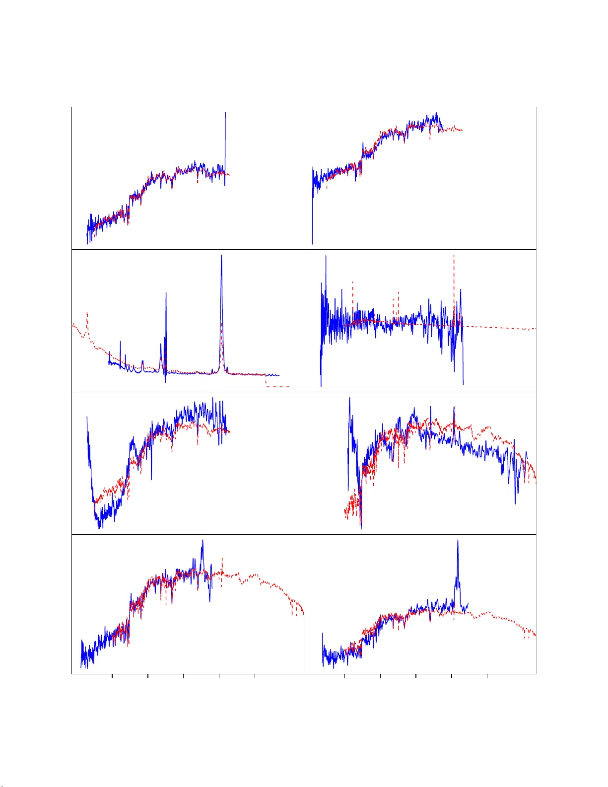
Exploiting Lo w-Dimensional Structure in Astronomical S p ectra Joseph W. Ric hards, P eter E. F reeman, Ann B. Lee, Chad M. Schafer jwrichar @stat.cmu.edu Dep a rtment of Statistics, Carne gie Mel lon Univ ersity, 5000 F orb es Avenue, Pi tts bur g h, P A 15213 ABSTRA CT Dimension-reduction tec hn iques can greatly improv e statistica l inference in astron- om y . A standard approac h is to use Principal Comp onents Analysis (PCA). In this w ork w e apply a r ec entl y-deve lop ed tec h nique, diffusion maps, to astronomical sp ectra for data parameterizati on and dimensionalit y redu cti on, and dev elop a robust, eigenmo de- based fr amew ork for regression. W e show ho w our framework pro vides a compu ta tion- ally efficien t means b y whic h to predict redshifts of galaxies, and th us could inform more exp ensiv e redsh ift estimato rs suc h as template cross-correlation. It also provides a natural means by whic h to iden tify outliers (e.g., misclassified s pectra, sp ectra with anomalous features). W e analyze 3835 S DSS s pectra and sh o w ho w our framework yields a more than 95% reduction in dimensionalit y . Finally , we sho w that the p redic- tion error of the d iffu sion map-based regression approac h is mark edly smaller than that of a similar app roac h based on P CA, clearly d emonstrating the su per iority of diffusion maps o v er PCA for this r eg ression task. Subje ct he adings: galaxies: distances and redshifts — gala xies: fundamental parameters — galaxies: statistics — metho ds: statistical — metho ds: data analysis 1. In tro duction Galaxy sp ectra are classic examples of h igh-dimensional data, with thousand s of measured fluxes providing inf o rmation ab out the physical conditions of the observed ob ject. T o mak e com- putationally efficien t inferences ab out th ese conditions, w e need to fir st r ed uce the dimensionalit y of the data space wh ile p reserving r ele v ant physica l information. W e then n ee d to find simple relationships b et ween the reduced d at a and physical p a rameters of in terest. Principal Comp onent s Analysis (PCA, or the K arh u nen-Lo ` ev e transform) is a standard metho d for the first step; its application to astronomical sp ectra is describ ed in, e.g., Boroson & Gr ee n (1992), Connolly et al. (1995), Ronen, Arag´ on-Salamanca, & Laha v (1999), F olk es et al. (1999), Madgwic k et al. (2003), Yip et al. (2004a), Yip et al. (2004b), Li et al. (2005), Zhang et al. (2006), V anden Berk et al. (2006), Rogers et al. (2007), and Re Fiorent in et al. (2007). In most cases, the authors do not pro ceed to the second step but only ascrib e p h ysical significance to the first few eigenfunctions – 2 – from PCA (su ch as the “Eigen ve ctor 1” of Boroson & Green ). Notable exceptions are Li et al., Zhang et al., and Re Fioren tin et al. Ho wev er, as we discuss in § 4, these authors com bine eigen- functions in an ad ho c mann er with no formal m et ho ds or statistical criteria for regression and risk (i.e., error) estimation. In this w ork we p resen t a unifi ed framew ork for regression an d data parameterizati on of as- tronomical sp ectra. The main idea is to describ e the imp ortan t structure of a data set in terms of its fundamental eigenmo des . Th e corresp onding eigenfunctions are u s ed b oth as co ordinates for the data an d as orthogonal basis functions for regression. W e also introd uce th e diffusion map framew ork (see, e.g., C o ifman & Lafon 2006, Lafon & Lee 2006) to astronomy , comparing and con- trasting it with PCA for regression analysis of SDSS galaxy s p ectra. PCA is a global metho d that finds linear lo w-dimensional pro jections of the d ata ; it attempts to preserv e E uclidean distances b et ween all data p oin ts and is often not robust to outliers. Th e diffusion map appr oac h, on th e other hand, is non-linear and instead retains distances that reflect the (local) connectivit y of the data. T his metho d is r ob u st to outliers and is often able to unr a v el the intrinsic geometry and the natural (non-linear) coord inate s of the data. In § 2 we describ e the diffusion map metho d for d at a parameterization. In § 3 w e introd uce th e tec h nique of adaptive r e gr ession using eigenmo des. In § 4 we demonstrate the effectiv eness of our prop osed PCA- and diffusion-map-based regression techniques for pr edict ing the redshifts of SDSS sp ectra. Our PCA- and d iffusion-map-based approac h es pro vide a fast and statistica lly rigorous means of iden tifying outliers in red shift d at a. Th e return ed em b eddings also pro vide an inf orm at iv e visualization of th e r esults. In § 5 we summarize our resu lts. 2. Diffusion Maps and Data P arameterization The v ariations in a physic al sy s te m can sometimes b e d escribed by a few parameters, while measuremen ts of the system are necessarily of ve ry high dimension; geometrically , the d ata are p oin ts in the p -dimensional space R p , with p large. In our case, a data p oint is a galaxy sp ectrum, with the dimension p giv en b y the num b er of wa v elength bins ( p & 10 3 ), and a fu ll data set could consist of hundreds of th ou s ands of sp ectra. T o mak e inference and p redictio ns tractable, on e seeks to find a simpler parameterizati on of the system. Th e most common m et ho d for dimens ion reduction and data parameterization is Principal Comp onent Analysis (PCA), where the data are pro jected on to a low er-dimensional hyper p lane. F or complex situations, ho we ve r, the assumption of linearit y may lead to sub-optimal predictions. A linear mo del pays v ery little atten tion to the natural geometry and v ariations of th e system. The top plot in Figure 1 illustrates this clearly b y sho wing a data set that f orm s a one-dimensional noisy spiral in R 2 . Ideally , w e w ould lik e to find a co ordinate system that reflects v ariations along the spir al d irect ion, which is indicated b y the dashed line. It is obvio us that any pr o jectio n of the data on to a line would b e unsatisfactory . Results of a PCA analysis of the n oisy spiral are s h o wn in the lo we r-left plot in Figure 1. – 3 – In this section, we will use diffusion maps (Coifman & Lafon, Lafon & Lee) — a n on-linea r tec h nique — to find a natural co ordinate system for the data. When searc h ing for a lo wer- dimensional description, one needs to decide what f eatures to p r eserv e and what asp ects of the data one is willing to lose. T he d iffusion map framewo rk attempts to retain the cumulativ e lo cal in teractions b et ween its data p oints, or th ei r “connectivit y” in the con text of a fictive diffusion pro cess o v er the d at a. W e demonstrate h o w this can b e a b etter m et ho d to learn the intrinsic geometry of a d at a set than b y us in g, e.g., PCA. Our str a tegy is to fi rst define a distance metric D ( x , y ) that reflects the conn ec tivit y of tw o p oin ts x and y , then find a map to a lo w er-dimensional space (i.e., a n ew data parameterization) that b est preserv es these distances. (As b efore, a “p oin t” in p -dimensional space repr esents a com- plete astronomical sp ectrum of p w a v elength bins.) T h e general idea is that we call t wo data p oints “close” if there are many short paths b et wee n x and y in a jump diffusion pro cess b et we en data p oin ts. In Figure 1, the Euclidean distance b et wee n tw o p oint s is an inappropr ia te measure of sim- ilarit y . I f, instead, one imagines a rand om w alk starting at “ x ,” and only stepping to immediately adjacen t p oin ts, it is clear that the time it w ould tak e for that wa lk to reac h “ y ” w ould r efl ec t the length along th e spiral direction. T his latter distance measure is rep resen ted by the solid path from x to y in Figure 1. W e will mak e this measure of connectivit y f orm al in w h at follo w s. The starting p oint is to construct a w eigh ted graph where the no des are th e observe d data p oin ts. The w eigh t giv en to the edge connecting x and y is w ( x , y ) = exp  − s ( x , y ) 2 ǫ  , (1) where s ( x , y ) is a locally relev ant similarity measure. F or instance, s ( x , y ) could b e chosen as the Euclidean distance b etw een x and y (denoted here k x − y k ) when x and y are v ectors. But, the c hoice of s ( x , y ) is n ot crucial, an d this gets to the heart of the app eal of this approac h: it is often simple to determine whether or n ot t wo data p oin ts are “similar”, and man y c hoices of s ( x , y ) will suffi ce for measuring this lo cal sim ilarity . The tun ing parameter ǫ is chosen small en o ugh that w ( x , y ) ≈ 0 un less x and y are similar, bu t large enough such that the constructed graph is fu lly connected. The next step is to use these w eigh ts to build a Mark o v rand om w alk on the graph. F rom no de (data p oin t) x , the p robabilit y of stepping directly to y is defined naturally as p 1 ( x , y ) = w ( x , y ) P z w ( x , z ) . (2) This probabilit y is close to zero unless x an d y are similar. Hence, in one step the random walk will mo v e only to very similar nod es (with high p robabilit y). These one-step transition probabilities are stored in the n b y n matrix P . It follo ws fr om s tand ard theory of Mark o v c hains (K emeny & Snell 1983) that, for a p ositiv e intege r t , the elemen t p t ( x , y ) of the matrix p o we r P t giv es the probability of mo vin g from x to y in t steps. In crea sing t mo ves th e random w alk forward in time, propagating the lo cal in fluence of a d ata p oint (as defined b y the k ernel w ) with its n eig hbors . – 4 – F or a fixed time (or scale) t , p t ( x , · ) is a v ector repr esen ting the distribu tio n after t steps of the random walk ov er the no des of the graph , conditional on the wal k starting at x . In what follo ws , the p oints x and y are close if the conditional distributions p t ( x , · ) and p t ( y , · ), are similar. F ormally , the diffus io n d ista nce at a scale t is d efined as D 2 t ( x , y ) = X z ( p t ( x , z ) − p t ( y , z )) 2 φ 0 ( z ) (3) where φ 0 ( · ) is the stationary distribu tio n of the r an d om walk, i.e., the long-run prop ortion of the time the wa lk sp ends at no de z . D ividing by φ 0 ( z ) serve s to redu ce the influence of no des whic h are visited with high p robabilit y regardless of the s tarting p oin t of the walk. The distance D t ( x , y ) will b e sm a ll only if x and y are connected by man y s hort paths w ith large weig hts. T his construction of a d istance measure is robust to noise and outliers b ecause it sim ultaneously accoun ts for the cum ulativ e effect of al l paths b et w een the data p oin ts. Note that the geo desic distance (the shortest path in a graph), on the other hand, often tak es shortcuts du e to noise. The final step is to find a lo w-d im en sio nal embedd ing of the data where Euclidean d is- tances reflect diffusion distances. A b iorthogo nal sp ectral d ecomp osition of the matrix P t giv es p t ( x , y ) = P j ≥ 0 λ t j ψ j ( x ) φ j ( y ), wh ere φ j , ψ j , and λ j , resp ectiv ely , rep resen t left eigen vect ors, right eigen vect ors and eigen v alues of P . It follo ws that D 2 t ( x , y ) = ∞ X j =1 λ 2 t j ( ψ j ( x ) − ψ j ( y )) 2 . (4) The pro of of Equation 4 and the details of the compu ta tion and n ormaliz ation of the eigen ve c- tors φ j and ψ j are giv en in Coifman & Lafon and Lafon & Lee. 1 By retaining the m eigenmo des corresp onding to th e m largest non trivial eigen v alues and by introd ucing th e d iffusion map Ψ t : x 7→ [ λ t 1 ψ 1 ( x ) , λ t 2 ψ 2 ( x ) , · · · , λ t m ψ m ( x )] (5) from R p to R m , w e hav e that D 2 t ( x , y ) ≃ m X j =1 λ 2 t j ( ψ j ( x ) − ψ j ( y )) 2 = || Ψ t ( x ) − Ψ t ( y ) || 2 , (6) i.e., Euclidean distance in the m -d im en sio nal em b edding defined by equation 5 appro ximates dif- fusion distance. In con trast, Euclidean distances in PC maps appro ximate the original Euclidean distances k x − y k . Again, consider the example in Figure 1. The plot on the lo w er left sho ws th a t the first diffusion map coord inate is a monotonically increasing function of the arc length of the spiral; this is n ot the case in the low er right p lot , whic h s h o ws the same relationship for th e first PC co ordinate. In deed, the relationship w ith the fi rst PC co ordinate is n ot ev en one-to-one. 1 Sample co de in Matlab and R for diffu sion maps at http://w ww.stat.cmu.ed u/~annlee/software.htm – 5 – The choice of the parameters m and t is determined by the fall-off of the eigen v alue sp ectrum as well as the pr oblem at hand (e.g., clustering, classificati on, regression, or data visualization). An ob jectiv e m easur e of p erformance should b e defined and utilized to fi nd data-drive n b est c hoices for these tun ing parameters. In this work, the fin a l goal is regression and prediction of redshift. In the next section, we s h o w how the num b er of co ordinates, m , can b e c hosen b y cross-v alidation, once one has defin ed an appr opriate statistical “risk” function. T he particular choic e of t , on the other hand , will not matter in the regression fr amew ork, as it will only repr esen t a r esca ling of th e m selected basis vect ors. 3. Adaptiv e Regression Using Orthogonal Eigenfunctions Our n ext problem is ho w to, in a statisti cally rigorous wa y , predict a fu nctio n y = r ( x ) (e.g., redshift, age, or metallic it y of galaxies) of d ata (e.g., s p ectrum x ) in v ery h ig h dimensions using a sample of known p airs ( x , y ). As b efore, imagine that our data are p oin ts in R p , but that the natural v ariations in th e system are along a low dimensional sp ac e X ⊂ R p . The set X could, for example, b e a non-linear submanif old emb edded in R p . I n our to y example in Figur e 1, X is th e one-dimensional spiral, but the data are observe d in p = 2 dimens io ns. The k ey idea is that on e ma y view the eigenfunctions from PCA or diffusion maps (a) as c o or dinates of the data p oin ts, as sh o wn in the previous section, or (b) as forming a Hilb ert orthonorm al b asis for any function (including the regression fun ction r ( x )) su pp orted on the sub set X . Rather than ap p lying an arb it rarily c h osen prediction s c heme in the computed diffu sio n or PC sp ac e (as in, e.g., Li et al., Zhang et al., and Re Fioren tin et al.), w e utilize th e latter insigh t to formulat e a general r eg ression and risk estimation framew ork. An y fun ct ion r satisfying R r ( x ) 2 dx < ∞ , where x ∈ X , can b e written as r ( x ) = ∞ X j =1 β j ψ j ( x ) , (7) where the sequen ce of fu nctio ns { ψ 1 , ψ 2 , · · · } forms an orthonormal b asis. Th e c hoice of basis functions is traditionally not adapted to the geomet ry of the data, or the set X . Standard c hoices are, for example, F ourier or wa ve let b ases for L 2 ( R p ), wh ic h are constructed as tensor p rod u cts of one-dimensional bases. Th e latter app roac h makes s ense f o r lo w dimens ions , for example for p = 2, but quic kly b ecomes intrac table as p increases (see, e.g., Bellman 1961 for the “curse of dimensionalit y”). In particular, note that if a wa ve let basis in one dimension consists of q basis functions, and hence r equires the estimation of q parameters, the naiv e tensor basis in p dimen s io ns will h a v e q p basis fun cti ons/parameters, creating an imp ossible inference problem even for mod erate p . Because this basis is not adapted to X , there is little hop e of find ing a subset of these basis functions which will do an adequate job of mo deling the r esponse. In this wo rk, we pr opose a new adaptiv e framework where the basis fun ct ions reflect the in trinsic geometry of the d ata . F u r thermore, we u se a formal statistical metho d to estimate the – 6 – risk and the optimal parameters in the mo del. First, r at her than using a generic tensor-pro duct basis for the high-dimen sio nal sp ac e R p , we construct a data-driv en b asis for th e lo wer-dimensional, p ossibly non -linear set X where the data lie. Let { ψ 1 , ψ 2 , · · · , ψ n } b e the orthogonal eige nfu nctio ns computed by PCA or diffusion m aps. Ou r regression fu nctio n estimate b r ( x ) is then give n b y b r ( x ) = m X j =1 b β j ψ j ( x ) , (8) where the different terms in the series expansion rep resen t the fun damen tal eigenmo des of the d ata, and m ≤ n is c hosen to minimize the pr edicti on risk th at we will no w define r ig orously . 3.1. Risk: Theory a nd Estimation A key asp ect of our approac h is that the c hoice of the mo dels is driv en by the minimization of a w ell-justified, ob jectiv e error criterion wh ic h comp ensates for ov erfitting. This is critical, as any basis could b e u til ized to fit the observ ed data well; this d oes not pr o vide, how eve r, an y assurance that th e mo del applies b ey ond these data. T o b egin, we establish the stand ard sto c hastic framew ork within wh ic h r egression mo dels are assessed. W e are giv en n pairs of observ ations ( X 1 , Y 1 ) , . . . , ( X n , Y n ), w ith the task of predicting the r espons e Y = r ( X ) + ǫ at a n ew d ata p oint X = x , wh ere ǫ represen ts random noise. (In § 4, the resp onse Y is the r edshift, z , and X is a complete sp ectrum.) In nonparametric regression by orthogonal fun ct ions, one assum es that r ( x ) is giv en according to equ ation (7), with its estimator giv en by equation (8), with m ≤ n where { ψ j } is a fixed basis. The primary goal is to minimize th e pr e diction risk (i.e., exp ected error), commonly quantified by the mean-squared error (MSE) R ( m ) = E [ Y − b r ( X )] 2 , (9) where the a v erage is tak en o v er all p ossible realizations of ( X , Y ), includ ing the randomness in the ev aluation p oin ts X , th e r espons es Y , and the estimates b β j . T hus, E [ · ] av erages everything that is random, including the r a nd omness in the ev aluation p oin ts X and the rand omness in the estimates b β j . This leads to protection against ov erfitting: if a basis fun cti on ψ j is unnecessarily includ ed in th e mo del, its co efficien t b β j will only add v ariabilit y or v ariance to b r ( X ) and not improv e the fit, hence increasing R ( m ). (On the other hand, as m b ecome s to o small, the estimator b ecomes increasingly biased, also increasing R ( m ).) Thus, the ideal c hoice of m is neither to o large, nor too small. In nonparametric statistic s, this is dubb ed the “bias-v ariance tradeoff” (see, e.g., W asserman 2006). A secondary goal is sp arsity ; more s pecifically , among the estimators with a small risk, w e prefer repr ese ntat ions with a smaller m . Since R ( m ) is a p opulation quant it y , one needs to app r opriate ly estimate it from the data. An estimate based on the full d at a set will un derestimat e the error and lead to a mo del w ith high bias. Here w e will use the metho d of K -fold cross-v alidation (see, e.g., W asserman ) to ac hiev e a b etter estimate of the prediction risk. The basic idea is to r an d omly sp lit th e data set into K blo c ks of – 7 – appro ximately the same size; K = 10 is a common c hoice. F or k = 1 to K , we delete blo c k k fr om the data. W e then fit the mo del to the remaining K − 1 blo c ks and compute the observe d squared error b R ( − k ) ( m ) on the k th blo c k wh ich was n ot included in the fit. The CV estimate of the risk is defined as b R C V ( m ) = 1 K P K k =1 b R ( − k ) ( m ). It can b e s ho wn that this quantit y is an app ro ximately unbiase d estimate of the true error R ( m ). Thus, we c ho ose th e mo del parameters that minimize the CV estimate b R C V ( m ) of the r isk, i.e., we tak e m opt = arg min b R C V ( m ). Finally , w e note that the id eas of C V introd uced here generalize to cases where the mo del parameters are of higher dimension. F or example, in the diffusion m ap case, the r isk is m inimized o v er b oth the bandwid th ǫ and the n um b er of eigenfunctions m . T he CV estimate of the risk is implemen ted in the same fashion, b ut the searc h sp ac e for fin ding the minimum is larger. In what follo ws , the notation will mak e it clear wh ich mo del parameters w e are minimizing o ver b y writing, for example, R ( ǫ, m ). T o s ummarize, our claim is that the prop osed regression f ramew ork will lead to efficient infer- ence in h ig h dimensions, as we are effectiv ely p erforming r eg ression in a lo wer-dimensional space X that captures the natural v ariations of the data, where the optimal dimens ionalit y is c hosen to minimize pr edict ion risk in our regression task. Finally , th e u s e of eigenfunctions in b oth the data p aramet erization and in the r eg ression formulat ion pr o vides an elega nt, unifying framew ork for analysis and prediction. 4. Redshift Prediction Using SDSS Sp ectra W e apply the formalism p resen ted in §§ 2-3 to the pr oblem of predicting redshifts f or a sample of SDSS sp ectra. Physica lly similar ob j ects residing at similar redshifts will ha v e similar con tin uum shap es as well as absorption lin es o ccurring at similar w a v elengths. Hence the Euclidean distances b et ween their sp ectra will b e small. The prop osed r egression fr amew ork with diffus ion map or P C co o rd in at es pr o vides a natural means by which to predict redshifts. F ur thermore, it is computa- tionally efficien t, making its use app ropriate for large databases su c h as the S DSS; one can use th ese predictions to inform more compu ta tionally exp ensive tec h n iques by narro wing do wn the relev an t parameter space (e.g., the redshift range or the set of templates in cross-correlation tec h n iques). Adaptiv e regression also p r o vides a usefu l tool for quic kly identifying anomalous d ata p oin ts (e.g., ob jects misclassified as galaxie s), galaxies th at ha v e relativ ely rare features of in terest, and galaxies whose SDSS redsh ift estimates may b e incorrect. 4.1. Data Preparation Our initial data sample consists of sp ectra that are classified as galaxies from ten arb itrarily c hosen sp ectroscopic plate s of SDSS DR6 (02 66 − 0274 inclusive, and 0286; Adelman-McCarthy et al. 2008). W e r emo v e s pectra from this sample b y applyin g three cuts. T h e firs t is motiv ated by ap er- – 8 – ture considerations: w e analyze on ly those s p ectra with S DS S redshift estimates z SDSS ≥ 0.05. T o include sp ectra with z SDSS < 0 . 05 w ould b e to add an extra s o ur ce of v ariation that w ould adv ersely imp ac t regression analysis. Th e second cut is based on bin flags. T o av oid calibration issues observed at b oth the low and high wa v elength ends , w e remov e the first 100 and last 250 w a v elength bins from eac h sp ectrum; then w e d et ermine what prop ortion of the remaining 3500 bins are flagged as bad. If this prop ortion exceeds 10%, we remo v e the sp ectrum from th e sample; if n o t, we r eta in the red u ced s pectrum for fur ther analysis. W e pr o vide details on the third cut b elo w. The application of th ese cuts red u ces our sample size from 5057 to 3835 gala xies. W e fur ther pro cess eac h sp ectrum in our samp le as follo ws. • W e replace the fl ux v alues in the vicinit y of prominent atmosph eric lines at 5577 ˚ A, 6300 ˚ A, and 6363 ˚ A with the sample mean of the nine closest bins on either side of eac h line. T he flux errors are estimated by av eraging (in quadrature) the standard errors of the flu xes for these bins. • W e similarly replace the flu x v alues in eac h b in flagged b y SDSS as part of an emission lin e, with flux and flux error estimates b ased up on the closest 50 bins on either side of the line. (Within this group of 100 bins, w e d o not include those that are themselv es fl ag ged as emission lines.) W e do this b ecause highly v ariable emission line stren g ths can s tr o ngly b ia s distance calculatio ns. • Last, after replacing flux v alues as necessary , w e normalize eac h sp ectrum to sum to 1 to mitigate v ariation due to differences in luminosit y b et wee n similar galaxie s at similar r edshifts. In its d ata reduction pip eline, SDSS estimates sp ectroscopic redsh if ts, z SDSS , standard errors, σ z SDSS , and “confidence level s,” CL, the latter of which are functions of the strengths of obs erv ed lines (and th u s should not b e in terpreted probabilistically). 2 Lac k in g kno wledge of the true redsh ifts in our s ample, we use z SDSS and σ z SDSS to fit our regression mod el. Sin ce p o orly estimated r edshifts can bias the mo del, we d ivide our data sample into t wo groups, fitting with only those 279 3 gala xies with CL > 0.99. W e then use the fitted mo del to p redict redsh ifts for the other 1042 galaxies. (It is here that w e m ak e our third data cut: to a void issues of extrap ol ation, we r emo v ed 19 of 1061 sp ectra with CL ≤ 0.99 whose S DS S reds hift estimate s lie outsid e the range of ou r training set, i.e. th ose with z SDSS > 0 . 50.) As s ho wn in Figure 2, the distributions of r edshifts in our high- and lo w -CL samples are similar, implying that p redicte d redsh ifts f o r lo w-CL galaxies from the mo del built on high-CL galaxies should not b e systematically b iased. 2 See http://www.sd ss.org/dr6/algorit hms/redshift type.html . – 9 – 4.2. Analysis In this section, w e p erform b oth PCA and d iffusion m ap for our sample and predict redshift using the regression mo del introduced in § 3. W e provide details on the PCA algorithm in App end ix A. In the diffus ion map analysis, we b egin by calculating Eu clidea n d ista nces b etw een s pectra s ( x , y ) = s X k ( f x ,k − f y ,k ) 2 , (10) where f x ,k and f y ,k are the normalized flu xes in bin k of sp ectra x and y , resp ectiv ely . W e use these distances and a c hosen v alue of ǫ to constru ct b oth the weig hts for the graph (see equ ation 1) and the transition matrix P (see equation 2), f r om which eigenmod es are generated. Belo w w e discus s ho w we select the optimal v alue of ǫ . As stated in § 2, the v alue of the parameter t (see equation 5) is un imp o rtant in the con text of regression, as an y c hange in t w ould b e met w it h a corresp onding rescaling of the coefficients b β j in the r egression mo del, su c h that predictions are un changed. In Figure 3 we plot the embed ding of th e 2793 galaxie s with CL > 0.99 in th e fir s t thr ee P C and d iffusion map co ordinates (e.g., λ t i ψ i ( · ) in equation 5). W e obs erv e that the structure of eac h of these reparameterizations of the original d ata corresp onds in a simple w a y to log 10 (1 + z SDSS ). These emb eddings are a useful wa y to visualize the data and to qualitativ ely iden tify subgroup s of data and p eculiar data p oin ts. In the next stage of analysis we use the computed eigenfunctions to pr edict z for our samp le of 3835 galaxies. W e regress z SDSS up on the diffu s io n m ap (and PC) eigenmodes (cf. equation 8, where b r repr esen ts our redshift estimates), weigh ting eac h d at a p oin t by the inv erse v ariance of its z SDSS , 1/ σ 2 z SDSS , to accoun t for the uncertaint ies in z SDSS measuremen ts. W e rep eat this step for a sequence of m (and ǫ ) v alues, determinin g th e optimal v alues of eac h by min imizi ng the p redictio n risk R ( ǫ, m ), estimated via ten-fold cross-v alidation (see equation 9 and sub sequen t discussion). It is in th is regression step that w e clearly observe the adv ant age of using diffusion m a ps o v er pr incipal comp onen ts. In Figure 4 we sh ow that diffusion map achiev es significantly low er CV p redictio n risk f or most c hoices of mo del size m and obtains a muc h lo we r m inim u m b R CV , i.e., th e optimal lo w -dimensional diffusion map representa tion of our data captures the trend in z b etter than the PC representa tion. Note that the trend in b R CV for b oth PC and d iffu sion map basis fu nctio ns is to decrease with increasing mo del size for small mo dels and to increase with increasing mo del size for larger mo dels. Th is is the “bias-v ariance tradeoff” that was r eferred to in § 3.1: as the size (complexit y) of our mo del increases, the bias of the m o del decreases while the v ariance of the m odel increases. Pr edict ion risk is th e sum of the squared bias and v ariance of a mo del, explaining the b eha v ior observ ed in Figure 4: for s mall mo dels, increasing mo del size leads to decrease in b ia s that o v erwhelms increase in v ariance while for large mo dels, in crea se in mo del size pro duces minimal decrease in bias and relativ ely large increase in v ariance. In T able 1, we sho w the parameters for the optimal (minimal b R CV ) diffusion map and PC – 10 – regression mo dels. Note that since our original data w ere in 3500 dimensions, our optimal diffusion map mo del ac hiev es a 96.4% r eduction in dimensionalit y . If we were to choose an arbitrary small mo del size as is often done in th e literature, our prediction risk estimates w ould b e terrible. F or example, for mo del sizes m = 10 and 20, th e CV prediction risks for regression on PC b asis functions are 0.305 and 0.209 , resp ectiv ely (compared to optimal v alue 0.193), wh ile regression on diffu s io n map b asis functions yields b R CV of 0.295 and 0.191 , resp ectiv ely (compared to optimal v alue 0.134). The choice of ǫ in th e diffusion map mo del also h as a significan t imp a ct on results. F or v alues of ǫ that are to o sm all, CV r isks are extremely large b ecause the data p oin ts are no longer connecte d in the diffusion pro cess and consequently large outliers occur in the d iffusion map parameterization. Lik ewise, large v alues of ǫ yield large pr ed ic tion r isks due to the large w eigh ts giv en to connections b et ween dissimilar data p oin ts. In Figure 5 w e plot pr ed ic tions and prediction inte rv als for all galaxies in our sample using our optimal diffusion map mo del. (See App endix B for a discussion of prediction in terv als.) Most of our predictions are in close corresp ondence with the S DSS estimates. W e obser ve p ositiv e correlation in the amoun t of disparit y b et ween our redshift estimat es and SDSS estimates v ersus 1-CL (Figure 6) meaning that galaxie s for wh ic h our estimates disagree with SDSS estimates are more lik ely to b e galaxies w ith lo w CL. There are 54 outliers at the 4 σ lev el. Visu al insp ection of their sp ectra indicates that 39 app ear to fit the template assigned b y SDSS. Of these, 27 are well- describ ed by the LRG template. In Figure 7 w e show that most of the outliers that are well-fit by their S DSS templates are fain t ob jects. A plausible exp la nation for their classificatio n as outliers is lo w S /N in their measur ed sp ectra. F ain t galaxies with strong emission lines will generally ha ve accurate SDSS redshifts but can b e outliers in th e diffusion map b ecause noisy sp ectra indu ce higher Euclidean d ista nces. In a future pap er w e w ill introd uce a metho d to acco unt for errors in the original measured data th a t corrects b oth for err ors in Euclidean d istance computations and r andom errors in the diffusion map co o rd in at es. The 15 other outliers sho w interesting and/or anomalous features. F our sp ectra app ear to b e LR G t yp e galaxies with abnorm al emission and /or absorption f ea tures, of whic h at least t w o are lik ely att ribu ted to calibration err ors (see Figure 8a,b). On e sp ect rum is clea rly a QSO (Figure 8c), one sho ws only sky sub tract ion resid uals (Figure 8d), and t wo others are ob vious mismatc hes to their SDSS templates due to absorption lines w hose depths do n ot matc h their assigned template. F our outliers h a v e abnormal bum ps (p ossible contin uu m jumps d ue to instrum ental artifacts, s ee Figure 8e,f ) that app ear lik e w ide emission f ea tures. One outlying galaxy has a sp ectrum that lo oks lik e a late-t yp e galaxy with n o emission lines, meaning it is lik ely a K+A p ost-starburst galaxy . Another outlier h as an anomalous emission feature around 6000 ˚ A in rest frame (Figure 8g). This is a p ossible lens galaxy , but w as not selected b y the Sloan Lens A CS Survey (SLA CS; Bolton et al.) b ecause the feature in question o cc urs in close p r o ximit y to str o ng sky lines at 8800 ˚ A . The fi nal outlier has a strong, wide emission feature in the vicinit y of H α but has no emission lines an ywhere else in the SDSS sp ectrum (Figure 8h). None of the outlying sp ectra sho w conclusiv e evidence of a – 11 – wrong S DSS redshift measurement (except for the afore-mentio ned sky sp ectrum, whic h w e detect as a 30 σ outlier). 4.3. Comparison With O ther Metho ds As discussed in § 1, many authors hav e applied PCA to gala xy sp ectra in an attempt to reduce the dimens ionalit y of the data space, but few attempt to find simple relationships b et ween th e re- duced data and the physica l parameters of interest; these exceptions in clude Li et al. , Zhang et al., and Re Fiorentin et al. In all three cases, the authors use P CA to estimate stellar and/or galactic parameters that are traditionally estimated by lab oriously measur ing equiv alen t width s and flu x es of individual lines, ju st as we hav e u sed diffusion map eigenfunctions to estimate redshift, a physi- cal parameter usually estimated through computationally intensiv e cross-correlation metho ds. W e stress three adv an tages of our appr oa c h o ver those emplo yed by the ab o ve authors: 1) W e ac hiev e m uc h low er prediction error u sing diffusion map co ordinates as compared to PCA, 2) we h a ve an ob jectiv e w a y of selecting the p aramet ers of the mo del, and 3) w e u se a theoretically well-mot iv ated regression mo del w hic h tak es s ta tistical v ariations of the data into accoun t and which unifies th e data parameterization and regression algorithms. The aim of Li et al. is to estimate, e.g., the v elo cit y disp ersion and r eddening of a set of appro ximately 1500 galaxies observ ed b y SDSS. Th ey use PC A in tw o su cc essiv e applications. They first apply PCA to the ST ELIB library to reduce 204 stellar sp ectra to 24 stellar eigensp ectra. Th ese in turn are fit to SDSS DR1 sp ectra to create a library of 1016 galacti c sp ectra, whic h are red uced to nine galactic eigensp ectra. The authors then regress observed equ iv alen t widths (EW) and fluxes of H α up on these nine eigensp ectra. They determine the num b er of eigensp ectra to retain b y estimating noise v ariance in the s te llar case and by using th e F test to compute the s ig nificance of eac h additional eigensp ectrum in sp ectral r ec onstru ction in the galactic case. The latter criterion ho w ev er is not well -suited to the task of parameter estimation b ecause the appropriate num b er of comp onen ts in the regression mo del dep ends on the complexit y of the dep endence of those parameters as a function of the b asis elements, not on the complexit y of the original sp ectra. F or example, the dep endence of th e EW of H α on the PC b asis functions ma y b e a simple, smo oth function while the fl ux dep endence ma y b e complex, bumpy r ela tionship. In this case, the optimal regression mo del to p redict EW w ould require fewer b asis functions than the optimal mo del for H α flux p r edicti on. Minimizing CV risk would lead us to choose the correct num b er of b a sis functions for eac h task, wh ile the metho d of Li et al. would force us to use th e same (inapp r opriate ) size for eac h mo del. Zhang et al. attempt to predict stellar parameters by regressing on PC co efficien ts using a k ernel regression mo del with a v ariable w indo w width. In their pap er, they do not sp ecify ho w to select the win do w width (they in tro duce an arbitrary parameter λ ) or ho w to c ho ose the correct n umb er of PC b asis fu nctions (they use 3). Th eir choice of a small m odel size is like ly d ue to the computational and statistical difficulties that c haracterize k ernel regression in high dimensions – 12 – (W asserman 2006). Re Fioren tin et al. attempt to estimate stellar atmospheric parameters (effectiv e temp erature, surface gra vit y , and metallicit y) f r om SDSS/SEGUE sp ectra. T hey use PCA for dimension reduc- tion, b ut s et m to an arbitrary v alue (e.g., 50). T hey th en use an iterativ e, n on-linea r regression mo del (utilizing the h yp erb olic tangent function; see Bailer-Jones 2000), with an error fun ct ion based on the residu al sum -o f-squares p lus a regularization term (see their equation 2). Again, the c hoice of the regularization parameter is not justified . W e fi nd that when applied to the same data set of galaxy sp ectra, their mo del do es not ac hiev e low er CV risk than our mo del for differen t c hoices of regularizatio n parameter and mo del size. 5. Summary The p urp ose of th is pap er is t w o-fold. First, w e in tro duce the diffusion map metho d for data parametrization and d imensionalit y redu ctio n. W e show th at f or the t yp es of high-dimensional and complex data sets often analyze d in the astronom y , d iffusion map can yield far sup erior resu lts than commonly-used metho ds suc h as PCA. Moreo v er, the simple, in tu iti ve formulation of diffusion map as a metho d that preserves the lo cal interacti ons of a high-dimensional d at a set makes the tec h nique easily accessible to scien tists th at are n ot well -v ersed in statistics or mac hine learning. Second, w e pr esent a fast and p ow erful eigenmo de-based framew ork f or estimating physical parameters in databases of high-dimensional astronomica l data. In most astroph ysical applications, PCA is used as a data-explorativ e to ol f o r dimensionalit y reduction, with no formal m et ho ds and statistica l criteria for r eg ression, r isk estimation and selection of relev an t eigen v ectors. Here we prop ose a statistically rigorous, u nified fr amew ork for regression and d ata p a rameterization. Our prop osed regression mo del combines basis fun ct ions in a simp le and statistically-motiv ated manner while ou r clear ob j ec tiv e of risk minimization d riv es the estimatio n of the mo del parameters. Again, the simplicit y of the prop osed metho d w ill mak e it app ealing to th e non-sp ecialist. W e apply the pr oposed metho dology to pr edict redsh ift for a s amp le of SDSS galaxy s p ectra, comparing the use of the p rop ose d regression mo del with PCA basis functions versus d iffu sion map basis functions. W e find that the prediction error for the diffu sion-map-based appr oa c h is mark edly smaller than that of a similar framew ork based on PCA. Our tec h n iques are also more robust than commonly used template matc hing metho ds b ecause they consider th e stru cture of the entire high-dimensional data set when r eparamet rizing the data. Statistical inferences are based on th is learned structur e, instead of consid ering eac h data p oint separately in an ob ject-b y- ob ject matc hing algorithm as is current ly used b y SDSS and commonly emplo ye d th roughout the astronom y literature. W ork in progress extends our app roac h to photometric redshift estimation and to the estimation of the int rins ic parameters (e.g., mean metalliciti es and ages) of galaxies. The authors would lik e to thank Jeff Newman for helpful con ve rsations. This w ork w as sup- – 13 – p orted by NS F gran t #0707059 and ONR grant N00014-08- 1-0673. A. Principal C omponents Analysis W e fi rst cen ter our data (the normalized sp ectra with p wa vel ength b ins) so that 1 n P n i =1 x i = 0. The cen tered obser v ations x 1 , x 2 , . . . x n ∈ R p are then stac ke d in to the ro ws of an n × p matrix X . Note th a t the sample co v ariance matrix of x is giv en by th e p × p matrix S = 1 n X T X . In Principal C omponent Analysis (PCA), one compu tes the eigen ve ctors of the co v ariance matrix that corr esp ond to the m < p largest eigen v alues; den ote these vect ors by v 1 , . . . , v m ∈ R p . In a PC map , the pro jections of the data on to these vec tors are then used as new co ordinates; i.e. th e PC em b edding of data p oint x i is giv en b y the map x i 7→ Ψ PCA ( x i ) = ( x i · v 1 , . . . , x i · v m ) . These pro jections are sometimes referr ed to as the p rincipal comp onen ts of X . Algorithmically , the PC emb edding is easy to compute usin g a sin gu lar v alue decomp osit ion (SVD) of X : X = UDV T . Here U is an n × p orthogonal matrix, V is a p × p orthogonal matrix (where the columns are eigen vect ors v 1 , . . . , v p of S ), and D is a p × p diagonal matrix with d ia gonal elemen ts d 1 ≥ d 2 . . . ≥ d p ≥ 0 kn o wn as the singular v alues of X . Since XV = UD , the PC em b edding of the i :th d at a p oin t in m dimens ions is giv en by the fi rst m element s of the i :th r ow of UD . B. Prediction In terv als for Sp ectrosc opic Redshift Estimat e s In an y one fold of a ten-fold regression analysis, we fit to 90% of the data, generating predictions and p redictio n inte rv als for the 10% of the data withheld from the an alysis. A pred ic tion in terv al is not a confidence in terv al; the form er denotes a plausible r ange of v alues for a single ob s erv atio n, whereas the latte r denotes a plausible range of v alues for a parameter of the p robabilit y d istribution function from wh ic h that single observ ation is sampled (e.g., the mean). Let X and ˜ X represent the matrices of indep endent v ariables includ ed in, and withh eld from, regression analysis, r espectiv ely . F or instance, ˜ X =    ψ 1 ( x 1 ) · · · · · · ψ m ( x 1 ) . . . . . . . . . . . . ψ 1 ( x n ) · · · · · · ψ m ( x n )    , where n is the num b er of withheld data and m the num b er of assum ed basis functions. (Here, w e lea ve out factors of λ t j , w hic h are s u bsumed into the estimated regression co effici ents b β j .) The – 14 – v ector of redshift predictions for the w it hh el d d at a is thus b z = ˜ X b β , where b β is estimated from X while the vec tor of half-prediction interv als is giv en b y t α/ 2 ,N − n − 2 b σ r ˜ X ( X T X ) − 1 ˜ X T + 1 + 1 N − n , (B1) where b σ is the estimated s tand ard deviation of th e r andom noise ǫ in the relationship Y = r ( X ) + ǫ , estimated from the residu al s of the regression of Y up on X , t α/ 2 ,N − n − 2 is the critical t-v alue for a t wo-sided 100(1- α )% p r edicti on inte rv al, and N is the total num b er of data p oin ts. Equation (B1) is a multi-dimensional generalizatio n of, e.g., equ ation (2.26) of W eisb erg (2005), taking into accoun t that the m ea n of ψ ( x ) is zero. – 15 – REFERENCES Adelman-McCarth y , J. K., et al. 2008, ApJS , 175, 297 Bailer-Jones, C. A. L. 2000, ˚ a, 357, 197 Bellman, R. E. 1961, Adaptiv e Control Pr ocesses (Prin ce ton Un iv. Press) Boroson, T. A., & Gr ee n, R. F. 1992, ApJ S, 80, 109 Bolton, A. S ., et al. 2006, ApJ, 638, 703 Coifman, R. R., & Lafon, S. 2006, Ap pl. Compu t. Harmon. Anal., 21, 5 Connolly , A. J., Szala y , A. S., Bershady , M. A., Kinn ey , A. L., & C alzetti, D. 1995, AJ, 110, 1071 F olk es, S., et al. 1999, MNRAS, 308, 459 Kemen y , J. G., & Snell, J. L. 1983, Finite Mark o v Chains (Springer). Lafon, S., & L ee , A. 2006, IEEE T rans. Patte rn Anal. and Mach. Inte l., 28, 1393 Li, C., W ang, T.-G., Zhou, H.-Y., Dong, X.-B., & C heng, F.-Z. 2005, AJ, 129, 669 Madgwic k, D. S ., et al. 2003, ApJ, 599, 997 Re Fioren tin, P ., et al. 2007, A&A, 467, 1373 Rogers, B., F erreras, I., Laha v, O., Bernard i, M., Ka vira j , S., & Yi, S. K. 2007, MNRAS, 382, 750 Ronen, S., Arag´ on-Salamanca, A., & Laha v, O. 1999, MNRAS, 303, 284 V anden Berk, D. E., et al. 2006 , AJ, 131, 84 W asserman, L. W. 2006, All of Nonparametric Statistics (New Y ork:Sprin g er) W eisb erg, S. 2005, Ap plied Linear Regression (Hob ok en:Wiley) Yip, C. W., et al. 2004, AJ, 128, 585 Yip, C. W., et al. 2004, AJ, 128, 2603 Zhang, J., W u, F., Luo, A., & Zhao, Y. 2006, ChJ AA, 30, 176 This p reprin t w as prepared with t he AAS L A T E X macros v5.2. – 16 – −2.5 −2 −1.5 −1 −0.5 0 0.5 1 1.5 2 −1.5 −1 −0.5 0 0.5 1 1.5 2 x y 0 0.1 0.2 0.3 0.4 0.5 0.6 0.7 0.8 0.9 1 0 0.1 0.2 0.3 0.4 0.5 0.6 0.7 0.8 0.9 1 Normalized Diffusion Map coordinate Normalized arclength along spiral 0 0.1 0.2 0.3 0.4 0.5 0.6 0.7 0.8 0.9 1 0 0.1 0.2 0.3 0.4 0.5 0.6 0.7 0.8 0.9 1 Normalized PC coordinate Normalized arclength along spiral Fig. 1.— An example of a one-dimensional manifold (dash ed lin e) with Gaussian noise em b edded in tw o or higher dimensions. The p ath (solid line) from x to y reflects th e natural geometry of the data set whic h is captured by the diffusion d ista nce b et wee n x and y . The plot on th e lo wer left sho ws that the fi rst diffu sion map co ordinate is a monotonically increasing function of the arc length of th e sp ir al ; th is is n ot the case in the lo wer right p lot , whic h sh o ws the s ame relationship for the fi r st PC co ordinate. – 17 – Number of Galaxies 0.0 0.1 0.2 0.3 0.4 0.5 0 200 400 600 800 CL > 0.99 Redshift Number of Galaxies 0.0 0.1 0.2 0.3 0.4 0.5 0 100 200 300 CL ≤ 0.99 Fig. 2.— Distrib utions of SDSS r edshift estimates in our high-CL (top) and lo w-CL (b ottom) samples. W e train our regression mo del u sing the 2793 high-CL galaxi es only , then apply those predictions to the 1042 low-CL galaxies. – 18 – −0.03 −0.02 −0.01 0 0.01 −0.02 0 0.02 0.04 0.06 −0.03 −0.02 −0.01 0 0.01 0.02 0.03 0.04 PC1 PC Map PC2 PC3 0.04 0.06 0.08 0.1 0.12 0.14 0.16 −6 −4 −2 0 2 4 6 x 10 −7 −25 −20 −15 −10 −5 0 5 x 10 −12 −15 −10 −5 0 5 x 10 −11 λ 1 t ψ 1 Diffusion Map λ 2 t ψ 2 λ 3 t ψ 3 0.04 0.06 0.08 0.1 0.12 0.14 0.16 Fig. 3.— Emb edding of our sample of 2793 SDSS galaxy sp ectra with SDSS z CL > 0 . 99 with the first 3 PC and the fi rst 3 diffusion m ap co ordinates, resp ectiv ely . T he co lor co des for log 10 (1 + z SDSS ) v alues. Both maps sho w a clear corresp onden ce with redshift. – 19 – 0 50 100 200 300 0.15 0.20 0.25 0.30 # of basis functions CV Prediction Risk Diffusion Map PCA Fig. 4.— Risk estimates ( b R C V ) for regression of z on diffusion map coord in at es and PCs . Diffusion map attains a lo w er risk for almost ev ery n umber of co ordinates in th e regression. I t also ac hieves a lo we r minimum risk as indicated b y T able 1. R isk estimates are based on 50 rep etitions of 10-fold CV. Th ic k lines r epresen t mean risk at that mo del size and thin dotted lines are +/- 1 standard deviation bands. – 20 – 0.00 0.10 0.20 0.00 0.10 0.20 CL < 0.99 SDSS log(1+z) predicted log(1+z) 0.95 0.99 SDSS log(1+z) predicted log(1+z) 2793 galaxies Fig. 5.— Reds hift pr ed ic tions u sing diffusion map co o rd in at es f or galaxies with SDSS C L ≤ 0.99 (top) and CL > 0.99 (b ottom), eac h plotted against z SDSS . Error bars rep r esen t 95% pr edicti on in terv als. Note that CL ≤ 0.99 red shift predictions are b ase d on the m o del trained on CL > 0.99 galaxies while CL > 0.99 p redictio ns are from 10-fo ld CV on CL > 0.99 galaxies. F or m ost galaxies, our predictions are in close corresp ondence with SDS S estimates. – 21 – −5 −4 −3 −2 −1 0 0 2 4 6 8 10 SDSS log(1−CL) # sigma discrepancy 5 sigma 3 sigma 1 sigma Fig. 6.— Discrepancy b et we en our pr edict ed red shift v alues and z SDSS estimates ve rsu s log (1-CL). There is a correlation of 0.392 b et we en the amoun t of discrepancy and 1-CL, meaning that gal axies for which there are large differences b et ween the tw o redshift estimate s tend to b e ob jects whose SDSS r ed shift confidences are lo w. Horizon tal lines denote 1, 3, and 5 σ disparities. Small random p erturbations h a v e b een add ed to dup lica te log(1-CL) v alues to visualize galaxies with the same CL. Galaxies with a CL of 1.00 are assigned mean log(1-CL) of -4. – 22 – 3.0 3.5 4.0 4.5 5.0 5.5 0 2 4 6 8 10 log(flux) (log(10^(−17) erg/cm/s^2/Ang)) # sigma discrepancy match LRG template match galaxy template match other template Fig. 7.— Discrepancy b et wee n our p redicted reds h ift v alues and z SDSS v ersus log(flux) of the original sp ectra. Th er e is a correlation of -0.327 b et w een the amount of discrepancy and galaxy brigh tness. Galaxies can b e detected as outliers ev en if they matc h w ell to their SDSS template (in color). L ow S/N can cause normal galaxies with correct S DSS r ed shifts to b e lab eled as outliers. W e also d ete ct sev eral physica lly in teresting ob jects as outliers (see Figure 8). – 23 – mjd = 51630, plate = 266, fiber = 10 , objid = 756 1 1 206 260 (a) mjd = 51883, plate = 271, fiber = 276, objid = 752 1 3 70 47 (b) mjd = 51910, plate = 269, fiber = 276, objid = 752 1 3 48 52 (c) mjd = 51913, plate = 274, fiber = 530, objid = 756 1 6 296 724 (d) mjd = 51630, plate = 266, fiber = 636, objid = 756 1 4 210 499 (e) mjd = 51633, plate = 268, fiber = 637, objid = 752 1 4 45 183 (f) mjd = 51909, plate = 270, fiber = 630, objid = 752 1 5 69 253 (g) 3500 4500 5500 6500 7500 Wavelength ( A ° ) mjd = 51957, plate = 273, fiber = 394, objid = 752 1 4 92 271 (h) 3500 4500 5500 6500 7500 Wavelength ( A ° ) Fig. 8.— Eigh t selected outliers w ith anomalous features. Eac h sp ectrum (solid blue) is plotted along with its SDS S template matc h (dashed red). Sp ectra are scaled to ha v e the same sum of squared (smo othed) fluxes o v er the same range of wa vel engths. F or a thorough discussion of th ese outliers see § 4.2 – 24 – T able 1. Parame ters of Optimal Regression on log 10 (1 + z SDSS ) Num b er of Outliers ǫ opt m opt b R C V ( ǫ opt , m opt ) a 3 σ 4 σ 5 σ Diffusion Map .0005 127 0.1341 115 54 20 PC – 88 0.1931 109 55 20 a Prediction risk estimated via cross-v alidation; see equation (8) and subsequent discussion.