Vector Diffusion Maps and the Connection Laplacian

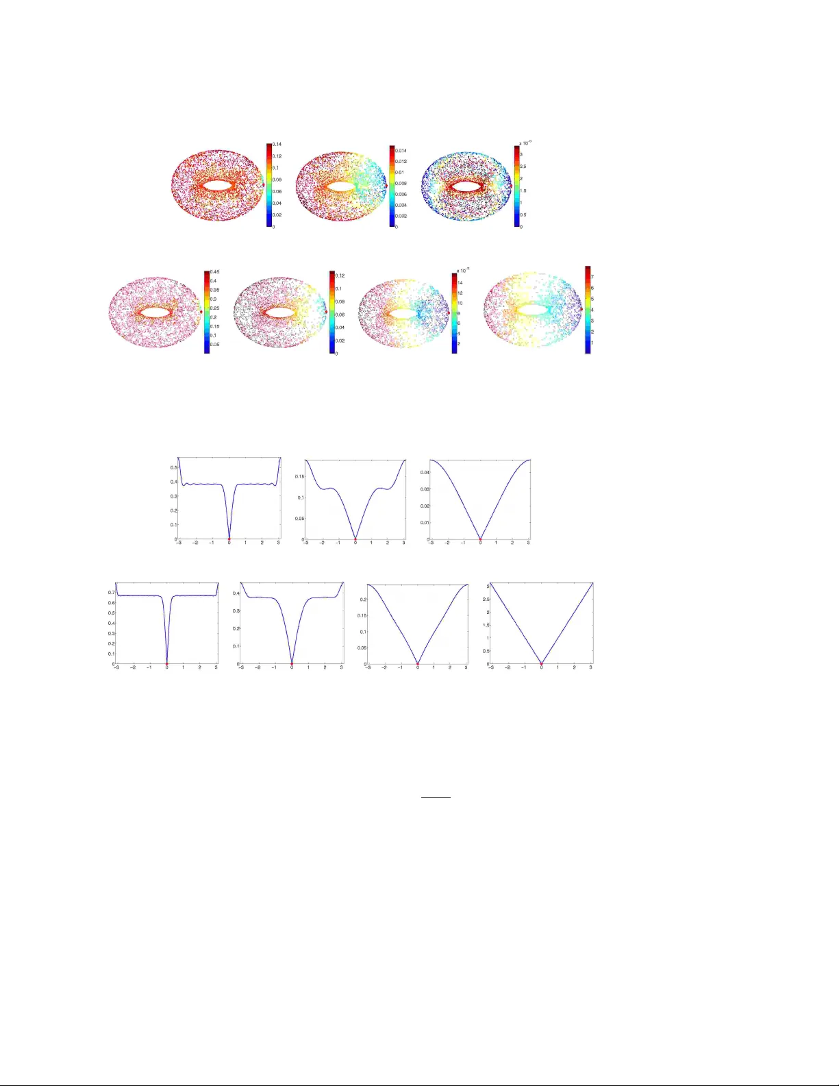
VECTOR DIFFUSION MAPS AND THE CONNECTION LAPLA CIAN A. SINGER ∗ AND H.-T. WU † De dic ate d to the Memory of Partha Niyo gi Abstract. W e in tro duce ve ctor diﬀusion maps (VDM), a new mathematical framew ork for orga- nizing and analyzing massiv e high dimensional data sets, images and shapes. VDM is a mathematical and algorithmic generalization of diﬀusion maps and other non-linear dimensionality reduction meth- ods, such as LLE, ISOMAP and Laplacian eigenmaps. While existing metho ds are either directly or indirectly related to the heat kernel for functions o ver the data, VDM is based on the heat kernel for vector ﬁelds. VDM provides to ols for organizing complex data sets, embedding them in a low di- mensional space, and interpolating and regressing vector ﬁelds ov er the data. In particular, it equips the data with a metric, which we refer to as the ve ctor diﬀusion distanc e . In the manifold learning setup, where the data set is distributed on (or near) a low dimensional manifold M d embedded in R p , we prov e the relation b etw een VDM and the connection-Laplacian op erator for vector ﬁelds over the manifold. Key words. Dimensionality reduction, vector ﬁelds, heat kernel, parallel transp ort, local prin- cipal component analysis, alignment. 1. In tro duction. A popular w ay to describe the aﬃnities betw een data points is using a weigh ted graph, whose vertices corresp ond to the data p oints, edges that con- nect data p oints with large enough aﬃnities and weigh ts that quantify the aﬃnities. In the past decade we ha ve b een witnessed to the emergence of non-linear dimension- alit y reduction metho ds, such as lo cally linear embedding (LLE) [33], ISOMAP [39], Hessian LLE [12], Laplacian eigenmaps [2] and diﬀusion maps [9]. These metho ds use the lo cal aﬃnities in the weigh ted graph to learn its global features. They provide in v aluable to ols for organizing complex netw orks and data sets, embedding them in a lo w dimensional space, and studying and regressing functions o ver graphs. Inspired b y recen t developmen ts in the mathematical theory of cry o-electron microscopy [36, 18] and synchronization [34, 10], in this pap er we demonstrate that in many applications, the representation of the data set can b e v astly improv ed by attac hing to every edge of the graph not only a weigh t but also a linear orthogonal transformation (see Figure 1.1). Consider, for example, a data set of images, or small patches extracted from images (see, e.g., [27, 8]). While weigh ts are usually deriv ed from the pairwise com- parison of the images in their original representation, we instead asso ciate the weigh t w ij to the similarit y b etw een image i and image j when they are optimally rotation- ally aligned. The dissimilarity b et ween images when they are optimally rotationally aligned is sometimes called the rotationally inv arian t distance [31]. W e further deﬁne the linear transformation O ij as the 2 × 2 orthogonal transformation that registers the t wo images (see Figure 1.2). Similarly , for data sets consisting of three-dimensional shap es, O ij enco des the optimal 3 × 3 orthogonal registration transformation. In the case of manifold learning, the linear transformations can b e constructed using local principal comp onent analysis (PCA) and alignment, as discussed in Section 2. While diﬀusion maps and other non-linear dimensionality reduction metho ds are either directly or indirectly related to the heat kernel for functions ov er the data, ∗ Department of Mathematics and P ACM, Princeton Universit y , Fine Hall, W ashington Road, Princeton NJ 08544-1000 USA, email: amits@math.princeton.edu † Department of Mathematics, Princeton Univ ersity , Fine Hall, W ashington Road, Princeton NJ 08544-1000 USA, email: hauwu@math.princeton.edu 1 Fig. 1.1 . In VDM, the r elationships b etween data p oints are repr esented as a weighte d gr aph, wher e the weights w ij ar e ac comp anie d by line ar orthogonal tr ansformations O ij . (a) I i (b) I j (c) I k Fig. 1.2 . An example of a weighte d gr aph with ortho gonal tr ansformations: I i and I j ar e two diﬀer ent images of the digit one, corr esp onding to no des i and j in the gr aph. O ij is the 2 × 2 r otation matrix that r otational ly aligns I j with I i and w ij is some me asur e for the aﬃnity b etween the two images when they are optimal ly aligne d. The aﬃnity w ij is lar ge, b e c ause the images I i and O ij I j ar e actual ly the same. On the other hand, I k is an image of the digit two, and the discrep ancy b etwe en I k and I i is lar ge even when these images ar e optimal ly aligne d. As a r esult, the aﬃnity w ik would b e smal l, p erhaps so smal l that ther e is no edge in the graph conne cting no des i and k . The matrix O ik is cle arly not as me aningful as O ij . If ther e is no e dge b etwe en i and k , then O ik is not r epresente d in the weighte d graph. our VDM framework is based on the heat kernel for vector ﬁelds. W e construct this k ernel from the weigh ted graph and the orthogonal transformations. Through the sp ectral decomp osition of this kernel, VDM deﬁnes an embedding of the data in a Hilb ert space. In particular, it deﬁnes a metric for the data, that is, distances betw een data p oints that we call vector diﬀusion distances. F or some applications, the v ector diﬀusion metric is more meaningful than currently used metrics, since it takes in to accoun t the linear transformations, and as a result, it provides a better organization of the data. In the manifold learning setup, w e pro ve a con vergence theorem illuminating the relation betw een VDM and the connection-Laplacian op erator for v ector ﬁelds o v er the manifold. 2 The paper is organized in the following w ay: In Section 2 w e describe the manifold learning setup and a procedure to extract the orthogonal transformations from a point cloud scattered in a high dimensional Euclidean space using local PCA and alignmen t. In Section 3 we sp ecify the v ector diﬀusion mapping of the data set into a ﬁnite di- mensional Hilbert space. A t the heart of the vector diﬀusion mapping construction lies a certain symmetric matrix that can b e normalized in slightly diﬀeren t wa ys. Dif- feren t normalizations lead to diﬀeren t em b eddings, as discussed in Section 4. These normalizations resemble the normalizations of the graph Laplacian in sp ectral graph theory and sp ectral clustering algorithms. In the manifold learning setup, it is known that when the p oin t cloud is uniformly sampled from a low dimensional Riemannian manifold, then the normalized graph Laplacian approximates the Laplace-Beltrami op erator for scalar functions. In Section 5 we form ulate a similar result, stated as Theorem 5.1, for the conv ergence of the appropriately normalized v ector diﬀusion mapping matrix to the connection-Laplacian op erator for v ector ﬁelds 1 . The pro of of Theorem 5.1 appears in App endix B. W e v eriﬁed Theorem 5.1 n umerically for spheres of diﬀerent dimensions, as rep orted in Section 6 and App endix C. W e also used other surfaces to p erform numerical comparisons b etw een the v ector diﬀusion distance, the diﬀusion distance, and the geo desic distance. In Section 7 w e brieﬂy discuss out-of- sample extrap olation of vector ﬁelds via the Nystr¨ om extension scheme. The role pla yed b y the heat kernel of the connection-Laplacian is discussed in Section 8. W e use the w ell kno wn short time asymptotic expansion of the heat k ernel to show the re- lationship betw een vector diﬀusion distances and geodesic distances for nearb y p oin ts . In Section 9 we brieﬂy discuss the application of VDM to cry o-electron microscopy , as a prototypical multi-reference rotational alignment problem. W e conclude in Section 10 with a summary follo wed by a discussion of some other possible applications and extensions of the mathematical framework. 2. Data sampled from a Riemannian manifold. One of the main ob jectiv es in the analysis of a high dimensional large data set is to learn its geometric and top ological structure. Even though the data itself is parameterized as a point cloud in a high dimensional ambien t space R p , the correlation b et ween parameters often suggests the p opular “manifold assumption” that the data points are distributed on (or near) a lo w dimensional Riemannian manifold M d em b edded in R p , where d is the dimension of the manifold and d  p . Supp ose that the p oin t cloud consists of n data p oin ts x 1 , x 2 , . . . , x n that are view ed as points in R p but are restricted to the manifold. W e no w describe how the orthogonal transformations O ij can be constructed from the p oin t cloud using lo cal PCA and alignment. Lo cal PCA. F or ev ery data point x i w e suggest to estimate a basis to the tangent plane T x i M to the manifold at x i using the following pro cedure whic h we refer to as lo cal PCA. W e ﬁx a scale parameter  PCA > 0 and deﬁne N x i , PCA as the neigh b ors of x i inside a ball of radius √  PCA cen tered at x i : N x i , PCA = { x j : 0 < k x j − x i k R p < √  PCA } . 1 One of the main considerations in the wa y this pap er is presented was to mak e it as accessible as possible, also to readers who are not familiar with diﬀerential geometry . Although the connection- Laplacian is essential to the understanding of the mathematical framework that underlies VDM, and diﬀerential geometry is extensively used in Appendix B for the proof of Theorem 5.1, w e do not assume knowledge of diﬀerential geometry i n Sections 2-10 (except for some parts of Section 8) that detail the algorithmic framework. The concepts of diﬀerential geometry that are required for achieving basic familiarity with the connection-Laplacian are explained in App endix A. 3 Denote the num b er of neighboring p oints of x i b y 2 N i , that is, N i = |N x i , PCA | , and denote the neigh b ors of x i b y x i 1 , x i 2 , . . . , x i N i . W e assume that  PCA is large enough so that N i ≥ d , but at the same time  PCA is small enough such that N i  n . In Theorem B.1 w e show that a satisfactory c hoice for  PCA is given by  PCA = O ( n − 2 d +1 ), so that N i = O ( n 1 d +1 ). In fact, it is ev en p ossible to choose  PCA = O ( n − 2 d +2 ) if the manifold do es not hav e a b oundary . Observ e that the neighboring p oints are lo cated near T x i M , where deviations are p ossible either due to curv ature or due to neighboring data p oints that lie slightly oﬀ the manifold. Deﬁne X i to be a p × N i matrix whose j ’th column is the v ector x i j − x i , that is, X i =  x i 1 − x i x i 2 − x i . . . x i N i − x i  . In other w ords, X i is the data matrix of the neigh b ors shifted to be cen tered at the p oin t x i . Notice, that while it is more common to shift the data for PCA by the mean µ i = 1 N i P N i j =1 x i j , here w e shift the data b y x i . Shifting the data b y µ i is also possible for all practical purposes, but has the slight disadv antage of complicating the pro of for the con vergence of the lo cal PCA step (see App endix B.1). Let K be a C 2 p ositiv e monotonic decreasing function with support on the in terv al [0 , 1], for example, the Epanechnik o v kernel K ( u ) = (1 − u 2 ) χ [0 , 1] , where χ is the indicator function 3 Let D i b e an N i × N i diagonal matrix with D i ( j, j ) = s K  k x i − x i j k R p √  PCA  , j = 1 , 2 , . . . , N i . Deﬁne the p × N i matrix B i as B i = X i D i . That is, the j ’th column of B i is the vector ( x i j − x i ) scaled by D i ( j, j ). The purp ose of the scaling is to giv e more emphasis to nearb y points o v er far a wa y points (recall that K is monotonic decreasing). W e denote the singular v alues of B i b y σ i, 1 ≥ σ i, 2 ≥ · · · ≥ σ i,N i . In man y cases, the in trinsic dimension d is not known in adv ance and needs to b e estimated directly from the data. If the neighboring p oints in N x i , PCA are lo cated exactly on T x i M , then rank X i = rank B i = d , and there are only d non-v anishing singular v alues (i.e., σ i,d +1 = . . . = σ i,N i = 0). In such a case, the dimension can b e estimated as the num b er of non-zero singular v alues. In practice, how ev er, due to the curv ature eﬀect, there ma y b e more than d non-zero singular v alues. A common practice is to estimate the dimension as the n umber of singular v alues that account for high enough p ercen tage of the v ariability of the data. That is, one sets a threshold γ b etw een 0 and 1 (usually closer to 1 than to 0), and estimates the dimension as the smallest integer d i for which P d i j =1 σ 2 i,j P N i j =1 σ 2 i,j > γ . 2 Since N i depends on  PCA , it should b e denoted as N i, PCA , but since  PCA is kept ﬁxed it is suppressed from the notation, a conv ention that we use except for cases in which confusion may arise. 3 In fact, K can be chosen in a more general fashion, for example, monotonicit y is not required for all theoretical purposes. How ever, in practice, a monotonic decreasing K leads to a b etter behavior of the PCA step. 4 F or example, setting γ = 0 . 9 means that d i singular v alues accoun t for at least 90% v ariability of the data, while d i − 1 singular v alues accoun t for less than 90%. W e refer to the smallest in teger d i as the estimated lo cal dimension of M at x i . One p ossible wa y to estimate the dimension of the manifold w ould b e to use the mean of the estimated lo cal dimensions d 1 , . . . , d n , that is, ˆ d = 1 n P n i =1 d i (and then round it to the closest integer). The mean estimator minimizes the sum of squared errors P n i =1 ( d i − ˆ d ) 2 . W e estimate the intrinsic dimension of the manifold b y the median v alue of all the d i ’s, that is, we deﬁne the estimator ˆ d for the intrinsic dimension d as ˆ d = median { d 1 , d 2 , . . . , d n } . The median has the prop ert y that it minimizes the sum of absolute errors P n i =1 | d i − ˆ d | . As such, estimating the intrinsic dimension by the median is more robust to outliers compared to the mean estimator. In all pro ceeding steps of the algorithm we use the median estimator ˆ d , but in order to facilitate the notation we write d instead of ˆ d . Supp ose that the singular v alue decomp osition (SVD) of B i is given b y B i = U i Σ i V T i . The columns of the p × N i matrix U i are orthonormal and are known as the left singular vectors U i =  u i 1 u i 2 · · · u i N i  . W e deﬁne the p × d matrix O i b y the ﬁrst d left singular v ectors (corresp onding to the largest singular v alues): O i =  u i 1 u i 2 · · · u i d  . (2.1) The d columns of O i are orthonormal, i.e., O T i O i = I d × d . The columns of O i represen t an orthonormal basis to a d -dimensional subspace of R p . This basis is a n umerical appro ximation to an orthonormal basis of the tangent plane T x i M . The order of the appro ximation (as a function of  PCA and n ) is established later, using the fact that the columns of O i are also the eigen vectors (corresp onding to the d largest eigen v alues) of the p × p co v ariance matrix Ξ i giv en by Ξ i = N i X j =1 K  k x i − x i j k R p √  PCA  ( x i j − x i )( x i j − x i ) T . (2.2) Since K is supp orted on the interv al [0 , 1] the co v ariance matrix Ξ i can also b e rep- resen ted as Ξ i = n X j =1 K  k x i − x j k R p √  PCA  ( x j − x i )( x j − x i ) T . (2.3) W e emphasize that the cov ariance matrix is never actually formed due to its excessive storage requirements, and all computations are p erformed with the matrix B i . W e remark that it is also p ossible to estimate the intrinsic dimension d and the basis O i using the m ultiscaled PCA algorithm [28] that uses sev eral diﬀerent v alues of  PCA for a given x i , but here we try to make our approach as simple as p ossible while b eing able to later prov e conv ergence theorems. 5 Alignmen t. Supp ose x i and x j are tw o nearby p oints whose Euclidean distance satisﬁes k x i − x j k R p < √  , where  > 0 is a scale parameter diﬀerent from the scale parameter  PCA . In fact,  is m uch larger than  PCA as w e later choose  = O ( n − 2 d +4 ), while, as mentioned earlier,  PCA = O ( n − 2 d +1 ) (manifolds with b oundary) or  PCA = O ( n − 2 d +2 ) (manifolds with no b oundary). In any case,  is small enough so that the tangen t spaces T x i M and T x j M are also close. 4 Therefore, the column spaces of O i and O j are almost the same. If the subspaces were to b e exactly the same, then the matrices O i and O j w ould ha ve diﬀer by a d × d orthogonal transformation O ij satisfying O i O ij = O j , or equiv alen tly O ij = O T i O j . In that case, O T i O j is the matrix represen tation of the op erator that transp ort vectors from T x j M to T x i M , viewed as copies of R d . The subspaces, how ever, are usually not exactly the same, due to curv ature. As a result, the matrix O T i O j is not necessarily orthogonal, and we deﬁne O ij as its closest orthogonal matrix, i.e., O ij = argmin O ∈ O ( d ) k O − O T i O j k H S , (2.4) where k · k H S is the Hilb ert-Sc hmidt norm (given by k A k 2 H S = T r( AA T ) for any real matrix A ) and O ( d ) is the set of orthogonal d × d matrices. This minimization problem has a simple solution [13, 25, 21, 1] via the SVD of O T i O j . Sp eciﬁcally , if O T i O j = U Σ V T is the SVD of O T i O j , then O ij is given b y O ij = U V T . W e refer to the pro cess of ﬁnding the optimal orthogonal transformation b et ween bases as alignmen t. Later w e sho w that the matrix O ij is an appro ximation to the parallel transp ort op erator (see App endix A) from T x j M to T x i M whenev er x i and x j are nearby . Note that not all bases are aligned; only the bases of nearby p oints are aligned. W e set E to b e the edge set of the undirected graph ov er n vertices that corresp ond to the data p oin ts, where an edge b et ween i and j exists iﬀ their corresp onding bases are aligned by the algorithm 5 (or equiv alently , iﬀ 0 < k x i − x j k R p < √  ). The weigh ts w ij are deﬁned using a k ernel function K as 6 w ij = K  k x i − x j k R p √   , (2.5) where w e assume that K is supp orted on the in terv al [0 , 1]. F or example, the Gaussian k ernel K ( u ) = exp {− u 2 } χ [0 , 1] leads to weigh ts of the form w ij = exp {− k x i − x j k 2  } for 0 < k x i − x j k < √  and 0 otherwise. W e emphasize that the k ernel K used for the deﬁnition of the weigh ts w ij could b e diﬀeren t than the kernel used for the previous step of lo cal PCA. 4 In the sense that their Grassmannian distance given approximately b y the op erator norm k O i O T i − O j O T j k is small. 5 W e do not align a basis with itself, so the edge set E does not contain self lo ops of the form ( i, i ). 6 Notice that the w eights are only a function of the Euclidean distance b et ween data p oints; another p ossibility , which we do not consider in this pap er, is to include the Grassmannian distance k O i O T i − O j O T j k 2 into the deﬁnition of the weigh t. 6 Fig. 2.1 . The orthonormal b asis of the tangent plane T x i M is determine d by lo c al PCA using data p oints inside a Euclidean b al l of r adius √  PCA c enter e d at x i . The b ases for T x i M and T x j M ar e optimally aligne d by an ortho gonal tr ansformation O ij that c an b e viewe d as a mapping from T x i M to T x j M . 3. V ector diﬀusion mapping. W e construct the following matrix S : S ( i, j ) =  w ij O ij ( i, j ) ∈ E , 0 d × d ( i, j ) / ∈ E . (3.1) That is, S is a blo ck matrix, with n × n blo cks, each of which is of size d × d . Eac h blo c k is either a d × d orthogonal transformation O ij m ultiplied by the scalar w eight 7 w ij , or a zero d × d matrix. 7 The matrix S is symmetric since O T ij = O j i and w ij = w j i , and its o verall size is nd × nd . W e deﬁne a diagonal matrix D of the same size, where the diagonal blo c ks are scalar matrices giv en by D ( i, i ) = deg( i ) I d × d , (3.2) and deg( i ) = X j :( i,j ) ∈ E w ij (3.3) is the weigh ted degree of no de i . The matrix D − 1 S can b e applied to vectors v of length nd , which we regard as n vectors of length d , suc h that v ( i ) is a vector in R d view ed as a v ector in T x i M . The matrix D − 1 S is an a veraging op erator for v ector ﬁelds, since ( D − 1 S v )( i ) = 1 deg( i ) X j :( i,j ) ∈ E w ij O ij v ( j ) . (3.4) This implies that the operator D − 1 S transp ort v ectors from the tangen t spaces T x j M (that are nearby to T x i M ) to T x i M and then av erages the transp orted vectors in T x i M . Notice that diﬀusion maps and other non-linear dimensionalit y reduction metho ds mak e use of the weigh t matrix W = ( w ij ) n i,j =1 , but not of the transformations O ij . In diﬀusion maps, the weigh ts are used to deﬁne a discrete random walk ov er the graph, where the transition probability a ij in a s ingle time step from no de i to no de j is giv en by a ij = w ij deg( i ) . (3.5) The Marko v transition matrix A = ( a ij ) n i,j =1 can b e written as A = D − 1 W , (3.6) where D is n × n diagonal matrix with D ( i, i ) = deg( i ) . (3.7) While A is the Marko v transition probabilit y matrix in a single time step, A t is the transition matrix for t steps. In particular, A t ( i, j ) sums the probabilities of all paths of length t that start at i and end at j . Coifman and Lafon [9, 26] show ed that A t can b e used to deﬁne an inner product in a Hilbert space. Sp eciﬁcally , the matrix A is simi- lar to the symmetric matrix D − 1 / 2 W D − 1 / 2 through A = D − 1 / 2 ( D − 1 / 2 W D − 1 / 2 ) D 1 / 2 . It follows that A has a complete set of real eigenv alues and eigenv ectors { µ l } n l =1 and { φ l } n l =1 , resp ectively , satisfying Aφ l = µ l φ l . Their diﬀusion mapping Φ t is given b y Φ t ( i ) = ( µ t 1 φ 1 ( i ) , µ t 2 φ 2 ( i ) , . . . , µ t n φ n ( i )) , (3.8) 7 As mentioned in the previous fo otnote, the edge set do es not con tain self-lo ops, so w ii = 0 and S ( i, i ) = 0 d × d . 8 where φ l ( i ) is the i ’th en try of the eigenv ector φ l . The mapping Φ t satisﬁes n X k =1 A t ( i, k ) p deg( k ) A t ( j, k ) p deg( k ) = h Φ t ( i ) , Φ t ( j ) i , (3.9) where h· , ·i is the usual dot pro duct o ver Euclidean space. The metric associated to this inner pro duct is kno wn as the diﬀusion distanc e . The diﬀusion distance d DM ,t ( i, j ) b et ween i and j is given by d 2 DM ,t ( i, j ) = n X k =1 ( A t ( i, k ) − A t ( j, k )) 2 deg( k ) = h Φ t ( i ) , Φ t ( i ) i + h Φ t ( j ) , Φ t ( j ) i− 2 h Φ t ( i ) , Φ t ( j ) i . (3.10) Th us, the diﬀusion distance b etw een i and j is the weigh ted-  2 pro ximity betw een the probabilit y clouds of random walk ers starting at i and j after t steps. In the VDM framework, we deﬁne the aﬃnity b etw een i and j by considering all paths of length t connecting them, but instead of just summing the w eights of all paths, we sum the tr ansformations . A path of length t from j to i is some sequence of vertices j 0 , j 1 , . . . , j t with j 0 = j and j t = i and its corresp onding orthogonal transformation is obtained b y multiplying the orthogonal transformations along the path in the following order: O j t ,j t − 1 · · · O j 2 ,j 1 O j 1 ,j 0 . (3.11) Ev ery path from j to i may therefore result in a diﬀerent transformation. This is analogous to the parallel transp ort op erator from diﬀerential geometry that dep ends on the path connecting tw o p oints whenev er the manifold has curv ature (e.g., the sphere). Th us, when adding transformations of diﬀerent paths, cancelations ma y happ en. W e w ould like to deﬁne the aﬃnit y b et ween i and j as the consistency b et ween these transformations, with higher aﬃnit y expressing more agreemen t among the transformations that are b eing av eraged. T o quantify this aﬃnity , w e consider again the matrix D − 1 S whic h is similar to the symmetric matrix ˜ S = D − 1 / 2 S D − 1 / 2 (3.12) through D − 1 S = D − 1 / 2 ˜ S D 1 / 2 and deﬁne the aﬃnit y betw een i and j as k ˜ S 2 t ( i, j ) k 2 H S , that is, as the squared HS norm of the d × d matrix ˜ S 2 t ( i, j ), which tak es into accoun t all paths of length 2 t , where t is a p ositive in teger. In a sense, k ˜ S 2 t ( i, j ) k 2 H S measures not only the n umber of paths of length 2 t connecting i and j but also the amount of agreement b etw een their transformations. That is, for a ﬁxed n umber of paths, k ˜ S 2 t ( i, j ) k 2 H S is larger when the path transformations are in agreemen t, and is smaller when they diﬀer. Since ˜ S is symmetric, it has a complete set of eigenv ectors v 1 , v 2 , . . . , v nd and eigen v alues λ 1 , λ 2 , . . . , λ nd . W e order the eigen v alues in decreasing order of magnitude | λ 1 | ≥ | λ 2 | ≥ . . . ≥ | λ nd | . The sp ectral decomp ositions of ˜ S and ˜ S 2 t are given b y ˜ S ( i, j ) = nd X l =1 λ l v l ( i ) v l ( j ) T , and ˜ S 2 t ( i, j ) = nd X l =1 λ 2 t l v l ( i ) v l ( j ) T , (3.13) where v l ( i ) ∈ R d for i = 1 , . . . , n and l = 1 , . . . , nd . The HS norm of ˜ S 2 t ( i, j ) is 9 calculated using the trace: k ˜ S 2 t ( i, j ) k 2 H S = T r h ˜ S 2 t ( i, j ) ˜ S 2 t ( i, j ) T i = nd X l,r =1 ( λ l λ r ) 2 t h v l ( i ) , v r ( i ) ih v l ( j ) , v r ( j ) i . (3.14) It follows that the aﬃnity k ˜ S 2 t ( i, j ) k 2 H S is an inner pro duct for the ﬁnite dimensional Hilb ert space R ( nd ) 2 via the mapping V t : V t : i 7→  ( λ l λ r ) t h v l ( i ) , v r ( i ) i  nd l,r =1 . (3.15) That is, k ˜ S 2 t ( i, j ) k 2 H S = h V t ( i ) , V t ( j ) i . (3.16) Note that in the manifold learning setup, the em b edding i 7→ V t ( i ) is inv ariant to the c hoice of basis for T x i M because the dot products h v l ( i ) , v r ( i ) i are inv arian t to orthogonal transformations. W e refer to V t as the v ector diﬀusion mapping. F rom the symmetry of the dot pro ducts h v l ( i ) , v r ( i ) i = h v r ( i ) , v l ( i ) i , it is clear that k ˜ S 2 t ( i, j ) k 2 H S is also an inner pro duct for the ﬁnite dimensional Hilb ert space R nd ( nd +1) / 2 corresp onding to the mapping i 7→  c lr ( λ l λ r ) t h v l ( i ) , v r ( i ) i  1 ≤ l ≤ r ≤ nd , where c lr =  √ 2 l < r , 1 l = r. W e deﬁne the symmetric vector diﬀusion distance d VDM ,t ( i, j ) b et ween no des i and j as d 2 VDM ,t ( i, j ) = h V t ( i ) , V t ( i ) i + h V t ( j ) , V t ( j ) i − 2 h V t ( i ) , V t ( j ) i . (3.17) The matrices I − ˜ S and I + ˜ S are positive semideﬁnite due to the follo wing iden tit y: v T ( I ± D − 1 / 2 S D − 1 / 2 ) v = X ( i,j ) ∈ E      v ( i ) p deg( i ) ± w ij O ij v ( j ) p deg( j )      2 ≥ 0 , (3.18) for an y v ∈ R nd . As a consequence, all eigen v alues λ l of ˜ S reside in the interv al [ − 1 , 1]. In particular, for large enough t , most terms of the form ( λ l λ r ) 2 t in (3.14) are close to 0, and k ˜ S 2 t ( i, j ) k 2 H S can b e well approximated by using only the few largest eigenv alues and their corresponding eigen vectors. This lends itself in to an eﬃcien t approximation of the vector diﬀusion distances d VDM ,t ( i, j ) of (3.17), and it is not necessary to raise the matrix ˜ S to its 2 t p ow er (which usually results in dense matrices). Thus, for any δ > 0, we deﬁne the truncated vector diﬀusion mapping V δ t that embeds the data set in R m 2 (or equiv alently , but more eﬃciently in R m ( m +1) / 2 ) using the eigen vectors v 1 , . . . , v m as V δ t : i 7→  ( λ l λ r ) t h v l ( i ) , v r ( i ) i  m l,r =1 (3.19) 10 where m = m ( t, δ ) is the largest integer for which  λ m λ 1  2 t > δ and  λ m +1 λ 1  2 t ≤ δ . W e remark that we deﬁne V t through k ˜ S 2 t ( i, j ) k 2 H S rather than through k ˜ S t ( i, j ) k 2 H S , b ecause we cannot guarantee that in general all eigenv alues of ˜ S are non-negativ e. In Section 8, we sho w that in the contin uous setup of the manifold learning problem all eigen v alues are non-negativ e. W e anticipate that for most practical applications that correspond to the manifold assumption, all negativ e eigen v alues (if any) w ould b e small in magnitude (say , smaller than δ ). In such cases, one can use any real t > 0 for the truncated vector diﬀusion map V δ t . 4. Normalized V ector Diﬀusion Mappings. It is also p ossible to obtain sligh tly diﬀeren t v ector diﬀusion mappings using diﬀerent normalizations of the matrix S . These normalizations are similar to the ones used in the diﬀusion map framework [9]. F or example, notice that w l = D − 1 / 2 v l (4.1) are the right eigen v ectors of D − 1 S , that is, D − 1 S w l = λ l w l . W e can thus deﬁne another vector diﬀusion mapping, denoted V 0 t , as V 0 t : i 7→  ( λ l λ r ) t h w l ( i ) , w r ( i ) i  nd l,r =1 . (4.2) F rom (4.1) it follo ws that V 0 t and V t satisfy the relations V 0 t ( i ) = 1 deg( i ) V t ( i ) , (4.3) and h V 0 t ( i ) , V 0 t ( j ) i = h V t ( i ) , V t ( j ) i deg( i )deg( j ) . (4.4) As a result, h V 0 t ( i ) , V 0 t ( j ) i = k ˜ S 2 t ( i, j ) k 2 H S deg( i )deg( j ) = k ( D − 1 S ) 2 t ( i, j ) k 2 H S deg( j ) 2 . (4.5) In other words, the Hilb ert-Schmidt norm of the matrix D − 1 S leads to an embedding of the data set in a Hilbert space only up on proper normalization by the vertex degrees (similar to the normalization b y the v ertex degrees in (3.9) and (3.10) for the diﬀusion map). W e deﬁne the asso ciated vector diﬀusion distances as d 2 VDM 0 ,t ( i, j ) = h V 0 t ( i ) , V 0 t ( i ) i + h V 0 t ( j ) , V 0 t ( j ) i − 2 h V 0 t ( i ) , V 0 t ( j ) i . (4.6) The distances are related by d 2 VDM 0 ,t ( i, j ) = d 2 VDM ,t ( i,j ) deg( i )deg( j ) . W e comment that the normalized mappings i 7→ V t ( i ) k V t ( i ) k and i 7→ V 0 t ( i ) k V 0 t ( i ) k that map the data p oin ts to the unit sphere are equiv alen t, that is, V 0 t ( i ) k V 0 t ( i ) k = V t ( i ) k V t ( i ) k . (4.7) This means that the angles b etw een pairs of embedded p oin ts are the same for b oth mappings. F or diﬀusion map, it has been observ ed that in some cases the distances 11 k Φ t ( i ) k Φ t ( i ) k − Φ t ( i ) k Φ t ( i ) k k are more meaningful than k Φ t ( i ) − Φ t ( j ) k (see, for example, [17]). This ma y also suggest the usage of the distances k V t ( i ) k V t ( i ) k − V t ( i ) k V t ( i ) k k in the VDM framew ork. Another imp ortant family of normalized diﬀusion mappings is obtained by the follo wing pro cedure. Supp ose 0 ≤ α ≤ 1, and deﬁne the symmetric matrices W α and S α as W α = D − α W D − α , (4.8) and S α = D − α S D − α . (4.9) W e deﬁne the w eigh ted degrees deg α (1) , . . . , deg α ( n ) corresp onding to W α b y deg α ( i ) = n X j =1 W α ( i, j ) , the n × n diagonal matrix D α as D α ( i, i ) = deg α ( i ) , (4.10) and the n × n blo c k diagonal matrix D α (with blo cks of size d × d ) as D α ( i, i ) = deg α ( i ) I d × d . (4.11) W e can then use the matrices S α and D α (instead of S and D ) to deﬁne the v ector diﬀusion mappings V α,t and V 0 α,t . Notice that for α = 0 we hav e S 0 = S and D 0 = D , so that V 0 ,t = V t and V 0 0 ,t = V 0 t . The case α = 1 turns out to b e esp ecially imp ortant as discussed in the next Section. 5. Con v ergence to the connection-Laplacian. F or diﬀusion maps, the dis- crete random w alk o v er the data points con verges to a con tinuous diﬀusion process o ver that manifold in the limit n → ∞ and  → 0. This con vergence can b e stated in terms of the normalized graph Laplacian L given by L = D − 1 W − I . In the case where the data p oin ts { x i } n i =1 are sampled indep endently from the uni- form distribution o ver M d , the graph Laplacian con verges p oin t wise to the Laplace- Beltrami op erator, as we ha ve the following proposition [26, 3, 35, 20]: If f : M d → R is a smo oth function (e.g., f ∈ C 3 ( M )), then with high probabilit y 1  N X j =1 L ij f ( x j ) = 1 2 ∆ M f ( x i ) + O   + 1 n 1 / 2  1 / 2+ d/ 4  , (5.1) where ∆ M is the Laplace-Beltrami op erator on M d . The error consists of tw o terms: a bias term O (  ) and a v ariance term that decreases as 1 / √ n , but also depends on  . Balancing the t wo terms ma y lead to an optimal choice of the parameter  as a function of the num b er of points n . In the case of uniform sampling, Belkin and Niy ogi [4] ha ve sho wn that the eigen vectors of the graph Laplacian con verge to the 12 eigenfunctions of the Laplace-Beltrami op erator on the manifold, whic h is stronger than the p oin twise conv ergence giv en in (5.1). In the case where the data p oin ts { x i } n i =1 are independently sampled from a probabilit y densit y function p ( x ) whose supp ort is a d -dimensional manifold M d and satisﬁes some mild conditions, the graph Laplacian con v erges point wise to the F okk er- Planc k op erator as stated in following prop osition [26, 3, 35, 20]: If f ∈ C 3 ( M ), then with high probabilit y 1  N X j =1 L ij f ( x j ) = 1 2 ∆ M f ( x i ) + ∇ U ( x i ) · ∇ f ( x i ) + O   + 1 n 1 / 2  1 / 2+ d/ 4  , (5.2) where the potential term U is giv en b y U ( x ) = − 2 log p ( x ). The error is in terpreted in the same wa y as in the uniform sampling case. In [9] it is shown that it is p ossible to reco ver the Laplace-Beltrami op erator also for non-uniform sampling pro cesses using W 1 and D 1 (that corresp ond to α = 1 in (4.8) and (4.11)). The matrix D − 1 1 W 1 − I con verges to the Laplace-Beltrami op erator indep endently of the sampling density function p ( x ). F or VDM, we prov e in App endix B the following theorem, Theorem 5.1, that states that the matrix D − 1 α S α − I , where 0 ≤ α ≤ 1, conv erges to the connection- Laplacian op erator (deﬁned via the cov ariant deriv ative, see App endix A and [32]) plus some p oten tial terms dep ending on p ( x ). In particular, D − 1 1 S 1 − I conv erges to the connection-Laplacian operator, without any additional potential terms. Using the terminology of sp ectral graph theory , it may thus b e appropriate to call D − 1 1 S 1 − I the c onne ction-L aplacian of the gr aph . The main conten t of Theorem 5.1 sp eciﬁes the wa y in which VDM generalizes diﬀusion maps: while diﬀusion mapping is based on the heat kernel and the Laplace- Beltrami op erator o ver scalar functions, VDM is based on the heat kernel and the connection-Laplacian o ver vector ﬁelds. While for diﬀusion maps, the computed eigen- v ectors are discrete appro ximations of the Laplacian eigenfunctions, for VDM, the l -th eigen vector v l of D − 1 1 S 1 − I is a discrete approximation of the l -th eigen-vector ﬁeld X l of the connection-Laplacian ∇ 2 o ver M , whic h satisﬁes ∇ 2 X l = − λ l X l for some λ l ≥ 0. In the formulation of the Theorem 5.1, as well as in the remainder of the pap er, w e sligh tly c hange the notation used so far in the pap er, as we denote the observed data p oints in R p b y ι ( x 1 ) , ι ( x 2 ) , . . . , ι ( x n ), where ι : M  → R p is the embedding of the Riemannian manifold M in R p . F urthermore, we denote by ι ∗ T x i M the d - dimensional subspace of R p whic h is the embedding of T x i M in R p . It is imp ortant to note that in the manifold learning setup, the manifold M , the em b edding ι and the p oints x 1 , x 2 , . . . , x n ∈ M are assumed to exist but cannot b e directly observed. Theorem 5.1. L et ι : M  → R p b e a smo oth d-dim close d R iemannian manifold emb e dde d in R p , with metric g induc e d fr om the c anonic al metric on R p . L et K ∈ C 2 ([0 , 1)) b e a p ositive function. F or  > 0 , let K  ( x i , x j ) = K  k ι ( x i ) − ι ( x j ) k R p √   for 0 < k ι ( x i ) − ι ( x j ) k < √  , and K  ( x i , x j ) = 0 otherwise. L et the data set { x i } i =1 ,...,n b e indep endently distribute d ac c or ding to the pr ob ability density function p ( x ) supp orte d on M , wher e p is uniformly b ounde d fr om b elow and ab ove, that is, 0 < p m ≤ p ( x ) ≤ p M < ∞ . Deﬁne the estimate d pr ob ability density distribution by p  ( x i ) = n X j =1 K  ( x i , x j ) 13 and for 0 ≤ α ≤ 1 deﬁne the α -normalize d kernel K ,α by K ,α ( x i , x j ) = K  ( x i , x j ) p α  ( x i ) p α  ( x j ) . Then, using  PCA = O ( n − 2 d +2 ) for X ∈ C 3 ( T M ) and for al l x i with high pr ob ability (w.h.p.) 1  " P n j =1 K ,α ( x i , x j ) O ij ¯ X j P n j =1 K ,α ( x i , x j ) − ¯ X i # = m 2 2 dm 0  ι ∗  ∇ 2 X ( x i ) + d R S d − 1 ∇ θ X ( x i ) ∇ θ ( p 1 − α )( x i )d θ p 1 − α ( x i )  , u l ( x i )  d l =1 (5.3) + O   1 / 2 +  − 1 n − 3 d +2 + n − 1 / 2  − ( d/ 4+1 / 2)  = m 2 2 dm 0  ι ∗  ∇ 2 X ( x i ) + d R S d − 1 ∇ θ X ( x i ) ∇ θ ( p 1 − α )( x i )d θ p 1 − α ( x i )  , e l ( x i )  d l =1 + O   1 / 2 +  − 1 n − 3 d +2 + n − 1 / 2  − ( d/ 4+1 / 2)  wher e ∇ 2 is the c onne ction-L aplacian, ¯ X i ≡ ( h ι ∗ X ( x i ) , u l ( x i ) i ) d l =1 ∈ R d for al l i , { u l ( x i ) } l =1 ,...,d is an orthonormal b asis for a d -dimensional subsp ac e of R p determine d by lo c al PCA (i.e., the c olumns of O i ), { e l ( x i ) } l =1 ,...,d is an orthonormal b asis for ι ∗ T x i M , m l = R R d k x k l K ( k x k )d x , and O ij is the optimal ortho gonal tr ansformation determine d by the alignment pr o c e dur e. In p articular, when α = 1 we have 1  " P n j =1 K , 1 ( x i , x j ) O ij ¯ X j P n j =1 K , 1 ( x i , x j ) − ¯ X i # = m 2 2 dm 0  h ι ∗ ∇ 2 X ( x i ) , e l ( x i ) i  d l =1 (5.4) + O   1 / 2 +  − 1 n − 3 d +2 + n − 1 / 2  − ( d/ 4+1 / 2)  . F urthermor e, for  = O ( n − 2 d +4 ) , almost sur ely, lim n →∞ 1  " P n j =1 K ,α ( x i , x j ) O ij ¯ X j P n j =1 K ,α ( x i , x j ) − ¯ X i # (5.5) = m 2 2 dm 0  ι ∗  ∇ 2 X ( x i ) + d R S d − 1 ∇ θ X ( x i ) ∇ θ ( p 1 − α )( x i )d θ p 1 − α ( x i )  , e l ( x i )  d l =1 , and lim n →∞ 1  " P n j =1 K , 1 ( x i , x j ) O ij ¯ X j P n j =1 K , 1 ( x i , x j ) − ¯ X i # = m 2 2 dm 0  h ι ∗ ∇ 2 X ( x i ) , e l ( x i ) i  d l =1 . (5.6) When  PCA = O ( n − 2 d +1 ) then the same almost sur ely c onver genc e r esults ab ove hold but with a slower c onver genc e r ate. When the manifold is compact with boundary , (5.4) do es not hold at the b ound- ary . Ho wev er, w e ha ve the following result for the conv ergence b eha vior near the b oundary: 14 Theorem 5.2. L et ι : M  → R p b e a smo oth d-dim c omp act Riemannian manifold with smo oth b oundary ∂ M emb e dde d in R p , with metric g induc e d fr om the c anonic al metric on R p . L et { x i } i =1 ,...,n , p ( x ) , K , 1 ( x i , x j ) , p  ( x i ) , { e l ( x i ) } l =1 ,...,d and ¯ X i b e deﬁne d in the same way as in The or em 5.1. Cho ose  PCA = O ( n − 2 d +1 ) . Denote M √  = { x ∈ M : min y ∈ ∂ M d ( x, y ) ≤ √  } , wher e d ( x, y ) is the ge o desic distanc e b etwe en x and y . When x i ∈ M √  , we have P n j =1 K , 1 ( x i , x j ) O ij ¯ X j P n j =1 K , 1 ( x i , x j ) =  ι ∗ P x i ,x 0  X ( x 0 ) + m  1 m  0 ∇ ∂ d X ( x 0 )  , e l ( x i )  d l =1 + O   + n − 3 2( d +1) + n − 1 / 2  − ( d/ 4 − 1 / 2)  , (5.7) wher e x 0 = argmin y ∈ ∂ M d ( x i , y ) , P x i ,x 0 is the p ar al lel tr ansp ort fr om x 0 to x i along the ge o desic linking them, m  1 and m  0 ar e c onstants deﬁne d in (B.99) and (B.100), and ∂ d is the normal dir e ction to the b oundary at x 0 . F or the choice  = O ( n − 2 d +4 ) (as in Theorem 5.1), the error app earing in (5.7) is O (  3 / 4 ) which is asymptotically smaller than O ( √  ), whic h is the order of m  1 m  0 . A consequence of Theorem 5.1, Theorem 5.2 and the abov e discussion ab out the error terms is that the eigen v ectors of D − 1 1 S 1 − I are discrete approximations of the eigen-v ector-ﬁelds of the connection-Laplacian op erator with homogeneous Neumann b oundary condition that satisfy  ∇ 2 X ( x ) = − λX ( x ) , for x ∈ M , ∇ ∂ d X ( x ) = 0 , for x ∈ ∂ M . (5.8) W e remark that the Neumann b oundary condition also emerges for the choice  PCA = O ( n − 2 d +2 ). This is due to the fact that the error in the lo cal PCA term is O (  1 / 2 PCA ) = O ( n − 1 d +2 ), which is asymptotically smaller than O (  1 / 2 ) = O ( n − 1 d +4 ) error term. Finally , Theorem 5.3 details the wa y in which the algorithm approximates the con tinuous heat kernel of the connection-Laplacian: Theorem 5.3. L et ι : M  → R p b e a smo oth d-dim c omp act Riemannian manifold emb e dde d in R p , with metric g induc e d fr om the c anonic al metric on R p and ∇ 2 b e the c onne ction L aplacian. F or 0 ≤ α ≤ 1 , deﬁne T ,α X ( x ) = R M K ,α ( x, y ) P x,y X ( y )d V ( y ) R M K ,α ( x, y )d V ( y ) , wher e P x,y : T y M → T x M is the p ar al lel tr ansp ort op er ator fr om y to x along the ge o desic c onne cting them. Then, for any t > 0 , the he at kernel e t ∇ 2 c an b e appr oximate d on L 2 ( T M ) (the sp ac e of squar e d-inte gr able ve ctor ﬁelds) by T t  , 1 , that is, lim  → 0 T t  , 1 = e t ∇ 2 , in the L 2 sense. 6. Numerical sim ulations. In all numerical exp eriments rep orted in this Sec- tion, we use the normalized vector diﬀusion mapping V 0 1 ,t corresp onding to α = 1 in (4.9) and (4.10), that is, w e use the eigenv ectors of D − 1 1 S 1 to deﬁne the VDM. In all exp erimen ts we used the k ernel function K ( u ) = e − 5 u 2 χ [0 , 1] for the lo cal PCA step 15 as w ell as for the deﬁnition of the weigh ts w ij . The speciﬁc choices for  and  PCA are detailed b elow. W e remark that the results are not very sensitive to these choices, that is, similar results are obtained for a wide regime of parameters. The purp ose of the ﬁrst exp erimen t is to n umerically verify Theorem 5.1 using spheres of diﬀerent dimensions. Sp eciﬁcally , we sampled n = 8000 points uniformly from S d em b edded in R d +1 for d = 2 , 3 , 4 , 5. Figure 6.1 shows bar plots of the largest 30 eigenv alues of the matrix D − 1 1 S 1 for  PCA = 0 . 1 when d = 2 , 3 , 4 and  PCA = 0 . 2 when d = 5, and  =  d +1 d +4 PCA . It is noticeable that the eigenv alues hav e numerical mul- tiplicities greater than 1. Since the connection-Laplacian commutes with rotations, the dimensions of its eigenspaces can be calculated using representation theory (see App endix C). In particular, our calculation predicted the follo wing dimensions for the eigenspaces of the largest eigenv alues: S 2 : 6 , 10 , 14 , . . . . S 3 : 4 , 6 , 9 , 16 , 16 , . . . . S 4 : 5 , 10 , 14 , . . . . S 5 : 6 , 15 , 20 , . . . . These dimensions are in full agreement with the bar plots shown in Figure 6.1. (a) S 2 (b) S 3 (c) S 4 (d) S 5 Fig. 6.1 . Bar plots of the largest 30 eigenvalues of D − 1 1 S 1 for n = 8000 p oints uniformly distribute d over spheres of diﬀer ent dimensions. In the second set of exp erimen ts, we n umerically compare the vector diﬀusion distance, the diﬀusion distance, and the geo desic distance for diﬀerent compact man- ifolds with and without b oundaries. The comparison is p erformed for the following four manifolds: 1) the sphere S 2 em b edded in R 3 ; 2) the torus T 2 em b edded in R 3 ; 3) the interv al [ − π , π ] in R ; and 4) the square [0 , 2 π ] × [0 , 2 π ] in R 2 . F or b oth VDM and DM w e truncate the mappings using δ = 0 . 2, see (3.19). The geo desic distance is computed by the algorithm of Dijkstra on a weigh ted graph, whose vertices corre- sp ond to the data p oin ts, the edges link data p oints whose Euclidean distance is less than √  , and the weigh ts w G ( i, j ) are the Euclidean distances, that is, w G ( i, j ) =  k x i − x j k R p k x i − x j k < √ , + ∞ otherwise . S 2 case: we sampled n = 5000 points uniformly from S 2 = { x ∈ R 3 : k x k = 1 } ⊂ R 3 and set  PCA = 0 . 1 and  = √  PCA ≈ 0 . 316. F or the truncated vector diﬀusion distance, when t = 10, w e ﬁnd that the num b er of eigen vectors whose eigenv alue is larger (in magnitude) than λ t 1 δ is m VDM = m VDM ( t = 10 , δ = 0 . 2) = 16 (recall the deﬁnition of m ( t, δ ) that appears after (3.19)). The corresp onding embedded dimen- sion is m VDM ( m VDM + 1) / 2, whic h in this case is 16 · 17 / 2 = 136. Similarly , for t = 100, m VDM = 6 (embedded dimension is 6 · 7 / 2 = 21), and when t = 1000, m VDM = 6 (em b edded dimension is again 21). Although the ﬁrst eigenspace (corresponding the largest eigen v alue) of the connection-Laplacian o v er S 2 is of dimension 6, there are small discrepancies b etw een the top 6 n umerically computed eigen v alues, due to the 16 ﬁnite sampling. This n umerical discrepancy is ampliﬁed up on raising the eigenv al- ues to the t ’th pow er, when t is large, e.g., t = 1000. F or demonstration purposes, w e remedy this n umerical eﬀect b y artiﬁcially setting λ l = λ 1 for l = 2 , ..., 6. F or the truncated diﬀusion distance, when t = 10, m DM = 36 (embedded dimension is 36 − 1 = 35), when t = 100, m DM = 4 (em b edded dimension is 3), and when t = 1000, m DM = 4 (em b edded dimension is 3). Similarly , w e ha ve the same numerical eﬀect when t = 1000, that is, µ 2 , µ 3 and µ 4 are close but not exactly the same, so we again set µ l = µ 2 for l = 3 , 4. The results are shown in Figure 6.2. (a) d VDM 0 ,t =10 (b) d VDM 0 ,t =100 (c) d VDM 0 ,t =1000 (d) d DM ,t =10 (e) d DM ,t =100 (f ) d DM ,t =1000 (g) Geo desic distance Fig. 6.2 . S 2 c ase. T op: trunc ate d ve ctor diﬀusion distanc es for t = 10 , t = 100 and t = 1000 ; Bottom: trunc ate d diﬀusion distanc es for t = 10 , t = 100 and t = 1000 , and the ge o desic distanc e. The r efer ence p oint fr om which distances ar e c ompute d is marke d in r ed. T 2 case: w e sampled n = 5000 points ( u, v ) uniformly ov er the square [0 , 2 π ) × [0 , 2 π ) and then mapp ed them to R 3 using the following transformation that deﬁnes the surface T 2 as T 2 = { ((2 + cos( v )) cos( u ) , (2 + cos( v )) sin( u ) , sin( v )) : ( u, v ) ∈ [0 , 2 π ) × [0 , 2 π ) } ⊂ R 3 . Notice that the resulting sample points are non-uniformly distributed o ver T 2 . There- fore, the usage of S 1 and D 1 instead of S and D is imp ortant if w e w ant the eigen- v ectors to approximate the eigen-vector-ﬁelds of the connection-Laplacian ov er T 2 . W e used  PCA = 0 . 2 and  = √  PCA ≈ 0 . 447, and ﬁnd that for the truncated vector diﬀusion distance, when t = 10, the embedded dimension is 2628, when t = 100, the em b edded dimension is 36, and when t = 1000, the em b edded dimension is 3. F or the truncated diﬀusion distance, when t = 10, the em b edded dimension is 130, when t = 100, the embedded dimension is 14, and when t = 1000, the embedded dimension is 2. The results are sho wn in Figure 6.3. 1-dim interv al case: we sampled n = 5000 equally spaced grid p oin ts from the in terv al [ − π , π ] ⊂ R 1 and set  PCA = 0 . 01 and  =  2 / 5 PCA ≈ 0 . 158. F or the truncated v ector diﬀusion distance, when t = 10, the embedded dimension is 120, when t = 100, the embedded dimension is 15, and when t = 1000, the embedded dimension is 3. F or the truncated diﬀusion distance, when t = 10, the embedded dimension is 36, when t = 100, the embedded dimension is 11, and when t = 1000, the embedded dimension is 3. The results are sho wn in Figure 6.4. 17 (a) d VDM 0 ,t =10 (b) d VDM 0 ,t =100 (c) d VDM 0 ,t =1000 (d) d DM ,t =10 (e) d DM ,t =100 (f ) d DM ,t =1000 (g) Geo desic distance Fig. 6.3 . T 2 c ase. T op: trunc ated ve ctor diﬀusion distanc es for t = 10 , t = 100 and t = 1000 ; Bottom: trunc ate d diﬀusion distanc es for t = 10 , t = 100 and t = 1000 , and the ge o desic distanc e. The r efer ence p oint fr om which distances ar e c ompute d is marke d in r ed. (a) d VDM 0 ,t =10 (b) d VDM 0 ,t =100 (c) d VDM 0 ,t =1000 (d) d DM ,t =10 (e) d DM ,t =100 (f ) d DM ,t =1000 (g) Geo desic distance Fig. 6.4 . 1-dim interval c ase. T op: trunc ate d ve ctor diﬀusion distanc es for t = 10 , t = 100 and t = 1000 ; Bottom: trunc ate d diﬀusion distanc es for t = 10 , t = 100 and t = 1000 , and the ge o desic distanc e. The r eferenc e p oint fr om which distanc es ar e compute d is marke d in r e d. Square case: we sampled n = 6561 = 81 2 equally spaced grid p oin ts from the square [0 , 2 π ] × [0 , 2 π ] and ﬁx  PCA = 0 . 01 and  = √  PCA = 0 . 1. F or the truncated v ector diﬀusion distance, when t = 10, the em b edded dimension is 20100 (we only calculate the ﬁrst 200 eigen v alues), when t = 100, the embedded dimension is 1596, and when t = 1000, the em bedded dimension is 36. F or the truncated diﬀusion distance, when t = 10, the embedded dimension is 200 (we only calculate the ﬁrst 200 eigen v alues), when t = 100, the embedded dimension is 200, and when t = 1000, the em b edded dimension is 28. The results are shown in Figure 6.5. 7. Out-of-sample extension of vector ﬁelds. Let X = { x i } n i =1 and Y = { y i } m i =1 so that X , Y ⊂ M d , where M is em b edded in R p b y ι . Supp ose X is a smooth 18 (a) d VDM 0 ,t =10 (b) d VDM 0 ,t =100 (c) d VDM 0 ,t =1000 (d) d DM ,t =10 (e) d DM ,t =100 (f ) d DM ,t =1000 (g) Geo desic distance Fig. 6.5 . Squar e c ase. T op: truncate d ve ctor diﬀusion distanc es for t = 10 , t = 100 and t = 1000 ; Bottom: trunc ate d diﬀusion distanc es for t = 10 , t = 100 and t = 1000 , and the ge o desic distanc e. The r eferenc e p oint fr om which distanc es ar e compute d is marke d in r e d. v ector ﬁeld that we observ e only on X and wan t to extend to Y . That is, w e observe the v ectors ι ∗ X ( x 1 ) , . . . , ι ∗ X ( x n ) ∈ R p and w ant to estimate ι ∗ X ( y 1 ) , . . . , ι ∗ X ( y m ). The set X is assumed to be ﬁxed, while the points in Y may arriv e on-the-ﬂy and need to b e pro cessed in real time. W e prop ose the following Nystr¨ om sc heme for extending X from X to Y . In the preprocessing step we use the points x 1 , . . . , x n for lo cal PCA, alignmen t and v ector diﬀusion mapping as describ ed in Sections 2 and 3. That is, using local PCA, we ﬁnd the p × d matrices O i ( i = 1 , . . . , n ), such that the columns of O i are an orthonormal basis for a subspace that approximates the embedded tangen t plane ι ∗ T x i M ; using alignment we ﬁnd the orthonormal d × d matrices O ij that appro ximate the parallel transp ort op erator from T x j M to T x i M ; and using w ij and O ij w e construct the matrices S and D and compute (a subset of ) the eigen v ectors v 1 , v 2 , . . . , v nd and eigenv alues λ 1 , . . . , λ nd of D − 1 S . W e pro ject the embedded v ector ﬁeld ι ∗ X ( x i ) ∈ R p in to the d -dimensional sub- space spanned b y the columns of O i , and deﬁne X i ∈ R d as X i = O T i ι ∗ X ( x i ) . (7.1) W e represen t the v ector ﬁeld X on X by the vector x of length nd , organized as n v ectors of length d , with x ( i ) = X i , for i = 1 , . . . , n. W e use the orthonormal basis of eigen-vector-ﬁelds v 1 , . . . , v nd to decomp ose x as x = nd X l =1 a l v l , (7.2) where a l = x T v l . This concludes the prepro cessing computations. Supp ose y ∈ Y is a “new” out-of-sample p oint. First, we p erform the lo cal PCA step to ﬁnd a p × d matrix, denoted O y , whose columns form an orthonormal basis 19 to a d -dimensional subspace of R p that appro ximates the embedded tangent plane ι ∗ T y M . The lo cal PCA step uses only the neigh b ors of y among the p oin ts in X (but not in Y ) inside a ball of radius √  PCA cen tered at y . Next, we use the alignmen t pro cess to compute the d × d orthonormal matrix O y ,i b et ween x i and y b y setting O y ,i = argmin O ∈ O ( d ) k O T y O i − O k H S . Notice that the eigen-vector-ﬁelds satisfy v l ( i ) = 1 λ l P n j =1 K  ( k x i − x j k ) O ij v l ( j ) P n j =1 K  ( k x i − x j k ) . W e denote the extension of v l to the p oin t y b y ˜ v l ( y ) and deﬁne it as ˜ v l ( y ) = 1 λ l P n j =1 K  ( k y − x j k ) O y ,j v l ( j ) P n j =1 K  ( k y − x j k ) . (7.3) T o ﬁnish the extrapolation problem, we denote the extension of x to y by ˜ x ( y ) and deﬁne it as ˜ x ( y ) = m ( δ ) X l =1 a l ˜ v l ( y ) , (7.4) where m ( δ ) = max l | λ l | > δ , and δ > 0 is some ﬁxed parameter to ensure the n umerical stabilit y of the extension pro cedure (due to the division by λ l in (7.3), 1 δ can b e regarded as the condition n umber of the extension pro cedure). The vector ι ∗ X ( y ) ∈ R p is estimated as ι ∗ X ( y ) = O y ˜ x ( y ) . (7.5) 8. The contin uous case: heat k ernels. As discussed earlier, in the limit n → ∞ and  → 0 considered in (5.2), the normalized graph Laplacian con verges to the Laplace-Beltrami op erator, which is the generator of the heat kernel for functions (0-forms). Similarly , in the limit n → ∞ considered in (5.3), we get the connection Laplacian op erator, which is the generator of a heat kernel for vector ﬁelds (or 1- forms). The connection Laplacian ∇ 2 is a self-adjoin t, second order elliptic op erator deﬁned ov er the tangent bundle T M . It is well-kno wn [16] that the sp ectrum of ∇ 2 is discrete inside R − and the only p ossible accumulation p oin t is −∞ . W e will denote the sp ectrum as {− λ k } ∞ k =0 , where 0 ≤ λ 0 ≤ λ 1 ... . F rom the classical elliptic theory , see for example [16], we know that e t ∇ 2 has the k ernel k t ( x, y ) = ∞ X n =0 e − λ n t X n ( x ) ⊗ X n ( y ) . where ∇ 2 X n = − λ n X n . Also, the eigenv ector-ﬁelds X n of ∇ 2 form an orthonormal basis of L 2 ( T M ). In the contin uous setup, we deﬁne the vector diﬀusion distance b et ween x, y ∈ M using k k t ( x, y ) k 2 H S . An explicit calculation gives k k t ( x, y ) k 2 H S = T r [ k t ( x, y ) k t ( x, y ) ∗ ] = ∞ X n,m =0 e − ( λ n + λ m ) t h X n ( x ) , X m ( x ) ih X n ( y ) , X m ( y ) i . (8.1) 20 It is w ell known that the heat k ernel k t ( x, y ) is smo oth in x and y and analytic in t [16], so for t > 0 we can deﬁne a family of vector diﬀusion mappings V t , that map any x ∈ M into the Hilb ert space  2 b y: V t : x 7→  e − ( λ n + λ m ) t/ 2 h X n ( x ) , X m ( x ) i  ∞ n,m =0 , (8.2) whic h satisﬁes k k t ( x, y ) k 2 H S = h V t ( x ) , V t ( y ) i ` 2 . (8.3) The vector diﬀusion distance d VDM ,t ( x, y ) b et ween x ∈ M and y ∈ M is deﬁned as d VDM ,t ( x, y ) := k V t ( x ) − V t ( y ) k ` 2 , (8.4) whic h is clearly a distance function o ver M . In practice, due to the deca y of e − ( λ n + λ m ) t , only pairs ( n, m ) for which λ n + λ m is not to o large are needed to get a go od approx- imation of this vector diﬀusion distance. Lik e in the discrete case, the dot pro ducts h X n ( x ) , X m ( x ) i are in v ariant to the c hoice of basis for the tangent space at x . W e now study some prop erties of the vector diﬀusion map V t (8.2). First, we claim for all t > 0, the vector diﬀusion mapping V t is an em b edding of the compact Riemannian manifold M into  2 . Theorem 8.1. Given a d -dim close d Riemannian manifold ( M , g ) and an orthonormal b asis { X n } ∞ n =0 of L 2 ( T M ) c omp ose d of the eigen-ve ctor-ﬁelds of the c onne ction-L aplacian ∇ 2 , then for any t > 0 , the ve ctor diﬀusion map V t is a diﬀe o- morphic emb e dding of M into  2 . Pr o of . W e show that V t : M →  2 is contin uous in x by noting that k V t ( x ) − V t ( y ) k 2 ` 2 = ∞ X n,m =0 e − ( λ n + λ m ) t ( h X n ( x ) , X m ( x ) i − h X n ( y ) , X m ( y ) i ) 2 = T r( k t ( x, x ) k t ( x, x ) ∗ ) + T r( k t ( y , y ) k t ( y , y ) ∗ ) − 2 T r( k t ( x, y ) k t ( x, y ) ∗ ) (8.5) F rom the contin uity of the kernel k t ( x, y ), it is clear that k V t ( x ) − V t ( y ) k 2 ` 2 → 0 as y → x . Since M is compact, it follows that V t ( M ) is compact in  2 . Then we sho w that V t is one-to-one. Fix x 6 = y and a smo oth vector ﬁeld X that satisﬁes h X ( x ) , X ( x ) i 6 = h X ( y ) , X ( y ) i . Since the eigen-v ector ﬁelds { X n } ∞ n =0 form a basis to L 2 ( T M ), w e hav e X ( z ) = ∞ X n =0 c n X n ( z ) , for all z ∈ M , where c n = Z M h X, X n i d V . As a result, h X ( z ) , X ( z ) i = ∞ X n,m =0 c n c m h X n ( z ) , X m ( z ) i . Since h X ( x ) , X ( x ) i 6 = h X ( y ) , X ( y ) i , there exist n, m ∈ N such that h X n ( x ) , X m ( x ) i 6 = h X n ( y ) , X m ( y ) i , whic h sho ws that V t ( x ) 6 = V t ( y ), i.e., V t is one-to-one. F rom the fact 21 that the map V t is con tinuous and one-to-one from M , whic h is compact, on to V t ( M ), w e conclude that V t is an em b edding. Next, we demonstrate the asymptotic b eha vior of the vector diﬀusion distance d VDM ,t ( x, y ) and the diﬀusion distance d DM ,t ( x, y ) when t is small and x is close to y . The following theorem sho ws that in this asymptotic limit both the v ector diﬀusion distance and the diﬀusion distance b ehav e lik e the geo desic distance. Theorem 8.2. L et ( M , g ) b e a smo oth d -dim close d R iemannian manifold. Sup- p ose x, y ∈ M so that x = exp y v , wher e v ∈ T y M . F or any t > 0 , when k v k 2  t  1 we have the fol lowing asymptotic exp ansion of the ve ctor diﬀusion distanc e: d 2 VDM ,t ( x, y ) = d (4 π ) − d k v k 2 t d +1 + O ( t − d ) Similarly, when k v k 2  t  1 , we have the fol lowing asymptotic exp ansion of the diﬀusion distanc e: d 2 DM ,t ( x, y ) = (4 π ) − d/ 2 k v k 2 2 t d/ 2+1 + O ( t − d/ 2 ) . Pr o of . Fix y and a normal co ordinate around y . Denote j ( x, y ) = | det( d v exp y ) | , where x = exp y ( v ), v ∈ T x M . Supp ose k v k is small enough so that x = exp y ( v ) is a wa y from the cut lo cus of y . It is well known that the heat k ernel k t ( x, y ) for the connection Laplacian ∇ 2 o ver the v ector bundle E p ossesses the following asymptotic expansion when x and y are close: [5, p. 84] or [11] k ∂ k t ( k t ( x, y ) − k N t ( x, y )) k l = O ( t N − d/ 2 − l/ 2 − k ) , (8.6) where k · k l is the C l norm, k N t ( x, y ) := (4 π t ) − d/ 2 e −k v k 2 / 4 t j ( x, y ) − 1 / 2 N X i =0 t i Φ i ( x, y ) , (8.7) N > d/ 2, and Φ i is a smo oth section of the vector bundle E ⊗ E ∗ o ver M × M . Moreo ver, Φ 0 ( x, y ) = P x,y is the parallel transp ort from E y to E x . In the VDM setup, w e take E = T M , the tangent bundle of M . Also, by [5, Proposition 1.28], we ha ve the following expansion: j ( x, y ) = 1 + Ric( v , v ) / 6 + O ( k v k 3 ) . (8.8) Equations (8.7) and (8.8) lead to the following expansion under the assumption k v k 2  t : T r( k t ( x, y ) k t ( x, y ) ∗ ) = (4 π t ) − d e −k v k 2 / 2 t (1 + Ric( v, v ) / 6 + O ( k v k 3 )) − 1 T r(( P x,y + O ( t ))(( P x,y + O ( t )) ∗ ) = (4 π t ) − d e −k v k 2 / 2 t (1 − Ric( v, v ) / 6 + O ( k v k 3 ))( d + O ( t )) = ( d + O ( t ))(4 π t ) − d  1 − k v k 2 2 t + O  k v k 4 t 2  . In particular, for k v k = 0 we hav e T r( k t ( x, x ) k t ( x, x ) ∗ ) = ( d + O ( t ))(4 π t ) − d . 22 Th us, for k v k 2  t  1, we ha ve d 2 VDM ,t ( x, y ) = T r( k t ( x, x ) k t ( x, x ) ∗ ) + T r( k t ( y , y ) k t ( y , y ) ∗ ) − 2 T r( k t ( x, y ) k t ( x, y ) ∗ ) = d (4 π ) − d k v k 2 t d +1 + O ( t − d ) . (8.9) By the same argumen t w e can carry out the asymptotic expansion of the diﬀu- sion distance d DM ,t ( x, y ). Denote the eigenfunctions and eigen v alues of the Laplace- Beltrami op erator ∆ by φ n and µ n . W e can rewrite the diﬀusion distance as follows: d 2 DM ,t ( x, y ) = ∞ X n =1 e − µ n t ( φ n ( x ) − φ n ( y )) 2 = ˜ k t ( x, x ) + ˜ k t ( y , y ) − 2 ˜ k t ( x, y ) , (8.10) where ˜ k t is the heat k ernel of the Laplace-Beltrami op erator. Note that the Laplace- Beltrami op erator is equal to the connection-Laplacian op erator deﬁned ov er the triv- ial line bundle ov er M . As a result, equation (8.7) also describ es the asymptotic expansion of the heat k ernel for the Laplace-Beltrami op erator as ˜ k t ( x, y ) = (4 π t ) − d/ 2 e −k v k 2 / 4 t (1 + Ric( v, v ) / 6 + O ( k v k 3 )) − 1 / 2 (1 + O ( t )) . Put these facts together, we obtain d 2 DM ,t ( x, y ) = (4 π ) − d/ 2 k v k 2 2 t d/ 2+1 + O ( t − d/ 2 ) , (8.11) when k v k 2  t  1. 9. Application of VDM to Cry o-Electron Microscop y . Besides b eing a general framew ork for data analysis and manifold learning, VDM is useful for p erform- ing robust m ulti-reference rotational alignment of ob jects, suc h as one-dimensional p e- rio dic signals, tw o-dimensional images and three-dimensional shap es. In this Section, w e brieﬂy describ e the application of VDM to a particular m ulti-reference rotational alignmen t problem of tw o-dimensional images that arise in the ﬁeld of cry o-electron microscop y (EM). A more comprehensiv e study of this problem can b e found in [36] and [19]. It can b e regarded as a prototypical multi-reference alignmen t problem, and w e exp ect many other multi-reference alignment problems that arise in areas such as computer vision and computer graphics to b eneﬁt from the prop osed approach. The goal in cry o-EM [14] is to determine 3D macromolecular structures from noisy pro jection images taken at unknown random orientations by an electron microscop e, i.e., a random Computational T omograph y (CT). Determining 3D macromolecular structures for large biological molecules remains vitally imp ortan t, as witnessed, for example, b y the 2003 Chemistry Nobel Prize, co-a w arded to R. MacKinnon for resolv- ing the 3D structure of the Shaker K + c hannel protein, and by the 2009 Chemistry Nob el Prize, aw arded to V. Ramakrishnan, T. Steitz and A. Y onath for studies of the structure and function of the rib osome. The standard pro cedure for structure deter- mination of large molecules is X-ray crystallography . The challenge in this metho d is often more in the crystallization itself than in the interpretation of the X-ra y results, since many large proteins hav e so far withsto o d all attempts to crystallize them. In cryo-EM, an alternative to X-ray crystallography , the sample of macromolecules is rapidly frozen in an ice la yer so thin that their tomographic pro jections are t ypi- cally disjoint; this seems the most promising alternativ e for large molecules that defy 23 Fig. 9.1 . Schematic dr awing of the imaging pro c ess: every pr oje ction image c orr esp onds to some unknown 3D rotation of the unknown molecule. crystallization. The cryo-EM imaging pro cess pro duces a large collection of tomo- graphic pro jections of the same molecule, corresponding to diﬀerent and unknown pro jection orientations. The goal is to reconstruct the three-dimensional structure of the molecule from suc h unlab eled pro jection images, where data sets typically range from 10 4 to 10 5 pro jection images whose size is roughly 100 × 100 pixels. The intensit y of the pixels in a given pro jection image is prop ortional to the line in tegrals of the electric p oten tial induced by the molecule along the path of the imaging electrons (see Figure 9.1). The highly intense electron beam destroys the frozen molecule and it is therefore impractical to tak e pro jection images of the same molecule at kno wn diﬀeren t directions as in the case of classical CT. In other words, a single molecule can b e imaged only once, rendering an extremely low signal-to-noise ratio (SNR) for the images (see Figure 9.2 for a sample of real microscope images), mostly due to shot noise induced by the maximal allow ed electron dose (other sources of noise include the v arying width of the ice lay er and partial knowledge of the con trast function of the microscop e). In the basic homogeneity setting considered hereafter, all imaged molecules are assumed to ha ve the exact same structure; they diﬀer only by their spatial rotation. Every image is a pro jection of the same molecule but at an unknown random three-dimensional rotation, and the cryo-EM problem is to ﬁnd the three- dimensional structure of the molecule from a collection of noisy pro jection images. The rotation group SO(3) is the group of all orientation preserving orthogonal transformations ab out the origin of the three-dimensional Euclidean space R 3 under the op eration of comp osition. Any 3D rotation can b e expressed using a 3 × 3 orthog- onal matrix R =   | | | R 1 R 2 R 3 | | |   satisfying R R T = R T R = I 3 × 3 and det R = 1. 24 Fig. 9.2 . A c ol le ction of four r eal ele ctr on micr osc ope images of the E. c oli 50S rib osomal subunit; c ourtesy of Dr. F r ed Sigworth. The column v ectors R 1 , R 2 , R 3 of R form an orthonormal basis to R 3 . T o each pro- jection image P there corresp onds a 3 × 3 unknown rotation matrix R describing its orien tation (see Figure 9.1). Excluding the contribution of noise, the in tensity P ( x, y ) of the pixel lo cated at ( x, y ) in the image plane corresp onds to the line integral of the electric p otential induced by the molecule along the path of the imaging electrons, that is, P ( x, y ) = Z ∞ −∞ φ ( xR 1 + y R 2 + z R 3 ) dz (9.1) where φ : R 3 7→ R is the electric p otential of the molecule in some ﬁxed ‘lab oratory’ co ordinate system. The pro jection operator (9.1) is also known as the X-ra y transform [29]. W e therefore identify the third column R 3 of R as the imaging direction, als o kno wn as the viewing angle of the molecule. The ﬁrst t wo columns R 1 and R 2 form an orthonormal basis for the plane in R 3 p erpendicular to the viewing angle R 3 . All clean pro jection images of the molecule that share the same viewing angle lo ok the same up to some in-plane rotation. That is, if R i and R j are t wo rotations with the same viewing angle R 3 i = R 3 j then R 1 i , R 2 i and R 1 j , R 2 j are t wo orthonormal bases for the same plane. On the other hand, t wo rotations with opposite viewing angles R 3 i = − R 3 j giv e rise to tw o pro jection images that are the same after reﬂection (mirroring) and some in-plane rotation. As pro jection images in cry o-EM ha ve extremely low SNR, a crucial initial step in all reconstruction metho ds is “class av eraging” [14, 41]. Class av eraging is the grouping of a large data set of n noisy raw pro jection images P 1 , . . . , P n in to clusters, suc h that images within a single cluster hav e similar viewing angles (it is p ossible to artiﬁcially double the num b er of pro jection images by including all mirrored im- ages). Averaging rotationally-aligned noisy images within eac h cluster results in “class a verages”; these are images that enjoy a higher SNR and are used in later cry o-EM pro cedures suc h as the angular reconstitution procedure [40] that requires better qual- it y images. Finding consisten t class a v erages is c hallenging due to the high lev el of noise in the raw images as w ell as the large size of the image data set. A sketc h of the class a veraging pro cedure is shown in Figure 9.3. P enczek, Zhu and F rank [31] introduced the rotationally inv arian t K-means clus- tering pro cedure to identify images that hav e similar viewing angles. Their Rotation- ally Inv ariant Distance d RID ( i, j ) b et ween image P i and image P j is deﬁned as the Euclidean distance b et ween the images when they are optimally aligned with resp ect to in-plane rotations (assuming the images are centered) d RID ( i, j ) = min θ ∈ [0 , 2 π ) k P i − R ( θ ) P j k , (9.2) 25 (a) Clean image (b) P i (c) P j (d) Average Fig. 9.3 . (a) A cle an simulate d proje ction image of the rib osomal subunit generate d fr om its known volume; (b) Noisy instanc e of (a), denoted P i , obtaine d by the addition of white Gaussian noise. F or the simulate d images we chose the SNR to b e higher than that of exp erimental images in or der for image fe atures to b e clearly visible; (c) Noisy pr oje ction, denote d P j , taken at the same viewing angle but with a diﬀer ent in-plane r otation; (d) Aver aging the noisy images (b) and (c) after in-plane r otational alignment. The class aver age of the two images has a higher SNR than that of the noisy images (b) and (c), and it has b etter similarity with the cle an image (a). where R ( θ ) is the rotation op erator of an image by an angle θ in the counterclockwise direction. Prior to computing the inv arian t distances of (9.2), a common practice is to center all images b y correlating them with their total a verage 1 n P n i =1 P i , which is appro ximately radial (i.e., has little angular v ariation) due to the randomness in the rotations. The resulting cen ters usually miss the true centers by only a few pixels (as can be v alidated in simulations during the reﬁnemen t pro cedure). Therefore, like [31], w e also c ho ose to focus on the more c hallenging problem of rotational alignmen t by assuming that the images are prop erly cen tered, while the problem of translational alignmen t can b e solved later by solving an o verdetermined linear system. It is worth noting that the sp eciﬁc choice of metric to measure proximit y b etw een images can make a big diﬀerence in class a veraging. The cross-correlation or Euclidean distance (9.2) are by no means optimal measures of proximit y . In practice, it is common to denoise the images prior to computing their pairwise distances. Although the discussion whic h follo ws is independent of the particular c hoice of ﬁlter or distance metric, w e emphasize that ﬁltering can hav e a dramatic eﬀect on ﬁnding meaningful class av erages. The inv arian t distance b et w een noisy images that share the same viewing angle (with p erhaps a diﬀerent in-plane rotation) is exp ected to b e small. Ideally , all neigh- b oring images of some reference image P i in a small in v ariant distance ball cen tered at P i should hav e similar viewing angles, and av eraging such neighboring images (after prop er rotational alignment) would amplify the signal and diminish the noise. Unfortunately , due to the lo w SNR, it often happens that tw o images of completely diﬀeren t viewing angles ha ve a small inv arian t distance. This can happ en when the realizations of the noise in the t wo images matc h w ell for some random in-plane rotational angle, leading to spurious neighbor identiﬁcation. Therefore, av eraging the nearest neighbor images can sometimes yield a p o or estimate of the true signal in the reference image. The histograms of Figure 9.5 demonstrate the ability of small rotationally inv ari- an t distances to iden tify images with similar viewing directions. F or each image w e use the rotationally inv ariant distances to ﬁnd its 40 nearest neighbors among the en tire set of n = 40 , 000 images. In our simulation we know the original viewing directions, so for each image we compute the angles (in degrees) b et ween the viewing direction of the image and the viewing directions of its 40 neighbors. Small angles 26 (a) Clean (b) SNR=1 (c) SNR=1/2 (d) SNR=1/4 (e) SNR=1/8 (f ) SNR=1/16 (g) SNR=1/32 (h) SNR=1/64 (i) SNR=1/128 (j) SNR=1/256 Fig. 9.4 . Simulate d pr oje ction with various levels of additive Gaussian white noise. indicate successful identiﬁcation of “true” neighbors that belong to a small spherical cap, while large angles corresp ond to outliers. W e see that for SNR=1 / 2 there are no outliers, and all the viewing directions of the neighbors belong to a spherical cap whose op ening angle is ab out 8 ◦ . Ho w ever, for low er v alues of the SNR, there are outliers, indicated b y arbitrarily large angles (all the wa y to 180 ◦ ). (a) SNR=1/2 (b) SNR=1/16 (c) SNR=1/32 (d) SNR=1/64 Fig. 9.5 . Histo gr ams of the angle (in de gr e es, x -axis) b etwe en the viewing dir e ctions of 40,000 images and the viewing dir e ctions of their 40 ne ar est neighb oring images as found by c omputing the r otational ly invariant distanc es. Clustering algorithms, such as the K-means algorithm, p erform muc h b etter than na ¨ ıv e nearest neighbors av eraging, b ecause they take into account all pairwise dis- tances, not just distances to the reference image. Such clustering pro cedures are based on the philosoph y that images that share a similar viewing angle with the ref- erence image are exp ected to hav e a small in v ariant distance not only to the reference image but also to all other images with similar viewing angles. This observ ation w as utilized in the rotationally inv ariant K-means clustering algorithm [31]. Still, due to noise, the rotationally in v ariant K-means clustering algorithm may suﬀer from misiden tiﬁcations at the low SNR v alues present in exp erimental data. VDM is a natural algorithmic framew ork for the class a v eraging problem, as it can further improv e the detection of neighboring images ev en at lo wer SNR v alues. The rotationally inv ariant distance neglects an imp ortant piece of information, namely , the optimal angle that realizes the b est rotational alignment in (9.2): θ ij = argmin θ ∈ [0 , 2 π ) k P i − R ( θ ) P j k , i, j = 1 , . . . , n. (9.3) In VDM, we use the optimal in-plane rotation angles θ ij to deﬁne the orthogonal 27 transformations O ij and to construct the matrix S in (3.1). The eigenv ectors and eigen v alues of D − 1 S (other normalizations of S are also p ossible) are then used to deﬁne the v ector diﬀusion distances b etw een images. This VDM based classiﬁcation metho d is prov en to b e quite p ow erful in practice. W e applied it to a set of n = 40 , 000 noisy images with SNR=1 / 64. F or ev ery image we ﬁnd the 40 nearest neighbors using the vector diﬀusion metric. In the simulation we kno w the viewing directions of the images, and we compute for each pair of neigh b ors the angle (in degrees) betw een their viewing directions. The histogram of these angles is shown in Figure 9.6 (Left panel). Ab out 92% of the iden tiﬁed images belong to a small spherical cap of op ening angle 20 ◦ , whereas this p ercen tage is only ab out 65% when neighbors are iden tiﬁed by the rotationally inv ariant distances (Right panel). W e remark that for SNR=1 / 50, the p ercen tage of correctly identiﬁed images by the VDM metho d go es up to ab out 98%. (a) Neighbors are identiﬁed using d VDM 0 ,t =2 (b) Neighbors are identiﬁed using d RID Fig. 9.6 . SNR= 1 / 64 : Histo gr am of the angles ( x -axis, in de gr ees) b etwe en the viewing dir e ctions of e ach image (out of 40000 ) and it 40 neighboring images. L eft: neighb ors ar e p ost identiﬁe d using ve ctor diﬀusion distanc es. R ight: neighb ors are identiﬁe d using the original r otational ly invariant distanc es d RID . The main adv antage of the algorithm presented here is that it successfully iden- tiﬁes images with similar viewing angles even in the presence of a large num b er of spurious neighbors, that is, even when many pairs of images with viewing angles that are far apart hav e relatively small rotationally in v ariant distances. In other w ords, the VDM-based algorithm is shown to b e robust to outliers. 10. Summary and Discussion. This pap er introduced vector diﬀusion maps, an algorithmic and mathematical framew ork for analyzing data sets where scalar aﬃnities b etw een data p oints are accompanied with orthogonal transformations. The consistency among the orthogonal transformations along diﬀeren t paths that connect an y ﬁxed pair of data p oints is used to deﬁne an aﬃnit y betw een them. W e sho wed that this aﬃnity is equiv alent to an inner pro duct, giving rise to the embedding of the data p oin ts in a Hilb ert space and to the deﬁnition of distances b et w een data p oin ts, to which w e referred as vector diﬀusion distances. F or data sets of images, the orthogonal transformations and the scalar aﬃnities are naturally obtained via the pro cedure of optimal registration. The registration pro cess seeks to ﬁnd the optimal alignmen t of t wo images ov er some class of transfor- mations (also known as deformations), such as rotations, reﬂections, translations and dilations. F or the purp ose of v ector diﬀusion mapping, we extract from the optimal deformation only the corresp onding orthogonal transformation (rotation and reﬂec- tion). W e demonstrated the usefulness of the vector diﬀusion map framework in the 28 organization of noisy cryo-electron microscopy images, an imp ortan t step tow ards re- solving three-dimensional structures of macromolecules. Optimal registration is often used in v arious mainstream problems in computer vision and computer graphics, for example, in optimal matching of three-dimensional shapes. W e therefore exp ect the v ector diﬀusion map framework to b ecome a useful to ol in such applications. In the case of manifold learning, where the data set is a collection of p oints in a high dime nsional Euclidean space, but with a lo w dimensional Riemannian manifold structure, w e detailed the construction of the orthogonal transformations via the optimal alignmen t of the orthonormal bases of the tangen t spaces. These bases are found using the classical pro cedure of PCA. Under certain mild conditions about the sampling pro cess of the manifold, w e prov ed that the orthogonal transformation obtained by the alignment pro cedure approximates the parallel transp ort op erator b et ween the tangent spaces. The pro of required careful analysis of the lo cal PCA step whic h w e b eliev e is interesting of it own. F urthermore, we prov ed that if the manifold is sampled uniformly , then the matrix that lies at the heart of the vector diﬀusion map framew ork approximates the connection-Laplacian op erator. F ollo wing sp ectral graph theory terminology , w e call that matrix the connection-Laplacian of the graph. Using diﬀerent normalizations of the matrix we pro ved con v ergence to the connection-Laplacian op erator also for the case of non-uniform sampling. W e show ed that the vector diﬀusion mapping is an embedding and pro ved its relation with the geo desic distance using the asymptotic expansion of the heat k ernel for vector ﬁelds. These results provide the mathematical foundation for the algorithmic framew ork that underlies the v ector diﬀusion mapping. W e exp ect many p ossible extensions and generalizations of the vector diﬀusion mapping framework. W e conclude by mentioning a few of them. • The top olo gy of the data. In [37] we sho w ed how the v ector diﬀusion mapping can determine if a manifold is orientable or non-orien table, and in the latter case to embed its double cov ering in a Euclidean space. T o that end we used the information in the determinan t of the optimal orthogonal transformation b et ween bases of nearb y tangent spaces. In other words, w e used just the op- timal reﬂection betw een t wo orthonormal bases. This simple example shows that vector diﬀusion mapping can b e used to extract top ological informa- tion from the p oin t cloud. W e exp ect more top ological information can b e extracted using appropriate mo diﬁcations of the vector diﬀusion mapping. • Ho dge and higher or der L aplacians. Using tensor pro ducts of the optimal orthogonal transformations it is p ossible to construct higher order connection- Laplacians that act on p -forms ( p ≥ 1). The index theorem [16] relates top ological structure with geometrical structure. F or example, the so-called Betti num b ers are related to the multiplicities of the harmonic p -forms of the Ho dge Laplacian. F or the extraction of top ological information it would therefore b e useful to mo dify our construction in order to approximate the Ho dge Laplacian instead of the connection-Laplacian. • Multisc ale, sp arse and r obust PCA. In the manifold learning case, an imp or- tan t step of our algorithm is local PCA for estimating the bases for tangent spaces at diﬀeren t data p oin ts. In the description of the algorithm, a single scale parameter  PCA is used for all data p oints. It is conceiv able that a better estimation can b e obtained b y choosing a diﬀeren t, lo cation-dep enden t scale parameter. A b etter estimation of the tangent space T x i M may b e obtained b y using a lo cation-dep enden t scale parameter  PCA ,i due to several reasons: 29 non-uniform sampling of the manifold, v arying curv ature of the manifold, and global eﬀects suc h as diﬀeren t pieces of the manifold that are almost touc hing at some p oin ts (i.e., v arying “condition num b er” of the manifold). Cho osing the correct scale  PCA ,i is a problem of its own in terest that was recen tly con- sidered in [28], where a multiscale approach was taken to resolve the optimal scale. W e recommend the incorporation of suc h m ultiscale PCA approac hes in to the v ector diﬀusion mapping framew ork. Another diﬃculty that we may face when dealing with real-life data sets is that the underlying assumption ab out the data points being lo cated exactly on a lo w-dimensional manifold do es not necessarily hold. In practice, the data p oin ts are exp ected to reside oﬀ the manifold, either due to measuremen t noise or due to the imp erfection of the low-dimensional manifold mo del assumption. It is therefore necessary to estimate the tangen t spaces in the presence of noise. Noise is a limiting factor for successful estimation of the tangen t space, esp ecially when the data set is embedded in a high dimensional space and noise eﬀects all co ordinates [23]. W e expect recen t methods for robust PCA [7] and sparse PCA [6, 24] to improv e the estimation of the tangent spaces and as a result to b ecome useful in the vector diﬀusion map framework. • R andom matrix the ory and noise sensitivity. The matrix S that lies at the heart of the v ector diﬀusion map is a blo c k matrix whose blo cks are either d × d orthogonal matrices O ij or the zero blo cks. W e anticipate that for some applications the measuremen t of O ij w ould b e imprecise and noisy . In such cases, the matrix S can be view ed as a random matrix and we exp ect to ols from random matrix theory to b e useful in analyzing the noise sensitivit y of its eigenv ectors and eigenv alues. The noise mo del ma y also allo w for out- liers, for example, orthogonal matrices that are uniformly distributed o ver the orthogonal group O ( d ) (according to the Haar measure). Notice that the exp ected v alue of suc h random orthogonal matrices is zero, which leads to robustness of the eigenv ectors and eigenv alues ev en in the presence of large n umber of outliers (see, for example, the random matrix theory analysis in [34]). • Comp act and non-c omp act gr oups and their matrix r epr esentation. As men- tioned earlier, the vector diﬀusion mapping is a natural framew ork to organize data sets for which the aﬃnities and transformations are obtained from an optimal alignment process ov er some class of transformations (deformations). In this pap er we fo cused on utilizing orthogonal transformations. At this p oin t the reader hav e probably asked herself the following question: Is the metho d limited to orthogonal transformations, or is it possible to utilize other groups of transformations such as translations, dilations, and more? W e note that the orthogonal group O ( d ) is a compact group that has a matrix rep- resen tation and remark that the vector diﬀusion mapping framew ork can b e extended to suc h groups of transformations without muc h diﬃcult y . How ever, the extension to non-compact groups, suc h as the Euclidean group of rigid transformation, the general linear group of in vertible matrices and the special linear group is less ob vious. Suc h groups arise naturally in v arious applica- tions, rendering the imp ortance of extending the vector diﬀusion mapping to the case of non-compact groups. 11. Ac kno wledgemen ts. A. Singer was partially supported by Aw ard Number DMS-0914892 from the NSF, by Aw ard Number F A9550-09-1-0551 from AFOSR, by 30 Aw ard Number R01GM090200 from the NIGMS and by the Alfred P . Sloan F oun- dation. H.-T. W u ac kno wledges supp ort by FHW A grant DTFH61-08-C-00028. The authors would like to thank Charles F eﬀerman for v arious discussions regarding this w ork. They also express gratitude to the audiences of the seminars at T el Aviv Univ ersity , the W eizmann Institute of Science, Princeton Universit y , Y ale Univ ersit y , Stanford Universit y and the Air F orce, where parts of this work hav e b een presented during 2010-2011. REFERENCES [1] K. S. Arun, T. S. Huang, and S. D. Blostein. Least-squares ﬁtting of tw o 3-D p oint sets. IEEE T r ans. Patt. Anal. Mach. Intel l. , 9(5):698–700, 1987. [2] M. Belkin and P . Niyogi. Laplacian eigenmaps for dimensionality reduction and data represen- tation. Neur al Computation , 15(6):1373–1396, 2003. [3] M. Belkin and P . Niyogi. T ow ards a theoretical foundation for Laplacian-based manifold meth- ods. In Pr o c e edings of the 18th Conferenc e on L earning The ory (COL T) , pages 486–500, 2005. [4] M. Belkin and P . Niyogi. Conv ergence of Laplacian eigenmaps. In A dvanc es in Neur al Infor- mation Pr o cessing Systems (NIPS) . MIT Press, 2007. [5] N. Berline, E. Getzler, and M. V ergne. He at kernels and Dir ac op er ators . Springer, Berlin, 2004. [6] P . J. Bic kel and E. Levina. Co v ariance regularization by thresholding. The A nnals of Statistics , 36(6):2577–2604, 2008. [7] E. J. Candes, X. Li, Y. Ma, and J. W right. Robust principal component analysis? Submitted for publication. [8] G. Carlsson, T. Ishkhanov, V. de Silv a, and A. Zomoro dian. On the lo cal b ehavior of spaces of natural images. International Journal of Computer Vision , 76(1):1–12, 2008. [9] R. R. Coifman and S. Lafon. Diﬀusion maps. Applied and Computational Harmonic Analysis , 21(1):5–30, 2006. [10] M. Cucuringu, Y. Lipman, and A. Singer. Sensor netw ork lo calization by eigenv ector synchro- nization o ver the Euclidean group. ACM T r ansactions on Sensor Networks . In press. [11] B. DeWitt. The glob al appr o ach to Quantum ﬁeld the ory . Oxford University Press, USA, 2003. [12] D. L. Donoho and C. Grimes. Hessian eigenmaps: Lo cally linear em b edding techniques for high-dimensional data. Pro c e e dings of the National Ac ademy of Sciences of the Unite d States of Americ a , 100(10):5591–5596, 2003. [13] K. F an and A. J. Hoﬀman. Some metric inequalities in the space of matrices. Pro c e e dings of the Americ an Mathematic al So ciety , 6(1):111–116, 1955. [14] J. F rank. Thr e e-Dimensional Ele ctr on Micr osc opy of Macr omole cular Assemblies: Visualiza- tion of Biologic al Mole cules in Their Native State . Oxford Universit y Press, New Y ork, 2nd edition, 2006. [15] W. F ulton and J. Harris. R epr esentation The ory: A First Course . Springer, New Y ork, 1991. [16] P . Gilkey . The Index The orem and the He at Equation . Princeton, 1974. [17] M. J. Goldb erg and S. Kim. Some remarks on diﬀusion distances. J. Appl. Math. , 2010:17, 2010. [18] R. Hadani and A. Singer. Representation theoretic patterns in three dimensional cryo-electron microscopy I - the intrinsic reconstitution algorithm. Annals of Mathematics . accepted for publication. [19] R. Hadani and A. Singer. Representation theoretic patterns in three dimensional cryo-electron microscopy I I - the class av eraging problem. Submitted for publication. [20] M. Hein, J. Audi bert, and U. von Luxburg. F rom graphs to manifolds - weak and strong p oin t- wise consistency of graph Laplacians. In Pr o c e edings of the 18th Confer enc e on L e arning The ory (COL T) , pages 470–485, 2005. [21] N. J. Higham. Computing the p olar decomposition with applications. SIAM J. Sci. Stat. Comput. , 7:1160–1174, Octob er 1986. [22] W. Ho eﬀding. Probability inequalities for sums of b ounded random variables. Journal of the Americ an Statistic al Asso ciation , 58(301):13–30, 1963. [23] I. M. Johnstone. High dimensional statistical inference and random matrices. arXiv:math/0611589v1 , 2006. [24] I. M. Johnstone and A. Y. Lu. On consistency and sparsity for principal comp onen ts analysis in high dimensions. Journal of the Americ an Statistic al Asso ciation , 104(486):682–693, 31 2009. [25] J. B. Keller. Closest unitary , orthogonal and hermitian op erators to a given operator. Mathe- matics Magazine , 48(4):192–197, 1975. [26] S. Lafon. Diﬀusion maps and ge ometric harmonics . PhD thesis, Y ale Univ ersity , 2004. [27] A. B. Lee, K. S. Pedersen, and D. Mumford. The non-linear statistics of high-contrast patches in natural images. International Journal of Computer Vision , 54(13):83–103, 2003. [28] A. V. Little, J. Lee, Y.M. Jung, and M. Maggioni. Estimation of intrinsic dimensionality of samples from noisy low-dimensional manifolds in high dimensions with multiscale SVD. In 2009 IEEE/SP 15th Workshop on Statistic al Signal Pro c essing , pages 85–88, 2009. [29] F. Natterer. The Mathematics of Computerized T omo graphy . Classics in Applied Mathematics. SIAM: Society for Industrial and Applied Mathematics, 2001. [30] P . Niy ogi, S. Smale, and S. W ein b erger. Finding the homology of submanifolds with high conﬁdence from random samples. In Richard P ollack, Janos P ac h, and Jacob E. Go o dman, editors, Twentieth Anniversary V olume: , pages 1–23. Springer New Y ork. [31] P .A. P enczek, J. Zh u, and J. F rank. A common-lines based method for determining orien tations for N ≥ 3 particle pro jections si m ultaneously . Ultr amicr oscopy , 63(3):205–218, 1996. [32] P . Petersen. R iemannian Ge ometry . Springer, New Y ork, 2006. [33] S. T. Row eis and L. K. Saul. Nonlinear dimensionality reduction by lo cally linear embedding. Scienc e , 290(5500):2323–2326, 2000. [34] A. Singer. Angular synchronization by eigenv ectors and semideﬁnite programming. Applie d and Computational Harmonic Analysis , 30(1):20–36. [35] A. Singer. F rom graph to manifold Laplacian: The conv ergence rate. Applie d and Computa- tional Harmonic Analysis , 21(1):128–134, 2006. [36] A. Singer, Z. Zhao Y. Shk olnisky , and R. Hadani. Viewing angle classiﬁcation of cry o-electron microscopy images using eigenv ectors. Submitted for publication. [37] A. Singer and H.-T. W u. Orien tability and diﬀusion map. Applie d and Computational Harmonic Analysis , in press. [38] M. E. T aylor. Noncommutative Harmonic Analysis . AMS, 1986. [39] J. B. T enenbaum, V. de Silva, and J. C. Langford. A Global Geometric F ramew ork for Nonlinear Dimensionality Reduction. Scienc e , 290(5500):2319–2323, 2000. [40] M. v an Heel. Angular reconstitution: a p osteriori assignment of pro jection directions for 3D reconstruction. Ultr amicr osc opy , 21(2):111–123, 1987. [41] M. v an Heel, B. Go wen, R. Matadeen, E.V. Orlov a, R. Finn, T. Pape, D. Cohen, H. Stark, R. Schmidt, M. Schatz, and A. Pat wardhan. Single-particle electron cryo-microscop y: tow ards atomic resolution. Quarterly R eviews of Biophysics , 33(4):307–369, 2000. App endix A. Some Diﬀerential Geometry Bac kground. The purpose of this appendix is to pro vide the required mathematical bac kground for readers who are not familiar with concepts such as the parallel transp ort op erator, connection, and the connection Laplacian. W e illustrate these concepts b y considering a surface M em b edded in R 3 . Giv en a function f ( x ) : R 3 → R , its gradient vector ﬁeld is giv en by ∇ f :=  ∂ f ∂ x , ∂ f ∂ y , ∂ f ∂ z  . Through the gradien t, w e can ﬁnd the rate of c hange of f at x ∈ R 3 in a giv en direction v ∈ R 3 , using the directional deriv ative: v f ( x ) := lim t → 0 f ( x + tv ) − f ( v ) t . By chain rule we hav e v f ( x ) = ∇ f ( x )( v ). Deﬁne ∇ v f ( x ) := ∇ f ( x )( v ). Let X b e a vector ﬁeld on R 3 , X ( x, y , z ) = ( f 1 ( x, y , z ) , f 2 ( x, y , z ) , f 3 ( x, y , z )) . It is natural to extend the deriv ative notion to a given vector ﬁeld X at x ∈ R 3 b y mimic king the deriv ative deﬁnition for functions in the following w ay: lim t → 0 X ( x + tv ) − X ( x ) t (A.1) 32 where v ∈ R 3 . F ollo wing the same notation for the directional deriv ativ e of a function, w e denote this limit by ∇ v X ( x ). This quan tit y tells us that at x , follo wing the direction v , we compare the vector ﬁeld at tw o p oin ts x and x + tv , and see how the v ector ﬁeld c hanges. While this deﬁnition looks goo d at ﬁrst sight, w e no w explain that it has certain shortcomings that need to b e ﬁxed in order to generalize it to the case of a surface embedded in R 3 . Consider a tw o dimensional smo oth surface M embedded in R 3 b y ι . Fix a p oin t x ∈ M and a smo oth curve γ ( t ) : ( − ,  ) → M ⊂ R 3 , where   1 and γ (0) = x . γ 0 (0) ∈ R 3 is called a tangent vector to M at x . The 2 dimensional aﬃne space spanned b y the collection of all tangent v ectors to M at x is deﬁned to b e the tangen t plane at x and denoted by 8 T x M , which is a tw o dimensional aﬃne space inside R 3 , as illustrated in Figure A.1 (left panel). Ha ving deﬁned the tangen t plane at each p oin t x ∈ M , w e deﬁne a vector ﬁeld X o ver M to b e a diﬀeren tiable map that maps x to a tangent vector in T x M . 9 Fig. A.1 . L eft: a tangent plane and a curve γ ; Midd le: a vector ﬁeld; Right: the c ovariant derivative W e no w generalize the deﬁnition of the deriv ativ e of a vector ﬁeld ov er R 3 (A.1) to deﬁne the deriv ative of a v ector ﬁeld o ver M . The ﬁrst diﬃculty we face is ho w to m ak e sense of “ X ( x + tv )”, since x + tv do es not b elong to M . This diﬃculty can b e tackled easily by changing the deﬁnition (A.1) a bit by considering the curve γ : ( − ,  ) → R 3 so that γ (0) = x and γ 0 (0) = v . Thus, (A.1) b ecomes lim t → 0 X ( γ ( t )) − X ( γ (0)) t (A.2) where v ∈ R 3 . In M , the existence of the curve γ : ( − ,  ) → R 3 so that γ (0) = x and γ 0 (0) = v is guaranteed by the classical ordinary diﬀerential equation theory . Ho wev er, (A.2) still cannot b e generalized to M directly even though X ( γ ( t )) is well deﬁned. The diﬃculty we face here is ho w to compare X ( γ ( t )) and X ( x ), that is, ho w to make sense of the subtraction X ( γ ( t )) − X ( γ (0)). It is not obvious since a priori we do not kno w ho w T γ ( t ) M and T γ (0) M are related. The w ay we pro ceed is b y deﬁning an imp ortant notion in diﬀeren tial geometry called “parallel transport”, whic h plays an essential role in our VDM framework. Fix a p oin t x ∈ M and a vector ﬁeld X on M , and consider a parametrized curve γ : ( − ,  ) → M so that γ (0) = x . Deﬁne a vector v alued function V : ( − ,  ) → R 3 8 Here we abuse notation sligh tly . Usually T x M deﬁned here is understoo d as the em b edded tangent plane by the embedding ι of the tangent plane at x . Please see [32] for a rigorous deﬁnition of the tangent plane. 9 See [32] for the exact notion of diﬀerentiabilit y . Here, again, we abuse notation slightly . Usually X deﬁned here is understo o d as the embedded v ector ﬁeld by the embedding ι of the vector ﬁeld X . F or the rigorous deﬁnition of a vector ﬁeld, please see [32]. 33 b y restricting X to γ , that is, V ( t ) = X ( γ ( t )). The deriv ative of V is well deﬁned as usual: d V d t ( h ) := lim t → 0 V ( h + t ) − V ( h ) t , where h ∈ ( − ,  ). The c ovariant derivative DV d t ( h ) is deﬁned as the pro jection of d V d t ( h ) onto T γ ( h ) M . Then, using the deﬁnition of DV d t ( h ), we consider the following equation:  DW d t ( t ) = 0 W (0) = w where w ∈ T γ (0) M . The solution W ( t ) exists by the classical ordinary diﬀerential equation theory . The solution W ( t ) along γ ( t ) is called the p ar al lel ve ctor ﬁeld along the curve γ ( t ), and w e also call W ( t ) the p ar al lel tr ansp ort of w along the curve γ ( t ) and denote W ( t ) = P γ ( t ) ,γ (0) w . W e come back to address the initial problem: how to deﬁne the “deriv ative” of a given vector ﬁeld ov er a surface M . W e deﬁne the c ovariant derivative of a giv en v ector ﬁeld X ov er M as follows: ∇ v X ( x ) = lim t → 0 P γ (0) ,γ ( t ) X ( γ ( t )) − X ( γ (0)) t , (A.3) where γ : ( − ,  ) → M with γ (0) = x ∈ M , γ 0 (0) = v ∈ T γ (0) M . This deﬁnition sa ys that if we w ant to analyze how a given vector ﬁeld at x ∈ M changes along the direction v , we c ho ose a curve γ so that γ (0) = x and γ 0 (0) = v , and then “transp ort” the vector ﬁeld v alue at p oin t γ ( t ) to γ (0) = x so that the comparison of the tw o tangen t planes makes sense. The key fact of the whole story is that without applying parallel transp ort to transp ort the v ector at p oin t γ ( t ) to T γ (0) M , then the subtraction X ( γ ( t )) − X ( γ (0)) ∈ R 3 in general do es not live on T x M , which distorts the notion of deriv ative. F or comparison, let us reconsider the deﬁnition (A.1). Since at each p oin t x ∈ R 3 , the tangen t plane at x is T x R 3 = R 3 , the substraction X ( x + tv ) − X ( x ) alw ays mak es sense. T o b e more precise, the true meaning of X ( x + tv ) is P γ (0) ,γ ( t ) X ( γ ( t )), where P γ (0) ,γ ( t ) = id , and γ ( t ) = x + tv . With the ab o ve deﬁnition, when X and Y are tw o vector ﬁelds on M , we deﬁne ∇ X Y to b e a new vector ﬁeld on M so that ∇ X Y ( x ) := ∇ X ( x ) Y . Note that X ( x ) ∈ T x M . W e call ∇ a connection on M . 10 Once we know how to diﬀerentiate a vector ﬁeld ov er M , it is natural to consider the second order diﬀeren tiation of a v ector ﬁeld. The second order diﬀerentiation of a v ector ﬁeld is a natural notion in R 3 . F or example, we can deﬁne a second order diﬀeren tiation of a vector ﬁeld X ov er R 3 as follows: ∇ 2 X := ∇ x ∇ x X + ∇ y ∇ y X + ∇ z ∇ z X, (A.4) where x, y , z are standard unit vectors corresponding to the three axes. This deﬁnition can b e generalized to a vector ﬁeld ov er M as follo ws: ∇ 2 X ( x ) := ∇ E 1 ∇ E 1 X ( x ) + ∇ E 2 ∇ E 2 X ( x ) , (A.5) 10 The notion of connection can b e quite general. F or our purposes, this deﬁnition is suﬃcien t. 34 where X is a vector ﬁeld ov er M , x ∈ M , and E 1 , E 2 are tw o v ector ﬁelds on M that satisfy ∇ E i E j = 0 for i, j = 1 , 2. The condition ∇ E i E j = 0 (for i, j = 1 , 2) is needed for technical reasons. Note that in the R 3 case (A.4), if we set E 1 = x , E 2 = y and E 3 = z , then ∇ E i E j = 0 for i, j = 1 , 2 , 3. 11 The op erator ∇ 2 is called the c onne ction L aplacian op er ator , which lies in the heart of the VDM framew ork. The notion of eigen-ve ctor-ﬁeld ov er M is deﬁned to b e the solution of the following equation: ∇ 2 X ( x ) = λX ( x ) for some λ ∈ R . The existence and other prop erties of the eigen-vector-ﬁelds can b e found in [16]. Finally , w e comment that all the ab ov e deﬁnitions can b e extended to the general manifold setup without m uch diﬃcult y , where, roughly sp eaking, a “manifold” is the higher dimensional generalization of a surface 12 . App endix B. Pro of of Theorem 5.1, Theorem 5.2 and Theorem 5.3. Before stating and proving the theorems, we set up the notation that is used throughout this App endix. Let ι : M  → R p b e a smo oth d -dim compact Riemannian manifold em b edded in R p , with metric g induced from the canonical metric on R p . Denote M t = { x ∈ M : min y ∈ ∂ M d ( x, y ) ≤ t } , where d ( x, y ) is the geo desic distance b et ween x and y . The data p oin ts x 1 , x 2 , . . . , x n are indep enden t samples from M according to the probabilit y densit y function p ∈ C 3 ( M ) supp orted on M ⊂ R p and satisﬁes 0 < p ( x ) < ∞ . W e assume that the kernels used in the lo cal PCA step and for the construction of the matrix S are in C 2 ([0 , 1]). Although these kernels can b e diﬀerent we denote b oth of them by K and exp ect their meaning to b e clear from the context. Denote τ to b e the largest num b er having the prop erty: the op en normal bundle ab out M of radius r is embedded in R p for every r < τ [30]. This condition holds automatically since M is compact. In all theorems, w e assume that √  < τ . In [30], 1 /τ is referred to as the “condition num b er” of M . W e denote P y ,x : T x M → T y M to b e the parallel transport from x to y along the geo desic linking them. Denote b y ∇ the connection o ver T M and ∇ 2 the connection Laplacian o ver M . Denote by R , Ric, and s the curv ature tensor, the Ricci curv ature, and the scalar curv ature of M , resp ectiv ely . The second fundamental form of the embedding ι is denoted by Π. T o ease notation, in the sequel we use the same notation ∇ to denote diﬀerent connections on diﬀerent bundles whenev er there is no confusion and the meaning is clear from the context. W e divide the pro of of Theorem 5.1 into four theorems, eac h of which has its own in terest. The ﬁrst theorem, Theorem B.1, states that the columns of the matrix O i that are found by lo cal PCA (see (2.1)) form an orthonormal basis to a d -dimensional subspace of R p that approximates the embedded tangen t plane ι ∗ T x i M . The prov en order of approximation is crucial for proving Theorem 5.1. The pro of of Theorem B.1 in volv es geometry and probabilit y theory . Theorem B.1. If  PCA = O ( n − 2 d +2 ) and x i / ∈ M √  PCA , then, with high pr ob abil- ity (w.h.p.), the c olumns { u l ( x i ) } d l =1 of the p × d matrix O i which is determine d by lo c al PCA, form an orthonormal b asis to a d -dim subsp ac e of R p that deviates fr om ι ∗ T x i M by O (  3 / 2 PCA ) , in the fol lowing sense: min O ∈ O ( d ) k O T i Θ i − O k H S = O (  3 / 2 PCA ) = O ( n − 3 d +2 ) , (B.1) 11 Please see [32] for details. 12 W e will not provide details in the manifold setting, and refer readers to standard diﬀerential geometry textbo oks, suc h as [32]. 35 wher e Θ i is a p × d matrix whose c olumns form an orthonormal b asis to ι ∗ T x i M . L et the minimizer in (B.1) b e ˆ O i = argmin O ∈ O ( d ) k O T i Θ i − O k H S , (B.2) and denote by Q i the p × d matrix Q i := Θ i ˆ O T i , (B.3) and e l ( x i ) the l -th c olumn of Q i . The c olumns of Q i form an orthonormal b asis to ι ∗ T x i M , and k O i − Q i k H S = O (  PCA ) . (B.4) If x i ∈ M √  PCA , then, w.h.p. min O ∈ O ( d ) k O T i Θ i − O k H S = O (  1 / 2 PCA ) = O ( n − 1 d +2 ) . Better c onver genc e ne ar the b oundary is obtaine d for  PCA = O ( n − 2 d +1 ) , which gives min O ∈ O ( d ) k O T i Θ i − O k H S = O (  3 / 4 PCA ) = O ( n − 3 2( d +1) ) , for x i ∈ M √  PCA , and min O ∈ O ( d ) k O T i Θ i − O k H S = O (  5 / 4 PCA ) = O ( n − 5 2( d +1) ) , (B.5) for x i / ∈ M √  PCA . Theorem B.1 ma y seem a bit coun terin tuitiv e at ﬁrst glance. When considering data p oin ts in a ball of radius √  PCA , it is exp ected that the order of approximation w ould b e O (  PCA ), while equation (B.1) indicates that the order of approximation is higher (3 / 2 instead of 1). The true order of approximation for the tangen t space, as observ ed in (B.4) is still O (  ). The improv ement observed in (B.1) is of relev ance to Theorem B.2 and we relate it to the probabilistic nature of the PCA pro cedure, more sp eciﬁcally , to a large deviation result for the error in the law of large num b ers for the co v ariance matrix that underlies PCA. Since the con v ergence of PCA is slo wer near the b oundary , then for manifolds with b oundary we need a smaller  PCA . Sp eciﬁcally , for manifolds without b oundary w e choose  PCA = O ( n − 2 d +2 ) and for manifolds with b oundary we c ho ose  PCA = O ( n − 2 d +1 ). W e remark that the ﬁrst c hoice w orks also for manifolds with b oundary at the exp ense of a slo wer conv ergence rate. The second theorem, Theorem B.2, states that the d × d orthonormal matrix O ij , which is the output of the alignmen t pro cedure (2.4), approximates the parallel transp ort operator P x i ,x j from x j to x i along the geodesic connecting them. Assuming that k x i − x j k = O ( √  ) (here,  is diﬀeren t than  PCA ), the order of this appro ximation is O (  3 / 2 PCA +  3 / 2 ) whenever x i , x j are aw ay from the b oundary . This result is crucial for proving Theorem 5.1. The pro of of Theorem B.2 uses Theorem B.1 and is purely geometric. Theorem B.2. Consider x i , x j / ∈ M √  PCA satisfying that the ge o desic distanc e b etwe en x i and x j is O ( √  ) . F or  PCA = O ( n − 2 d +2 ) , w.h.p., O ij appr oximates P x i ,x j 36 in the fol lowing sense: O ij ¯ X j =  h ι ∗ P x i ,x j X ( x j ) , u l ( x i ) i  d l =1 + O (  3 / 2 PCA +  3 / 2 ) , for al l X ∈ C 3 ( T M ) , (B.6) wher e ¯ X i ≡ ( h ι ∗ X ( x i ) , u l ( x i ) i ) d l =1 ∈ R d , and { u l ( x i ) } d l =1 is an orthonormal set deter- mine d by lo c al PCA. F or x i , x j ∈ M √  PCA O ij ¯ X j =  h ι ∗ P x i ,x j X ( x j ) , u l ( x i ) i  d l =1 + O (  1 / 2 PCA +  3 / 2 ) , for al l X ∈ C 3 ( T M ) , (B.7) F or  PCA = O ( n − 2 d +1 ) , the or ders of  PCA in the err or terms change ac c or ding to The or em B.1. The third theorem, Theorem B.3, states that the n × n blo c k matrix D − 1 α S α is a discrete approximation of an integral op erator o ver smo oth sections of the tangent bundle. The integral op erator inv olves the parallel transp ort op erator. The pro of of Theorem B.3 mainly uses probabilit y theory . Theorem B.3. Supp ose  PCA = O ( n − 2 d +2 ) , and for 0 ≤ α ≤ 1 , deﬁne the estimate d pr ob ability density distribution by p  ( x i ) = n X j =1 K  ( x i , x j ) and the normalize d kernel K ,α by K ,α ( x i , x j ) = K  ( x i , x j ) p α  ( x i ) p α  ( x j ) , wher e K  ( x i , x j ) = K  k ι ( x i ) − ι ( x j ) k R p √   . F or x i / ∈ M √  PCA we have w.h.p. P n j =1 ,j 6 = i K ,α ( x i , x j ) O ij ¯ X j P n j =1 ,j 6 = i K ,α ( x i , x j ) = ( h ι ∗ T ,α X ( x i ) , u l ( x i ) i ) d l =1 (B.8) + O  1 n 1 / 2  d/ 4 − 1 / 2 +  3 / 2 PCA +  3 / 2  , wher e T ,α X ( x i ) = R M K ,α ( x i , y ) P x i ,y X ( y )d V ( y ) R M K ,α ( x i , y )d V ( y ) , (B.9) ¯ X i ≡ ( h ι ∗ X ( x i ) , u l ( x i ) i ) d l =1 ∈ R d , { u l ( x i ) } d l =1 is the orthonormal set determine d by lo- c al PCA, X ∈ C 3 ( T M ) , and O ij is the optimal ortho gonal tr ansformation determine d by the alignment pr o c e dur e. F or x i ∈ M √  PCA we have w.h.p. P n j =1 ,j 6 = i K ,α ( x i , x j ) O ij ¯ X j P n j =1 ,j 6 = i K ,α ( x i , x j ) = ( h ι ∗ T ,α X ( x i ) , u l ( x i ) i ) d l =1 (B.10) + O  1 n 1 / 2  d/ 4 − 1 / 2 +  1 / 2 PCA +  3 / 2  . 37 F or  PCA = O ( n − 2 d +1 ) the or ders of  PCA in the err or terms change ac c or ding to The or em B.1. The fourth theorem, Theorem B.4, states that the op erator T ,α can b e expanded in p ow ers of √  , where the leading order term is the identit y op erator, the second order term is the connection-Laplacian op erator plus some p ossible potential terms, and the ﬁrst and third order terms v anish for v ector ﬁelds that are suﬃcien tly smooth. F or α = 1, the p oten tial terms v anish, and as a result, the second order term is the connection-Laplacian. The pro of is based on geometry . Theorem B.4. F or X ∈ C 3 ( T M ) and x / ∈ M √  we have: T ,α X ( x ) = X ( x ) +  m 2 2 dm 0  ∇ 2 X ( x ) + d R S d − 1 ∇ θ X ( x ) ∇ θ ( p 1 − α )( x )d θ p 1 − α ( x )  + O (  2 ) , (B.11) wher e T ,α is deﬁne d in (B.9), ∇ 2 is the c onne ction-L aplacian over ve ctor ﬁelds, and m l = R R d k x k l K ( k x k )d x . Corollar y B.5. Under the same c onditions and notations as in The or em B.4, if X ∈ C 3 ( T M ) , then for al l x / ∈ M √  we have: T , 1 X ( x ) = X ( x ) +  m 2 2 dm 0 ∇ 2 X ( x ) + O (  2 ) . (B.12) Putting Theorems B.1 B.3 and B.4 together, we now prov e Theorem 5.1: Pr o of . [Pro of of Theorem 5.1] Supp ose x i / ∈ M √  . By Theorem B.3, w.h.p. P n j =1 ,j 6 = i K ,α ( x i , x j ) O ij ¯ X j P n j =1 ,j 6 = i K ,α ( x i , x j ) = ( h ι ∗ T ,α X ( x i ) , u l ( x i ) i ) d l =1 (B.13) + O  1 n 1 / 2  d/ 4 − 1 / 2 +  3 / 2 PCA +  3 / 2  , = ( h ι ∗ T ,α X ( x i ) , e l ( x i ) i ) d l =1 + O  1 n 1 / 2  d/ 4 − 1 / 2 +  3 / 2 PCA +  3 / 2  , where  PCA = O ( n − 2 d +2 ), and we used Theorem B.1 to replace u l ( x i ) by e l ( x i ). Using Theorem B.4 for the righ t hand side of (B.13), we get P n j =1 ,j 6 = i K ,α ( x i , x j ) O ij ¯ X j P n j =1 ,j 6 = i K ,α ( x i , x j ) =  ι ∗ X ( x i ) +  m 2 2 dm 0 ι ∗  ∇ 2 X ( x i ) + d R S d − 1 ∇ θ X ( x i ) ∇ θ ( p 1 − α )( x i )d θ p 1 − α ( x i )  , e l ( x i )  d l =1 + O  1 n 1 / 2  d/ 4 − 1 / 2 +  3 / 2 PCA +  3 / 2  . F or  = O ( n − 2 d +4 ), up on dividing by  , the three error terms are 1 n 1 / 2  d/ 4+1 / 2 = O ( n − 1 d +4 ) , 1   3 / 2 PCA = O ( n − d +8 ( d +1)( d +2) ) ,  1 / 2 = O ( n − 1 d +4 ) . 38 Clearly the three error terms v anish as n → ∞ . Sp eciﬁcally , the dominan t error is O ( n − 1 d +4 ) whic h is the same as O ( √  ). As a result, in the limit n → ∞ , almost surely , lim n →∞ 1  " P n j =1 ,j 6 = i K ,α ( x i , x j ) O ij ¯ X j P n j =1 ,j 6 = i K ,α ( x i , x j ) − ¯ X i # = m 2 2 dm 0  ι ∗  ∇ 2 X ( x i ) + d R S d − 1 ∇ θ X ( x i ) ∇ θ ( p 1 − α )( x i )d θ p 1 − α ( x i )  , e l ( x i )  d l =1 , as required. B.1. Preliminary Lemmas. F or the pro ofs of Theorem B.1-B.4, we need the follo wing Lemmas. Lemma B.6. In p olar c o or dinates ar ound x ∈ M , the Riemannaian me asur e is given by d V (exp x tθ ) = J ( t, θ )d t d θ, wher e θ ∈ T x M , k θ k = 1 , t > 0 , and J ( t, θ ) = t d − 1 + t d +1 R ic ( θ , θ ) + O ( t d +2 ) . Pr o of . Please see [32]. The following Lemma is needed in Theorem B.1 and B.2. Lemma B.7. Fix x ∈ M and denote exp x the exp onential map at x and exp R p ι ( x ) the exp onential map at ι ( x ) . With the identiﬁc ation of T ι ( x ) R p with R p , for v ∈ T x M with k v k  1 we have ι ◦ exp x ( v ) = ι ( x ) + dι ( v ) + 1 2 Π( v , v ) + 1 6 ∇ v Π( v , v ) + O ( k v k 4 ) . (B.14) F urthermor e, for w ∈ T x M ∼ = R d , we have d [ ι ◦ exp x ] v ( w ) = d [ ι ◦ exp x ] v =0 ( w ) + Π( v , w ) + 1 6 ∇ v Π( v , w ) + 1 3 ∇ w Π( v , v ) + O ( k v k 3 ) (B.15) Pr o of . Denote φ = (exp R p ι ( x ) ) − 1 ◦ ι ◦ exp x , that is, ι ◦ exp x = exp R p ι ( x ) ◦ φ. (B.16) Note that φ (0) = 0. Since φ can be viewed as a function from T x M ∼ = R d to T ι ( x ) R p ∼ = R p , we can T a ylor expand it to get ι ◦ exp x ( v ) = exp R p ι ( x )  dφ | 0 ( v ) + 1 2 ∇ dφ | 0 ( v , v ) + 1 6 ∇ 2 dφ | 0 ( v , v , v ) + O ( k v k 4 )  . W e claim that ∇ k d exp x | 0 ( v , . . . , v ) = 0 for all k ≥ 1 . (B.17) Indeed, from the deﬁnition of the exponential map w e ha ve that d exp x ∈ Γ( T ∗ T x M ⊗ T M ) and ∇ d exp x ( v 0 ( t ) , v 0 ( t )) = ∇ d exp x ( v 0 ( t )) d exp x ( v 0 ( t )) − d exp x ( ∇ v 0 ( t ) v 0 ( t )) , 39 where v ∈ T x M , v ( t ) = tv ∈ T x M , and v 0 ( t ) = v ∈ T tv T x M . When ev aluated at t = 0, we get the claim (B.17) for k = 1. The result for k ≥ 2 follo ws from a similar argumen t. W e view dι as a smo oth section of H om ( T M , T R p ). Thus, by combining (B.17) with the c hain rule, from (B.16) we hav e ∇ k dφ | 0 ( v , . . . , v ) = ∇ k dι | x ( v , . . . , v ) for all k ≥ 0 , and hence w e obtain ι ◦ exp x ( v ) = exp R p ι ( x )  dι ( v ) + 1 2 ∇ dι ( v , v ) + 1 6 ∇ 2 dι ( v , v , v ) + O ( k v k 4 )  . T o conclude (B.14), note that for all v ∈ T x M , we hav e exp R p ι ( x ) ( v ) = ι ( x ) + v for all v ∈ T ι ( x ) R p if we iden tify T ι ( x ) R p with R p . Next consider vector ﬁelds U , V and W around x so that U ( x ) = u , V ( x ) = v and W ( x ) = w , where u, v , w ∈ T x M . A direct calculation gives ∇ dι ( V , W ) = ( ∇ V dι ) W = ∇ V ( dι ( W )) − dι ( ∇ V W ) whic h is by deﬁnition the second fundamental form Π( V , W ) of the embedding ι . Similarly , we hav e ∇ 2 dι ( U, V , W ) = ( ∇ 2 U,V dι ) W = ( ∇ U ( ∇ V dι )) W − ( ∇ ∇ U V dι ) W = ∇ U (( ∇ V dι ) W ) − ∇ V dι ( ∇ U W ) − ( ∇ ∇ U V dι ) W = ∇ U (Π( V , W )) − Π( V , ∇ U W ) − Π( ∇ U V , W ) =: ( ∇ U Π)( V , W ) , Ev aluating ∇ dι ( V , V ) and ∇ 2 dι ( V , V , V ) at x gives us (B.14). Next, when w ∈ T v T x M and v ∈ T x M , since d [ ι ◦ exp x ] v ( w ) ∈ T ι ◦ exp x v R p ∼ = R p , w e can view d [ ι ◦ exp x ] · ( w ) as a function from T x M ∼ = R d to R p . Thus, when k v k is small enough, T aylor expansion gives us d [ ι ◦ exp x ] v ( w ) = d [ ι ◦ exp x ] 0 ( w )+ ∇ ( d [ ι ◦ exp x ] · ( w )) | 0 ( v )+ 1 2 ∇ 2 ( d [ ι ◦ exp x ] · ( w )) | 0 ( v , v )+ O ( k v k 3 ) , here d and ∇ are understo od as the ordinary diﬀerentiation ov er R d . T o simplify the follo wing calculation, for u, v , w ∈ R d , we denote H w ( v ) = 1 6 ∇ w Π( v , v ) + 1 6 ∇ v Π( w , v ) + 1 6 ∇ v Π( v , w ) , and G w ( u, v ) = 1 3 ( ∇ w Π( u, v ) + ∇ u Π( w , v ) + ∇ v Π( u, w )) . Note that we again identify R d with T x M in the follo wing calculation. By (B.14), when k v k is small enough, we hav e d [ ι ◦ exp x ] v ( w ) = lim δ → 0 ι ◦ exp x ( v + δ w ) − ι ◦ exp x ( v ) δ = lim δ → 0 dι ( δ w ) + Π( v , δ w ) + δH ( v ) + R ( v + δ w ) − R ( v ) δ , 40 where R ( v ) is the remainder term in the T aylor expansion: R ( v ) = X | α | =4 1 α !  Z 1 0 (1 − t ) 3 ∇ 3 ( ι ◦ exp x )( tv )d t  v α , from which it follows that R ( v + δw ) − R ( v ) δ = O ( k v kk w k ) , and as a result d [ ι ◦ exp x ] v ( w ) = dι ( w ) + Π( v , w ) + H ( v ) + O ( k v kk w k ) . (B.18) Similarly , from (B.18), w hen k u k is small enough we hav e ∇ ( d [ ι ◦ exp x ] · ( w )) | u ( v ) = lim δ → 0 d [ ι ◦ exp x ] u + δ v ( w ) − d [ ι ◦ exp x ] u ( w ) δ = Π( v , w ) + G ( u, v ) + O ( k u kk v kk w k ) . (B.19) Finally , from (B.19) we hav e ∇ 2 d ([ ι ◦ exp x ] · ( w )) | 0 ( v , v ) = lim δ → 0 ∇ ( d [ ι ◦ exp x ] · ( w )) | δ v ( v ) − ∇ ( d [ ι ◦ exp x ] · ( w )) | 0 ( v ) δ = G ( v , v ) . (B.20) Th us, from (B.18) we hav e that d [ ι ◦ exp x ] 0 ( w ) = dι ( w ) , from (B.19) w e hav e that ∇ ( d [ ι ◦ exp x ] · ( w )) | 0 ( v ) = Π( v , w ) , and from (B.20) we hav e that G ( v , v ) = 1 3 ∇ v Π( v , w ) + 2 3 ∇ w Π( v , v ) . Putting it all together w e get (B.15) as required. Lemma B.8. Supp ose x, y ∈ M such that y = exp x ( tθ ) , wher e θ ∈ T x M and k θ k = 1 . If t  1 , then h = k ι ( x ) − ι ( y ) k  1 satisﬁes t = h + 1 24 k Π( θ , θ ) k h 3 + O ( h 4 ) . (B.21) Pr o of . Please see [9] or apply (B.14) directly . Lemma B.9. Fix x ∈ M and y = exp x ( tθ ) , wher e θ ∈ T x M and k θ k = 1 . L et { ∂ l ( x ) } d l =1 b e the normal c o or dinate on a neighb orho o d U of x , then for a suﬃciently smal l t , we have: ι ∗ P y ,x ∂ l ( x ) = ι ∗ ∂ l ( x ) + t Π( θ, ∂ l ( x )) + t 2 6 ∇ θ Π( θ , ∂ l ( x )) + t 2 3 ∇ ∂ l ( x ) Π( θ , θ ) − t 2 6 ι ∗ P y ,x ( R ( θ , ∂ l ( x )) θ ) + O ( t 3 ) . (B.22) 41 for al l l = 1 , . . . , d . Pr o of . Cho ose an op en subset U ⊂ M small enough and ﬁnd an op en neigh- b orhoo d B of 0 ∈ T x M so that exp x : B → U is diﬀeomorphic. It is well known that ∂ l (exp x ( tθ )) = J l ( t ) t , where J l ( t ) is the Jacobi ﬁeld with J l (0) = 0 and ∇ t J l (0) = ∂ l ( x ). By applying T aylor’s expansion in a neighborho o d of t = 0, we hav e J l ( t ) = P y ,x  J l (0) + t ∇ t J l (0) + t 2 2 ∇ 2 t J l (0) + t 3 6 ∇ 3 t J l (0)  + O ( t 4 ) , Since J l (0) = ∇ 2 t J l (0) = 0, the follo wing relationship holds: ∂ l (exp x ( tθ )) = P y ,x  ∇ t J l (0) + t 2 6 ∇ 3 t J l (0)  + O ( t 3 ) = P y ,x ∂ l ( x ) + t 2 6 P y ,x ( R ( θ , ∂ l ( x )) θ ) + O ( t 3 ) . (B.23) Th us we obtain P y ,x ∂ l ( x ) = ∂ l (exp x ( tθ )) − t 2 6 P y ,x ( R ( θ , ∂ l ( x )) θ ) + O ( t 3 ) , (B.24) On the other hand, from (B.15) in Lemma B.7 we hav e ι ∗ ∂ l (exp x ( tθ )) = ι ∗ ∂ l ( x ) + t Π( θ, ∂ l ( x )) + t 2 6 ∇ θ Π( θ , ∂ l ( x )) + t 2 3 ∇ ∂ l ( x ) Π( θ , θ ) + O ( t 3 ) . (B.25) Putting (B.24) and (B.25) together, it follows that for l = 1 , . . . , d : ι ∗ P y ,x ∂ l ( x ) = ι ∗ ∂ l (exp x ( tθ )) − t 2 6 ι ∗ P y ,x ( R ( θ , ∂ l ( x )) θ ) + O ( t 3 ) = ι ∗ ∂ l ( x ) + t Π( θ, ∂ l ( x )) + t 2 6 ∇ θ Π( θ , ∂ l ( x )) + t 2 3 ∇ ∂ l ( x ) Π( θ , θ ) − t 2 6 ι ∗ P y ,x ( R ( θ , ∂ l ( x )) θ ) + O ( t 3 ) . (B.26) B.2. [Pro of of Theorem B.1]. Pr o of . Fix x i / ∈ M √  PCA . Denote { v k } p k =1 the standard orthonormal basis of R p , that is, v k has 1 in the k -th entry and 0 elsewhere. W e can prop erly translate and rotate the embedding ι so that ι ( x i ) = 0, the ﬁrst d comp onen ts { v 1 , . . . , v d } ⊂ R p form the orthonormal basis of ι ∗ T x i M , and ﬁnd a normal co ordinate { ∂ k } d k =1 around x i so that ι ∗ ∂ k ( x i ) = v k . Instead of directly analyzing the matrix B i that app ears in the local PCA procedure given in (2.3), w e analyze the cov ariance matrix Ξ i := B i B T i , whose eigenv ectors coincide with the left singular vectors of B i . W e rewrite Ξ i as Ξ i = n X j 6 = i F j , (B.27) 42 where F j = K  k ι ( x i ) − ι ( x j ) k R p √  PCA  ( ι ( x j ) − ι ( x i ))( ι ( x j ) − ι ( x i )) T , (B.28) and F j ( k , l ) = K  k ι ( x i ) − ι ( x j ) k R p √  PCA  h ι ( x j ) − ι ( x i ) , v k ih ι ( x j ) − ι ( x i ) , v l i . (B.29) Denote B √  PCA ( x i ) to b e the geo desic ball of radius √  PCA around x i . W e apply the same v ariance error analysis as in [35, Section 3] to approximate Ξ i . Since the p oin ts x i are indep endent identically distributed (i.i.d.), F j , j 6 = i , are also i.i.d., b y the law of large num b ers one exp ects 1 n − 1 n X j 6 = i F j ≈ E F , (B.30) where F = F 1 , E F = Z B √  PCA ( x i ) K  PCA ( x i , y )( ι ( y ) − ι ( x i ))( ι ( y ) − ι ( x i )) T p ( y )d V ( y ) , (B.31) and E F ( k , l ) = Z B √  PCA ( x i ) K  PCA ( x i , y ) h ι ( y ) − ι ( x i ) , v k ih ι ( y ) − ι ( x i ) , v l i p ( y )d V ( y ) . (B.32) In order to ev aluate the ﬁrst moment E F ( k , l ) of (B.32), w e note that for y = exp x i v , where v ∈ T x i M , by (B.14) in Lemma B.7 we hav e h ι (exp x i v ) − ι ( x i ) , v k i = h ι ∗ v , v k i + 1 2 h Π( v , v ) , v k i + 1 6 h∇ v Π( v , v ) , v k i + O ( k v k 4 ) . (B.33) Substituting (B.33) in to (B.32), applying T a ylor’s expansion, and combining Lemma B.8 and Lemma B.6, we hav e Z B √  PCA ( x i ) K  PCA ( x i , y ) h ι ( y ) − ι ( x i ) , v k ih ι ( y ) − ι ( x i ) , v l i p ( y )d V ( y ) = Z S d − 1 Z √  PCA 0  K  t √  PCA  + O  t 3 √  PCA  × (B.34) n t 2 h ι ∗ θ , v k ih ι ∗ θ , v l i + t 3 2  h Π( θ , θ ) , v k ih ι ∗ θ , v l i + h Π( θ, θ ) , v l ih ι ∗ θ , v k i  + O ( t 4 ) o ×  p ( x i ) + t ∇ θ p ( x i ) + O ( t 2 )   t d − 1 + O ( t d +1 )  d t d θ = Z S d − 1 Z √  PCA 0  K  t √  PCA  h ι ∗ θ , v k ih ι ∗ θ , v l i p ( x i ) t d +1 + O ( t d +3 )  d t d θ , (B.35) where (B.35) holds since in tegrals in volving o dd p o w ers of θ m ust v anish due to the symmetry of the sphere S d − 1 . Note that h ι ∗ θ , v k i = 0 when k = d + 1 , . . . , p . Therefore, E F ( k , l ) =  D  PCA d/ 2+1 + O (  PCA d/ 2+2 ) for 1 ≤ k = l ≤ d, O (  PCA d/ 2+2 ) otherwise . (B.36) 43 where D = R S d − 1 |h ι ∗ θ , v 1 i| 2 d θ R 1 0 K ( u ) u d +1 d u is a p ositive constant. Similar considerations giv e the second moment of F ( k , l ) as E [ F ( k , l ) 2 ] =    O (  PCA d/ 2+2 ) for k , l = 1 , . . . , d, O (  PCA d/ 2+4 ) for k , l = d + 1 , . . . , p, O (  PCA d/ 2+3 ) otherwise. (B.37) Hence, the v ariance of F ( k , l ) b ecomes V ar F ( k , l ) =    O (  PCA d/ 2+2 ) for k , l = 1 , . . . , d, O (  PCA d/ 2+4 ) for k , l = d + 1 , . . . , p, O (  PCA d/ 2+3 ) otherwise. (B.38) W e now mov e on to establish a large deviation b ound on the estimation of 1 n − 1 P j 6 = i F j ( k , l ) by its mean E F j ( k , l ). F or that purp ose, we measure the devia- tion from the mean v alue by α and deﬁne its probability by p k,l ( n, α ) := Pr          1 n − 1 n X j 6 = i F j ( k , l ) − E F ( k , l )       > α    . (B.39) T o establish an upp er bound for the probability p k,l ( n, α ), we use Bernstein’s inequal- it y , see, e.g., [22]. Deﬁne Y j ( k , l ) := F j ( k , l ) − E F ( k , l ) . Clearly Y j ( k , l ) are zero mean i.i.d. random v ariables. F rom the deﬁnition of F j ( k , l ) (see B.28 and B.29) and from the calculation of its ﬁrst momen t (B.36), it follows that Y j ( k , l ) are b ounded random v ariables. More sp eciﬁcally , Y j ( k , l ) =    O (  PCA ) for k , l = 1 , . . . , d, O (  PCA 2 ) for k , l = d + 1 , . . . , p, O (  PCA 3 / 2 ) otherwise . (B.40) Consider ﬁrst the case k , l = 1 , . . . , d , for which Bernstein’s inequality gives p k,l ( n, α ) ≤ exp  − ( n − 1) α 2 2 E ( Y 1 ( k , l ) 2 ) + O (  PCA ) α  ≤ exp  − ( n − 1) α 2 O (  PCA d/ 2+2 ) + O (  PCA ) α  . (B.41) F rom (B.41) it follo ws that w.h.p. α = O   PCA d/ 4+1 n 1 / 2  , pro vided that 1 n 1 / 2  PCA d/ 4  1 . (B.42) Similarly , for k , l = d + 1 , . . . , p , we hav e p k,l ( n, α ) ≤ exp  − ( n − 1) α 2 O (  PCA d/ 2+4 ) + O (  PCA 2 ) α  , 44 whic h means that w.h.p. α = O   PCA d/ 4+2 n 1 / 2  pro vided (B.42). Finally , for k = d + 1 , . . . , p , l = 1 , . . . , d or l = d + 1 , . . . , , p , k = 1 , . . . , d , we hav e p k,l ( n, α ) ≤ exp  − ( n − 1) α 2 O (  PCA d/ 2+3 ) + O (  PCA 3 / 2 ) α  , whic h means that w.h.p. α = O   PCA d/ 4+3 / 2 n 1 / 2  pro vided (B.42). The condition (B.42) is quite in tuitive as it is equiv alent to n PCA d/ 2  1, which sa ys that the exp ected n umber of p oin ts inside B √  PCA ( x i ) is large. As a result, when (B.42) holds, w.h.p., the cov ariance matrix Ξ i is given b y Ξ i =  PCA d/ 2+1 D  I d × d 0 d × p − d 0 p − d × d 0 p − d × p − d  (B.43) +  PCA d/ 2+2  O (1) O (1) O (1) O (1)  (B.44) +  PCA d/ 4+1 √ n  O (1) O (  PCA 1 / 2 ) O (  PCA 1 / 2 ) O (  PCA )  , (B.45) where I d × d is the iden tity matrix of size d × d , and 0 m × m 0 is the zero matrix of size m × m 0 . The error term in (B.44) is the bias term due to the curv ature of the manifold, while the error term in (B.45) is the v ariance term due to ﬁnite sampling (i.e., ﬁnite n ). In particular, under the condition in the statement of the theorem for the sampling rate, namely ,  PCA = O ( n − 2 d +2 ), we ha ve w.h.p. Ξ i =  PCA d/ 2+1 D  I d × d 0 d × p − d 0 p − d × d 0 p − d × p − d  (B.46) +  PCA d/ 2+2  O (1) O (1) O (1) O (1)  +  PCA d/ 2+3 / 2  O (1) O (  PCA 1 / 2 ) O (  PCA 1 / 2 ) O (  PCA )  =  PCA d/ 2+1  D  I d × d 0 d × p − d 0 p − d × d 0 p − d × p − d  +  O (  PCA 1 / 2 ) O (  PCA ) O (  PCA ) O (  PCA )  . Note that b y deﬁnition Ξ i is symmetric, so we rewrite (B.46) as Ξ i =  PCA d/ 2+1 D  I +  PCA 1 / 2 A  PCA C  PCA C T  PCA B  , (B.47) where I is the d × d identit y matrix, A is a d × d symmetric matrix, C is a d × ( p − d ) ma- trix, and B is a ( p − d ) × ( p − d ) symmetric matrix. All en tries of A , B , and C are O (1). Denote by u k and λ k , k = 1 , . . . , p , the eigenv ectors and eigenv alues of Ξ i , where the eigen vectors are orthonormal, and the eigen v alues are ordered in a decreasing order. Using regular p erturbation theory , w e ﬁnd that λ k = D  PCA d/ 2+1  1 + O (  PCA 1 / 2 )  45 (for k = 1 , . . . , d ), and that the expansion of the ﬁrst d eigenv ec tors { u k } d k =1 is given b y u k =   w k + O (  PCA 3 / 2 )  d × 1 [ O (  PCA )] p − d × 1  ∈ R p , (B.48) where { w k } d k =1 are orthonormal eigenv ectors of A satisfying Aw k = λ A k w k . Indeed, a direct calculation giv es us  I +  PCA 1 / 2 A  PCA C  PCA C T  PCA B  " w k +  3 / 2 PCA v 3 / 2 +  2 PCA v 2 + O (  PCA 5 / 2 )  PCA z 1 +  3 / 2 PCA z 3 / 2 + O (  PCA 2 ) # (B.49) =  w k +  PCA 1 / 2 Aw k +  PCA 3 / 2 v 3 / 2 +  PCA 2 ( Av 3 / 2 + v 2 + C z 1 ) + O (  PCA 5 / 2 )  PCA C T w k +  PCA 2 B z 1 + O (  PCA 5 / 2 )  , where v 3 / 2 , v 2 ∈ R d and z 1 , z 3 / 2 ∈ R p − d . On the other hand, (1 +  PCA 1 / 2 λ A k +  PCA 2 λ 2 + O (  PCA 5 / 2 ))  w k +  PCA 3 / 2 v 3 / 2 +  PCA 2 v 2 + O (  PCA 5 / 2 )  PCA z 1 +  PCA 3 / 2 z 3 / 2 + O (  PCA 2 )  (B.50) =  w k +  PCA 1 / 2 λ A k w k +  PCA 3 / 2 v 3 / 2 +  PCA 2 ( λ A k v 2 + v 3 / 2 + λ 2 w k ) + O (  PCA 5 / 2 )  PCA z 1 +  PCA 3 / 2 ( λ A k z 1 + z 3 / 2 ) + O (  PCA 2 )  , where λ 2 ∈ R . Matching orders of  PCA b et ween (B.49) and (B.50), we conclude that O (  PCA ) : z 1 = C T w k , O (  PCA 3 / 2 ) : z 3 / 2 = − λ A k z 1 , O (  PCA 2 ) : ( A − λ A k I ) v 3 / 2 = λ 2 w k − C C T w k . (B.51) Note that the matrix ( A − λ A k I ) app earing in (B.51) is singular and its n ull space is spanned by the v ector w k , so the solv ability condition is λ 2 = k C T w k k 2 / k w k k 2 . W e mention that A is a generic symmetric matrix generated due to random ﬁnite sampling, so almost surely the eigenv alue λ A k is simple. Denote O i the p × d matrix whose k -th column is the vector u k . W e measure the deviation of the d -dim subspace of R p spanned by u k , k = 1 , . . . , d , from ι ∗ T x i M by min O ∈ O ( d ) k O T i Θ i − O k H S , (B.52) where Θ i is a p × d matrix whose k -th column is v k (recall that v k is the k -th standard unit vector in R p ). Let ˆ O b e the d × d orthonormal matrix ˆ O =    w T 1 . . . w T d    d × d . Then, min O ∈ O ( d ) k O T i Θ i − O k H S ≤ k O T i Θ i − ˆ O k H S = O (  PCA 3 / 2 ) , (B.53) 46 whic h completes the pro of for p oin ts aw ay from the b oundary . Next, we consider x i ∈ M √  PCA . The pro of is almost the same as the ab o ve, so w e just p oin t out the main diﬀerences without giving the full details. The notations Ξ i , F j ( k , l ), p k,l ( n, α ), Y j ( k , l ) refer to the same quantities. Here the exp ectation of F j ( k , l ) is: E F ( k , l ) = Z B √  PCA ( x i ) ∩M K  PCA ( x i , y ) h ι ( y ) − ι ( x i ) , v k ih ι ( y ) − ι ( x i ) , v l i p ( y )d V ( y ) . (B.54) Due to the asymmetry of the integration domain exp − 1 x i ( B √  PCA ( x i ) ∩ M ) when x i is near the b oundary , we do not exp ect E F j ( k , l ) to b e the same as (B.36) and (B.37), since integrals inv olving o dd pow ers of θ do not v anish. In particular, when l = d + 1 , . . . , p , k = 1 , . . . , d or k = d + 1 , . . . , p , l = 1 , . . . , d , (B.54) b ecomes E F ( k , l ) = Z exp − 1 x i ( B √  PCA ( x i ) ∩M ) K  t √  PCA  h ι ∗ θ , v k ih Π( θ , θ ) , v l i p ( x i ) t d +2 d t d θ + O (  PCA d/ 2+2 ) = O (  PCA d/ 2+3 / 2 ) . (B.55) Note that for x i ∈ M √  PCA the bias term in the expansion of the co v ariance matrix diﬀers from (B.44) when l = d + 1 , . . . , p , k = 1 , . . . , d or k = d + 1 , . . . , p , l = 1 , . . . , d . Similar calculations sho w that E F ( k , l ) =    O (  PCA d/ 2+1 ) when k , l = 1 , . . . , d, O (  PCA d/ 2+2 ) when k , l = d + 1 , . . . , p, O (  PCA d/ 2+3 / 2 ) otherwise, (B.56) E [ F ( k , l ) 2 ] =    O (  PCA d/ 2+2 ) when k , l = 1 , . . . , d, O (  PCA d/ 2+4 ) when k , l = d + 1 , . . . , p, O (  PCA d/ 2+3 ) otherwise, (B.57) and V ar F ( k , l ) =    O (  PCA d/ 2+2 ) when k , l = 1 , . . . , d, O (  PCA d/ 2+4 ) when k , l = d + 1 , . . . , p, O (  PCA d/ 2+3 ) otherwise. (B.58) Similarly , Y j ( k , l ) are also b ounded random v ariables satisfying Y j ( k , l ) =    O (  PCA ) for k , l = 1 , . . . , d, O (  PCA 2 ) for k , l = d + 1 , . . . , p, O (  PCA 3 / 2 ) otherwise . (B.59) Consider ﬁrst the case k , l = 1 , . . . , d , for which Bernstein’s inequality gives p k,l ( n, α ) ≤ exp  − ( n − 1) α 2 O (  PCA d/ 2+2 ) + O (  PCA ) α  , (B.60) F rom (B.60) it follo ws that w.h.p. α = O   PCA d/ 4+1 n 1 / 2  , 47 pro vided (B.42). Similarly , for k , l = d + 1 , . . . , p , we hav e p k,l ( n, α ) ≤ exp  − ( n − 1) α 2 O (  PCA d/ 2+4 ) + O (  PCA 2 ) α  , whic h means that w.h.p. α = O   PCA d/ 4+2 n 1 / 2  pro vided (B.42). Finally , for k = d + 1 , . . . , p , l = 1 , . . . , d or l = d + 1 , . . . , , p , k = 1 , . . . , d , we hav e p k,l ( n, α ) ≤ exp  − ( n − 1) α 2 O (  PCA d/ 2+3 ) + O (  PCA 3 / 2 ) α  , whic h means that w.h.p. α = O   PCA d/ 4+3 / 2 n 1 / 2  pro vided (B.42). As a result, under the condition in the statement of the theorem for the sampling rate, namely ,  PCA = O ( n − 2 d +2 ), we ha ve w.h.p. Ξ i =  PCA d/ 2+1  O (1) 0 0 0  +  PCA d/ 2+3 / 2  O (1) O (1) O (1) O (  PCA 1 / 2 )  +  PCA d/ 4+1 √ n  O (1) O (  PCA 1 / 2 ) O (  PCA 1 / 2 ) O (  PCA )  =  PCA d/ 2+1  O (1) 0 d × p − d 0 p − d × d 0 p − d × p − d  +  O (  PCA 1 / 2 ) O (  PCA 1 / 2 ) O (  PCA 1 / 2 ) O (  PCA )  . Then, by the same argument as in the case when x i / ∈ M √  PCA , we conclude that min O ∈ O ( d ) k O T i Θ i − O k H S = O (  PCA 1 / 2 ) . Similar calculations sho w that for  PCA = O ( n − 2 d +1 ) we get min O ∈ O ( d ) k O T i Θ i − O k H S = O (  PCA 5 / 4 ) for x i / ∈ M √  PCA , and min O ∈ O ( d ) k O T i Θ i − O k H S = O (  PCA 3 / 4 ) for x i ∈ M √  PCA . B.3. [Pro of of Theorem B.2]. Pr o of . Denote b y O i the p × d matrix whose columns u l ( x i ), l = 1 , . . . , d are orthonormal inside R p as determined by lo cal PCA around x i . As in (B.3), we denote by e l ( x i ) the l -th column of Q i , where Q i is a p × d matrix whose columns form an orthonormal basis of ι ∗ T x i M so by Theorem B.1 48 k O T i Q i − I d k H S = O (  3 / 2 PCA ) for  PCA = O ( n − 2 d +2 ), which is the case of fo cus here (if  PCA = O ( n − 2 d +1 ) then k O T i Q i − I d k H S = O (  5 / 4 PCA )). Fix x i and the normal co ordinate { ∂ l } d l =1 around x i so that ι ∗ ∂ l ( x i ) = e l ( x i ). Let x j = exp x i tθ , where θ ∈ T x i M , k θ k = 1 and t = O ( √  ). Then, b y the deﬁnition of the parallel transp ort, we hav e P x i ,x j X ( x j ) = d X l =1 g ( X ( x j ) , P x j ,x i ∂ l ( x i )) ∂ l ( x i ) (B.61) and since the parallel transp ort and the embedding ι are isometric we ha ve g ( P x i ,x j X ( x j ) , ∂ l ( x i )) = g ( X ( x j ) , P x j ,x i ∂ l ( x i )) = h ι ∗ X ( x j ) , ι ∗ P x j ,x i ∂ l ( x i ) i . (B.62) Lo cal PCA provides an estimation of an orthonormal basis spanning ι ∗ T x i M , whic h is free up to O ( d ). Thus, there exists R ∈ O ( p ) so that ι ∗ T x j M is in v ariant under R and e l ( x j ) = Rι ∗ P x j ,x i ∂ l ( x i ) for all l = 1 , . . . , d . Hence we ha ve the follo wing relationship: h ι ∗ X ( x j ) , ι ∗ P x j ,x i ∂ l ( x i ) i = h d X k =1 h ι ∗ X ( x j ) , e k ( x j ) i e k ( x j ) , ι ∗ P x j ,x i ∂ l ( x i ) i = d X k =1 h ι ∗ X ( x j ) , e k ( x j ) ih e k ( x j ) , ι ∗ P x j ,x i ∂ l ( x i ) i = d X k =1 h Rι ∗ P x j ,x i ∂ k ( x i ) , ι ∗ P x j ,x i ∂ l ( x i ) ih ι ∗ X ( x j ) , e k ( x j ) i := d X k =1 ¯ R l,k h ι ∗ X ( x j ) , e k ( x j ) i := ¯ RX j , (B.63) where ¯ R l,k := h Rι ∗ P x j ,x i ∂ k ( x i ) , ι ∗ P x j ,x i ∂ l ( x i ) i , ¯ R := [ ¯ R l,k ] d l,k =1 and X j = ( h ι ∗ X ( x j ) , e k ( x j ) i ) d k =1 . On the other hand, Lemma B.9 gives us Q T i Q j = h ι ∗ ∂ l ( x i ) T Rι ∗ P x j ,x i ∂ k ( x i ) i d l,k =1 = h ι ∗ P x j ,x i ∂ l ( x i ) T Rι ∗ P x j ,x i ∂ k ( x i ) i d l,k =1 − t h Π( θ , ∂ l ( x i )) T Rι ∗ P x j ,x i ∂ k ( x i ) i d l,k =1 − t 2 6 h 2 ∇ ∂ l ( x i ) Π( θ , θ ) T Rι ∗ P x j ,x i ∂ k ( x i ) + ∇ θ Π( θ , ∂ l ( x i )) T Rι ∗ P x j ,x i ∂ k ( x i ) − ( ι ∗ P x j ,x i R ( θ , ∂ l ( x i )) θ ) T Rι ∗ P x j ,x i ∂ k ( x i ) i d l,k =1 + O ( t 3 ) . (B.64) W e no w analyze the right hand side of (B.64) term by term. Note that since ι ∗ T x j M is inv ariant under R , we hav e R ι ∗ P x j ,x i ∂ k ( x i ) = P d r =1 ¯ R r,k ι ∗ P x j ,x i ∂ r ( x i ). F or the 49 O ( t ) term, we hav e Π( θ , ∂ l ( x i )) T Rι ∗ P x j ,x i ∂ k ( x i ) = d X r =1 ¯ R r,k Π( θ , ∂ l ( x i )) T ι ∗ P x j ,x i ∂ r ( x i ) = d X r =1 ¯ R r,k Π( θ , ∂ l ( x i )) T  ι ∗ ∂ r ( x i ) + t Π( θ, ∂ r ( x i )) + O ( t 2 )  = t d X r =1 ¯ R r,k Π( θ , ∂ l ( x i )) T Π( θ , ∂ r ( x i )) + O ( t 2 ) (B.65) where the second equality is due to Lemma B.9 and the third equalit y holds since Π( θ , ∂ l ( x i )) is p erpendicular to ι ∗ ∂ r ( x i ) for all l , r = 1 , . . . , d . Moreov er, Gauss equa- tion gives us 0 = hR ( θ , θ ) ∂ r ( x i ) , ∂ l ( x i ) i = Π( θ , ∂ l ( x i )) T Π( θ , ∂ r ( x i )) − Π( θ, ∂ r ( x i )) T Π( θ , ∂ l ( x i )) , whic h means the matrix S 1 := h Π( θ , ∂ l ( x i )) T Π( θ , ∂ r ( x i )) i d l,r =1 is symmetric. Fix a v ector ﬁeld X on a neigh b orho od around x i so that X ( x i ) = θ . By deﬁnition w e hav e ∇ ∂ l Π( X, X ) = ∇ ∂ l (Π( X, X )) − 2Π( X, ∇ ∂ l X ) (B.66) Viewing T M as a subbundle of T R p , we ha ve the equation of W eingarten: ∇ ∂ l (Π( X, X )) = − A Π( X,X ) ∂ l + ∇ ⊥ ∂ l (Π( X, X )) , (B.67) where A Π( X,X ) ∂ l and ∇ ⊥ ∂ l (Π( X, X )) are the tangen tial and normal comp onents of ∇ ∂ l (Π( X, X )) resp ectiv ely . Moreov er, the following equation holds: h A Π( X,X ) ∂ l , ι ∗ ∂ k i = h Π( ∂ l , ∂ k ) , Π( X, X ) i . (B.68) By ev aluating (B.66) and (B.67) at x i , we ha ve ∇ ∂ l ( x i ) Π( θ , θ ) T Rι ∗ P x j ,x i ∂ k ( x i ) = d X r =1 ¯ R r,k ∇ ∂ l ( x i ) Π( θ , θ ) T ι ∗ P x j ,x i ∂ r ( x i ) = d X r =1 ¯ R r,k ( − A Π( θ,θ ) ∂ l ( x i ) + ∇ ⊥ ∂ l ( x i ) (Π( X, X )) − 2Π( θ, ∇ ∂ l ( x i ) X )) T  ι ∗ ∂ r ( x i ) + t Π( θ, ∂ r ( x i )) + O ( t 2 )  = − d X r =1 ¯ R r,k ( A Π( θ,θ ) ∂ l ( x i )) T ι ∗ ∂ r ( x i ) + O ( t ) = − d X r =1 ¯ R r,k h Π( θ , θ ) , Π( ∂ l ( x i ) , ∂ r ( x i )) i + O ( t ) . (B.69) where the third equality holds since Π( θ , ∇ ∂ l ( x i ) X ) and ∇ ⊥ ∂ l ( x i ) (Π( X, X )) are p erp en- dicular to ι ∗ ∂ l ( x i ) and the last equality holds by (B.68). Due to the symmetry of the second fundamental form, we kno w the matrix S 2 = h h Π( θ , θ ) , Π( ∂ l ( x i ) , ∂ r ( x i )) i i d l,r =1 is symmetric. 50 Similarly we ha ve ∇ θ Π( ∂ l ( x i ) , θ ) T Rι ∗ P x j ,x i ∂ k ( x i ) = d X r =1 ¯ R r,k ( A Π( ∂ l ( x i ) ,θ ) θ ) T ι ∗ ∂ r ( x i ) + O ( t ) . (B.70) Since ( A Π( ∂ l ( x i ) ,θ ) θ ) T ι ∗ ∂ r ( x i ) = Π( θ, ∂ l ( x i )) T Π( θ , ∂ r ( x i )) b y (B.68), whic h w e de- noted earlier b y S 1 and used Gauss equation to conclude that it is symmetric. T o estimate the last term, we work out the following calculation by using the isometry of the parallel transp ort: ( ι ∗ P x j ,x i R ( θ , ∂ l ( x i )) θ ) T Rι ∗ P x j ,x i ∂ k ( x i ) = d X r =1 ¯ R r,k h ι ∗ P x j ,x i ( R ( θ , ∂ l ( x i )) θ ) , ι ∗ P x j ,x i ∂ r ( x i ) i = d X r =1 ¯ R r,k g ( P x j ,x i ( R ( θ , ∂ l ( x i )) θ ) , P x j ,x i ∂ r ( x i )) = d X r =1 ¯ R r,k g ( R ( θ , ∂ l ( x i )) θ , ∂ r ( x i )) (B.71) Denote S 3 = h g ( R ( θ, ∂ l ( x i )) θ , ∂ r ( x i )) i d l,r =1 , which is symmetric by the deﬁnition of R . Substituting (B.65), (B.69), (B.70) and (B.71) into (B.64) we hav e Q T i Q j = ¯ R + t 2 ( − S 1 − S 2 / 3 + S 1 / 6 − S 3 / 6) ¯ R + O ( t 3 ) = ¯ R + t 2 S ¯ R + O ( t 3 ) , (B.72) where S := − S 1 − S 2 / 3 + S 1 / 6 − S 3 / 6 is a symmetric matrix. Supp ose that b oth x i and x j are not in M √  . T o ﬁnish the pro of, we ha ve to understand the relationship b etw een O T i O j and Q T i Q j , which is rewritten as: O T i O j = Q T i Q j + ( O i − Q i ) T Q j + O T i ( O j − Q j ) . (B.73) F rom (B.1) in Theorem B.1, w e know k ( O i − Q i ) T Q i k H S = k O T i Q i − I d k H S = O (  3 / 2 PCA ) , whic h is equiv alent to ( O i − Q i ) T Q i = O (  3 / 2 PCA ) . (B.74) Due to (B.72) w e hav e Q j = Q i ¯ R + t 2 Q i S ¯ R + O ( t 3 ), which together with (B.74) giv es ( O i − Q i ) T Q j = ( O i − Q i ) T ( Q i ¯ R + t 2 Q i S ¯ R + O ( t 3 )) = O (  3 / 2 PCA +  3 / 2 ) . (B.75) T ogether with the fact that Q T i = ¯ RQ T j + t 2 S ¯ RQ T j + O ( t 3 ) derived from (B.72), we ha ve O T i ( O j − Q j ) = Q T i ( O j − Q j ) + ( O i − Q i ) T ( O j − Q j ) (B.76) = ( ¯ RQ T j + t 2 S ¯ RQ T j + O ( t 3 ))( O j − Q j ) + ( O i − Q i ) T ( O j − Q j ) = O (  3 / 2 PCA +  3 / 2 ) + ( O i − Q i ) T ( O j − Q j ) Recall that the following relationship b etw een O i and Q i holds (B.48) O i = Q i +  O (  3 / 2 PCA ) O (  PCA )  (B.77) 51 when the embedding ι is properly translated and rotated so that it satisﬁes ι ( x i ) = 0, the ﬁrst d standard unit vectors { v 1 , . . . , v d } ⊂ R p form the orthonormal basis of ι ∗ T x i M , and the normal co ordinates { ∂ k } d k =1 around x i satisfy ι ∗ ∂ k ( x i ) = v k . Similarly , the following relationship b et ween O j and Q j holds (B.48) O j = Q j +  O (  3 / 2 PCA ) O (  PCA )  (B.78) when the em b edding ι is prop erly translated and rotated so that it satisﬁes ι ( x j ) = 0, the ﬁrst d standard unit vectors { v 1 , . . . , v d } ⊂ R p form the orthonormal ba- sis of ι ∗ T x j M , and the normal co ordinates { ∂ k } d k =1 around x j satisfy ι ∗ ∂ k ( x j ) = ¯ Rι ∗ P x j ,x i ∂ k ( x i ) = v k . Also recall that ι ∗ T x j M is inv arian t under the rotation R and from Lemma B.9, e k ( x i ) and e k ( x j ) are related by e k ( x j ) = e k ( x i ) + O ( √  ). Therefore, O j − Q j = ( R + O ( √  ))  O (  3 / 2 PCA ) O (  PCA )  =  O (  3 / 2 PCA ) O (  PCA )  (B.79) when expressed in the standard basis of R p so that the ﬁrst d standard unit v ectors { v 1 , . . . , v d } ⊂ R p form the orthonormal basis of ι ∗ T x i M . Hence, plugging (B.79) in to (B.76) gives O T i ( O j − Q j ) = O (  3 / 2 PCA ) + ( O i − Q i ) T ( O j − Q j ) = O (  3 / 2 PCA ) (B.80) Inserting (B.76) and (B.80) in to (B.73) concludes O T i O j = Q T i Q j + O (  3 / 2 PCA +  3 / 2 ) . (B.81) Recall that O ij is deﬁned as O ij = U V T , where U and V comes from the singular v alue decomp osition of O T i O j , that is, O T i O j = U Σ V T . As a result, O ij = argmin O ∈ O ( d )   O T i O j − O   H S = argmin O ∈ O ( d )    Q T i Q j + O (  3 / 2 PCA +  3 / 2 ) − O    H S = argmin O ∈ O ( d ) k ¯ R T Q T i Q j + O (  3 / 2 PCA +  3 / 2 ) − ¯ R T O k H S = argmin O ∈ O ( d ) k I d + t 2 ¯ R T S ¯ R + O (  3 / 2 PCA +  3 / 2 ) − ¯ R T O k H S . Since ¯ R T S ¯ R is symmetric, w e rewrite ¯ R T S ¯ R = U Σ U T , where U is an orthonormal matrix and Σ is a diagonal matrix with the eigenv alues of ¯ R T S ¯ R on its diagonal. Th us, I d + t 2 ¯ R T S ¯ R + O (  3 / 2 PCA +  3 / 2 ) − ¯ R T O = U ( I d + t 2 Σ) U T + O (  3 / 2 PCA +  3 / 2 ) − ¯ R T O . Since the Hilb ert-Sc hmidt norm is inv ariant to orthogonal transformations, we hav e k I d + t 2 ¯ R T S ¯ R + O (  3 / 2 PCA +  3 / 2 ) − ¯ R T O k H S = k U ( I d + t 2 Σ) U T + O (  3 / 2 PCA +  3 / 2 ) − ¯ R T O k H S = k I d + t 2 Σ + O (  3 / 2 PCA +  3 / 2 ) − U T ¯ R T O U k H S . Since U T ¯ R T O U is orthogonal, the minimizer m ust satisfy U T ¯ R T O U = I d + O (  3 / 2 PCA +  3 / 2 ), as otherwise the sum of squares of the matrix entries would b e larger. Hence w e conclude O ij = ¯ R + O (  3 / 2 PCA +  3 / 2 ). 52 Applying (B.63) and (B.48), w e conclude O ij ¯ X j = ¯ R ¯ X j + O (  3 / 2 PCA +  3 / 2 ) = ¯ R ( h ι ∗ X ( x j ) , u l ( x j ) i ) d l =1 + O (  3 / 2 PCA +  3 / 2 ) = ¯ R ( h ι ∗ X ( x j ) , e l ( x j ) + O (  3 / 2 PCA ) i ) d l =1 + O (  3 / 2 PCA +  3 / 2 ) = ( h ι ∗ X ( x j ) , ι ∗ P x j ,x i ∂ l ( x i ) i ) d l =1 + O (  3 / 2 PCA +  3 / 2 ) =  h ι ∗ P x i ,x j X ( x j ) , e l ( x i ) i  d l =1 + O (  3 / 2 PCA +  3 / 2 ) =  h ι ∗ P x i ,x j X ( x j ) , u l ( x i ) i  d l =1 + O (  3 / 2 PCA +  3 / 2 ) This concludes the pro of for p oin ts aw ay from the b oundary . When x i and x j are in M √  PCA , by the same reasoning as ab o v e we get O ij ¯ X j =  h ι ∗ P x i ,x j X ( x j ) , u l ( x i ) i  d l =1 + O (  1 / 2 PCA +  3 / 2 ) . This concludes the pro of. W e remark that similar results hold for  PCA = O ( n − 2 d +1 ) using the results in Theorem B.1. B.4. [Pro of of Theorem B.3]. Pr o of . W e demonstrate the pro of for the case when the data is uniformly distributed ov er the manifold. The pro of for the non- uniform sampling case is the same but more tedious. Note that when the data is uniformly distributed, T ,α = T , 0 for all 0 < α ≤ 1, so in the pro of we fo cus on analyzing T  := T , 0 . Denote K  := K , 0 . Fix x i / ∈ M √  PCA . W e rewrite the left hand side of (B.8) as P n j =1 ,j 6 = i K  ( x i , x j ) O ij ¯ X j P n j =1 ,j 6 = i K  ( x i , x j ) = 1 n − 1 P n j =1 ,j 6 = i F j 1 n − 1 P n j =1 ,j 6 = i G j , (B.82) where F j = K  ( x i , x j ) O ij ¯ X j , G j = K  ( x i , x j ) . Since x 1 , x 2 , . . . , x n are i.i.d random v ariables, then G j for j 6 = i are also i.i.d random v ariables. Ho w ever, the random vectors F j for j 6 = i are not indep enden t, b ecause the computation of O ij in volv es sev eral data points which leads to p ossible dep endency b etw een O ij 1 and O ij 2 . Nonetheless, Theorem B.2 implies that the ran- dom vectors F j are well approximated b y the i.i.d random vectors F 0 j that are deﬁned as F 0 j := K  ( x i , x j )  h ι ∗ P x i ,x j X ( x j ) , u l ( x i ) i  d l =1 , (B.83) and the appro ximation is given by F j = F 0 j + K  ( x i , x j ) O (  3 / 2 PCA +  3 / 2 ) , (B.84) where we use  PCA = O ( n − 2 d +2 ) (the following analysis can b e easily modiﬁed to adjust the case  PCA = O ( n − 2 d +1 )). Since G j , when j 6 = i , are iden tical and indep enden t random v ariables and F 0 j , when j 6 = i , are iden tical and independent random v ectors, we hereafter replace F 0 j 53 and G j b y F 0 and G in order to ease notation. By the law of large num b ers we should exp ect the following approximation to hold 1 n − 1 P n j =1 ,j 6 = i F j 1 n − 1 P n j =1 ,j 6 = i G j = 1 n − 1 P n j =1 ,j 6 = i [ F 0 j + G j O (  3 / 2 PCA +  3 / 2 )] 1 n − 1 P n j =1 ,j 6 = i G j ≈ E F 0 E G + O (  3 / 2 PCA +  3 / 2 ) , (B.85) where E F 0 =  ι ∗ Z M K  ( x i , y ) P x i ,y X ( y )d V ( y ) , u l ( x i ))  d l =1 , (B.86) and E G = Z M K  ( x i , y )d V ( y ) . (B.87) In order to analyze the error of this approximation, w e make use of the result in [35] (equation (3.14), p. 132) to conclude a large deviation b ound on eac h of the d co ordinates of the error. T ogether with a simple union bound w e obtain the following large deviation b ound: Pr (      1 n − 1 P n j =1 ,j 6 = i F 0 j 1 n − 1 P n j =1 ,j 6 = i G j − E F 0 E G      > α ) ≤ C 1 exp  − C 2 ( n − 1) α 2  d/ 2 v ol( M ) 2  [ k∇| y = x i h ι ∗ P x i ,y X ( y ) , u l ( x i ) ik 2 + O (  )]  , (B.88) where C 1 and C 2 are some constants (related to d ). This large deviation bound implies that w.h.p. the v ariance term is O ( 1 n 1 / 2  d/ 4 − 1 / 2 ). As a result, P n j =1 ,j 6 = i K ,α ( x i , x j ) O ij ¯ X j P n j =1 ,j 6 = i K ,α ( x i , x j ) = ( h ι ∗ T ,α X ( x i ) , u l ( x i ) i ) d l =1 + O  1 n 1 / 2  d/ 4 − 1 / 2 +  3 / 2 PCA +  3 / 2  , whic h completes the pro of for p oints aw a y from the boundary . The pro of for points inside the b oundary is similar. B.5. [Pro of of Theorem B.4]. Pr o of . W e b egin the pro of by citing the follow- ing Lemma from [9, Lemma 8]: Lemma B.10. Supp ose f ∈ C 3 ( M ) and x / ∈ M √  , then Z B √  ( x )  − d/ 2 K  ( x, y ) f ( y )d V ( y ) = m 0 f ( x ) +  m 2 d  ∆ f ( x ) 2 + w ( x ) f ( x )  + O (  2 ) wher e w ( x ) = s ( x ) + m 0 3 z ( x ) 24 | S d − 1 | , s ( x ) is the sc alar curvatur e of the manifold at x , m l = R B 1 (0) k x k l K ( k x k )d x , B 1 (0) = { x ∈ R d : k x k R d ≤ 1 } , m 0 l = R B 1 (0) k x k l K 0 ( k x k )d x , z ( x ) = R S d − 1 k Π( θ , θ ) k d θ , and Π is the se c ond fundamental form of M at x . Without loss of generality w e may assume that m 0 = 1 for con venience of notation. By Lemma B.10, we get p  ( y ) = p ( y ) +  m 2 d  ∆ p ( y ) 2 + w ( y ) p ( y )  + O (  2 ) , (B.89) 54 whic h leads to p ( y ) p α  ( y ) = p 1 − α ( y )  1 − α m 2 d  w ( y ) + ∆ p ( y ) 2 p ( y )  + O (  2 ) . (B.90) Plug (B.90) in to the numerator of T ,α X ( x ): Z B √  ( x ) K ,α ( x, y ) P x,y X ( y ) p ( y )d V ( y ) = p − α  ( x ) Z B √  ( x ) K  ( x, y ) P x,y X ( y ) p − α  ( y ) p ( y )d V ( y ) = p − α  ( x ) Z B √  ( x ) K  ( x, y ) P x,y X ( y ) p 1 − α ( y )  1 − α m 2 d  w ( y ) + ∆ p ( y ) 2 p ( y )  d V ( y ) + O (  d/ 2+2 ) = p − α  ( x ) Z B √  ( x ) K  ( x, y ) P x,y X ( y ) p 1 − α ( y )d V ( y ) − m 2  d αp − α  ( x ) Z B √  ( x ) K  ( x, y ) P x,y X ( y ) p 1 − α ( y )  w ( y ) + ∆ p ( y ) 2 p ( y )  d V ( y ) + O (  d/ 2+2 ) := p − α  ( x ) A − m 2  d αp − α  ( x ) B + O (  d/ 2+2 ) where ( A := R B √  ( x ) K  ( x, y ) P x,y X ( y ) p 1 − α ( y )d V ( y ) , B := R B √  ( x ) K  ( x, y ) P x,y X ( y ) p 1 − α ( y )  w ( y ) + ∆ p ( y ) 2 p ( y )  d V ( y ) . Note that the α -normalized in tegral operator (B.9) is ev aluated by changing the in- tegration v ariables to the lo cal co ordinates, and the o dd monomials in the integral v anish b ecause the kernel is symmetric. Thus, applying T aylor’s expansion to A leads to: A = Z S d − 1 Z √  0  K  t √   + K 0  t √   k Π( θ , θ ) k t 3 24 √  + O  t 6   ×  X ( x ) + ∇ θ X ( x ) t + ∇ 2 θ,θ X ( x ) t 2 2 + O ( t 3 )  ×  p 1 − α ( x ) + ∇ θ ( p 1 − α )( x ) t + ∇ 2 θ,θ ( p 1 − α )( x ) t 2 2 + O ( t 3 )   t d − 1 + Ric( θ , θ ) t d +1 + O ( t d +2 )  d t d θ = p 1 − α ( x ) X ( x ) Z S d − 1 Z √  0  K  t √    1 + Ric( θ, θ ) t 2  t d − 1 + K 0  t √   k Π( θ , θ ) k t d +2 24 √   d t d θ + p 1 − α ( x ) Z S d − 1 Z √  0 K  t √   ∇ 2 θ,θ X ( x ) t d +1 2 d t d θ + X ( x ) Z S d − 1 Z √  0 K  t √   ∇ 2 θ,θ ( p 1 − α )( x ) t d +1 2 d t d θ + Z S d − 1 Z √  0 K  t √   ∇ θ X ( x ) ∇ θ ( p 1 − α )( x ) t d +1 d t d θ + O (  d/ 2+2 ) F rom the deﬁnition of z ( x ) it follows that Z B √  (0) 1  d/ 2 K 0  t √   k Π( θ , θ ) k t d +2 24 √  d t d θ =  d/ 2+1 m 0 3 z ( x ) 24 | S d − 1 | . 55 Supp ose { E l } d l =1 is an orthonormal basis of T x M , and express θ = P d l =1 θ l E l . A direct calculation sho ws that Z S d − 1 ∇ 2 θ,θ X ( x )d θ = d X k,l =1 Z S d − 1 θ l θ k ∇ 2 E l ,E k X ( x )d θ = | S d − 1 | d ∇ 2 X ( x ) , and similarly Z S d − 1 Ric( θ , θ ) dθ = | S d − 1 | d s ( x ) . Therefore, the ﬁrst three terms of A b ecome  d/ 2 p 1 − α ( x )  1 + m 2 d ∆( p 1 − α )( x ) 2 p 1 − α ( x ) + m 2 d w ( x )  X ( x ) + m 2 2 d ∇ 2 X ( x )  . (B.91) The last term is simpliﬁed to Z S d − 1 Z √  0 K  t √   ∇ θ X ( x ) ∇ θ ( p 1 − α )( x ) t d +1 d t d θ =  d/ 2+1 m 2 | S d − 1 | Z S d − 1 ∇ θ X ( x ) ∇ θ ( p 1 − α )( x )d θ . Next, we consider B . Note that since there is an  in front of B , we only need to consider the leading order term. Denote Q ( y ) = p 1 − α ( y )  w ( y ) + ∆ p ( y ) 2 p ( y )  to simplify notation. Thus, applying T a ylor’s expansion to each of the terms in the in tegrand of B leads to: B = Z B √  ( x ) K  ( x, y ) P x,y X ( y ) Q ( y )d V ( y ) = Z S d − 1 Z √  0  K  t √   + K 0  t √   k Π( θ , θ ) k t 3 24 √  + O  t 6    X ( x ) + ∇ θ X ( x ) t + O ( t 2 )   Q ( x ) + ∇ θ Q ( x ) t + O ( t 2 )   t d − 1 + Ric( θ , θ ) t d +1 + O ( t d +2 )  d t d θ =  d/ 2 X ( x ) Q ( x ) + O (  d/ 2+1 ) In conclusion, the numerator of T ,α X ( x ) b ecomes  d/ 2 p − α  ( x ) p 1 − α ( x )  1 + m 2 d  ∆( p 1 − α )( x ) 2 p 1 − α ( x ) − α ∆ p ( x ) 2 p ( x )  X ( x ) +  d/ 2+1 m 2 2 d p − α  ( x ) p 1 − α ( x ) ∇ 2 X ( x ) +  d/ 2+1 m 2 | S d − 1 | p − α  ( x ) Z S d − 1 ∇ θ X ( x ) ∇ θ ( p 1 − α )( x )d θ + O (  d/ 2+2 ) Similar calculation of the denominator of the T ,α X ( x ) gives Z B √  ( x ) K ,α ( x, y ) p ( y )d V ( y ) = p − α  ( x ) Z B √  ( x ) K  ( x, y ) p 1 − α ( y )  1 − α m 2 d  w ( y ) + ∆ p ( y ) 2 p ( y )  d V ( y ) + O (  d/ 2+2 ) = p − α  ( x ) Z B √  ( x ) K  ( x, y ) p 1 − α ( y )d V ( y ) − m 2  d αp − α  ( x ) Z B √  ( x ) K  ( x, y ) p 1 − α ( y )  w ( y ) + ∆ p ( y ) 2 p ( y )  d V ( y ) + O (  d/ 2+2 ) = p − α  ( x ) C − m 2 d αp − α  ( x ) D + O (  d/ 2+2 ) 56 where ( C := R B √  ( x ) K  ( x, y ) p 1 − α ( y )d V ( y ) , D := R B √  ( x ) K  ( x, y ) p 1 − α ( y )  w ( y ) + ∆ p ( y ) 2 p ( y )  d V ( y ) . W e apply Lemma B.10 to C and D : C =  d/ 2 p 1 − α ( x )  1 + m 2 d  w ( x ) + ∆( p 1 − α )( x ) 2 p 1 − α ( x )  + O (  d/ 2+2 ) , and D =  d/ 2 p 1 − α  ( x )  s ( x ) + ∆ p ( x ) 2 p ( x )  + O (  d/ 2+1 ) . In conclusion, the denominator of T ,α X ( x ) is  d/ 2 p − α  ( x ) p 1 − α ( x )  1 +  m 2 d  ∆( p 1 − α )( x ) 2 p 1 − α ( x ) − α ∆ p ( x ) 2 p ( x )  + O (  d/ 2+2 ) Putting all the ab ov e together, we ha ve T ,α X ( x ) = X ( x ) +  m 2 2 d ∇ 2 X ( x ) +  m 2 | S d − 1 | R S d − 1 ∇ θ X ( x ) ∇ θ ( p 1 − α )( x )d θ p 1 − α ( x ) + O (  2 ) In particular, when α = 1, we hav e: T , 1 X ( x ) = X ( x ) +  m 2 2 d ∇ 2 X ( x ) + O (  2 ) B.6. [Pro of of Theorem 5.2]. Pr o of . Supp ose min y ∈ ∂ M d ( x, y ) = ˜  . Cho ose a normal co ordinate { ∂ 1 , . . . , ∂ d } on the geodesic ball B  1 / 2 ( x ) around x so that x 0 = exp x (˜ ∂ d ( x )). Due to Gauss Lemma, we know span { ∂ 1 ( x 0 ) , . . . , ∂ d − 1 ( x 0 ) } = T x 0 ∂ M and ∂ d ( x 0 ) is outer normal at x 0 . W e fo cus ﬁrst on the integral app earing in the numerator of T , 1 X ( x ): Z B √  ( x ) ∩M 1  d/ 2 K , 1 ( x, y ) P x,y X ( y ) p ( y )d V ( y ) . W e divide the in tegral domain exp − 1 x ( B √  ( x ) ∩ M ) into slices S η deﬁned by S η = { ( u , η ) ∈ R d : k ( u 1 , . . . , u d − 1 , η ) k < √  } , where η ∈ [ −  1 / 2 ,  1 / 2 ] and u = ( u 1 , . . . , u d − 1 ) ∈ R d − 1 . By T aylor’s expansion and (B.90), the n umerator of T , 1 X b ecomes Z B √  ( x ) ∩M K , 1 ( x, y ) P x,y X ( y ) p ( y )d V ( y ) = p − 1  ( x ) Z S η Z √  − √  K p k u k 2 + η 2 √  ! X ( x ) + d − 1 X i =1 u i ∇ ∂ i X ( x ) + η ∇ ∂ d X ( x ) + O (  ) !  1 −  m 2 d  w ( y ) + ∆ p ( y ) 2 p ( y )  + O (  2 )  d η d u = p − 1 ( x ) Z S η Z √  − √  K p k u k 2 + η 2 √  ! X ( x ) + d − 1 X i =1 u i ∇ ∂ i X ( x ) + η ∇ ∂ d X ( x ) + O (  ) ! d η d u (B.92) 57 Note that in general the in tegral domain S η is not symmetric with related to (0 , . . . , 0 , η ), so we will try to symmetrize S η b y deﬁning the symmetrized slices: ˜ S η = ∩ d − 1 i =1 ( R i S η ∩ S η ) , where R i ( u 1 , . . . , u i , . . . , η ) = ( u 1 , . . . , − u i , . . . , η ). Note that from (B.23) in Lemma B.9, the orthonormal basis { P x 0 ,x ∂ 1 ( x ) , . . . , P x 0 ,x ∂ d − 1 ( x ) } of T x 0 ∂ M diﬀer from { ∂ 1 ( x 0 ) , . . . , ∂ d − 1 ( x 0 ) } b y O (  ). Also note that up to error of order  3 / 2 , we can express ∂ M ∩ B  1 / 2 ( x ) by a homogeneous degree 2 p olynomial with v ariables { P x 0 ,x ∂ 1 ( x ) , . . . , P x 0 ,x ∂ d − 1 ( x ) } . Th us the diﬀerence b etw een ˜ S η and S η is of order  and (B.92) can b e reduced to: p − 1 ( x ) Z ˜ S η Z √  − √  K p k u k 2 + η 2 √  ! X ( x ) + d − 1 X i =1 u i ∇ ∂ i X ( x ) + η ∇ ∂ d X ( x ) + O (  ) ! d η d u (B.93) Next, we apply T a ylor’s expansion on X ( x ): P x,x 0 X ( x 0 ) = X ( x ) + ˜  ∇ ∂ d X ( x ) + O (  ) . Since ∇ ∂ d X ( x ) = P x,x 0 ( ∇ ∂ d X ( x 0 )) + O (  1 / 2 ) , the T aylor’s expansion of X ( x ) b ecomes: X ( x ) = P x,x 0 ( X ( x 0 ) − ˜  ∇ ∂ d X ( x 0 ) + O (  )) , (B.94) Similarly for all i = 1 , . . . , d we hav e P x,x 0 ( ∇ ∂ i X ( x 0 )) = ∇ ∂ i X ( x ) + O (  1 / 2 ) (B.95) Plugging (B.94) and (B.95) in to (B.93) further reduce (B.92) into: p − 1 ( x ) Z ˜ S η Z √  − √  K p k u k 2 + η 2 √  ! P x,x 0 X ( x 0 ) + d − 1 X i =1 u i ∇ ∂ i X ( x 0 ) + ( η − ˜  ) ∇ ∂ d X ( x 0 ) + O (  ) ! d η d u (B.96) The symmetry of the kernel implies that for i = 1 , . . . , d − 1, Z ˜ S η K p k u k 2 + η 2 √  ! u i d u = 0 , (B.97) and hence the numerator of T 1 , X ( x ) b ecomes p − 1 ( x ) P x,x 0 ( m  0 X ( x 0 ) + m  1 ∇ ∂ d X ( x 0 )) + O (  d/ 2+1 ) (B.98) where m  0 = Z ˜ S η Z √  − √  K p k u k 2 + η 2 √  ! d η d x = O (  d/ 2 ) (B.99) 58 and m  1 = Z ˜ S η Z √  − √  K p k u k 2 + η 2 √  ! ( η − ˜  )d η d x = O (  d/ 2+1 / 2 ) . (B.100) Similarly , the denominator of T , 1 X can b e expanded as: Z B √  ( x ) ∩M K , 1 ( x, y ) p ( y )d V ( y ) = p − 1 ( x ) m  0 + O (  d/ 2+1 / 2 ) , (B.101) whic h together with (B.98) gives us the following asymptotic expansion: T , 1 X ( x ) = P x,x 0  X ( x 0 ) + m  1 m  0 ∇ ∂ d X ( x 0 )  + O (  ) . (B.102) Com bining (B.102) with (B.10) in Theorem B.3, we conclude the theorem. B.7. [Pro of of Theorem 5.3]. Pr o of . W e denote the spectrum of ∇ 2 b y { λ l } ∞ l =0 , where 0 ≤ λ 0 ≤ λ 1 ≤ . . . , and the corresponding eigenspaces b y E l := { X ∈ L 2 ( T M ) : ∇ 2 X = − λ l X } , l = 0 , 1 , . . . . The eigen-vector-ﬁelds are smo oth and form a basis for L 2 ( T M ), that is, L 2 ( T M ) = ⊕ l ∈ N ∪{ 0 } E l . Th us we pro ceed by considering the approximation through eigen-vector-ﬁeld sub- spaces. T o simplify notation, we rescale the k enrel K so that m 2 2 dm 0 = 1. Fix X l ∈ E l . When x / ∈ M √  , from Corollary B.5 we hav e uniformly T , 1 X l ( x ) − X l ( x )  = ∇ 2 X l ( x ) + O (  ) . When x ∈ M √  , from Theorem 5.2 and the Neumann condition, we hav e uniformly T , 1 X l ( x ) = P x,x 0 X l ( x 0 ) + O (  ) . (B.103) Note that w e hav e P x,x 0 X l ( x 0 ) = X l ( x ) + P x,x 0 √  ∇ ∂ d X l ( x 0 ) + O (  ) , th us again by the Neumann condition at x 0 , (B.103) b ecomes T , 1 X l ( x ) = X l ( x ) + O (  ) . In conclusion, when x ∈ M √  uniformly we ha ve T , 1 X l ( x ) − X l ( x )  = O (1) . Note that when the b oundary of the manifold is smooth, the measure of M √  is O (  1 / 2 ). W e conclude that in the L 2 sense,     T , 1 X l − X l  − ∇ 2 X l     L 2 = O (  1 / 4 ) , (B.104) 59 Next we sho w how T t/ , 1 con verges to e − t ∇ 2 . W e kno w I +  ∇ 2 is inv ertible on E l with norm 1 2 ≤ k I +  ∇ 2 k < 1 when  < 1 2 λ l . Next, note that if B is a b ounded op erator with norm k B k < 1, w e hav e the following b ound for any s > 0 by the binomial expansion: k ( I + B ) s − I k =     sB + s ( s − 1) 2! B 2 + s ( s − 1)( s − 2) 3! B 3 + . . .     ≤ s k B k + s ( s − 1) 2! k B k 2 + s ( s − 1)( s − 2) 3! k B k 3 + . . . = s k B k  1 + s − 1 2! k B k + ( s − 1)( s − 2) 3! k B k 2 + . . .  ≤ s k B k  1 + s − 1 1! k B k + ( s − 1)( s − 2) 2! k B k 2 + . . .  = s k B k (1 + k B k ) s − 1 (B.105) On the other hand, note that on E l e t ∇ 2 = ( I +  ∇ 2 ) t  + O (  ) . (B.106) Indeed, for X ∈ E l , we hav e e t ∇ 2 X = (1 − tλ l + t 2 λ 2 l / 2 + . . . ) X and ( I +  ∇ 2 ) t  X = (1 − tλ l + t 2 λ 2 l / 2 − tλ 2 l / 2 + . . . ) X by the binomial expansion. Th us we ha ve the claim. Put all the ab ov e together, ov er E l , for all l ≥ 0, when  < 1 2 λ l w e hav e: k T t  , 1 − e t ∇ 2 k =    ( I +  ∇ 2 + O (  5 4 )) t  −  I +  ∇ 2  t  + O (  )    ≤     I +  ∇ 2  t         h I +  I +  ∇ 2  − 1 O (  5 / 4 ) i t  − I + O (  )     = (1 + t + O (  ))(  1 / 4 t + O (  )) = O (  1 4 ) , where the ﬁrst equality comes from (B.104) and (B.106), the third inequality comes from (B.105). Th us we hav e k T t  , 1 − e t ∇ 2 k ≤ O (  1 / 4 ) on ⊕ l : λ l < 1 2  E l . By taking  → 0, the pro of is completed. App endix C. Multiplicities of eigen-1-forms of Connection Laplacian o v er S n . All results and pro ofs in this section can b e found in [15] and [38]. Consider the following setting: G = S O ( n + 1) , K = S O ( n ) , M = G/K = S n , g = so ( n + 1) , k = so ( n ) Denote Ω 1 ( S n ) the complexiﬁed smo oth 1 forms, which is a G -mo dule b y ( g · s )( x ) = g · s ( g − 1 x ) for g ∈ G , s ∈ Ω 1 ( S n ), and x ∈ S n . Ov er M we ha ve Haar measure dµ and Ho dge Laplacian op erator ∆ = dδ + δ d . Since ∆ is a self-adjoint and uniform second order elliptic op erator on Ω p ( S n ), the eigenv alues λ i are discrete and non-negative real n umbers, with only accum ulation p oin t at ∞ , and their related eigenspaces E i are of ﬁnite dimension. W e also know ⊕ ∞ i =1 E i is dense in Ω 1 ( S n ) in the top ology deﬁned b y the inner product ( f , g ) S n ≡ R S n h f , g i dµ , where h· , ·i is the left in v ariant hermitian metric deﬁned on S n . Since ∆ is a G -inv arian t diﬀerential op erator, its eigenspaces E λ are G -mo dules. W e will count the m ultiplicity of E λ b y ﬁrst counting ho w man y copies of E λ are inside Ω 1 ( S n ) through the F rob enius recipro city la w, follo w ed b y the branching theorem 60 and calculating dim E λ . On the other hand, since S n is a symmetric space, we kno w ∆ = − C ov er Ω 1 ( S n ), where C is the Casimir op erator on G , and we can determine the eigen v alue of C o ver any ﬁnite dimensional irreducible submodule of Ω 1 ( S n ) b y F reudenthal’s F orm ula. Finally w e consider the relationship betw een real forms of g and complex forms of g . Note that g / k ⊗ R C ∼ = C n when G = S O ( n + 1) and K = S O ( n ). Denote V = C n = Λ p ( g / k ) ⊗ R C as the standard representation of S O ( n ). There are t wo steps tow ard calculating the m ultiplicity of eigenforms ov er S n . Step 1 Clearly Ω 1 ( S n ) is a reducible G -module. F or λ ∈ Irr( G, C ), construct a G -homomorphism Hom G (Γ λ , Ω 1 ( S n )) ⊗ C Γ λ → Ω 1 ( S n ) b y φ ⊗ v 7→ φ ( v ). W e call the image the V λ -isot ypical summand in Ω 1 ( S n ) with m ultiplicity dim C Hom G (Γ λ , Ω 1 ( S n )). Then we apply F rob enius recipro city la w: Hom G (Γ λ , Ω 1 ( S n )) ∼ = Hom K (res G K Γ λ , Λ 1 V ) Th us if w e can calculate dim Hom K (res G K Γ λ , Λ 1 V ), we know how many copies of the irreducible represen tation Γ λ inside Ω 1 ( S n ). T o calculate it, we apply the follo wing facts. When V i and W j are irreducible represen tations of G , we hav e b y Sc h ur’s lemma: Hom G ( ⊕ N i =1 V i , ⊕ M j =1 W j ) ∼ = ⊕ N ,M i =1 ,j =1 Hom G ( V i , W j ) , Denote L 1 ...L n the basis for the dual space of Cartan subalgebra of so (2 n ) or so (2 n + 1). Then L 1 ...L n , together with 1 2 P n i =1 L i generate the weigh t lattice. The W eyl cham b er of S O (2 n + 1) is W = n X a i L i : a 1 ≥ a 2 ≥ ... ≥ a n ≥ 0 o , and the edges of the W are thus the ra ys generated b y the vectors L 1 , L 1 + L 2 , ..., L 1 + L 2 ... + L n ; for S O (2 n ), the W eyl cham b er is W = n X a i L i : a 1 ≥ a 2 ≥ ... ≥ | a n | o , and the edges are th us the rays generated by the v ectors L 1 , L 1 + L 2 , ..., L 1 + L 2 ... + L n − 2 , L 1 + L 2 ... + L n and L 1 + L 2 ... − L n . T o k eep notations uniﬁed, we denote the fundamental weigh ts ω i separately . When G = S O (2 n ), denote ω 0 = 0 when p = 0 ω p = P p i =1 λ i when 1 ≤ p ≤ n − 1 ω n = 1 2 P n i =1 λ i when p = n ; (C.1) when G = S O (2 n + 1), denote ω 0 = 0 when p = 0 ω p = P p i =1 λ i when 1 ≤ p ≤ n − 2 ω n − 1 = 1 2  P n − 1 i =1 λ i − λ n  when p = n ω n = 1 2  P n − 1 i =1 λ i + λ n  when p = n (C.2) 61 Theorem C.1. (1) When m = 2 n + 1 , the exterior p owers Λ p V of the standar d r epr esentation V of so (2 n + 1) is the irr e ducible r epr esentation with the highest weight ω p , when p < n and 2 ω n when p = n . (2) When m = 2 n , the exterior p owers Λ p V of the standar d r epr esentation V of so (2 n ) is the irr e ducible r epr esentation with the highest weight ω p , when p ≤ n − 1 ; when p = n , Λ n V splits into two irr e ducible r epr esentations with the highest weight 2 ω m − 1 and 2 ω m . Pr o of . Please see [15] for details. Theorem C.2. (Br anching the or em) When G = S O (2 n ) or G = S O (2 n + 1) , the r estriction of the irr e ducible r ep- r esentations of G wil l b e de c omp ose d as dir e ct sum of the irr e ducible r epr esentations of K = S O (2 n − 1) or K = S O (2 n ) in the fol lowing way. L et Γ λ b e an irr e ducible G -mo dule over C with the highest weight λ = P n i =1 λ i L i ∈ W then as a K -mo dule, Γ λ de c omp oses into K -irr e ducible mo dules as fol lows: (1) if m = 2 n ( G = S O (2 n ) and K = S O (2 n − 1) ), Γ λ = ⊕ Γ P n i =1 λ 0 i L i wher e ⊕ runs over al l λ 0 i such that λ 1 ≥ λ 0 1 ≥ λ 2 ≥ λ 0 2 ≥ ... ≥ λ 0 n − 1 ≥ | λ n | with λ 0 i and λ i simultane ously al l inte gers or al l half inte gers. Her e Γ P n i =1 λ 0 i L i is the irr e ducible K -mo dule with the highest weight P n i =1 λ 0 i L i (2) if m = 2 n + 1 ( G = S O (2 n + 1) and K = S O (2 n ) ), Γ λ = ⊕ Γ P n i =1 λ 0 i L i wher e ⊕ runs over al l λ 0 i such that λ 1 ≥ λ 0 1 ≥ λ 2 ≥ λ 0 2 ≥ ... ≥ λ 0 n − 1 ≥ λ n ≥ | λ 0 n | with λ 0 i and λ i simultane ously al l inte gers or al l half inte gers. Her e Γ P n i =1 λ 0 i L i is the irr e ducible K -mo dule with the highest weight P n i =1 λ 0 i L i Pr o of . Please see [15] for details. Based on the abov e theorems, we kno w how to calculate dim C Hom G (Γ λ , Ω 1 ( M )). T o be more precise, since the righ t hand side of Hom K (res G K Γ λ , Λ 1 V ) is the irreducible represen tation of K with the highest weigh t ω 1 (or splits in the lo w dimension case), w e kno w the dim Hom K (res G K Γ λ , Λ 1 V ) can b e 1 only if res G K Γ λ has the same highest w eight by Sch ur’s lemma and classiﬁcation theorem. Please see [15] for details. Step 2 In this step we relate the irreducible represen tation Γ λ ⊂ Ω 1 ( S n ) to the eigenv alue of eigenforms. Consider the Laplace op erator on S O ( n + 1), whic h is endo wed with a bi-inv arian t Riemannian metric. Since S O ( n + 1) is semi-simple, we can tak e the metric on g to be giv en b y the negativ e of the Killing form: ( X , Y ) = − tr( adX ad Y ). The Laplace op erator ∆ related to this metric is the Ho dge-Laplace op erator whic h enjoys the follo wing relationship b et ween its eigen v alue and its related highest weigh t. Theorem C.3. Supp ose Γ µ ⊂ Ω 1 ( S n ) is an irr e ducible G -mo dule with the highest weight µ , then we have ∆ = h µ + 2 ρ, µ i I d Γ µ 62 wher e f ∈ Γ µ , ρ is the half sum of al l p ositive r o ots, and h· , ·i is induc e d inner pr o duct on the dual Cartan sub algebr a of g fr om the Kil ling form B . Pr o of . Please see [38] for details. Note that for S O (2 n +1), ρ = P n i =1  n + 1 2 − i  L i since R + = { L i − L j , L i + L j , L i : i < j } ; for S O (2 n ), ρ = P n i =1 ( n − i ) L i since R + = { L i − L j , L i + L j : i < j } . Com bining these theorems, w e kno w if Γ µ is an irreducible representation of G , then it is an eigenspace of ∆ with eigenv alue λ = h µ + 2 ρ, µ i . In particular, if we can decomp ose the eigenform space E λ ⊂ Ω 1 ( S n ) into irreducible G -mo dule, we can not only determine the eigen v alue λ but also its multiplicit y . Indeed, we kno w E λ = Γ ⊕ N µ , where λ = h µ + 2 ρ, µ i , is the isot ypical summand of Γ µ inside Ω 1 ( S n ). Step 3 No w w e apply W eyl Character F orm ula to calculate the dimension of Γ λ for G . Theorem C.4. (1) When m = 2 n + 1 , c onsider λ = P n i =1 λ i L i , wher e λ 1 ≥ ... ≥ λ n ≥ 0 , the high- est weight of an irr e ducible r epr esentation Γ λ . Then dim Γ λ = Π i

Original Paper

Loading high-quality paper...

Comments & Academic Discussion

Loading comments...

Original Paper

Related Papers

Comments & Academic Discussion

Leave a Comment