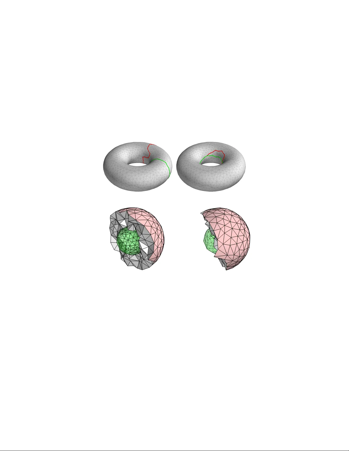
Optimal Homologous Cycles, Total Unimodularity, and Linear Programming

Optimal Homologous Cycles, T otal Unimodularity , and Linear Programming ∗ T amal K. Dey † Anil N. Hirani ‡ Bala Krishnamoorthy § Abstract Giv en a simplicial complex with weights on its simplices, and a nontrivial cycle on it, we are inter- ested in finding the cycle with minimal weight which is homologous to the giv en one. Assuming that the homology is defined with integer ( Z ) coef ficients, we sho w the following (Theorem 5.2): F or a finite simplicial comple x K of dimension gr eater than p , the boundary matrix [ ∂ p +1 ] is totally unimodular if and only if H p ( L, L 0 ) is torsion-fr ee, for all pure subcomplexes L 0 , L in K of dimensions p and p + 1 r espectively , wher e L 0 ⊂ L . Because of the total unimodularity of the boundary matrix, we can solve the optimization problem, which is inherently an integer programming problem, as a linear program and obtain an integer solution. Thus the problem of finding optimal c ycles in a giv en homology class can be solved in polynomial time. This result is surprising in the backdrop of a recent result which says that the problem is NP-hard under Z 2 coefficients which, being a field , is in general easier to deal with. Our result implies, among other things, that one can compute in polynomial time an optimal ( d − 1) -cycle in a giv en homology class for any triangulation of an orientable compact d -manifold or for any finite simplicial complex embedded in R d . Our optimization approach can also be used for various related problems, such as finding an optimal chain homologous to a given one when these are not cycles. Our result can also be viewed as providing a topological characterization of total unimodularity . 1 Intr oduction T opological cycles in shapes embody their important features. As a result they find applications in scientific studies and engineering dev elopments. A version of the problem that often appears in practice is that gi ven a cycle in the shape, compute the shortest cycle in the same topological class (homologous). For example, one may generate a set of cycles from a simplicial complex using the persistence algorithm [10] and then ask to tighten them while maintaining their homology classes. For two dimensional surfaces, this problem and its relati v es ha ve been widely studied in recent years; see, for example, [2, 3, 5, 6, 8]. A natural question is to consider higher dimensional spaces which allow higher dimensional cycles such as closed surfaces within a three dimensional topological space. High dimensional applications arise, for example, in the modeling of sensor networks by V ietoris-Rips complexes of arbitrary dimension [7, 20]. Not surprisingly , these generalizations are hard to compute which is confirmed by a recent result of Chen and Freedman [4]. Notwithstanding this neg ativ e development, our result shows that optimal homologous cycles in any finite ∗ A preliminary version of this paper appeared in the Proceedings of 42nd A CM Symposium on Theory of Computing, 2010. † Department of Computer Science and Engineering, The Ohio State Univ ersity , Columbus, OH 43210, USA. tamaldey@cse.ohio-state.edu , http://www.cse.ohio- state.edu/ ˜ tamaldey ‡ Department of Computer Science, Univ ersity of Illinois at Urbana-Champaign, IL 61801, USA. hirani@cs.illinois.edu , http://www.cs.illinois.edu/hirani § Department of Mathematics, W ashington State Univ ersity , Pullman, W A 99164, USA. bkrishna@math.wsu.edu , http://www.math.wsu.edu/math/faculty/bkrishna 1 dimension are polynomial time computable for a lar ge class of shapes if homology is defined with integer coef ficients. Let K be a simplicial complex. Informally , a p -cycle in K is a collection of p -simplices whose bound- aries cancel mutually . One may assign a non-zero weight to each p -simplex in K which induces a weighted 1-norm for each p -cycle in K . F or example, the weight of a p -simplex could be its volume. Gi ven an y p -cycle c in K , our problem is to compute a p -cycle c ∗ which has the minimal weighted 1-norm in the homology class of c . If some of the weights are zero the problem can still be posed and solved, except that one may not call it weighted 1-norm minimization. The homology classes are defined with respect to coef ficients in an abelian group such as Q , R , Z , Z n etc. Often, the group Z 2 is used mainly because of simplicity and intuiti ve geometric interpretations. Chen and Freedman [4] show that under Z 2 coef ficients, computing an optimal p -cycle c ∗ is NP-hard for p ≥ 1 . Moreo ver , their result implies that various relaxations may still be NP-hard. For example, computing a constant factor approximation of c ∗ is NP-hard. Even if the rank of the p -dimensional homology group is constant, computing c ∗ remains NP-hard for p ≥ 2 . The only settled positiv e case is a result of Chambers, Erickson, and Nayyeri [3] who sho w that computing optimal homologous loops for surfaces with constant genus is polynomial time solv able though they prov e the problem is NP-hard if the genus is not a constant. The above negati ve results put a roadblock in computing optimal homologous cycles in high dimensions. Fortunately , our result shows that it is not so hopeless – if we switch to the coefficient group Z instead of Z 2 , the problem becomes polynomial time solv able for a fairly lar ge class of spaces. This is a little surprising gi ven that Z is not a field and so seems harder to deal with than Z 2 in general. F or example, Z 2 -v alued chains form a vector space, b ut Z -v alued chains do not. The problem of computing an optimal homologous c ycle (or more generally , chain) can be cast as a lin- ear optimization problem. Consequently , the problem becomes polynomial time solvable if the homology group is defined ov er the reals, since it can be solved by linear programming. Indeed this is the approach taken by T ahbaz-Salehi and Jadbabaie [20]. Howe ver , in general the optimal cycle in that case may hav e fractional coef ficients for its simplices, which may be awkward in certain applications. One advantage of using Z is that simplices appear with integral coef ficients in the solution. On the other hand, the linear programming has to be replaced by integer programming in the case of Z . Thus, it is not immediately clear if the optimization problem is polynomial time solvable. One issue in accommodating Z as the coefficient ring is that integral coefficients other than 0 , 1 , or − 1 do not ha ve natural geometric meaning. Nev erthe- less, our experiments suggest that optimal solutions in practice may contain coefficients only in {− 1 , 0 , 1 } . Furthermore, as we sho w later , we can put a constraint in our optimization to enforce the solution to hav e coef ficients in {− 1 , 0 , 1 } . Our main observ ation is that the optimization problem that we formulate can be solved by linear pro- gramming under certain conditions, although it is inherently an integer programming problem. It is known that a linear program provides an integer solution if and only if the constraint matrix has a property called total unimodularity . A matrix is totally unimodular if and only if each of its square submatrices has a de- terminant of 0 , 1 , or − 1 . W e give a precise topological characterization of the complex es for which the constraint matrix is totally unimodular . For this class of complexes the optimal c ycle can be computed in time polynomial in the number of simplices. T otally unimodular matrices ha ve a well-kno wn geometric characterization – that the corresponding constraint polyhedron is integral [15, Theorem 19.1]. Our result provides a topological characterization as well. W e can allow se veral variations to our problem because of our optimization based approach. For ex- ample, we can probe into intermediate solutions; we can produce the chain that bounds the difference of the input and optimal cycles, and so forth. In fact, we can also find an optimal chain homologous to a gi ven one when the chains are not cycles. In other words, we can lev erage the flexibility of the optimiza- tion formulation by linking results from two apparently dif ferent fields, optimization theory and algebraic topology . 2 2 Backgr ound Since our result bridges the two v ery dif ferent fields of algebraic topology and optimization, we recall some rele vant basic concepts and definitions from these tw o fields. 2.1 Basic definitions from algebraic topology Let K be a finite simplicial complex of dimension greater than p . A p -chain with Z coefficients in K is a formal sum of a set of oriented p -simplices in K where the sum is defined by addition in Z . Equiv alently , it is an integer v alued function on the oriented p -simplices, which changes sign when the orientation is rev ersed [14, page 37]. T wo p -chains can be added by adding their values on corresponding p -simplices, resulting in a group C p ( K ) called the p -chain group of K . The elementary chain basis for C p ( K ) is the one consisting of integer v alued functions that take the value 1 on a single oriented p -simplex, − 1 on the oppositely oriented simplex, and 0 ev erywhere else. For an oriented p -simplex σ , we use σ to denote both the simplex and the corresponding elementary chain basis element. The group C p ( K ) is free and abelian. The boundary of an oriented p -simplex σ = [ v 0 , . . . , v p ] is gi ven by ∂ p σ = p X i =0 ( − 1) i [ v 0 , .., b v i , .., v p ] , where b v i denotes that the verte x v i is to be deleted. This function on p -simplices extends uniquely [14, page 28] to the boundary operator which is a homomorphism: ∂ p : C p ( K ) → C p − 1 ( K ) . Like a linear operator between vector spaces, a homomorphism between free abelian groups has a unique matrix representation with respect to a choice of bases [14, page 55]. The matrix form of ∂ p will be denoted [ ∂ p ] . Let { σ i } m − 1 i =0 and { τ j } n − 1 j =0 be the sets of oriented ( p − 1) - and p -simplices respectively in K , ordered arbitrarily . Thus { σ i } and { τ j } also represent the elementary chain bases for C p − 1 ( K ) and C p ( K ) respec- ti vely . W ith respect to such bases [ ∂ p ] is an m × n matrix with entries 0, 1 or − 1 . The coefficients of ∂ p τ j in the C p − 1 ( K ) basis become the column j (counting from 0) of [ ∂ p ] . The kernel k er ∂ p is called the group of p - cycles and denoted Z p ( K ) . The image im ∂ p +1 forms the group of p - boundaries and denoted B p ( K ) . Both Z p ( K ) and B p ( K ) are subgroups of C p ( K ) . Since ∂ p ◦ ∂ p +1 = 0 , we have that B p ( K ) ⊆ Z p ( K ) , that is, all p -boundaries are p -cycles though the con verse is not necessarily true. The p dimensional homology group is the quotient group H p ( K ) = Z p ( K ) /B p ( K ) . T wo p -chains c and c 0 in K are homolo gous if c = c 0 + ∂ p +1 d for some ( p + 1) -chain d in K . In particular , if c = ∂ p +1 d , we say c is homologous to zero. If a c ycle c is not homologous to zero, we call it a non-trivial cycle . For a finite simplicial complex K , the groups of chains C p ( K ) , cycles Z p ( K ) , and H p ( K ) are all finitely generated abelian groups. By the fundamental theorem of finitely generated abelian groups [14, page 24] any such group G can be written as a direct sum of two groups G = F ⊕ T where F ∼ = ( Z ⊕ · · · ⊕ Z ) and T ∼ = ( Z /t 1 ⊕ · · · ⊕ Z /t k ) with t i > 1 and t i di viding t i +1 . The subgroup T is called the torsion of G . If T = 0 , we say G is torsion-fr ee . Let L 0 be a subcomplex of a simplicial complex L . The quotient group C p ( L ) /C p ( L 0 ) is called the group of r elative chains of L modulo L 0 and is denoted C p ( L, L 0 ) . The boundary operator ∂ p : C p ( L ) → C p − 1 ( L ) and its restriction to L 0 induce a homomorphism ∂ ( L,L 0 ) p : C p ( L, L 0 ) → C p − 1 ( L, L 0 ) . 3 As before, we have ∂ ( L,L 0 ) p ◦ ∂ ( L,L 0 ) p +1 = 0 . Writing Z p ( L, L 0 ) = ker ∂ ( L,L 0 ) p for r elative cycles and B p ( L, L 0 ) = im ∂ ( L,L 0 ) p +1 for r elative boundaries , we obtain the r elative homology gr oup H p ( L, L 0 ) = Z p ( L, L 0 ) /B p ( L, L 0 ) . Sometimes, to distinguish it from relative homology , the usual homology H p ( L ) is called the absolute homology gr oup of L . 2.2 T otal unimodularity and optimization Recall that a matrix is totally unimodular if the determinant of each square submatrix is 0 , 1 , or − 1 . The significance of total unimodularity in our setting is due to the follo wing result: Theorem 2.1. [24] Let A be an m × n totally unimodular matrix and b an inte gral vector , i.e., b ∈ Z m . Then the polyhedr on P := { x ∈ R n | A x = b , x ≥ 0 } is integr al, meaning that P is the con vex hull of the integr al vectors contained in P . In particular , the extr eme points (vertices) of P ar e inte gral. Similarly the polyhedr on Q := { x ∈ R n | A x ≥ b } is inte gral. The following corollary shows why the above result is significant for optimization problems. Consider an inte gral v ector b ∈ Z m and a real v ector of cost coef ficients f ∈ R n . Consider the inte ger linear program min f T x subject to A x = b , x ≥ 0 and x ∈ Z n . (1) Corollary 2.2. Let A be a totally unimodular matrix. Then the inte ger linear pr ogram (1) can be solved in time polynomial in the dimensions of A . Pr oof. Relax the integer linear program (1) to a linear program by removing the integrality constraint x ∈ Z n . Then an interior point method for solving linear programs will find a real solution x ∗ in polynomial time [15] if it exists, and indicates the unboundedness or infeasibility of the linear program otherwise. In fact, since the matrix A has entries 0, 1 or − 1 , one can solv e the linear program in strongly polynomial time [21, 22]. That is, the number of arithmetic operations do not depend on b and f and solely depends on the dimension of A . One still needs to sho w that the solution x ∗ is integral. If the solution is unique then it lies at a vertex of the polyhedron P and thus it will be integral because of Theorem 2.1. If the optimal solution set is a face of P which is not a v ertex then an interior point method may at first find a non-integral solution. Ho we ver , by [1, Corollary 2.2] the polyhedron P must ha ve at least one vertex. Then, by [1, Theorem 2.8] if the optimal cost is finite, there exists a vertex of P where that optimal cost is achiev ed. Follo wing the procedure described in [12], starting from the possibly non-integral solution obtained by an interior point method one can find such an integral optimal solution at a vertex in polynomial time. 3 Pr oblem formulation Let K be a finite simplicial complex of dimension p or more. Gi ven an integer v alued p -chain x = P m − 1 i =0 x ( σ i ) σ i we use x ∈ Z m to denote the vector formed by the coefficients x ( σ i ) . Thus, x is the representation of the chain x in the elementary p -chain basis, and we will use x and x interchangeably . For a vector v ∈ R m , the 1-norm (or ` 1 -norm) k v k 1 is defined to be P i | v i | . Let W be an y real m × m diagonal matrix with diagonal entries w i . Then, the 1-norm of W v , that is, k W v k 1 is P i | w i || v i | . (If W is a general m × m nonsingular matrix then k W v k 1 is called the weighted 1-norm of v .) The norm or weighted norm of an integral vector v ∈ Z m is defined by considering v to be in R m . W e now state in words the problem of optimal homologous chains and later formalize it in (2): Gi ven a p -chain c in K and a diagonal matrix W of appropriate dimension, the optimal ho- mologous chain problem (OHCP) is to find a chain c ∗ which has the minimal 1-norm k W c ∗ k 1 among all chains homologous to c . 4 Remark 3.1 . In the natural case where simplices are weighted and the optimality of the chains is to be determined with respect to these weights, we may take W to be diagonal with w i being the weight of simplex σ i . In our formulation some of the weights can be 0. Notice that the signs of the simplex weights are ignored in our formulation since we only work with norms. Remark 3.2 . In Section 1 we surveyed the computational topology literature on the problem of finding optimal homologous cycles . The flexibility of our formulation allows us to solve the more general, opti- mal homologous c hain problem, with the cycle case being a special case requiring no modification in the equations, algorithm, or theorems. Remark 3.3 . The choice of 1-norm is important. At first, it might seem easier to pose OHCP using 2- norm. Then, calculus can be used to pose the minimization as a stationary point problem when OHCP is formulated with only equality constraints which appear in (2) below . This case can be solved as a linear system of equations. By using 1-norm instead of 2-norm, we hav e to solve a linear program (as we will sho w below) instead of a linear system. But in return, we are able to get integer valued solutions when the appropriate conditions are satisfied. The formulation of OHCP is the weighted ` 1 -optimization of homologous chains. This is very general and allows for dif ferent types of optimality to be achie ved by choosing different weight matrices. For example, assume that the simplicial complex K of dimension greater than p is embedded in R d , where d ≥ p + 1 . Let W be a diagonal matrix with the i -th diagonal entry being the Euclidean p -dimensional volume of a p -simplex. This specializes the problem to the Euclidean ` 1 -optimization problem. The resulting optimal chain has the smallest p -dimensional v olume amongst all chains homologous to the giv en one. If W is taken to be the identity matrix, with appropriate additional conditions to the above formulation, one can solve the ` 0 -optimization problem. The resulting optimal solution has the smallest number of p -simplices amongst all chains homologous to c , as we sho w in Section 3.2. The centr al idea of this paper consists of the following steps : (i) write OHCP as an integer program in v olving 1-norm minimization, subject to linear constraints; (ii) con vert the inte ger program into an integer linear program by con verting the 1-norm cost function to a linear one using the standard technique of introducing some extra variables and constraints; (iii) find the conditions under which the constraint matrix of the inte ger linear program is totally unimodular; and (iv) for this class of problems, relax the inte ger linear program to a linear program by dropping the constraint that the variables be integral. The resulting optimal chain obtained by solving the linear program will be an integer v alued chain homologous to the gi ven chain. 3.1 Optimal homologous chains and linear programming No w we formally pose OHCP as an optimization problem. After sho wing existence of solutions we refor - mulate the optimization problem as an integer linear program and e ventually as a linear program. Assume that the number of p - and ( p + 1) -simplices in K is m and n respectiv ely , and let W be a diagonal m × m matrix. Gi ven an integer valued p -chain c the optimal homologous chain problem is to solve: min x , y k W x k 1 such that x = c + [ ∂ p +1 ] y , and x ∈ Z m , y ∈ Z n . (2) In the problem formulation (2) we hav e given no indication of the algorithm that will be used to solve the problem. Before we dev elop the computational side, it is important to show that a solution to this problem always e xists. Claim 3.4. F or any given p -chain c and any matrix W , the solution to pr oblem (2) exists. Pr oof. Define the set U c := {k W x k 1 | x = c + [ ∂ p +1 ] y , x ∈ Z m and y ∈ Z n } . 5 W e show that this set has a minimum which is contained in the set. Consider the subset U 0 c ⊆ U c defined by U 0 c = {k W x k 1 | k W x k 1 ≤ k W c k 1 , x = c + [ ∂ p +1 ] y , x ∈ Z m and y ∈ Z n } . This set U 0 c is finite since x is integral. Therefore, inf U c = inf U 0 c = min U 0 c . In the rest of this paper we assume that W is a diagonal matrix obtained from weights on simplices as follows. Let w be a real-valued weight function on the oriented p -simplices of K and let W be the corresponding diagonal matrix (the i -th diagonal entry of W is w ( σ i ) = w i ). The resulting objecti ve function k W x k 1 = P i | w i | | x i | in (2) is not linear in x i because it uses the absolute value of x i . It is howe ver , piecewise-linear in these v ariables. As a result, (2) can be reformulated as an integer linear program in the following standard w ay [1, page 18]: min X i | w i | ( x + i + x − i ) subject to x + − x − = c + [ ∂ p +1 ] y (3) x + , x − ≥ 0 x + , x − ∈ Z m , y ∈ Z n . Comparing the abo ve formulation to the standard form inte ger linear program in (1), note that the vector x in (1) corresponds to [ x + , x − , y ] T in (3) above. Thus the minimization is over x + , x − and y , and the coef ficients of x + i and x − i in the objecti ve function are | w i | , but the coef ficients corresponding to y j are zero. The linear programming relaxation of this formulation just removes the constraints about the v ariables being integral. The resulting linear program is: min X i | w i | ( x + i + x − i ) subject to x + − x − = c + [ ∂ p +1 ] y (4) x + , x − ≥ 0 . T o use the result about standard form polyhedron in Theorem 2.1 we can eliminate the free (unrestricted in sign) variables y by replacing these by y + − y − and imposing the non-negati vity constraints on the ne w variables [1, page 5]. The resulting linear program has the same objectiv e function, and the equality constraints: x + − x − = c + [ ∂ p +1 ] ( y + − y − ) , (5) and thus the equality constraint matrix is  I − I − B B  , where B = [ ∂ p +1 ] . W e now pro ve a result about the total unimodularity of this matrix. Lemma 3.5. If B = [ ∂ p +1 ] is totally unimodular then so is the matrix  I − I − B B  . Pr oof. The proof uses operations that preserve the total unimodularity of a matrix. These are listed in [15, page 280]. If B is totally unimodular then so is the matrix  − B B  since scalar multiples of columns of B are being appended on the left to get this matrix. The full matrix in question can be obtained from this one by appending columns with a single ± 1 on the left, which prov es the result. As a result of Corollary 2.2 and Lemma 3.5, we hav e the follo wing algorithmic result. Theorem 3.6. If the boundary matrix [ ∂ p +1 ] of a finite simplicial complex of dimension gr eater than p is totally unimodular , the optimal homologous chain pr oblem (2) for p -chains can be solved in polynomial time. 6 Pr oof. W e hav e seen abov e that a reformulation of OHCP (2), without the integrality constraints, leads to the linear program (4). By Lemma 3.5, the equality constraint matrix of this linear program is totally unimodular . Then by Corollary 2.2 the linear program (4) can be solved in polynomial time, while achie ving an integral solution. Remark 3.7 . One may wonder why Theorem 3.6 does not work when Z 2 -v alued chains are considered instead of integer-v alued chains. W e could simulate Z 2 arithmetic while using integers or reals by modify- ing (2) as follo ws: min x , y k W x k 1 such that x + 2 u = c + [ ∂ p +1 ] y , and x ∈ { 0 , 1 } m , u ∈ Z m , y ∈ Z n . (6) The trouble is that the coef ficient 2 of u destroys the total unimodularity of the constraint matrix in the linear programming relaxation of the above formulation, e ven when [ ∂ p +1 ] is totally unimodular . Thus we cannot solve the abo ve inte ger program as a linear program and still get integer solutions. Remark 3.8 . W e can associate weights with ( p + 1) -simplices while formulating the optimization prob- lem (2). Then, we could minimize k W z k 1 where z = [ x , y ] T . In that case, we obtain a p -chain c ∗ ho- mologous to the giv en chain c and also a ( p + 1) -chain d whose boundary is c ∗ − c and the weights of c ∗ and d together are the smallest. If the given cycle c is null homologous, the optimal y would be an optimal ( p + 1) -chain bounded by c . Remark 3.9 . The simple x method and its variants search only the basic feasible solutions (vertices of the constraint polyhedron), while choosing ones that ne ver make the objectiv e function worse. Thus if the polyhedron is integral, one could stop the simplex method at any step before reaching optimality and still obtain an integer v alued homologous chain whose norm is no worse than that of the gi ven chain. 3.2 Minimizing the number of simplices The general weighted ` 1 -optimization problem (2) can be specialized by choosing different weight matrices. One can also solve v ariations of the OHCP problem by adding other constraints which do not destroy the total unimodularity of the constraint matrix. W e consider one such specialization here – that of finding a homologous chain with the smallest number of simplices. If the matrix W is chosen to be the identity matrix, then one can solve the ` 0 -optimization problem by solving a modified version of the ` 1 -optimization problem (2). One just imposes the extra condition that ev ery entry of c and x be in {− 1 , 0 , 1 } . W ith this choice of W = I and with c ∈ {− 1 , 0 , 1 } m , the problem (2) becomes: min x , y k x k 1 such that x = c + [ ∂ p +1 ] y , and x ∈ {− 1 , 0 , 1 } m , y ∈ Z n . (7) Theorem 3.10. F or any given p -chain c ∈ {− 1 , 0 , 1 } m , a solution to pr oblem (7) exists. Furthermor e, amongst all x homologous to c , the optimal homologous chain x ∗ has the smallest number of nonzer o entries, that is, it is the ` 0 -optimal homologous c hain. Pr oof. The proof of e xistence is identical to the proof of Claim 3.4. The condition that c takes v alues in − 1 , 0, 1 ensures that at least x = c can be taken as the solution if no other homologous chain exists. For the ` 0 -optimality , note that since the entries of the optimal solution x ∗ are constrained to be in {− 1 , 0 , 1 } , the 1-norm measures the number of nonzero entries. Thus the 1-norm optimal solution is also the one with the smallest number of non-zero entries. Remark 3.11 . Note that e ven with the gi ven chain c taking v alues in {− 1 , 0 , 1 } , without the e xtra constraint that x ∈ {− 1 , 0 , 1 } m (rather than just x ∈ Z m ), the optimal 1-norm solution components may take values 7 outside {− 1 , 0 , 1 } . F or example, consider the simplicial complex K triangulating a cylinder which is shaped like an hour glass. Let c 1 and c 2 be the two boundary cycles of the hour glass so that c 1 + c 2 is not trivial. Let z be the smallest cycle around the middle of the hour glass which is homologous to each of c 1 and c 2 . Since c 1 + c 2 = 2 z , the optimal c ycle homologous to c 1 + c 2 has v alues 2 or − 2 for some edges ev en if c 1 and c 2 hav e values only in {− 1 , 0 , 1 } for all edges. It may or may not be true that the number of nonzero entries is minimal in such an optimal solution. W e hav e not prov ed it either way . But Theorem 3.10 provides a guarantee for computing ` 0 -optimal solution when the additional constraints are placed on x . The linear programming relaxation of problem (7) is min X i ( x + i + x − i ) subject to x + − x − = c + [ ∂ p +1 ] y (8) x + , x − ≤ 1 x + , x − ≥ 0 . One can show the integrality of the feasible set polyhedron by using slack v ariables to conv ert the inequal- ities x + ≤ 1 and x − ≤ 1 to equalities and then using the P form of the polyhedron from Theorem 2.1. Equi valently , all the constraints can be written as inequalities and the Q polyhedron can be used. For a change we choose the latter method here. Writing the constraints as inequalities, in matrix form the con- straints are             − I I B − B I − I − B B − I 0 0 0 0 − I 0 0 I 0 0 0 0 I 0 0 0 0 I 0 0 0 0 I                 x + x − y + y −     ≥             − c c − 1 − 1 0 0 0 0             , (9) where B = [ ∂ p +1 ] . Then analogously to Lemma 3.5 and Theorem 3.6 the follo wing are true. Lemma 3.12. If B = [ ∂ p +1 ] is totally unimodular then so is the constraint matrix in (9) . Theorem 3.13. If the boundary matrix [ ∂ p +1 ] of a finite simplicial complex of dimension gr eater than p is totally unimodular , then given a p -chain that takes values in {− 1 , 0 , 1 } , a homologous p -chain with the smallest number of non-zer os taking values in {− 1 , 0 , 1 } can be found in polynomial time. In subsequent sections, we characterize the simplicial complex es for which the boundary matrix [ ∂ p +1 ] is totally unimodular . These are the main theoretical results of this paper , formalized as Theorems 4.1, 5.2, and 5.7. 4 Manif olds Our results in Section 5.1 are v alid for any finite simplicial complex. But first we consider a simpler case – simplicial complex es that are triangulations of manifolds. W e sho w that for finite triangulations of compact p -dimensional orientable manifolds, the top non-tri vial boundary matrix [ ∂ p ] is totally unimodular irrespec- ti ve of the orientations of its simplices. W e also giv e examples of non-orientable manifolds where total unimodularity does not hold. Further examination of why total unimodularity does not hold in these cases leads to our main results in Theorems 5.2. 8 4.1 Orientable manif olds Let K be a finite simplicial complex that triangulates a ( p + 1) -dimensional compact orientable manifold M . As before, let [ ∂ p +1 ] be the matrix corresponding to ∂ p +1 : C p +1 ( K ) → C p ( K ) in the elementary chain bases. Theorem 4.1. F or a finite simplicial comple x triangulating a ( p + 1) -dimensional compact orientable man- ifold, [ ∂ p +1 ] is totally unimodular irr espective of the orientations of the simplices. Pr oof. First, we pro ve the theorem assuming that the ( p + 1) -dimensional simplices of K are oriented consistently . Then, we argue that the result still holds when orientations are arbitrary . Consistent orientation of ( p + 1) -simplices means that they are oriented in such a way that for the ( p + 1) - chain c , which tak es the value 1 on each oriented ( p + 1) -simplex in K , ∂ p +1 c is carried by the topological boundary ∂ M of M . If M has no boundary then ∂ p +1 c is 0. It is known that consistent orientation of ( p + 1) -simplices alw ays exists for a finite triangulation of a compact orientable manifold. Therefore, assume that the giv en triangulation has consistent orientation for the ( p + 1) -simplices. The orientation of the p - and lo wer dimensional simplices can be chosen arbitrarily . Each p -face τ is the face of either one or two ( p + 1) -simplices (depending on whether τ is a boundary face or not). Thus the ro w of [ ∂ p +1 ] corresponding to τ contains one or two nonzeros. Such a nonzero entry is 1 if the orientation of τ agrees with that of the corresponding ( p + 1) -simplex and − 1 if it does not. Heller and T ompkins [13] ga ve a sufficient condition for the unimodularity of {− 1 , 0 , 1 } -matrices whose columns hav e no more than two nonzero entries. Such a matrix is totally unimodular if its ro ws can be di- vided into two partitions (one possibly empty) with the following condition. If two nonzeros in a column belong to the same partition, they must be of opposite signs, otherwise they must be in different row par - titions. Consider [ ∂ p +1 ] T , the transpose of [ ∂ p +1 ] . Each column of [ ∂ p +1 ] T contains at most two nonzero entries, and if there are two then they are of opposite signs because of the consistent orientations of the ( p + 1) -dimensional simplices. In this case, the simple di vision of rows into two partitions with one con- taining all ro ws and the other empty works. Thus [ ∂ p +1 ] T and hence [ ∂ p +1 ] is totally unimodular . No w , re versing the orientation of a ( p + 1) -simplex means that the corresponding column of [ ∂ p +1 ] be multiplied by − 1 . This column operation preserves the total unimodularity of [ ∂ p +1 ] . Since any arbi- trary orientation of the ( p + 1) -simplices can be obtained by preserving or rev ersing their orientations in a consistent orientation, we hav e the result as claimed. As a result of the abov e theorem and Theorem 3.6 we hav e the following result. Corollary 4.2. F or a finite simplicial complex triangulating a ( p + 1) -dimensional compact orientable manifold, the optimal homologous chain pr oblem can be solved for p -dimensional chains in polynomial time. The result in Corollary 4.2 when specialized to R p +1 also appears in [19] though the reasoning is differ - ent. 4.2 Non-orientable manif olds For non-orientable manifolds we give two e xamples which sho w that total unimodularity may not hold in this case. W e also discuss the role of torsion in these examples in preparation for Theorem 5.2. Our first example is the M ¨ obius strip and the second one is the projective plane. Simplicial complex es for these tw o non-orientable surfaces are shown in Figure 1. The boundary matrices [ ∂ 2 ] for these simplicial complex es are giv en in the Appendix in (11) and (12). Let M be the M ¨ obius strip. W e consider its absolute homology H 1 ( M ) and its relati ve homology H 1 ( M , ∂ M ) relative to its boundary . Consult [14, page 135] to see how the various homology groups are 9 10 6 11 1 5 7 2 4 9 2 3 0 4 1 0 0 3 5 8 5 5 0 4 3 1 10 11 12 7 8 6 13 9 3 8 4 1 0 0 1 2 7 5 2 14 9 6 Figure 1: Triangulations of two non-orientable manifolds, shown as abstract simplicial complex es. The left figure shows a triangulation of the M ¨ obius strip and the right one shows the projectiv e plane. The numbers are the edge and triangles numbers. These correspond to the row and column numbers of the matrices (11) and (12). calculated using an e xact sequence. W e note that H 1 ( M ) ∼ = Z , that is, its H 1 group has no torsion. This can be seen by reducing the matrix (11) in the Appendix to Smith normal form (SNF). The SNF for the matrix consists of a 6 × 6 identity matrix on the top and a zero block below , which implies the absence of torsion. Let K be the simplicial complex triangulating M . Consider a submatrix S of the matrix [ ∂ 2 ] shown in Appendix as (11). This submatrix is formed by selecting the columns in the order 5, 4, 3, 2, 1, 0. From the matrix thus formed, select the rows 0, 3, 8, 9, 10, 2 in that order . This selection of rows and columns corresponds to all the triangles and the edges encountered as one goes from left to right in the M ¨ obius triangulation sho wn in Figure 1. The resulting submatrix is S =         1 0 0 0 0 1 − 1 1 0 0 0 0 0 − 1 1 0 0 0 0 0 − 1 1 0 0 0 0 0 − 1 1 0 0 0 0 0 1 − 1         The determinant of this matrix is − 2 and this shows that the boundary matrix is not totally unimodular . The SNF for this matrix, it turns out, does reveal the torsion. This matrix S is the relativ e boundary matrix ∂ ( L,L 0 ) 2 where L = K and L 0 are the edges in ∂ M . The SNF has 1’ s along the diagonal and finally a 2. This is an example where there is no torsion in the absolute homology but some torsion in the relativ e homology and the boundary matrix is not totally unimodular . W e formulate this condition precisely in Theorem 5.2. The matrix [ ∂ 2 ] gi ven in Appendix as (12) for the projectiv e plane triangulation is much lar ger . But it is easy to find a submatrix with determinant greater than 1. This can be done by finding the M ¨ obius strip in the triangulation of the projecti ve plane. For example if one trav erses from top to bottom in the triangulation of the projecti ve plane in Figure 1 the triangles encountered correspond to columns 6, 9, 3, 8, 4 of (12) and the 10 edges correspond to ro ws 5, 11, 13, 12, 7. The corresponding submatrix is S =       − 1 0 0 0 − 1 − 1 1 0 0 0 0 − 1 1 0 0 0 0 − 1 1 0 0 0 0 − 1 1       and its determinant is − 2 . Thus the boundary matrix (12) is not totally unimodular . Again, we observe that there is relati ve torsion in H 1 ( L, L 0 ) for the subcomplex es corresponding to the selection of S from [ ∂ 2 ] . Here L consists of the triangles specified abov e, which form a M ¨ obius strip in the projectiv e plane. The subcomplex L 0 consists of the edges forming the boundary of this strip. This connection between submatrices and relati ve homology is examined in the ne xt section. 5 Simplicial complexes No w we consider the more general case of simplicial complex es. Our result in Theorem 5.2 characterizes the total unimodularity of boundary matrices for arbitrary simplicial complex es. Since we do not use any conditions about the geometric realization or embedding in R n for the complex, the result is also v alid for abstract simplicial complexes. As a corollary of the characterization we show that the OHCP can be solved in polynomial time as long as the input complex satisfies a torsion-related condition. 5.1 T otal unimodularity and relati ve torsion Let K be a finite simplicial complex of dimension greater than p . W e will need to refer to its subcomplex es formed by the union of some of its simplices of a specific dimension. This is formalized in the definition belo w . Definition 5.1. A pur e simplicial comple x of dimension p is a simplicial comple x formed by a collection of p -simplices and their proper faces. Similarly , a pur e subcomplex is a subcomplex that is a pure simplicial complex. An example of a pure simplicial complex of dimension p is one that triangulates a p -dimensional man- ifold. Another example, relev ant to our discussion, is a subcomplex formed by a collection of some p - simplices of a simplicial complex and their lo wer dimensional faces. Let L ⊆ K be a pure subcomplex of dimension p + 1 and L 0 ⊂ L be a pure subcomplex of dimension p . If [ ∂ p +1 ] is the matrix representing ∂ p +1 : C p +1 ( K ) → C p ( K ) , then the matrix representing the relative boundary operator ∂ ( L,L 0 ) p +1 : C p +1 ( L, L 0 ) → C p ( L, L 0 ) , is obtained by first including the columns of [ ∂ p +1 ] corresponding to ( p + 1) -simplices in L and then, from the submatrix so obtained, e xcluding the rows corresponding to the p -simplices in L 0 and any zero ro ws. The zero ro ws correspond to p -simplices that are not faces of any of the ( p + 1) -simplices of L . As before, let [ ∂ p +1 ] be the matrix of ∂ p +1 in the elementary chain bases for K . Then the follo wing holds. Theorem 5.2. [ ∂ p +1 ] is totally unimodular if and only if H p ( L, L 0 ) is torsion-fr ee, for all pur e subcomplexes L 0 , L of K of dimensions p and p + 1 respectively , wher e L 0 ⊂ L . 11 Pr oof. ( ⇒ ) W e show that if H p ( L, L 0 ) has torsion for some L, L 0 then [ ∂ p +1 ] is not totally unimodular . Let h ∂ ( L,L 0 ) p +1 i be the corresponding relativ e boundary matrix. Bring h ∂ ( L,L 0 ) p +1 i to Smith normal form using the reduction algorithm [14][pages 55–57]. This is a block matrix  D 0 0 0  where D = diag ( d 1 , . . . , d l ) is a diagonal matrix and the block row or column of zero matrices shown abov e may be empty , depending on the dimension of the matrix. Recall that d i are integers and d i ≥ 1 . Moreov er , since H p ( L, L 0 ) has torsion, d k > 1 for some 1 ≤ k ≤ l . Thus the product d 1 . . . d k is greater than 1. By a result of Smith [17] quoted in [15, page 50], this product is the greatest common di visor of the determinants of all k × k square submatrices of h ∂ ( L,L 0 ) p +1 i . But this implies that some square submatrix of h ∂ ( L,L 0 ) p +1 i , and hence of [ ∂ p +1 ] , has determinant magnitude greater than 1. Thus [ ∂ p +1 ] is not totally unimodular . ( ⇐ ) Assume that [ ∂ p +1 ] is not totally unimodular . W e will show that then there exist subcomplexes L 0 and L of dimensions p and ( p + 1) respectiv ely , with L 0 ⊂ L , such that H p ( L, L 0 ) has torsion. Let S be a square submatrix of [ ∂ p +1 ] such that | det( S ) | > 1 . Let L correspond to the columns of [ ∂ p +1 ] that are included in S and let B L be the submatrix of [ ∂ p +1 ] formed by these columns. This submatrix B L may contain zero rows. Those zero rows (if any) correspond to p -simplices that do not occur as a face of any of the ( p + 1) -simplices in L . In order to form S from B L , these zero ro ws can first be safely discarded to form a submatrix B 0 L . This is because det( S ) 6 = 0 and so these zero rows cannot occur in S . The ro ws in B 0 L correspond to p -simplices that occur as a face of some ( p + 1) -simplex in L . Let L 0 correspond to rows of B 0 L which are excluded to form S . Now S is the matrix representation of the relativ e boundary matrix ∂ ( L,L 0 ) p . Reduce S to Smith normal form. The normal form is a square diagonal matrix. Since the elementary ro w and column operations preserve determinant magnitude, the determinant of the resulting diagonal matrix has magnitude greater than 1. Thus at least one of the diagonal entries in the normal form is greater than 1. But then by [14, page 61] H p ( L, L 0 ) has torsion. Remark 5.3 . The characterization appears to be no easier to check than the definition of total unimodularity since it in volv es checking every L, L 0 pair . Ho we ver , it is also no harder to check than total unimodularity . This leads to the follo wing result of possible interest in computational topology and matroid theory . Corollary 5.4. F or a simplicial complex K of dimension gr eater than p , ther e is a polynomial time algo- rithm for answering the following question: Is H p ( L, L 0 ) tor sion-fr ee for all subcomple xes L 0 and L of dimensions p and ( p + 1) such that L 0 ⊂ L ? Pr oof. Seymour’ s decomposition theorem for totally unimodular matrices [16],[15, Theorem 19.6] yields a polynomial time algorithm for deciding if a matrix is totally unimodular or not [15, Theorem 20.3]. That algorithm applied on the boundary matrix [ ∂ p +1 ] prov es the abov e assertion. Remark 5.5 . Note that the nai v e algorithm for the abo ve problem is clearly e xponential. F or e very pair L, L 0 one can use a polynomial time algorithm to find the Smith normal form. But the number of L, L 0 pairs is exponential in the number of p and ( p + 1) -simplices of K . Remark 5.6 . The same polynomial time algorithm answers the question : Does H p ( L, L 0 ) hav e torsion for some pair L, L 0 ? 12 5.2 A special case In Section 4 we have seen the special case of compact orientable manifolds. W e saw that the top dimensional boundary matrix of a finite triangulation of such a manifold is totally unimodular . Now we show another special case for which the boundary matrix is totally unimodular and hence OHCP is polynomial time solv able. This case occurs when we ask for optimal d -chains in a simplicial comple x K which is embedded in R d +1 . In particular , OHCP can be solved by linear programming for 2 -chains in 3 -complexes embedded in R 3 . This follo ws from the following result: Theorem 5.7. Let K be a finite simplicial complex embedded in R d +1 . Then, H d ( L, L 0 ) is torsion-fr ee for all pur e subcomplexes L 0 and L of dimensions d and d + 1 r espectively , such that L 0 ⊂ L . Pr oof. W e consider the ( d + 1) -dimensional relativ e cohomology gr oup H d +1 ( L, L 0 ) (See [14] for exam- ple). It follo ws from the Univ ersal Coefficient Theorem for cohomology [14, Theorem 53.1] that H d +1 ( L, L 0 ) = Hom( H d +1 ( L, L 0 ) , Z ) ⊕ Ext( H d ( L, L 0 ) , Z ) where Hom is the group of all homomorphisms from H d +1 ( L, L 0 ) to Z and Ext is the group of all of extensions between H d ( L, L 0 ) and Z . These definitions can be found in [14, Chapter 5 and 7]. The main observ ation is that if H d ( L, L 0 ) has torsion, Ext( H d ( L, L 0 ) , Z ) has torsion and hence H d +1 ( L, L 0 ) has torsion. On the other hand, by Alexander Spanier duality [18, page 296] H d +1 ( L, L 0 ) = H 0 ( R d +1 \ | L 0 | , R d +1 \ | L | ) where | L | denotes the underlying space of L . Since 0 -dimensional homology groups cannot have torsion, H d +1 ( L, L 0 ) cannot ha ve torsion. W e reach a contradiction. Corollary 5.8. Given a d -chain c in a weighted finite simplicial complex embedded in R d +1 , an optimal chain homolo gous to c can be computed by a linear pr ogr am. Pr oof. Follows from Theorem 5.7, Theorem 5.2, and Theorem 2.2. 5.3 T otal unimodularity and M ¨ obius complexes As another special case, we provide a characterization of the total unimodularity of ( p + 1) -boundary matrix of simplicial complexes in terms of a forbidden complex called M ¨ obius complex, for p ≤ 1 . In contrast to the previous characterization (in terms of relativ e homology of K ), we directly employ certain results on totally unimodular matrices to deri ve this characterization in terms of submatrices called cycle matrices. W e sho w in Theorem 5.13 that the ( p + 1) -boundary matrix of a finite simplicial complex for p ≤ 1 is totally unimodular if and only if the input complex does not have a ( p + 1) -dimensional M ¨ obius complex as a subcomplex. In particular , this observation along with Theorem 5.2 implies that a 2 -complex does not have relati ve torsion if and only if it does not hav e a M ¨ obius complex in it. W e also demonstrate by e xample that this result does not generalize to higher v alues of p . Definition 5.9. A ( p + 1) -dimensional cycle complex is a sequence σ 0 , . . . , σ k − 1 of ( p + 1) -simplices such that σ i and σ j hav e a common face if and only if j = ( i + 1) (mo d k ) and that common face is a p -simplex. Such a c ycle complex triangulates a ( p + 1) -manifold. W e call it a ( p + 1) -dimensional cylinder complex if it is orientable and a ( p + 1) -dimensional M ¨ obius complex if it is nonorientable. 13 Definition 5.10. For k ≥ 2 , a k × k matrix C is called a k -cycle matrix ( k -CM) if C ij ∈ {− 1 , 0 , 1 } , and C has the follo wing form up to row and column permutations and scalings by − 1 : C =            1 0 0 · · · 0 0 β 1 1 0 · · · 0 0 0 0 1 1 · · · 0 0 0 . . . . . . . . . . . . . . . . . . . . . 0 0 0 · · · 1 0 0 0 0 0 · · · 1 1 0 0 0 0 · · · 0 1 1            , β = ± 1 . (10) A k -CM with β = ( − 1) k is termed a cylinder cycle matrix ( k -CCM), while one with β = ( − 1) k +1 is termed a M ¨ obius cycle matrix ( k -MCM). W e will refer to the form shown in (10) as the normal form cycle matrix. As an example, consider a triangulation K of a M ¨ obius strip with k ≥ 5 triangles sho wn in Figure 2. Let K 0 be the complex for the boundary of the M ¨ obius strip. In the figure, K 0 consists of the horizontal edges. Then the relativ e boundary matrix h ∂ ( K,K 0 ) 2 i of the M ¨ obius strip K modulo its edge K 0 is a k -MCM. The orientations of triangle τ k − 1 and that of the terminal edge e 0 are opposite if k is e ven, but the orientations agree if k is odd, giving β = ( − 1) k +1 . Note that in Section 4.2, the submatrix S of the boundary matrix of the M ¨ obius strip was such a relativ e boundary matrix and it is an e xample of a 6-MCM. Another e xample in that section was the 5-MCM obtained from the boundary matrix of the projecti ve plane. Similarly , we observe a k -CCM as the relativ e boundary- 2 matrix of a c ylinder triangulated with k triangles, modulo the cylinder’ s edges. Re versing the orientation of an edge or a triangle results in scaling the corresponding ro w or column, respecti vely , of the boundary matrix by − 1 . These examples motiv ate the names “M ¨ obius” and “cylinder” matrices – a cycle matrix can be interpreted as the relati ve boundary matrix of a M ¨ obius or cylinder comple x. So, we hav e the following result. Lemma 5.11. Let K be a finite simplicial complex of dimension gr eater than p . The boundary matrix [ ∂ p +1 ] has no k - MCM for any k ≥ 2 if and only if K does not have any ( p + 1) -dimensional M ¨ obius comple x as a subcomplex. τ 0 τ 2 τ k − 1 τ k − 2 τ 4 τ 1 τ 3 e 0 e 0 e 5 e 3 e 2 e 1 e k − 2 e k − 1 e 4 Figure 2: Triangulation of a M ¨ obius strip with k triangles. It is now easy to see that the absence of M ¨ obius complexes is a necessary condition for total unimodu- larity . W e show that this condition is also sufficient for 2 - or lower dimensional complex es. W e first need the simple result that an MCM is not totally unimodular . Lemma 5.12. Let C be a k -CM. Then det C = 0 if it is a k -CCM, and | det C | = 2 if it is a k -MCM. Pr oof. The matrix C can always be brought into the normal form with a series of row and column exchanges and scalings by − 1 . Note that these operations preserve the value of | det C | . No w assume that C has been brought into the normal form and call that matrix C 0 . W e expand along the first row of C 0 to get det C 0 = 1 + ( − 1) k +1 β , and the claim follows. 14 Theorem 5.13. F or p ≤ 1 , [ ∂ p +1 ] is totally unimodular if and only if the simplicial complex K has no M ¨ obius subcomplex of dimension p + 1 . Pr oof. ( ⇒ ) If there is a M ¨ obius subcomplex of dimension p + 1 in K , then by Lemma 5.11 an MCM appears as a submatrix of [ ∂ p +1 ] . That MCM is a certificate for [ ∂ p +1 ] not being totally unimodular since its determinant has magnitude 2 by Lemma 5.12. ( ⇐ ) Let K hav e no M ¨ obius subcomplex es of dimension p + 1 . Then by Lemma 5.11, there are no MCMs as submatrices of [ ∂ p +1 ] . Truemper [23, Theorem 28.3] has characterized all minimally non-totally unimodular matrices, i.e., matrices that are not totally unimodular , but their ev ery proper submatrix is totally unimodular . These matrices belong to two classes, which T ruemper denotes as W 1 and W 7 . MCMs constitute the first class W 1 . A minimally non-totally unimodular matrix W is in W 7 if and only if W has a row and a column containing at least four nonzeros each [23, Cor . 28.5]. Since p ≤ 1 , no column of [ ∂ p +1 ] can have four or more nonzeros, and hence no matrix from the class W 7 can appear as a submatrix. Hence [ ∂ p +1 ] is totally unimodular if K has no ( p + 1) -dimensional M ¨ obius subcomplex es. The necessary condition in Theorem 5.13 extends beyond 2 -comple xes as Remark 5.14 indicates. How- e ver , we cannot extend the suf ficiency condition; Remark 5.15 presents a counterexample. Remark 5.14 . Note that the absence of M ¨ obius subcomplexes is a necessary condition for [ ∂ p +1 ] to be totally unimodular for all p . More precisely , if the simplicial comple x K of dimension greater than p has a M ¨ obius subcomplex of dimension p + 1 then [ ∂ p +1 ] is not totally unimodular . By Lemma 5.11, an MCM appears as a submatrix of [ ∂ p +1 ] in this case. Its determinant has magnitude 2 by Lemma 5.12, trivially certifying that [ ∂ p +1 ] is not totally unimodular . Remark 5.15 . The characterization in Theorem 5.13 does not hold for higher values of p . W e present a 3 - complex which does not hav e a 3 -dimensional M ¨ obius subcomplex, but whose [ ∂ 3 ] is not totally unimodular . Consider the simplicial comple x consisting of the following se ven tetrahedra formed from se ven points numbered 0 – 6 : (0 , 1 , 2 , 3) , (0 , 1 , 2 , 4) , (0 , 1 , 2 , 5) , (0 , 1 , 2 , 6) , (0 , 1 , 3 , 4) , (0 , 2 , 3 , 5) , (1 , 2 , 3 , 6) . It can be verified that the 19 × 7 boundary matrix [ ∂ 3 ] of this simplicial complex has the 7 × 7 matrix W =           − 1 − 1 − 1 − 1 0 0 0 1 0 0 0 − 1 0 0 − 1 0 0 0 0 − 1 0 1 0 0 0 0 0 − 1 0 1 0 0 1 0 0 0 0 − 1 0 0 1 0 0 0 0 1 0 0 1           as a submatrix where det( W ) = − 2 , certifying that [ ∂ 3 ] is not totally unimodular . In fact, W is the only submatrix of [ ∂ 3 ] which is not totally unimodular , and it belongs to the class W 7 of minimally non-totally unimodular matrices. 6 Experimental Results W e hav e implemented our linear programming method to solve the optimal homologous chain problem. In Figure 3 we sho w some results of preliminary experiments. The top ro w in Figure 3 sho ws the computation of optimal homologous 1-chains on the simplicial com- plex representation of a torus. The longer chain in each torus figure is the initial chain and the tighter shorter chain is the optimal homologous chain computed by our algorithm. The bottom ro w shows the result of the computation of an optimal 2-chain on a simplicial complex of dimension 3. The complex is the tetrahedral 15 triangulation of a solid annulus – a solid ball from which a smaller ball has been removed. T wo cut-away vie ws are sho wn. The outer surf ace of the sphere is the initial chain and the inner surface is computed as the optimal 2-chain. In these experiments we used the linear program (4). The initial chains used had v alues in {− 1 , 0 , 1 } on the simplices. In the torus examples for instance, the initial chain was 0 everywhere e xcept along the initial curve sho wn. The curv e was gi ven an arbitrary orientation and the values of the chain on the edges forming the curv e were +1 or − 1 depending on the edge orientation. In these examples, the resulting optimal chains were oriented curves, with values of ± 1 on the edges along the curve. This is by no means guaranteed theoretically , as seen in the hour glass example in Remark 3.11. The only guarantee is that of integrality . Ho wev er if it is essential that the optimal chain has values only in {− 1 , 0 , 1 } then the linear program (8) or it’ s Euclidean v ariant can be used, imposing the additional constraint on the v alues of the optimal solution x as sho wn in linear program (8). Figure 3: Some experimental results. See text for details on what is being computed here. 7 Discussion Se veral questions crop up from our problem formulation and results. Instead of 1-norm k W x k 1 , we can consider minimizing P i w i x i . In this case, the weights appear with signs and solutions may be unbounded. Ne vertheless, our result in Theorem 3.6 remains v alid. Of course, in this case we do not need to introduce x + i and x − i since the objecti ve function uses x i rather than | x i | . W e may introduce more generalization in the OHCP formulation by considering a general matrix W instead of requiring it to be diagonal and then asking for minimizing k W x k 1 . W e do not know if the corresponding optimization problem can be solved by a linear program. Can this optimization problem be solv ed in polynomial time for some interesting classes of complex es? W e showed that OHCP under Z coefficients can be solved by linear programs for a large class of topo- logical spaces that ha ve no relativ e torsion. This leav es a question for the cases when there is relati ve torsion. Is the problem NP-hard under such constraint? T aking the cue from our results, one can also ask 16 the following question. Even though we know that the problem is NP-hard under Z 2 coef ficients, is it true that OHCP in this case is polynomial time solvable at least for simplicial complex es that ha ve no relati ve torsions (considered under Z )? The answer is negati ve since OHCP for surfaces in R 3 is NP-hard under Z 2 coef ficients [3] ev en though they are kno wn to be torsion-free. Even if the input comple x has relativ e torsion, the constraint polyhedron of the linear program may still hav e vertices with integer coordinates. In that case, the linear program may still gi ve an inte ger solution for chains that steer the optimization path toward such a verte x. In fact, we ha ve observed experimentally that, for some 2 -complex es with relative torsion, the linear program finds the inte ger solution for some input chains. It would be nice to characterize the class of chains for which the linear program still provides a solution e ven if the input complex has relati ve torsion. A related question that has also been in vestigated recently is the problem of computing an optimal homology basis from a giv en complex. Again, positive results ha ve been found for low dimensional cases such as surfaces [11] and one dimensional homology for simplicial complex es [5, 9]. The result of Chen and Freedman [4] implies that e ven this problem is NP-hard for high dimensional cycles under Z 2 . What about Z ? As in OHCP , would we hav e any luck here? Acknowledgments. W e acknowledge the helpful discussions with Dan Burghelea from OSU mathematics department and thank Stev en Gortler for pointing out the result in John Sulliv an’ s thesis. T amal Dey ac- kno wledges the support of NSF grants CCF-0830467 and CCF-0915996. The research of Anil Hirani is funded by NSF CAREER A ward, Grant No. DMS-0645604. W e acknowledge the opportunity provided by NSF via a New Directions Short Course at the Institute for Mathematics and its Applications (IMA) which initiated the present collaboration of the authors. Refer ences [1] B E RT S I M A S , D . , A N D T S I T S I K L I S , J . N . Intr oduction to Linear Optimization . Athena Scientific, Belmont, MA., 1997. [2] C H A M B E R S , E . W . , C O L I N D E V E R D I ` E R E ´ E . , E R I C K S O N , J . , L A Z A RU S , F. , A N D W H I T T L E S E Y , K . Splitting (complicated) surfaces is hard. Comput. Geom. Theory Appl. 41 (2008), 94–110. [3] C H A M B E R S , E . W . , E R I C K S O N , J . , A N D N A Y Y E R I , A . Minimum cuts and shortest homologous cycles. In SCG ’09: Pr oc. 25th Ann. Sympos. Comput. Geom. (2009), pp. 377–385. [4] C H E N , C . , A N D F R E E D M A N , D . Hardness results for homology localization. In SOD A ’10: Pr oc. 21st Ann. A CM-SIAM Sympos. Discr ete Algorithms (2010), pp. 1594–1604. [5] C H E N , C . , A N D F R E E D M A N , D . Measuring and computing natural generators for homology groups. Computational Geometry 43 , 2 (2010), 169–181. Special Issue on the 24th European W orkshop on Computational Geometry (EuroCG’08). [6] C O L I N D E V E R D I ` E R E ´ E . , A N D E R I C K S O N , J . Tightening non-simple paths and cycles on surfaces. In SOD A ’06: Pr oc. 17th Ann. ACM-SIAM Sympos. Discr ete Algorithms (2006), pp. 192–201. [7] D E S I LV A , V . , A N D G H R I S T , R . Homological sensor networks. Notices of the American Mathematical Society 54 , 1 (2007), 10–17. [8] D E Y , T. K . , L I , K . , S U N , J . , A N D C O H E N - S T E I N E R , D . Computing geometry-aw are handle and tunnel loops in 3d models. In SIGGRAPH ’08: A CM SIGGRAPH 2008 papers (Ne w Y ork, NY , USA, 2008), pp. 1–9. 17 [9] D E Y , T . K . , S U N , J . , A N D W A N G , Y . Approximating loops in a shortest homology basis from point data. In SCG ’10: Pr oc. 26th Ann. Sympos. Comput. Geom. (2010), pp. 166–175. [10] E D E L S B R U N N E R , H . , L E T S C H E R , D . , A N D Z O M O RO D I A N , A . T opological persistence and simplifi- cation. Discr ete Comput. Geom. 28 (2002), 511–533. [11] E R I C K S O N , J . , A N D W H I T T L E S E Y , K . Greedy optimal homotopy and homology generators. In SOD A ’05: Pr oc. 16th Ann. ACM-SIAM Sympos. Discr ete Algorithms (2005), pp. 1038–1046. [12] G ¨ U L E R , O . , D E N H E RTO G , D . , R O O S , C . , T E R L A K Y , T. , A N D T S U C H I Y A , T. Degeneracy in interior point methods for linear programming: a surve y . Annals of Operations Resear ch 46-47 , 1 (March 1993), 107–138. [13] H E L L E R , I . , A N D T O M P K I N S , C . B . An extension of a theorem of Dantzig’ s. In Linear Inequalities and Related Systems , H. W . Kuhn and A. W . T ucker , Eds., Annals of Mathematics Studies, no. 38. Princeton Uni versity Press, Princeton, N. J., 1956, pp. 247–254. [14] M U N K R E S , J . R . Elements of Algebr aic T opology . Addison–W esley Publishing Compan y , Menlo Park, 1984. [15] S C H R I J V E R , A . Theory of Linear and Inte ger Pro gramming . W ile y-Interscience Series in Discrete Mathematics. John W iley & Sons Ltd., Chichester , 1986. A Wile y-Interscience Publication. [16] S E Y M O U R , P . D . Decomposition of regular matroids. J. Combin. Theory Ser . B 28 , 3 (1980), 305–359. [17] S M I T H , H . J . S . On systems of linear indeterminate equations and congruences. Philosophical T rans- actions of the Royal Society of London 151 (1861), 293–326. [18] S PA N I E R , E . H . Alg ebraic T opology . McGraw-Hill Book Co., Ne w Y ork, 1966. [19] S U L L I V A N , J . M . A Crystalline Appr oximation Theor em for Hypersurfaces . PhD thesis, Princeton Uni versity , 1990. [20] T A H B A Z - S A L E H I , A . , A N D J A D B A B A I E , A . Distributed cov erage verification algorithms in sensor networks without location information. IEEE T ransactions on Automatic Contr ol 55 , 8 (2010), to appear . [21] T A R D O S , E . A strongly polynomial minimum cost circulation algorithm. Combinatorica 5 , 3 (Septem- ber 1985), 247–255. [22] T A R D O S , E . A strongly polynomial algorithm to solve combinatorial linear programs. Operations Resear ch 34 , 2 (March 1986), 250–256. [23] T RU E M P E R , K . A decomposition theory for matroids. VII. analysis of minimal violation matrices. J ournal of Combinatorial Theory , Series B 55 , 2 (1992), 302–335. [24] V E I N O T T , J R . , A . F. , A N D D A N T Z I G , G . B . Integral extreme points. SIAM Revie w 10 , 3 (1968), 371–372. 18 A ppendix Boundary matrices f or non-orientable surfaces The boundary matrices [ ∂ 2 ] for the M ¨ obius strip and projecti ve plane triangulations sho wn in Figure 1 are gi ven below . The row numbers are edge numbers and the column numbers are triangle numbers which are displayed in Figure 1. [ ∂ 2 ] for M ¨ obius strip :                          0 : 1 : 2 : 3 : 4 : 5 : 0 : 1 0 0 0 0 1 1 : 0 0 0 0 − 1 0 2 : − 1 1 0 0 0 0 3 : 0 0 0 0 1 − 1 4 : 0 − 1 0 0 0 0 5 : 1 0 0 0 0 0 6 : 0 0 0 0 0 1 7 : 0 0 − 1 0 0 0 8 : 0 0 0 1 − 1 0 9 : 0 0 1 − 1 0 0 10 : 0 1 − 1 0 0 0 11 : 0 0 0 1 0 0                          (11) [ ∂ 2 ] for projecti ve plane :                                0 : 1 : 2 : 3 : 4 : 5 : 6 : 7 : 8 : 9 : 0 : − 1 0 0 0 0 − 1 0 0 0 0 1 : 0 1 1 0 0 0 0 0 0 0 2 : 1 − 1 0 0 0 0 0 0 0 0 3 : 0 0 − 1 0 0 0 0 1 0 0 4 : 0 0 0 0 0 1 0 − 1 0 0 5 : 0 0 0 0 − 1 0 − 1 0 0 0 6 : − 1 0 0 0 0 0 0 0 1 0 7 : 0 0 0 0 1 0 0 0 − 1 0 8 : 0 0 0 0 0 − 1 1 0 0 0 9 : 0 1 0 0 0 0 0 0 0 − 1 10 : 0 0 1 0 − 1 0 0 0 0 0 11 : 0 0 0 0 0 0 − 1 0 0 1 12 : 0 0 0 − 1 0 0 0 0 1 0 13 : 0 0 0 1 0 0 0 0 0 − 1 14 : 0 0 0 − 1 0 0 0 1 0 0                                (12) 19