MM Algorithms for Minimizing Nonsmoothly Penalized Objective Functions

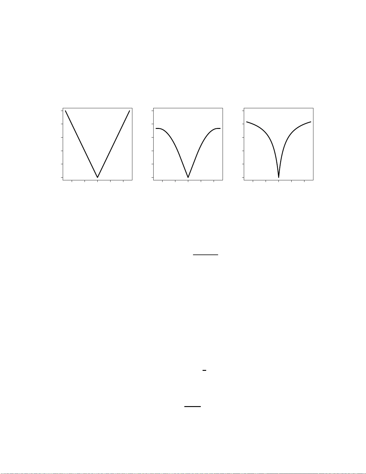
MM Algorithm s for Minimizing Nonsmoot hly Penalized Objecti ve Functions Elizabeth D. Schif ano ∗ , Robert L. Strawderman ∗ , Martin T . W ells ∗ Abstract The use of regular ization, or penalization , has become increasingly co mmon in high- dimensiona l statistical analysis over the past dec ade, wh ere a com mon g oal is to simultane ously select importan t variables and estimate their e ﬀ ects. It has been sho wn by se veral authors that these goals can b e achiev ed by minimizing some para meter-dependent “good ness of ﬁt” f unction (e.g., a negative log likelihood) subject to a penalizatio n tha t p romotes sparsity . Penalty f unctions that are nonsmo oth (i.e. not di ﬀ erentiable) at the or igin h av e rece i ved substantial attention, ar guably beginning with LASSO (T ibshirani, 1996). The current literature ten ds to f ocus on speciﬁc co mbination s of smo oth data ﬁd elity ( i.e., goodn ess-of-ﬁt) and non smooth penalty functions. One result of this combined speciﬁcity has been a proliferation in the number of computational algorithm s designed to solve f airly narrow classes of optimization prob lems in v olving objectiv e functions that are no t e verywhere continuously di ﬀ eren- tiable. I n this paper , we propose a general class of algorithms for optimizing an e xtensive v ariety of nonsmoo thly penalized objective functions that satisfy certain regularity co nditions. The proposed framework utilizes the majorization-min imization (MM) algorithm as its core optimization engine. The resulting alg orithms rely on iterated sof t-threshold ing, implemented c ompon entwise, allowing for fast, stable upd ating that av oids the n eed for any hig h-dimen sional matrix in version. W e establish a local co n vergence theor y for this class of algorith ms under weaker assump tions than previously considered in the statistical literature. W e a lso demonstrate the e xceptiona l e ﬀ ecti veness o f ne w ac- celeration methods, originally propo sed f or the EM alg orithm, in t his class of proble ms. Simulation results and a microarray d ata examp le are p rovided to demonstrate th e algo rithm’ s capabilities and versatility . K e ywor ds: Iterative Soft Thresholdin g, MIST , MM algo rithm. 1 Introd uction V ariable selecti on is an important and challen ging issue in the rapidly growing realm of high- dimensio nal statistical modeling. In such cases , it is often of interest to identify a few important v ariabl es in a ve ritable sea o f nois e. Modern metho ds, increa singly based on the principle of pena lized likel ihood estimatio n applied to high dimension al regressi on problems, attempt to ac hie v e this goa l thro ugh an adapti v e v ariabl e selection process tha t simultane ously permits estimation of reg ression e ﬀ ects. Indeed, the literatur e on the penalization o f a “goodness of ﬁt” function (e .g., ne gati v e loglik eliho od), with a penalt y singular at the origin, is quickly becoming va st, prolifera ting in part due to the considerati on of ∗ Department of Statistical Science, 301 Malott Hall, Cornell Univ ersity , Ithaca NY 14853 USA 1 speciﬁc combina tions of data ﬁdel ity (i.e., goodn ess-of- ﬁt) and pena lty fu nction s, the as sociat ed statis ti- cal p roperti es of resu lting estimato rs, and the dev elopmen t of se v eral c ombinati on-spe ciﬁc optimization algori thms, (e.g., Ti bshiran i, 1 996; Zou, 20 06; Zou and Hastie, 2005; Zou and Zhang, 2009; Fan and Li, 2001; Park and Hasti e, 2007; Friedman et al., 2008). In this pape r , we pr opose a uniﬁed opti mization framewo rk that appe als to the Majorizati on- Minimizati on (MM) algorith m (Lange, 2004) as the primary optimization tool. The resulting class of algorith ms is referred to as M IST , an acronym for Minimization by Iterati ve Soft Thresholdin g. The MM algorithm has been considered be fore f or solvin g speci ﬁc cl asses of singu larly pe nalized like lihood estimatio n proble ms (e.g., Daubechies et al., 2004; Hunter and Li, 2005; Zou and Li, 2008); to a large ext ent, this work is m oti v ated by thes e ideas. A distinct adv antage of the prop osed work is the ex cep- tional versatilit y of the class of MIST algori thms, their associated ease of i mplementat ion and numerical stabili ty , and the dev elopmen t of a ﬁxed point con ver gen ce theory that permits weak er a ssumptio ns than exi sting paper s in this ar ea. W e emphasize here t he focus of this pa per is on the dev elop ment of a stab le and versatile class of algorithms applicabl e to a wide vari ety of singularly penaliz ed estimation prob- lems. In parti cular , the co nsidera tion of asymptotic and oracle p ropert ies of estimators d eri ve d fro m particu lar co mbinatio ns of ﬁ delity and penalty functions , as well as methods for e ﬀ ecti v ely choosing associ ated penalty parameters, are not focal points of this paper . A compreh ensi v e treatment of these results may be found in Johnson et al. (2008), where asymptot ics and oracle prope rties for estimato rs deri v ed from a general class of penalize d estimati ng equations are dev elope d in some detail. The paper is or ganiz ed as follows. In Section 2, we introdu ce notation and provide su ﬃ cien t condi- tions for local c on ver gence of t he MM algorithm app lied to a lar ge c lass of data -ﬁdelity an d no n-smooth penalt y functions. In Section 3, w e present a specialize d versio n of this general algorithm, demon strat- ing in particular ho w the minimization step of the M M algorithm can be carried out using iterated soft-th reshol ding. In its m ost general form, iterated soft-thre sholdi ng is required at each minimization step; we further de monstrat e how to car ry ou t this minimization step in one iteration throug h a judici ous choice of majo rizatio n function. As a con seque nce, we present a simpliﬁed cla ss of iterati v e algorith ms that are applica ble to a wide class of singularl y penalized, generalized linear regress ion models. Simulation results are provid ed in Section 4, while an applicatio n in surviv al analysis to Di ﬀ use Lar ge B Cell L ymphoma express ion data (Rosenw ald et al., 2002 ) is presen ted in Section 5. W e con- clude with a discus sion in Section 6. Proofs and other rele vant results are colle cted in the Appendix. 2 MM algorithms f o r nonsmooth objectiv e functions Let ξ ( β ) denote a real-v alued objecti ve func tion to be minimized for β = ( β 1 , . . . , β p ) T in some con vex subset B of R p . Let ξ S U R ( β , α ) denote a real-v alued “surrogate ” objecti ve functio n, where α ∈ B . Deﬁne the minimizatio n map M ( α ) = ar g min β ∈B ξ S U R ( β , α ) . (1) Then, if ξ S U R ( β , α ) majorizes ξ ( β ) for each α , a generic MM algorith m for m inimizing ξ ( β ) takes the follo wing form (e.g., Lange, 2004): 1. Initial ize β (0) 2. For n ≥ 0, compute β ( n + 1) = M ( β ( n ) ) , iter ating until con ver gence. 2 Provid ed that the objec ti ve function, its s urrogat e and the mappi ng M ( · ) satisfy certain re gularity condi- tions, one can est ablish con ver gence of t his algorithm to a local or glo bal solutio n. L ange (2004, Ch. 10) de velops such a the ory as suming that the objecti ve fun ctions ξ ( β ) an d ξ S U R ( β , α ) are twice c ontinu ously di ﬀ erenti able. For problems that lack this degree of smoothn ess (e.g., all singu larly penalized regres- sion problems, includ ing lasso, T ibshirani (1996); adapti ve lasso , Zou (2006); and SC AD, Fan a nd Li (2001)), a more general theory of local con ver gence is required . One such theory is summarized in Appendi x A.1; related results for the EM algorithm m ay be found in W u (1983), Tseng (2004) and Chr ´ etien and Hero (2008). Let k · k denote the us ual Euclide an vecto r norm. Based on the theory summari zed in Appen dix A.1, we propos e a new and general class of algorith ms for minimizin g penalized objecti ve functions of the form ξ ( β ) = g ( β ) + p ( β ; λ ) + λε k β k 2 , λ > 0 , ε ≥ 0 (2) where g ( β ) and p ( β ; λ ) are respe cti vely data ﬁdelity (e.g., nega ti ve logli keli hood) and penalty functions that satisf y regula rity condition s to be delineated belo w . As will be shown later , the class of problems repres ented by (2) contains all of the p enalize d reg ression problems co m monly c onsidered in the current literat ure. It also cov ers numerous other problems by exp anding the class of permissible ﬁdelity and penalt y functions in a substanti al way . W e assume t hrough out that g ( β ) is c on ve x and c oerci ve fo r β ∈ B , wh ere B is a n open con vex subset of R p . W e further assume that p ( β ; λ ) = p X j = 1 ˜ p ( | β j | ; λ j ) , (3) where the vector λ = ( λ T 1 , . . . , λ T p ) T and λ j denote s the block of λ associa ted with β j . It is assumed that each λ j has dimensio n greater than or equal to one, that all blocks ha ve the same dimension, and that the λ j 1 = λ for each j ≥ 1. Evidently , the case where dim( λ j ) = 1 for j ≥ 1 simply correspo nds to the setting in which each coe ﬃ cien t is penalized in exac tly the same way; permitting the dimension of λ j to exceed one allo ws the penalty to depen d on additio nal parameter s (e.g., weights, such as in the case of the adapti ve lasso considered in Zou (2006)). W e are interested in problems with penalizat ion; therefo re, λ is assumed bounded and strictly positi ve througho ut this pape r . Sev eral speciﬁc examples will be discussed belo w . For any bounded θ w ith λ > 0 as the ﬁrst element, and the remainder of θ collec ting any additiona l parameters used to deﬁne the penalty , the scala r functi on ˜ p ( r ; θ ) is assumed to satisfy the follo wing condition : (P1) ˜ p ( r ; θ ) > 0 for r > 0; ˜ p (0; θ ) = 0; ˜ p ( r ; θ ) is a continuo usly di ﬀ erentiable conca ve function with ˜ p ′ ( r ; θ ) ≥ 0 for r > 0, and, ˜ p ′ (0 + ; θ ) ∈ [ M − 1 θ , M θ ] for some ﬁnite M θ > 0. Evidentl y , (P1) implies that ˜ p ′ ( r ; θ ) > 0 for r ∈ (0 , K θ ) , where K θ > 0 m ay be ﬁnite or inﬁnite. The combina tion o f the conca vity and nonne gativ e deri v ati ve c onditio ns thus imply that the penalty increases awa y from the origin , b ut with a decreasi ng rate of gro wth that may become zero. The case where (3 ) is identically zero for r > 0 is ruled out by the positi vity of the right deri vati ve at the origin imposed in (P1); similarly , the conc a vity assumption also rules out the possibi lity of a strictly con ve x penal ty term. Neither of these restricti ons is particu larly problematic . Our speciﬁc interest lies in the dev elopment of algori thms for estimation problems subject to a penalt y singul ar at the origin. W ere (3) absent, or 3 replac ed by a strictl y con ve x penalty term, the con vex ity of g ( β ) implies (2) can be minimized directly using any s uitable con ve x optimiz ation algorithm, such as that discuss ed in T heorem 3.2 belo w . Theorem 2.1 estab lishes local con ver gence of the indi cated class of MM algorithms for m inimizin g object i ve functions of the form (2). A proof is provid ed in Appendix A .2, where it is sho wn that condit ions imposed in the statement of the theorem are su ﬃ cient condi tions for the appli cation of the genera l M M local con ver gence theory summarized in Appendix A.1. Theor em 2 .1. Let g ( β ) be con ve x and coer cive and assume p ( β ; λ ) satisﬁes both (3) and conditi on (P1). Let h ( β , α ) ≥ 0 be a r eal-va lued, continuo us function of β and α that is conti nuousl y di ﬀ er entiable in β for each α and satisﬁes h ( β , α ) = 0 when β = α . Let q ( β , α ; λ ) = p X j = 1 ˜ q ( | β j | , | α j | ; λ j ) , (4) wher e ˜ q ( r , s ; θ ) = ˜ p ( s ; θ ) + ˜ p ′ ( s ; θ )( r − s ) for r , s ≥ 0 , and deﬁne ψ ( β , α ) = h ( β , α ) + q ( β , α ; λ ) − p ( β ; λ ) . Assume the set of stati onary points S for ξ ( β ) , β ∈ B is ﬁ nite and isolated. Then: (i) ξ ( β ) in (2) is locally Lipschit z continuous and coer cive; (ii) q ( β , α ; λ ) − p ( β ; λ ) is eith er iden tically zer o or non-ne gative for all β , α ; (iii) ξ S U R ( β , α ) ≡ ξ ( β ) + ψ ( β , α ) majorizes ξ ( β ) and the MM algorithm derived fr om ξ S U R ( β , α ) con- ver ges to a stationa ry point of ξ ( β ) if ξ S U R ( β , α ) is uniquely minimized in β for each α and at least one of h ( β , α ) or q ( β , α ; λ ) − p ( β ; λ ) is st rictly positive for each β , α . Conditio n (iii ) o f T heorem 2.1 establi shes co n ver gence under the a ssumptio n that ξ S U R ( β , α ) strictly majorize s ξ ( β ) and has a uniqu e m inimizer in β for each α . Such a unique ness condition is shown by V aida (2005) to ensure con ver gence of the E M and MM algorith m s to a stationary point under more restric ti ve di ﬀ erentiabil ity condition s. Importantly , the assumption of globally strict majorization is only a su ﬃ cient condi tion for con ver gence; this condi tion is only important insofa r as it guara ntees a strict decrease in the objecti ve function at eve ry iteration. As can be seen from the proo f, it is possib le to relax this condit ion to locally strict majoriza tion, in which ξ S U R ( β , α ) majorizes ξ ( β ) , with strict majoriza tion being necessary only in an open neighborh ood containing M ( α ). The use of the MM algorith m and selecti on of (4) are moti vated by the results Zou and Li (2008); we refer the reader to Remark 3.1 belo w for further comments in this directi on. The assumptions on g ( β ) clearly cover the case of the linear and canonically paramete rized generali zed linear m odels upon setting g ( β ) = − ℓ ( β ) , w here ℓ ( β ) denotes the correspon ding loglik elihood functio n. Estimation under the semiparametric Cox regressio n model (Cox, 1972) and accelerate d failur e time models are also cov ered upon setting g ( β ) to be either the negat i ve logarithm of the partial likelih ood function (e.g., Andersen et al., 1993, Thm VII.2.1) or the G ehan objecti ve function (e.g., Fygenson and Ritov, 1994; Johns on and Strawderman, 2009). The ass umption (P1) on the pe nalty funct ion cove rs a wide v ariety of pop ular and interesting exam- ples; see Figure 1 for illustra tion. For ex ample, the lasso (LAS; e.g., T ibshirani, 1996), adapti ve lasso (ALAS; e.g., Zou, 2006), elasti c net (EN; e.g., Zou and Hastie, 2005), and adapt i ve elastic net (AEN; 4 e.g., Zou and Zhang, 2009) penalties are all recov ered as special cases upon consid ering the combi- nation of (3) and the ridge-type penalty λε k β k 2 . Speciﬁcally , w ith λ j = ( λ, ω j ) T for ω j ≥ 0, taking ˜ p ( r ; λ j ) = λω j r in (3) gi ves L AS ( ω j = 1 , ǫ = 0) , ALA S ( ω j > 0 , ǫ = 0), E N ( ω j = 1 , ǫ > 0) and the AEN ( ω j > 0 , ǫ > 0) penalties. It is easy to see that selecting ˜ p ( r ; λ j ) = λω j r also implies the equali ty of (3) and (4), a result rele vant in both (ii) and (iii) of Theorem 2.1 abo ve. −4 −2 0 2 4 0 1 2 3 4 5 LASSO [ θ = λ =1] r p ~ ( lrl , θ ) −4 −2 0 2 4 0 1 2 3 4 5 SCAD [ θ =( λ ,a)=(1.25,3.7)] r p ~ ( lrl , θ ) −4 −2 0 2 4 0 1 2 3 4 5 Geman & Reynolds, 1992 [ θ =( λ , δ )=(5,1)] r p ~ ( lrl , θ ) Figure 1: Three examples of penalt ies satisfying (P1). The propos ed penalt y speciﬁcatio n also cov ers the smoothly clipped absolute devi ation (SC AD; e.g., Fan and Li, 2001) penalty upon setting ˜ p ( r ; λ j ) = ˜ p S ( r ; λ, a ) for each j ≥ 1, where ˜ p S ( r ; λ, a ) is deﬁned as the deﬁnite inte gral of ˜ p ′ S ( u ; λ, a ) = λ [ I ( u ≤ λ ) + ( a λ − u ) + ( a − 1) λ I ( u > λ )] (5) on the in terv al 0 ≤ u ≤ r and some ﬁxed value of a > 2 (e .g., a = 3 . 7). The resulti ng penalty functi on is contin uously di ﬀ erentiable and conca ve on r ∈ [0 , ∞ ). T he conc a vity of ˜ p S ( · ; λ, a ) on [0 , ∞ ) , combin ed with ˜ p S (0; λ, a ) = 0 and the fa ct that ˜ p ′ S (0 + ; λ, a ) is ﬁnite, implies ˜ p S ( r ; λ, a ) ≤ ˜ p S ( s ; λ, a ) + ˜ p ′ S ( s ; λ, a )( r − s ) (6) for eac h r , s ≥ 0, the bound ary cases for r = 0 and / or s = 0 follo w ing from Hiriart-Urru ty and Lemar ´ echal (1996, Remark 4.1.2, p. 21). In other words, ˜ p S ( r ; λ, a ) can be majorized by a linear funct ion of r . The lasso pe nalty , its v ariants, and SCAD hav e recei ved the greatest atten tion in th e lite rature. More recent ly , Zhang (2007) introduced the m inimax conca ve penalty (MC P), which similarly to SCAD is deﬁned in terms of its deriv ati ve. S peciﬁcall y , one takes ˜ p ( r ; λ j ) = ˜ p M ( r ; λ, a ) for each j ≥ 1 in (3), where ˜ p M ( r ; λ, a ) is deﬁned for a > 2 as the deﬁnite integ ral of ˜ p ′ M ( u ; λ, a ) =  λ − u a  + (7) on the interva l 0 ≤ u ≤ r and some ﬁxed value of a > 2 (e.g., a = 3 . 7 as in Fan et al., 2009b). Further exa mples of di ﬀ erentiab le conca ve penaltie s include ˜ p ( r ; λ j ) = ˜ p G ( r ; λ, δ ) for ˜ p G ( r ; λ, δ ) = λ δ r 1 + δ r , δ > 0 (8) 5 (e.g. Geman and Reynol ds, 1992; Nikolo va, 2000); and ˜ p ( r ; λ j ) = ˜ p Y ( r ; λ, δ ) for ˜ p Y ( r ; λ, δ ) = λ log( δ r + 1) , δ > 0; (9) (e.g. Antonia dis et al., 2009). These pen alties represent just a small sample of the set of possib le penal- ties satisfy ing (P 1) that one might reasonab ly conside r . Remark 2.2. The SCA D and MCP penalties ar e not strictl y concave and lead to surr ogate majoriz ers that fail to satisfy the globally strict majoriza tion condition in (iii) of Theor em 2.1 unless h ( β , α ) is strictl y positive whenever β , α ; see Remark 3.1 for furt her discussio n and also Theor em 3.4 below . 3 MIST : Minimization by It erated Soft Thr esholding 3.1 The MIST algorithm In genera l, the statistica l literature on penaliz ed estimation has propo sed optimizati on algorith ms tai- lored for s peciﬁc combina tions of ﬁ delity a nd penal ty functi ons. The cla ss of MM algorith m s sugge sted by Theore m 2.1 pro vides a ver y genera l and useful frame work for pr oposin g ne w algorithms, the ke y to which is a metho dology for solvin g the minimizatio n problem (1), a step re peated with eac h iterati on of the MM algo rithm. In this regard , it is helpful to note that the problem of minimizing ξ S U R ( β , α ) for a gi ven α is equ iv alent to m inimizing g ( β ) + λε k β k 2 2 + h ( β , α ) + p X j = 1 ˜ p ′ ( | α j | ; λ j ) | β j | (10) in β . In particu lar , if g ( β ) + λε k β k 2 + h ( β , α ) is stri ctly con ve x for each bound ed α , which clearly occ urs if both g ( β ) and h ( β , α ) are con ve x in β and at least one is strictly con vex, then (10) is also strictly con vex and the correspo nding m inimizati on problem has a unique solution. Remark 3.1. F or ε = h ( β , α ) = 0 and g ( β ) = − ℓ ( β ) for ℓ ( β ) = P n i = 1 ℓ i ( β ) with ℓ i ( β ) a twice continuou sly di ﬀ er entiable lo glikeliho od functio n, the majorizer used by the MM algorithm induced by the surr ogate functi on (10) corr esponds (up to sign) to the minorizer employed in the LLA algorithm of Zou and Li (2008), an impr ovement on the so-calle d L QA algo rithm pr oposed in Hunter and Li (2005). Z ou and Li (2008, Pr oposition 1) assert con ver gence of their LLA algorithm under impr ecisely stated assumptions and ar e addition ally unclear as to the natur e of con ver gence res ult actually estabi shed. F or e xample, while Zou and Li (2008, Theor em 1) demonstr ate that the LLA algorithm does indeed have an ascent pr operty , their re sult appears to be insu ﬃ cient to ensur e that the pr oper analo g of condi tion Z3(ii) of Theor em A. 1 hol ds in the case of the SCAD penalty . A s a conse quenc e, it is uncle ar whether even weak “subsequ ence” con ver gen ce r esults (cf. W u, 1983) hold with useful gener ality in the case of the LLA algori thm. In contrast, Theor em 2.1 shows that strict m ajoriz ation, under a few pr ecisely stated condi- tions, is su ﬃ cien t to ensur e loc al con ver gence of the r esulting MM algorithm to a sta tionary point of (2) In Sectio n 3.2 , it is fu rther de monstr ated how a particular ch oice of h ( β , α ) yields a strict maj orizer t hat permits both clos ed form minimization and componen twise updating at each step of the MM alg orithm, eve n in the case of penalties that fail to be strictly concave . Numerous methods exist for minimizing a di ﬀ ere ntiable con ve x obje cti ve function (e.g., Boyd and V ande nber ghe , 200 4 ). Howe ver , bec ause (10) is not di ﬀ ere ntiable , such method s do n ot apply 6 in the curren t setting. Special ized methods exis t for nonsmoo th problems of the form (10) in setting s where g ( β ) has a speci al structure; a well-kno w n example here is LARS (Efron et al., 2004), which can be us ed to e ﬃ ci ently solv e lasso-type problems in th e case where g ( β ) i s replac ed by a l east square s ob- jecti ve functio n. Rece ntly , Combettes and W ajs (2005, Proposit ion 3.1; Theorem 3.4) proposed a ve ry genera l class of ﬁ xed point algorit hms for minimizi ng f 1 ( h ) + f 2 ( h ) , where f i ( · ) , i = 1 , 2 are ea ch con vex and h takes valu es in some real Hilbert space H . Hale et al. (2008, Theo rem 4.5) specia lize t he results of Combettes and W ajs (2005) to th e cas e where H is so me sub set of R p and f 2 ( h ) = P p j = 1 | h i | . The coll ec- ti ve applicatio n of these results t o the problem of minimizing (10) generates an iterated soft-t hresho lding proced ure with an appealingly simple structure. Theorem 3.2, giv en belo w , states the algorithm, along with conditions under w hich the algo rithm is guaran teed to con ver ge; a proof is provid ed in Appendix A.3. The resul ting class of procedures , that is, MM algorithms in which t he mini mization of (10) is car - ried out via this iterated soft-t hresho lding procedu re, is hereafter referr ed to as MIST , an acron ym for (M)inimiza tion by (I)terated (S)oft (T)hresh olding . T wo import ant and useful featu res of MIST includ e the absence of high-di mensiona l matrix in version and the ability to update each indi vidual parameter separa tely . Theor em 3.2. Supp ose the conditio ns of Theor em 2.1 hold. Let m ( β ) = g ( β ) + h ( β , α ) + λǫ k β k 2 be strictl y con vex w ith a Lipsch itz continuo us derivati ve of or der L − 1 > 0 for eac h bounded α . Then, for any suc h α and a constant  ∈ (0 , 2 L ) , the unique minimizer of (10) can be obta ined in a ﬁnit e number of iter ations using iterated soft-th r esholding : 1. Set n = 1 and initia lize b (0) 2. Compute d ( n ) = b ( n − 1) −  ∇ m ( b ( n − 1) ) 3. Compute b ( n ) = S ( d ( n ) ;  τ ) , wher e for any vectors u , v ∈ R p , S ( u ; v ) = p X j = 1 s ( u j , v j ) e j , (11) e j denote s the j th unit vector for R p , s ( u j , v j ) = sign ( u j )( | u j | − v j ) + , (12) is the univa riate soft-thr eshold ing operat or , and τ = ( ˜ p ′ ( | α 1 | ; λ 1 ) , . . . , ˜ p ′ ( | α p | ; λ p )) T . 4. Stop if con ver ged ; else , set n = n + 1 and r eturn to Step 2. The pro posed algo rithm, as orig inally de veloped in Combett es and W ajs (20 05), is sui table for min - imizing the sum of a di ﬀ erentiable con ve x function m ( · ) and another con ve x function; hence, under similar conditio ns, one could employ this algorithm directly to minimize (2) in cases w here the penalt y (3) is deri ved from some con ve x function ˜ p ( · ; θ ). Theorem 3.4 of Combettes and W ajs (2005) further sho ws that the update in Step 3 can be generaliz ed to b ( n ) = b ( n − 1) + δ n h S  b ( n − 1) −  n ∇ m ( b ( n − 1) );  n τ  − b ( n − 1) i , 7 where, for e very n ,  n ∈ (0 , 2 L ) and δ n ∈ (0 , 1] is a suitable seque nce of relaxation constan ts. Judicio us selecti on of these constan ts, possibly updated at each step, m ay impro ve the con ver gence rate of this algori thm. Theorem 3.2 imposes the relati vely strong condition that the gradient of m ( β ) is L − 1 -Lipschit z con- tinuou s. The role of this condition, also imposed in Combettes and W ajs (200 5, Propositio n 3.1; The- orem 3.4), is to ensur e that the update at each step of the propo sed algor ithm is a contracti on, thereby guaran teeing its con ver gence to a ﬁxed point. T o see this, note that the update from b ( n ) to b ( n + 1) in the algori thm of Theorem 3.2 in volv es the mapping S ( b −  ∇ m ( b );  τ ) . For any bounded b and a , it is easily sho wn that k S ( b −  ∇ m ( b );  τ ) − S ( a −  ∇ m ( a );  τ ) k ≤ k b − a −  ( ∇ m ( b ) − ∇ m ( a ) ) k . When ∇ m ( b ) = ∇ m ( a ), the r ight-ha nd side reduce s to k b − a k , and the resultin g m apping is on ly nonex- pansi ve (i.e., not necessa rily contracti ve). Howe ver , under strict con ve xity , this situatio n can occur only if b = a . In partic ular , suppose that b ( n ) , b ( n − 1) ; t hen, ∇ m ( b ( n ) ) , ∇ m ( b ( n − 1) ) a nd, us ing th e mean v alue theore m, k b ( n + 1) − b ( n ) k = k S  b ( n ) −  ∇ m ( b ( n ) );  τ  − S  b ( n − 1) −  ∇ m ( b ( n − 1) );  τ  k ≤ k I −  H ( b ( n ) , b ( n − 1) ) k k b ( n ) − b ( n − 1) k , where H ( b , a ) = R 1 0 ∇ m ( b + t ( a − b )) d t . T he assumption that the gradien t of m ( β ) is L − 1 -Lipschit z contin uous now implies that choosing  as indicated guaran tees k I −  H ( b ( n ) , b ( n − 1) ) k < 1, thereby produ cing a contraction . In view of the general ity of the Contractio n Mapping T heorem (e.g., Luenber ger and Y e, 2008, Thm. 10.2.1), it is possib le to relax the requirement that ∇ m ( β ) is globally L − 1 -Lipschit z continuou s pro vided that one selects a suitable startin g point . The rele v ant ex tension is summariz ed in t he co rollary belo w; one may prov e this result in a m anner similar to Theorem 4.5 of Hale et al. (20 08). Cor ollary 3.3. Let the con ditions of Theor em 2.1 hold . Suppo se α is a boun ded vector and ass ume that m ( β ) = g ( β ) + h ( β , α ) + λǫ k β k 2 is strictl y con vex an d twice continuo usly di ﬀ er entiable . Then, fo r a given bound ed α , ther e exists a uniqu e minimizer β ∗ . Let Ω be a boun ded con ve x set con tainin g β ∗ and deﬁ ne λ ma x ( β ) to be the lar ges t eige n value of ∇ 2 m ( β ) . Then, the algo rithm of T heor em 3.2 con ver ges to β ∗ in a ﬁnite number of itera tions pr ovided that b (0) ∈ Ω , λ ∗ = max β ∈ Ω λ ma x ( β ) < ∞ , an d  ∈ (0 , 2 /λ ∗ ) . Some useful insight into the form of the proposed thresholdin g algorit hm can be gained by consid- ering the beha vior of the penalty deriv ati ve term ˜ p ′ ( r ; θ ) . As sugges ted earlier , (P1) implies that ˜ p ′ ( r ; θ ) decrea ses from its m aximum value towa rds zero as r mov es away from the origin. For some penal- ties (e.g., SCAD, MCP ), this deri vati ve actually becomes zero at some ﬁnite val ue of r > 0, resultin g in situations for which τ j = ˜ p ′ ( | α j | ; λ j ) = 0 for at least one j . If this occurs for componen t j , then j th compone nt of the vector S  b ( n ) −  ∇ m ( b ( n ) );  τ  simply reduces to the j th compone nt of the ar- gument vecto r b ( n ) −  ∇ m ( b ( n ) ). In the extreme case where τ = 0 , the proposed update reduce s to b ( n + 1) = b ( n ) −  ∇ m ( b ( n ) ) , an inexact Newton step in which the in verse hessian matrix is replaced by  I p , I p denoti ng the p × p identity m atrix, and with step- size chosen to ensure that this update yields a contra ction. Hence, if each of the components of b ( n ) −  ∇ m ( b ( n ) ) are su ﬃ cie ntly larg e in magnitud e, the proposed algorithm simply takes an inexac t Newton step tow ards the solution; otherwise, one or more componen ts of this Newton- like update are subject to soft-thr eshold ing. 8 3.2 Pe nalized estimation for gen eralized linear models The combinatio n of Theorems 2.1, 3.2 and Corollary 3.3 lead to a useful and stable class of algorithms with the ability to deal with a wide range of penalized regressio n problems. In settings where g ( β ) is strictl y con ve x and twice continu ously di ﬀ erentiable , one can safely assume that h ( β , α ) = 0 for all choice s of β and α provide d that ˜ p ′ ( r ; θ ) in (P1) i s stri ctly positi ve for r > 0; importan t exa mples of sta - tistica l estimation problems here include many commonly used linear and general ized linear regressio n models, semiparametri c Cox reg ression (Cox, 1972), and smoothed ve rsions of the accele rated failure time regre ssion model (cf. Joh nson and Strawderman, 2009). The SCAD and MCP penali zation s, as well as other penalties ha ving ˜ p ′ ( r ; θ ) ≥ 0 for r > 0 , can also be used; ho weve r , additional care is requir ed. In particular , and as point ed out in an earlier remark, if one sets h ( β , α ) = 0 for all β and α then con ver gence of the resul ting algorithm to a stationa ry point is no longer guaran teed by the abov e results due to the resul ting failure of these penalties to induce strict majorization . The need to use an iterati ve algorit hm for repeatedly minimizing (10) is not unusu al for the class of MM algorith ms. Ho w e ver , it turns out that for certain choices of g ( β ), a suitable choice of h ( β , α ) in Theorem 3.2 guarantees both strict majorization and permits one to minimize (10) in a single iter- ation, resulti ng in a single soft-thresh olding update at each iteration. Belo w , we demonstrate how the MIST algorithm simpliﬁes in settin gs where g ( β ) correspond s to th e ne gativ e logl ike lihood func tion of a canon ically parameterize d genera lized linea r regres sion m odel ha ving a bounded hessian function. The result applies to all pena lties satisfying condition (P1), inclu ding SC AD and MCP . A proof is provided in Append ix A.4. Theor em 3.4. Let y be N × 1 and suppose the pr obabilit y distrib ution of y follows a gen eral ized linear model w ith a cano nical link and linear pr edicto r e X e β , wher e e X = [ 1 N , X ] is N × ( p + 1) an d e β = [ β 0 , β T ] T is ( p + 1) × 1 with β 0 denoti ng an inter cept. Assume that g ( e β ) = − ℓ ( e β ) , wher e ℓ ( e β ) = 1 T ( c ( y ) − b ( e η )) + y T e η denote s the corr espon ding loglik elihood; her e, e η = e X e β and E [ y i ] = b ′ ( ˜ η i ) for i = 1 . . . N for b ( · ) strict ly con vex and twice conti nuousl y di ﬀ er entiable . L et the penalty function be deﬁned as in (3) and satis fy (P1); note that β 0 r emains unpenalize d. Deﬁne h ( e β , e α ) = ℓ ( e β ) − ℓ ( e α ) − ∇ ℓ ( e α ) T ( e β − e α ) +  − 1 ( e β − e α ) T ( e β − e α ); (13) wher e ˜ α ≡ [ α 0 , α T ] T is ( p + 1) × 1 , and  is deﬁne d as in C or ollary 3.3 . Then: 1. The object ive function (2) , say ξ glm ( ˜ β ) , is major ized by ξ S U R glm ( ˜ β , ˜ α ) = − ℓ ( ˜ α ) − ∇ ℓ ( ˜ α ) T ( ˜ β − ˜ α ) +  − 1 ( ˜ β − ˜ α ) T ( ˜ β − ˜ α ) + p X j = 1 ( τ j | β j | + γ j + λǫ β 2 j ) (14) wher e τ j = ˜ p ′ ( | α j | ; λ j ) and γ j = ˜ p ( | α j | ; λ j ) − ˜ p ′ ( | α j | ; λ j ) | α j | ar e bou nded, nonne gative , and func- tional ly independe nt of ˜ β . 2. The functi ons g ( e β ) = − ℓ ( ˜ β ) and h ( ˜ β , ˜ α ) satisfy the r e gularit y conditions of Theor ems 2.1 and 3.2; hence , the corr espon ding MM algorithm con ver ges to a stationary point of (2) . 9 3. F or each bou nded ˜ α , (a) the minimizer ˜ β ∗ of ξ S U R glm ( ˜ β , ˜ α ) is unique and satisﬁe s β ∗ = 1 1 + λǫ S  α +  2 [ ∇ ℓ ( ˜ α )] A ,  2 τ  , β ∗ 0 = α 0 +  2 [ ∇ ℓ ( e α )] 0 (15) wher e S ( · ; · ) is the soft-th resh olding operator deﬁne d in (11) and A = { 1 , . . . , p } . (b) for each ˜ κ ≡ [ κ 0 , κ T ] T ∈ R ( p + 1) , ξ S U R glm ( ˜ β ∗ + ˜ κ , ˜ α ) ≥ ξ S U R glm ( ˜ β ∗ , ˜ α ) +  − 1 k ˜ κ k 2 . (16) In vie w of previo us results, the result in # 3 of Theorem 3.4 shows that the resultin g MM algorith m tak es a very simple form: giv en the current iterate e β ( n ) , 1. update the unpen alized intercept β ( n ) 0 : β ( n + 1) 0 = β ( n ) 0 +  2  ∇ ℓ ( ˜ β ( n ) )  0 2. update the remainin g parameters β ( n ) : β ( n + 1) = 1 1 + λǫ S  β ( n ) +  2 [ ∇ ℓ ( ˜ β ( n ) )] A ;  2 τ ( n )  , (17) where τ ( n ) = ( ˜ p ′ ( | β ( n ) 1 | ; λ 1 ) , . . . , ˜ p ′ ( | β ( n ) p | ; λ p )) T . The speciﬁc choice of functio n h ( e β , e α ) clear ly serves two useful purpos es: (i) it leads to compone ntwise-so ft thresholdi ng; and, (ii) it leads to strict majorizatio n, as is required in condition (iii) of Theore m 2.1, allo wing one to establish the con ver gence of MIST for SC AD and other penalties ha ving ˜ p ′ ( r , θ ) = 0 at some ﬁnite r > 0 . Evidentl y , the algori thm abov e immediately cov ers the setting of penal ized linear regress ion. For exa mple, suppose that y has been center ed to remov e β 0 from considerat ion and that the problem has also been resca led so that X , which is no w N × p , satisﬁes the indicat ed condition s. T hen, the resu lts of the Theorem 3.4 apply directl y w ith − ℓ ( β ) = 1 2 k X β − y k 2 , ∇ ℓ ( β ) = X T ( y − X β ) , h ( β , α ) =  − 1 k β − α k 2 − 1 2 k X β − X α k 2 , where  is deﬁned as in Corolla ry 3.3. For the class of adapti ve elastic net penalties (i.e., ˜ p ( r ; λ j ) = λω j r in (3)), the resulting iterati ve scheme is exactly that proposed in (De Mol et al., 2008, pg. 17), specialized to th e sett ing of a Euclidean paramete r . In part icular , we ha ve τ j = λω j and γ j = 0 in Theorem 3.4, and the propos ed update reduces to β ( k + 1) = 1 ν + 2 λǫ S  ( ν I − X ′ X ) β ( k ) + X ′ y ; λ  , where ν = 2  − 1 . Setting ν = 1 and ǫ = 0 yields the iterati ve procedure proposed in Daubechi es et al. (2004), p rov ided tha t X ′ X is sc aled such tha t I − X ′ X is posit iv e deﬁnite. The prop osed MIST algorithm 10 ext ends these iterati ve compone ntwise soft-thres holdin g procedures to a m uch wider class of penalty and data ﬁdelity functio ns. The restriction to canoni cal generali zed linear m odels in T heorem 3.4 is imposed to ensure strict con vexit y of the negati ve loglik elihoo d. Our results are easily modiﬁed to handle non-canon ical gener - alized linear models, provide d the neg ativ e loglik elihood remains strictly con vex in e β and the hessia n can be appropria tely bounded. Interes tingly , not all canon ically paramet erized general ized linear m od- els satisfy the regular ity condition s of Theore m 3.4. One such important class of problems is penalized like lihood estimatio n for Poi sson reg ression models. For example, in the classical setting of N indepen- dent Poisson observ ations with E [ Y i | ˜ X i ] = d i exp { ˜ x T i e β } for a known set of constan ts d 1 . . . d N , we ha ve (i.e., up to irrele van t const ants) ℓ ( e β ) = − P N i = 1 f i ( ˜ x T i e β ) , where f i ( u ) = d i e u − y i u . It is easy to see that ∇ ℓ ( e β ) , hence ∇ m ( e β ) , is locally but not globally Lipschitz continuou s; hence, it is not possib le to choo se a matrix C =  − 1 I such that (14) ev erywhere majorizes ξ glm ( e β ). Ne verth eless, progre ss remains possible. For e xample, Corollary 3.3 implies that tha t one can still use a s ingle update of the form (17) prov ided that a suitable Ω , hence C and e β (0) , can be identiﬁed. Alternati vely , using results summarized in Becker et al. (19 97 ), one can instead majorize − ℓ ( e β ) for any boun ded α using k ( e β , e α ) = p X j = 0 k j ( β j ; α j ) for k j ( β j ; α j ) = n X i = 1 I { x i j , 0 } θ i j f i x i j θ i j ( β j − α j ) + ˜ x T i e α ! , where, for ev ery i , θ i j ≥ 0 are any sequence of constants satisfyin g P p j = 0 θ i j = 1 and θ i j > 0 if x i j , 0 . Of importance here is the fac t k j ( β j ; α j ) is a strict ly con vex function of β j and does not depen d on β k for k , j . O ne may now take h ( e β , e α ) in Theorem 2.1 as being equal to k ( e β , e α ) + ℓ ( e β ) , leadin g to the minimizatio n of ξ S U R ( e β , e α ) ∝ p X j = 1 [ k j ( β j ; α j ) + λεβ 2 j + ˜ p ′ ( | α j | ; λ j ) | β j | ] + k 0 ( β 0 , α 0 ) . (18) In pa rticula r , componentwise soft-th reshold ing is replaced by c omponen twise minimization of (18), the latter bein g possible using any algo rithm capable of minimizing a continu ous nonlinea r function of one v ariable. Remark 3.5. The Cox pr oportiona l hazar ds model (Cox, 1972), while not a gener alized linear model, shar es the essential featur es of the genera lized linear m odel utilized in Theor em 3.4. In partic ular , the ne gative log partia l likel ihood, say g ( β ) = − ℓ p ( β ) , is strictly con vex, twice continuous ly di ﬀ er entiable, and has a bounded hessian (e.g . , Bohning and Lindsay, 1988; A nder sen et al., 1993). Consequ ently , Theor em 3.4 and its pr oof are easily modiﬁed for this setting upon taking g ( β ) as indicat ed, setting h ( β , α ) = ℓ p ( β ) − ℓ p ( α ) − ∇ ℓ p ( α ) T ( β − α ) +  − 1 k β − α k 2 , and taki ng  as deﬁned as in Cor ollary 3.3. 3.3 Accelerating Con vergenc e Similarly to the EM algorithm, th e stability and simplicity of the MM algorit hm frequentl y comes at the price of a slow con ver gence rate. Numerous methods of acceler ating the EM algorithm ha ve been pro posed in the literature; see McLachlan and Krishnan (2008) fo r a rev ie w . Recently , 11 V aradha n and R oland (2008) proposed a new m ethod for EM called SQU AREM, obtained by “squari ng” an itera ti ve Ste ﬀ ensen- type (ST EM) acceleratio n method. B oth S TEM and S QU AREM are structure d for use with iterati ve mappings of the form θ n + 1 = M ( θ n ) , n = 0 , 1 , 2 , . . . , hence applicable to both the EM and MM algor ithms. Speciﬁcally , the accelerat ion update for SQU AR EM i s giv en by θ n + 1 = θ n − 2 γ n ( M ( θ n ) − θ n ) + γ 2 n [ M ( M ( θ n )) − 2 M ( θ n ) + θ n ] = θ n − 2 γ n r n + γ 2 n v n , (19) where r n = M ( θ n ) − θ n and v n = ( M ( M ( θ n )) − M ( θ n )) − r n for an adap ti ve ste plength γ n . V aradha n and R oland (2008) sugg est se ver al steple ngth options, with preferen ce for choice γ n = −k r n k / k v n k . Roland and V aradhan (2005) pro vide a proof of local con ver gence for SQU A REM under restric ti ve cond itions on the EM mappin g M ( θ ), while V aradhan and Roland (2008 ) outline a proo f for global con ver gence for version s of SQU AREM that employ a back-t racking strategy . W e study the e ﬀ ecti veness of SQU AREM applie d to the simpliﬁed form of the MIST algorithm, hereafte r denoted SQU AREM 2 , in Section 4.3. 4 Simulation Results The simulatio n results summarized belo w are intended to compare the estimates of β obtained from exi sting m ethods to those obtained using the simpliﬁed M IST algorithm of T heorem 3.4. In partic- ular , we consider the performance of MIST for the class of penalize d linear and generali zed linear models, demonst rating its capability of reco vering the solut ions provided by existi ng algorithms when both algorith ms are forced to use the same set of “tunin g” paramete rs (i.e., penal ty parameter (s), plus any additional parameters required to deﬁne the penalty itself). In cases w here multiple local minima can arise, we further show that the MIST algori thm often tends to ﬁnd solutions with lower objecti ve functi on ev aluations in comp arison with e xisting algorithms, prov ided these algo rithms utilize the s ame choice of starti ng valu e. 4.1 Example 1: Linear Model Let 1 m and 0 m respec ti vel y denot e m -dimen sional vect ors of ones and zeros. T hen, fol lo w ing Zou and Zhang (2009), we generat ed data from the linear regress ion m odel y = x ′ β ∗ + ε (20) where β ∗ = (3 · 1 T q , 0 T p − q ) T is a p -dimension al vec tor with intrinsic dimensio n q = 3[ p / 9] , ε ∼ N (0 , σ 2 ) , and x follo ws a p -dimen sional multi varia te normal distri b ution with zero mean and cov ariance matrix Σ ha ving elemen ts Σ j , k = ρ | j − k | , 1 ≤ k , j ≤ p . W e consi dered σ ∈ { 1 , 3 } , ρ ∈ { 0 . 0 , 0 . 5 , 0 . 75 } and p ∈ { 35 , 81 } for N = 100 independe nt obse rv ations. Penalized least squares estimation is considere d for ﬁve popula r choices of penalty functions, all of which are curre ntly implemented in the R so ftware languag e (R Dev elopment Core T eam, 2005): LAS, ALAS, EN, A EN, and S CAD. T he LA S, AL AS, EN and AEN penalti es are all con vex and lead to uniqu e solutions under mild conditions; the SCAD penalt y is conca ve and the result ing minimization proble m may hav e multiple solutions . In each case, we used existing software for computing solu tions subjec t to these penaliza tions and compared those results to the solution s computed using the MIST algori thm. 12 Regar ding existi ng methods, we respecti vely used the lar s (Hastie and Efron, 2007) and elasticn et (Zou and Hastie, 2008) packages for computing soluti ons in the case of the LA S and EN penalti es. For the ALAS a nd AEN penalties, we used so ftware kindly provided by Z ou and Zhang (2009) that also makes use of the elasticnet pack age. The weights for the AEN penalty are computed using ω j = | ˆ β E N j | − γ , j = 1 , . . . , p , where ˆ β E N is an EN estimato r and γ is a positi ve constant. U sing EN -based weights in the AE N ﬁtting algorith m n ecessitates tuning paramete r speciﬁcatio n for both EN and AEN . As in Zou and Zhang (2009), the ℓ 1 paramete rs λ ( λ 1 in their notation) are allowed to di ﬀ er , whereas the ℓ 2 paramete rs ǫ ( λ 2 in their notation) are forced to be the same. Evidentl y , setting ǫ = 0 ( λ 2 = 0) result s in the ALAS solution. F or the SCAD penalty , we considered the estimato r of Kim et al. (2008) (HD), as well the one-step SCAD (1S) and L LA estimators of Z ou and Li (2008). The code for the ﬁrst two methods was kindly provid ed by their respecti ve authors; the LL A estimator was computed using the R pa ckage SIS . The choice a = 3 . 7 was used for all implemen tations of SCA D. W e considered ﬁnding solu tions using penal ties in the set Λ = { 0 . 1 , 1 , 5 , 10 , 20 , 100 } . In particular , for L AS and SC AD, λ = λ 1 ∈ Λ . For E N, both λ = λ 1 ∈ Λ and λǫ = λ 2 ∈ Λ . For simplicity , w e ﬁxed the weigh ts for AEN for a gi ven λ 2 by selec ting the ‘be st’ ˆ β E N among the s ix estimat ors in v olving λ = λ 1 ∈ Λ based on a BIC-like criteria . Like wise for AL AS, the weights were computing using the ‘best’ ˆ β LA S among the six estimato rs in vo lving λ = λ 1 ∈ Λ . The parameter γ for the ALAS and AEN penalt ies was respec ti vely set to three and ﬁve f or p = 35 and p = 81. For the stri ctly con ve x objecti ve functio ns associat ed with th e LAS , ALA S, E N, and AEN penalties, we simply used a startin g v alue of β (0) = 0 p . For SC AD, three di ﬀ erent starting values for the MIST , HD, and L LA S CAD algorithms were consid ered: β (0) = 0 p , β (0) = b β ml (i.e., the unpenalized least squa res estimate) , and β (0) = b β 1 S ,λ (i.e., the one-step estimate computed using the penalty λ ). As in Zou and Li (2008), the one-ste p estimator 1S is computed using b β ml , an approp riate choice when N > p . The con ver gence criteria used by t he e xisting softw are packages were used without altera tion in th is simulatio n study . T he con ver gence criteria used for MIS T were as follows: the algorit hm stopped if either (i) the normed di ﬀ erenc e of successi ve iterates was less than 10 − 6 (con ver gence of coe ﬃ ci ents); or , (ii) the d i ﬀ erence of the o bjectiv e function e valu ated at succe ssi ve iterates wa s l ess th an 10 − 6 and t he number of iterati ons exce eded 10 6 (con ver gence of optimization) . Due to the lar ge number of compar - isons and h ighly inten si ve nature of the c omputati ons, we ran B = 100 simul ations for each ch oice of ρ , σ , and p . W e report the results for the con ve x penalties in T able 1 and those for the SCAD penalty in T ables 2 and 3. In T able 1, we s umm arize the a verag e normed di ﬀ erence between the sol ution obtained using exi st- ing soft ware and tha t obtain ed using MIST ,    ˆ β e xi st − ˆ β mi st    , over the B = 100 simulat ions; in particular , we report in the two leftmos t panels the maximum valu e of this di ﬀ erence , computed across all com- binati ons of tuning parameters. These maximum di ﬀ erences (all of w hich are multiplied by 10 5 ) are remarkab ly small for all (A)LAS and (A)EN penalt ies, indicatin g that MIST rec overs th e s ame (unique) soluti ons as the existin g algorit hms. Interes tingly , the valu es for LAS are slightly larg er than the rest, where the maximum di ﬀ erences all resulted from the smallest val ue of λ considered ( λ = 0 . 1). In these cases, the algorithm tended to stop using the objecti ve function criteria rather than the (stricter) coe ﬃ cie nt criteria, resulting in slightly large r di ﬀ erences on av erage. The results for S CAD are reported in T ables 2 ( p = 35) and 3 ( p = 81) and display (i) the av erage normed di ﬀ erences, multip lied by 10 3 , for ea ch combina tion of λ , ρ , σ , p and st arting v alue; a nd, (ii) the propo rtion of simulated datasets in which the MIST solutio n yields a lower ev aluation of the obje cti ve functi on in comparis on with the solution obtained using another method for the indicated choice of 13 T able 1: Maximum average normed di ﬀ erences ( × 1 0 5 ) over B = 100 simulations f or E xamples 1 (LM) and 2 (GLM). L M : σ = 1 L M : σ = 3 G L M ρ 0 0.5 0.75 0 0.5 0.75 0 0.5 0.75 p = 35 q = 25 LAS 0.10 0.35 1.45 0.10 0.37 1.56 0.07 4.28 6.17 ALAS 0.03 0.14 0.64 0.05 0.21 1.00 1.84 2.86 3.76 EN 0.07 0.19 0.50 0.07 0.20 0.51 2.30 5.61 8.68 AEN 0.03 0.10 0.33 0.04 0.13 0.36 1.47 3.35 5.27 p = 81 q = 75 LAS 1.73 3.82 11.76 2.33 5.78 18.99 0.10 6.97 9.94 ALAS 0.12 0.38 1.58 0.35 1.03 4.39 1.34 2.55 3.30 EN 0.31 0.49 0.87 0.31 0.49 0.88 2.35 4.64 6.56 AEN 0.14 0.22 0.56 0.16 0.26 0.56 1.27 2.29 2.85 startin g value. The results for λ = 100 are not s hown, as the solu tion was 0 p in all cas es. In comparis on with the con ve x penalti es, larger normed di ﬀ erences are obse rved, eve n when controlling for the use of the same starting va lue. Such di ﬀ erenc es are a result of two importan t features of the SC AD optimization proble m: (i) the possible exis tence of se veral local minima; and, (ii) the fact that the MIST , HD, and LLA algorithms each take a di ﬀ erent path from a giv en starting v alue tow ards one of these soluti ons. For example, while each of the LLA, MIST , and HD algorith m s in vol ve majorization of the objecti ve functi on using a lasso-type surrogate objecti ve functio n, both the majorization and minimization of the resulti ng surrogate functio n are carried out di ﬀ eren tly in each case . In partic ular , the LLA alg orithm, as implemente d in SIS , m ajorize s only the penalty term and adapt s the lasso code in glmpath in order to minimize the correspo nding surrogat e objecti ve function at each step. The HD algorithm is similar in spirit, b ut inst ead deco mposes the penalty term into a sum of a conca ve and con ve x functio n and ut ilizes the t he alg orithm of R osset and Zhu (2 007) to m inimize th e cor respon ding surrogate objec ti ve fu nction . The MIST alg orithm instead uses the same p enalty majorizat ion as the LLA algo rithm, bu t additiona lly majorize s the negati ve loglike lihood term in a way that permits minimizati on of the surrog ate functio n in a single soft-t hresho lding step. E ach procedure therefo re takes a di ﬀ erent path tow ards a solution, e ven when g iv en the same starting value . W e remark here that di ﬀ erences must also expec ted between any of LLA, HD, MIST and the one- step solution 1S; from a n opt imization per specti ve, the one-step es timate is the re sult of runn ing just one iterati on of the LLA algori thm, starting from the unpenal ized least squares estimator b β ml (Zou and Li, 2008), and only provid es an approximat ion the solution to the desired minimization problem. All other methods (L LA, MIST , HD) iterate until some local minimizer (or stationary point) is reached. For ex- ample, whe n usin g either b β ml or b β 1 S ,λ as th e star ting v alue, MIST al ways found a solut ion that prod uced a lo wer ev aluation of the obje cti ve function in comparison to b β 1 S ,λ . Howe ver , when using the nu ll start- ing v alue of 0 p , th e o ne-ste p estimator did occasionall y result in a lower object i ve fu nction e valu ation in cases in vol ving smaller values of λ . This beha vior is not terri bly surprising; with small λ, the one-step soluti on should genera lly be close to the unpen alized least squares solution, as the objecti ve function itself is like ly to be dominated by the least squares term. Of all the SC AD algorithms consid ered here, MIST and LLA tended to ﬁnd the m ost similar solu - 14 tions (i.e., hav e the smallest normed di ﬀ erence s). For the cases in which the LLA solut ion had lower object i ve funct ion ev aluatio ns, all of th e MIST solutions were a lso LLA solutio ns; i.e, when st arting the LLA algor ithm with the MIST solut ion, the algorith m terminated at the startin g value (i.e., th e LLA so- lution coincides with the MIST solution). Wit h the exception of three of these cases, starting the MIST algori thm wit h the LLA solution also resulte d in the s ame beha vior . For the m ost part, the HD and MIST algori thms also gav e similar results, with one source of di ﬀ erence being the respecti ve stopping criteria used. The stopp ing criteria for HD, asses sed in order , are as foll o w s: (1) ‘con ver gence of optimizatio n’: stop if the absolute valu e of the di ﬀ erenc e of the objecti ve e valuat ed at success iv e iterates is less than 1e-6; (2) ‘con ver gence of penalty gradien t’: stop if the sum of the absolute value of the di ﬀ erences of the deri vati ve of the centered penalty ev aluated at successi ve iterates is less than 1e-6, (3) ‘con ver gence of co e ﬃ cient s:’ stop if the su m of t he absol ute valu e of th e di ﬀ erence s of succe ssiv e iterate s is less th an 1e-6, and (4) ‘jump-ov er’ criteria: stop if th e objecti ve at the p re vious iterate plus 1 e-6 was l ess than t he object i ve at the current iterate. After caref ul analysis of the results, we can assert the follo wing: • The MIST solution usually has the same or a lower ev aluation of the object i ve funct ion in com- pariso n w ith HD, re gardles s of starting v alue. • HD tends to hav e the greatest di ﬃ culty in cases of high correla tion between predictors, a likely result of the fact that thi s algorit hm relies on the v ariance of the u npenalized least squ ares estima- tor , hence matrix in vers ion, to tak e steps tow ards solution. In contrast, MIST requi res no matrix in version. On balance, the MIST algorithm p erforms as well or better than LLA and HD in locating min imizers in nearly all cases. A s suggested abov e, varia tion in the solu tions foun d can be traced to the path each algori thm takes tow ards a solution and di ﬀ erences in stop ping criter ia. Remarkably , in case s when the correla tion amon g predictors w as lo w , th e choice of starting v alue made little di ﬀ erence for MIST ; eithe r the same solution was found for all starting value s or none of the starting valu es dominated in terms of ﬁnding the lower or equiv alent objecti ve e valuat ions. In settings in volvi ng higher correlation , howe ver , using either 0 p or the 1 S starting va lues tended to result in the lower ev aluations of the o bjecti ve function in compar ison w ith using the unpen alized least squares solutio n. Similar behavi or was observ ed for the LLA algori thm. In contrast, the choic e of starting v alue ha d a much lar ger impact on the perfor mance of the HD estimator; in particular , the use o f 0 p as a startin g value typically result ed in t he lo west o bjectiv e functi on ev aluations when compared to using a non-null starting va lue. 4.2 Example 2: Binary Logi stic Regr essi on As in Example 1, we considered the LA S, ALA S, EN, AEN , and SCAD penalties. There are at least two R packag es that allow penaliz ation using the LAS and EN penalties: glmpath (Park an d Hastie, 2007), which handles binomial an d p oisson re gression usi ng a “predictor -correc tor” method, an d g lm net (Friedman et al., 2008), which handles binomial and multinomial regressio n using cyc lical coordinate descen t. Both methods can be tuned to ﬁnd the same so lution s, so for ease of p resenta tion we only con- sider the result s of glmnet for co mparison in the tables and analys is belo w . The SIS packag e (Fan et al., 2009a) permits computatio ns with the ALAS , AEN , and S CAD penalties using modiﬁcations of the Park an d Hastie (2007) code. For SCAD, we compared the results of M IST to the results from the one- step (1S) alg orithm (GLM version , Zou and Li, 2 008) us ing the code provided from the auth ors and th e LLA algor ithm as implemented in Fan et al. (200 9a ). 15 T able 2: Algorith m perform ance in E xample 1 (LM: p = 35 , N = 100) fo r SCAD penalty . The column ‘avg’ is the average nor med di ﬀ erences × 10 3 between the MIST solution and the existing method’ s solu tion ; ‘prop’ is the propo rtion of MIST solutions who se objective fu nction evaluation was less tha n or equal to that of the existing method’ s solution. σ = 1 σ = 3 β (0) 0 p b β ml b β 1 S ,λ 0 p b β ml b β 1 S ,λ ρ method avg prop avg prop avg prop avg prop avg prop avg prop λ = . 1 0 HD 15.71 1.00 15.41 1.00 17.93 1.00 468.55 1.00 2076.40 1.00 55.17 1.00 1S 99.13 1.00 99.13 1.00 99.13 1.00 211.17 1.00 211.16 1.00 211.16 1.00 LLA 0.43 1.00 0.46 1.00 0.46 1.00 2. 07 1.00 1.96 1.00 2.02 1.00 0.5 HD 7.07 0.99 10.72 1.00 2.04 1.00 269.85 0.97 218.94 0.94 130.76 0.98 1S 192.22 1.00 192.01 1.00 192.00 1.00 483.89 0.98 421.17 1.00 419.15 1.00 LLA 6.65 0.99 0.62 1.00 0.60 1.00 57.87 0.96 12.84 0.99 2.37 1.00 0.75 HD 29.25 0.99 105.39 0.92 66.83 0.96 23 35.23 1.00 2758.43 0.98 2731.10 0.99 1S 575.09 1.00 488.09 1.00 486.19 1.00 1417.97 0.86 604.26 1.00 629.21 1.00 LLA 23.81 0. 98 23.34 0.99 1.67 0.99 558.56 0.73 69.30 0.96 44.87 0.98 λ = 1 0 HD 6.22 1.00 22.87 1. 00 19.99 1.00 9.44 1.00 35.16 1.00 14.65 1.00 1S 694.59 1.00 694.57 1.00 694.57 1.00 844.68 1.00 844.67 1.00 844.67 1.00 LLA 1.64 1.00 1.71 1.00 1.74 1.00 1. 47 1.00 1.47 1.00 1.43 1.00 0.5 HD 300.62 0.98 34.09 1.00 115.76 0.98 303.98 0.96 140.26 1.00 94.90 1.00 1S 4489.01 1.00 4276.77 1.00 4261.64 1.00 3547.69 1.00 3254.16 1.00 3254.16 1.00 LLA 296.53 0.98 7.10 1.00 88.14 0. 98 248.82 0.96 2.66 1.00 2.66 1.00 0.75 HD 3083.00 0.68 1980.40 0.89 1138.53 0.96 1476.59 0.84 1669.60 0.93 868.21 0.97 1S 7224.77 1.00 5491.09 1.00 5622.21 1.00 5682.04 0.96 3835.30 1.00 3748.35 1.00 LLA 2802.66 0.66 1121.80 0.85 293.50 0.96 1365.76 0.83 918.63 0.89 433.66 0.96 λ = 5 0 HD 18.18 1.00 18.18 1.00 18.18 1.00 17.73 1.00 17.73 1.00 17.73 1.00 1S 48.23 1.00 48.23 1.00 48.23 1.00 63.63 1.00 63.63 1.00 63.63 1.00 LLA 0.00 1.00 0.00 1.00 0.00 1.00 0. 00 1.00 0.00 1.00 0.00 1.00 0.5 HD 0.01 1.00 0.01 1.00 0.01 1.00 0. 01 1.00 0.01 1.00 0.01 1.00 1S 3696.85 1.00 3696.85 1.00 3696.85 1.00 3751.96 1.00 3751.96 1.00 3751.96 1.00 LLA 0.02 1.00 0.09 1.00 0.08 1.00 0. 03 1.00 0.14 1.00 0.08 1.00 0.75 HD 0.27 1.00 0.27 1.00 98.05 1. 00 19.20 0.99 19.21 0.99 99.95 0.99 1S 3977.93 1.00 3977.93 1.00 4045.81 1.00 4170.49 1.00 4170.49 1.00 4180.79 1.00 LLA 0.27 1.00 0.45 1.00 98.35 1. 00 19.00 0.99 19.20 0.99 100.05 0.99 λ = 10 0 HD 0.00 1.00 0.00 1.00 0.00 1.00 0. 00 1.00 0.00 1.00 0.00 1.00 1S 0.00 1.00 0.00 1.00 0.00 1.00 0. 00 1.00 0.00 1.00 0.00 1.00 LLA 0.00 1.00 0.00 1.00 0.00 1.00 0. 00 1.00 0.00 1.00 0.00 1.00 0.5 HD 57.33 1.00 57.33 1.00 57.33 1.00 53.80 1.00 53.80 1.00 53.80 1.00 1S 501.86 1.00 501.86 1.00 501.86 1.00 497.87 1.00 497.87 1.00 497.87 1.00 LLA 0.01 1.00 0.03 1.00 0.01 1.00 0. 01 1.00 0.04 1.00 0.01 1.00 0.75 HD 0.41 1.00 0.41 1.00 0.41 1.00 0. 53 1.00 0.53 1.00 0.53 1.00 1S 4206.65 1.00 4206.65 1.00 4206.65 1.00 4261.12 1.00 4261.12 1.00 4261.12 1.00 LLA 0.09 1.00 0.30 1.00 0.14 1.00 0. 07 1.00 0.36 1.00 0.10 1.00 λ = 20 0 HD 0.00 1.00 0.00 1.00 0.00 1.00 0. 00 1.00 0.00 1.00 0.00 1.00 1S 0.00 1.00 0.00 1.00 0.00 1.00 0. 00 1.00 0.00 1.00 0.00 1.00 LLA 0.00 1.00 0.00 1.00 0.00 1.00 0. 00 1.00 0.00 1.00 0.00 1.00 0.5 HD 0.00 1.00 0.00 1.00 0.00 1.00 0. 00 1.00 0.00 1.00 0.00 1.00 1S 0.00 1.00 0.00 1.00 0.00 1.00 0. 00 1.00 0.00 1.00 0.00 1.00 LLA 0.00 1.00 0.00 1.00 0.00 1.00 0. 00 1.00 0.00 1.00 0.00 1.00 0.75 HD 33.90 1.00 33.90 1.00 33.90 1.00 35.46 1.00 35.46 1.00 35.46 1.00 1S 47.21 1.00 47.21 1.00 47.21 1.00 46.90 1.00 46.90 1.00 46.90 1.00 LLA 0.00 1.00 0.00 1.00 0.00 1.00 0. 00 1.00 0.06 1.00 0.00 1.00 16 T able 3: Algorith m perform ance in E xample 1 (LM: p = 81 , N = 100) fo r SCAD penalty . The column ‘avg’ is the average nor med di ﬀ er ences ( × 10 3 ) b etween th e MIST solution and th e existing m ethod’ s solution ; ‘pro p’ is the prop ortion of MIST solu tions whose objective function ev alu ation was less than or equal t o t hat of the e x isting method’ s solution. σ = 1 σ = 3 β (0) 0 p b β ml b β 1 S ,λ 0 p b β ml b β 1 S ,λ ρ method avg prop a vg prop a vg prop avg prop avg prop avg prop λ = . 1 0 HD 828.22 1.00 1211.97 1.00 962 .10 1.00 4615.10 1.00 5414.49 1.00 5350.54 1.00 1S 753.85 1.00 753.84 1.00 753.84 1.00 2836.29 0.90 1314.46 1.00 1366.62 1.00 LLA 1.60 1. 00 1.67 1.00 1.64 1.00 1181.62 0.76 382.17 0.82 223.32 0.94 0.5 HD 5992.88 1.00 6008.14 1.00 5994.86 1.00 8002.08 1.00 9530.30 1.00 9546.21 1.00 1S 1217.02 1.00 1202.01 1.00 1201.30 1.00 4619.22 0.88 1473.61 1.00 1403.36 1.00 LLA 24.78 0.97 1.33 1.00 8.50 0.99 2123.22 0.57 576.65 0.83 232.10 0.91 0.75 HD 12018.61 1.00 12042.97 1.00 12042.90 1.00 13582.93 1.00 16580.85 1.00 16569.80 1.00 1S 2492.18 1.00 2327.76 1.00 2330.54 1.00 8204.45 0.60 1215.98 1.00 1181.16 1.00 LLA 36.95 0.98 90.89 0.97 90.69 0.96 3517.93 0.50 607.08 0.78 252.75 0.89 λ = 1 0 HD 1421.70 1.00 3595.88 1.00 2296.03 1.00 1552.11 0.98 3258.39 1.00 2231.63 1.00 1S 7121.11 1.00 6977.35 1.00 6976.16 1.00 7485.99 1.00 7182.76 1.00 7182.76 1.00 LLA 50.48 0.99 64.69 0.99 4.59 1.00 231.48 0.97 107.36 1.00 140 .97 1.00 0.5 HD 4505.31 0.93 6764.71 0.88 4973.51 0.98 4571.62 0.97 6473.05 0.89 6150.70 0.96 1S 11973.29 1.00 10301.59 1.00 10238.21 1.00 12411.82 1.00 9674.64 1.00 9781.43 1.00 LLA 1622.24 0.89 661.69 0.95 622.25 0.96 1682.66 0.89 1785.73 0.86 517.91 0.97 0.75 HD 11166.35 0.75 16786.90 0.57 11642.59 0.84 12834.39 0.81 14964.11 0.66 10110.16 0.90 1S 16953.51 1.00 9125.82 1.00 9225.76 1.00 17174.91 0.99 8828.81 1.00 8549.86 1.00 LLA 6379.56 0.50 4295.69 0.63 787.30 0.93 6904.11 0.52 3637.68 0.74 812 .28 0.94 λ = 5 0 HD 12.35 1.00 12.35 1. 00 12.35 1.00 13.00 1.00 13.00 1.00 13.00 1.00 1S 1072.70 1.00 1072.70 1.00 1072.70 1.00 1114.13 1.00 1114.13 1.00 1114.13 1.00 LLA 0.01 1. 00 0.05 1.00 0.01 1.00 0.01 1.00 0.07 1.00 0.01 1.00 0.5 HD 28.71 1.00 28.71 1.00 28.71 1.00 0.43 1.00 0.42 1.00 0.43 1.00 1S 6793.73 1.00 6793.73 1.00 6793.73 1.00 6831.01 1.00 6831.01 1.00 6831.01 1.00 LLA 0.38 1.00 0.54 1.00 0.49 1.00 0.43 1.00 0.58 1.00 0.57 1.00 0.75 HD 4998.08 0.88 4963.08 0.88 4292.65 0.97 5753.61 0.92 5772.76 0.95 5192.19 0.98 1S 11191.83 1.00 11188.02 1.00 12029.12 1.00 11917.77 1.00 11971.47 1.00 12485.14 1.00 LLA 1217.39 0.90 1252.65 0.89 1060.08 0.99 861.72 0.95 937 .76 0.94 1018.59 0.98 λ = 10 0 HD 0.00 1.00 0.00 1.00 0.00 1.00 0.00 1.00 0.00 1.00 0.00 1.00 1S 0.00 1.00 0.00 1.00 0.00 1.00 0.00 1.00 0.00 1.00 0.00 1.00 LLA 0.00 1.00 0.00 1.00 0.00 1.00 0.00 1.00 0.00 1.00 0.00 1.00 0.5 HD 6.69 1.00 6.69 1.00 6.69 1.00 5.80 1.00 5.80 1.00 5.80 1.00 1S 2883.52 1.00 2883.52 1.00 2883.52 1.00 2906.35 1.00 2906.35 1.00 2906.35 1.00 LLA 0.03 1.00 0.20 1.00 0.03 1.00 0.02 1.00 0.20 1.00 0.02 1.00 0.75 HD 122.19 1.00 122.19 1.00 122.19 1.00 107.93 1.00 107.93 1.00 107.93 1.00 1S 8835.88 1.00 8835.88 1.00 8835.87 1.00 8874.85 1.00 8874.85 1.00 8874.84 1.00 LLA 0.08 1.00 0.54 1.00 0.32 1.00 0.10 1.00 0.53 1.00 0.35 1.00 λ = 20 0 HD 0.00 1.00 0.00 1.00 0.00 1.00 0.00 1.00 0.00 1.00 0.00 1.00 1S 0.00 1.00 0.00 1.00 0.00 1.00 0.00 1.00 0.00 1.00 0.00 1.00 LLA 0.00 1.00 0.00 1.00 0.00 1.00 0.00 1.00 0.00 1.00 0.00 1.00 0.5 HD 0.00 1.00 0.00 1.00 0.00 1.00 0.00 1.00 0.00 1.00 0.00 1.00 1S 0.00 1.00 0.00 1.00 0.00 1.00 0.00 1.00 0.00 1.00 0.00 1.00 LLA 0.00 1.00 0.00 1.00 0.00 1.00 0.00 1.00 0.00 1.00 0.00 1.00 0.75 HD 21.76 1.00 21.76 1.00 21.76 1.00 17.70 1.00 17.70 1.00 17.70 1.00 1S 3997.88 1.00 3997.88 1.00 3997.88 1.00 4014.29 1.00 4014.30 1.00 4014.29 1.00 LLA 0.05 1.00 0.43 1.00 0.06 1.00 0.07 1.00 0.38 1.00 0.08 1.00 17 As before, w e only consid ered compari ng so lutions that use the same combination of tuning parame- ters; for the prese nt exa mple, the set consi dered here is Λ = { 0 . 001 , 0 . 01 , 0 . 05 , 0 . 1 , 0 . 2 , 1 . 00 } , reﬂecting a need to accommodate the di ﬀ erent scaling of the p roblem. The d ata gene ration sche me for th is e xample was loosely based on the simulatio n study foun d in F riedman et al. (2008). B inary response data were genera ted acco rding to a lo gistic (r ather than linear ) re gression model using p i = [1 + exp( − x ′ i β ∗ )] − 1 , i = 1 , . . . , N = 1000, wher e β ∗ is a p − v ector with el ements β j = 3 × ( − 1) j exp( − 2( j − 1) / 200) , j = 1 , . . . , q , q ∈ { 25 , 75 } , and the remaining 100 − q componen ts set to zero. H ere, x i follo ws a p -dimen sional multi varia te normal distrib ution with zero mean and cov ariance Σ = 3 − 2 P where correlati on m atrix P is such that each pair of predictors has the same population correlat ion ρ. W e consid ered three such correla tions, ρ ∈ { 0 . 0 , 0 . 5 , 0 . 75 } . For the B = 1 00 simulations, the maximum (across di ﬀ erent tuning parameters) ave rage normed di ﬀ erenc e between the exi sting and propos ed methods, multiplied by 10 5 , are reported for each of the strictl y con ve x cases in the right-most panel of T able 1 . As before, these m aximums are genera lly remarkab ly small, indicatin g that MIST can reco ver the same (unique) solutions as the existin g algo- rithms. The results for SCAD are reported in T able 4 , which displays the same informa tion as in the corres pondin g tables from Example 1; the HD compariso ns are omitted here as the methodo logy and code were only dev eloped for the case of penalized least-squ ares. In the G LM settin g, the 1S estimator is computed by apply ing the LARS (Efron et al., 2004) algorithm to a quadr atic approxi mation of the neg ati ve loglik elihood functio n ev aluated at the MLE. Thus, 1S takes ‘one step’ tow ards minimizing the object iv e functio n; in contrast, both MIST and LLA itera te until a stationar y point, usually a local minimizer , is found. A s in the linear model case, LLA uses glmpath to minimize the surrogat e at each step, w hereas the MIST al gorithm uses a singl e a pplication of the soft thresh olding ope rator to minimize the surrog ate at each step. In this example, the starting val ue carried e ven greater importanc e in comparison with the linear model setting . In particula r , i n the case of MIST , the combinati on of a 0 p startin g va lue and small penalt y parameter led to solution s with objecti ve function e valua tions that were subs tantial ly larger in comparis on with those obtained using either b β ml and b β 1 S ,λ . Such beha vior may be directly attrib uted to the fact that t he ML and 1S startin g v alues either min imize or nearly m inimize the n egati ve loglikeli hood portio n of the objecti ve function, the dominant term in the objecti ve functio n when λ is “small. ” In contra st, a 0 p startin g val ue led to th e bes t minimizatio n performance for “ lar ge” λ ; upon reﬂect ion, this is also not very surpri sing, since large penalti es induce greater sparsity and 0 p is the sparsest possible soluti on. There w ere a fe w se ttings in which the 1S es timator resulte d in a lo wer object i ve fu nction e v aluatio n in comparison with applyin g MIST started at b β ml . T his reﬂects the fact that sev eral local minima can exi st for non-co n vex pen alties lik e SC AD. In addition, and as was observ ed before , us ing the 1 S sol ution as a startin g v alue alw ays l ed to MIST ﬁnding a s olution with a lo wer e valua tion of the objecti ve f unction in comparison with that prov ided by the 1S solutio n. Regarding the use of LL A, which also requires a startin g v alue speciﬁcation, we again examin ed the cases for w hich LLA resulted in lo w er objec ti ve functi on ev aluations. For these cases , all MIST solution s were LLA solutions, and all LLA solution s were MIS T solutions with the except ion of one. Hence, both methods ﬁnd vali d, if often di ﬀ erent, soluti ons, a beha vior that we again attri b ute to the di ﬀ erences in paths taken to wards a solution. 18 T able 4: Algorithm perfo rmance in Examp le 2 (GLM) for SCAD pen alty . The co lumn ‘avg’ is the av e rage normed d i ﬀ erences ( × 10 3 ) b etween the MIST solutio n and the e x isting method’ s so lution ; ‘prop’ is the propor tion of MIST solutions wh ose ob jectiv e fu nction ev alu ation was less th an or equal to that of the existing method’ s solution. q = 25 q = 75 β (0) 0 p b β ml b β 1 S ,λ 0 p b β ml b β 1 S ,λ ρ method avg prop avg prop avg prop avg prop avg prop avg prop λ = . 001 0 1S 26.50 0.27 0.39 1.00 0.39 1.00 31.70 0.42 0.22 1.00 0.18 1.00 LLA 18.55 0. 68 0.15 1.00 0.13 1.00 17.31 0.76 0.22 1.00 0.11 1. 00 0.5 1S 33.90 0.15 0.08 1.00 0.07 1.00 35.43 0.26 0.10 1.00 0.07 1. 00 LLA 27.65 0. 64 0.01 1.00 0.00 1.00 18.45 0.82 0.10 1.00 0.00 1. 00 0.75 1S 56.29 0.04 0.06 1.00 0.05 1.00 42.85 0.23 0.05 1.00 0.04 1. 00 LLA 46.48 0. 71 0.05 1.00 0.00 1.00 26.05 0.82 0.04 1.00 0.00 1. 00 λ = . 01 0 1S 945.60 0.11 30.65 1.00 31.42 1.00 1318.20 0.02 8.61 1. 00 8.61 1.00 LLA 416.15 0.64 5.49 0.93 1.86 0.99 406.62 0.72 0.98 1.00 0.49 1.00 0.5 1S 1082.65 0.00 23.60 1.00 22.97 1.00 1088.23 0.01 5.62 1.00 5.75 1.00 LLA 427.10 0.72 1.33 0.99 0.03 1.00 398.05 0.74 0.56 0.99 0.16 1.00 0.75 1S 1462.74 0. 00 16.81 0.98 17.37 1.00 1629.73 0.00 5.53 0.99 4.97 1.00 LLA 548.07 0.79 1.71 0.97 0.82 1.00 578.09 0.79 1.73 0.99 0.06 1.00 λ = . 05 0 1S 1845.64 0.99 501.45 1.00 530.14 1.00 9575.27 0.82 252.36 1.00 263.41 1.00 LLA 75.94 0. 99 93.46 0.73 76.33 0.98 97.80 0.91 27.73 0.96 13.86 0.99 0.5 1S 4351.14 0.33 433.10 1.00 473.27 1.00 8323.46 0.98 171.08 1.00 181.11 1.00 LLA 394.16 0.60 125.51 0.74 74.17 0.94 106.69 0.87 15.59 0.96 9.10 1.00 0.75 1S 5041.69 0. 97 359.74 1.00 379.26 1.00 7907.54 1.00 156.65 0.99 164.34 1.00 LLA 337.48 0.90 124.48 0.67 46.58 0.91 24.37 0.98 31.31 0.95 2.19 1.00 λ = . 1 0 1S 4095.33 1.00 818.64 1.00 815.48 1.00 8626.86 1.00 834.01 1.00 832.92 1.00 LLA 0.00 1.00 0.04 1.00 15.14 1. 00 0.00 1.00 73.78 0.89 149.55 0.98 0.5 1S 4330.64 1.00 660.87 1.00 682.83 1.00 7626.58 1.00 628.29 1.00 718.12 1.00 LLA 4.56 1.00 32.36 0.93 34.80 0.99 0.00 1.00 115.84 0.85 121.60 0.98 0.75 1S 4536.24 1. 00 626.38 1.00 693.65 1.00 7457.80 1.00 550.76 1.00 618.94 1.00 LLA 0.00 1.00 81.21 0.87 87.10 0.99 0.00 1.00 88.95 0.86 62.41 0.98 λ = . 2 0 1S 3712.07 1.00 2888.10 0.81 3712.07 1.00 4346.96 1.00 4346.96 1.00 4346.96 1.00 LLA 0.00 1.00 0.04 1.00 0.01 1.00 0. 00 1.00 0.01 1.00 0.01 1. 00 0.5 1S 3768.77 1.00 3167.21 0.98 3602.53 1.00 3781.29 1.00 3781.29 1.00 3781.29 1.00 LLA 0.00 1.00 42.80 0.99 70.75 1.00 0.00 1.00 0.01 1.00 0.01 1.00 0.75 1S 3825.82 1. 00 2542.80 0.97 3076.24 1.00 4331.74 1.00 4331.74 1.00 4331.74 1.00 LLA 0.00 1.00 404.72 0.83 387.72 0.86 0.00 1.00 0.01 1. 00 0.01 1.00 λ = 1 0 1S 54.18 1.00 54.18 1.00 54.18 1.00 61.54 1.00 61.54 1.00 61.54 1.00 LLA 0.00 1.00 0.01 1.00 0.00 1.00 0. 00 1.00 0.02 1.00 0.00 1. 00 0.5 1S 40.38 1.00 40.38 1.00 40.38 1.00 49.01 1.00 49.01 1.00 49.01 1.00 LLA 0.00 1.00 0.01 1.00 0.00 1.00 0. 00 1.00 0.00 1.00 0.00 1. 00 0.75 1S 32.85 1.00 32.85 1.00 32.85 1.00 38.36 1.00 38.36 1.00 38.36 1.00 LLA 0.00 1.00 0.01 1.00 0.00 1.00 0. 00 1.00 0.00 1.00 0.00 1. 00 4.3 E ﬀ ectiv eness of SQU AREM 2 W e explor ed the e ﬀ ecti veness of SQU AR EM 2 , deﬁned in Section 3.3, when applie d to sev eral sim- ulated dataset s taken from the pre vious two simulation studies. T able 5 indica tes the relati ve reduc- tion in elapsed time (‘RR T ’) and numbers of MM updates, i.e., in voc ations of m apping M ( · ), requi red for the original and SQU AR EM 2 -accele rated algorithms to con ver ge for ﬁve randomly chosen simu- lation datasets across the ﬁve penalty functions . The SQU A REM 2 algori thm con ver ged without dif- 19 T able 5: Acceler ation from SQU AREM 2 applied to simpliﬁed MIST algorith m for ﬁ ve rando mly s elected simu- lation datasets. The reduction in elapsed time is given by ‘RR T’, while the numbe r of MM updates are gi ven for the original MIST implementation and SQU AREM 2 implementatio n in ‘# orig’ and ‘# sqm 2 ’, respectively . LAS ALAS EN AEN SCAD Dataset RR T #orig #sqm 2 RR T #orig #sqm 2 RR T #orig #sqm 2 RR T #orig #sqm 2 RR T #orig #sqm 2 L M p = 35 , σ = 1 62 0.67 260 62 0.81 169 44 0.63 46 26 0.82 42 23 0.91 485 68 71 0.76 221 59 0.75 163 41 0.67 49 29 0.62 44 29 0.83 302 65 86 0.67 271 68 0.70 149 44 0.67 51 29 0.75 43 26 0.93 987 104 95 0.86 317 74 0.88 187 41 0.92 49 29 0.73 46 26 0.90 500 71 88 0.88 330 68 0.87 162 41 0.78 51 29 0.77 45 26 0.90 528 77 p = 81 , σ = 3 62 0.90 2059 242 0. 89 589 92 0.65 68 35 0.75 64 29 0. 88 594 101 71 0.93 1426 164 0.93 838 83 0.76 77 32 0.70 71 32 0.94 2608 215 86 0.90 1351 212 0.92 956 98 0.59 77 38 0.79 69 32 0.92 1038 110 95 0.93 1500 167 0.86 367 71 0.67 72 35 0.74 68 29 0.90 663 92 88 0.92 1547 185 0.90 716 101 0.60 70 32 0.68 66 32 0.92 1798 203 G L M q = 25 62 0.93 4928 431 0. 96 6227 272 0.89 3201 359 0.93 3316 236 0.95 22044 1442 71 0.92 4195 416 0.95 5045 239 0.90 2796 281 0.94 2843 170 0.95 16225 1052 86 0.92 4488 470 0.95 5449 242 0.92 2971 257 0.93 3044 206 0.95 20133 1193 95 0.93 4553 374 0.94 5419 341 0.92 3059 269 0.95 3096 152 0.95 15250 1064 88 0.92 5212 527 0.95 6850 371 0.91 3237 314 0.94 3393 203 0.96 26477 1367 q = 75 62 0.88 4334 674 0. 91 3573 377 0.85 3055 575 0.90 2435 293 0.95 88994 5687 71 0.91 3805 446 0.92 3046 281 0.85 2761 536 0.89 2194 281 0.94 82615 5588 86 0.87 3615 602 0.91 2900 329 0.87 2653 434 0.92 2110 185 0.93 42652 3686 95 0.89 3870 554 0.90 3121 380 0.90 2820 338 0.89 2264 314 0.94 40002 3095 88 0.88 4177 641 0.94 3395 251 0.87 2972 482 0.91 2415 242 0.94 77484 5885 ﬁculty in these cases and require d substant ially fe wer MM updates than the origina l algorithm; the percen t reduction in time was as high as 96%. W e remark here that the regula rity conditions imposed in Roland and V aradhan (2005) and V aradhan and Roland (2008), particularl y smoothness conditions, are not satisﬁed in this particular class of examp les. Hence, while the simulatio n results are certainly ver y promising, the question of con ver gence (and its associated rate) of S QU AREM 2 in this class of proble ms continue s to remain an interest ing open problem. 5 Example: Identifying genes a ssociated with the s urvi val of lymphoma patients Di ﬀ use large -B-cell lymphoma (DL BCL) is an aggr essi ve type of non-Hodgkin s lymphoma and is one of the most common forms of lymphoma occurring in adults. Rosenw ald et al. (2002) utilized L ym- phoch ip D N A microarray s, special ized to include genes known to be preferentiall y expressed within the germinal center s of lympho id or gans, to collect and analyze gene exp ression data from 240 biops y samples of D LBCL tumors. For each subjec t, 7399 gene expressio n measure ments w ere obtaine d. The exp ression proﬁles alon g with correspo nding patient info rmation can be do wnloaded from their supp le- mental website http: // llmp p.nih.go v / DL BCL / . Since the origina l proﬁles had some missing expres sion measuremen ts, we used the dataset subsequentl y analyzed by Li and Gui (2004) which estimated the 20 missing values u sing a ne arest nei ghbor a pproac h. D uring the time of followup , 138 pa tient dea ths were observ ed with media n death time of 2.8 years. Rosenwa ld et al. (2002) used hierarch ical clustering to group the genes into four gene-ex pressio n signat ures: Proliferation (PS), which includes cell-cycl e control and checkpoi nt genes, and DNA syn- thesis and replication genes; Major Histoco mpatibili ty Complex ClassII (MHC ), which includes genes in volv ed in antigen presentati on; L ymph Node (LNS), which inc ludes genes encod ing for kno wn mark- ers of mono cyte s, macrophage s, and n atural killer cells; and Germinal Cen ter B (GCB), which i nclude s genes that are characteri stic of germinal center B cells ; see A lizadeh et al. (2000) for more information on gene signatures . Based on the gene clusters, they b uilt a Cox propor tional hazard s model (Cox, 1972, 1975) to predict survi val outcomes in the DL BCL patients . Subsequently , this dataset has been analyz ed numerous times, typically to ev aluate m ethods related to subgro up identiﬁcation and / or sur - vi val prediction (e.g., Li and Gui, 2004; Gui and Li, 2005b,a; L i and Luan, 2005; A nnest et al., 2009; Engler and Li, 2009; T ibshirani, 2009). Here, we instead focus o n the per formance of tw o d i ﬀ erent pe nalties , namely SCAD a nd MCP , with reg ard to the identiﬁcation of genes assoc iated with D LBCL surviv al. The simulati on results of Zhang (2007) suggest that MCP has superio r selecti ve accurac y ov er the S CAD penalty , at least for the case of a linea r m odel. There, selection accur acy was measured as the proportion of simulat ion replica tions with corre ct classiﬁcation of both the zero and non-zero coe ﬃ cients, with M CP outperforming S CAD in all simulation settings. T o illus trate the utili ty and ﬂexi bility of the MIST algor ithm, we reanal yzed the DLB CL data, ﬁ tting a penal ized Cox regressi on model respecti vely using S CAD and MCP penalty functi ons, and runn ing these proce dures in combi nation with the I terati ve Sure Indepe ndence Screening proced ure (ISIS, Fan et al., 2009b) in order to ensure that the dimensio n of the parameter space was maintain ed at a m anagea ble lev el. For SCAD, w e considered both the 1S and LLA estimators. The exi sting optimizatio n functions provi ded in the SIS packag e for the ISIS procedu re were used for the 1S estimator , whereas relev ant modiﬁcation s to the ISIS code were made in order to accommodate the fully iterati ve LLA and MCP estimators. O ptimizatio n at each step of the ISIS algorithm in the case of the MCP penalty utilized the MIST algorithm, as we are aware of no other algorithm capable of ﬁ tting the C ox regressi on model subjec t to MCP penalizat ion. The default settings in the SIS package were used to determine the maximum number of predicto rs ([ n 4 log n ] = 10) and to deﬁne the additiona l IS IS paramete rs (e.g., use of the unpena lized MLE as a starting value, ranking method, tuning parameter selecti on) for all three analy ses (1S-SCAD, LL A-SCAD, MIST -MCP). T he parameter a was set to 3.7 for all analy ses; hence, only the selection of λ requi red any tuning . T able 6 display s the 11 genes identiﬁed by at least one of the three analyses. The x’ s in a gi ven column indicate the genes with non-ze ro coe ﬃ cients resulti ng from the corres pondin g penalizatio n. The ﬁnal column pro vides reference s for genes previ ously linked to DLBCL in the literature. Genes belong ing to the original Rosenwald et al. (2002) gene exp ression signatur es are indicate d w ith paren- thetica l initials. Note that the references prov ided are not meant to be an ex hausti ve list, but instead to demonst rate the rele v ance of certain genes and / or their altered expressi on lev els in DL BCL surv i v al. Interes tingly , the LLA-SCAD and MIST -MCP penali zations selected th e same subset of genes , with a nearly a complet e overla p with those selected from the 1S-SCA D penal ization . The number of genes selecte d in each case is 10, the maximum speciﬁed by ISIS; 9 of these were shared across the three penali zations . According to NCBI Entrez Gene search (http: // www . ncbi.nl m.nih.gov / ), many of these genes are biologically rel e v ant. For example, CDK 7 codes for a protein that re gulates ce ll c ycle pro gres- sion and is represent ed in the Proliferation Signatur e, altho ugh reported under a di ﬀ erent L ymphochip ID as this ge ne w as spotte d multiple times on the array . Also members of the Prolifera tion Signatur e are 21 SEPT1, coding fo r a pr otein in vol ved i n cytokine sis, and BUB3, coding for a mitotic checkpoin t protein . DNTTIP2 reg ulates transcrip tional acti vity of DNTT , a gene for a protein expre ssed in a restricted pop- ulatio n of normal and malignant pre-B and pre-T lymphocy tes during early di ﬀ erentiat ion. H LA-DRA, a member of the M HC S ignatu re, plays a central role in the imm une system and is express ed in anti- gen presentin g cells, such as B lymphocy tes, dendritic cells, macrophag es. From the GCB S ignatu re, the EST s weakly similar to thyroxine- bindin g glob ulin precu rsor is highly cited. Additional ly , RFTN1 plays a pi votal role in reg ulating B-cell antigen receptor -mediated signal ing (Saeki et al., 2003). A descript ion of AI568329 was not provided in the original dataset, thus its functi on is unkno wn. Similarly , althou gh ci ted at least twice, a descript ion for AA830781 was also not p rov ided i n the original datase t. Ho wev er , both of these m ay be relate d to lymphoma or risk of death from lymphoma, as it is possib le that these genes (and potenti ally others) were selected because of coe xpression or corr elation with other rele vant genes. Interes tingly the two genes not commonly identiﬁed across the three penalization s were both cited in Martinez-Climent et al. (200 3). They found altered gene expres sion of TSC22D3 and ITGAL (both in volv ed in a varie ty of immune phenomena) in one case who initiall y presented with follicle center lymphoma and subseq uently transformed to DL BCL. T able 6: Genes associated with DLBCL survival with SCAD (one -step = 1S and LLA) and MCP pen alizations, sorted by the gene order in the or iginal data set. ID refers to the unique L ymp hochip iden tiﬁcation nu mber . Th e x’ s in a given column indicate the genes identiﬁed by the correspondin g penalization. ID Name (Symbol) SCAD MCP References 1S LL A 27774 cycl in-depen dent kinase 7 (CDK7) x x x Rosenw ald et al. (2002) (PS ), Ma and Huang (2007) Binder and Schumache r (2008, 2009) 31242 acidic 82 kDa protein mRNA (DNTT IP2) x x x Binde r and Schumacher (2008, 2009) 31981 septin 1 (SEPT1) x x x Rosenw ald et al. (2002) (PS ), Li and Luan (2005) Sinisi et al. (2006), Sha et al. (2006) Zhang and Zhang (2007),Annest et al. (2009) Binder and Schumache r (2008, 2009) 29652 BUB3 b udding uninhibi ted by benzimidazole s 3 (BUB3) x x x Rosenwal d et al. (2002) (PS) 27731 major histocompa tibili ty comple x, x x x Rosenw ald et al. (2002) (MHC),L i and Luan (2005) class II, DR alpha (HLA-DRA) Gui and Li (2005a,b),Sohn et al. (2009) Binder and Schumache r (2009) 24376 ESTs, W eakly similar to A47224 x x x Rosenw ald et al. (2002) (GCB),Ando et al. (2003) thyroxin e-bindin g globul in precursor Gui and Li (2005a,b),Li and Luan (2005) Annest et al. (2009), Sohn et al. (2009) Binder and Schumache r (2008, 2009) 22162 delta sleep induci ng peptide, immunoreactor (TSC22D3) x x Martin ez-Cli ment et al. (2003) 23862 (AI568329) ESTs x x x 24271 inte grin, alpha L (ITGAL) x Martine z-Climen t et al. (2003) 33358 (AA830781) x x x Li and Luan (2005) Binder and Schumache r (2009) 32679 KIAA0084 protein (RFTN1) x x x Gui and Li (2005 b), Sha et al. (2006) Zhang and Zhang (2007),Annest et al. (2009) Binder and Schumache r (2008, 2009) The results of this analys is demonstrate equi val ence in selection performance between MCP and LLA-SCA D for the case of Cox proportio nal hazar ds model. Increasing the maximum number of pre- dictor s to 21 again resulted in equi valen t selectio n performance between MCP and LLA-SC AD, with 21 predicto rs ultimately selected (results not shown). The 1S estimator also resulted in the selection of 21 predic tors, bu t w ith increased dissimilarity between MC P / LLA-S CAD and 1S: only 13 of the 21 22 genes were selecte d by all three methods. It should be noted that Zhang (2007) did not use any form iterati ve varia ble selectio n (e.g., IS IS) in his comparisons between SCAD and MCP for the case of the linear model; in addition, Z hang (2007) ﬁxed val ues for both penalty parameters in his simulations and also did not use a = 3 . 7. Thus, use of the ISIS procedure, the particular method used for selecting λ , and the use of a = 3 . 7 (as suggested in Fan et al. (2009b)) in both the MCP and SCAD penalt ies may all play a role in the resul ts summarized abov e. 6 Discussion This pape r propo sed a versati le and general algorithm capable of dealing with a wide v ariety of nons- moothly penalized objecti ve functions , including bu t not limited to all presen tly popular combinatio ns of data ﬁ delity and penalty function s. W e established a suitabl e con ver gence theory , as w ell as ne w results on the con ver gence of general MM algorit hms. W e also demonstrated the remarka ble e ﬀ ecti ve- ness of the SQU AR EM 2 accele ration procedu re in these probl ems as tool for accele rating the slo w b ut steady con ver gence of the propo sed class of MM algorithms. Beyond speciﬁcati on of the penalty pa- rameter(s ) λ , virtuall y no e ﬀ ort was ex pended in tuning or otherwise specia lizing the MIST algori thm for s olving a giv en problem. Thus, at the exp ense of greater analyt ical work, the con ver gence rate of t he MIST algorithm can likely be improved . Through the use relaxation techn iques and other methods for contro lling the step-siz e beha vior (e.g., line-searche s) of MIST , we furth er expec t that the local natu re of the con ver gence theory presente d here can be made global in nature. The simulation results of this paper highl ight the fact that noncon vex penaltie s tend to endow the corres pondin g objecti ve functio n with multiple local minima. The resulting se nsiti vity of c omputatio nal algori thms to the choice of starting valu e, w hile kno wn, has argua bly been deemphasi zed in the current literat ure. In this regar d, the one-step method of Zou and Li (2008) prov ides a meritorio us choice of startin g val ue for fully iterati ve SCAD-based algorithms. In addition to being uniq ue under mild reg u- larity condition s, it is easily generalize d to other noncon vex penalties, such as MCP . Unfortunatel y , the utility of this approa ch for identify ing starting value s is also limited to settings where N > p , for the justiﬁcat ion of the 1S estimator relies heav ily on the use of the unpenalize d MLE as its startin g value. The simulated examples in this paper only consider settings with N > p , m ainly to ensure that m ( β ) is strictly con ve x. Specifying ǫ > 0 in the ridge-lik e penalty term ensures that m ( β ) is strictly con vex provided only that g ( β ) + h ( β , α ) is con ve x, as might be encountere d in cases where N < p . Thus, for ex ample, one might cons ider combini ng the ridge term with any penalty satisfying condit ion (P1) (e.g., SCAD), provi ding alternati ves to the elastic net penal ty; our results on the con ver gence of the propos ed algorith ms to some stationa ry point of the objecti ve function would conti nue to apply in this setting. It would be interestin g to in vest igate the statisti cal properti es of estimators deri ved under such combin ations in settings where p > N but p 0 ≪ N , with p 0 denoti ng the number of “importan t” predic tors. Refer ences A lizadeh , A. A., E isen , M. B. , D a v is , R. E., M a , C., L ossos , I . S., R osenw ald , A., B oldrick , J . C., S abet , H., T ran , T . , Y u , X. , P owell , J. I., Y ang , L. , M ar ti , G. E., M oo re , T . , H udson , J., L u , L., L ewis , D. B., T ibshirani , R., S h erlock , G., C han , W . C., G reiner , T . C., W eisenburger , D. D ., A rmit a ge , J. O., W arnke , R ., L evy , R., W ilson , W ., G rever , M. R., B yrd , J. C., B o tstein , D., B ro wn , P . O. and 23 S t a udt , L. M. (2000). Distinct types of di ﬀ use large B-cell lympho m a identiﬁed by gene ex pression proﬁling . N atur e , 403 503–5 11. A ndersen , P . K., B organ , O., G ill , R. D. and K e iding , N. (1993). Statistica l M odels Base d on Cou nting Pr ocesses . S pringe r- V erlag, N e w Y ork. A ndo , T ., S uguro , M., K ob a y ashi , T ., S eto , M. and H onda , H. (2003). Multiple fuzzy neural network system for o utcome prediction and classiﬁcat ion of 220 lympho ma patients on the b asis of mole cular proﬁling . C ancer Sci. , 94 906– 913. A nnest , A., B umgarner , R., R after y , A. and Y eung , K. Y . (2009). Iterati ve Bayesian Model A verag- ing: a method for the applicatio n of surviv al analysis to high-dimens ional microarray data. BM C Bioinfor matics , 10 72. A ntoniadis , A., G ijbels , I. and N ikol o v a , M. (2009). P enalize d like lihood regr ession for generalize d linear models with nonq uadrat ic penalties . Annals of the Instutut e of Statistica l Mathematic s . B ecker , M. P ., Y an g , I. a nd L ange , K. (1997). EM alg orithms without mis sing data. Statistical Methods in Medica l Resear ch , 6 38–54. B inder , H. and S chuma che r , M. (2008) . Allowin g for m andato ry cov ariates in boostin g estimatio n of sparse high-d imension al survi val models. BM C Bioinfo rmatics , 9 14. B inder , H. a nd S chuma che r , M. (2009). Incorporat ing pathway informati on into boosting estimation of high-d imension al risk predicti on models. BMC Bioinformati cs , 10 18. B ohning , D. and L indsa y , B . (198 8). Monotonoc ity of quadratic-ap proximation algorithms. Ann. Inst. Statis t. Math. , 40 641–66 3. B o yd , S. and V ande nberghe , L. (200 4). Con ve x Optimization. C ambridg e Univ ersity P ress. C hr ´ etien , S. and H er o , A. O. (2008). On EM algorithms and their proximal generaliza tions. ESAIM J ourn. on Pr obabilit y and Statistics , 12 308–326. C ombettes , P . and W ajs , V . (2005). Signal r ecov ery by proximal fo rward-backw ard splitting . Multisca le Model. Simul. C o x , D. R. (1972 ). Regre ssion models and life-tables (with discussion ). J. Roy . Statist. Soc. Ser . B , 34 187–2 20. C o x , D. R. (1975). Partial lik elihood. B iometrika , 62 269–2 76. D a ubechies , I., D efreise , M. and D e M ol , C. (2004). An iterati ve thresholdin g algorith m for linear in verse problems with a sparsit y constraint. Communica tions on Pure and Applied Mathematics 1413– 1457. D e M ol , C., D e V ito , E. and R osasco , L. (2008). Elastic-ne t regula rizatio n in learnin g theory . arXiv . E fr on , B., H astie , T ., J ohnstone , L. and T ibshirani , R. (2004). Least angle reg ression . Annals of Statis tics , 32 407–45 2. 24 E ngler , D. and L i , Y . (2009). S urvi val analysis with high-dimens ional cov ariates: an applica tion in microarra y studies. Stat A ppl Genet Mol Biol , 8 Articl e 14. F an , J., F eng , Y ., S amwor th , R . and W u , Y . (2009 a). SIS: Sur e Independ ence Scr eening . R packa ge ver sion 0.2. F an , J. and L i , R. (2001). V ariable selection via nonconca ve pena lized likeliho od and its oracle proper - ties. J ASA . F an , J., S amwor th , R., and W u , Y . (2 009b). Ultrahigh dimensio nal vari able sele ction: be yond th e line ar model. Jour nal of Machine Learning Resear ch, to app ear . F riedman , J., H astie , T . and T ibshirani , R. (2 008). Regulariz ation Paths for Genera lized Linear Models via Coordina te D escent . T ech. rep., Dept. of Statist ics, S tanfor d U ni versity . F ygenson , M. and R ito v , Y . (1994). Monotone estimating equations for censored data. Ann. Statist. , 22 732–7 46. G eman , D. and R eynolds , G. (1992). Constraine d restoration and the recov ery of discontinuit ies. IEEE P AMI , 1 4 367–383 . G ui , J. and L i , H . (2005a). Penalize d Cox regress ion analys is in the high-d imension al and low-sample size settin gs, w ith applica tions to microarray gene expres sion data. Bioinformatics , 21 3001–3008 . G ui , J. and L i , H. (2005b ). Threshold G radien t Descent M ethod for Censored Data Regressio n with Applicat ions in Pharmacogenomic s. P aciﬁc Sympos ium on Biocomputing , 10 272–283 . H ale , E ., Y in , W . and Z hang , Y . (2008). Fixed -point continuat ion for l1-minimization : Methodology and con ver gence. SIAM J. Optim. , 19 11 07–11 30. H astie , T . and E fron , B. (2007). lars: L east Angle Re gre ssion, Lasso and F orwar d Stag ewise . R packag e ver sion 0.9-7, URL htt p://www- stat .stanfor d.edu/ ˜ hastie/P apers/#L ARS . H iriar t -U rr uty , J.-B. and L emar ´ echal , C . (1996). Con vex A nalysi s and Minimizatio n Algorithms. Springer . H unter , D. and L i , R. (2005 ). V ariable selection using MM algorithms. The Annals of Statis tics , 33 1617– 1643. J ohnson , B. A., L in , D .-Y . and Z eng , D. (2008). Penalize d estimatin g functions and v ariable select ion in semipara metric regres sion problems. Jour nal of the American Statistica l A ssocia tion , 103 672–680 . J ohnson , L. and S tra wderman , R. (2009). Indu ced s moothing for the s emiparamet ric ac celerate d failure time model: asymptotics and extens ions to clustered data. Biometrika . K im , Y ., C hoi , H. and O h , H.-S. (2008). Smoothly clippe d absolu te de viation o n high dimensions . J ASA , 103 1665– 1673. L ange , K. (2004). Optimization . Springer , Ne w Y ork, US A. L i , H. an d G ui , J. (200 4). Partial Cox re gression analysis for high- dimensio nal m icroarr ay gene expres - sion data. Bioinformatics , 20 S uppl 1 i208 –215. 25 L i , H. and L u an , Y . (2005 ). Boosting proportiona l hazard s m odels using smoothing spline s, with appli- cation s to high-dimens ional microar ray data. Bioinformati cs , 21 2403–2409. L uenberger , D. G. and Y e , Y . (2008). Linear and nonline ar pr ogra mming . 3rd ed. Internationa l Series in Operati ons Research & Management Science, 116, Springer , New Y ork. M a , S. and H uang , J. (2007). A dditi ve risk surviv al model with m icroarr ay data . BMC B ioinfor matics , 8 192. M ar tinez -C liment , J. A., A lizadeh , A . A., S egra ves , R., B lesa , D., R ubio -M oscardo , F ., A lber tson , D. G ., G arcia -C onde , J., D yer , M. J., L evy , R ., P inkel , D. and L ossos , I. S. (2003). T ransfo rmation of follic ular lymphoma to di ﬀ use la r ge cell lymphoma is associated with a heteroge neous set of DNA cop y number and gene expres sion alterations. B lood , 101 310 9–3117. M c L a chlan , G. J. and K rishn an , T . (2008). The EM Algorithm and Extensions . 2nd ed. W iley- Intersc ience. M eyer , R . R. (1976 ). Su ﬃ cient conditions for the con ver gence of monotonic mathemati cal program- ming algorith m s. J. Compu t. System. Sci. , 12 108–121. M eyer , R. R. (1977). A compariso n of the forcing functio n and point-to-s et m appin g approache s to con ver gence analys is. SIAM J . C ontr ol Optimization , 15 699–71 5. N ik olo v a , M. (2000). Local strong homogen eity of a reg ularize d estimator. SIAM J. Appl. Math. , 61 633–6 58. P ark , M. Y . and H astie , T . (2007). L1-regul arizatio n path algorithm for generalized linear models. JRSSB , 69 659– 677. P olak , E. (1987). On the mathematica l foundatio ns of nondi ﬀ erentia ble optimizat ion in engine ering design . SIAM Rev . , 29 21–8 9. R D evelopment C ore T eam (2005). R : A langua ge and en vir onment for statistical comput- ing . R Foundati on for S tatistic al C omputing , V ienna, Austr ia. ISBN 3-900 051-07 -0, URL http://w ww.R- project .org . R oland , C. and V aradhan , R. A. V . I. (20 05). Ne w iterati ve schemes for n onlinear ﬁxed point pro blems, with application s to problems with bifurcation s and incomplete-dat a problems. Appl. Numer . M ath. , 55 215–22 6. R osenw ald , A., W right , G. , C han , W . C., C onnors , J. M., C ampo , E ., F isher , R. I., G asco yne , R. D ., M uller -H ermelink , H. K., S me land , E. B ., G il tnane , J. M., H ur t , E. M. , Z ha o , H ., A verett , L., Y ang , L. , W ilson , W . H., J affe , E. S., S imon , R ., K la usner , R. D., P o we ll , J., D uffey , P . L ., L ongo , D. L., G reiner , T . C., W eisenburger , D. D., S anger , W . G ., D a ve , B . J., L ynch , J. C. , V os e , J., A rmit a ge , J. O., M ontserra t , E., L pez -G uillermo , A., G ro gan , T . M., M iller , T . P ., L e B lanc , M., O tt , G., K v alo y , S., D elabie , J., H ol te , H. , K rajci , P ., S tokke , T . and S t a udt , L . M. (2002). The use of molecu lar proﬁling to predict surv iv al after chemotherap y for di ﬀ use large- B-cell lymphoma. N. Engl. J . Med. , 346 1937–1 947. 26 R osset , S. and Z hu , J. (2007) . Piece wise linear regula rized solution paths. Ann. Statis t. , 35 1012–10 30. URL http://dx. doi.org/ 10.1214/009053606000001370 . S aeki , K., M iura , Y ., A ki , D., K ur osaki , T . and Y os h imura , A. (2003 ). The B cell-spe ciﬁc major raft protei n, Raftlin, is neces sary for the integrit y of lipid raft and BCR signal trans duction . EMBO J . , 22 3015– 3026. S ha , N., T adesse , M. G. and V annucci , M. (2006). Bayes ian vari able selection for the analysis of microarra y data with censored outcomes. Bioinformati cs , 22 2262–22 68. S inisi , S. E., N eugeba uer , R. and v an der L aan , M. J. (2006). Cross-v alidated bagged prediction of survi va l. Stat Appl Genet Mol Biol , 5 A rticle1 2. S ohn , I., K im , J., J ung , S. H . and P ark , C. (2009) . Gradient lasso for Cox propor tional hazards model. Bioinfor matics , 25 1775–1 781. T ibshirani , R. (1996 ). Regressio n shrinkag e and selection via the lasso. JRSSB 267–288 . T ibshirani , R. J. (2009). Univ ariate shrinkage in the cox model for high dimensional data. Stat A ppl Genet Mol Biol , 8 Article2 1. T seng , P . (2004). An analys is of the EM algorit hm and entrop y-like proximal point methods. M athe- matics of Oper ations Resear ch , 29 27–44. V aid a , F . (2005 ). Parameter con ver gence for EM and MM algorith ms. Statist. Sinica , 15 831–840. V aradhan , R. A. V . I. and R oland , C. (2008 ). Simple and globally con ver gent methods for accelerati ng the con ver gence of any EM alg orithm. Scand inavia n Jou rnal of Statistics , 35 335 –353. W u , C.-F . J. (1983 ). On the con ver gence prop erties of the EM algorithm. Ann. Statist. , 11 95–103 . Z angwill , W . I. (1969). Nonlinear Pr ogramming ; a Uniﬁed Appr oach . P rentice -H all Internation al Series in Manage ment, E ngle wood Cli ﬀ s, N .J. Z hang , C.-H. (2007 ). Penalized linear unbiased selection. T ech. re p., Dept. Statistics, Rutgers Univ . Z hang , D. and Z hang , M. (2007). Bayesian proﬁling of m olecul ar signature s to predict ev ent times. Theor Biol Med Model , 4 3. Z ou , H. (2006) . T he adap ti ve lasso and its oracle propert ies. J A SA , 101 1418–14 29. Z ou , H . and H asti e , T . (2005 ). Regula rizatio n and varia ble se lection via the e lastic net. JRSSB 301–320. Z ou , H. and H astie , T . (2008). elasticnet: Elastic -Net for Sparse E stimation and Spar se PCA . R packag e ver sion 1.0-5, URL htt p://www. stat.umn .edu/ ˜ hzou . Z ou , H. and L i , R . (2008 ). O ne-step sparse estimates in nonconca ve penalized likeliho od models. Ann. Statis t. , 36 1509–15 33. Z ou , H. and Z hang , H. H . (200 9). On the adapti ve elastic-n et w ith a div er ging number of parameters. Ann. Statist . 27 A A ppendix This appendix is di vided into se vera l section s. Section A .1 revie ws and ext ends the con ver gence the- ory for the EM algorithm established in W u (1983); the ex tension utilize s results of Meyer (1976) to establ ish stronger con ver gence results for general MM algorithms. Section A.2 contains the proof of Theorem 2.1 and makes direct use of these new con ver gence results. Finally , Sections A. 3 and A.4 respec ti vel y contain the proofs of Theorems 3.2 and 3.4, establ ishing the con ver gence of iterated soft thresh olding w hen used to mini mize (10) and co n verg ence of the prop osed class of MIST algori thms in the case of the gener alized linear model. A.1 Local con ver gence of MM algo rithms in nonsmooth pr oblems Using con ver gence theory for algorithms der i ved from poin t-to-se t maps de velo ped by Zangwill (19 69), W u (1983) establis hed the con ver gence of the E M algorith m assuming twice di ﬀ erentiabili ty of the loglik elihood function . In what follo w s, we ﬁrst restate the key con ver gence result of Z angwill (1969); this result, gi ven in Theorem A.1 and adapte d from W u (1983), is stated in a form con venien t for use with th e MM algori thm and pro vides for a very gene ral (and c omparati vely weak) fo rm of con ver gence. W e then draw on stronger con ver gence results due to Meyer (1976) in order to establish a more useful con ver gence theory for MM algo rithms desi gned to minimize nond i ﬀ erentiab le objecti ve fun ctions; this result is stated in T heorem A .3. Finally , we provid e a set of su ﬃ cient re gularit y condition s that ensure the v alidity of the condi tions of both theorems in a wide class of statistical estimation problems. Let ξ ( β ) be the real-v alued function to be minimized, where β ∈ B and B is some con ve x subset of R p . Let M : B → B be the minimization m ap (1), where ξ S U R ( · , · ) is any function that majori zes ξ ( β ) for β ∈ B . In general, M ( · ) is a point-to-s et map, and therefor e a set. W e say that ¯ β is a gener alized ﬁxed po int of M ( · ) if ¯ β ∈ M ( ¯ β ); we say that ¯ β is a ﬁx ed point of M ( · ) if M ( ¯ β ) = { ¯ β } (i.e., a singleto n). The main result of Zangwill (1969, Theorem A), also utilize d in W u (1983), is stated belo w . Theor em A .1. Suppose ξ ( β ) is a continuous , r eal-va lued function of β ∈ B that is uniformly boun ded below . Let S ⊂ B denote the (nonempty) set of stationary points of ξ ( β ) for β ∈ B and assume the sequen ce { β ( k ) , k ≥ 0 } is gen erat ed as follows: • β (0) ∈ B , wher e β (0) and ξ ( β (0) ) ar e bounded; • β ( k + 1) ∈ M ( β ( k ) ) , wher e M ( · ) is the point- to-set map (1) . Suppo se that Z1. Each β ( k ) ∈ B 0 , wher e the compact set B 0 ⊂ B ; Z2. M ( · ) is closed and non-empty for β ∈ S c ∩ B 0 . Z3. W e have : (i) ξ ( β ) ≤ ξ ( α ) for each α ∈ S and any β ∈ M ( α ) ; (ii) ξ ( β ) < ξ ( α ) for each α < S and any β ∈ M ( α ) . Then, the followin g conclusions hold: M1. The sequence { β ( k ) , k ≥ 0 } has at least one limit point in S , and the set of all limit poin ts, say S 0 , satisﬁ es S 0 ⊆ S ; 28 M2. Each limit poin t ¯ β ∈ S 0 satisﬁ es lim k →∞ ξ ( β ( k ) ) = ξ ( ¯ β ) . M3. Each limit poin t ¯ β ∈ S 0 is a gene rali zed ﬁxed point of M ( · ) . Remark A.2. Assumptions [Z1]-[Z3] are imposed in W u (1983). The assumption [Z1] im plies that { β ( k ) , k ≥ 0 } is a bounded sequence , ensuring the e xistence of a t leas t one l imit poi nt. F urther c omm ents on [Z2] w ill be m ade below , as it is poss ible to impose r easonable su ﬃ cient condition s that ensur e this condit ion. The assumption [Z3] enfor ces the descent pr operty at eac h update , as would be expect ed in any EM, GEM or MM algori thm. An equ ivalent formulation of th is conditio n follows (e.g . Me yer, 1976, p. 114): Z3 ′ . F or each α ∈ B 0 and β ∈ M ( α ) : (i) ξ ( β ) < ξ ( α ) if α < M ( α ) (i.e., a strict decr ease occurs at points α that are not gen eralized ﬁxed points); (ii) ξ ( β ) ≤ ξ ( α ) if α ∈ M ( α ) (i.e., if α is a gene ral ized ﬁxed point, it is possible to observ e no cha nge in the objective functi on). The abo ve theore m essen tially guarant ees con ver gence of subseq uences, but n ot globa l con ver gence of the iterati on sequence itself. Subseque ntial con ver gence permits, for example, oscillat ory beha vior in th e limit se quence . M eye r (19 76, 1977) o ﬀ ers sev eral reﬁnements o f Theorem A.1, s trengthening the statemen ts of con ver gence. His results, adapt ed for the MM algorithm, follo w belo w; in particula r , see Theorem 3.1, Corollary 3.2, and Theorems 3.5 and 3.6 of Meyer (1 976 ). Theor em A.3. Let the conditio ns of Theor em A.1 hold. Consider the following two additiona l condi- tions: Z4. F or each α ∈ B 0 and any β ∈ M ( α ) , we have ξ ( β ) < ξ ( α ) wheneve r M ( α ) , { α } (i.e., a strict decr ease in the objective function occurs at any point α that is no t a ﬁxed point); Z5. ther e exist s an isolated limit point ¯ β ∗ suc h that M ( ¯ β ∗ ) = { ¯ β ∗ } (i.e., a true ﬁxed point). Suppo se [Z1]-[Z4] hold. Then, in addition to r esults [M1]-[M3] of Theor em A. 1, the following conclu sions hold: M4. Each limit poin t ¯ β ∈ S 0 satisﬁ es M ( ¯ β ) = { ¯ β } , and is ther efor e a ﬁxed point of M ( · ) ; M5. lim k →∞ k β ( k ) − β ( k + 1) k = 0 , in whic h case one either has (i) the set of limit points S 0 consis ts of a single point to which β ( k ) con ver ges; or , (ii) the set of limit points S 0 forms a contin uum, and β ( k ) fails to con ver ge; M6. If the n umber of ﬁx ed point s having any giv en value of ξ ( · ) is ﬁnit e, then { β ( k ) , k ≥ 0 } con ver ges to one of these ﬁxed points; M7. If the sequence { β ( k ) , k ≥ 0 } has an isolated ﬁxed point ¯ β , then β ( k ) → ¯ β . If ¯ β is also an isola ted local m inimum of ξ ( · ) on B 0 , then ther e exists an open neighborho od B ǫ ⊆ B 0 of ¯ β such that β ( k ) → ¯ β if β (0) ∈ B ǫ . Suppo se instead that [Z1-Z3] and [Z5] hold. Then, in addition to r esults [M1]-[M3] of Theor em A.1, the followin g conclusion can be drawn: 29 M8. If the sequence { β ( k ) , k ≥ 0 } has an isola ted gener alized ﬁxed point ¯ β that satisﬁes M ( ¯ β ) = { ¯ β } , then β ( k ) → ¯ β . If ¯ β is also an isolated local minimum of ξ ( · ) on B 0 , then ther e e xists an open neighb orhood B ǫ ⊆ B 0 of ¯ β such that β ( k ) → ¯ β if β (0) ∈ B ǫ . Remark A.4. Assumptio n [Z4] str engthens [Z3] by imposing the condition that the iteration sch eme is strictl y monotoni c; as such, all gener alized ﬁxed points of M ( · ) ar e also ﬁxed points, a situation that permits str onger statements of con ver genc e r esults. A ssumptio n [Z5] imposes the somewha t weaker assumpti on that ther e exi sts at least o ne is olated ﬁ xed p oint o f the iteration sequen ce; similar ly to [ M7], [M8] implies that the iter ation con ver ges to this point. Conclusi ons [M1]-[ M7] essentially mirror those in (V aida, 2005, Theorems 1-3), w ho obtain s stro ng con ver gence results for the EM and MM algorithms under global di ﬀ erentiabilit y assumpti ons on the object i ve and majorizati on function s and the additio nal conditi on that ξ S U R ( β , α ) has a unique global minimizer in β for each α ∈ S , where S is a ﬁnite set of isolated station ary points. T his uniqu eness condit ion, encapsulate d in [Z4], pro vides a veriﬁab le condition for con ver gence of the MM algorithm that is often satisﬁed in statis tical applications . Su ﬃ cient conditions that ensure [Z1]-[Z4], b ut w eake r than condit ions imposed in V aida (2005), are no w provid ed. In particular , suppose that the objecti ve function, its surrogate and the mapping M ( · ) satisfy the follo wing regula rity condition s: R1. ξ ( β ) is locally Lipschitz continu ous and coerc iv e for β ∈ B ; that is, L ( ξ ( z )) = { b ∈ B : ξ ( b ) ≤ ξ ( z ) } is compact for each z ∈ B . Consequ ently , ξ ( β ) achie ves a ﬁnite m inimum somewher e interio r to B ; assume the set of station ary points S is ﬁnite and isolated . R2. ξ ( β ) = ξ S U R ( β , β ) for each β ∈ B . R3. ξ S U R ( β , α ) > ξ S U R ( β , β ) for β , α , β , α ∈ B . R4. ξ S U R ( β , α ) is con tinuou s for ( α , β ) ∈ B × B and loca lly L ipschit z in β for β near α . R5. M ( β ) exis ts and is a singleton set for each β ∈ B . The abo ve conditio ns do not imply that the objecti ve functi on ξ ( β ) is di ﬀ erentiab le ev erywhere. Conditio n R1 does imply that ξ ( β ) is bounded for β interior to B and that ∇ ξ ( β ) exists for almost all β . Conditio ns R2 and R3 imply that ξ S U R ( β , α ) strict ly majorizes ξ ( β ) and, in addit ion, ξ S U R ( β , α ) = ξ ( β ) + ψ ( β , α ) , (21) where ψ ( β , α ) : = ξ S U R ( β , α ) − ξ ( β ) satisﬁes ψ ( β , α ) > 0 for α , β and ψ ( β , β ) = 0 . Assumptions R 4 & R5 imply that the map M ( β ) is cont inuous , henc e bounded on compact sets (Polak, 1987, Prop. 3.2). Conditio ns R1, R4, and R5 furthe r imply that (21) is bo unded belo w for ( α , β ) ∈ B × B and t hat ψ ( ¯ β , α ) is uniqu ely minimized at α = ¯ β for any ﬁxed poin t ¯ β . Suppose condit ions R1-R5 hold. As commented earlier , conditio ns R4 and R5 imply that M ( β ) is a continuou s point-to- point map; hence, M ( · ) is closed (e.g. Luenber ger and Y e, 2008, pp. 203-20 4), establ ishing [Z2]. Proposition s A .5 and A.6, gi ven below and prov ed under condition s R 1-R5, now establ ish [Z1], [Z3] and [Z4]. 30 Pro position A .5. Suppo se β ( n ) is bounded for a given n ≥ 0 . Then, β ( n + 1) = M ( β ( n ) ) exis ts, is bounded and is uniq ue. In addition, for n ≥ 0 , ξ S U R ( β ( n + 1) , β ( n ) ) ≤ ξ S U R ( β ( n ) , β ( n ) ) < ∞ (22) and ξ ( β ( n + 1) ) − ξ ( β ( n ) ) ≤ − ψ ( β ( n + 1) , β ( n ) ) ≤ 0 , (23) wher e the second inequality is strict unless β ( n + 1) = M ( β ( n ) ) = β ( n ) . Pro position A .6. Let β (0) be bounde d. Deﬁne ξ ( n ) = ξ ( β ( n ) ) for n ≥ 0 . Then, { ξ ( n ) , n ≥ 0 } is a bounded, monoton e decr easing sequence . Mor eove r , the sequen ce { β ( n ) , n ≥ 0 } is bounded and containe d in the compact set L ( ξ (0) ) . Proof of Proposition A.5: Let α be bounded b ut otherwise arbitra ry . The contin uity of M ( · ), along with assumpti on R5, implies that M ( α ) ex ists, is bounded, and is unique. Using (1) and Assumption R 2, we ha ve that ξ S U R ( M ( α ) , α ) ≤ ξ S U R ( α , α ) = ξ ( α ) < ∞ . Hence, (22) holds upon setting α = β ( n ) . T o establi sh (23 ), note that (21), (22) and the deﬁnition of β ( n + 1) imply ξ S U R ( β ( n + 1) , β ( n ) ) = ξ ( β ( n + 1) ) + ψ ( β ( n + 1) , β ( n ) ) < ∞ . By (22) and the fact that ξ S U R ( β ( n ) , β ( n ) ) = ξ ( β ( n ) ) + ψ ( β ( n ) , β ( n ) ) = ξ ( β ( n ) ) , we further observe ξ ( β ( n + 1) ) + ψ ( β ( n + 1) , β ( n ) ) ≤ ξ ( β ( n ) ) . from which (23) is immediate. Under R3 and R4, this inequal ity is necessar ily strict unless β ( n + 1) = M ( β ( n ) ) = β ( n ) , prov ing the result.  Proof of Proposition A.6: Since β (0) is boun ded, Assumption R1 implies ξ (0) is bounded , β (0) ∈ L ( ξ (0) ), and L ( ξ (0) ) is compact. From Proposition A.5 and Assumption R5, we further observe that β (1) = M ( β (0) ) is bounded and satisﬁes β (1) ∈ L ( ξ (0) ). Using Assumption R1 once more, ξ (1) = ξ ( β (1) ) is bound ed and, by (23), satisﬁes ξ (1) ≤ ξ (0) ; thus, L ( ξ (1) ) ⊂ L ( ξ (0) ) . W e now use induction. Let β ( n ) be bounded for some n ≥ 1 and satisfy ξ ( n ) ≤ ξ (0) ; then, ξ ( n ) is necess arily bounded and β ( n ) ∈ L ( ξ ( n ) ) ⊂ L ( ξ (0) ) . It again fo llo ws from Proposition A.5 and Assump tion R5 that β ( n + 1) = M ( β ( n ) ) is bounded and satisﬁes β ( n + 1) ∈ L ( ξ ( n ) ). Hence, ξ ( n + 1) is bounded and satisﬁes ξ ( n + 1) ≤ ξ ( n ) ≤ ξ (0) . Consequen tly , we hav e L ( ξ ( n + 1) ) ⊂ L ( ξ ( n ) ) ⊂ L ( ξ (0) ) and β ( n + 1) ∈ L ( ξ (0) ) and it no w follo ws that ξ ( n + 1) ≤ ξ ( n ) , L ( ξ ( n + 1) ) ⊂ L ( ξ ( n ) ) ⊂ L ( ξ (0) ), a nd β ( n ) ∈ L ( ξ (0) ) f or n ≥ 0. Since ξ ( · ) is bounded belo w , { ξ ( n ) , n ≥ 0 } evi dently forms a bounde d, monoton e decreasing sequence and { β ( n ) , n ≥ 0 } for ms a bound ed sequence contained wholly within the compact set L ( ξ (0) ).  A.2 Pr oof of Theor em 2.1 The assumptions stated in the theorem immediatel y yield that ξ ( β ) is locally Lipschitz conti nuous and coerci ve for each bounded λ > 0 , hen ce (i) is satisﬁed. 31 T o sho w (ii), we ﬁrst write q ( β , α ; λ ) − p ( β ; λ ) = p X j = 1 h ˜ q ( | β j | , | α j | ; λ j ) − ˜ p ( | β j | ; λ j ) i = p X j = 1 h ˜ p ( | α j | ; λ j ) + ˜ p ′ ( | α j | ; λ j )( | β j | − | α j | ) − ˜ p ( | β j | ; λ j ) i . (24) This di ﬀ erence is obvio usly equal to zero w hene ver β = α . For β , α , we shall separately consider the case where ˜ p ( r ; λ j ) is linea r versus non linear . First, suppose that ˜ p ( r ; θ ) = a 1 + a 2 r , where a 1 ≥ 0 and a 2 > 0 and each m ay depend on θ . It then follo ws imm ediatel y that ˜ p ( | α j | ; λ j ) + ˜ p ′ ( | α j | ; λ j )( | β j | − | α j | ) − ˜ p ( | β j | ; λ j ) = ( a 1 + a 2 | α j | ) + a 2 ( | β j | − | α j | ) − ( a 1 + a 2 | β j | ) = 0 . Thus, the claimed equalit y between (3) and (4) holds in this case. No w , suppose that ˜ p ( r ; θ ) is non linear in r . Under (P1), we claim that (4) strictly majorizes p ( β ; λ ) pro vided the deri vati ve of the penalty ˜ p ′ ( · , λ j ) is strictly positi ve. T o see this, observe that concav ity (e.g., see (6)) implies the inequ ality ˜ q ( r , s ; θ ) − ˜ p ( r ; θ ) = − 1  ˜ p ( r ; θ ) − ˜ p ( s ; θ ) − ˜ p ′ ( s ; θ )( r − s )  ≥ 0 , with equality holding if and only if r = s and p ′ ( s ; θ ) > 0 . For penalti es such that their deriv ati ves are nonn egat i ve, i.e., p ′ ( s ; θ ) ≥ 0 , we obtain the same inequality as abov e, with equality additional ly holdin g for r and s su ﬃ cie ntly large. T herefo re, q ( β , α ; λ ) − p ( β ; λ ) = p X j = 1 h ˜ q ( | β j | , | α j | ; λ j ) − ˜ p ( | β j | ; λ j ) i ≥ 0 , and (ii) is establ ished. In order to establis h the majori zation pro perty speci ﬁed in (iii), we beg in by noting that our assump- tions on g ( β ) , h ( β , α ), and ˜ p ( · ; θ ) imply that ξ S U R ( β , α ) and ψ ( β , α ) = h ( β , α ) + q ( β , α ; λ ) − p ( β ; λ ) are both conti nuous in β and α . Our assu m ptions further imply that ψ ( β , α ) ≥ 0; if at lea st one of h ( β , α ) or q ( β , α ; λ ) − p ( β ; λ ) is strictl y positiv e for β , α , then ψ ( β , α ) > 0 for α , β and ψ ( β , β ) = 0. Therefore, the objecti ve function ξ ( β ) is strictly majorized by ξ S U R ( β , α ) ≡ ξ ( β ) + ψ ( β , α ) . In or der to establi sh the con ver gence of the corre spondi ng MM algori thm in (ii i), it su ﬃ ces to pro ve that the assumption s o f t he theorem and consequ ent assertio ns estab lished thus far are su ﬃ cient to ensure that Conditions R1-R5 of Appendi x A.1 are met, in which c ase T heorem A.3 applies dir ectly . The result (i), combined w ith the assumption that the stationar y points are all isolate d, immediately establi shes Conditio n R1; as prove d above , cond itions R 2 and R3 also hold. If ψ ( β , α ) = h ( β , α ) + q ( β , α ; λ ) − p ( β ; λ ) is continuou s in α and β and locally L ipschi tz con tinuous in β near α , then (i) impl ies that R4 also holds. By assumption, h ( β , α ) is continuo us in α and continuou sly di ﬀ erentiabl e in β , hence locally Lipschi tz in β . Continuity of q ( β , α ; λ ) − p ( β ; λ ) in both α and β is also immediate. Hence, R 4 holds provi ded that q ( β , α ; λ ) − p ( β ; λ ) is locally L ipschi tz continuou s in β near α . T o see that this is the case, w e note that (24) is a li near combinatio n of functions in β j of the form ˜ p ′ ( | α j | ; λ j ) | β j | − ˜ p ( | β j | ; λ j ) , where | · | and − ˜ p ( · ; λ ) are both con ve x, hence locally L ipschit z. Since both the sum and composition of two locally Lipschitz functions are locally Lipsch itz, the result now follo ws. Finally , R5 is ensured by R1-R4 and the condit ion in (iii) that ξ S U R ( β , α ) is uniq uely minimized in β for each α . 32 A.3 Pr oof of Theor em 3.2 Under the stated conditions and for any bounded α , m ( β ) = g ( β ) + h ( β , α ) + λǫ k β k 2 is strictly con vex with a Lipschi tz conti nuous deriv ati ve of order L − 1 > 0; in addition, P p j = 1 ˜ p ′ ( | α j | ; λ j ) | β j | is also con vex in β . Hence, for each bounded α there exis ts a unique solution β ∗ = β ∗ ( α ) when minimizing (10). In the notation of C ombettes and W ajs (2005), we may identify the Hilbert space H with R p , f 2 ( β ) with m ( β ) a nd f 1 ( β ) wit h P p j = 1 ˜ p ′ ( | α j | ; λ j ) | β j | . The assu m ptions of the t heorem en sure that the reg ularity condit ions of Prop ositio n 3.1 an d Theore m 3.4 of Combettes and W ajs (2005) are met. In particu lar , be- cause m ( β ) is coerci ve and strictly con vex, Propo sition 3.1 g uarantees the e xistenc e of a u nique solu tion to min β ∈ R p f 1 ( β ) + f 2 ( β ) as well as provi des the relev ant ﬁxed point mapping; T heorem 3.4 establish es the weak con ver gence of the correspon ding iterati ve scheme to this unique solution. Since weak con ver gence is equi valen t to strong con ver gence in a ﬁnite dimensiona l Hilbert space, such resu lts imply componen twise con ver - gence of the resulti ng iteration sequence to β ∗ . Both Proposition 3.1 and Theorem 3.4 of Combettes and W ajs (2005) rely on the gradient of f 2 ( β ) and the so-called “proximity operator” of f 1 ( β ). Example 2.20 in Combettes and W ajs (2005) sho ws that the p roximity oper ator for f 1 ( β ) = P p j = 1 ˜ p ′ ( | α j | ; λ j ) | β j | is e xactly S ( · ; τ ) . The alg orithm summarize d in the statemen t of the theorem is therefore observed to be a speciﬁc instance of that describ ed in the Theorem 3.4 with (in their notatio n) a n = b n = 0 and λ n = 1 for ev ery n . Hale et al. (200 8 , Theorem 4.5) u ndertak e a de tailed study of th e proposed algorithm for the s pecial case of a con ve x, di ﬀ erentiabl e f 2 ( β ) and f 1 ( β ) = P p j = 1 | β j | . In this case, they pro ve that the algorithm con ver ges in a ﬁnite number of iteration s. A minor extensio n of their ar guments may be used to establish the same result for f 1 ( β ) = P p j = 1 ˜ p ′ ( | α j | ; λ j ) | β j | , pro vided that ˜ p ′ ( | α j | ; λ j ) ∈ [0 , ∞ ) for each j . A.4 Pr oof of Theor em 3.4 T o establish (1.), note that the choice of h ( e β , e α ) in (13) with approp riate  guara ntees majorizatio n of − ℓ ( e β ) prov ided ∇ 2 ( − ℓ ( e β )) can be bound ed (e.g., Lange, 2004, Ch 6). Pena lties of form (3) satisfy ing assumpti on (P1) can be linearly majorized so that (14) majorizes ξ glm ( ˜ β ) . For (2.), − ℓ ( e β ) is indeed strictly con vex and coerci ve, with h ( e β , e α ) ≥ 0 conti nuous in both e β and e α and conti nuousl y di ﬀ erentia ble in e β for each e α , with h ( e β , e α ) = 0 when e β = e α . W e provi de a more d etailed proof o f (3.) belo w . Let ζ = 2  − 1 . Note that the surrogate ξ S U R ( e β , e α ) is di ﬀ erentiabl e in β j only if β j , 0. Assuming β j , 0 for j , 0 and exc luding irrele vant constan ts, ∂ξ S U R glm ( ˜ β ; ˜ α ) ∂β j = − [ ∇ ℓ ( ˜ α )] j + ζ β j − ζ α j + τ j sign( β j ) + 2 λǫ β j . (2 5) Setting (25) equal to zero implies β j =        1 ζ + 2 λǫ  [ ∇ ℓ ( ˜ α )] j + ζ α j − τ j  β j > 0 1 ζ + 2 λǫ  [ ∇ ℓ ( ˜ α )] j + ζ α j + τ j  β j < 0 . For sign consi stenc y , we m ust impose that 1 ζ + 2 λǫ  [ ∇ ℓ ( ˜ α )] j + ζ α j  > τ j when β j > 0 and 1 ζ + 2 λǫ  [ ∇ ℓ ( ˜ α )] j + ζ α j  < − τ j when β j < 0 . 33 When     1 ζ + 2 λǫ  [ ∇ ℓ ( ˜ α )] j + ζ α j      ≤ τ j , w e set β j = 0. In summary , β ∗ j = 1 ζ + 2 λǫ s  [ ∇ ℓ ( ˜ α )] j + ζ α j , τ j  , from which the ﬁrst part of (15) direct ly follo w s for j ∈ { 1 , . . . , p } . W e do not penalize the intercep t, thus ∂ξ S U R glm ( ˜ β ; ˜ α ) ∂β 0 = − [ ∇ ℓ ( ˜ α )] 0 + ζ β 0 − ζ α 0 so that β ∗ 0 = ([ ∇ ℓ ( ˜ α )] 0 + ζ α 0 ) /ζ . Furthermor e, take ˜ β + ˜ κ for any ˜ β ∈ R p + 1 and ˜ κ = ( κ 0 , κ T ) T ∈ R p + 1 is arbitrary . Then, follo wing ar guments similar to those in D aubech ies et al. (2004, Prop. 2.1), ξ S U R glm ( ˜ β + ˜ κ , ˜ α ) = − ℓ ( ˜ α ) − ∇ ℓ ( ˜ α ) ′ ( ˜ β + ˜ κ − ˜ α ) + ζ 2 ( ˜ β + ˜ κ − ˜ α ) ′ ( ˜ β + ˜ κ − ˜ α ) + p X j = 1 ( τ j | β j + κ j | + γ j + λǫ ( β j + κ j ) 2 ) = ξ S U R glm ( ˜ β , ˜ α ) + ( ζ 2 + λǫ ) κ ′ κ + ζ 2 κ 2 0 + κ 0 ( ζ β 0 − ζ α 0 − [ ∇ ℓ ( ˜ α )] 0 ) + p X j = 1 h τ j ( | β j + κ j | − | β j | ) + κ j (( d + 2 λǫ ) β j − ζ α j − [ ∇ ℓ ( e α )] j ) i . Consider ˜ β = ˜ β ∗ ≡ [ β ∗ 0 , β ∗ T ] T where ˜ β ∗ deﬁned in ( 15), and de ﬁne sets J = { 1 , 2 , . . . , p } , J 0 = { j ∈ J : β ∗ j = 0 } and J 1 = J \J 0 . Noting that β ∗ j satisﬁes ( ζ + 2 λǫ ) β ∗ j − ζ α j − [ ∇ ℓ ( α )] j = − τ j sign( β ∗ j ) f or j ∈ J 1 , and noting that ζ β ∗ 0 − ζ α 0 − [ ∇ ℓ ( ˜ α )] 0 = 0 , we ha ve ξ S U R glm ( ˜ β ∗ + ˜ κ , ˜ α ) − ξ S U R glm ( ˜ β ∗ , ˜ α ) = ( ζ 2 + λǫ ) κ ′ κ + ζ 2 κ 2 0 + κ 0 ( ζ β ∗ 0 − ζ α 0 − [ ∇ ℓ ( ˜ e α )] 0 ) + p X j = 1 τ j ( | β ∗ j + κ j | − | β ∗ j | ) + κ j (( ζ + 2 λǫ ) β ∗ j − ζ α j − [ ∇ ℓ ( e α )] j ) = ( ζ 2 + λǫ ) κ ′ κ + ζ 2 κ 2 0 + X j ∈J 0 h τ j | κ j | − κ j ( ζ α j + [ ∇ ℓ ( α )] j ) i + X j ∈J 1 h τ j ( | β ∗ j + κ j | − | β ∗ j | ) − κ j τ j sign( β ∗ j ) i . For j ∈ J 0 , | ζ α j + [ ∇ ℓ ( e α )] j | ≤ τ j , so th at τ j | κ j | − κ j ( ζ α j + [ ∇ ℓ ( e α )] j ) ≥ 0 . For j ∈ J 1 , there ar e two cases, corres pondin g to the sign of β ∗ j . First con sider β ∗ j > 0, then τ j ( | β ∗ j + κ j | − | β ∗ j | ) − κ j τ j sign( β ∗ j ) = τ j ( | β ∗ j + κ j | − ( β ∗ j + κ j )) ≥ 0 . If β ∗ j < 0, then τ j ( | β ∗ j + κ j | − | β ∗ j | ) − κ j τ j sign( β ∗ j ) = τ j ( | β ∗ j + κ j | + ( β ∗ j + κ j )) ≥ 0 . Thus, ξ S U R glm ( ˜ β ∗ + ˜ κ , ˜ α ) − ξ S U R glm ( ˜ β ∗ , ˜ α ) ≥ ( ζ 2 + λǫ ) κ ′ κ + ζ 2 κ 2 0 ≥ ζ 2 ˜ κ ′ ˜ κ , since λǫ ≥ 0 , hence guara nteeing a uniqu e minimum, and provin g the propo sition.  34

MM Algorithms for Minimizing Nonsmoothly Penalized Objective Functions

Original Paper

Comments & Academic Discussion

Leave a Comment

Original Paper

Related Papers

Comments & Academic Discussion

Leave a Comment