Network Capacity Region and Minimum Energy Function for a Delay-Tolerant Mobile Ad Hoc Network

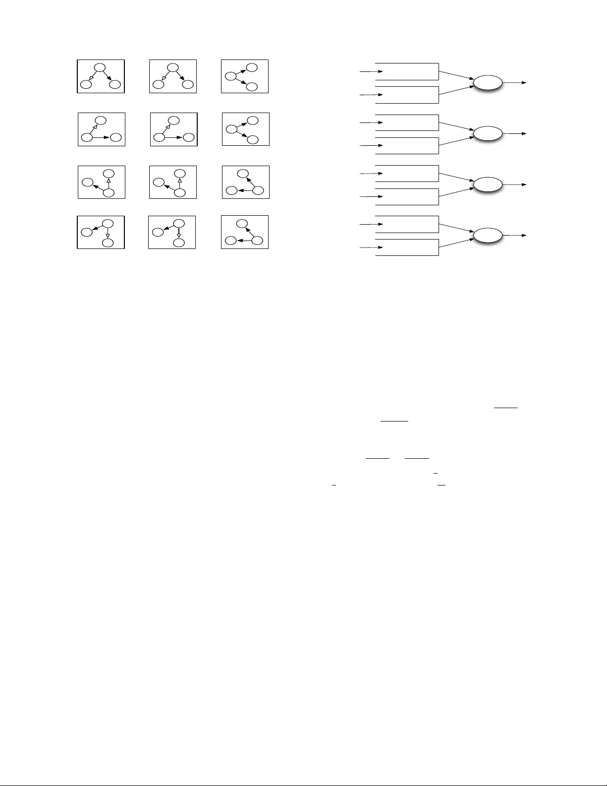
1 Network Capacity Region and Minimum Energy Function for a Delay-T olerant Mobile Ad Hoc Network Rahul Urg aonkar and Michael J. Neely Abstract —W e in vestigate two quantities of interest in a delay- tolerant mobile ad hoc network: the network capacity r egion and the minimum energy function. The network capacity region is defined as the set of all input rates that the network can stably support considering all possible scheduling and routing algorithms. Given any input rate v ector in this region, the minimum energy function establishes the minimum time av erage power r equired to support it. In this work, we consider a cell- partitioned model of a delay-tolerant mobile ad hoc network with general Markovian mobility . This simple model incorporates the essential features of locality of wireless transmissions as well as node mobility and enables us to exactly compute the corresponding network capacity and minimum energy function. Further , we propose simple schemes that offer performance guarantees that are arbitrarily close to these bounds at the cost of an increased delay . Index T erms —delay tolerant networks, mobile ad hoc network, capacity region, minimum energy scheduling, queueing analysis I . I N T R O D U C T I O N T wo quantities that characterize the performance limits of a mobile ad hoc network are the network capacity region and the minimum energy function. The network capacity region is defined as the set of all input rates that the network can stably support considering all possible scheduling and routing algorithms that conform to the given network structure. The minimum energy function is defined as the minimum time av erage power (summed ov er all users) required to stably support a gi ven input rate vector in this region. Here, by stability we mean that the input rates are such that for all users, the queues do not gro w to infinity and av erage delays are bounded. In this paper , we e xactly compute these quantities for a specific model of a delay-tolerant mobile ad hoc network. Asymptotic bounds on the capacity of static wireless net- works and mobile networks are dev eloped by [2], [3]. The work in [3] sho ws that for networks with full uniform mobility , if delay constraints are relaxed, a simple 2 -hop relay algorithm can support throughput that does not vanish as the number of network nodes N grows large. Recent work in [4] generalizes this model and inv estigates capacity scaling with non-uniform This w ork was supported in part by the DARP A IT -MANET Program under Grant W911NF-07-0028 and the National Science Foundation (NSF) under Grant OCE 0520324 and Career Grant CCF-0747525. This work was presented in part at the 4th International Symposium on Modeling and Optimization in Mobile, Ad Hoc, and W ireless Networks (WiOpt), Boston, MA, April 3-7, 2006. The authors are with the Department of Electrical Engineering, Uni- versity of Southern California, Los Angeles, CA 90089 USA (e-mail: ur- gaonka@usc.edu; mjneely@usc.edu). node mobility and heterogeneous nodes. Capacity-delay trade- offs in mobile ad hoc networks are considered in [8]–[12]. Flow-based characterization of the network capacity region is presented in se veral works (e.g., [7], [13], [14]). Howe ver , little work has been done in computing the exact capacity and energy expressions for these networks. Exceptions include a closed form expression for the capacity of a fixed grid network in [5], an expression for the exact information theoretic capacity for a single source multicast setting in a wireless erasure network [6], and an expression for the capacity of a mobile ad hoc network in [8] that uses a cell- partitioned structure. The work in [8] quantizes the network geography into a finite number of cells over which users mo ve, and assumes that a single packet can be transmitted between users who are currently in the same cell, while no transmission is possible between users currently in different cells. 1 In this work, we extend this model to more general scenar - ios allowing adjacent cell communication and different rate- power combinations. Specifically , we extend the simplified cell-partitioned model of [8] (which only allows same cell communication and considers i.i.d. mobility) to treat adjacent cell communication. W e establish exact capacity expressions for general Marko vian user mobility processes (possibly non- uniform), assuming only a well-defined steady-state location distribution for the users. Our analysis shows that, similar to [8], the capacity is only a function of the steady-state location distribution of the nodes and a 2 -hop relay algorithm is throughput optimal for this extended model as well. Further , our analysis illuminates the optimal decision strategies and precisely defines the throughput optimal control law for choos- ing between same cell and adjacent cell communication. W e then use this insight to design a simple 2 -hop relay algorithm that can stabilize the network for all input rates within the network capacity region. W e also compute an upper bound on the av erage delay under this algorithm. (Sec. III) W e next compute the exact expression for the minimum energy required to stabilize this network, for all input rates within capacity . Our result demonstrates a piece wise linear structure for the minimum energy function that corresponds to opportunistically using up successive transmission modes. Then we present a greedy algorithm whose av erage energy can be pushed arbitrarily close to the minimum energy at the cost of an increased delay . (Sec. IV) 1 Here a cell represents only a sub-region of the network. There are no base stations in the cells (i.e., this should not be confused with “cellular networks” that use base stations.) 2 R 1 R 2 R 2 R 2 R 1 R 2 R 1 Fig. 1. An illustration of the cell-partitioned network with same and adjacent cell communication. Cells that share an edge are assumed to be adjacent. Before proceeding further , we emphasize that the network capacity and minimum energy function derived in this paper are subject to the scheduling and routing constraints of our model as described in the next section. Specifically , in this work, we do not consider techniques that “mix” packets, such as network coding or cooperativ e communication, which can increase the network capacity and reduce energy costs. In fact, in Sec. V, we present an example scenario that shows how network coding in conjunction with the wireless broadcast advantage can increase the capacity for this model. Calculating the network capacity region and the minimum energy function when these strategies are allowed is an open problem in general in network information theory and is beyond the scope of this paper . I I . N E T W O R K M O D E L A. Cell-P artitioned Structur e W e use a cell-partitioned network model (Fig. 1) having C non-ov erlapping cells (not necessarily of the same size/shape). There are N users roaming from cell to cell over the network according to a mobility process. Each cell c ∈ { 1 , 2 , . . . , C } has a set of adjacent cells B c that a user can mo ve into from cell c . The maximum number of adjacent cells of any cell is bounded by a finite constant J . W e define the network user density as θ = N /C users/cell. For simplicity , N is assumed to be even and N ≥ 2 . Note that there could be “gaps” in the cell structure due to infeasible geographic locations. W e assume that the gaps do not partition the network, so that it is possible for a single user to visit all cells. W e assume C is the number of v alid cells, not including such gaps. B. Mobility Model T ime is slotted so that each user remains in its current cell for a timeslot and potentially moves to an adjacent cell at the end of the slot. W e assume that each user i moves independently of the other users according to a mobility process that is described by a finite state ergodic Markov Chain. In particular, let P = { P ij } C × C be the transition probability matrix of this Markov Chain. Then P ij represents the conditional probability that a user moves to cell j in the current slot giv en that it was in cell i in the last slot. Note that P ij > 0 only if j is an adjacent cell of i , i.e., j ∈ B i . It can be sho wn that the resulting mobility process has a well- defined steady-state location distribution π = { π c } 1 × C ov er the cells c ∈ { 1 , 2 , . . . , C } that satisfies π P = π and is the same for all users. Howe ver , this distribution could be non- uniform over the cells. W e assume that in each slot, users are aware of the set of other users in the same cell and in adjacent cells. Howe ver , the transition probabilities associated with the Markov Chain P are not necessarily kno wn. It can be shown (see, for example, [18]) that the mobility process discussed abov e has the following property . Let χ ( t ) ∈ { 1 , . . . , C } denote the location of a user in timeslot t . Then, for all integers d > 0 , there exist positive constants α, γ such that ∀ c ∈ { 1 , 2 , . . . , C } , the follo wing holds: π c (1 − αγ d ) ≤ P r [ χ ( t + d ) = c | χ ( t )] ≤ π c (1 + αγ d ) (1) where α > 1 and 0 < γ < 1 . Moreover , the decay factor γ is giv en by the second largest eigenv alue of the transition probability matrix P (see [17]). From this, it can be seen that for any  > 0 , choosing d = d log( /α ) log( γ ) e ensures that the conditional probability that the user is in cell c at time t + d is within π c  of the steady-state probability π c of being in cell c , irrespectiv e of the current location. This implies that the Markov Chain con verges to its steady-state probability distribution exponentially fast. Using the independence of user mobility processes, the following can be sho wn about functionals of the joint user location process ~ χ ( t ) : Lemma 1: Let ~ χ ( t ) = ( χ 1 ( t ) , . . . , χ N ( t )) be the vector of current user locations, where χ i ( t ) represents the cell of user i in slot t . Let f ( ~ χ ( t )) be any non-negati ve function of ~ χ ( t ) , i.e., f ( ~ χ ( t )) ≥ 0 ∀ ~ χ ( t ) . Define f av as the expectation of f ( ~ χ ( t )) over the steady-state distribution of ~ χ ( t ) : f av M = X c 1 ,c 2 ,...,c N f ( c 1 , . . . , c N ) N Y i =1 π c i Then for all d such that αγ d ≤ 1 N 2 , we ha ve f av (1 − 2 N αγ d ) ≤ E { f ( ~ χ ( t + d )) | ~ χ ( t ) } ≤ f av (1 + 2 N αγ d ) Pr oof: See Appendix A. C. T raf fic Model W e assume that there are N unicast sessions in the network with each node being the source of one session and the destination of another session. Pack ets are assumed to arri ve at the source of each session i according to an i.i.d. arriv al process A i ( t ) of rate λ i . W e assume that in any slot, the maximum number of arri v als to any session i is bounded, i.e., A i ( t ) ≤ A max . While our analysis holds for the general source-destination pairing, for simplicity , we assume that N is even with the following one-to-one pairing between users: 1 ↔ 2 , 3 ↔ 4 , . . . , ( N − 1) ↔ N , i.e., packets generated by user 1 are destined for user 2 and those generated by user 2 are destined for user 1 and so on. This assumption simplifies the computation of the capacity in closed form in Theorem 1 and will be used for the rest of the paper . 3 D. Communication Model W e assume that two users can communicate only if they are in the same cell or in adjacent cells. Further , if the communication takes place in the same cell, R 1 packets can be transmitted from the sender to the receiver if the sender uses full power . If the receiv er is in an adjacent cell, R 2 packets can be transmitted with full po wer . W e assume that R 1 and R 2 are non-negati ve integers and that R 1 ≥ R 2 . Power allocation is restricted to the set { 0 , 1 } , i.e., each user either uses zero power or full power . For simplicity , we assume that the communication cost consists only of the transmission power . The analysis presented can be easily extended to the case with non-zero reception po wer by defining the communication cost as the total power (including transmission and reception) required for sending R 1 ( R 2 ) packets from a transmitter to a receiv er in the same (adjacent) cell. W e allow at most one transmitter in a cell at any giv en time slot, though the cell may hav e multiple receiv ers (due to possible adjacent cell communication). Further, a user may potentially transmit and receive simultaneously . This model is conceiv able if the users in neighboring cells use orthogo- nal communication channels. This model allows us to treat scheduling decisions in each cell independently of all other cells, thereby enabling us to derive closed form expressions for capacity and minimum energy . E. Discussion of Model While an idealization, the cell-partitioned model captures the essential features of locality of wireless transmissions as well as node mobility and allows us to compute exact expressions for the network capacity and minimum energy function. This model is reasonable when nodes use non- interfering orthogonal channels in adjacent cells. W e also refer to Section I-A of [8] for further discussion on the cell- partitioned network assumption. In this work, we restrict our attention to network control algorithms that operate according to the network structure described abov e. A general algorithm within this class will make scheduling decisions about what packet to transmit, when, and to whom. For example, it may decide to transmit to a user in an adjacent cell rather than to some user in the same cell, e ven though the transmission rate is smaller . Howe ver , we assume that the packets themselves are kept intact and are not “mixed” (for example, using cooperativ e communication and/or network coding). Allowing such strategies can increase the capacity , although computing the exact capacity region remains a challenging open problem in general. In Sec. V, we present an example that shows how network coding in conjunction with the wireless broadcast adv antage can increase the capacity for this model. Howe ver , we note that if we remov e the broadcast feature, then the scenario considered in this paper becomes a network coding problem for multiple unicasts over an undirected graph, for which it is not yet known if network coding pro vides any gains ov er plain routing (see further discussion in [16]). I I I . N E T W O R K C A PAC I T Y In this section, we compute the exact capacity of the net- work model described in the previous section. For simplicity , we assume that all users receiv e packets at the same rate (i.e., λ i = λ for all i ). The capacity of the network is then described by a scalar quantity which denotes the maximum rate λ that the network can stably support. Recall that network user density θ = N /C users/cell. Then we ha ve the following: Theor em 1: The capacity of the network (in packets/slot) is giv en by: µ = ( R 1 q + R 1 p + R 2 q 0 + R 2 p 0 2 θ if R 1 ≥ 2 R 2 2 R 1 q +2 R 2 q 00 + R 1 p 00 + R 2 ( p 0 − q 0 ) 2 θ if 2 R 2 > R 1 ≥ R 2 where q = 1 C P C c =1 P r [ finding a source-destination pair in cell c in a timeslot] p = 1 C P C c =1 P r [ finding at least 2 users in cell c in a timeslot] q 0 = 1 C P C c =1 P r [ finding exactly 1 user in cell c and its destination in an adjacent cell in a timeslot] p 0 = 1 C P C c =1 P r [ finding exactly 1 user in cell c and at least 1 user in an adjacent cell in a timeslot] q 00 = 1 C P C c =1 P r [ finding no source-destination pair in cell c but at least 1 source-destination pair with an adjacent cell in a timeslot] p 00 = 1 C P C c =1 P r [ finding no source-destination pair in cell c and any adjacent cell but at least 2 users in the cell c in a timeslot] The probabilities in the summations above are the proba- bilities associated with the steady-state cell location distribu- tions of the users. Using the independence of user mobility processes and the same steady-state cell location distribution π = { π c } 1 × C for all users, we can exactly compute these probabilities for our model. These are gi ven by (see Appendix B for detailed deri vation): q = 1 C C X c =1  1 − (1 − π 2 c ) N 2  p = 1 C C X c =1  1 − (1 − π c ) N − N π c (1 − π c ) N − 1  q 0 = 1 C C X c =1  Π ad j ( c ) N π c (1 − π c ) N − 1  p 0 = 1 C C X c =1  1 − (1 − Π ad j ( c )) N − 1  N π c (1 − π c ) N − 1 q 00 = 1 C C X c =1 N 2 X i =1 2 i  N 2 i  π i c (1 − π c ) N − i  1 − (1 − Π ad j ( c )) i  p 00 = 1 C C X c =1 N 2 X i =2 2 i  N 2 i  π i c (1 − π c ) N − i (1 − Π ad j ( c )) i (2) Here, Π ad j ( c ) denotes the sum of the conditional steady-state probability of a user being in any adjacent cell of cell c given that this user is not in cell c , i.e., Π ad j ( c ) = 1 1 − π c P i ∈B c π i . Thus, the network can stably support users simultaneously communicating at any rate λ < µ . W e prove the theorem 4 in two parts. First, we establish the necessary condition by deriving an upper bound on the capacity of any stabilizing algorithm. Then, we establish sufficienc y by presenting a specific scheduling strategy and showing that the a verage delay is bounded under that strategy . A. Pr oof of Necessity Pr oof: Let Ψ be the set of all stabilizing scheduling policies. Consider an y particular policy ψ ∈ Ψ . Suppose it suc- cessfully delivers X ψ ab ( T ) packets from sources to destinations in volving “ a ” same cell transmissions and “ b ” adjacent cell transmissions in the interval (0 , T ) . Fix  > 0 . For stability , there must exist arbitrarily large values of T such that the total output rate is within  of total input rate. Thus: P ∞ a =0 P ∞ b =0 X ψ ab ( T ) T ≥ N λ −  (3) Define Y ψ ( T ) as the total number of packet transmis- sions in (0 , T ) under policy ψ . Then, Y ψ ( T ) is at least P ∞ a =0 P ∞ b =0 ( a + b ) X ψ ab ( T ) (because these many packets were certainly deli vered). Thus, we hav e 1 T Y ψ ( T ) ≥ 1 T ∞ X a =0 ∞ X b =0 ( a + b ) X ψ ab ( T ) ≥ 1 T X a + b< 2 X ψ ab ( T ) + 2 T X a + b ≥ 2 X ψ ab ( T ) ≥ 1 T X a + b< 2 X ψ ab ( T ) + 2( N λ −  ) − 2 T X a + b< 2 X ψ ab ( T ) where the last inequality is obtained using (3). Hence, noting that  can be chosen to be arbitrarily small, we hav e: λ ≤ lim T →∞ Y ψ ( T ) + X ψ 10 ( T ) + X ψ 01 ( T ) 2 T N (4) Define Y ψ c ( τ ) as the total number of packet transmissions in cell c at timeslot τ under policy ψ . Also define X ψ 10 ,c ( τ ) and X ψ 01 ,c ( τ ) as the number of packets deliv ered by same cell direct and adjacent cell direct transmission respectively in cell c at timeslot τ . Then Y ψ ( T ) + X ψ 10 ( T ) + X ψ 01 ( T ) can be written as a sum ov er all timeslots τ ∈ (0 , T ) and all cells c as follo ws: Y ψ ( T ) + X ψ 10 ( T ) + X ψ 01 ( T ) = T − 1 X τ =0 C X c =1  Y ψ c ( τ ) + X ψ 10 ,c ( τ ) + X ψ 01 ,c ( τ )  ≤ T − 1 X τ =0 C X c =1 max ω ∈ Ψ  ˆ Y ω c ( τ ) + ˆ X ω 10 ,c ( τ ) + ˆ X ω 01 ,c ( τ )  (5) where ˆ Y ω c ( τ ) denotes the total number of packet transmission opportunities in cell c at timeslot τ under any policy ω . Similarly , ˆ X ω 10 ,c ( τ ) and ˆ X ω 01 ,c ( τ ) denote the total number of packet transmission opportunities that use same cell direct and adjacent cell direct transmissions respectiv ely in cell c at timeslot τ . Note that these do not depend on the queue backlogs and therefore can be dif ferent from the actual number of packet transmissions (for e xample, when enough packets are not av ailable). Let ˆ Z ω c ( τ ) = ˆ Y ω c ( τ ) + ˆ X ω 10 ,c ( τ ) + ˆ X ω 01 ,c ( τ ) . Also define the following indicator decision variables for any policy ω for some τ ∈ (0 , T ) and c ∈ { 1 , 2 , . . . , C } : I 1 c ( τ ) =    1 if a same cell direct transmission can be scheduled in cell c in slot τ 0 else I 2 c ( τ ) =    1 if a same cell relay transmission can be scheduled in cell c in slot τ 0 else I 3 c ( τ ) =    1 if an adjacent cell direct transmission can be scheduled in cell c in slot τ 0 else I 4 c ( τ ) =    1 if an adjacent cell relay transmission can be scheduled in cell c in slot τ 0 else Note that the transmission rates associated with these decision variables are R 1 , R 1 , R 2 and R 2 respectiv ely . Then, we can express ˆ Z ω c ( τ ) as follows: ˆ Z ω c ( τ ) = ˆ Y ω c ( τ ) + ˆ X ω 10 ,c ( τ ) + ˆ X ω 01 ,c ( τ ) = R 1 I 1 c ( τ ) + R 1 I 2 c ( τ ) + R 2 I 3 c ( τ ) + R 2 I 4 c ( τ ) + ˆ X ω 10 ,c ( τ ) + ˆ X ω 01 ,c ( τ ) = R 1 I 1 c ( τ ) + R 1 I 2 c ( τ ) + R 2 I 3 c ( τ ) + R 2 I 4 c ( τ ) + R 1 I 1 c ( τ ) + R 2 I 3 c ( τ ) = 2 R 1 I 1 c ( τ ) + R 1 I 2 c ( τ ) + 2 R 2 I 3 c ( τ ) + R 2 I 4 c ( τ ) Note that under an y scheduling policy , only one of the decision variables can be 1 and the rest are 0 . Thus, the preference order for decisions to maximize ˆ Z ω c ( τ ) is e vident. Specifically , it would be I 1 c ( τ )  I 2 c ( τ )  I 3 c ( τ )  I 4 c ( τ ) when R 1 ≥ 2 R 2 and I 1 c ( τ )  I 3 c ( τ )  I 2 c ( τ )  I 4 c ( τ ) when R 2 ≤ R 1 < 2 R 2 . Thus, in each cell c , ˆ Z ω c ( τ ) is maximized by the policy ω that chooses the scheduling decisions in this preference order, choosing a less preferred decision only when none of the more preferred decisions are possible in that cell. Define Z c ( τ ) = max ω ∈ Ψ ˆ Z ω c ( τ ) . Then using (4) and (5), we hav e λ ≤ lim T →∞ 1 2 T N T − 1 X τ =0 C X c =1 Z c ( τ ) As Z c ( τ ) can take only a finite number of values (namely R 1 , R 2 , 2 R 1 , 2 R 2 and 0 ) and is a function of the current state of the ergodic user location processes, the time average of Z c ( τ ) is exactly equal to its expectation with respect to the steady-state user location distribution. Thus, the bound abov e can be computed by calculating the expectation of Z c ( τ ) using the steady-state probabilities associated with the indicator variables and summing ov er all cells. When R 1 ≥ 2 R 2 , this 5 is gi ven by: lim T →∞ 1 2 T N T − 1 X τ =0 C X c =1 Z c ( τ ) = 1 2 N C X c =1 E { Z c ( τ ) } = 2 R 1 q + R 1 ( p − q ) + 2 R 2 q 0 + R 2 ( p 0 − q 0 ) 2 θ and when R 2 ≤ R 1 < 2 R 2 , this is gi ven by: lim T →∞ 1 2 T N T − 1 X τ =0 C X c =1 Z c ( τ ) = 1 2 N C X c =1 E { Z c ( τ ) } = 2 R 1 q + 2 R 2 q 00 + R 1 p 00 + R 2 ( p 0 − q 0 ) 2 θ This establishes the necessary condition for the network capacity . Note that the abov e preference order clearly spells out the structure of the throughput optimal strategy . Specifically , depending on the values of R 1 and R 2 , this order can be used to decide between same cell relay and adjacent cell direct transmission. W e use this insight to design a throughput- optimal 2 -hop relay algorithm in the next section. Also note the factor of 2 with the decision variables corresponding to direct source-destination transmission. Intuitiv ely , each such transmission opportunity is better than a similar opportunity between source-relay or relay-destination by a f actor of 2 since the indirect transmissions need twice as many opportunities to deli ver a giv en number of packets to the destination as compared to direct transmissions. B. Pr oof of Sufficiency Now we present an algorithm that makes stationary , ran- domized scheduling decisions independent of the queue back- logs and show that it gives bounded delay for any rate λ < µ , i.e., there exists a ρ such that 0 ≤ ρ < 1 and λ = ρµ . W e only consider the case when R 1 ≥ 2 R 2 . The other case is similar and is not discussed. 2-Hop Relay Algorithm: Every timeslot, for all cells, do the follo wing: 1) If there exists a source-destination pair in the cell, ran- domly choose such a pair (uniformly over all such pairs in the cell). If the source has ne w packets for the destination, transmit at rate R 1 . Else remain idle. 2) If there is no source-destination pair in the cell b ut there are at least 2 users in the cell, randomly designate one user as the sender and another as the receiv er . Then, with probability 1 − δ 2 (where 0 < δ < 1 and δ = δ ( ρ ) to be determined later), perform the first action below . Else, perform the second. a) Send new Relay pack ets in same cell : If the transmitter has ne w packets for its destination, transmit at rate R 1 . Else remain idle. b) Send Relay packets to their Destination in same cell : If the transmitter has packets for the receiv er, transmit at rate R 1 . Else remain idle. 3) If there is only 1 user in the cell and its destination is present in one of the adjacent cells, transmit at rate R 2 if ne w packets present. Else remain idle. 4) If there is only 1 user in the cell and its destination is not present in one of the adjacent cells but there is at least one user in an adjacent cell, randomly designate one such user as the receiver and the only user in the cell as the transmitter . Then, with probability 1 − δ 2 (where 0 < δ < 1 and δ = δ ( ρ ) to be determined later), perform the first action belo w . Else, perform the second. a) Send new Relay packets in adjacent cell : If the trans- mitter has new packets for its destination, transmit at rate R 2 . Else remain idle. b) Send Relay packets to their Destination in adjacent cell : If the transmitter has packets for the recei ver , transmit at rate R 2 . Else remain idle. This algorithm is motiv ated by the proof of necessity of Theorem 1 since it follo ws the same preference order in making scheduling decisions. Note that this algorithm restricts the path lengths of all packets to at most 2 hops because any packet that has been transmitted to a relay node is restricted from being transmitted to an y other node except its destination. T o analyze the performance of this algorithm, we make use of a L yapunov drift analysis [7]. Consider a network of N queues operating in slotted time, and let ~ U ( t ) = ( U 1 ( t ) , U 2 ( t ) , . . . , U N ( t )) represent the vector of backlogged packets in each of the queues at timeslot t . Let L ( ~ U ( t )) be a non-negati ve function of the unfinished work ~ U ( t ) , called a L yapunov function. Define the conditional L yapunov drift ∆( t, d ) at time t > d (where d ≥ 0 in a fixed integer) as follows: ∆( t, d ) M = E n L ( ~ U ( t + 1)) − L ( ~ U ( t )) | ~ U ( t − d ) o Then we ha ve the following lemma. Lemma 2: L yapunov Drift Lemma : If there exists a positi ve integer d such that for all timeslots t > d and for all ~ U ( t ) , the conditional L yapunov drift ∆( t, d ) satisfies: ∆( t, d ) ≤ B −  N X i =1 U i ( t − d ) (6) for some positi ve constants B and  , and if E n L ( ~ U ( d )) o < ∞ , then the network is stable, and we hav e the following bound on the time average total queue backlog: lim sup t →∞ 1 t t − 1 X τ =0 N X i =1 E { U i ( τ ) } ≤ B  (7) Pr oof: This can be shown using a telescoping sum technique (similar to related proof in [7]) and is omitted for brevity . W e now make use of this lemma to analyze the performance of the 2 -Hop Relay Algorithm. Theor em 2: For the cell partitioned network (with N nodes 6 and C cells) as described in Sec. II, with capacity µ = R 1 p + R 2 p 0 + R 1 q + R 2 q 0 2 θ and input rate λ for each user such that λ = ρµ for some 0 ≤ ρ < 1 , and user mobility model as described in Sec. II-B, the average packet delay D under the 2 -Hop Relay Algorithm with δ = 1 − ρ 4 satisfies: D ≤ B N (2 d + 1) λµκ (1 − ρ ) (8) where B is a constant given by (11), κ is a positi ve constant giv en by κ = R 1 p + R 2 p 0 − R 1 q − R 2 q 0 R 1 p + R 2 p 0 + R 1 q + R 2 q 0 , and d is a finite integer that is related to the mixing time of the joint user mobility process and is gi ven by d = l log( 8 N 2 α 1 − ρ ) log(1 /γ ) m . Pr oof: Let U ( c ) i ( t ) represent the total backlog of type c (i.e., number of packets destined for node c ) that are queued up in node i at time t . The queueing dynamics of U ( c ) i ( t ) satisfies the follo wing for all c 6 = i : U ( c ) i ( t + 1) ≤ max h U ( c ) i ( t ) − X b µ ( c ) ib ( t ) , 0 i + X a µ ( c ) ai ( t ) + A ( c ) i ( t ) (9) where A ( c ) i ( t ) = number of new type c arriv als to source node i at the beginning of timeslot t and µ ( c ) ab ( t ) = rate offered to type c packets in timeslot t with node a as transmitter and node b as receiv er . The abov e is an inequality because the actual number of packets transmitted from the other nodes to node i (for relaying) could be less than the incoming transmission rate P a µ ( c ) ai ( t ) when these nodes do not have enough packets. Now define a L yapunov function L ( ~ U ( t )) = P N i =1 P c 6 = i ( U ( c ) i ( t )) 2 . Using (9), the conditional L yapunov drift ∆( t, d ) can be expressed as follows: ∆( t, d ) ≤ B N − 2 N X i =1 X c 6 = i E ( U ( c ) i ( t ) ×  X b µ ( c ) ib ( t ) − X a µ ( c ) ai ( t ) − A ( c ) i ( t )  | ~ U ( t − d ) ) (10) Here, B is giv en by: B = ( A max + µ in max ) 2 + ( µ out max ) 2 (11) where µ in max = maximum transmission rate into any node = R 1 + J R 2 , where J is the maximum number of adjacent cells of any cell (Sec. II-A) and µ out max = maximum transmission rate out of an y node = R 1 . W e now use the following sample path relations to express (10) in terms of the queue backlog values at time ( t − d ) . Specifically , we ha ve the following for all t > d where d is a positiv e integer (to be determined later) for all i 6 = c . X c 6 = i U ( c ) i ( t − d ) + d ( A max + µ in max ) ≥ X c 6 = i U ( c ) i ( t ) X c 6 = i U ( c ) i ( t − d ) − dµ out max ≤ X c 6 = i U ( c ) i ( t ) These follow by noting that the queue backlog at time t cannot be smaller than the queue backlog at time ( t − d ) minus the maximum possible departures in duration ( t − d, d ) . Similarly , it cannot be larger than the queue backlog at time ( t − d ) plus the maximum possible arriv als in duration ( t − d, d ) . Using these, we can express (10) in terms of the “delayed” queue backlogs U ( c ) i ( t − d ) as follows: ∆( t, d ) ≤ B N (2 d + 1) − 2 N X i =1 X c 6 = i U ( c ) i ( t − d ) × E ( X b µ ( c ) ib ( t ) − X a µ ( c ) ai ( t ) − A ( c ) i ( t ) | ~ U ( t − d ) ) (12) Let T ( t − d ) = ( ~ χ ( t − d ) , ~ U ( t − d )) represent the composite system state at time ( t − d ) giv en by the user locations and queue backlogs. Since the 2 -Hop Relay Algorithm makes con- trol decisions only as a function of the current user locations, the resulting service rates are functionals of the Marko vian mobility processes. By the Markovian property of the ~ χ ( t − d ) process, any functionals of this also conv erge exponentially fast to their steady-state v alues. Thus, using Lemma 1, when αγ d ≤ 1 / N 2 , we ha ve the following bounds: E ( X b µ ( c ) ib ( t ) | ~ U ( t − d ) ) ≥  X b µ ( c ) ib  (1 − 2 N αγ d ) (13) E ( X a µ ( c ) ai ( t ) | ~ U ( t − d ) ) ≤  X a µ ( c ) ai  (1 + 2 N αγ d ) (14) where µ ( c ) ib , µ ( c ) ai are the steady-state service rates achie ved by the 2 -Hop Relay Algorithm. W e now compute these v alues and use the inequalities (13), (14) to obtain a bound on (12). W e hav e the following 2 cases: 1) Node i Generates T ype c P ack ets: In this case, E n A ( c ) i ( t ) o = λ and P a µ ( c ) ai ( t ) = 0 (since under the 2 - Hop Relay Algorithm, a source node would nev er get back a packet that it generates). T o calculate P b µ ( c ) ib , we note that the outgoing service rate for packets generated by the source is equal to the sum of the rate at which the source is scheduled to transmit directly to its destination and the rate at which it is scheduled to transmit type c packets to any of the relay nodes. Let these rates be r 1 and r 2 respectiv ely . Also let the trans- mission rate at which it is scheduled to transmit relay packets to their destinations be r 3 . Since the 2 -Hop Relay Algorithm only schedules transmissions of these types, the total rate of transmissions over the network is giv en by N ( r 1 + r 2 + r 3 ) . Using the probability of choosing source-relay and relay- destination transmissions, we hav e: r 2 = 1 − δ 1+ δ r 3 . In the 2 -Hop Relay Algorithm, a direct source-to-destination transmission is scheduled whenever there is a source-destination pair in the same cell or there is only 1 node in a cell and its destination is in an adjacent cell (and independent of the actual queue backlog values). Thus, using the definitions of q and q 0 from the statement of Theorem 1, we hav e: N r 1 = C ( R 1 q + R 2 q 0 ) . Similarly , the sum total transmissions in the network can be expressed in terms of the quantities p and p 0 as follows: N ( r 1 + r 2 + r 3 ) = C ( R 1 p + R 2 p 0 ) . Using these to solve for r 1 , r 2 , r 3 and simplifying, we ha ve r 1 = µ (1 − κ ) , r 2 = µκ (1 − δ ) , r 3 = µκ (1 + δ ) (15) 7 where κ M = R 1 p + R 2 p 0 − R 1 q − R 2 q 0 R 1 p + R 2 p 0 + R 1 q + R 2 q 0 . Note that 0 < κ < 1 (since p > q and p 0 > q 0 ). Therefore, we ha ve: X b µ ( c ) ib = r 1 + r 2 = µ − µκδ Let δ = 1 − ρ 4 and α γ d = δ 2 N 2 = 1 − ρ 8 N 2 . Note that this choice of δ represents a valid probability since 0 ≤ ρ < 1 . Then, using (13), the last term of (12) under this case can be expressed as: E ( X b µ ( c ) ib ( t ) − X a µ ( c ) ai ( t ) − A ( c ) i ( t ) | ~ U ( t − d ) ) ≥  X b µ ( c ) ib  (1 − 2 N αγ d ) − λ = ( µ − µκδ )(1 − δ N ) − ρµ ≥ µ h (1 − δ ) 2 − ρ i ≥ µ (1 − 2 δ − ρ ) = µ (1 − ρ ) 2 where we used the fact that (1 − κδ )(1 − δ N ) ≥ (1 − δ ) 2 . 2) Node i Relays T ype c P ackets: Note that N > 2 for this case to happen. From our traffic model, we know that in this case A ( c ) i ( t ) = 0 for all t . Further , under the 2 -Hop Relay Algorithm, µ ( c ) ai ( t ) > 0 only if node a is the source for type c packets. Also µ ( c ) ib ( t ) > 0 only if b = c . T o compute P b µ ( c ) ib and P a µ ( c ) ai for this case, note that the 2 -Hop Relay Algorithm schedules relay transmissions such that all ( N − 2) relay packet types are equally likely . Thus we hav e: X b µ ( c ) ib = r 3 N − 2 , X a µ ( c ) ai = r 2 N − 2 Let δ = 1 − ρ 4 and αγ d = δ 2 N 2 = 1 − ρ 8 N 2 . Then, using (13), (14), the last term of (12) under this case can be expressed as: E ( X b µ ( c ) ib ( t ) − X a µ ( c ) ai ( t ) − A ( c ) i ( t ) | ~ U ( t − d ) ) ≥  X b µ ( c ) ib  (1 − 2 N αγ d ) −  X a µ ( c ) ai  (1 + 2 N αγ d ) =  X b µ ( c ) ib − X a µ ( c ) ai  −  X b µ ( c ) ib + X a µ ( c ) ai  δ N = ( r 3 − r 2 ) − ( r 3 + r 2 ) δ N N − 2 = 2 µκδ N − 2  1 − 1 N  ≥ µκ (1 − ρ ) 2 N where we used (15). Combining these tw o cases, with δ = 1 − ρ 4 and αγ d = 1 − ρ 8 N 2 : E ( X b µ ( c ) ib ( t ) − X a µ ( c ) ai ( t ) − A ( c ) i ( t ) | ~ U ( t − d ) ) ≥ µκ (1 − ρ ) 2 N Using this in (12), we get: ∆( t, d ) ≤ B N (2 d + 1) − µκ (1 − ρ ) N N X i =1 X c 6 = i U ( c ) i ( t − d ) This is in a form that fits (6). Using the L yapunov Drift Lemma, we get lim sup t →∞ 1 t t − 1 X τ =0 X i 6 = c E n U ( c ) i ( τ ) o ≤ B N 2 (2 d + 1) µκ (1 − ρ ) (16) 0.05 0.1 0.15 0.2 0.25 0.3 0.35 0.4 0.45 0.5 0 5000 10000 15000 input rate ! (packets/slot) average packet delay (slots) x = 0.05 x = 0.1 x = 0.25 x = 0.5 analytical bound for i.i.d. mobility Fig. 2. A verage packet delay under the 2 -Hop Relay Algorithm in a network of 16 cells with 20 nodes for different mixing times of the mobility process. The total input rate into the network is N λ . Thus, using Little’ s Theorem, the av erage delay per packet is bounded by B N (2 d +1) λµκ (1 − ρ ) . C. Discussion and Simulation Example The proof of the capacity for the cell-partitioned network can be used to consider more general scheduling restrictions. From (5), it amounts to: λ ≤ 1 2 N E ( max ω ∈ Ψ C X c =1  Y ω c ( t ) + X ω 10 ,c ( t ) + X ω 01 ,c ( t )  ) If the bound on the right hand side can be achiev ed by any policy (potentially randomized) that takes decisions only as a function of the current network state, then we can design a deterministic policy that is throughput optimal by scheduling to maximize P C c =1  Y ω c ( t ) + X ω 10 ,c ( t ) + X ω 01 ,c ( t )  subject to the network restrictions. For the specific cell-partitioned model considered here, this maximization is achie ved by following the preference order of the decision variables in each cell separately as described earlier . This enables us to exactly compute the capacity of the network. It is possible to do the same for e xtensions to this model inv olving other constraints. For e xample, under the constraint that a user cannot simultane- ously transmit and recei ve, the above maximization becomes a maximum-weight match problem. Similarly , one could allow more than one transmitter per cell, in which case we would need to define more indicator decision variables for all possible control options. W e next consider an example network consisting of 20 nodes and 16 cells as sho wn in Fig. 1. The nodes mo ve from one cell to another independently according to a Markovian random walk. Specifically , at the end of e very slot, a node stays in its current cell with probability (1 − x ) , else it decides to move randomly one step in either the North, W est, South, or East directions with probability x . If there is no feasible adjacent cell, then the user remains in the current cell. It can be sho wn that the resulting steady-state location distribution is uniform over all cells for all 0 ≤ x < 1 . Thus, π c = 1 16 for all cells c . Next we assume that R 1 = 2 and R 2 = 1 packets/slot. Then using Theorem 1, the capacity for this network is giv en by µ = R 1 q + R 1 p + R 2 q 0 + R 2 p 0 2 θ and can be calculated exactly . Specifically , we get p = 0 . 358 , q = 8 0 . 038 , p 0 = 0 . 357 , q 0 = 0 . 073 and the network capacity is giv en by µ = 0 . 489 packets/slot. W e next simulate the 2 -Hop Relay Algorithm on this network. New packets arriv e at each source node according to independent Bernoulli processes, so that a single packet arriv es i.i.d. with probability λ e very slot. In Fig. 2, we plot the average packet delay vs. λ for different values of x . W e also plot the analytical bound (8) of Theorem 2 for the i.i.d. mobility case (for which d = 0 ). It can be seen that the av erage delay goes to infinity as λ is pushed closer to the capacity µ = 0 . 489 packets/slot (shown by the vertical line in Fig. 2). While the network capacity is the same for all values of x (since x does not affect the steady-state location distribution), the av erage delay increases as x becomes smaller . This is because a smaller x implies a larger value for the parameter d leading to larger delay as suggested by the delay bound (8) in Theorem 2. Thus, the 2 -Hop Relay Algorithm is able to support all input rates within the network capacity with finite av erage delay . Howe ver , its delay performance is not necessarily the best. For example, when the input rate is small (say λ = 0 . 1 packets/slot), the av erage delay is more than 100 slots. Note that the 2 -Hop Relay Algorithm makes scheduling decisions purely based on the current user locations and restricts all packets to at most 2 hops. It does not attempt to optimize the delay in the network. The delay performance may be improv ed using alternative scheduling strategies that do not restrict packets to at most 2 hops. For example, backlog aware scheduling and routing (e.g., [7]) or schemes that e xploit the mobility pattern of the users (e.g., [15]) may offer better delay performance. I V . M I N I M U M E N E R G Y F U N C T I O N W e now in vestigate the minimum energy function of the cell-partitioned network under consideration. Recall that in our network model, each user either uses zero power or full power . Further , R 1 ( R 2 ) packets can be transmitted from the sender to the receiver in the same (adjacent) cell if the sender uses full po wer . The minimum energy function Φ( λ ) is defined as the minimum time av erage energy required to stabilize an input rate λ per user, considering all possible scheduling and routing algorithms that conform to the given network structure. W e exactly compute this function for our network model. Specif- ically , we assume that all users receive packets at the same rate (i.e., λ i = λ for all i ). Also, we consider the case when R 1 ≥ 2 R 2 ( Φ( λ ) for the case when R 1 < 2 R 2 has a different expression, but the proof is similar). Theor em 3: The minimum energy function Φ( λ ) per user for the cell-partitioned network as described in Sec. II with R 1 ≥ 2 R 2 is a piecewise linear curve giv en by the following: Φ( λ ) =              λ R 1 if C 1 q θ + 2 R 1  λ − 2 R 1 q 2 θ  if C 2 p θ + 1 R 2  λ − R 1 ( p + q ) 2 θ  if C 3 p + q 0 θ + 2 R 2  λ − R 1 ( p + q )+2 R 2 q 0 2 θ  if C 4 where C 1 ≡ 0 ≤ λ < R 1 q θ , C 2 ≡ R 1 q θ ≤ λ < R 1 ( p + q ) 2 θ , C 3 ≡ R 1 ( p + q ) 2 θ ≤ λ < R 1 ( p + q )+2 R 2 q 0 2 θ , C 4 ≡ R 1 ( p + q )+2 R 2 q 0 2 θ ≤ λ < µ . Thus, the network can stably support users simultaneously communicating at any rate λ < µ with an energy cost that can be pushed arbitrarily close to Φ( λ ) (at the cost of increased delay). W e prove the theorem in two parts. First, we establish the necessary condition by deri ving a lower bound on the energy cost of any stabilizing algorithm. Then, we establish sufficienc y by presenting a specific scheduling policy and showing that the av erage delay is bounded under that policy . A. Pr oof of Necessity Pr oof: Consider an y scheduling strategy that stabilizes the system. Let X ab ( T ) denote the number of packets delivered by the strategy from sources to destinations in time interval (0 , T ) that inv olves exactly a same cell and b adjacent cell transmissions. For simplicity , assume that the strategy is er- godic and yields well defined time av erage energy expenditure per user e and well defined time average values for x ab where: x ab M = lim T →∞ X ab ( T ) T (17) The av erage energy cost per user e of this policy satisfies: e ≥ X a,b  a R 1 + b R 2  x ab N (18) This follows by noting that enough packets may not be av ailable during a transmission. Note that x 00 = 0 , and so the only possible non-zero x ab variables are for ( a, b ) pairs that are integers, non-negati ve, and such that ( a, b ) 6 = (0 , 0) . Let x = ( x ab ) represent the collection of x ab variables, and note that these variables must satisfy the constraint x ∈ Ω 0 ∩ Ω 1 ∩ Ω 2 ∩ Ω 3 , where the four constraint sets are defined below: Ω 0 M = ( x      X ( a,b ) 6 =(0 , 0) x ab = N λ ) Ω 1 M = ( x      x 10 R 1 ≤ c 1 ) Ω 2 M = ( x      1 R 1 X a ax a 0 ≤ c 1 + c 2 ) Ω 3 M = ( x      1 R 1 X a ax a 0 + x 01 R 2 ≤ c 1 + c 2 + c 3 ) where c 1 is the maximum rate of source-destination trans- mission opportunities in the same cell, c 1 + c 2 is the maxi- mum rate of all possible same cell transmission opportunities and c 1 + c 2 + c 3 is the maximum rate of all same cell or source-destination adjacent cell transmission opportunities. Here, these quantities are summed over all cells. Using the definitions of p, q and q 0 from the statement of Theorem 1, we know that c 1 = C q , c 1 + c 2 = C p, c 1 + c 2 + c 3 = C ( p + q 0 ) . For example, ( c 1 + c 2 + c 3 ) can be written as 1 T P T t =0  X 1 ( t ) + X 2 ( t ) + X 3 ( t )  where X 1 ( t ) is the maximum number of direct same cell opportunities, X 2 ( t ) is the maximum number of indirect same cell opportunities given all direct opportunities are used and X 3 ( t ) is the maximum number of direct adjacent cell opportunities given all same cell opportunities are used. 9 Since only one of these three opportunities can used is a gi ven cell in a timeslot, the maximum total sum is fixed and hence c 1 + c 2 + c 3 = C ( p + q 0 ) . Define f ( x ) M = P a,b  a R 1 + b R 2  x ab N , which is simply the right hand side of (18). Because e ≥ f ( x ) , and because x ∈ Ω 0 ∩ Ω 1 ∩ Ω 2 ∩ Ω 3 , we ha ve: e ≥ inf x ∈ Ω 0 ∩ Ω 1 ∩ Ω 2 ∩ Ω 3 f ( x ) (19) Furthermore, for any function g ( x ) such that g ( x ) ≤ f ( x ) for all x , and for any set ˜ Ω that contains the set Ω 0 ∩ Ω 1 ∩ Ω 2 ∩ Ω 3 , we hav e: e ≥ inf x ∈ ˜ Ω g ( x ) (20) This follows because the function to be minimized is smaller, and the infimum is taken ov er a less restrictive set. W e now define four ne w constraint sets ˜ Ω 0 , ˜ Ω 1 , ˜ Ω 2 , ˜ Ω 3 as follo ws: ˜ Ω 0 M = Ω 0 ˜ Ω 1 M = Ω 1 ˜ Ω 2 M = ( x      x 10 R 1 + 2 R 1 X a ≥ 2 x a 0 ≤ c 1 + c 2 ) ˜ Ω 3 M = ( x      x 10 R 1 + 2 R 1 X a ≥ 2 x a 0 + x 01 R 2 ≤ c 1 + c 2 + c 3 ) It can be seen that each of Ω 0 , Ω 1 , Ω 2 , Ω 3 is a subset of ˜ Ω 0 , ˜ Ω 1 , ˜ Ω 2 , ˜ Ω 3 . Therefore, Ω 0 ∩ Ω 1 ∩ Ω 2 ∩ Ω 3 is a subset of ˜ Ω 0 ∩ ˜ Ω 1 ∩ ˜ Ω 2 ∩ ˜ Ω 3 . Note that since 2 R 1 ≤ 1 R 2 , we have the following: 1 R 1 < 2 R 1 ≤ 1 R 2 < 2 R 2 (21) W e now compute four different bounds for e , each having the form e ≥ αλ + β . These bounds define the four piecewise linear regions of Φ( λ ) . 1) First note that f ( x ) ≥ 1 R 1 P a,b x ab N . This follo ws from the definition of f ( x ) . Therefore taking g ( x ) = 1 R 1 P a,b x ab N , we ha ve: e ≥ inf x ∈ ˜ Ω 0 1 R 1 X a,b x ab N Because ˜ Ω 0 is giv en by P a,b x ab = N λ , the above infimum is equal to λ R 1 . Thus, we hav e our first linear constraint for any algorithm that yields a time average energy of e : e ≥ λ R 1 (22) 2) Next note that f ( x ) ≥ x 10 N R 1 + 2 R 1 P a,b ( a,b ) 6 =(1 , 0) x ab N . This is because a R 1 + b R 2 ≥ 2 R 1 for any non-negati ve integer pair ( a, b ) such that ( a, b ) 6 = { (0 , 0) , (1 , 0) } (using (21)). Therefore, taking this lower bound of f ( x ) as g ( x ) , we hav e: e ≥ inf x ∈ ˜ Ω 0 ∩ ˜ Ω 1 " x 10 N R 1 + 2 R 1 X a,b ( a,b ) 6 =(1 , 0) x ab N # The right hand side is equal to the solution of the following: Minimize: x 10 N R 1 + 2 R 1 X a,b ( a,b ) 6 =(1 , 0) x ab N Subject to: X a,b x ab = N λ x 10 R 1 ≤ c 1 The abov e optimization is equiv alent to minimizing x 10 N R 1 + 2 N R 1 ( N λ − x 10 ) subject to x 10 R 1 ≤ c 1 . The solution is clearly to choose x 10 = R 1 c 1 , and hence we have: e ≥ 2 λ R 1 − c 1 N = q θ + 2 R 1  λ − 2 R 1 q 2 θ  (23) 3) Next we have f ( x ) ≥ x 10 N R 1 + 2 R 1 X a ≥ 2 x a 0 N + 1 R 2 X a,b b 6 =0 x ab N which follows from the definition of f ( x ) and because 1 R 2 ≤ b R 2 for all positiv e b ≥ 1 . Thus, taking this lo wer bound of f ( x ) as g ( x ) , we ha ve: e ≥ inf x ∈ ˜ Ω 0 ∩ ˜ Ω 1 ∩ ˜ Ω 2 " x 10 N R 1 + 2 R 1 X a ≥ 2 x a 0 N + 1 R 2 X a,b b 6 =0 x ab N # This is equi valent to the following minimization: Minimize: x 10 N R 1 + 2 N R 1 X a ≥ 2 x a 0 + 1 N R 2  N λ − x 10 − X a ≥ 2 x a 0  Subject to: x 10 R 1 ≤ c 1 x 10 R 1 + 2 R 1 X a ≥ 2 x a 0 ≤ c 1 + c 2 where we have aggregated the constraint P a,b x ab = N λ into the objectiv e. The coefficients multiplying x 10 and P a ≥ 2 x a 0 are both ne gati ve, so that the above optimiza- tion is solved when x 10 + 2 P a ≥ 2 x a 0 = R 1 ( c 1 + c 2 ) . Similarly , it can be sho wn that above optimization is solved when x 10 = R 1 c 1 . This yields: e ≥ λ R 2 + ( c 1 + c 2 ) N − R 1 N R 2  c 1 + c 2 2  = p θ + 1 R 2  λ − R 1 ( p + q ) 2 θ  (24) 4) Finally , note that f ( x ) ≥ x 10 N R 1 + 2 R 1 X a ≥ 2 x a 0 N + x 01 N R 2 + 2 R 2 X b ≥ 2 x ab N which follows from the definition of f ( x ) as well as because 2 R 2 ≤ b R 2 for all b ≥ 2 . T aking this lo wer bound 10 of f ( x ) as g ( x ) , we ha ve: e ≥ inf x ∈ ˜ Ω " x 10 N R 1 + 2 R 1 X a ≥ 2 x a 0 N + x 01 N R 2 + 2 R 2 X b ≥ 2 x ab N # where ˜ Ω = ˜ Ω 0 ∩ ˜ Ω 1 ∩ ˜ Ω 2 ∩ ˜ Ω 3 . This is equiv alent to the following minimization (using P a,b x ab = N λ ): Minimize: x 10 N R 1 + 2 N R 1 X a ≥ 2 x a 0 + x 01 N R 2 + 2 N R 2  N λ − x 10 − X a ≥ 2 x a 0 − x 01  Subject to: x 10 R 1 ≤ c 1 x 10 R 1 + 2 R 1 X a ≥ 2 x a 0 ≤ c 1 + c 2 x 10 R 1 + 2 R 1 X a ≥ 2 x a 0 + x 01 R 2 ≤ c 1 + c 2 + c 3 Letting y = P a ≥ 2 x a 0 and simplifying the optimization metric, the abov e optimization is equiv alent to: Minimize: x 10 N  1 R 1 − 2 R 2  + y N  2 R 1 − 2 R 2  − x 01 N R 2 + 2 λ R 2 Subject to: x 10 R 1 ≤ c 1 x 10 R 1 + 2 y R 1 ≤ c 1 + c 2 x 10 R 1 + 2 y R 1 + x 01 R 2 ≤ c 1 + c 2 + c 3 The above optimization is solved when x 10 = R 1 c 1 , x 10 + 2 y = R 1 ( c 1 + c 2 ) and x 01 = R 2 c 3 . W e thus ha ve: e ≥ 2 λ R 2 + ( c 1 + c 2 ) N − R 1 N R 2 (2 c 1 + c 2 ) − c 3 N = p + q 0 θ + 2 R 2  λ − R 1 ( p + q ) + 2 R 2 q 0 2 θ  (25) The necessary set of conditions for Φ( λ ) function are obtained by combining these four bounds. B. Pr oof of Sufficiency Now we present an algorithm that makes stationary , ran- domized scheduling decisions independent of the actual queue backlog v alues and sho w that for any feasible input rate λ < µ , its average ener gy cost can be pushed arbitrarily close to the minimum v alue Φ( λ ) with bounded delay . Howe ver , the delay bound gro ws asymptotically as the average energy is pushed closer to the minimum value. Similar to the capacity achieving 2 -Hop Relay Algorithm, this algorithm also restricts packets to at most 2 hops. Howe ver , the difference lies in that it gr eedily chooses transmission opportunities inv olving smaller energy cost over other higher cost opportunities. An opportunity with higher cost is used only when the giv en input rate cannot be supported using all of the low cost opportunities. Thus, depending on the input rate λ , the algorithm uses only a subset of the transmission opportunities as follows. 1) If 0 ≤ λ < 2 R 1 q 2 θ , all packets are sent using only source- destination transmission opportunities in the same cell. 2) If 2 R 1 q 2 θ ≤ λ < R 1 ( p + q ) 2 θ , all packets are sent either using source-destination transmission opportunities in the same cell or source-relay and relay-destination transmission opportunities in the same cell. 3) If R 1 ( p + q ) 2 θ ≤ λ < R 1 ( p + q )+2 R 2 q 0 2 θ , all packets are sent using same cell transmissions (in either direct transmis- sion or relay modes), or adjacent cell source-destination transmission opportunities. 4) And finally , when R 1 ( p + q )+2 R 2 q 0 2 θ ≤ λ < µ , all transmis- sion opportunities that restrict packets to at most 2 hops are used. T o make the presentation simpler , in the following, we only discuss the case where R 1 q θ < λ < R 1 ( p + q ) 2 θ . The basic idea and performance analysis for the other cases are similar . Let λ = R 1 q θ + ρ R 1 ( p − q ) 2 θ where 0 < ρ < 1 is a giv en constant. Also define a control parameter β (where 1 < β < 1 /ρ ) that is input to the algorithm. This parameter affects an energy-delay tradeoff as shown in Theorem 4. Minimum Energy Algorithm: Every timeslot, for all cells, do the follo wing: 1) If there exists a source-destination pair in the cell, ran- domly choose such a pair (uniformly over all such pairs in the cell). If the source has ne w packets for the destination, transmit at rate R 1 . Else remain idle. 2) If there is no source-destination pair in the cell b ut there are at least 2 users in the cell, then with probability β ρ , decide to use the same cell relay transmission opportunity as described in the next step. Else remain idle. 3) If decide to use the same cell relay transmission oppor- tunity in step (2) , randomly designate one user as the sender and another as the receiv er . Then with probability 1 − δ 2 (where 0 < δ < 1 and δ = δ ( β ) to be determined later) perform the first action below . Else, perform the second. a) Send new Relay pack ets in same cell : If the transmitter has ne w packets for its destination, transmit at rate R 1 . Else remain idle. b) Send Relay packets to their Destination in same cell : If the transmitter has packets for the receiv er, transmit at rate R 1 . Else remain idle. Note that the abov e algorithm does not use any adjacent cell transmission opportunities. All packets are sent over at most 2 hops using only same cell transmissions. W e now analyze the performance of this algorithm. Theor em 4: For the cell partitioned network (with N nodes and C cells) as described in Sec. II, with minimum energy function Φ( λ ) as described above, and user mobility model as described in Sec. II-B, the average energy cost e of the Minimum Energy Algorithm with input rate λ for each user such that λ = R 1 q θ + ρ R 1 ( p − q ) 2 θ (where 0 < ρ < 1 ), a control parameter β (where 1 < β < 1 /ρ ), and with δ = β − 1 2 β satisfies: e = Φ( λ ) + ( β − 1) ρ  p − q θ  (26) 11 and the a verage packet delay D satisfies: D ≤ 4 B N θ (2 d + 1) λR 1 ( p − q ) ρ ( β − 1) (27) where B is a constant gi ven by (11) and d is a finite integer that is related to the mixing time of the joint user mobility process and is gi ven by d = l log  4 N 2 ( p + q ) αβ ( p − q ) ρ ( β − 1)  log(1 /γ ) m . From the abov e, it can be seen that the control parameter β allows a ( O ( β − 1) , O (1 / ( β − 1))) tradeoff between the av erage energy cost and the av erage delay bound. Specifically , the av erage energy cost e can be pushed arbitrarily close to Φ( λ ) by pushing β closer to 1 . Ho we ver , this increases the bound on D as 1 / ( β − 1) . Pr oof: The proof is similar to the proof of Theorem 2 and is gi ven in Appendix C. V . C A PAC I T Y G A I N S B Y N E T W O R K C O D I N G Here, we show an example where the network capacity can be strictly improved by making use of network coding in con- junction with the wireless broadcast advantage. Specifically , consider a network with 6 nodes and 4 cells. Suppose the steady-state location distribution for all nodes is uniform over all cells. Thus, π c = 1 / 4 for all c . The one-to-one traffic pairing is giv en by 1 ↔ 2 , 3 ↔ 4 , 5 ↔ 6 . Let R 1 = 1 and R 2 = 0 . Thus, this example only allows same cell transmissions. W e further assume that when a node in a cell transmits, all other nodes in that cell receiv e that packet. Note that the 2 -Hop Relay Algorithm presented in Sec. III-B does not make use of this feature. Using Theorem 1, the network capacity under the model presented in Sec. II can be computed. Specifically , the network capacity is giv en by µ = q + p 2 θ packets/slot per node where θ = 6 4 and using (2), we have q = 1 −  1 − 1 16  3 and p = 1 −  1 − 1 4  6 − 6 4  1 − 1 4  5 . W e no w sho w how network coding can be used to achiev e a throughput that is strictly higher than µ . First we define 4 distinct configurations of the nodes. In configuration I , nodes 1 , 4 , and 5 are in the same cell and the other nodes can be in any of the remaining cells (but not in the same cell as nodes 1 , 4 , and 5 ). Note that this cell can be any one of the 4 cells. From the assumption about the node mobility process, the steady-state probability of configuration I is giv en by ν M = 4 × ( 1 4 ) 3 × ( 3 4 ) 3 . In configuration I I , nodes 2 , 3 , and 5 are in the same cell and the other nodes can be in any of the remaining cells (but not in the same cell as nodes 2 , 3 , and 5 ). In configuration I II , nodes 2 , 4 , and 5 are in the same cell and the other nodes can be in any of the remaining cells (but not in the same cell as nodes 2 , 4 , and 5 ). Finally , in configuration IV , nodes 1 , 3 , and 5 are in the same cell and the other nodes could be in any of the remaining cells (but not in the same cell as nodes 1 , 3 , and 5 ). Note that these configurations cannot occur simultaneously as each consists of node 5 . Further , the steady-state probability of each configuration is given by ν . In the follo wing, we will modify the 2 -Hop Relay Algorithm of Sec. III-B when one of these configurations occur in any cell and demonstrate an improv ement in the throughput of nodes 1 , 2 , 3 and 4 o ver µ . For each configuration, we will only focus on the transmissions in the cell with the three nodes that define that configuration. The 2 -Hop Relay Algorithm for the other cells remains the same. Note that under each configuration, there are no source- destination pairs in the cell of interest. Thus, under the 2 -Hop Relay Algorithm, a node is selected as the transmitter with probability 1 3 while the remaining two nodes are equally likely to be selected as the receiv er . Further , the transmitter is sched- uled to transmit a new packet to the recei ver with probability 1 − δ 2 and is scheduled to transmit a relay packet to the receiver with probability 1+ δ 2 . Thus, in each configuration, each of the two nodes other than node 5 is scheduled to transmit a new packet to node 5 with probability 1 3 × 1 2 × (1 − δ ) 2 = (1 − δ ) 12 . Also, in each configuration, node 5 is scheduled to transmit a relay packet to each of the other two nodes in the cell with probability 1 3 × 1 2 × (1+ δ ) 2 = (1+ δ ) 12 . Adding the probabilities associated with these four scheduling decisions yields (1 − δ ) 12 + (1 − δ ) 12 + (1 + δ ) 12 + (1 + δ ) 12 = 1 3 (28) W e now modify the 2 -Hop Relay Algorithm to take ad- vantage of network coding. For all configurations other than the four as defined above, the algorithm remains the same. Howe ver , in each of the configurations I , I I , II I , IV , we change the probability of scheduling a node to transmit a new packet (for relaying) to node 5 from (1 − δ ) 12 to 1 3 × (1 −  ) 3 = (1 −  ) 9 where 0 <  < 1 . Also, node 5 is scheduled to transmit a relay packet to the other two nodes in the cell with probability 1 3 × (1+2  ) 3 = (1+2  ) 9 . Howe ver , whenever node 5 has at least one packet for each of the two other nodes, it broadcasts a XOR of two packets destined for these nodes in a single transmission. If node 5 does not hav e at least one packet for each of the two other nodes, it would simply transmit a regular packet (if av ailable). Note that under the original 2 -Hop Relay Algorithm, the tw o scheduling decisions of node 5 transmitting a relay packet to the other tw o nodes are taken with probability (1+ δ ) 12 each. These are now replaced by a single scheduling decision of node 5 broadcasting a XORed relay packet and this has probability (1+2  ) 9 . The probabilities associated with the other scheduling decisions under this modified algorithm remain the same as the original 2 -Hop Relay Algorithm. The sum of probabilities associated with the modified scheduling decisions as described abo ve is giv en by (1 −  ) 9 + (1 −  ) 9 + (1 + 2  ) 9 = 1 3 (29) This is the same as (28). Thus, it can be seen that the probabilities of all scheduling decisions under the modified algorithm sum to 1 . T o see ho w the nodes can recov er the original packets from the XORed packet, we further classify each configuration into type A, B and C depending on the scheduling decision as shown in Fig. 3. The configurations of type A and B correspond to the scheduling decisions in which a node is scheduled to transmit a new packet (for relaying) to node 5 . The configurations of type C correspond to the scheduling 12 1 5 4 I-A 3 5 2 5 4 2 II-A III-C 1 5 4 I-B 3 5 2 5 1 3 II-B IV -C 5 4 2 III-A 5 1 3 IV -A 1 5 4 I-C 5 4 2 III-B 5 1 3 IV -B 3 5 2 II-C Fig. 3. An example showing capacity gains possible by using network coding in conjunction with the wireless broadcast advantage. decisions in which node 5 is scheduled to transmit relay packets to the other two nodes (either as a network coded XOR packet whenev er possible or a regular packet). In each configuration of type A or B, whene ver a ne w packet is transmitted by a node to node 5 for relaying, the other node ov erhears the packet and stores a copy . For example, in Fig. I -A, when node 1 transmits a ne w packet (destined for node 2 ) to node 5 , node 4 o verhears this transmission and stores a copy of this packet. Similarly , in II -A, when node 3 transmits a new packet (destined for node 4 ) to node 5 , node 2 ov erhears this transmission and stores a copy of this packet. In each configuration of type C, whenev er node 5 has at least one packet for each of the two other nodes, note that each of these two nodes already has a copy of the packet destined for the other node (that it obtained by overhearing earlier in a type A or B configuration). Therefore, when node 5 transmits a XOR packet, both of these nodes can recover the original packets destined for them by using the side information already a v ailable to them in the form of previously ov erheard and stored packets. For example, in I II -C, node 5 is in the same cell as nodes 2 and 4 and suppose it has a packet for each of them. Then, node 2 must have the packet that is destined for node 4 that it overheard in I I -A. Similarly , node 4 must hav e the packet that is destined for node 2 that it overheard in I -A. Thus, when node 5 broadcasts a XOR packet in a single transmission, both nodes 2 and 4 can retriev e their desired packets. Thus, this single transmission effecti vely deliv ers two packets. Note that under a scheme that does not allow mixing of packets, at most one packet can be transmitted per transmission. T o demonstrate gains in throughput under this “network coding enhanced” 2 -Hop Relay Algorithm, we define the following additional relay queues at node 5 as shown in Fig. 4. Arriv als to and departures from these queues happen only when scheduling decisions corresponding to the 12 configu- (1- ! ) " /9 U (t) III-C (1+2 ! ) " /9 I-A (2) 24 (1- ! ) " /9 U (t) II-A (4) 24 (1- ! ) " /9 U (t) IV -C (1+2 ! ) " /9 I-B (3) 13 (1- ! ) " /9 U (t) II-B (1) 13 (1- ! ) " /9 U (t) I-C (1+2 ! ) " /9 III-A (1) 14 (1- ! ) " /9 U (t) IV -A (4) 14 (1- ! ) " /9 U (t) II-C (1+2 ! ) " /9 III-B (3) 23 (1- ! ) " /9 U (t) IV -B (2) 23 Fig. 4. Additional relay queues at node 5 under the network coding enhanced 2 -Hop Relay Algorithm that is used in configurations I , II , II I , IV . rations in Fig. 3 are made according to the enhanced 2 -Hop Relay Algorithm. U ( i ) ij ( t ) and U ( j ) ij ( t ) refer to the queue of packets destined for nodes i and j respectively that will be net- work coded whenever possible. Fig. 4 shows the arriv al rates and the corresponding configurations (when arri v als happen to these queues) as well as the service rates and corresponding configurations (when packets are served from these queues). Note that each queue has an arriv al rate of (1 −  ) ν 9 and sees a service rate of (1+2  ) ν 9 . Since (1 + 2  ) > (1 −  ) , all these queues are stable. The additional throughput for nodes 1 , 2 , 3 and 4 over the 2 -Hop Relay Algorithm without netw ork coding is given by h 2(1 −  ) 9 − 2(1 − δ ) 12 i ν packets/slot. This is strictly positiv e for any 0 <  < 1 4 . For example, by choosing  = 1 8 , a throughput gain of ν 36 packets/slot is achiev able. Thus, the capacity can be strictly increased over a scheme that is restricted to pure routing. V I . C O N C L U S I O N S In this work, we inv estigated two quantities of fundamen- tal interest in a delay-tolerant mobile ad hoc network: the network capacity and the minimum energy function. Using a cell-partitioned model of the network, we obtained exact expressions for both these quantities in terms of the network parameters (number of nodes N and number of cells C ) and the steady-state location distribution of the mobility process. Our results hold for general mobility processes (possibly non- uniform and non-i.i.d.) and our analytical technique can be ex- tended to other models with additional scheduling constraints. W e also proposed two simple scheduling strategies that can achiev e these bounds arbitrarily closely at the cost of an increased delay . Both these schemes restrict packets to at most 2 hops and make scheduling decisions purely based on the current user locations and independent of the actual queue backlogs. For both schemes, we computed bounds on the av erage packet delay using a L yapunov drift technique. 13 In this paper , we have focused on network control al- gorithms that operate according to the network structure as presented in Sec. II. W e assumed that the packets themselves are kept intact and are not combined or network coded. As shown in the example in Sec. V, it is possible to increase the network capacity by making use of network coding and the wireless broadcast feature. An interesting future direction of this research is to determine the exact capacity region with such enhanced control options. A P P E N D I X A P RO O F O F L E M M A 1 Here, we prov e the bound in Lemma 1. W e ha ve E { f ( ~ χ ( t + d )) | ~ χ ( t ) } = X ~ c f ( ~ c ) × P r { ~ χ ( t + d ) = ~ c | ~ χ ( t ) } = X c 1 ,c 2 ,...,c N f ( c 1 , c 2 , . . . , c N ) h N Y i =1 P r { χ i ( t + d ) = c i | ~ χ ( t ) } i ≥ X c 1 ,c 2 ,...,c N f ( c 1 , c 2 , . . . , c N ) h N Y i =1 π c i (1 − αγ d ) i = X c 1 ,c 2 ,...,c N f ( c 1 , c 2 , . . . , c N )  N Y i =1 π c i  (1 − αγ d ) N ≥ X c 1 ,c 2 ,...,c N f ( c 1 , c 2 , . . . , c N )  N Y i =1 π c i  (1 − 2 N αγ d ) = f av (1 − 2 N αγ d ) where step two follows from the independence of node mo- bility processes, step three follows from (1) and the second last step uses the inequality (1 − α γ d ) N ≥ (1 − 2 N αγ d ) . This can be shown by induction as follows. This holds for N = 1 . Suppose it holds for some integer i > 1 , i.e., (1 − αγ d ) i ≥ (1 − 2 iαγ d ) . Then, we ha ve (1 − αγ d ) i +1 = (1 − αγ d ) i (1 − αγ d ) ≥ (1 − 2 iαγ d )(1 − αγ d ) ≥ (1 − 2( i + 1) αγ d ) The upper bound can be shown similarly , except that we use the inequality (1 + αγ d ) N ≤ (1 + 2 N αγ d ) for all N ≥ 2 whenev er d is such that αγ d < 1 / N 2 . T o show this, let αγ d = c/ N 2 where 0 < c < 1 . Note that 0 < c/ N < 1 . Then (1 + αγ d ) N = 1 + N αγ d + N ( N − 1) 2 ( αγ d ) 2 + . . . + ( α γ d ) N < 1 + c N +  c N  2 + . . . +  c N  N < 1 1 − c N = N N − c < 1 + c N − 1 = 1 + N 2 αγ d N − 1 ≤ 1 + 2 N αγ d ∀ N ≥ 2 A P P E N D I X B D E R I V AT I O N O F P RO B A B I L I T Y E X P R E S S I O N S In what follows, we will use the linearity of expectations property to compute the probability expressions in (2). Derivation of q : Let I c ( t ) be an indicator v ariable that is 1 if there is a source-destination pair in cell c in slot t in the steady-state. Then the expected number of cells with a source-destination pair is gi ven by E n P C c =1 I c ( t ) o . By linearity of expectations, this is equal to P C c =1 E { I c ( t ) } . T o compute E { I c ( t ) } for any cell c , note that by the inde- pendence of user mobility processes, π 2 c is the probability of finding any particular source-destination pair in cell c in the steady-state. Since there are N/ 2 such pairs and they occur independent of each other , the probability of finding no source-destination pair in cell c in the steady-state is giv en by (1 − π 2 c ) N/ 2 . Thus, the probability of finding at least 1 source-destination pair is 1 − (1 − π 2 c ) N/ 2 . Using this, we get q = 1 C P C c =1 (1 − (1 − π 2 c ) N/ 2 ) . Derivation of p : T o compute the probability of finding at least 2 users in a cell c , we note that this can be obtained by first computing the probabilities of finding no user and exactly 1 user in cell c and then subtracting these from 1 . These are giv en by (1 − π c ) N and  N 1  π c (1 − π c ) N − 1 respectiv ely . Using this, we get p = 1 C P C c =1 (1 − (1 − π c ) N − N π c (1 − π c ) N − 1 ) . Derivation of q 0 : The probability of finding exactly 1 user in cell c is giv en by  N 1  π c (1 − π c ) N − 1 . The probability of finding its destination in an adjacent cell given that it is not it cell c is giv en by 1 1 − π c P i ∈B c π i which we hav e defined as Π ad j ( c ) . Using this, we get q 0 = 1 C P C c =1 (Π ad j ( c ) N π c (1 − π c ) N − 1 ) . Derivation of p 0 : Given that there is exactly 1 user in cell c , the probability that at least 1 of the remaining N − 1 users is in an adjacent cell is giv en by 1 − (1 − Π ad j ( c )) N − 1 . Thus, we get p 0 = 1 C P C c =1 (1 − (1 − Π ad j ( c )) N − 1 ) N π c (1 − π c ) N − 1 . Derivation of q 00 : W e first compute the probability of finding i users in cell c such that there are no source-destination pairs. Clearly , 1 ≤ i ≤ N 2 since there must be at least 1 source- destination pair for i > N 2 . Next, note that 2 i ( N/ 2 i ) ( N i ) is the probability of finding no source-destination pair in a cell given that there are i users in that cell.  N i  π i c (1 − π c ) N − i is the probability of having i users in cell c . Finally , the probability that there is at least 1 node in an adjacent cell that will make a source-destination pair with one of these i nodes given that it is not in cell c is given by (1 − (1 − Π ad j ( c )) i ) . Combining all these, we get q 00 = 1 C C X c =1 N/ 2 X i =1 2 i  N / 2 i  π i c (1 − π c ) N − i (1 − (1 − Π ad j ( c )) i ) Derivation of p 00 : Similar to the deriv ation of q 00 , the probability of finding i users in cell c such that there are no source-destination pairs in cell c as well as an y adjacent cells is given by 2 i  N/ 2 i  π i c (1 − π c ) N − i (1 − Π ad j ( c )) i . Since we also want at least 2 users in cell c , we sum from i = 2 to N / 2 . This yields p 00 = 1 C C X c =1 N/ 2 X i =2 2 i  N / 2 i  π i c (1 − π c ) N − i (1 − Π ad j ( c )) i A P P E N D I X C P RO O F O F T H E O R E M 4 Here, we establish the bounds (26) and (27). 14 When R 1 q θ < λ < R 1 ( p + q ) 2 θ , under the Minimum Energy Algorithm, all transmissions are either same cell direct trans- missions or same cell relay transmissions. Specifically , each user either transmits directly to its destination or transmits new packets to a relay or transmits relayed packets to their destination in the same cell. Each such transmission in volves one unit of energy cost and therefore the av erage energy cost per user e can be expressed in terms of the rates of these transmission opportunities. The rate at which same cell direct transmissions are scheduled is giv en by C q . The rate at which same cell relay transmissions are scheduled is giv en by β ρC ( p − q ) . Thus, we hav e: e = 1 N h C q + β ρC ( p − q ) i = q θ + ρ p − q θ + ( β − 1) ρ p − q θ = Φ( λ ) + ( β − 1) ρ  p − q θ  Thus, e can be pushed arbitrarily close to Φ( λ ) by choosing β close to 1 . The delay of the Minimum Energy Algorithm can be analyzed using a procedure similar to the one used in the proof of Theorem 2. W e first e valuate bounds on the e xpression in (12) by computing the steady-state service rates µ ( c ) ib , µ ( c ) ai achiev ed by the Minimum Energy Algorithm. W e have the following 2 cases: 1) Node i generates type c packets: In this case, E n A ( c ) i ( t ) o = λ and P a µ ( c ) ai ( t ) = 0 . T o calculate P b µ ( c ) ib , define r 1 , r 2 , r 3 similar to that in the proof of Theorem 2. Then, the total rate of transmission ov er the network is given by N ( r 1 + r 2 + r 3 ) . Similar to Theorem 2, we hav e r 2 = 1 − δ 1+ δ r 3 . Since only same cell direct transmissions are used, we hav e N r 1 = C R 1 q . Also, a same cell relay transmission is scheduled with probability β ρ whene ver there is no source-destination pair in the cell but there are at least 2 users in the cell, Thus, the sum total transmissions in the network can be expressed in terms of the quantities p and q as N ( r 1 + r 2 + r 3 ) = C ( R 1 q + R 1 β ρ ( p − q )) . Solving for r 1 , r 2 , r 3 , we ha ve: r 1 = R 1 q θ , r 2 = R 1 ( p − q )(1 − δ ) β ρ 2 θ r 3 = R 1 ( p − q )(1 + δ ) β ρ 2 θ (30) Therefore, we ha ve: X b µ ( c ) ib = r 1 + r 2 = R 1 q θ + R 1 ( p − q )(1 − δ ) β ρ 2 θ Let δ = β − 1 2 β and αγ d = ( p − q ) ρδ 2( p + q ) N 2 = ( p − q ) ρ ( β − 1) 4 β ( p + q ) N 2 < 1 N 2 . Note that this choice of δ can be shown to represent a valid probability , because 1 < β < 1 ρ ⇒ 0 < 1 2 − 1 2 β < 1 2 − ρ 2 ⇒ 0 < δ < 1 . Then, using (13), the last term of (12) under this case can be e xpressed as: E ( X b µ ( c ) ib ( t ) − X a µ ( c ) ai ( t ) − A ( c ) i ( t ) | ~ U ( t − d ) ) ≥ ( r 1 + r 2 )(1 − 2 N αγ d ) − λ ≥ ( r 1 + r 2 ) − R 1 ( p − q ) ρδ 2 θ N − λ = R 1 ( p − q ) ρ 2 θ h (1 − δ ) β − δ N − 1 i ≥ R 1 ( p − q ) ρ ( β − 1) 8 θ where we used the relations λ = r 1 + r 2 (1 − δ ) β , ( r 1 + r 2 )2 N αγ d ≤ R 1 ( p − q ) ρδ 2 θN and (1 − δ ) β − δ N − 1 ≥ β − 1 4 . These can be sho wn as follows. Using (30), we have λ = R 1 q θ + ρ R 1 ( p − q ) 2 θ = r 1 + r 2 (1 − δ ) β . Next: ( r 1 + r 2 )2 N αγ d =  R 1 q θ + R 1 ( p − q )(1 − δ ) β ρ 2 θ  ( p − q ) ρδ ( p + q ) N <  R 1 q θ + R 1 ( p − q ) 2 θ  ( p − q ) ρδ ( p + q ) N ( since (1 − δ ) β ρ < 1) = R 1 ( p − q ) ρδ 2 θ N Finally , using δ = β − 1 2 β , we ha ve: (1 − δ ) β − δ N − 1 = β + 1 2 − δ N − 1 ≥ β − 1 2 − δ 2 = β − 1 2 − β − 1 4 β ≥ β − 1 4 2) Node i relays type c packets: From our traffic model, we know that in this case A ( c ) i ( t ) = 0 for all t . T o compute P b µ ( c ) ib and P a µ ( c ) ai , note that the Minimum Energy Algo- rithm schedules relay transmissions such that all N − 2 relay packet types are equally likely . Thus we hav e: X b µ ( c ) ib = r 3 N − 2 , X a µ ( c ) ai = r 2 N − 2 Let δ = β − 1 2 β and αγ d = ( p − q ) ρδ 2( p + q ) N 2 = ( p − q ) ρ ( β − 1) 4 β ( p + q ) N 2 < 1 N 2 . Then, using (13), (14), the last term of (12) under this case can be expressed as: E ( X b µ ( c ) ib ( t ) − X a µ ( c ) ai ( t ) − A ( c ) i ( t ) | ~ U ( t − d ) ) ≥  X b µ ( c ) ib  (1 − 2 N αγ d ) −  X a µ ( c ) ai  (1 + 2 N αγ d ) =  r 3 − r 2 N − 2  −  r 3 + r 2 N − 2  2 N αγ d ≥ R 1 ( p − q ) ρβ θ N h δ − δ N i ≥ R 1 ( p − q ) ρ ( β − 1) 4 N θ where we used the inequality 2 N αγ d < δ N . Combining these two cases, with δ = β − 1 2 β and αγ d = ( p − q ) ρ ( β − 1) 4 β ( p + q ) N 2 we have E n P b µ ( c ) ib ( t ) − P a µ ( c ) ai ( t ) − A ( c ) i ( t ) | ~ U ( t − d ) o ≥ R 1 ( p − q ) ρ ( β − 1) 4 N θ . Using this in (12), we get: ∆( t, d ) ≤ B N (2 d + 1) − R 1 ( p − q ) ρ ( β − 1) 4 N θ N X i =1 X c 6 = i U ( c ) i ( t − d ) 15 This is in a form that fits (6). Using the L yapunov Drift Lemma, we get lim sup t →∞ 1 t t − 1 X τ =0 X i 6 = c E n U ( c ) i ( τ ) o ≤ 4 B N 2 θ (2 d + 1) R 1 ( p − q ) ρ ( β − 1) The total input rate into the network is N λ . Thus, using Little’ s Theorem, the av erage delay per packet is bounded by 4 B N θ (2 d +1) λR 1 ( p − q ) ρ ( β − 1) . R E F E R E N C E S [1] R. Urgaonkar and M. J. Neely , “Capacity region, minimum energy , and delay for a mobile ad-hoc network, ” in Pr oc. W iOpt , Apr . 2006, pp. 222-231. [2] P . Gupta and P . R. Kumar, “The capacity of wireless networks, ” IEEE T rans. Inf. Theory , v ol. 46, no. 2, pp. 388-404, Mar . 2000. [3] M. Grossglauser and D. Tse, “Mobility increases the capacity of ad hoc wireless networks, ” IEEE/ACM T rans. Netw . , vol. 10, no. 4, pp. 477-486, Aug. 2002. [4] M. Garetto, P . Giaccone, and E. Leonardi, “Capacity scaling in ad hoc networks with heterogeneous mobile nodes: The super-critical regime, ” IEEE/ACM T rans. Netw . , vol. 17, no. 5, pp. 1522-1535, Oct. 2009. [5] G. Mergen and L. T ong, “Stability and capacity of regular wireless networks, ” IEEE T rans. Inf. Theory , vol. 51, no. 6, pp. 1938-1953, Jun. 2005. [6] A. F . Dana, R. Gow aikar , R. Palanki, B. Hassibi, and M. Effros, “Capacity of wireless erasure networks, ” IEEE T rans. Inf. Theory , vol. 52, no. 3, pp. 789-804, Mar . 2006. [7] M. J. Neely , “Dynamic po wer allocation and routing for satellite and wireless networks with time varying channels, ”, Ph.D. dissertation, LIDS, MIT , Cambridge, MA, 2003. [8] M. J. Neely and E. Modiano, “Capacity and delay tradeoffs for ad-hoc mobile networks, ” IEEE Tr ans. Inf. Theory , vol. 51, no. 6, pp. 1917- 1937, Jun. 2005. [9] S. T oumpis and A. J. Goldsmith, “Large wireless networks under fading, mobility , and delay constraints, ” in Proc. IEEE INFOCOM , Mar . 2004, pp. 609-619. [10] A. El Gammal, J. Mammen, B. Prabhakar, and D. Shah, “Throughput delay trade-off in wireless networks, ” in Pr oc. IEEE INFOCOM , Mar . 2004, pp. 464-475. [11] G. Sharma, R. R. Mazumdar and N. B. Shroff, “Delay and capacity trade-offs in mobile ad-hoc networks: A global perspectiv e, ” in Pr oc. IEEE INFOCOM , Apr . 2006, pp. 1-12. [12] X. Lin, G. Sharma, R. R. Mazumdar and N. B. Shroff, “Degenerate delay-capacity trade-offs in ad-hoc networks with Brownian mobility , ” Joint Special Issue IEEE Tr ans. Inf. Theory & IEEE/ACM T rans. Netw . , vol. 52, no. 6, pp. 2777-2784, Jun. 2006. [13] K. Jain, J. Padhye, V . Padmanabhan and L. Qiu, “Impact of interference on multi-hop wireless network performance, ” in Proc, ACM MobiCom , Sep. 2003, pp. 66-80. [14] M. K odialam and T . Nandagopal, “Characterizing achiev able rates in multi-hop wireless mesh networks with orthogonal channels, ” IEEE/ACM T rans. Netw . , vol. 13, no. 4, pp. 868-880, Aug. 2005. [15] M. Grossglauser and M. V etterli, “Locating nodes with EASE, ” in Pr oc. of IEEE INFOCOM , Apr . 2003, vol. 3, pp. 1954-1964. [16] C. Fragouli and E. Soljanin, “Network coding applications, ” F oun. T rends Netw . , vol. 2, no. 2, pp. 135-269, 2007. [17] E. Seneta. Non-ne gative Matrices and Markov Chains . New Y ork:Springer-V erlag, 1981. [18] S. Ross. Stochastic Processes . New Y ork: W iley , 1996.