The Remarkable Simplicity of Very High Dimensional Data: Application of Model-Based Clustering

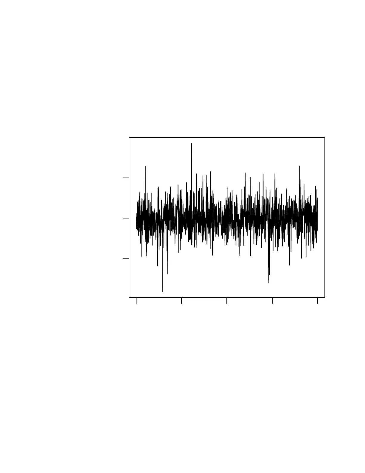
The Remark able Simplicit y of V ery High Dimensional Data: Application of Mo del-Based Clustering Fionn Murtagh ∗ Octob er 29, 2018 Abstract An ultrametric top ology formalizes the notion of hierarc hical structure. An ultrametric em b edding, referred to here as ultrametricity , is implied b y a hierarc hical em bedding. Suc h hierarc hical structure can b e global in the data set, or lo cal. By quantifying exten t or degree of ultrametricity in a data set, w e show that ultrametricity becomes perv asive as dimension- alit y and/or spatial sparsit y increases. This leads us to assert that v ery high dimensional data are of simple structure. W e exemplify this finding through a range of sim ulated data cases. W e discuss also application to v ery high frequency time series segmentation and mo deling. Keyw ords: multiv ariate data analysis, cluster analysis, hierarc hy , ultrametric, p-adic, dimensionality 1 In tro duction The lessons w e will draw from this w ork are as follo ws. • V ery high dimensional spaces are of very simple structure. • It b ecomes easier to find clusters in high dimensions. • The simple high dimensional structure is hierarchical. • Ease of handling high dimensional data, e.g. reading off clusters, em u- lates the human perception system which similarly pro cesses data with no eviden t latency . ∗ Department of Computer Science, Roy al Hollow ay , Universit y of London, Egham TW20 0EX, England. fmurtagh@acm.org 1 There is a burgeoning crisis in high dimensional data analysis, and man y curren t approaches lac k convincing performance guarantees. In Hinneburg, Ag- garw al and Keim (2000), atten tion is fo cused on “relev ant” dimensions only , while Aggarwal, Hinneburg and Keim (2001) (cf. the revealing titles in the case of b oth of these citations) state: “Recen t research results show that in high dimensional space, the concept of pro ximit y , distance or nearest neighbor may not ev en b e qualitativ ely meaningful.” The last-men tioned work in v estigates L p norms including for fractional v alues of p . In Breuel (2007), the fo cus is the  -appro ximate nearest neighbor defined as follows: if the nearest neigh b or p oint y to some query p oint, x , has distance d ( x, y ), then an y vector y 0 suc h that d ( y 0 , x ) ≤ (1 +  ) d ( x, y ) is an  -appro ximate nearest neighbor of x . Then Breuel (2007) p oin ts out: “... the relationship b e- t ween approximation and ’cost’ of a solution need not b e linear. F or example, the cost of picking an  -appro ximate nearest neighbor could b e prop ortional not to the difference of distances b et ween the optimal answer and the approxima- tion, but to the v olume of the shell b et ween the tw o, that is, as (1 +  ) m − 1 , where m is the dimension of the space.” V arious issues immediately ensue: (i) “for large dimensions, even small v alues of  include the en tire database as  - appro ximate neighbors”; (ii) “analyzing the worst-case asymptotic complexity of  -approximate algorithms is meaningless”; (iii) for “large enough dimensions, a randomly c hosen p oin t b ecomes an  -approximate nearest neighbor with high probabilit y”; (iv) “the implicit assumption that a close approximation leads to only a small increase in the cost of a solution is not justifiable in the context of nearest neighbors”; and (v) an  -approximate nearest neighbor algorithm is not necessarily useless in practice but such an algorithm has “neither useful mean- ing asymptotically (as the dimension gro ws), nor does it mak e useful predictions ab out its b eha vior on practical problems”. In this article, we prop ose an approac h which w e consider appropriate for high dimensional data analysis, based on clustering and pro ximity searching. 1.1 The Ultrametricity P ersp ectiv e and Ov erview of this W ork The morphology or inheren t shap e and form of an ob ject is imp ortan t. In data analysis, the inherent form and structure of data clouds are imp ortant. So the em b edding top ology , with which the data clouds are studied, can b e crucial. Quite a few mo dels of data form and structure are used in data analysis. One of them is a hierarchically embedded set of clusters, – a hierarch y . It is traditional (since at least the 1960s) to imp ose suc h a form on data, and if useful to assess the go odness of fit. Rather than fitting a hierarc hical structure to data (e.g., Rohlf and Fisher, 1968), our recen t work has taken a different orientation: we seek to find (partial or global) inherent hierarc hical structure in data. As w e will describ e in this article, there are in teresting findings that result from this, and some very in teresting p erspectives are op ened up for data analysis and, p o- ten tially , p erspectives also on the physics (or causal or generative mec hanisms) underlying the data. 2 A formal definition of hierarc hical structure is provided b y ultrametric top ol- ogy (in turn, related closely to p-adic num ber theory). W e will return to this in section 2 b elo w. First, though, we will summarize some of our findings. Ultrametricit y is a p erv asive prop erty of observ ational data. It arises as a limit case when data dimensionalit y or sparsit y gro ws. More strictly suc h a limit case is a regular lattice structure and ultrametricity is one possible represen- tation for it. Notwithstanding alternative representations, ultrametricity offers computational efficiency (related to tree depth/heigh t being logarithmic in n um- b er of terminal no des), link age with dynamical or related functional prop erties (ph ylogenetic interpretation), and pro cessing to ols based on well kno wn p-adic or ultrametric theory (examples: deriving a partition, or applying an ultramet- ric wa v elet transform). In Khrenniko v (1997) and other w orks, Khrenniko v has p oin ted to the imp ortance of ultrametric top ological analysis. Lo cal ultrametricit y is also of importance. This can be used for forensic data exploration (fingerprin ting data sets): see Murtagh (2005, 2007); and to exp e- dite search and discov ery in information spaces: see Ch´ av ez, Na v arro, Baeza- Y ates and Marroqu ´ ın (2001) as discussed by us in Murtagh (2004, 2006) and Murtagh, Downs and Contreras (2007). In section 2 w e sho w ho w exten t of ultrametricity is measured. Section 3 presen ts our main results on the remark able properties of v ery high dimensional, or very sparse, spaces. As dimensionality or sparsity grow, so do es the inher- en t hierarchical nature of the data in the space. In section 4 w e then discuss application to very high frequency time series mo deling. 1.2 Review of Recent Asymptotic Statistical Findings W e can characterize clustering algorithms in terms of num b er of observ ables, n , and num b er of attributes, m , where by “large” is meant thousands upw ards: (i) large n , small m ; as is fairly standard in astronomy; (ii) large n , large m ; as is fairly typically the case in information retriev al; and (iii) small n , large m ; as is often the case in bioinformatics, and textual forensics. It is case (iii) which is of most interest to us here. How ever our results also accommo date case (ii). In Hall, Marron and Neeman (2005), it was shown that “under some con- ditions on underlying distributions, as the dimension tends to infinity with a fixed sample size, the n data v ectors form a regular n -simplex in R m ” (Ahn, Marron, Muller and Chi, 2007). These authors term the small n , large m case “HDLSS, high dimension, low sample size”. In Ahn and Marron (2005), some other unrelated work is cited, where the ratio of m/n tends to a constant. As with these authors, our goal is to study the case of letting “ m tend to infinity , fixing n ” (Ahn and Marron, 2005). Hall et al. (2005) discuss previous asymp- totics work in the statistical literature. Our focus is not on a simplex but rather on a hierarch y (even if trivial) in order to study implications for data analysis. F or “the asymptotic geometric represen tation of HDLSS data”, it is sho wn in the w ork of Ahn and collab orators that “when m >> n , under a mild assump- tion, the pairwise distances b et w een each pair of data p oin ts are approximately iden tical so that the data p oin ts form a regular n -simplex. In a binary classifi- 3 cation setting, the training data from each class b ecomes tw o simplices ... an y reasonable classification metho d will find the same [discriminan t result] when m b ecomes very large.” (Ahn et al., 2007). This is a very exciting for the discriminan t analysis case pursued by Ahn et al., 2007; Ahn and Marron, 2005; Hall et al., 2005) (naive Bay es, SVM or supp ort vector machine, Fisher’s linear discriminan t, and the simplex structure in very high dimensions leading to the “direction of maximal data piling”). In this pap er, our in terest is in clustering, or unsup ervised classification. The mild condition for simplex structure formation, as m − → ∞ is that directionalit y of the Gaussian cloud is “diffuse”, defined in terms of eigen v alues: m X j λ 2 j /   m X j λ j   2 − → 0 as m − → ∞ Then it is sho wn that the co v ariance matrix approaches a constan t times the iden tity matrix. In Donoho and T anner (2005), the Gaussian case is also fo cused on. F or a Gaussian cloud, “not only are the p oints on the conv ex hull, but all reasonable- sized subsets span faces of the conv ex h ull”. Intuitiv ely , if all p oin ts fly apart from one another as dimensionality grows, then (i) eac h p oint is a vertex of the con vex h ull of the cloud of p oin ts; (ii) each pair of points generates an edge of the conv ex h ull; and (iii) sets of p oin ts form a regional face of the conv ex h ull. These prop erties are prov en by Donoho and T anner (2005) who conclude: “This is wildly differen t than the behavior that w ould be expected b y traditional lo w-dimensional thinking.” W e may ask why we (in this work ) lay imp ortance on the fact that the high dimensional simplex additionally defines an ultrametric top ological embedding. An ultrametric top ology requires (as will b e describ ed in sections to follo w) an y triangle to b e either (i) equilateral, or (ii) isosceles with small base. The equilateral case corresp onds fine with the simplex structure. But it is useful to us to hang on to the isosceles with small base case, to o, for inter-cluster relationships. W e will lo ok later at examples to supp ort this viewp oin t. 2 Quan tifying Degree of Ultrametricit y Summarizing a full description in Murtagh (2004) we explored tw o measures quan tifying how ultrametric a data set is, – Lerman’s and a new approac h based on triangle inv ariance (resp ectiv ely , the second and third approaches describ ed in this section). The triangular inequality holds for a metric space: d ( x, z ) ≤ d ( x, y ) + d ( y, z ) for any triplet of p oints x, y , z . In addition the prop erties of symmetry and p ositiv e definiteness are resp ected. The “strong triangular inequality” or ul- trametric inequality is: d ( x, z ) ≤ max { d ( x, y ) , d ( y , z ) } for any triplet x, y , z . An ultrametric space implies resp ect for a range of stringen t prop erties. F or 4 example, the triangle formed by an y triplet is necessarily isosceles, with the t wo large sides equal; or is equilateral. • Firstly , Rammal, T oulouse and Virasoro (1986) used discrepancy b et w een eac h pairwise distance and the corresp onding subdominant ultrametric. No w, the sub dominan t ultrametric is also known as the ultrametric dis- tance resulting from the single link age agglomerative hierarchical cluster- ing metho d. Closely related graph structures include the minimal span- ning tree, and graph (connected) comp onen ts. While the sub dominan t pro vides a go o d fit to the given distance (or indeed dissimilarity), it suf- fers from the “friends of friends” or chaining effect. • Secondly , Lerman (1981) developed a measure of ultrametricit y , termed H-classifiabilit y , using ranks of all pairwise given distances (or dissimilar- ities). The isosceles (with small base) or equilateral requirements of the ultrametric inequality imp ose constraints on the ranks. The in terv al b e- t ween median and maximum rank of every set of triplets must b e empty for ultrametricity . W e hav e used extensively Lerman’s measure of degree of ultrametricit y in a data set. T aking ranks provides scale in v ariance. But the limitation of Lerman’s approach, w e find, is that it is not reason- able to study ranks of real-v alued (v alues in non-negative reals) distances defined on a large set of p oin ts. • Thirdly , our o wn measure of extent of ultrametricity (Murtagh, 2004) can b e describ ed algorithmically . W e examine triplets of p oints (exhaustiv ely if possible, or otherwise through sampling), and determine the three angles formed by the asso ciated triangle. W e select the smallest angle formed by the triplet p oin ts. Then w e chec k if the other t wo remaining angles are appro ximately equal. If they are equal then our triangle is isosceles with small base, or equilateral (when all triangles are equal). The approxima- tion to equality is given b y 2 degrees (0.0349 radians). Our motiv ation for the approximate (“fuzzy”) equality is that it makes our approach robust and indep endent of measurement precision. A supposition for use of our measure of ultrametricity is that we can de- fine angles (and hence triangle prop erties). This in turn presupp oses a scalar pro duct. Thus we presuppose a complete normed vector space with a scalar pro duct – as one example, the real part of a Hilb ert space – to provide our needed environmen t. Quite a general wa y to em b ed data, to b e analyzed, in a Euclidean space, is to use c orrespondence analysis (Murtagh, 2005). This explains our in terest in using corresp ondence analysis: it provides a con venien t and versatile wa y to tak e input data in many v aried formats (e.g., ranks or scores, presence/absence, frequency of o ccurrence, and many other forms of data) and map them in to a Euclidean, factor space. 5 3 Ultrametricit y and Dimensionalit y 3.1 Distance Prop erties in V ery Sparse Spaces Murtagh (2004), and earlier work by Rammal, Angles d’Auriac and Doucot (1985) and Rammal et al. (1986), has demonstrated the p erv asiveness of ultra- metricit y , b y fo cusing on the fact that sparse high-dimensional data tend to b e ultrametric. In suc h work it is shown how num b ers of p oin ts in our clouds of data points are irrelev ant; but what coun ts is the ambien t spatial dimensionalit y . Among cases looked at are statistically uniformly (hence “unclustered”, or with- out structure in a certain sense) distributed p oin ts, and statistically uniformly distributed hypercub e v ertices (so the latter are random 0/1 v alued vectors). Using our ultrametricity measure, there is a clear tendency to ultrametricity as the spatial dimensionality (hence spatial sparseness) increases. As Hall et al. (2005) also show, Gaussian data b eha ve in the same wa y and a demonstration of this is seen in T able 1. T o provide an idea of consensus of these results, the 200,000-dimensional Gaussian was repeated and yielded on successiv e runs v alues of the ultrametricity measure of: 0.96, 0.98, 0.96. In the following, w e explain wh y high dimensional and/or sparsely populated spaces are ultrametric. W e use the Euclidean distances in the cosine formula to determine angles. Note that there is no av eraging of distances inv olved, nor distances normalized by dimensionality . As dimensionality gro ws, so to o do distances (or indeed dissimilarities, if they do not satisfy the triangular inequality). The least change possible for dissimilarities to b ecome distances has b een formulated in terms of the smallest additiv e constant needed, to b e added to all dissimilarities (T orgerson, 1958; Cailliez and Pag ` es, 1976; Cailliez, 1983; Neuwirth and Reisinger, 1982; and the comprehensiv e review of B´ enass´ eni, Bennani Dosse and Joly , 2007). Adding a sufficien tly large constant to all dissimilarities transforms them into a set of distances. Through addition of a larger constan t, it follo ws that distances b ecome approximately equal, th us verifying a trivial case of the ultrametric or “strong triangular” inequality . Adding to dissimilarities or distances may b e a direct consequence of increased dimensionality . F or a close fit or go od approximation, the situation is not as simple for taking dissimilarities, or distances, in to ultrametric distances. A best fit solution is given by de Soete (1986) (and softw are is av ailable in Hornik, 2005). If w e wan t a close fit to the given dissimilarities then a go o d choice would av ail either of the maximal inferior, or subdominant, ultrametric; or the minimal sup erior ultrametric. Stepwise algorithms for these are commonly known as, resp ectiv ely , single link age hierarc hical clustering; and complete link hierarchical clustering. (See Benz ´ ecri, 1979; Lerman, 1981; Murtagh, 1985; and other texts on hierarchical clustering.) 6 No. p oin ts Dimen. Isosc. Equil. UM Uniform 100 20 0.10 0.03 0.13 100 200 0.16 0.20 0.36 100 2000 0.01 0.83 0.84 100 20000 0 0.94 0.94 Hyp ercube 100 20 0.14 0.02 0.16 100 200 0.16 0.21 0.36 100 2000 0.01 0.86 0.87 100 20000 0 0.96 0.96 Gaussian 100 20 0.12 0.01 0.13 100 200 0.23 0.14 0.36 100 2000 0.04 0.77 0.80 100 20000 0 0.98 0.98 T able 1: Typical results, based on 300 sampled triangles from triplets of p oin ts. F or uniform, the data are generated on [0, 1]; h yp ercub e v ertices are in { 0 , 1 } m , and for Gaussian, the data are of mean 0, and v ariance 1. Dimen. is the am bient dimensionalit y . Isosc. is the num b er of isosceles triangles with small base, as a prop ortion of all triangles sampled. Equil. is the n umber of equilateral triangles as a prop ortion of triangles sampled. UM is the prop ortion of ultrametricit y- resp ecting triangles (= 1 for all ultrametric). 7 3.2 No “Curse of Dimensionalit y” in V ery High Dimen- sions Bellman’s (1961) “curse of dimensionality” relates to exp onential growth of h yp erv olume as a function of dimensionalit y . Problems b ecome tougher as di- mensionalit y increases. In particular problems related to proximit y search in high-dimensional spaces tend to b ecome intractable. In a w ay , a “trivial limit” (T rev es, 1997) case is reac hed as dimensionalit y in- creases. This mak es high dimensional proximit y search v ery different, and giv en an appropriate data structure – such as a binary hierarchical clustering tree – we can find nearest neighbors in worst case O (1) or constant computational time (Murtagh, 2004). The pro of is simple: the tree data structure affords a constan t num b er of edge trav ersals. The fact that limit prop erties are “trivial” makes them no less in teresting to study . Let us refer to such “trivial” prop erties as (structural or geometrical) regularit y prop erties (e.g. all p oin ts lie on a regular lattice). First of all, the symmetries of regular structures in our data may b e of imp ortance. F or example, pro cessing of such data can exploit these regularities. Secondly , “islands” or clusters in our data, where each “island” is of regular structure, may b e of interpretational v alue. Thirdly , and finally , regularity of particular prop erties do es not imply regu- larit y of all prop erties. So, for example, we may hav e only partial existence of pairwise link ages. Th us we see that in very high dimensions, and/or in very (spatially) sparse data clouds, there is a simplification of structure, whic h can b e used to mitigate an y “curse of dimensionalit y”. Figure 1 shows how the distances within and b et w een clusters b ecome tighter with increase in dimensionality . 3.3 Gaussian Clusters in V ery High Dimensions 3.3.1 In tro duction W e will distinguish b etw een cluster characteristics as follows: 1. cluster size: n umber of p oin ts p er cluster; 2. cluster lo cation: here, mean, iden tical on every dimension; 3. cluster scale: here, standard deviation, identical on every dimension. These cluster characteristics are simple ones which serve to exemplify how high dimensional clustering is quite different from analogous problems in low dimensions. In the homogeneous clouds studied in T able 1 it is seen that the isosceles (with small base) case disappeared early on, as dimensionality increased greatly , to the adv an tage of the equilateral case of ultrametricity . So the p oin ts b ecome increasingly equilateral-related as dimensionality grows. This is not the case when the data in clustered, as we will now see. 8 Dim 2000 3 sets of 100 pts, mean 0, var 1, 3, 7 Frequency 100 200 300 400 0 1500 Dim 20000 3 sets of 100 pts, mean 0, var 1, 3, 7 Frequency 200 400 600 800 1000 1200 1400 0 5000 Figure 1: An illustration of how “symmetry” or “structure” can b ecome in- creasingly pronounced as dimensionality increases. The abscissa sho ws distance v alues. Display ed are t wo sim ulations, eac h with 3 sub-populations of Gaussian- distributed data, in, respectively , am bien t dimensions of 2000 and 20,000. These sim ulations corresp ond to the 3rd last, and 2nd last, rows of T able 1. 9 No. p oin ts Dimen. Isosc. Equil. UM 200 20 0.08 0 0.08 200 200 0.19 0.04 0.23 200 2000 0.42 0.20 0.62 200 20000 0.74 0.22 0.96 200 20000 0.7 0.28 0.98 200 20000 0.77 0.21 0.98 200 20000 0.76 0.21 0.98 200 20000 0.75 0.24 0.99 200 20000 0.73 0.25 0.98 T able 2: Results based on 300 sampled triangles from triplets of p oin ts. Two Gaussian clusters, eac h of 100 points, w ere used in eac h case. One point set w as of mean 0, and the other of mean 10, on eac h dimension. The standard deviations on eac h dimension were 1 in all cases. Column headings are as in T able 1. Fiv e further results are giv en for the 20,000-dimension case to show v ariabilit y . 3.3.2 Clusters with Different Lo cations, Same Scale T able 2 is based on tw o clusters, and sho ws how isosceles triangles increasingly dominate as dimensionality grows. Figure 2 illustrates low and high dimension- alit y scenarios relating to T able 2. There is clear confirmation in this table as to how in terrelationships in the cluster b ecome more compact and, in a certain sense, more trivial, in high dimensions. This do es not obscure the fact that w e indeed hav e hierarchial relationships b ecoming ever more pronounced as di- mensionalit y , and hence relative sparsity , increase. These observ ations help us to see quite clearly just how hierachical relationships come ab out, as ambien t dimensionalit y grows. 3.3.3 Clusters with Different Lo cations, Different Scales A more demanding case study is now tried. W e generate 50 p oin ts p er cluster with the following c haracteristics: mean 0, standard deviation 1, on each di- mension; mean 3, standard deviation 2, on each dimension; mean 5, standard deviation 1, on each dimension; and mean 8, standard deviation 3, on eac h di- mension. T able 3 sho ws the results obtained. Here we hav e not achiev ed quite the same level of ultrametricty , due to slow er growth in ultrametricit y which is, in turn, due to the more murky , less dermarcated, but undoubtdely clustered, set of data. Figure 3 illustrates this: this histogram shows one dimension (i.e., one co ordinate, chosen arbitrarily), where w e note that means of the Gaussians are at 0, 3, 5 and 8. When we look closer at T able 3, as shown in Figure 4, the compaction of 10 100+100 x 20 Distances Frequency 10 20 30 40 50 0 1500 100+100 x 20000 Distances Frequency 200 400 600 800 1000 1200 1400 0 6000 Figure 2: A further illustration of how “symmetry” or “structure” can b ecome increasingly pronounced as dimensionality increases, relating to the 200 × 20 and 200 × 20 , 000 (first of the succession of rows) cases of T able 2. These are histograms of all interpoint distances, based on tw o Gaussian clusters. The first has mean 0 and standard deviation 1 on all dimensions. The second has mean 10 and standard deviation 1 on all dimensions. 11 Projection on one dimension Positions Frequency 0 5 10 0 2 4 6 8 Figure 3: A pro jection on to one dimension, to illustrate the less than clearcut clustering problem addressed. There are four Gaussians here, each of 50 real- izations, with means at 0, 3, 5 and 8, and with resp ectiv e standard deviations of 1, 2, 1, 3. 12 No. p oin ts Dimen. Isosc. Equil. UM 200 20 0.04 0.01 0.05 200 200 0.11 0.05 0.16 200 2000 0.28 0.06 0.34 200 20000 0.5 0.08 0.58 200 200000 0.55 0.11 0.66 T able 3: Results based on 300 sampled triangles from triplets of p oints. F our Gaussian clusters, each of 50 p oin ts, were used in each case. See text for details of prop erties of these clusters. distances is again very interesting. W e verified the 7 p eaks found in the low er histogram in Figure 4, and av ailable but confusedly ov erlapping and ill-defined in the upp er histogram of Figure 4. What w e find for the 7 p eaks is as follows. Distances within the clusters corresp ond to: p eaks 1, 2, 3 and (again) 1. That tw o clusters are associated with one p eak is clear from the fact that tw o of our clusters are of identical scale. W e can examine inter-cluster distances and we found these to b e asso ciated with p eaks: 2, 3, 4, 5, 6, 7. Giv en 4 clusters, we could w ell hav e up to 6 p ossible additional p eaks. W ere we to b e in a far higher dimensional am bient space then we could exp ect even the inter-cluster distances to b ecome equi-distant. 3.3.4 Iden tifiability of High Dimensional Gaussian Clouds F rom these case studies, it is clear that increased dimensionality sharp ens and distinguishes the clusters. If w e can embed data – any data – in a far higher am bient dimensionality , without destroying the interpretable relationships in the data, then we can so muc h more easily read off the clusters. T o read off clusters, including mem b erships and prop erties, our findings can b e summarized as follows. F or cluster size (i.e., num b ers of p oints p er cluster), sampling alone can b e used, and we do not pursue this here. F or cluster scale (i.e., standard deviation, assumed the same on eac h di- mension), we asso ciate each cluster, or a pair of clusters, with each p eak. The total num ber of p eaks gives an upp er b ound on the num b er of clusters. (F or k clusters, we hav e ≤ k + k · ( k − 1) / 2 p eaks.) Using cluster scale also p ermits use of the following cluster mo del: supp ose that all clusters are defined to ha ve in tra-cluster distance that is less than inter- cluster distance. Then it follows that the p eaks of low er distance corresp ond to the clusters (as opp osed to pairs of clusters). An example of this is as follows. In Figure 4, low er panel, we read from left to right, applying the follo wing algorithm: se lect the first k p eaks as clusters, 13 4 clusters x 20 Distances Frequency 10 20 30 40 0 400 4 clusters x 200000 Distances Frequency 500 1000 1500 2000 2500 3000 3500 4000 0 2000 Figure 4: Compaction of distances with rise in dimensionalit y: 4 clusters, sub- stan tially ov erlapping are the basis for the histograms of all pairwise distances. T op: ambien t dimensionality 20. Bottom: ambien t dimensionality 200,000. 14 90 points, 3 clusters, dim. 1000 Distances Frequency 0 200 400 600 800 1000 1200 0 150 350 90 points, 3 clusters, dim. 10000 Distances Frequency 0 1000 2000 3000 4000 0 300 Figure 5: Histogram of interpoint distances. Three homogeneous clusters, each of 30 p oin ts, in spaces of dimensions 1000 and 10000. and ask: are there sufficien t p eaks to represent all in ter-cluster pairs? If we c ho ose k = 3, there remain 4 p eaks, which is to o many to account for the inter- cluster pairs (i.e., 3 · (3 − 1) / 2)). So we see that Figure 4 is incompatible with k = 3 or the presence of just 3 clusters. Consequen tly w e mo ve to k = 4, and see that Figure 4 is consistent with this. A further identifiabilit y assumption is reasonable alb eit not required: that all smallest p eaks b e asso ciated with in tra-cluster distances. This need not b e so, since w e could w ell ha ve a dense cluster sup erimposed on a less dense one. How ever it is a reasonable parsimony assumption. Supported by this assumption, Figure 4 p oin ts to a minim um of 4 clusters in the data, with up to 4 p eaks (read off from left to right, i.e., in increasing order of distance) corresp onding to these clusters. Figure 5 sho ws p eaks, sharp ening with rise in am bient dimensionality , for three clusters, distributed as Gaussians with resp ectiv ely means and standard deviations on all dimensions: (10, 0.5); (0, 4); (40, 10). W e see the p eaks 15 120 points, 4 clusters, dim. 1000 Distances Frequency 0 200 400 600 800 1000 1200 0 200 120 points, 4 clusters, dim. 10000 Distances Frequency 0 1000 2000 3000 4000 0 400 Figure 6: Histogram of interpoint distances. F our homogeneous clusters, each of 30 p oin ts, in spaces of dimensions 1000 and 10000. 16 240 points, 4 double clusters, dim. 1000 Distances Frequency 0 200 400 600 800 1000 1200 1400 0 600 240 points, 4 double clusters, dim. 10000 Distances Frequency 0 1000 2000 3000 4000 0 1000 Figure 7: Histogram of interpoint distances. F our heterogeneous clusters, each of 60 p oints (comprising tw o subgroups of 30 p oin ts each), in spaces of dimen- sions 1000 and 10000. 17 corresp onding to the increasingly similar (and tending tow ards iden tical) intra- cluster distances; and then the peaks asso ciated with the 3 in ter-cluster distance sets: 6 p eaks in total. Figure 6 again shows p eaks for four clusters, with the same characteristics as for Figure 5, but with an additional cluster of mean and standard deviation on all co ordinates: (25, 7). Here we find, as exp ected, 4 intra-cluster distance p eaks, and 6 inter-cluster distance p eaks: 10 p eaks in total. The success of cluster identification is clearly dep enden t on distinguishable in tra-cluster prop erties, which are also distinguishable from the inter-cluster prop erties. Figure 7 shows a more tricky case. F or the first cluster, the (equally-sized comp onen t) distributions had means and standard deviations on all co ordinates of: (10, 0.5) and (0, 0.5). F or the second cluster, we used: (0, 4) and (10, 4). F or the third cluster we used (40, 10) and (0, 10). Finally for the fourth cluster w e used the same for all cluster member points: (25, 7). Here, therefore the maxim um n umber of p eaks is: for the intra-cluster distances, 2 p eaks for the first, second and third clusters, and 1 for the fourth cluster, hence 7. F or the in ter-cluster distances, assuming the cluster comp onents are close enough, 6, but if they are not, then, w e hav e p eaks b et ween essentially 7 clusters, i.e. 21 p eaks. Hence in total w e could ha v e up to 28 peaks. F or the histogram sampling resolution used, we read off, visually , 17 p eaks. Our approach is to hav e an upp er b ound on the num b er of p eaks found in the distance histogram. Now we turn to real (or realistic) data and see ho w this w ork helps us to address the cluster identifiabilit y problem. 4 Applications 4.1 Application to High F requency Data Analysis In this section we establish pro of of concept for application of the foregoing w ork to analysis of very high frequency univ ariate time series signals. Consider eac h of the cases considered in section 3.3, expressed there as n × m arra ys, as instead representing n segmen ts, each of (con tiguous) length m , of a time series or one-dimensional signal. Assuming our aim is to cluster these segmen ts on the basis of their prop erties, then it is reasonable to require that they b e non-ov erlapping. The n segmen ts could come from anywhere, in an y order, in the time series. So for the case of an n × m arra y considered previously , then implies a time series of length at least nm . The most immediate w ay to construct the time series is to raster scan the n × m array , although alternatives come readily to mind. The methodology discussed in section 3.3 then is seen to b e also a time series segmen tation approach, facilitating the characterizing of the segments used. T o explore this further w e consider a time series consisting of t wo ARIMA (autoregressiv e integrated moving a v erage) mo dels, with parameters: order, au- toregression co efficien ts, moving av erage co efficien ts, and a “mildly longtailed” 18 No. time series Dimen. Isosc. Equil. UM 100 2000 0.17 0.32 0.49 100 20000 0.15 0.5 0.65 100 200000 0.03 0.57 0.60 T able 4: Results based on 300 sampled triangles from triplets of p oin ts. Two sets of the ARIMA mo dels are used, each of 50 realizations. set of inno v ations based on the Studen t t distribution with 5 degrees of freedom. Figures 8 and 9 show samples of these time series segments. Figures 10 and 11 sho w histograms of these samples. T able 4 shows typical results obtained in regard to ultrametricity . The di- mensionalit y can b e considered as the embedding dimension. Here, although ultrametricit y increases, and the equilateral configuration seems to b e increas- ing but with decrease of the isosceles with small base configuration, we do not consider it of practical relev ance to test with even higher ambien t dimensional- ities. It is clear from the data, esp ecially Figures 10 and 11, that the tw o signal mo dels are v ery close in their prop erties. Examining the histograms of all inter-pair time series segments, b oth intra and in ter cluster, we find the clearly distinguished peaks shown in Figure 12. As b efore, we use Euclidean distance b etw een time series segments or v ectors. (W e note that normalization or other transformation is not relev ant here. In fact w e wan t to distinguish b et ween inter and intra cluster cases. F urthermore the un weigh ted Euclidean distance is consistent with our use of angles to quantify triangle inv arian ts, and hence resp ect for ultrametricity prop erties.) W e find clearly distinguishable p eaks in Figure 12. The lo wer and the higher p eaks b elong to the t wo ARIMA comp onen ts. The central p eak b elongs to the in ter-cluster distances. W e hav e shown that our metho dology can b e of use for time series segmen- tation and for mo del identifiabilit y . Given the use of a scalar pro duct space as the essential springb oard of all asp ects of this work, it would app ear that gen- eralization of this work to multiv ariate time series analysis is straightforw ard. What remains imp ortan t, how ever, is the av ailability of very large embedding dimensionalities, i.e. very high frequency data streams. 4.2 Application in Practice: Segmen ting a Financial Sig- nal W e use financial futures, circa Marc h 2007, denominated in euros from the D AX exc hange. Our data stream is at the millisecond rate, and comprises ab out 382,860 records. Each record includes: 5 bid and 5 asking prices, together with bid and asking sizes in all cases , and action. W e extracted one symbol (commo dit y) with 95,011 single bid v alues, on which w e no w report results. See 19 0 500 1000 1500 2000 −2 0 2 Time Value Figure 8: Sample (using first 2000 v alues) of a time series segment, based on the first ARIMA set of parameters. (Order 2 AR parameters: 0 . 8897 , − 0 . 4858, MA parameters: − 0 . 2279 , 0 . 2488.) 20 0 500 1000 1500 2000 −4 −2 0 2 Time Value Figure 9: Sample (using first 2000 v alues) of a time series segmen t, based on the second ARIMA set of parameters. (Order 2 AR parameters: 0 . 2897 , − 0 . 1858, MA parameters: − 0 . 7279 , 0 . 7488.) 21 1st ARIMA series (1000 values) Value Frequency −4 −2 0 2 4 0 20 40 60 80 100 120 Figure 10: Histogram of sample (using first 2000 v alues) of time series segment sho wn in Figure 8. 22 2nd ARIMA series (1000 values) Value Frequency −3 −2 −1 0 1 2 3 0 20 40 60 Figure 11: Histogram of sample (using first 2000 v alues) of time series segment sho wn in Figure 9. 23 100 segments, each of 200k values Distances Frequency 410 415 420 425 430 435 440 445 0 100 200 300 400 500 Figure 12: Histogram of distances from 100 time series segments, using 50 segmen ts each from the t wo ARIMA mo dels, and using an em b edding dimen- sionalit y of 200,000. 24 Figure 13. Em b eddings were defined as follows. • Windows of 100 successiv e v alues, starting at time steps: 1, 1000, 2000, 3000, 4000, . . . , 94000. • Windows of 1000 successive v alues, starting at time steps: 1, 1000, 2000, 3000, 4000, . . . , 94000. • Windows of 10000 successive v alues, starting at time steps: 1, 1000, 2000, 3000, 4000, . . . , 85000. The histograms of distances b et ween these windows, or embeddings, in re- sp ectiv ely spaces of dimension 100, 1000 and 10000, are shown in Figure 14. Note how the 10000-length windo w case results in p oin ts that are strongly o verlapping. In fact, we can say that 90% of the v alues in eac h window are o verlapping with the next window. Not withstanding this ma jor ov erlapping in regard to clusters inv olved in the pairwise distances, if we can still find clusters in the data then w e ha ve a v ery v ersatile w ay of tac kling the clustering ob jectiv e. Because of the greater cluster concentration that we exp ect (from discussion in earlier sections of this article) from a greater em b edding dimension, we use the 86 p oin ts in 10000-dimensional space, not withstanding the fact that these points are from ov erlapping clusters. W e make the follo wing supp osition based on Figure 13: the clusters will consist of successive v alues, and hence will b e justifiably termed segments. T o v alidate our approac h we will pursue three separate attacks on the same problem of time series segmen tation. Firstly , from the distances histogram in Figure 14, bottom, we will carry out Gaussian mixture modeling follo wed b y use of the Bay esian information criterion (BIC, Sc hw arz, 1978) as an approximate Ba yes factor, to determine the b est n umber of clusters (effectively , histogram p eaks). Secondly we will use an adjacency-resp ecting hierarchical clustering algorithm on the full-dimensional (viz., 10000) data. Thirdly , we will use a reduced dimensionalit y mapping, principal coordinates analysis, using the in ter- p oin t distances. Our assumptions in regard to what clusters are present in the data are minimal. F urthermore our v alidation of segmen ts is based on the three differen t wa ys that w e hav e of tac kling the one segmentation problem. W e fit a Gaussian mixture model to the data sho wn in the b ottom histogram of Figure 14. T o derive the appropriate num b er of histogram peaks w e fit Gaussians and use the Bay esian information criterion (BIC) as an approximate Ba yes factor for mo del selection (Kass and Raftery , 1995; Murtagh and Starck, 2003). Figure 15 shows the succession of outcomes, and indicates as b est a 5-Gaussian fit. F or this result, we find the means of the Gaussians to b e as follo ws: 517, 885, 1374, 2273 and 3908. The corresp onding standard deviations are: 84, 133, 212, 410 and 663. The resp ectiv e cardinalities of the 5 histogram p eaks are: 358, 1010, 1026, 911 and 350. Note that this relates so far only to the histogram of pairwise distances. W e now wan t to determine the corresp onding clusters in the input data. 25 0 20000 40000 60000 80000 6790 6810 6830 6850 Time steps Bid price Figure 13: The signal used: a commodity future, with millisecond time sam- pling. 26 Dim. 100 0 100 200 300 400 500 600 0 250 Dim. 1000 0 500 1000 1500 2000 0 300 Dim. 10000 0 1000 2000 3000 4000 5000 6000 0 200 Figure 14: Histograms of pairwise distances b et ween embeddings in dimension- alities 100, 1000, 10000. Resp ectiv ely the num b ers of embeddings are: 95, 95 and 86. 27 2 4 6 8 10 −39000 −38500 −38000 −37500 Number of Gaussians BIC value Figure 15: BIC (Bay esian information criterion) v alues for the succession of results. The 5-cluster solution has the highest v alue for BIC and is therefore the b est Gaussian mixture fit. 28 While we hav e the segmentation of the distance histogram, we need the seg- men tation of the original financial signal. If we had 2 clusters in the original financial signal, then we could exp ect up to 3 p eaks in the distances histogram (viz., 2 intra-cluster p eaks, and 1 in ter-cluster peak). If w e had 3 clusters in the original financial signal, then we could exp ect up to 6 p eaks in the dis- tances histogram (viz., 3 intra-cluster p eaks, and 3 inter-cluster p eaks). This information is consistent with asserting that the evidence from Figure 15 p oin ts to tw o of these histogram p eaks b eing approximately co-lo cated (alternatively: the distances are approximately the same). W e conclude that 3 clusters in the original financial signal is the most consistent num b er of clusters. W e will now determine these. One possibility is to use principal coordinates analysis (T orgerson’s, Gow er’s metric multidimensional scaling) of the pairwise distances. In fact, a 2-dimensional mapping furnishes a very similar pairwise distance histogram to that seen using the full, 10000, dimensionality . The first axis in Figure 16 accounts for 88.4% of the v ariance, and the second for 5.8%. Note therefore how the scales of the planar representation in Figure 16 p oin t to it b eing very linear. Benz ´ ecri (1979, V ol. I I, chapter 7, section 3.1) discusses the Guttman effect, or Guttman scale, where factors that are not mutually correlated, are nonethe- less functionally related. When there is a “fundamen tally unidimensional un- derlying phenomenon” (there are m ultiple such cases here) factors are functions of Legendre polynomials. W e can view Figure 16 as consisting of m ultiple horse- sho e shapes. A simple explanation for suc h shap es is in terms of the constraints imp osed by lots of equal distances when the data vectors are ordered linearly: see Murtagh (2005, pp. 46-47). Another view of how embedded (hence clustered) data are capable of b eing w ell mapp ed in to a unidimensional curv e is Critc hley and Heiser (1988). Critc h- ley and Heiser show one approach to mapping an ultrametric into a linearly or totally ordered metric. W e hav e asserted and then established ho w hierarch y in some form is relev an t for high dimensional data spaces; and then we find a very linear pro jection in Figure 16. As a consequence we note that the Critchley and Heiser result is esp ecially relev ant for high dimensional data analysis. Kno wing that 3 clusters in the original signal are wan ted, we will use an adjacency-constrained agglomerative hierarchical clustering algorithm to find them: see Figure 17. The contiguit y-constrained complete link criterion is our only choice here if we are to b e sure that no inv ersions can come ab out in the hierarc hy , as explained in Murtagh (1985). As input, w e use the co ordinates in Figure 16. The 2-dimensional Figure 16 representation relates to ov er 94% of the v ariance. The most complete basis w as of dimensionality 85. W e chec ked the results of the 85-dimensionalit y em b edding whic h, as noted below, ga ve v ery similar results. Reading off the 3-cluster mem b erships from Figure 17 gives for the signal actually used (with a v ery initial segmen t and a very final segment deleted): cluster 1 corresp onds to signal v alues 1000 to 33999 (p oints 1 to 33 in Figure 17); cluster 2 corresp onds to signal v alues 34000 to 74999 (p oints 34 to 74 in Figure 17); and cluster 3 corresp onds to signal v alues 75000 to 86999 (points 29 −2000 −1000 0 1000 2000 3000 −600 −400 −200 0 200 400 600 Principal coordinate 1 Principal coordinate 2 1 2 3 4 5 6 7 8 9 10 11 12 13 14 15 16 17 18 19 20 21 22 23 24 25 26 27 28 29 30 31 32 33 34 35 36 37 38 39 40 41 42 43 44 45 46 47 48 49 50 51 52 53 54 55 56 57 58 59 60 61 62 63 64 65 66 67 68 69 70 71 72 73 74 75 76 77 78 79 80 81 82 83 84 85 86 Figure 16: An in teresting representation – a type of “return map” – found using a principal co ordinates analysis of the 86 successive 10000-dimensional p oin ts. Again a demonstration that v ery high dimensional structures can b e of v ery simple structure. The planar pro jection seen here represents most of the information conten t of the data: the first axis accounts for 88.4% of the v ariance, while the second accounts for 5.8%. 30 75 to 86 in Figure 17). This allows us to segment the original time series: see Figure 18. (The clustering of the 85-dimensional embedding differs minimally . Segmen ts are: p oin ts 1 to 32; 33 to 73; and 74 to 86.) T o summarize what has b een done: 1. the segmentation is initially guided by the p eak-finding in the histogram of distances 2. with high dimensionality we exp ect simple structure in a lo w dimensional mapping provided by principal co ordinates analysis 3. which we use as input to a sequence-constrained clustering m ethod in order to determine the clusters 4. which can then b e display ed on the original data. In this case, the clusters are defined using a complete link criterion, implying that these three clusters are determined by minimizing their maximum internal pairwise distance. This provides a strong measure of signal v olatility as an explanation for the clusters, in addition to their a verage v alue. 5 Conclusions One interesting conclusion on this work follows. T raditionally , clustering algo- rithms hav e generally b een considered as distance-based or mo del-based. The former is exemplified by agglomerative hierarchical clustering, or k-means par- titioning. The latter is exemplified by Gaussian mixture mo deling. (One moti- v ation for mo del-based clustering is the computational difficult y , in general, of taking account of all pairwise distances.) The approach describ ed in this work is b oth distance-based and mo del-based. What we hav e observed in all of this work is that in the limit of high di- mensionalit y a scalar pro duct space b ecomes ultrametric. It has b een our aim in this work to link observed data with an ultrametric top ology for such data. The traditional approach in data analysis, of course, is to imp ose structure on the data. This is done, for example, b y using some agglomerative hierarchical clustering algorithm. W e can alwa ys do this (mo dulo distance or other ties in the data). Then w e can assess the degree of fit of suc h a (tree or other) structure to our data. F or our purp oses, here, this is unsatisfactory . • Firstly , our aim was to show that ultrametricity can b e naturally present in our data, globally or lo cally . W e did not w ant an y “measuring to ol” suc h as an agglomerative hierarchical clustering algorithm to ov erly in- fluence this finding. (Unfortunately Rammal et al., 1986, suffers from precisely this unhelpful influence of the “measuring to ol” of the sub dom- inan t ultrametric. In other resp ects, Rammal et al., 1986, is a seminal pap er.) 31 0 1000 2000 3000 4000 5000 1 2 3 4 5 6 7 8 9 10 11 12 13 14 15 16 17 18 19 20 21 22 23 24 25 26 27 28 29 30 31 32 33 34 35 36 37 38 39 40 41 42 43 44 45 46 47 48 49 50 51 52 53 54 55 56 57 58 59 60 61 62 63 64 65 66 67 68 69 70 71 72 73 74 75 76 77 78 79 80 81 82 83 84 85 86 Figure 17: Hierarchical clustering of the 86 p oints. Sequence is resp ected. The agglomerativ e criterion is the contiguit y-constrained complete link metho d. See Murtagh (1985) for details including pro of that there can b e no in version in this dendrogram. 32 0 20000 40000 60000 80000 6790 6800 6810 6820 6830 6840 6850 6860 Time steps Value Figure 18: Boundaries found for 3 segments. • Secondly , let us assume that we did use hierarchical clustering, and then based our discussion around the goo dness of fit. This again is a traditional approac h used in data analysis, and in statistical data modeling. But such a discussion would hav e b een unnecessary and futile. F or, after all, if we ha ve ultrametric prop erties in our data then many of the widely used hierarc hical clustering algorithms will give precisely the same outcome , and furthermore the fit is by definition optimal. (Our p oin t here is that if min { d ik | i ∈ q , k 6∈ q , k 6 = q } = max { d ik | i ∈ q , k 6∈ q , k 6 = q } for cluster q , at all agglomerations, then single link age and complete link age are iden tical.) W e hav e describ ed an application of this work to v ery high frequency signal pro cessing. The t win ob jectives are signal segmen tation, and mo del identifica- tion. W e ha ve noted that a considerable amount of this work is mo del-based: w e require assumptions (on clusters, and on mo del(s)) for identifiabilit y . Motiv ation for this work includes the a v ailability of very high frequency data streams in v arious fields (ph ysics, engineering, finance, meteorology , bio- engineering, and bio-medicine). By using a very large embedding dimensionalit y , w e are approaching the data analysis on a v ery gross scale, and hence furnishing a particular t yp e of m ultiresolution analysis. That this is w orthwhile has b een sho wn in our case studies. 33 References A GGAR W AL, C.C., HINNEBURG, A. and KEIM, D.A. (2001). “On the Sur- prising Behavior of Distance Metrics in High Dimensional Spaces”, Pr o c e e dings of the 8th International Confer enc e on Datab ase The ory , pp. 420–434, January 04-06. AHN, J., MARRON, J.S., MULLER, K.E. and CHI, Y.-Y. (2007). “The High Dimension, Lo w Sample Size Geometric Representation Holds under Mild Con- ditions”, Biometrika , 94, 760–766. AHN, J. and MARR ON, J.S. (2005). “Maximal Data Piling in Discrimination”, Biometrika , submitted; and “The Direction of Maximal Data Piling in High Dimensional Space”. BELLMAN, R. (1961). A daptive Contr ol Pr o c esses: A Guide d T our , Princeton Univ ersity Press. B ´ ENASS ´ ENI, J., BENNANI DOSSE, M. and JOL Y, S. (2007). On a General T ransformation Making a Dissimilarity Matrix Euclidean, Journal of Classifi- c ation , 24, 33–51. BENZ ´ ECRI, J.P . (1979). L’Analyse des Donn´ ees, T ome I T axinomie , T ome II Corr esp ondanc es , 2nd ed., Duno d, Paris. BREUEL, T.M. (2007). “A Note on Approximate Nearest Neighbor Metho ds”, h ttp://arxiv.org/p df/cs/0703101 CAILLIEZ, F. and P AG ` ES, J.P . (1976). Intr o duction ` a l’Analyse de Donn ´ ees , SMASH (So ci´ et ´ e de Math´ ematiques Appliqu ´ ees et de Sciences Humaines), P aris. CAILLIEZ, F. (1983). “The Analytical Solution of the Additiv e Constan t Prob- lem”, Psychometrika , 48, 305–308. CH ´ AVEZ, E., NA V ARRO, G., BAEZA-Y A TES, R. and MARROQU ´ IN, J.L. (2001). “Proximit y Searching in Metric Spaces”, ACM Computing Surveys , 33, 273–321. CRITCHLEY, F. and HEISER, W. (1988), “Hierarchical trees can b e p erfectly scaled in one dimension” Journal of Classific ation , 5, 5–20. DE SOETE, G. (1986). “A Least Squares Algorithm for Fitting an Ultrametric T ree to a Dissimilarity Matrix”, Pattern R e c o gnition L etters , 2, 133–137. DONOHO, D.L. and T ANNER, J. (2005). “Neighborliness of Randomly-Pro jected Simplices in High Dimensions”, Pr o c e e dings of the National A c ademy of Sci- enc es , 102, 9452–9457. HALL, P ., MARRON, J.S. and NEEMAN, A. (2005). “Geometric Representa- tion of High Dimension Low Sample Size Data”, Journal of the R oyal Statistic al So ciety B , 67, 427–444. HEISER, W.J. (2004). “Geometric Represen tation of Asso ciation b et ween Cat- egories”, Psychometrika , 69, 513–545. 34 HINNEBUR G, A., AGGAR W AL, C. and KEIM, D. (2000). “What is the Near- est Neigh b or in High Dimensional Spaces?”, VLDB 2000, Pr o c e e dings of 26th International Confer enc e on V ery L ar ge Data Bases , September 10-14, 2000, Cairo, Egypt, Morgan Kaufmann, pp. 506–515. HORNIK, K. (2005). “A CLUE for CLUster Ensem bles”, Journal of Statistic al Softwar e , 14 (12). KASS, R.E. and RAFTER Y, A.E. (1995). “Bay es F actors and Mo del Uncer- tain ty”, Journal of the Americ an Statistic al Asso ciation , 90, 773–795. KHRENNIK OV, A. (1997). Non-A r chime de an Analysis: Quantum Par adoxes, Dynamic al Systems and Biolo gic al Mo dels , Kluw er. LERMAN, I.C. (1981). Classific ation et Analyse Or dinale des Donn´ ees , Paris, Duno d. MUR T AGH, F. (1985). Multidimensional Clustering A lgorithms , Ph ysica-V erlag. MUR T AGH, F. (2004). “On Ultrametricit y , Data Co ding, and Computation”, Journal of Classific ation , 21, 167–184. MUR T AGH, F. (2005). “Iden tifying the Ultrametricit y of Time Series”, Eur o- p e an Physic al Journal B , 43, 573–579. MUR T AGH, F. (2007). “A Note on Lo cal Ultrametricity in T ext”, h ttp://arxiv.org/p df/cs.CL/0701181 MUR T AGH, F. (2005). Corr esp ondenc e Analysis and Data Co ding with R and Java , Chapman & Hall/CRC. MUR T AGH, F. (2006). “F rom Data to the Physics using Ultrametrics: New Results in High Dimensional Data Analysis”, in A.Y u. Khrennik ov, Z. Raki´ c and I.V. V olo vich, Eds., p-A dic Mathematic al Physics , American Institute of Ph ysics Conf. Pro c. V ol. 826, 151–161. MUR T AGH, F., DO WNS, G. and CONTRERAS, P . (2008). “Hierarchical Clus- tering of Massiv e, High Dimensional Data Sets by Exploiting Ultrametric Em- b edding”, SIAM Journal on Scientific Computing , 30, 707–730. MUR T AGH, F. and ST ARCK, J.L. (2003). “Quan tization from Ba yes F actors with Application to Multilevel Thresholding”, Pattern R e c o gnition L etters , 24, 2001–2007. NEUWIR TH, E. and REISINGER, L. (1982). “Dissimilarity and Distance Co- efficien ts in Automation-Supp orted Thesauri”, Information Systems , 7, 47–52. RAMMAL, R., ANGLES D’AURIA C, J.C. and DOUCOT, B. (1985). “On the Degree of Ultrametricity”, L e Journal de Physique – L ettr es , 46, L-945–L-952. RAMMAL, R., TOULOUSE, G. and VIRASORO, M.A. (1986). “Ultrametric- it y for Physicists”, R eviews of Mo dern Physics , 58, 765–788. R OHLF, F.J. and FISHER, D.R. (1968). “T ests for Hierarchical Structure in Random Data Sets”, Systematic Zo olo gy , 17, 407–412. 35 SCHW ARZ, G. (1978). “Estimating the Dimension of a Mo del”, Annals of Statistics , 6, 461–464. TOR GERSON, W.S. (1958). The ory and Metho ds of Sc aling , Wiley . TREVES, A. (1997). “On the Perceptual Structure of F ace Space”, BioSystems , 40, 189–196. 36