Quantum Theory, Noncommutativity and Heuristics

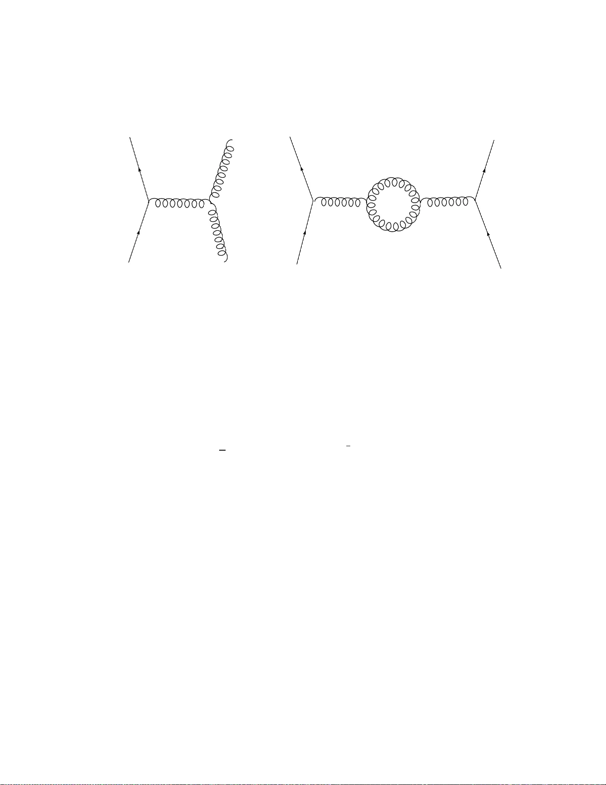
Quan tum Theory , Noncomm utativit y and Heuristics Earnest Ak ofor e akofor@physics.syr.e du Dep artment of Physics, Syr acuse University, Syr acuse, NY 13244 -1130, USA (h ttp://users.aims.ac.za/ ∼ ak ofor/academics/academics.h t ml ) Abstract Noncomm utativ e ﬁeld theories are a class of theories b ey ond the standard mo del of elemen tar y particle ph ysics. Th eir imp ortance may be summarized in tw o facts. Firstly as ﬁeld theories on noncomm utativ e spacetimes t he y come with natural reg- ularization parameters. Secondly they ar e r elat ed in a natura l w ay to theories of quan tum grav ity whic h t ypically giv e rise to noncommutativ e spacetimes . There- fore noncomm utativ e ﬁeld theories can shed lig h t on t he problem of quan tizing gra vity . An attractiv e asp ect of noncomm utativ e ﬁeld theories is that they can b e form ulated so as to pr eserv e spacetime symmetries and to av oid the in tro duction of irrelev ant degrees freedom and so they prov ide mo dels of consisten t fundamen tal theories. In these notes w e r eview t he formulation of symmetry asp ects of noncommu- tativ e ﬁeld theories o n the simplest type of noncomm utative spacetime, the Moy al plane. W e discuss violations of Loren tz, P , CP , PT and CPT symme tries as w ell as causalit y . Some exp erime ntally detectable signatures of these violatio ns in v olving Planc k scale ph ysics of the early unive rse and linear resp onse ﬁnite temp erature ﬁeld theory are also pr esen ted. 1 Con ten ts 1 In tro duction 12 1.1 Quan tum Theory . . . . . . . . . . . . . . . . . . . . . . . . . . . . 15 1.1.1 Quan tum mec hanics . . . . . . . . . . . . . . . . . . . . . . 15 1.1.2 Quan tum ﬁeld theory . . . . . . . . . . . . . . . . . . . . . . 23 1.2 Quan tization o f spacetime . . . . . . . . . . . . . . . . . . . . . . . 28 1.3 Motiv ation for noncomm utative ﬁeld theory . . . . . . . . . . . . . 30 1.3.1 Phase space in quan tum mec hanics . . . . . . . . . . . . . . 31 1.3.2 Sup erspace in sup ers ymmetric ﬁeld theory . . . . . . . . . . 31 1.3.3 The cen t er of motion of an electron in a magnetic ﬁeld . . . 31 1.3.4 Phase space of a Landau problem with a strong magnetic ﬁeld 3 2 1.3.5 F undame ntal strings and D-branes . . . . . . . . . . . . . . 32 1.3.6 My ers Eﬀect . . . . . . . . . . . . . . . . . . . . . . . . . . . 33 2 In tro duction to Noncomm utativ e geometr y 38 2.1 In tro duction . . . . . . . . . . . . . . . . . . . . . . . . . . . . . . . 38 2.2 Noncomm utativ e Spacetime . . . . . . . . . . . . . . . . . . . . . . 41 2.2.1 A Little Bit of History . . . . . . . . . . . . . . . . . . . . . 41 2.2.2 Spacetime Uncertain tities . . . . . . . . . . . . . . . . . . . 41 2 2.2.3 The Gro enew old- M oy al Plane . . . . . . . . . . . . . . . . . 42 2.3 The Star Pro ducts . . . . . . . . . . . . . . . . . . . . . . . . . . . 43 2.3.1 Deforming an Algebra . . . . . . . . . . . . . . . . . . . . . 43 2.3.2 The V oros and Moy al St a r Pro duc ts . . . . . . . . . . . . . 45 2.3.2.1 Coheren t States . . . . . . . . . . . . . . . . . . . . 45 2.3.2.2 The Coheren t State or V oro s ∗ -pro duct on the GM Plane . . . . . . . . . . . . . . . . . . . . . . . . . 46 2.3.2.3 The Mo y al Pro duct on the GM Plane . . . . . . . 50 2.3.3 Prop erties of the ∗ -Pro ducts . . . . . . . . . . . . . . . . . . 51 2.3.3.1 Cyclic In v ariance . . . . . . . . . . . . . . . . . . . 51 2.3.3.2 A Sp ec ial Iden tity for the W eyl Star . . . . . . . . 52 2.3.3.3 Equiv a lenc e of ∗ C and ∗ W . . . . . . . . . . . . . . 53 2.3.3.4 In tegration a nd T racial States . . . . . . . . . . . . 54 2.3.3.5 The θ -Expans ion . . . . . . . . . . . . . . . . . . . 55 2.4 Spacetime Symmetries on Noncommutativ e Plane . . . . . . . . . . 56 2.4.1 The Deformed P oincar´ e Gro up Action . . . . . . . . . . . . 57 2.4.2 The Twisted Statistics . . . . . . . . . . . . . . . . . . . . . 62 2.4.3 Statistics of Quantum Fields . . . . . . . . . . . . . . . . . . 64 2.4.4 F rom Twisted Statistics to Noncommutativ e Spacetime . . . 70 2.4.5 Violation of the P auli Principle . . . . . . . . . . . . . . . . 71 2.4.6 Statisitcal P otential . . . . . . . . . . . . . . . . . . . . . . . 72 2.5 Matter Fields, Gauge Fields and In teractions . . . . . . . . . . . . . 76 2.5.1 Pure Matter Fields . . . . . . . . . . . . . . . . . . . . . . . 76 2.5.2 Co v ariant Deriv ativ es o f Qua n tum Fields . . . . . . . . . . . 78 2.5.3 Matter ﬁelds with ga uge interactions . . . . . . . . . . . . . 79 2.5.4 Causalit y and Loren tz In v a riance . . . . . . . . . . . . . . . 82 3 2.6 Discrete Symmetries - C , P , T and CPT . . . . . . . . . . . . . . 85 2.6.1 T r ansformation of Quan tum Fields Under C , P and T . . . 85 2.6.1.1 Charge conjugation C . . . . . . . . . . . . . . . . 86 2.6.1.2 P arit y P . . . . . . . . . . . . . . . . . . . . . . . . 87 2.6.1.3 Time rev ersal T . . . . . . . . . . . . . . . . . . . 88 2.6.1.4 CPT . . . . . . . . . . . . . . . . . . . . . . . . . 89 2.6.2 CPT in Non-Ab elian Gauge Theories . . . . . . . . . . . . . 90 2.6.2.1 Matter ﬁelds coupled to gaug e ﬁelds . . . . . . . . 90 2.6.2.2 Pure Gauge Fields . . . . . . . . . . . . . . . . . . 92 2.6.2.3 Matter and Gauge Fields . . . . . . . . . . . . . . 92 2.6.3 On F eynman Gra phs . . . . . . . . . . . . . . . . . . . . . . 93 3 CMB Po wer Sp ectrum and Anisotropy 98 3.1 INTR ODUCTION . . . . . . . . . . . . . . . . . . . . . . . . . . . 99 3.2 Noncomm utativ e Spacetime and Defor med P oincar ´ e Symmetry . . . 101 3.3 Quan tum Fields in Noncomm utativ e Spacetime . . . . . . . . . . . 104 3.4 Cosmological P erturbations and (D ir ec tion-Indep enden t) P ow er Sp ec- trum for θ µν = 0 . . . . . . . . . . . . . . . . . . . . . . . . . . . . 10 9 3.5 Direction-Dep enden t P ow er Sp ectrum . . . . . . . . . . . . . . . . . 114 3.6 Signature of Noncomm utativity in the CMB Ra dia tion . . . . . . . 117 3.7 Non-causalit y and No nc ommutativ e Fluctuations . . . . . . . . . . 121 3.8 Non-Gaussianit y fro m noncommutativit y . . . . . . . . . . . . . . . 12 3 3.9 Conclusions: Chapter 3 . . . . . . . . . . . . . . . . . . . . . . . . . 126 4 Constrain t from the CMB, Causalit y 128 4.1 In tro duction . . . . . . . . . . . . . . . . . . . . . . . . . . . . . . . 12 8 4 4.2 Lik eliho o d Analysis for Noncomm. CMB . . . . . . . . . . . . . . . 130 4.3 Non-causalit y from Noncomm utativ e Fluctuations . . . . . . . . . . 139 4.4 Conclusions: Chapter 4 . . . . . . . . . . . . . . . . . . . . . . . . . 143 5 Finite T emp erature Field Theory 146 5.1 INTR ODUCTION . . . . . . . . . . . . . . . . . . . . . . . . . . . 14 7 5.2 Review of standard theory: Sinha-Sorkin results . . . . . . . . . . . 149 5.3 Quan tum Fields on Comm utativ e Spacetime . . . . . . . . . . . . . 154 5.3.0.1 Spacelik e D isturbance s . . . . . . . . . . . . . . . . 155 5.3.0.2 Timelik e Disturbances . . . . . . . . . . . . . . . . 156 5.4 Quan tum Fields on the Mo y al Plane . . . . . . . . . . . . . . . . . 161 5.4.1 An exact expression for susceptibilit y . . . . . . . . . . . . . 165 5.4.2 Zeros and Oscillations in e χ ( j ) θ . . . . . . . . . . . . . . . . . 167 5.5 Finite temp erature Lehmann represen tation . . . . . . . . . . . . . 168 5.6 Conclusions: Chapter 5 . . . . . . . . . . . . . . . . . . . . . . . . . 172 6 Conclusions 173 A Some ph ysical concepts 175 A.1 Motion of an electron in constan t magnetic ﬁeld . . . . . . . . . . . 175 A.2 Sym metries and the least action principle . . . . . . . . . . . . . . . 176 A.2.1 Use of symmetries . . . . . . . . . . . . . . . . . . . . . . . 176 A.2.2 Analogy a nd least a ction principle . . . . . . . . . . . . . . . 1 7 8 A.3 Renormalizabilit y . . . . . . . . . . . . . . . . . . . . . . . . . . . . 179 A.4 Rules for writing probabilit y a mplitude s of ph ysical pro cesses . . . . 181 B Quan tizat ion 183 5 B.1 Canonical quan tizat io n, deformation quantization a nd noncommu- tativ e geometry . . . . . . . . . . . . . . . . . . . . . . . . . . . . . 183 B.1.1 Star pro ducts and regularizat io n . . . . . . . . . . . . . . . . 188 B.2 The quan tum ﬁeld . . . . . . . . . . . . . . . . . . . . . . . . . . . 195 B.3 The algebra of quan tum ﬁelds . . . . . . . . . . . . . . . . . . . . . 1 9 8 B.3.1 Op erator pro duct ordering and phy sical correlations . . . . . 202 B.3.2 F rom W eyl or symmetric ordering to normal or classical or- dering . . . . . . . . . . . . . . . . . . . . . . . . . . . . . . 204 B.4 Hamilton-Jacobi theory . . . . . . . . . . . . . . . . . . . . . . . . . 2 09 B.5 (Orbital) angular momen tum and spherical functions . . . . . . . . 212 B.5.1 ∂ 2 in a minimally coupled system? . . . . . . . . . . . . . . 2 1 3 B.5.2 Spherical eigenfunctions . . . . . . . . . . . . . . . . . . . . 214 C V ariation principle and classic symmetries 221 C.1 Division of spaces . . . . . . . . . . . . . . . . . . . . . . . . . . . . 221 C.1.1 Sp ectrum of a group algebra . . . . . . . . . . . . . . . . . . 222 C.2 Gaug e symmetry and No ether’s theorem . . . . . . . . . . . . . . . 223 C.3 Symmetry breaking/violatio n . . . . . . . . . . . . . . . . . . . . . 223 C.4 Action/on-shell symmetries . . . . . . . . . . . . . . . . . . . . . . 225 C.5 No ether’s theorem and W ard-T a k ahashi identities . . . . . . . . . . 22 6 C.5.1 Dynamics using diﬀeren tial forms . . . . . . . . . . . . . . . 231 C.6 F addeev-Popov gauge gixing metho d . . . . . . . . . . . . . . . . . 232 D Geometry and Symmetries 236 D.1 Manifold structure . . . . . . . . . . . . . . . . . . . . . . . . . . . 236 D.2 Relativit y o r O bserv er Symmetry . . . . . . . . . . . . . . . . . . . 2 37 6 D.3 Hopf symmetry transformations . . . . . . . . . . . . . . . . . . . . 242 D.3.0.1 Example . . . . . . . . . . . . . . . . . . . . . . . . 245 D.3.1 Quasi-tringular Hopf algebras and R-matrix . . . . . . . . . 246 D.3.2 Action . . . . . . . . . . . . . . . . . . . . . . . . . . . . . . 2 4 6 D.3.3 Dualit y and inte gra tion . . . . . . . . . . . . . . . . . . . . . 247 E Some math concepts 249 E.1 Groups, Rings (Algebras), Fields, V ector spaces, Mo dules . . . . . . . . . . . . . . . . . . . . . . . . . . . . . 249 E.2 Set comm utant algebra . . . . . . . . . . . . . . . . . . . . . . . . . 2 5 0 E.3 Pro jector algebra . . . . . . . . . . . . . . . . . . . . . . . . . . . . 253 E.4 Matrix-v alued functions and BCH form ula . . . . . . . . . . . . . . 2 54 E.4.1 Limits . . . . . . . . . . . . . . . . . . . . . . . . . . . . . . 25 4 E.4.2 Matrix functions . . . . . . . . . . . . . . . . . . . . . . . . 255 E.4.3 Symmetric ordered extension . . . . . . . . . . . . . . . . . 258 E.4.4 Baker-Campbell-Hausdorﬀ (BCH) formula . . . . . . . . . . 25 9 E.5 Complex analytic transfor ms . . . . . . . . . . . . . . . . . . . . . . 260 E.5.1 La ur ent series . . . . . . . . . . . . . . . . . . . . . . . . . . 264 E.5.2 F ourier series and other derive d transforms . . . . . . . . . . 265 E.5.3 G roups of in v ertible functions and related transforms . . . . 268 E.5.4 Sev eral v aria bles . . . . . . . . . . . . . . . . . . . . . . . . 270 E.6 Some inequalities . . . . . . . . . . . . . . . . . . . . . . . . . . . . 271 E.6.1 Y o ung’s ineq uality . . . . . . . . . . . . . . . . . . . . . . . 271 E.6.2 Holder’s inequality . . . . . . . . . . . . . . . . . . . . . . . 272 E.6.3 Mink ows ki’s inequality . . . . . . . . . . . . . . . . . . . . . 273 E.7 Map con tinuit y . . . . . . . . . . . . . . . . . . . . . . . . . . . . . 27 3 7 E.7.1 Unifor m con tin uity in terms of sets . . . . . . . . . . . . . . 276 E.8 Sequences and series . . . . . . . . . . . . . . . . . . . . . . . . . . 277 E.9 Connectedness and conv exit y . . . . . . . . . . . . . . . . . . . . . 280 E.10 Some top ology . . . . . . . . . . . . . . . . . . . . . . . . . . . . . . 280 E.11 More on compactness and separability . . . . . . . . . . . . . . . . 284 E.12 On the r ealizat io n of compact spaces . . . . . . . . . . . . . . . . . 285 E.13 Metric to pology of R . . . . . . . . . . . . . . . . . . . . . . . . . . 288 E.14 On Measures I . . . . . . . . . . . . . . . . . . . . . . . . . . . . . . 289 E.14.1 Measurabilit y . . . . . . . . . . . . . . . . . . . . . . . . . . 292 E.15 On Measures I I . . . . . . . . . . . . . . . . . . . . . . . . . . . . . 292 E.15.1 Haar measure: existenc e and uniquenes s . . . . . . . . . . . 29 6 E.15.2 In v ariant linear maps . . . . . . . . . . . . . . . . . . . . . . 299 F C ∗ -algebras 301 F.1 Cauc hy-Sc h warz inequality . . . . . . . . . . . . . . . . . . . . . . . 3 0 1 F.2 Hilbert space and op erator norm . . . . . . . . . . . . . . . . . . . 302 F.3 Con vex subspaces . . . . . . . . . . . . . . . . . . . . . . . . . . . . 309 F.3.1 Sta tes of a ∗ -algebra . . . . . . . . . . . . . . . . . . . . . . 310 F.4 Spectral theory . . . . . . . . . . . . . . . . . . . . . . . . . . . . . 3 11 F.4.1 G elfand-Mazur theorem . . . . . . . . . . . . . . . . . . . . 313 F.4.2 G elfand-Naimark theorem . . . . . . . . . . . . . . . . . . . 313 F.5 Ideals and Iden t it ies . . . . . . . . . . . . . . . . . . . . . . . . . . 315 F.6 GNS construction . . . . . . . . . . . . . . . . . . . . . . . . . . . . 3 19 F.7 Algebra Homomorphisms (Represen tations) . . . . . . . . . . . . . 320 F.8 Geometry/algebra dictionary . . . . . . . . . . . . . . . . . . . . . . 321 8 G Sets and Physical Logic 322 G.1 Exclusiv e sets . . . . . . . . . . . . . . . . . . . . . . . . . . . . . . 322 G.1.1 Conditional algebra . . . . . . . . . . . . . . . . . . . . . . . 3 24 G.1.2 Maps and bundling . . . . . . . . . . . . . . . . . . . . . . . 325 G.1.3 Counting isomorphisms ? . . . . . . . . . . . . . . . . . . . . 328 G.2 Nonexclusiv e sets: Generalizations . . . . . . . . . . . . . . . . . . . 328 G.2.1 G1 . . . . . . . . . . . . . . . . . . . . . . . . . . . . . . . . 329 G.2.2 G2 . . . . . . . . . . . . . . . . . . . . . . . . . . . . . . . . 331 G.3 Ph ysics: The logic of quan tum theory . . . . . . . . . . . . . . . . . 336 G.3.1 Co ordinate types . . . . . . . . . . . . . . . . . . . . . . . . 344 G.3.2 On Gravit y . . . . . . . . . . . . . . . . . . . . . . . . . . . 346 G.3.3 Pro jectors on Self Hilb ert Spaces . . . . . . . . . . . . . . . 348 G.4 Primitivit y: The logic of h uman so ciet y . . . . . . . . . . . . . . . . 349 Bibliograph y 350 9 List of Figures 2.1 Statistical p oten tial v ( r ) measured in units of k B T . An irrelev an t additiv e constan t has b een set zero. The upp er t w o curv es represen t the fermionic cases and the lo we r curv es the b osonic cases. The solid line show s the noncomm utative resu lt and the dashed line the comm utativ e case. The curv es are draw n for the v alue θ λ 2 = 0 . 3. The separation r is measured in units of the thermal length λ . [63] 75 2.2 A F eynman diagra m in QCD with non-trivial θ -dep endence. The t wist of H M ,G I 0 c hanges the gluon propa g ator. The pro pa gator is diﬀeren t from the usual one b y its dep endence on terms of the form ~ θ 0 · P in , where ( ~ θ 0 ) i = θ 0 i and P in is the to tal momen tum of the incoming particles. Suc h a frame-dep enden t mo diﬁcation violates Loren tz inv ariance. . . . . . . . . . . . . . . . . . . . . . . . . . . . 82 2.3 CPT violat ing pro cesses on G M plane. (1) sho ws quark-gluon scat- tering with a t hree-g luon v ertex. (2) show s a gluon-lo op contribu- tion to quark-quark scattering. . . . . . . . . . . . . . . . . . . . . . 94 4.1 T r ansfe r function ∆ l for l = 10 as a function of k . It p eaks aro und k = 0 . 00 1 Mpc − 1 . . . . . . . . . . . . . . . . . . . . . . . . . . . . . 1 33 10 4.2 T r ansfe r function ∆ l for l = 800 as a f unction of k . It p eaks around k = 0 . 06 Mp c − 1 . . . . . . . . . . . . . . . . . . . . . . . . . . . . . . 134 4.3 CMB p o we r sp ectrum o f Λ CD M mo del (solid curve ) compared to the WMAP data (p oin ts with error bar s ). . . . . . . . . . . . . . . 135 4.4 The v alues of k whic h maximize ∆ l ( k ), as a function of l . . . . . . 1 3 6 4.5 χ 2 v ersus H θ fo r ACBAR data . . . . . . . . . . . . . . . . . . . . 137 4.6 The amoun t of causalit y violation with resp ect to the relativ e ori- en tation b et wee n the v ectors ~ θ 0 and r = x 1 − x 2 . It is maximum when the angle b et w een the tw o v ectors is zero. Notice that the minima do not o ccur when the tw o v ectors are orthogonal to eac h other. This plot is generated using the Cuba integrator [117]. . . . . 142 11 Chapter 1 In tro duct ion Quan tum theory and the theory o f general relativit y do not app ear t o b e compat- ible at v ery short distance scales due to the follo wing argumen t. One generally exp ects that at v ery short length scales the general relativistic theory of grav ity needs to become a quan tum ﬁeld theory due t o the high energies that are required to prob e suc h short distances. How ev er, standard quantization metho ds do not suﬃce b ecause the quan tization of classical gravit y theories results in quan tum theories lac king in renormalizabilit y whic h is one of the requiremen ts for a consis- ten t fundamen tal quan tum ﬁeld theory . In quan tum ﬁeld theory (QFT) renormalization is an attempt to understand the ph ysical reasons for the UV or short distance div ergences that o ccur in the nat- urally expected con tributions of energetically unrestricted interm ediate pro cesses to the p oten tial or pro ba bilit y amplitude o f a give n energetically restricted phys ical pro cess in spacetime. Renormalizat io n pro cedures naturally start with some kind of regulator, a set of regularizing parameters, follo w ed b y the isolation of regulato r dep ende nt con tributio ns in to ﬁnite and purely div erg ent pieces. A theory is said to 12 b e renormalizable if the div ergences can b e understo o d with a ﬁnite regulator; one con taining a manageable num b er of regularizing parameters, without the need of in tro ducing or allow ing a n arbitrarily large num b er of extra f undame ntal degrees o f freedom, otherwise the theory is inconsis tent and is said to be nonrenormalizable. A ph ysical pro cess, an isola t ion of part of the course of dynamics of a ph ysi- cal syste m, is one whose p oten tial surviv es any induced and intrinsic isomorphic transformations, ie. symme tries, of b oth spacetime and the spaces of conﬁgura- tions or auxiliary v ariables of the system in spacetime. The p oten tial dep ends on the conﬁgura tion v ariables and on the wa y these v ariables couple in the classical action that describes the dynamics of the system through a least a ction principle. The w a y the v ariables couple is in turn determined by symmetries. O ur conﬁg- uration v a r iables shall b e ﬁelds whic h include matter or half in teger spin ﬁelds and gauge or in teger spin ﬁelds which are though t to mediate fundamen t a l inter- actions b et w een the matter ﬁelds. Symmetries ma y b e separated in to nonlo cal and lo cal symmetries. Nonlo cal symmetries are homogeneous in that the v alue of the transformatio n parameter is the same at eac h p oin t or inﬁnitesimal region of spacetime and/or spaces of conﬁgurations. The deﬁnition of a gauge ﬁeld allows it to hav e some phys ically irrelev ant comp onen ts. G auge symmetries are sp ecial lo cal symmetries often used as a t ool or standard for trac king the n um b er of irrel- ev an t comp onen ts in a gauge ﬁeld in addition to their normal use as symmetries; to determine ho w ga uge ﬁelds couple among themselv es, a nd to other ﬁelds, in the classical action. The use of gauge symmetries to determine the coupling of gauge ﬁelds is due to the assumption that they should corresp ond to some global symmetry when their transformation parameters are made homogeneous and vice v ersa. A ﬁnite regulator may or may not surviv e all of the symmetries of a quan- 13 tum theory . Anomalies a re unexp ec ted (no nsymmetric) con tributions, from the in termediate pro cesse s, whic h are found to b e due to the nonexistence of a ﬁnite regulator that can surviv e all symmetries of the action for the underlying theory . The anomalies can b e presen ted as the failure of a conserv ed ( No ether) curren t of a symmetry of the classical action to remain conserv ed after quan tization. The underlying theory in this case is said t o b e anomalous. Renormalization b y deﬁni- tion m ust also accoun t for the anomalies as well. F ollow ing symmetries anomalies ma y b e global or lo cal. Global anomalies do not intro duce an y extra degrees of freedom and so do not sp oil renormalizabilit y . How ev er the theory will b e non- renormalizable if the g a uge anomalies from a ll p ossible intermed iate pro cess es do not sum to zero. This is b ecause the unph ysical degrees of freedom that the gauge symmetry represen ts will con tribute to a sup p osedly phys ical in t ermediate pro cess implying a n inconsistenc y . The nonrenormalizability of the quantiz ed v ersion o f an y classically succes sful theory suc h as the theory o f gra vit y indicates that suc h a theory is only an eﬀectiv e theory that can b e obtained in the classical limit of a more fundamen tal quan tum theory . Theories on noncomm utative spacetime come with a natural symmetry surviving regulator and can therefore serv e as bases fo r testing consisten t quan tum theories of gra vity . W e will review quan tum theory and quan tization of spacetime in this c hapter. In chapter 2 , mostly [119] with minor c hang es, we will review quan tum ﬁeld theory on the Moy al plane and some of its phy sical implications including results of in v es- tigations o n discrete spacetime symmetries a nd lo calit y . Chapter 3, mostly [9 9], in v olv es a theoretical mo del for a possible eﬀect of noncomm utativity on the CMB p o w er spectrum mean while c hapter 4, mostly [98], presen ts results on the analysis of p ossible eﬀe cts of noncomm utativity from anisotrop y in the CMB radiation. In- v estigations on causalit y violating eﬀec ts in ﬁnite temp erature ﬁeld theory app ear 14 in c hapter 5, mostly [122]. Chapter 6 is the concludin g ch apter and the appendices con tain indisp ensable informat ion tha t is mostly in heuristic form. 1.1 Quan tum Theory A clas sical theory , in the description of a phys ical system, assumes that a ny under- lying c hara cteristic of the ph ysical system can undergo only (deterministic) con- tin uous c hanges. Noncontin uous changes (which can b e no ndeterministic) a re at- tributed to statistically av eraged c haracteristics, o f a giv en ph ysical system placed, in an ensem ble (ie. a larg e collection) of ph ysical systems. Quan tum theory in volv es extensions , of t he classical theoretical description of a ph ysical system, in whic h some of the underlying characteristics of the phys ical system instead undergo noncontin uous c hanges (whic h ma y be deterministic , non- deterministic or partially deterministic). The classic al description can b e obtained from the quan tum description in the limit where the noncon tinuous c hanges are small enough to b e appro ximately considered as contin uous c hanges. The eﬀects of noncon tinuous changes are expected to b e o bs erv ed when the system is inv olv ed in high energy in teractions, where disso ciations are most likely to o ccur. 1.1.1 Quan tum mec hanics Mec hanics describ es the characteristic c hanges o f a giv en mec hanical system (any ph ysical system in v olv ed in mostly nondestructiv e inte ractions). Quan tum me- c hanics fo cuses on an extension of the classical mec hanical description to include also those underlying c haracteristics (electrical charge, radiativ e energy , a ng ula r 15 momen tum, etc) o f t he mec hanical syste m that undergo noncon tin uous c hanges. Quan tum mec hanics resulted from eﬀorts that either predicted o r explained observ ed phenomena suc h as the energy distribution in a blac k b ody’s sp ectrum, the photo electric eﬀect, the Compton eﬀect, electron diﬀraction, atomic spectra, etc. Early quan tization ideas w ere presen ted by Planc k, Einstein, Bohr, De Broglie, Hiesen b erg and Sc hro dinger. Planc k had to assume that t he blackb o dy consisted o f oscillators that could emit or absorb energy only in ﬁxed amounts ε that needed to dep end linearly on the f r eq uency only . That is ε = hf , where h is a constan t. Similarly Einstein in order to explain the photo ele ctric e ﬀ e ct (the ejection of electrons f r o m the light- illuminated surface of a metal, with the kinetic energy of the electrons dep ending linearly o n frequency but not on the in tensit y of the ligh t) a ssumed that the energy of light w as quantize d (distributed in space as localized lumps eac h of whic h can b e pro duced, tra ns p orted or absorb ed only as a whole) so that the energy of a particle of ligh t may b e written as E = hf and hence deduced a corresponding momentum with | ~ p | = h c f = h λ . Th us the w a v e phase of ligh t could then b e rewritten as e 2 π i ( f t − ~ k · ~ x ) = e i 2 π h ( E t − ~ p · ~ x ) , in terms of its part icle s’ states ( ~ x, ~ p ) , ~ p = h ~ k = h λ ˆ v = h λ ˙ ~ x | ˙ ~ x | , or ( x µ , p µ ) ≡ ( ct, ~ x, E c , ~ p ). Since the energy and momen tum of a massiv e free par ticle are related by E 2 = ~ p 2 c 2 + m 2 c 4 the pa r ticle of light is therefore a massless free pa r ticle . De Broglie po stulat ed that the w a v e phase relation b e applied also t o massiv e free particles E 2 = ~ p 2 c 2 + m 2 c 4 in whic h case these particles should a lso displa y wa ve -like prop erties with f = E h , λ = h | ~ p | , ~ p = E c 2 ~ v . This w as conﬁrmed in ele ctr on di ﬀr ac tion exp erimen ts. It w as then straig h tforward to write dow n “w a ve ” or “ﬁeld” equations (eg. the nonrelativistic Sc hro dinger equation ( i∂ t + 1 2 m ~ ∂ 2 − V ( ~ x, t )) ψ ( ~ x, t ) = 0) fo r massiv e particles in an ex ternal p oten tia l V ( ~ x, t ), where a “ﬁeld” ψ ( ~ x, t ) is a superp osition 16 or linear sum of “wa ves ”. Ligh t quan tizatio n also explains the Com p t on eﬀe ct : the observ ed shift in w av elength of ligh t when it scatters oﬀ free electrons. On the other hand, it was realized b y Bohr and o t hers that it is not p ossible to map out a clear path or o rbit for the electron in an at o m. In the con tin uum theory , the F our ier transform of the elec tron’s electric dip ole momen t eq predicted a con tin uous f r equency sp ectrum for radiation with the F o urier co eﬃcien ts of eq giving the intens ities a s so ciated with eac h ra dia ted frequency . Ho w ev er, the ob- serv ed frequencies we re discrete implying that the F ourier represen tation w as not an appropriate w ay to represen t eq . A matrix represe ntation w as ﬁnally c ho- sen b y Heisen b erg and others as an appropria t e represen tat io n for eq , where the comp onen ts of the matrix may be inte rpreted as “transition pr o babilities ” among the discrete frequencies in analogy to the classical F ourier co eﬃcien ts whic h w ere normally in terpreted as ra dia tion in tensities asso ciated with t he contin uous fre- quencies. Empirical results in atomic sp e ctr osc opy , eg. Rydb erg’s w a v elength fo rm ula 1 λ ij = R n i − R n j where n i , n j are in tegers and R a constan t, indicate that the energy lev els of an electron in a ph ysical atom may be represen ted b y the eigen v alues of a matrix called Ha milto nian H . The Ha miltonian H is a matrix-v alued “function” of equally matrix-v alued 1 observ able 2 quan tities q , p that represen t the canonical p osition and momen tum f r om classical Ha miltonian mech anics. The relations ma y b e expres sed as follows 1 instead of a F ourier sequence 2 In “observ able” or “meas urable”, measurement of a quan tity U refers to an as s ignmen t of a nu mber to the qua n tit y U . An observ able will randomly take o n one v alue of its spe c tr um eac h time it is measuremen t. 17 H = H ( p, q , t ) = ( H mn ) , (1.1.1) dF dt = i ~ ( H F − F H ) + ∂ F ∂ t , F = F ( p, q , t ) = ( F mn ) , (1.1.2) q p − pq = i ~ , q = q ( t ) = ( q mn ) , p = p ( t ) = ( p mn ) , (1.1.3) H ψ ν = ~ ν ψ ν (Eigen v alue problem for the mat r ix H ) , (1.1.4) H = S Λ S − 1 , Λ mn = ~ ω m δ mn , ω m = 2 π ν m , (1.1.5) where the commutator [ H , F ] = H F − F H ma y b e in terpreted a s a quantum mec ha nic al analogue of the classical P oisson brac k et { h, f } = ∂ q h∂ p f − ∂ p h∂ q f . The equations ab o v e come from a n empirically deduced form fo r the co ordinate q giv en b y q mn ( t ) = q 0 mn e iω mn t , ω mn = 2 π ( ν m − ν n ) , dq mn ( t ) dt = i ~ (Λ q − q Λ) mn = iω mn q mn ( t ) . (1.1.6) where ν mn = ν m − ν n is the fr e quency of a photon emitted by a n electron that “drops” from a higher energy lev el m to a low er energy lev el n (the energy of the photon is hν ). The canonical quantization conditions [ q i , p j ] = i ~ δ ij , [ p i , p j ] = [ q i , q j ] = 0 are an extension (see eqn (B.1.9) of app endix B.1) of the Bohr- Sommerfeld quan tization 3 condition I C p i dq i = nh. (1.1.7) 3 This mo de l co ns iders (planar) elliptical rather than (planar) cir cular orbits of Bohr’s model for the electronic orbits of Hydrog en. This quan tization co ndition is merely an a dditio na l con- straint (to the usual classical equations of motion) imposed in order to obtain a discrete rather than a co n tin uous set of or bits, energie s, angula r momen ta and related qua n tities. I t may also be wr itten as H C ( p j dq j − q j dp j ) = 2 nh or as H C ¯ z j dz j = 2 n hi, z j = q j + i p j . 18 The time ev o lution equation (1.1.2) g enerates a one parameter time transla- tion gr o up { e iH t } with the Hamiltonia n H as the sole generator. The sp ectrum (from the eigen v alue problem H ψ ν = hν ψ ν for H ) of H is preserv ed b y t his time translation symmetry and consequen tly eac h atom ha s a unique emission or ab- sorption sp ectrum tha t c haracterizes (or serv es as a thum bprin t for) the t yp e of c hemical elemen t the atoms of t ha t type pro duce. The eigen v alue problem for H = H ( ~ q , ~ p ) ma y b e seen as the problem of ﬁnding the irreducible repres en tatio ns of the one par a me ter time translation group and so eac h frequency r epresen ts an irreducible or eleme ntary attributes ( a single excitation, or energy , lev el of an electron of the a tom) o f a non-rotating atomic electron system. Naturally , the electron system can b e free to rota te around or relativ e to the nucle us in whic h case we ha v e in v ariance under the time translation plus rotatio n group whose ir- reducible repres en tatio ns w ould giv e the elemen ta ry attributes of the system . The canonical quan tization condition for a system with sev eral cano nical degrees of freedom is [ q i , p j ] = iδ ij ~ , [ q i , q j ] = [ p i , p j ] = 0. F or a system with Hamilto nia n H = H ( ~ p 2 , ~ p · ~ q , ~ q 2 ) and angular momentum L ij = 1 2 ( q i p j − q j p i ), H comm utes with L ij and { H, L 2 = L ij L ij } generate the cen ter o f the algebra of the symme try group. [ L ij , L k l ] = − 1 2 ( δ ik L j l + δ j l L ik ) + 1 2 ( δ il L j k + δ j k L il ) . (1.1.8) All parts o f the atomic system can a ls o be displace d b y the same amount in “free” space without disturbing the sp ectrum o f the a t o mic system. Thus one needs to consider a Hamiltonian of the fo rm H = P ab h ( ~ p a · ~ p b , ~ p a ( ~ q a − ~ q b ) , ( ~ q a − ~ q b ) 2 ) where a, b lab el the v ar io us pieces or particles of the system. Then H also comm utes with the total momen tum op erator ~ P = P a ~ p a whic h is the generator of spatial 19 translations. The canonical comm utation relations are [ q i a , p j b ] = iδ ij δ ab ~ , [ q i a , q j b ] = [ p i a , p j b ] = 0 (1.1.9) and the angular momentum op erator will b e the sum of the individual ones: L ij = X a L ij a = X a 1 2 ( q i a P j − q j a P i ) = 1 2 ( Q i P j − Q j P i ) , ~ Q = X a ~ q a . (1.1.10) The cen ter of the algebra of the symmetry group of the atomic system is no w gen- erated by ( H, L 2 , ~ P ). A t this point one realizes t ha t the problem of quantiz ing the atomic sy stem includes the problem of ﬁnding the irreducible represen ta t ions of its symmetry gr oup (or equiv a len tly of the algebra of the symm etry group) g enerated b y H, P i , L ij . T o include relativistic eﬀects , one need s to replace the (spatial rot a- tion plus spatial translation plus time translation) group with the P oincare gro up (spacetime rotation plus translation group). Then relativistic qu antum mec hanics in v olv es the problem of ﬁnding the sp ectrum of the cen ter of the group generated 20 b y the op erators P µ , J µν whic h hav e the canonical represen tation P µ = ( P 0 ( H ) , ~ P ( ~ P )) , Q µ = ( Q 0 ( Q 0 ) , ~ Q ( ~ Q )) , P 0 ( H ) = H = H ( γ 0 , ~ γ , t, ~ Q, ~ P ) , ~ P ( ~ P ) = ~ P , Q 0 ( Q 0 ) = Q 0 , ~ Q ( ~ Q ) = ~ Q, J µν = 1 2 ( Q µ P ν − Q ν P µ ) + i 4 ( γ µ γ ν − γ ν γ µ ) + ... ≡ L µν ⊗ 1 S + 1 L ⊗ S µν + ..., = J µν L + J µν S , [ J µν , J αβ ] = − 1 2 ( η µα J ν β + η ν β J µα ) + 1 2 ( η µβ J ν α + η ν α J µβ ) , [ J µν L , J αβ S ] = 0 , [ P µ , Q ν ] = iη µν , Q µ = ( Q 0 , ~ Q ) , { γ µ , γ ν } = 2 η µν . (1.1.11) In the Sc hro dinger represen tation Q µ → µ x µ , P µ → i ∂ ∂ x µ (here µ x µ denotes ordi- nary m ultiplication b y the spacetime co ordinates x µ ), one then has the consiste ncy condition i ∂ ∂ t = H ( γ 0 , ~ γ , t, ~ x, i ∂ ∂ ~ x ) (1.1.12) on the space of sections E / R d +1 = { ψ : R d +1 → E ≃ O ( C M ⊗ C N ) × ( C M ⊗ C N ) } of a v ector bundle E o v er R d +1 where ψ = ψ L ⊗ ψ S is the pro duct of t he orbital and spin angular momen tum w av efunctions and O ( C M ⊗ C N ) is the space of linear op erators on C M ⊗ C N . Ev en though it is not p ossible to sa y precisely where the a tomic electron’s or- bit is, it is ho w ev er p ossible to sa y tha t it is mostly around the n ucleus of the atom; that is, the electron’s orbit is lo calized in the region around the nucle us. A basic quan tity in tro duced for the study of lo calization 4 w as Sc hro dinger’s w a v e- 4 A system is lo calized in a certa in region D at a particular time if the total pro ba bilit y of 21 function in wa ve mec hanics whic h is an y function satisfying the consistency con- dition (1.1.12) . Schrodinger’s w av e mec hanics is equiv alen t to Heisen b erg’s matrix mec ha nic s whic h was discussed earlier. In general the w av e function is a complex- v alued function(al) of the quan t ized conﬁguration v ariables suc h as canonical co- ordinate in quan tum mec hanics or ﬁelds in quan tum ﬁeld theory , whose absolute v alue can b e in terpreted as a join t probabilit y densit y function for the quan tized canonical v ariables on whic h it dep end s. When the quantum, ie. quan tized classical, conﬁguratio n v ariables are repre- sen t ed as elemen ts of an alg eb ra O ( H ) of op erators on a Hilb ert space 5 H then the w av efunction would be the v a lue of a chose n linear functional 6 on the quantum conﬁguration v ariable in question. Th us the time ev o lut io n equation may also b e written either in terms of the w a v efunction or in terms of a corresp onding v ector in the Hilb ert space H . The time ev olution equation in terms o f the w a ve function is known as Sc hro dinger’s equation. More sp eciﬁcally the sole ir r educible r epre- sen t a tion, up to unitary equiv alence, of the relations (1 .1 .1 ) through (1.1.5) on a Hilb ert space is kno wn a s Sc hro dinger’s represen tation. ﬁnding it in D at that time is 1. Alterna tively , the reg ion D is dense in the supp ort of the probability density fun ction of the system. 5 A Hilbert space is a vector spa ce completed into a metric space by a norm that is induced by an inner pro duct meas ur e deﬁned on the vector space. 6 W av efunctions of physical systems and probabilit y a mplitudes for v a rious ph ysica l pro cesses are examples of (v alues of ) linear functionals on O ( H ). The wa vefunction for a ph ysic al system is a time-dep enden t linear functional whose v a lue o n a given quantum conﬁguration is the proba bil- it y amplitude for ﬁnding the system in that quantum co nﬁguration a nd it satisﬁes Sc hro dinger’s equation. 22 1.1.2 Quan tum ﬁeld theory Quan tum ﬁeld theory is a relativistic quan tum theory of systems with ar bitrary n um b ers and t yp es of degrees of f ree dom. Quan tum mec hanics treats a system of N (interacting) particles using a ﬁxed num b er and t yp e of N (coupled) equa- tions. Ho w ev er not all in teracting systems hav e a ﬁxed num b er and sp ecies of particles. Particle transformations and relativistic quantum eﬀects suc h as parti- cle creation and annihilatio n ma y o ccur. P a rticle s of a kind are no w rega r ded as lo calizable disturbances (ie. p erturbations or ﬂuctuations) in a ﬁeld of that kind. In particular the ﬁeld description treats elemen tary particles as (F o urier) mo des of the oscillatory pa r t of an asso ciated ﬁeld in direct analogy to t he ele ctromagnetic ﬁeld, the mo des of whose oscillatory part corresp ond to the v arious f req uencies of the electromagnetic sp ectrum. One has an analo g of the canonical quan tization condition; ~ q n ( t ) → q α p ( t ) = X ~ x ψ α ( ~ x, t ) u p ( ~ x, t ) , ~ p n ( t ) → π α p ( t ) = X ~ x Π α ( ~ x, t ) u p ( ~ x, t ) , q α p ( t ) π β p ′ ( t ) − ( − 1) 2 s π β p ′ ( t ) q α p ( t ) = i ~ δ αβ δ pp ′ , X p u ∗ p ( ~ x, t ) u p ( ~ y , t ) = δ 3 ( ~ x − ~ y ) , Π α ( ~ x, t ) ψ β ( ~ y , t ) − ( − 1) 2 s ψ β ( ~ y , t )Π α ( ~ x, t ) = i ~ δ αβ δ ( ~ x − ~ y ) , Π( ~ x, t ) = ∂ L ∂ ∂ t ψ ( ~ x, t ) , S [ ψ ] = Z L ( x, dx, ψ , dψ ) , (1.1.13) where n is a discre te lab el for a collection of particles and t he v a lue o f x nee ds to b e c hosen in suc h a w a y as to obtain a cons isten t theory for the ﬁeld ψ . F o r example 23 P auli’s exclusion principle 7 requires tha t s b e a ha lf in teger for matter ﬁelds and and in teger for interaction mediation ﬁelds. p is a c haracteristic or ty pical v a lue (an eigen v alue for a correspo nding momen tum op erator as a No ether charge asso ciated with translational inv ariance) for the momen tum of an individual mo de. This is b ecause ~ q 1 and ~ q 2 (corresp onding to q α p 1 , q α p 2 ) denote diﬀeren t p ositions in space. α is a “spin” index whic h is a n exte nsion of the spatial v ector index. The diﬀerential action or Lagra ng ian L ( x, dx, ψ , d ψ ) is a diﬀeren tial form o n spacetime. Th us an individual mo de is describ ed b y the triple ( q α p ( t ) , π α p ( t ) , u p ( ~ x, t )), whe re | u p ( ~ x, t ) | 2 d 3 x is the pro babilit y o f ﬁnding the mo de in an inﬁnitesimal neighborho o d of ~ x of v olume d 3 x at an y giv en time t . This means that the role of the p oin t ~ x is no w b eing pla ye d b y the linear functional u p : ( q α p ( t ) , ψ α ( ~ x, t )) 7→ u p ( ~ x, t ) = h q α p ( t ) ψ α ( ~ x, t ) i . The ﬁeld ψ α can also be directly in terpreted as the particle co ordinate, where the pa rticle is constrained t o mov e along a time-parametrized pat h ~ q : [0 , 1] → C of the conﬁguration space C = S n C n ≡ S n { ~ q n } in many particle quan tum mec hanics meanw hile the particle is constrained to mov e along a spacetime-parametrized h yp ersurface ψ α : M ≃ ([0 , 1] 4 , g ) → U = S x ∈M { ψ α ( x ) } ⊂ C of the conﬁguration space C = S p { q α p } in quan tum ﬁeld theory and similarly the particle is constrained to mo v e along a ( σ, τ )-para me trized t w o dimensional surface 7 The exclusion principle asso ciates the shell structure of atomic electron s ystems, space oc- cupying/shape forming pr operties of matter, stability of astro nomical ob jects such as neutron stars, etc to the diﬃculty for tw o elementary matter systems to hav e exactly the sa me set of fundamen tal quantum labels. Electr omagnetic ﬁelds for ex a mple a nd other force ﬁelds do not app ear to exhibit thes e pro perties. The exclus io n principle is co nnec ted to the idea of spin angular momen tum b y the re q uiremen t that the probability amplitude of a comp osite physical pro cess m ust b e a rotatio nally inv ariant/cov ariant functional of the probability amplitudes for the individual elemen tary pro cesses of which it is comp osed. 24 X α : ([0 , 1] 2 , h ) → C = R d +1 in string theory . In quan t um ﬁeld theory the role originally pla y ed b y the Hamiltonian H alone in quan tum mec ha nic s is now pla yed b y the 4 -momen tum op erator P µ = ( H, ~ P ) (A comp onen t T µ 0 of the Energy-momen tum tensor T µν = R d 3 x T µν , ∂ µ T µν = 0, a No ether c harge corresp onding to spacetime translation symmetry). The eigen-v alue problem for H , and an y other quantities that comm ute with H , is replaced by the problem of ﬁnding t he s olutio ns U of the equation U (Λ 1 , b 1 ) U ( Λ 2 , b 2 ) = U (Λ 1 Λ 2 , b 1 + Λ 1 b 2 ) whic h is Wigner’s metho d of classifying elemen tar y particle states. That is, ﬁnding the irreducible represen tations of the Loren tz-P oincare transformation LP : R 3+1 → R 3+1 , x 7→ Λ x + b, Λ T = Λ − 1 , x = ( x µ ) = ( x 0 , ~ x ), the automor- phism o r symmetry group of the spacetime R 3+1 . The irreducible represen tations corresp ond to f r ee elemen tary p oin t particles that can b e lo calized in R 3+1 . In addition to reparametrization symmetry the Loren tz-P oincare tra nsfor ma t io n is a symmetry and thu s a canonical transformation 8 of the relativistic p oin t particle action S [ x , Γ] = m Z Γ p η µν dx µ dx ν (1.1.14) since this Lagrangian in v olve s only the metric ds 2 = η µν dx µ dx ν whic h is the deﬁn- ing structure of t he Mink owsk i spacetime. Th us g iv en a ny space S , one can also consider the problem of ﬁnding the ir- reducible represen tat ions of the a uto morphism group G ( S ) : S → S o f S so as to b e able to c haracterize/classify all the p ossible elemen tary ph ysical systems that can b e lo calized in S . Examples o f spaces include top ological metric spaces, man- 8 Section B.1 25 ifolds (whic h also include Lie groups), ﬁb er bundles, etc and other spaces deriv ed from these using v arious mathematical constructs. Here it is also imp ortant to note that the symmetry group of a top ologically non trivial 9 space (as compared to the ﬂat spacetime R 3+1 ) is “enlarged” mainly due to a dditional discrete tra ns - formation channels leading to v arious p erio dic ity ty p es a nd therefore one exp ects additional distinct ph ysical prop erties induced on t he elemen tary systems in S b y its non trivial top ology . Con v ersely , if the elemen tary systems in S are observ ed to displa y une xp ected additio na l prop erties, sa y throug h ex p erimen tation, that do not seem to dep end on t he geometry , ie. shap e/siz e structures, on S then they ma y b e inv estigated b y in tro ducing non trivial topo logy . W ays of in tro ducing non- trivial to p ology include emplo ying nondyn amical constrain ts (lik e quotien ting of a [top ologically trivial] space b y the actions o f [discrete] transformation groups ) as w ell as dynamical constrain ts suc h as p ostulating the presence of unkno wn forms of “elemen tary” systems that can couple to the kno wn elemen tary system s in a w a y that can ex plain the additional prop erties and also giv es possible explanations as to whether the unknow n forms of elemen tary systems could b e exp erime ntally detectable or not. F or example, conside r the v ariational problem for an electron (considered as the less phys ically realistic case, a p oin t particle, so that it can o nly trace 1-dimensional paths) with action S [ q ] = R 1 0 L ( t, dt, q , dq ) , q : [0 , 1] → R 3+1 . If there is a very strong magnetic ﬁeld conﬁned in a thin inﬁnitely long t ub e throug h the space R 3+1 , then since an y electron (and hence its path) with insuﬃc ient energy cannot 9 A s pace is top ologica lly non trivial if any tw o of its subspaces cannot alw ays be contin uously deformed into each other . T op ology is the study of inv ariance under co n tin uous sha p e change or deformation (ie. ge ometry) transfor mations. Physically interesting geometries would b e the ﬁxed po ints of thes e geometr y transfor mations. 26 p enetrate this tub e, it means that for suc h an electron the v ariational problem will ha v e more than one solution as a path o n one side of the magnetic tub e cannot b e con tinuously v aried to a path o n the opp osite side of the tub e. F or the same reason a path that wraps around the tub e n times cannot b e v aried to a path that wraps aro und it any m times in the opp osite sense or m 6 = n times in the same sense. Hence to ev ery path is asso ciated an in teger parameter lab eling the n um b er of times and sense in which its path winds around the tub e. Therefore if iden tical electrons of insuﬃcien t energy are pro duced at some p oin t and later in teract then one expects to observ e the eﬀect o f the diﬀerence in the top ological c harges ( w inding num b ers) they gained during their individual journeys. This eﬀect ma y b e included in the action by a dding a non trivial but smo oth path deformation indep enden t term ν [ q ] = Z 1 0 B i dq i , δ ν [ q ] = δ ( Z 1 0 B i dq i ) = Z 1 0 ( δ B i dq i + B i δ dq i ) = Z 1 0 ( δ q i ∂ i B j dq j + B i ∂ j ( δ q i ) dq j ) = Z 1 0 δ q i ( ∂ i B j − ∂ j B i ) dq j + Z 1 0 ∂ i ( B j δ q j ) dq i = Z 1 0 δ q i ( ∂ i B j − ∂ j B i ) dq j + [ B j δ q j ] | 1 0 = 0 , (1.1.15) where the path q ( t ) can b e smo othly deformed to the path q ( t ) + δ q ( t ). That is, smo oth path defor ma t ion indep endence requires dB = 0 in t he region b et w een b et we en a ny tw o pa t hs , with common end p oin ts, that can b e con tinuously de- formed in to eac h other, H Γ B = n (Γ) ∈ Z , B = B i dq i . Alternativ ely , let Γ + (Γ − ) b e the path orien ted from t = 0 to t = 1 ( t = 1 to t = 0), (Γ + δ Γ) + b e the v aried (with end ﬁxed δ q (0) = 0 = δ q (1)) path orien ted from t = 1 to t = 0 and Γ be the 27 closed path (Γ + δ Γ) + + Γ − . Then Stok es’ theorem implies that δ ν [ q ] = ν (Γ+ δ Γ) + [ q ] − ν Γ + [ q ] = ν (Γ+ δ Γ) + [ q ] + ν Γ − [ q ] = ν (Γ+ δ Γ) + +Γ − [ q ] = ν Γ [ q ] = I Γ B = Z int (Γ) dB . (1.1.16) Therefore, δ ν [ q ] = 0 unless the v ariation tak es the path across the tub e since dB | R 3+1 \ tube = 0. B may b e normalized so that an y non- ze ro con tribution fr o m ν [ q ] is an inte ger. One notes ob viously that B (a s well as the tub e) can a ls o be a dynamical ﬁeld. The conﬁguration space of the electron is S ≃ R 3+1 \ tub e instead of R 3+1 . This same analysis can b e carried out for the ph ysically more realistic systems suc h a s strings, p - branes, and ﬁelds in general a s w ell; whic h can b e sensitiv e to sev eral other kinds of to p ologies. The additional terms ν ( q ) are kno wn as W ess-Zumino terms and their gauge non-inv aria nc e can b e adapted to cancel gauge anomalies and so they may b e used to deﬁne gauge inv ar ian t f unc tional in tegrals in qu antum ﬁeld theory 10 . 1.2 Quan tization of spacetime It is estimated [9] tha t in order to satisfy the uncertaint y principle in quantum theory and also prev ent the undesirable phenomenon of blac khole fo r ma t ion in the general relativistic theory of grav ity during a high energy exp eriment, the length scales being prob ed b y the experimen t mus t not b e muc h smaller than the Planc k length l p = 10 − 35 m . Information will b e lost if black holes are allo w ed to fo r m during the exp erimen t. It follows tha t one cannot, b y suc h careful exp erimen t s, 10 See for example [3 ] for a review of q uan tum ﬁeld theory . 28 distinguish b et ween t w o lo cal ev en ts in spacetime wh ose se paratio n is mu ch smaller than l p . Th us the phys ical spacetime is exp ected to b e quantize d with cells of size of the order of l p . Nonrenormalizable ﬁeld theories, including the theory of gra v- it y , are expected to b e regular ize d in the ph ysical spacetime. Here the minim um length scale naturally pr ovides the UV cutoﬀ needed to regulate otherwise div er- gen t in tegrals encounte red in the computation of probabilit y amplitudes of certain scattering pro cesse s. V arious metho ds of quan tizing spacetime include the follo wing. 1. L attic e r e gularization metho ds. Space t ime is giv en the structure of a lat- tice with a lattice constan t of the order l p . These metho ds preserv e ga uge symmetries but break spacetime symmetries. 2. Canonic al quantization metho ds. Here the lo cal co ordinates of spacetime b ecome noncomm utative in suc h a wa y that their spectra 11 are still in v arian t under the original classical symmetry group of the spacetime. 3. Deformation quantization metho ds. The lo cal co ordinates of spacetime b e- come noncommutativ e and the symmetry gro up of spacetime is also modiﬁed so that it can preserv e the sp ectra of the co ordinates. Because of the obser- v ation that the elemen t a ry ph ysical systems that live in a space S a re given b y the irreducible represen tations of the symmetry gro up of S , one could rather directly quan tize/deform the gro up algebras o f the symmetry gro up of S and study their consequences . Mathematically these deformed groups 11 See sectio n F.4. If a describ es a ph ysic a lly measura ble quantit y then its sp ectrum would contain the p ossible v alues that one can obtain when the quantit y is meas ur ed. 29 or quan tum g r oups may b e considered as belonging to a certain class of Hopf algebras 12 . 4. Nonc ommutative ge ometry 13 . The noncomm utative algebra of space time co- ordinates is ﬁrst in tro duced. One then construc ts an y p ossible C ∗ -algebras 14 from the univ ersal algebra generated b y the algebra of co ordinates. Noncomm utativ e geometry in v olves extensions of classical g eometric struc- tures to an arbitrary ∗ -algebra A and its dual space o f linear functionals A ∗ = { φ : A → C } . The extensions are based on dualit y b et w een a classical space 15 X and the p oint-wis e pro duct algebra A = ( C ( X ) , + , pt-wise) of complex classical functions C ( X ) = { f : X → C } on X . The algebra A pla ys the role of a (non)commutativ e space of functions on the dual space A ∗ . The symmetry groups of noncomm utativ e spaces are kno wn as quan- tum groups. Noncomm utativ e geometry provide s a unifying framew ork for v arious metho ds of quan tizing spacetime. 1.3 Motiv ation for nonco mm utativ e ﬁeld theory Apart from the fact that spacetime quan tizat io n arose historically due to the need for regularizatio n in quan tum ﬁeld theory , noncommu tative spaces a lso arise nat- urally in v arious ph ysical and mathematical theories. This fact lends supp ort to 12 See [30, 32, 33] 13 [4] for example giv es an informal intro duction to noncommutativ e geometry . 14 See equation (F.2.4) 15 A classical space is a set of p oin ts (ie. imaginary ob jects) with one or mor e cla s sical structures, such as s pecial mapping or transfor mation structures, group str uctures, topo lo gical or contin uit y structures, diﬀerent ial structures and so on, deﬁned o n it. 30 the construction of general spacetime quan tization sche mes and noncomm uta tiv e geometry . W e will no w list some of the noncomm utative spaces that are often encoun tered in ph ysics. 1.3.1 Phase space in quan tu m mec hanics In quan tum mec hanics the canonical quan tization conditions [ q i , p j ] = i ~ δ ij , [ p i , p j ] = [ q i , q j ] = 0 imply that the quan tum phase space is a naturally noncomm utative space. 1.3.2 Sup erspace in sup ersymmetric ﬁeld theory Geometrically , sup ersymmetric theories are theories on a noncomm utative space (kno wn as sup erspace) with graded co ordinates x I = ( x µ , θ a ) x I x J = ( − 1) | x I || x J | x J x I , | x µ | = 0 , | θ a | = 1 , | x I x J | = | x I | + | x J | . (1.3.1) 1.3.3 The cen ter of motion of an electron in a magnetic ﬁeld When an elec tron mo v es in a constant magnetic ﬁeld the co ordinates of the cen ter of its circular motion (ie. g uiding cen ter) b ecome noncomm utativ e when the system is quan tized canonically . The solution to m d ~ v dt = e ~ v × ~ B , ~ v = d~ x dt (1.3.2) 31 (see app endix A.1) sho ws that the cen ter of circular motion is ~ x c ( t ) = ~ x 0 + m eB ˆ ~ B × ~ v 0 + ˆ ~ B ( ˆ ~ B · ~ v 0 )( t − t 0 ) , (1.3.3) whic h up on quan tization (see app endix A.1) satisﬁes the relation [ x i c ( t ) , x j c ( t )] = iθ ij = i ~ eB ε ik j ˆ B k ∀ t. (1.3.4) 1.3.4 Phase space of a Landau problem with a strong mag- netic ﬁeld Consider the problem where an electron mo v es in a plane ~ x = ( x, y , 0) sub ject to a constan t magnetic ﬁeld ~ B = (0 , 0 , B ) p erp endicular t o the pla ne , then the Lagrangian is L = 1 2 m ~ v 2 − e ~ v · ~ A, ~ v = ( ˙ x, ˙ y , 0) , ~ A = − 1 2 ~ x × ~ B . (1.3.5) When the magnetic ﬁeld is strong, ie. eB ≫ mc , w e hav e L ≃ − e ~ v · ~ A giving p x = eB 2 y and p y = − eB 2 x so that canonical quan tization yields [ x, y ] ≃ i ~ eB . (1.3.6) 1.3.5 F undamen tal strings and D-branes Consider the op en string sigma mo del give n by S = 1 2 π λ { Z D 1 2 ( g µν dx µ ∨ dx ν + iλB µν dx µ ∧ dx ν ) + i Z ∂ D dx µ A µ } , (1.3.7) where D is the string’s worldshee t and g µν , B µν are constant. Then the second term is a surface term and so the noncomm utativit y t ha t arises will b e on a D - 32 brane at the end of the string. In string theory 16 a D − brane is the spacetime h yp ersurface on whic h the end of an o pen string can mov e freely (ie. the end of the string is conﬁned to this hy p ersurface) as allow ed b y a nontriv ial c hoice of b oundary conditions in the v ariat ional principle tha t determines the dynamics of the string. More precisely , a D p -brane (or Diric hlet p − brane) is the hypersurface of dimensions p (o r p + 1 when the time direction is included) deﬁned by Dirichle t b oundary conditions δ X r σ 0 ( τ , σ 0 ) = 0 , σ 0 ∈ { 0 , π } , r σ 0 : { 0 , 1 , 2 , ..., D } → { 1 , 2 , ..., D − p } or { 1 , 2 , ..., D − p − 1 } . One ma y write the F ourier expansion x µ ( σ , τ ) = X k x µ k ( τ ) e − ik σ , (1.3.8) where the mo des x µ k ( τ ) may b e regarded as individual par t icles. Then one has a Landau pro ble m for eac h mo de and noncomm utativity of the coordinates x µ k ( τ ) o f the t yp e (1.3.6) arises when B µν is large. 1.3.6 My ers Eﬀect The action principle for a collection of N D 0-branes in t he presenc e of bac kground ﬁelds leads to Lie algebra- t yp e noncomm utativit y [ x i , x j ] = f ij k x k (1.3.9) 16 String theory is a qua n tum ﬁe ld theory in which elementary pa rticles s tates arise as dynamical ﬂuctuations of the tra jectory o f a o ne dimensional ob ject, known as the fundamental string, in sup e rspacetime. The fu ndamental str ings as w ell as the elemen tary particle states can in teract and/or condense to pr oduce charged p dimensional classic al or b ound states, known as p -br anes, the existence of s ome of which is a prediction of the theo ry . The c harged p -branes in tera ct with one another as well as with the elementary pa r ticle states of the fundamental string. 33 for the co ordinates o f the s ystem of D 0-branes in spac e-time. This corresponds to static conﬁgurations ( ˙ x i = 0) of the D 0-brane system that extremize the action as required b y the least action principle. The co ordinates x i are N × N mat r ice s in the adjoint represen tation of U ( N ). In the a bs ence of the bac kground ﬁeld f one has [ x i , x j ] = 0 and these matrices can b e sim ulta neously diagonalized and the N eigen-v alues r epresen t the p ositions of the N D 0-branes [5, 6]. Summary of Chapter 2 1. Noncomm utativity of spacetime R d +1 co ordinates is implied b y a noncomm u- tativ e spacetime function algebra A θ ( R d +1 ) = ( F ( R d +1 ) , ∗ ); with multiplica- tion or self action µ : A ⊗ A → A , ( f , h ) 7→ f ∗ g which induces left,r ig h t m ultiplicativ e self repres entations µ L , µ R : A → O ( V ( A )) on A regarded as a v ector space V ( A ) = A . G roup action needs to preserv e the noncomm utative pro duct structure µ ; ie. g ◦ µ = µ ◦ ∆( g ) , g ∈ G (1.3.10) (where ∆( g ) = g ⊗ g , or ∆( e αT ) = e α ∆( T ) , ∆( T ) = T ⊗ 1 + 1 ⊗ T , in the undeformed case) whic h requires a deforme d gr oup action and hence a deforme d gr ou p algebr a . 2. The group action equally needs to preserv e the sp ectrum A ∗ τ = { τ ∗ : A τ → C , τ ∗ ( ab ) = τ ∗ ( a ) τ ∗ ( b ) , τ ∗ ( a + b ) = τ ∗ ( a ) + τ ∗ ( b ) } (1.3.11) 34 of the algebra A τ of the statistics or particle interc hange op erators τ i . It suﬃces for the action of g to comm ute with eac h τ ∈ A τ ∆( g ) ◦ τ = τ ◦ ∆( g ) , ∀ τ ∈ A τ (1.3.12) whic h implies a defo r me d statistics op er ator . Here A τ = A{ τ i , i ∈ N ; τ i τ i +1 τ i = τ i +1 τ i τ i +1 , τ i τ i = 1 } (1.3.13) is the group algebra of the permutation group (a subalgebra of the automor- phism algebra of an y tens or pro duct algebra just as the permutation group is a subgroup of the auto mo r phis m group of a n y homogeneous tensor pr o duct algebra, so named after a ho mogene ous p olynom ial algebra). τ i τ i +1 τ i = τ i +1 τ i τ i +1 ⇒ τ ∗ ( τ i ) = τ ∗ ( τ i +1 ) , τ 2 i = e ⇒ τ ∗ ± ( τ i ) = ± τ ∗ ± ( e ) (1.3.14) and e 2 = e ⇒ τ ∗ ± ( e ) = 1 ⇒ τ ∗ ± ( τ i ) = ± 1 ∀ i. (1.3.15) 3. Let A τ → O ( H ) b e a represen tatio n of A τ as an algebra of op erators O ( H ) on a Hilb ert space H = T ∗ (Φ) (the dual space of the tensor algebra T (Φ) of quan tum ﬁelds Φ = { φ } ). Since the asso ciated spectrum of eigenfunctions ( fermion/b oson or pure iden tical man y-particle wa ve functions { ψ : T (Φ) → C N } ) m ust b e preserv ed in the same manner, a deforme d algebr a of quantum op er ators in the quan tum ﬁelds is required in ad- dition to the star-pro duct deformation of the lo calization functions of the ﬁelds. 35 4. The ab o v e pro ces s is rev ersible in tha t a deformed algebra of quan tum ﬁelds necessarily leads to a noncummutativ e algebra of functions. 5. Conse quences of deformed stat is tics of quan tum ﬁelds include 1) Mo diﬁc atio n o f the statistical in terparticle f o rce and hence degeneracy pressure that determines the fa te of galactic n uclei after fuel burning seizes. 2) P auli forbidden transitions may be observ able, 3) Loren tz, P , PT, CP , CPT and causality violations can o ccur. 6. In scattering theory the S - operato r con tains time ordering T and only in- teraction terms. Therefore t he t wist factor e 1 2 ← − ∂ ∧ P do es not alw a ys drop o ut directly as surface terms in the action S I . Ho w ev er it can b e c hec k ed t hat the t wist factor drops o ut fr o m all terms in the expansion of the S -operat o r in ab elian g auge theories with or without matter ﬁelds as w ell as in pure nonab elian gauge theories. 7. In the (Schrodinger) represen tation of the noncomm utativ e Mo y al alg ebra A θ ( R D ) = ( F ( R D ) , ∗ ) as an algebra of m ultiplication op erators m ( H θ ) = { µ f : H θ → H θ , f ∈ A θ ( R D ) , ξ → µ f ξ } , on the Schrodinger Hilb ert space H θ = ( A θ ( R D ) , hi ), with the co ordinates ˆ x µ acting as m ultiplication op erators and the momen ta ˆ p acting as deriv a- tions, one encoun ters t wo p o ss ible indep en dent mu ltiplication represen tations µ L , µ L f µ L g = µ L f ∗ g and µ R , µ R f µ R g = µ R g ∗ f , [ µ L f , µ R g ] = 0, correspo nding to left and righ t m ultiplication µ L f ξ = f ∗ ξ , µ R f ξ = ξ ∗ f , (1.3.16) 36 and this is the case for an y noncomm utative algebra. The Mo yal case is sp ec ial in that a comm utative represen tat io n µ c ˆ x µ = 1 2 ( µ L ˆ x µ + µ R ˆ x µ ) can b e found for the alg ebra of the co ordinates as one can c hec k that [ µ L f ± µ R f , µ L g ± µ R g ] = µ L f ∗ g − g ∗ f ± µ R g ∗ f − f ∗ g ∀ f , g ∈ A θ ( R D ) . Th us some of the ﬁelds in phy sics can b e asso ciated with the comm utative sector A 0 ( R D ) generated b y the comm utative co ordinates { ˆ x µ c } whic h are deﬁned b y µ c ˆ x µ = µ ˆ x µ c . Owing to the comm utativit y of momen ta ( µ ˆ p µ = 1 2 θ − 1 µν ad ˆ x ν ≡ 1 2 θ − 1 µν ( µ L ˆ x ν − µ R ˆ x ν ) ) and the principle of minimal coupling, gauge ﬁelds (including Y a ng-Mills and G r avit y ﬁelds) ma y b e asso ciated with the comm utativ e sector A 0 ( R D ). If gauge ﬁelds ar e comm utative while mat ter ﬁelds are noncomm utativ e then the matter-g a uge in teraction terms will inherit (via the choice of cov ariant deriv ativ e D µ ) a twis t factor from the matt er sector mean while the pure gauge in teraction terms will lac k this factor leading to S = T ( e − iS I e − i 2 ← − ad P 0 θ 0 i P in i ) 6 = S 0 , where P in i represen ts the anticipated to tal inciden t momen tum when the matrix elemen ts h f | S | i i of S are ﬁnally tak en. This will lead to P , C P T nonin v a r iance of the S - operato r. 8. The direct P o incare transformation of pro ducts of deformed or t wisted quan- tum ﬁelds φ = φ 0 e 1 2 ← − ∂ ∧ P tak es in to accoun t the use of the copro duct to tra ns - form lo cal products of ﬁelds. The S operator S = T e − i R H I is inv aria n t under this transformation ev en though the causalit y or lo cality condition, whic h is required for Lorentz in v a riance in comm utativ e theories, do es not hold: [ H I ( x ) , H I ( y )] 6 = 0 for ( x 0 − y 0 ) 2 < ( ~ x − ~ y ) 2 . (1.3.17) 37 Chapter 2 In tro duct ion to N onco mm utativ e geometry W e g iv e an in tro ductory review of quan tum ph ysics on the noncommu tative space - time called t he Gro enew old-Mo yal plane. Basic ideas lik e star pro ducts, t wisted statistics, second quantized ﬁelds a nd discrete symmetries are discussed. W e also outline some of the recen t dev elopmen ts in these ﬁelds and me ntion where one can searc h for exp erimen tal signals. 2.1 In tro duct i o n Quan tum electro dynamics is not free from div ergences. The calculation o f F eyn- man diag r a ms in v olve s a cut-oﬀ Λ on the momen tum v ariables in the integrands. In this case, the theory will not see length scales smaller than Λ − 1 . The theory fails to explain phys ics in the regio ns of space time v olume less t han Λ − 4 . Heisen b erg pr o posed in the 1930’s that an eﬀectiv e cut-oﬀ can b e intro duce d 38 in quan tum ﬁeld theories b y in tro ducing an eﬀectiv e lattice structure for t he un- derlying spacetime. A lattice structure of spacetime tak es care o f the divergenc es in quan tum ﬁeld theories, but a lat t ic e breaks Loren tz inv ariance. Heisen b erg’s prop osal to obtain an eﬀectiv e lat t ice structure w as to mak e the spacetime noncomm utativ e. The noncomm utativ e spacetime structure is p oin t- less on small length scales. Noncomm uting spacetime coo rdinates in tro duce a fundamen tal length scale. This fundamen tal length can b e tak en t o b e of the order of the Planc k length. The notion of p oin t b elo w this length scale has no op erational meaning. W e can explain Heisen b erg’s ideas b y recalling the quan tization of a classical system. The p oin t of departure from classical to quantum phys ics is the alg eb ra of functions on the phase space. The classical phase space, a symplectic manifo ld M , consists of “p oin ts” forming the pure states of the system. Ev ery o bs erv able ph ysical quan tity o n this manifold M is sp eciﬁed b y a function f . The Ha milto nian H is a function on M , whic h measures energy . The ev olution of f o n the manifold is sp eciﬁe d by H by the equation ˙ f = { f , H } (2.1.1) where ˙ f = d f /dt and { , } is the P oisson brack et. The quan tum phase space is a “noncomm utative space” where the algebra of functions is r eplaced by the algebra of linear op erators. The algebra F ( T ∗ Q ) of functions on the classical phase space T ∗ Q , asso ciated with a giv en spacetime Q , is a comm utativ e alg ebra. According t o D ir ac, quan tization can b e ac hiev ed b y replacing a function f in t his algebra b y an op erator ˆ f and equating i ~ times the P oisson brac k et b et we en functions to the commutator b et w een the corresp onding op erators. In classical ph ysics, the functions f comm ute, so F ( T ∗ Q ) is a com- 39 m utativ e algebra. But the corr esp onding quan tum algebra ˆ F is not comm utativ e. Dynamics is on ˆ F . So quantum ph ysics is nonc ommutative dynamics . A par t icular asp ec t of this dynamics is fuzzy phase sp ac e where w e cannot lo calize p oints , and which has an attenden t eﬀectiv e ultraviolet cutoﬀ. A fuzzy phase space can still admit the action of a con tin uous symmetry group suc h as the spatia l rota tion group as the auto mo r phism group [7]. F or example, one can quan tize functions on a sphere S 2 to o btain a fuzzy sph ere [8]. It a dmits S O (3) a s an a ut o morphis m group. The fuzzy sphere can b e identiﬁed with the a lgebra M n of n × n complex matrices. The v olume of phase space in this case b ecomes ﬁnite. Semiclassically there are a ﬁnite n um b er of cells on the fuzzy sphere, eac h with a ﬁnite area [7]. Th us in quan tum ph ysics, the comm utativ e algebra of functions on phase space is deformed to a noncomm utativ e algebra, leading to a “noncomm utativ e phase space”. Such deformatio ns , c ha racteris tic of quan tization, are now app earing in diﬀeren t a ppro ac hes t o f undamental ph ysics. Examples are the fo llo wing: 1.) Noncomm utative geometry has made its app earance as a metho d for regu- larizing quan tum ﬁeld theories (qft’s) a nd in s tudies of deformation quantiz atio n. 2.) It has turned up in string phys ics as quantiz ed D -branes. 3.) Certain approac hes to canonical g ra vity [64] hav e used noncomm utativ e geometry with great eﬀectiv eness. 4.) There are also plausible argumen ts based on the uncertain ty principle [9] that indicate a noncommu tative spacetime in the presence of gravit y . 5.) It has b een conj uctered by ‘t Ho oft [10] that the hor izon of a blac k hole should ha v e a fuzzy 2-sphere structure to giv e a ﬁnite en tropy . 6.) A noncomm ut a tiv e structure emerges naturally in quan t um Hall eﬀect [11]. 40 2.2 Noncomm utativ e Spacetime 2.2.1 A Little Bit of History The idea that spacetime geometry ma y b e no ncommutativ e is old and go es back as far as the 30’s. In 1947 Sn yder used the noncomm utativ e structure of spacetime to in tro duce a small length scale cut-oﬀ in ﬁeld theory without breaking Lo ren tz in v ariance [12]. In the same y ear, Y ang [1 3] also published a pa p er on quan tized spacetime, extending Snyde r’s work. The term ‘noncomm utative geometry’ was in tro duced by v on Neumann [7]. He used it to describe in general a geometry in whic h the algebra of noncomm uting linear op erators replaces the algebra o f functions. Sn yder’s idea w as forgotten with the succes sful dev elopmen t of the renormal- ization program. Later, in the 1980’s Connes [14] and W oronow icz [15] reviv ed noncomm utativ e geometry by in tro ducing a diﬀeren tia l structure in the noncom- m utativ e framew ork. 2.2.2 Spacetime Uncertain tities It is generally b eliev ed that the picture of spacetime a s a manifold of points breaks do wn at distance scales of the order of the Planck length: Spacetime ev ents cannot b e lo calize d with an accuracy given b y Planc k length. The follo wing argumen t can be found in Doplic her et al. [9]. In o r de r to probe ph ysics at a fundamen tal length scale L close to the Planc k scale, the Compton w a v elength ~ M c of the prob e m ust fulﬁll ~ M c ≤ L or M ≥ ~ Lc ≃ Planc k mass . (2.2.1) 41 Suc h high mass in the small v olume L 3 will strongly aﬀect gravit y and can cause blac k holes and their horizons to form. This suggests a fundamen tal length limiting spatial lo calization. That is, there is a space-space uncertain ty , ∆ x 1 ∆ x 2 + ∆ x 2 ∆ x 3 + ∆ x 3 ∆ x 1 & L 2 (2.2.2) Similar argumen ts can b e made ab out time lo calization. Observ ation of v ery short time scales requires very high energies. They can pro duce blac k holes and blac k hole horizons will then limit spatial resolution suggesting ∆ x 0 (∆ x 1 + ∆ x 2 + ∆ x 3 ) ≥ L 2 . (2.2.3) The a b ov e uncertain ty relations suggest that spacetime ough t to b e described as a noncomm utative manifold j us t as classical phase space is replaced b y noncom- m utativ e phase space in quan tum ph ysics whic h leads to Heis enberg’s uncertain t y relations. The p oin ts o n the classical comm utative manifold should then b e re- placed b y states o n a noncomm utativ e algebra. 2.2.3 The Gro enew old-Mo y al Plane The noncommutativ e Gro enew old-Moy al (GM) spacetime is a deformation of or- dinary spac etime in whic h the space time co ordinate functions b x µ do not commute [16, 17, 18, 19]: [ b x µ , b x ν ] = iθ µν , θ µν = − θ ν µ = constan ts , (2.2.4) where the co ordinate functions b x µ giv e Cartesian co ordinates x µ of (ﬂat) spacetime: b x µ ( x ) = x µ . (2.2.5) 42 The deformation matrix θ is tak en to b e a real and an tisymmetric constan t matrix [20]. Its elemen ts ha ve the dimension of (length) 2 , th us a scale for the smallest patc h of ar ea in the µ - ν plane. They also g ive a measure of the strength of noncomm utativit y . One cannot probe spacetime with a resolution b elo w this scale. That is, spacetime is “fuzzy” [21 ] b elo w this scale. In the limit θ µν → 0, one reco v ers ordinary spacetime. 2.3 The Star Pro du cts In t his part w e will go in to more details of the GM plane. The G M plane incor- p orates space time uncertain ties. Suc h an in tro duction of spacetime noncomm uta- tivit y replaces p oin t-by-po in t m ultiplication of t w o ﬁelds by a type of “smeared” pro duct. This t yp e of pro duct is called a star pro duct. 2.3.1 Deforming an Algebra There is a general w ay o f deforming the algebra of functions on a manifold M [22]. The G M plane, A θ ( R d +1 ), asso ciated with spacetime R d +1 is an example of suc h a deformed algebra. Consider a Riemannian manifold ( M , g ) with metric g . If the g roup R N ( N ≥ 2) acts as a group of isometries on M , then it acts on the Hilbert space L 2 ( M , dµ g ) of square in tegrable functions on M . The volume form dµ g for the scalar pro duct on L 2 ( M , dµ g ) is induced from g . If n λ = ( λ 1 , . . . , λ N ) o denote the unitary irreducible represen tations (UIR’s) of R N , then w e can write L 2 ( M , dµ g ) = M λ H ( λ ) , (2.3.1) 43 where R N acts b y the UIR λ on H ( λ ) . W e c ho ose λ suc h that λ : a − → e iλa (2.3.2) where a = ( a 1 , a 2 , · · · , a N ) ∈ R N . Cho ose tw o smo oth functions f λ and f λ ′ in H ( λ ) and H ( λ ′ ) . Then under the p oin twise m ultiplication f λ ⊗ f λ ′ → f λ f λ ′ (2.3.3) where, if p is a p oin t o n M , ( f λ f λ ′ )( p ) = f λ ( p ) f λ ′ ( p ) . (2.3.4) Also f λ f λ ′ ∈ H ( λ + λ ′ ) (2.3.5) where w e hav e tak en the g roup la w as addition. Let θ µν b e an antis ymmetric constan t matrix in the space of UIR’s of R N . The ab o v e algebra with po in tw ise m ultiplication can b e de for med in to a new de for med algebra. The p oint wise pro duct b ecomes a θ dep enden t “smeared” pro duct ∗ θ in the deformed algebra, f λ ∗ θ f λ ′ = f λ f λ ′ e − i 2 λ µ θ µν λ ′ ν . (2.3.6) This deformed algebra is also asso ciativ e b ecaus e of eqn. (2.3.5). The GM plane, A θ ( R d +1 ), is a sp ecial case of this algebra. In the case of the GM plane, the group R d +1 acts on A θ ( R d +1 ) { = C ∞ ( R d +1 ) as a set } b y translatio ns leav ing the ﬂat Euclide an metric 44 in v ariant. The IRR’s are lab elled b y the “momenta” λ = p = ( p 0 , p 1 , . . . , p d ). A basis for the Hilb ert space H ( p ) is formed b y plane w av es e p with e p ( x ) = e − ip µ x µ , x = ( x 0 , x 1 , . . . , x d ) b eing a p oin t of R d +1 . The ∗ -pro duct for the GM plane follow s from eqn. ( 2 .3.6), e p ∗ θ e q = e p e q e − i 2 p µ θ µν q ν . (2.3.7) This ∗ -pro duct deﬁnes the Mo y al plane A θ ( R d +1 ). In the limit θ µν → 0, the op erators e p and e q b ecome comm utative functions on R N . 2.3.2 The V oros and Mo y al Star Pro ducts This section is based on the b o ok [8]. The algebra A 0 of smo oth functions on a manifold M under p oin t- wise m ulti- plication is a comm utative algebra. In the previous section w e sa w that A 0 can b e deformed in to a new alg e bra A θ in whic h the p oin t-wise pro duct is deformed to a noncomm utativ e (but still a s so ciativ e) pro duct called the ∗ -pro duct. Suc h deformat io ns w ere studied b y W eyl, Wigner, Gro enew old and Mo y al [24, 25, 26]. The ∗ -pro duct has a cen tral role in many discussions of noncomm utativ e geometry . It app ears in ot her branche s of phy sics lik e quantum optics. The ∗ -pro duct can b e obta ined from the algebra of creation and a nnihilat io n op erators. It is explained b elo w. 2.3.2.1 Coheren t States The dynamics of a quan tum har mo nic oscillator most closely resem bles t ha t of a classical harmonic oscillator when the oscillator quan tum state is a coheren t 45 state. Consider a quan tum oscillator with annihilation and creation op erators a , a † , aa † = a † a + 1. The coherent states | z i deﬁned by a | z i = z | z i (2.3.8) are giv en by | z i = e z a † − ¯ z a | 0 i = e − 1 2 | z | 2 e z a † | 0 i , z ∈ C . They also hav e the prop ert y h z ′ | z i = e 1 2 | z − z ′ | 2 . (2.3.9) The coheren t states are ov ercomplete, with the resolution of iden tit y 1 = Z d 2 z π | z ih z | , d 2 z = dx 1 dx 2 , (2.3.10) where z = x 1 + ix 2 √ 2 . Consider an op erator ˆ A . The “sym b ol” (or “represen tation”) of ˆ A is a f unction A on C with v alues A ( z , ¯ z ) = h z | ˆ A | z i . A cen tral pro p ert y of coheren t states is that an op e rat o r ˆ A is determine d just b y its diagonal matrix elemen ts, that is, b y the sym b ol A of ˆ A . 2.3.2.2 The Coheren t State or V oros ∗ -pro duct on the GM P la ne As indicated a b ov e, we can map an op erator ˆ A to a function A using coheren t states as follow s: ˆ A − → A , A ( z , ¯ z ) = h z | ˆ A | z i . (2.3.11) 46 This is a bijectiv e linear map and induces a product ∗ C on functions ( C indicating “coheren t state”). With this pro duct, w e get an algebra ( C ∞ ( C ) , ∗ C ) of functions. Since the map ˆ A → A has the pro p erty ( ˆ A ) ∗ → A ∗ ≡ ¯ A , this map is a ∗ - morphism from op erators to ( C ∞ ( C ) , ∗ C ) where ∗ on functions is complex conjugation. Let us get familiar with this new function algebra. The image of a is the function α where α ( z , ¯ z ) = z . The imag e o f a n has the v alue z n at ( z , ¯ z ), so by deﬁnition, ( α ∗ C α . . . ∗ C α )( z , ¯ z ) = z n . (2.3.12) The image of a ∗ ≡ a † is ¯ α where ¯ α ( z , ¯ z ) = ¯ z and that of ( a ∗ ) n is ¯ α ∗ C ¯ α · · · ∗ C ¯ α where ¯ α ∗ C ¯ α · · · ∗ C ¯ α ( z , ¯ z ) = ¯ z n . (2.3.13) Since h z | a ∗ a | z i = ¯ z z and h z | aa ∗ | z i = ¯ z z + 1, w e get ¯ α ∗ C α = ¯ αα , α ∗ C ¯ α = α ¯ α + 1 , (2.3.14) where ¯ αα = α ¯ α is the p oin t wise pro duct of α and ¯ α , and 1 is the constan t function with v alue 1 for all z . F or general op erators ˆ f , the construction pro ceeds as follo ws. Consider : e ξ a † − ¯ ξ a : (2.3.15) where the normal ordering sym b ol : · · · : means as usual that a † ’s a re to be put to the left of a ’s. Th us : aa † a † a : = a † a † aa , : e ξ a † − ¯ ξa : = e ξ a † e − ¯ ξa . 47 Hence h z | : e ξ a † − ¯ ξa : | z i = e ξ ¯ z − ¯ ξ z . (2.3.16) W riting ˆ f as a F our ier transform, ˆ f = Z d 2 ξ π : e ξ a † − ¯ ξ a : ˜ f ( ξ , ¯ ξ ) , ˜ f ( ξ , ¯ ξ ) ∈ C , (2.3.17) its sym b ol is seen to b e f = Z d 2 ξ π e ξ ¯ z − ¯ ξ z ˜ f ( ξ , ¯ ξ ) . (2.3.18) This map is in v ertible since f determines ˜ f . Consider also the second o perator ˆ g = Z d 2 η π : e ηa † − ¯ η a : ˜ g ( η , ¯ η ) , (2.3.19) and its sym b ol g = Z d 2 η π e η ¯ z − ¯ η z ˜ g ( η , ¯ η ) . (2.3.20) The task is to ﬁnd the sym b ol f ∗ C g of ˆ f ˆ g . Let us ﬁrst ﬁnd e ξ ¯ z − ¯ ξ z ∗ C e η ¯ z − ¯ η z . (2.3.21) W e ha v e : e ξ a † − ¯ ξ a : : e ηa † − ¯ η a :=: e ξ a † − ¯ ξa e ηa † − ¯ ηa : e − ¯ ξ η (2.3.22) and hence e ξ ¯ z − ¯ ξ z ∗ C e η ¯ z − ¯ η z = e − ¯ ξ η e ξ ¯ z − ¯ ξz e η ¯ z − ¯ η z = e ξ ¯ z − ¯ ξ z e ← − ∂ z − → ∂ ¯ z e η ¯ z − ¯ η z . (2.3.23) 48 The bidiﬀeren tial op erators  ← − ∂ z − → ∂ ¯ z  k , ( k = 1 , 2 , ... ) ha v e the deﬁnition α  ← − ∂ z − → ∂ ¯ z  k β ( z , ¯ z ) = ∂ k α ( z , ¯ z ) ∂ z k ∂ k β ( z , ¯ z ) ∂ ¯ z k . (2.3.24) The exp onen t ia l in (2.3.23) in v olving them can b e deﬁned using the p ow er series. The coheren t state ∗ -pro duct f ∗ C g fo llows from (2.3.23): f ∗ C g ( z , ¯ z ) =  f e ← − ∂ z − → ∂ ¯ z g  ( z , ¯ z ) . (2.3.25) W e can explicitly in tro duce a deformation par a me ter θ > 0 in the discussion b y c hanging (2.3.25) to f ∗ C g ( z , ¯ z ) =  f e θ ← − ∂ z − → ∂ ¯ z g  ( z , ¯ z ) . (2.3.26) After rescaling z ′ = z √ θ , (2.3.26) giv es (2.3.25). As z ′ and ¯ z ′ after quan tization b ecome a , a † , z and ¯ z b ecome the scaled oscillators a θ , a † θ [ a θ , a θ ] = [ a † θ , a † θ ] = 0 , [ a θ , a † θ ] = θ . (2.3.27) Equation (2.3.27) is asso ciated with the Mo y al plane with Cartesian co ordinate functions x 1 , x 2 . If a θ = x 1 + ix 2 √ 2 , a † θ = x 1 − ix 2 √ 2 , [ x i , x j ] = iθ ε ij , ε ij = − ε j i , ε 12 = 1 . (2.3.28) The Mo y al plane is the plane R 2 , but with its function algebra deformed in accordance with eqn. (2.3.28). The defo r med alg eb ra has the pro duct eqn. (2.3.26) or equiv alen tly the Mo y al pro duct deriv ed b elo w. 49 2.3.2.3 The Mo y al P roduct on the GM Plane W e get this b y changing the map ˆ f → f f r om op erators to functions. F or a given function f , t he op erator ˆ f is thu s diﬀeren t f or the coherent state and Mo y al ∗ ’s. The ∗ -pro duct on t w o f unctions is accordingly also diﬀeren t . Let us introduce the W eyl map and the W eyl sym b ol. The W eyl map of the op erator ˆ f = Z d 2 ξ π ˜ f ( ξ , ¯ ξ ) e ξ a † − ¯ ξ a (2.3.29) to the function f is deﬁned b y f ( z , ¯ z ) = Z d 2 ξ π ˜ f ( ξ , ¯ ξ ) e ξ ¯ z − ¯ ξz . (2.3.30) Equation (2.3 .3 0 ) mak es sense since ˜ f is fully determined b y ˆ f as follows: h z | ˆ f | z i = Z d 2 ξ π ˜ f ( ξ , ¯ ξ ) e − 1 2 ξ ¯ ξ e ξ ¯ z − ¯ ξz . ˜ f can b e calculated fro m here by F ourier transformation. The map is in v ertible since ˜ f follows fro m f b y the F ourier transform of eqn. (2.3.30) and ˜ f ﬁxes ˆ f b y eqn. (2.3.29). f is called the Weyl symb ol of ˆ f . As the W eyl map is bijectiv e, we can ﬁnd a new ∗ pro duct, call it ∗ W , betw een functions by se tting f ∗ W g = W eyl sym b ol of ˆ f ˆ g . F or ˆ f ( ξ , ¯ ξ ) = e ξ a † − ¯ ξa , ˆ g ( η , ¯ η ) = e ηa † − ¯ ηa , to ﬁnd f ∗ W g , w e ﬁrst rewrite ˆ f ˆ g according to ˆ f ˆ g = e 1 2 ( ξ ¯ η − ¯ ξ η ) e ( ξ + η ) a † − ( ¯ ξ + ¯ η ) a . 50 Hence f ∗ W g ( z , ¯ z ) = e ξ ¯ z − ¯ ξ z e 1 2 ( ξ ¯ η − ¯ ξ η ) e η ¯ z − ¯ η z = f e 1 2  ← − ∂ z − → ∂ ¯ z − ← − ∂ ¯ z − → ∂ z  g ( z , ¯ z ) . (2.3.31) Multiplying by ˜ f , ˜ g and in tegrating, w e get eqn. (2.3.31) f o r a r bit r a ry functions: f ∗ W g ( z , ¯ z ) =  f e 1 2  ← − ∂ z − → ∂ ¯ z − ← − ∂ ¯ z − → ∂ z  g  ( z , ¯ z ) . (2.3.32) Note that ← − ∂ z − → ∂ ¯ z − ← − ∂ ¯ z − → ∂ z = i ( ← − ∂ 1 − → ∂ 2 − ← − ∂ 2 − → ∂ 1 ) = iε ij ← − ∂ i − → ∂ j . In tro ducing also θ , w e can write the ∗ W -pro duct as f ∗ W g = f e i θ 2 ε ij ← − ∂ i − → ∂ j g . (2.3.33) By eqn. (2.3.28), θε ij = ω ij ﬁxes the Pois son brac kets , or the P oisson structure on the Mo y al plane. Eqn. (2.3.3 3) is customarily written as f ∗ W g = f e i 2 ω ij ← − ∂ i − → ∂ j g using the P oisson structure. (But we hav e not cared to p osition the indices so as to indicate their tensor nature and to write ω ij .) 2.3.3 Prop erties of the ∗ -Pro ducts A ∗ -pro duct without a subscript indicates that it can b e either a ∗ C or a ∗ W . 2.3.3.1 Cyclic In v ariance The trace of op erators, T r : ˆ A 7→ R d 2 z π h z | ˆ A | z i , has the fundamental prop ert y T r ˆ A ˆ B = T r ˆ B ˆ A , whic h leads to the general cyclic identities T r ˆ A 1 . . . ˆ A n = T r ˆ A n ˆ A 1 . . . ˆ A n − 1 . (2.3.34) 51 W e no w sho w that T r ˆ A ˆ B = Z d 2 z π A ∗ B ( z , ¯ z ) , ∗ = ∗ C or ∗ W . (2.3.35) (The functions on the right hand side are diﬀeren t for ∗ C and ∗ W if ˆ A , ˆ B are ﬁxed). F rom this follow s the a na logue of (2.3.34): Z d 2 z π  A 1 ∗ A 2 ∗ · · · ∗ A n ) ( z , ¯ z  = Z d 2 z π  A n ∗ A 1 ∗ · · · ∗ A n − 1 ) ( z , ¯ z  . (2.3.36) F or ∗ C , eqn. (2.3.35) follo ws fro m eqn. (2.3.10). The coheren t state image of e ξ a † − ¯ ξ a is the function with v a lue e ξ ¯ z − ¯ ξ z e − 1 2 ¯ ξ ξ (2.3.37) at z , with a similar corresp ondenc e if ξ → η . So T r e ξ a † − ¯ ξa e ηa † − ¯ ηa = Z d 2 z π  e ξ ¯ z − ¯ ξz e − 1 2 ¯ ξξ  e η ¯ z − ¯ η z e − 1 2 ¯ η η  e − ¯ ξη The in tegral pro duces the δ -function Y i 2 δ ( ξ i + η i ) , ξ i = ξ 1 + ξ 2 √ 2 , η i = η 1 + η 2 √ 2 . W e can hence substitute e −  1 2 ¯ ξ ξ + 1 2 ¯ η η + ¯ ξ η  b y e 1 2 ( ξ ¯ η − ¯ ξη ) and get eqn. (2.3.35) for W eyl ∗ for these exp onen tials a nd so for general functions b y using eqn. (2.3.29 ). 2.3.3.2 A Sp ecial Iden t it y for the W eyl Star The ab o v e calculation also giv es t he iden tit y Z d 2 z π A ∗ W B ( z , ¯ z ) = Z d 2 z π A ( z , ¯ z ) B ( z , ¯ z ) . That is b ecause Y i δ ( ξ i + η i ) e 1 2 ( ξ ¯ η − ¯ ξ η ) = Y i δ ( ξ i + η i ) . 52 In eqn. (2.3.36), A and B in turn can b e W eyl ∗ -pro ducts of ot he r functions. Th us in integrals of W eyl ∗ -pro ducts of f unctions, one ∗ W can b e replaced b y the p oin twise (comm utativ e) pro duct: Z d 2 z π  A 1 ∗ W A 2 ∗ W · · · A K  ∗ W ( B 1 ∗ W B 2 ∗ W · · · B L  ( z , ¯ z ) = Z d 2 z π  A 1 ∗ W A 2 ∗ W · · · A K  ( B 1 ∗ W B 2 ∗ W · · · B L  ( z , ¯ z ) . This iden tity is frequen tly useful. 2.3.3.3 Equiv alence of ∗ C and ∗ W F or the op erator ˆ A = e ξ a † − ¯ ξa , (2.3.38) the coheren t state function A C has t he v alue (2.3 .37) a t z , and the W eyl sym b ol A W has the v alue A W ( z , ¯ z ) = e ξ ¯ z − ¯ ξ z . As b oth  C ∞ ( R 2 ) , ∗ C  and  C ∞ ( R 2 ) , ∗ W  are isomorphic to the op erator al- gebra, they to o are isomorphic. The isomorphism is established by the maps A C ← → A W and their ex tension via F ourier transform to all op erators and functions ˆ A , A C ,W . Clearly A W = e − 1 2 ∂ z ∂ ¯ z A C , A C = e 1 2 ∂ z ∂ ¯ z A W , A C ∗ C B C ← → A W ∗ W B W . The m utual isomorphism of these three algebras is a ∗ -isomorphism since ( ˆ A ˆ B ) † − → ¯ B C , W ∗ C , W ¯ A C ,W . 53 2.3.3.4 Integration and T racial States This is a go o d p oin t to intro duce the ideas of a state and a tracial state on a ∗ -algebra A with unity 1 . A state ω is a linear map from A to C , ω ( a ) ∈ C fo r all a ∈ A with the f o llo wing prop erties: ω ( a ∗ ) = ω ( a ) , ω ( a ∗ a ) ≥ 0 , ω ( 1 ) = 1 . If A consists of op erators on a Hilbert space and ρ is a densit y matrix, it deﬁnes a state ω ρ via ω ρ ( a ) = T r ( ρa ) . (2.3.39) If ρ = e − β H /T r ( e − β H ) for a Hamiltonian H , it giv es a G ibbs state via eqn. (2.3.39). Th us t he concept of a state on an algebra A generalizes the notion of a den sity matrix. There is a remark able construction, the Gel’fand- Naimark- Sega l (GNS) construction, whic h sh ows ho w to associate an y state with a rank- 1 densit y matrix [27]. A state is tr aci a l if it has cyclic inv ar ia nce : ω ( ab ) = ω ( b a ) . (2.3.40) The Gibbs state is not tracial, but fulﬁlls an iden t ity g en eralizing eqn. (2.3.40). It is a Kub o-Martin-Sc hwin ger (KMS) state [2 7 ]. A p ositiv e map ω ′ is in general an unnor ma lized state: It m ust fulﬁll a ll the conditions that a state fulﬁlls, but is not obliged to fulﬁll the condition ω ′ ( 1 ) = 1. 54 Let us deﬁne a p ositiv e map ω ′ on ( C ∞ ( R 2 ) , ∗ ) ( ∗ = ∗ C or ∗ W ) using in tegratio n: ω ′ ( A ) = Z d 2 z π ˆ A ( z , ¯ z ) . It is easy to v erfy that ω ′ fulﬁlls t he prop erties of a p ositiv e map. A tr ac ial p ositiv e map ω ′ also has the cyclic inv aria nce , eqn. (2.3.40). The cyclic inv aria nce (2.3.40) of ω ′ ( A ∗ B ) means that it is a tracial p ositiv e map. 2.3.3.5 The θ -Expan sion On in tro ducing θ , w e hav e (2.3.26) and f ∗ W g ( z , ¯ z ) = f e θ 2  ← − ∂ z − → ∂ ¯ z − ← − ∂ ¯ z − → ∂ z  g ( z , ¯ z ) . The series expansion in θ is thus f ∗ C g ( z , ¯ z ) = f g ( z , ¯ z ) + θ ∂ f ∂ z ( z , ¯ z ) ∂ g ∂ ¯ z ( z , ¯ z ) + O ( θ 2 ) , f ∗ W g ( z , ¯ z ) = f g ( z , ¯ z ) + θ 2  ∂ f ∂ z ∂ g ∂ ¯ z − ∂ f ∂ ¯ z ∂ g ∂ z  ( z , ¯ z ) + O ( θ 2 ) . In tro ducing the nota tion [ f , g ] ∗ = f ∗ g − g ∗ f , ∗ = ∗ C or ∗ W , (2.3.41) w e see that [ f , g ] ∗ C = θ  ∂ f ∂ z ∂ g ∂ ¯ z − ∂ f ∂ ¯ z ∂ g ∂ z  ( z , ¯ z ) + O ( θ 2 ) , [ f , g ] ∗ W = θ  ∂ f ∂ z ∂ g ∂ ¯ z − ∂ f ∂ ¯ z ∂ g ∂ z  ( z , ¯ z ) + O ( θ 2 ) . W e th us see that [ f , g ] ∗ = iθ { f , g } P .B. + O ( θ 2 ) , (2.3.42) 55 where { f , g } is the P oisson br a c k et of f and g and the O ( θ 2 ) term dep ends on ∗ C ,W . Thus the ∗ -pro duct is an asso ciativ e pro duct that to leading order in the deformation para me ter (“Planck ’s constant”) θ is compatible with the rules of quan tization o f Dirac. W e can sa y that with the ∗ -pro duct, w e hav e deformation quan tization of the classical comm utative algebra of functions. But it should b e emphasized that ev en t o leading order in θ , f ∗ C g and f ∗ W g do not agree. Still the algebras  C ∞ ( R 2 , ∗ C )  and  C ∞ ( R 2 , ∗ W )  are ∗ -isomorphic. If a Pois son structure on a manifold M with P oisson bra c k et { . , . } is given , then one can ha v e a ∗ -product f ∗ g as a formal p ow er series in θ suc h that eqn. (2.3.42) holds [28]. 2.4 Spacetime Symmetries on Noncomm ut ati ve Plane In this section w e address how to implemen t spacetime symmetries on the noncom- m utativ e spacetime algebra A θ ( R N ), where functions are m ultiplied b y a ∗ - product. In section 2, w e mo delled the spacetime noncomm utativity using the commutation relations giv en by eqn. (2.2.4). Those relations are clearly not in v ar ian t under naiv e Loren tz transformations. That is, the noncomm utativ e structure w e hav e mo delled breaks Lorentz symmetry . F ortunately , there is a wa y to ov ercome this diﬃcult y: one can interpret these relations in a Lor entz-in v arian t wa y b y imple- men ting a defor med Loren tz g r oup a ctio n [29]. 56 2.4.1 The Deformed P oincar´ e Group Action The single particle s tates in quan tum mec hanics can b e identiﬁe d with the carrier (or represen tation) space of t he one-particle unitary irreducible represen tations (UIRR’s) of the iden tity comp onen t of the P oincar´ e gro up, P ↑ + or ra t her its t w o- fold cov er ¯ P ↑ + . Let U ( g ), g ∈ ¯ P ↑ + , b e the UIRR for a spinless particle of mass m on a Hilb ert space H . Then H has the basis {| k i} of momen tum eigenstates, where k = ( k 0 , k ), k 0 = | √ k 2 + m 2 | . U ( g ) tra ns forms | k i according to U ( g ) | k i = | g k i . (2.4.1) Then conv en tionally ¯ P ↑ + acts on the tw o-pa r t icle Hilb ert space H ⊗ H in the fol- lo wing w ay: U ( g ) ⊗ U ( g ) | k i ⊗ | q i = | g k i × | g q i . (2.4.2) There are similar equations fo r m ultipa r t icle states. Note that w e can write U ( g ) ⊗ U ( g ) = [ U ⊗ U ]( g × g ). Th us while deﬁning the group action on m ulti-part icle states, w e see that w e ha v e made use of the isomorphism G → G × G deﬁned by g → g × g . This map is essen tial for the gro up action on m ult i- particle states. It is said to b e a copro duct on G . W e denote it b y ∆: ∆ : G → G × G, (2.4.3) ∆( g ) = g × g . (2.4.4) The copro duct exists in the algebra leve l also. T ensor pro ducts of represen t a - tions of an alg eb ra are in fact determined b y ∆ [30, 31]. It is a homomorphism 57 from the group algebra (generalization of the F ourier transform, the group algebra of the group R n ) G ∗ to G ∗ ⊗ G ∗ . A copro duct ma p need not b e unique: Not all c hoices of ∆ are equiv alen t. In particular the Clebsc h-Gordan co eﬃcie nts , that o ccur in the reduction of group repres en tatio ns , can dep end up on ∆. Examples of this sort o ccur for ¯ P ↑ + . In any case , it m ust fulﬁll ∆( g 1 )∆( g 2 ) = ∆( g 1 g 2 ) , g 1 , g 2 ∈ G (2.4.5) Note tha t eqn. (2.4.5) implies the copro duct on the gr o up algebra G ∗ b y linearit y . If α, β : G → C are smo oth compactly supp orted f unc tions on G , then the group algebra G ∗ con tains the generating elemen ts Z dµ ( g ) α ( g ) g , Z dµ ( g ′ ) α ( g ′ ) g ′ , (2.4.6) where dµ is the measure in G . The copro duct action on G ∗ is then ∆ : G ∗ → G ∗ ⊗ G ∗ Z dµ ( g ) α ( g ) g → Z dµ ( g ) α ( g )∆( g ) . (2.4.7) The represen tations U k of G ∗ on H k ( k = i, j ), U k : Z dµ ( g ) α ( g ) g → Z dµ ( g ) α ( g ) U k ( g ) (2.4.8) induced b y those of G also extend to the represen tation U i ⊗ U j on H i ⊗ H j : U i ⊗ U j : Z dµ ( g ) α ( g ) g → Z dµ ( g ) α ( g )( U i ⊗ U j )∆( g ) . (2.4.9) Th us the action of a symmetry group on the tensor pro duct o f represen ta t ion spaces carrying any t wo represen tat io ns ρ 1 and ρ 2 is determined b y ∆: g ⊲ ( α ⊗ β ) = ( ρ 1 ⊗ ρ 2 )∆( g )( α ⊗ β ) . (2.4.10) 58 If the represen t a tion space is itself an algebra A , we ha v e a rule for taking pro ducts of elemen ts of A that in v olv es the m ultiplication map m : m : A ⊗ A → A , (2.4.11) α ⊗ β → m ( α ⊗ β ) = αβ , (2.4.12) where α, β ∈ A . It is now es sen tial that ∆ b e compatible with m . That is m h ( ρ ⊗ ρ )∆( g )( α ⊗ β ) i = ρ ( g ) m ( α ⊗ β ) , (2.4.13) where ρ is a represen tation of the group acting on the algebra. The compatibility condition (2.4.13) is enco ded in the comm utative diagram: α ⊗ β g ⊲ − → ( ρ ⊗ ρ )∆( g ) α ⊗ β m ↓ ↓ m m ( α ⊗ β ) g ⊲ − → ρ ( g ) m ( α ⊗ β ) (2.4.14) If suc h a ∆ can b e found, G is an automorphism of A . In the absence of suc h a ∆, G do es not act on A . Let us cons ider the action of P ↑ + on the no comm utative spacetime algebra (GM plane) A θ ( R d +1 ). The algebra A θ ( R d +1 ) consis ts of smo oth functions on R d +1 with the m ultiplication map m θ : A θ ( R d +1 ) ⊗ A θ ( R d +1 ) → A θ ( R d +1 ) . (2.4.15) F or t w o functions α and β in the algebra A θ , the m ultiplication map is not a p oin t -wis e m ultiplication, it is the ∗ -multiplic atio n: m θ ( α ⊗ β )( x ) = ( α ∗ β )( x ) . (2.4.16) 59 Explicitly the ∗ - product b et w een t w o f unctions α and β is written as ( α ∗ β )( x ) = exp  i 2 θ µν ∂ ∂ x µ ∂ ∂ y ν  α ( x ) β ( y )    x = y . (2.4.17) Before implemen ting the P oincar ´ e group action on A θ , w e write do wn a useful expression for m θ in terms of the comm utative m ultiplication map m 0 , m θ = m 0 F θ , (2.4.18) where F θ = exp( − i 2 θ αβ P α ⊗ P β ) , P α = − i∂ α (2.4.19) is called the “ D rinfel’d twist” or simply the “twis t”. The indices here are raised or lo w ered with the Mink ows ki metric with signature (+ , − , − , − ). It is easy to sho w fr o m this equation that the P o incar ´ e group action t hro ugh the copro duct ∆( g ) on the noncommutativ e algebra of functions is not compatible with the ∗ -pro duct. That is, P ↑ + do es not act on A θ ( R d +1 ) in the usual w a y . There is a w ay to implemen t P oincar´ e symmetry on noncomm uativ e algebra. Using the tw ist elemen t , the copro duct of the univ ersal en v eloping a lg eb ra U ( P ) of the P oincar ´ e algebra can b e deformed in such a w a y that it is compatible with t he ab o v e ∗ -multiplic atio n. The deformed copro duct, denoted b y ∆ θ is: ∆ θ = F − 1 θ ∆ F θ (2.4.20) W e can c hec k compatibility of the t wisted copro duct ∆ θ with the t wisted m ul- tiplication m θ as follow s m θ (( ρ ⊗ ρ )∆ θ ( g )( α ⊗ β )) = m 0  F θ ( F − 1 θ ρ ( g ) ⊗ ρ ( g ) F θ ) α ⊗ β  = ρ ( g ) ( α ∗ β ) , α , β ∈ A θ ( R d +1 ) (2.4.21) 60 as required. This compatibilit y is enco ded in the comm utativ e diagram α ⊗ β g ⊲ − → ( ρ ⊗ ρ )∆ θ ( g ) α ⊗ β m θ ↓ ↓ m θ α ∗ β g ⊲ − → ρ ( g )( α ∗ β ) (2.4.22) Th us G is an automorphism of A θ if the copro duct is ∆ θ . It is easy to see that t he copro duct for the generators P α of the Lie a lgebra of the translation gr o up ar e not deformed, ∆ θ ( P α ) = ∆( P α ) (2.4.23) while the copro duct for the generators of t he Lie algebra of the Loren tz group are deformed: ∆ θ ( M µν ) = 1 ⊗ M µν + M µν ⊗ 1 − 1 2 h ( P · θ ) µ ⊗ P ν − P ν ⊗ ( P · θ ) µ − ( µ ↔ ν ) i , ( P · θ ) λ = P ρ θ ρ λ . (2.4.24) The idea of tw isting the copro duct in noncomm utative spacetime a lgebra is due to [29, 32, 33, 34, 3 5, 36 , 37, 38, 39, 40, 41, 42, 43, 64]. But its origins can b e traced back to D rinfel’d [32] in mathematics. This D rinfel’d t wist leads naturally t o deformed R -matrices and statistics for quan tum groups, as discussed b y Ma j id [33]. Subsequen tly , Fiore and Sc hupp [35] and W atts [38, 40] explored the signiﬁcance of the Drinfel’d t wist and R -matrices while Fiore [36, 37] and Fiore and Sc hupp [34 ], Oec kl [39] and Grosse et al. [4 1] studied the imp ortance of R -matrices f or statistics. Oec kl [39] a nd Grosse et al. [41] also dev elop ed quan tum ﬁeld theories using diﬀeren t and apparen tly inequiv a lent approaches , the ﬁrst on the Mo yal plane and 61 the second on the q - deformed fuzzy sphere. In [64, 42] the authors focused on the diﬃomorphism group D and dev elop ed Riemannian geometry and gra vit y theories based on ∆ θ , while [29] fo cused on the Poincar ´ e subgroup P of D and explored the consequences of ∆ θ for quan tum ﬁeld theories. Twisted conformal symmetry w as discussed by [43]. Recen t w ork, including ours [44, 84, 85, 8 6 , 4 8, 49, 50], has signiﬁcan t ov erlap with the earlier literature. 2.4.2 The Twisted Statistics In t he previous section, w e discussed ho w to implemen t the P oincar ´ e group a c- tion in the noncomm utativ e framew ork. W e c hanged the ordinary copro duct to a t wisted copro duct ∆ θ to mak e it compatible with the multiplication map m θ . This v ery pro cess of t wisting the copro duct has an impact on statistics. In this section w e discuss ho w the deformed P oincar´ e symmetry leads to a new kind of statistics for the particles. Consider a t w o-pa r ticle system in quan tum mec hanics for the case θ µν = 0. A t w o-part icle w a v e function is a function o f tw o sets o f v ariables, and liv es in A 0 ⊗A 0 . It transforms according to the usual copro duct ∆. Similarly in the noncomm utativ e case, the t w o-pa r ticle w av e function liv es in A θ ⊗ A θ and transforms according to the t wisted copro duct ∆ θ . In the comm utativ e case, w e require tha t the ph ysical wa ve functions describing iden tical particles are either symmetric (b osons) or antisymm etric (fermions), that is, w e work with either the symmetrized or antisym metrized tensor pro duct, φ ⊗ S χ ≡ 1 2 ( φ ⊗ χ + χ ⊗ φ ) , (2.4.25) φ ⊗ A χ ≡ 1 2 ( φ ⊗ χ − χ ⊗ φ ) . (2.4.26) 62 whic h satisﬁes φ ⊗ S χ = + χ ⊗ S φ, (2.4.27) φ ⊗ A χ = − χ ⊗ A φ. (2.4.28) These relations hav e to hold in all frames of reference in a Lo ren tz-inv ariant theory . That is, symmetrization and antisy mmetrization mus t commute with the Loren tz group action. Since ∆( g ) = g × g , w e hav e τ 0 ( ρ ⊗ ρ )∆( g ) = ( ρ × ρ )∆( g ) τ 0 , g ∈ P ↑ + (2.4.29) where τ 0 is the ﬂip op erator: τ 0 ( φ ⊗ χ ) = χ ⊗ φ. (2.4.30) Since φ ⊗ S,A χ = 1 ± τ 0 2 φ ⊗ χ, (2.4.31) w e see that Loren tz tra ns for ma t io ns preserv e symme trization and an ti-symmetrization. The tw isted copro duct action of the Loren tz gro up is not compatible with the usual symmetrization and an ti-symmetrization. The origin of this fa c t can b e traced to the fact that the copro duct is no t co comm utative except when θ µν = 0. That is, τ 0 F θ = F − 1 θ τ 0 , (2.4.32) τ 0 ( ρ ⊗ ρ )∆ θ ( g ) = ( ρ ⊗ ρ )∆ − θ ( g ) τ 0 (2.4.33) One can easily construct an appropriate deformation τ θ of the op erator τ 0 using the t wist op erator F θ and the deﬁnition of the tw isted copro duct, suc h that 63 it comm utes with ∆ θ . Since ∆ θ ( g ) = F − 1 θ ∆( g ) F θ , it is τ θ = F − 1 θ τ 0 F θ . (2.4.34) It has the prop ert y , ( τ θ ) 2 = 1 ⊗ 1 . (2.4.35) The states constructed according to φ ⊗ S θ χ ≡  1 + τ θ 2  ( φ ⊗ χ ) , (2.4 .36) φ ⊗ A θ χ ≡  1 − τ θ 2  ( φ ⊗ χ ) (2.4.37) form t he ph ysical tw o- pa rticle Hilb ert spaces of (generalized) bo s ons and fermions ob eying t wisted statistics. 2.4.3 Statistics of Quan tum Fields The v ery act of implemen ting P o incar ´ e symmetry on a noncomm utative spacetime algebra leads to twis ted fermions and b osons. In this section w e lo ok a t the second quan tized ve rsion of the theory and w e encoun ter another surprise o n the w ay . W e can connec t a n op erator in Hilbert space and a quan t um ﬁeld in the follow- ing w ay . A quan tum ﬁeld on ev aluation at a spacetime p oin t g iv es an op erator- v alued distribution acting on a Hilb ert space. A quantum ﬁeld a t a spacetime p oin t x 1 acting on the v acuum giv es a one-particle state cen tered at x 1 . Similarly w e can construct a tw o-par t icle state in the Hilb ert space. The pro duct o f t w o quan tum ﬁelds at spacetime p oin ts x 1 and x 2 when acting on the v acuum gen- erates a tw o-par ticle state where one particle is cen tered at x 1 and the other a t x 2 . 64 In the comm utativ e case, a free spin-zero quan tum scalar ﬁeld ϕ 0 ( x ) of mass m has the mo de expansion ϕ 0 ( x ) = Z dµ ( p ) ( c p e p ( x ) + d † p e − p ( x )) (2.4.3 8) where e p ( x ) = e − i p · x , p · x = p 0 x 0 − p · x , dµ ( p ) = 1 (2 π ) 3 d 3 p 2 p 0 , p 0 = p p 2 + m 2 > 0 . The annihilatio n-creation op erators c p , c † p , d p , d † p satisfy the standard comm u- tation relations, c p c † q ± c † q c p = 2 p 0 δ 3 ( p − q ) ( 2 .4.39) d p d † q ± d † q d p = 2 p 0 δ 3 ( p − q ) . (2.4.40) The remaining commu tat o rs in volvin g t he se op erators v a nis h. If c p is t he a nnihilat ion op erator of t he second-quantiz ed ﬁeld ϕ 0 ( x ), an ele- men tary calculation tells us that h 0 | ϕ 0 ( x ) c † p | 0 i = e p ( x ) = e − ip · x . 1 2 h 0 | ϕ 0 ( x 1 ) ϕ 0 ( x 2 ) c † q c † p | 0 i =  1 ± τ 0 2  ( e p ⊗ e q )( x 1 , x 2 ) ≡ ( e p ⊗ S 0 ,A 0 e q )( x 1 , x 2 ) ≡ h x 1 , x 2 | p, q i S 0 ,A 0 . (2.4.41) where w e hav e used the comm utation relation c † p c † q = ± c † q c † p . (2.4.42) F rom the previous section w e hav e learned that the t w o-par ticle states in non- comm utativ e spacetime should b e constructed in suc h a w a y that they ob ey t wisted 65 symmetry . That is, | p, q i S 0 ,A 0 → | p, q i S θ ,A θ . (2.4.43) This can happ en only if we mo dify the quan tum ﬁeld ϕ 0 ( x ) in such a w a y that the analogue o f eqn. (2.4.41) in the noncomm utative framew ork give s us | p, q i S θ ,A θ . Let us denote the mo diﬁed quantum ﬁeld b y ϕ θ . It has a mo de exp ansion ϕ θ ( x ) = Z dµ ( p ) ( a p e p ( x ) + b † p e − p ( x )) (2.4.4 4) Noncomm utativit y of spacetime does not c hange t he disp ersion relation for the quan tum ﬁeld in our framew ork. It will deﬁnite ly c hange the op erator co eﬃ cien ts of t he plane w av e basis. Here w e denote the new θ -deformed annihilatio n-creation op erators b y a p , a † p , b p , b † p . Let us try to connect the quan tum ﬁeld in noncomm u- tativ e spacetime with its coun terpart in commutativ e spacetime, k eeping in mind that they should coincide in the limit θ µν → 0. The t w o-par t icle state | p, q i S θ ,A θ for b osons and fermions ob eying deformed statistics is constructed as f ollo ws: | p, q i S θ ,A θ ≡ | p i ⊗ S θ ,A θ | q i =  1 ± τ θ 2  ( | p i ⊗ | q i ) = 1 2  | p i ⊗ | q i ± e − iq µ θ µν p ν | q i ⊗ | p i  . (2.4.45) Exc hang ing p and q in the ab o v e, one ﬁnds | p, q i S θ ,A θ = ± e ip µ θ µν q ν | q , p i S θ ,A θ . (2.4.46) In F o c k space the ab o ve tw o-par ticle stat e is constructed fro m the mo diﬁed second-quan tized ﬁeld ϕ θ according to 1 2 h 0 | ϕ θ ( x 1 ) ϕ θ ( x 2 ) a † q a † p | 0 i =  1 ± τ θ 2  ( e p ⊗ e q )( x 1 , x 2 ) = ( e p ⊗ S θ ,A θ e q )( x 1 , x 2 ) = h x 1 , x 2 | p, q i S θ ,A θ . (2.4.47) 66 On using eqn. (3.3.7), this leads to the relation a † p a † q = ± e ip µ θ µν q ν a † q a † p . (2.4.48) It implies a p a q = ± e ip µ θ µν q ν a q a p . (2.4.49) Th us we hav e a new t yp e of bilinear relations reﬂecting the deformed quan tum symmetry . This result sho ws that while constructing a quan tum ﬁeld theory on noncom- m utativ e spacetime, w e should twis t the creation a nd annihilation op erators in addition to the ∗ - m ultiplication b et w een the ﬁelds. In t he limit θ µν = 0, the twisted creation and annihilation op erators should matc h with their counterparts in the comm utativ e case. There is a w a y to con- nect these op erators in the tw o cases. The transformation connecting the twisted op erators, a p , b p , and the un twis ted op erators, c p , d p , is called the “dressing transformation” [51, 52]. It is deﬁned as fo llo ws: a p = c p e − i 2 p µ θ µν P ν , b p = d p e − i 2 p µ θ µν P ν , (2.4.50) where P µ is the four-momentum operato r, P µ = Z d 3 p 2 p 0 ( c † p c p + d † p d p ) p µ . ( 2 .4.51) The Grosse-F addeev-Zamolo dc hik ov algebra is the ab o v e t wisted or dr essed algebra [51, 52]. (See also [53] in this connection.) Note that the four-momen tum op erator P µ can also b e written in terms of the t wisted op erators: P µ = Z d 3 p 2 p 0 ( a † p a p + b † p b p ) p µ . ( 2 .4.52) 67 That is b ecause p µ θ µν P ν comm utes with any of t he op erators for momentum p . F or example [ P µ , a p ] = − p µ a p , ( 2 .4.53) so that [ p ν θ ν µ P µ , a p ] = p ν θ ν µ p µ = 0 , (2.4.54) θ b eing an tisymmetric. The antis ymmetry of θ µν allo ws us to write c p e − i 2 p µ θ µν P ν = e − i 2 p µ θ µν P ν c p , (2.4.55 ) c † p e i 2 p µ θ µν P ν = e i 2 p µ θ µν P ν c † p . (2.4.56) Hence the ordering o f f a ctors here is immeterial. It should a ls o b e not ed tha t the map from the c - to t he a - o perators is in ve rtible, c p = a p e i 2 p µ θ µν P ν , d p = b p e i 2 p µ θ µν P ν , where P µ is written as in eqn. (2.4.52). The ⋆ -pro duct b et wee n the mo diﬁed (twis ted) quan tum ﬁelds is ( ϕ θ ⋆ ϕ θ )( x ) = ϕ θ ( x ) e i 2 ← − ∂ ∧ − → ∂ ϕ θ ( y ) | x = y , (2.4 .5 7) ← − ∂ ∧ − → ∂ := ← − ∂ µ θ µν − → ∂ ν . The t wisted quantum ﬁeld ϕ θ diﬀers from the un twis ted quan tum ﬁeld ϕ 0 in t w o wa ys: 68 i. ) e p ∈ A θ ( R d +1 ) and ii. ) a p is t wisted by statistics. The tw isted stat istics can b e accoun ted b y writing [86] ϕ θ = ϕ 0 e 1 2 ← − ∂ ∧ P , (2.4.58) where P µ is the total momen tum op erator. F ro m this follo ws t ha t the ⋆ - product of an arbitrary num b er of ﬁelds ϕ ( i ) θ ( i = 1, 2, 3, · · · ) is ϕ (1) θ ⋆ ϕ (2) θ ⋆ · · · = ( ϕ (1) 0 ϕ (2) 0 · · · ) e 1 2 ← − ∂ ∧ P . (2.4.59) Similar deformations o ccur for all tensorial and spinorial quantum ﬁelds. In [54], a noncommutativ e cosmic microw av e background (CMB) p o we r sp ec - trum is calculated by promoting the quan tum ﬂuctuations ϕ 0 of the scalar ﬁeld driving inﬂation (the inﬂaton) to a tw isted qu antum ﬁeld ϕ θ . The p o we r sp ectrum b ecomes direction-dep en dent, breaking the statistical anisotrop y of the CMB. Also, n -p oin t correlation functions b ecome no n-Gaussian when the ﬁelds are noncom- m utativ e, assuming that they are Gaussian in their comm utative limits. These eﬀects can b e tested exp erimentally . In this chapter w e discuss ﬁeld theory with spacetime noncomm utativit y . It should also be noted that there is another approa c h in whic h noncomm utativity is enco ded in the degrees of freedom of the ﬁelds while k eeping spacetime comm uta- tiv e [55, 56]. Suc h noncomm utativity can also b e in terpreted in terms of t wisted statistics. In [53] a noncomm utative blac k b o dy sp ectrum is calculated using this approac h (whic h is based on [55, 5 6]). Also, a noncomm utativ e-gas driv en inﬂation is considered in [53] along this formulation. 69 2.4.4 F rom T wist ed S ta tistics to Noncomm utativ e Space- time Noncomm utativ e spacetime leads to t wisted statistics. It is also p ossible to start from a t wisted statistics and end up with a noncomm utativ e spacetime [2 2, 57]. Consider the commutativ e v ersion ϕ 0 of the ab o ve quan tum ﬁeld ϕ θ . The creation and annihilation op erators of this ﬁeld fulﬁll the standard comm utation relations as giv en in eqn. (2.4.39). Let us t wist statistics by de forming the creation-annihilat io n op era t o rs c p and c † p to a p = c p e − i 2 p µ θ µν P ν , a † p = c † p e i 2 p µ θ µν P ν (2.4.60) No w statistics is twiste d since a ’s and a † ’s no longer fulﬁll standard relations. They ob ey the relations giv en in eqn . (2.4.48) and eqn. (2.4.49) This t wist aﬀects the usual symmetry of par t ic le interc hange. The n -particle w av e function ψ k 1 ··· k n , ψ k 1 , ··· ,k n ( x 1 , . . . , x n ) = h 0 | ϕ ( x 1 ) ϕ ( x 2 ) . . . ϕ ( x n ) a † k n a † k n − 1 . . . a † k 1 | 0 i (2.4.61) is no lo nger symmetric under the in terc hange of k i . It fullﬁls a tw isted symmetry giv en by ψ k 1 ··· k i k i +1 ··· k n = exp  − ik µ i θ µν k ν i +1  ψ k 1 ··· k i +1 k i ··· k n (2.4.62) sho wing that statistics is twiste d. W e can sho w that this in fa ct leads to a non- comm utativ e spacetime if w e require P oincar´ e inv ariance. It is explained b elo w. In the commutativ e case, the elemen ts g of P ↑ + acts on ψ k 1 ··· k n b y the repre- sen t a tiv e U ( g ) ⊗ U ( g ) ⊗ · · · ⊗ U ( g ) ( n factors) compatibly with the symmetry of ψ k 1 ··· k n . This action is based on the copro duct ∆( g ) = g × g . (2.4.63) 70 But for θ µν 6 = 0, and for g 6 = iden tity, already for the case n = 2, ∆( g ) ψ p,q = ψ g p,gq = e − ip µ θ µν q ν ∆( g ) ψ q ,p = e − ip µ θ µν q ν ψ g q,g p 6 = e − i ( g p ) µ θ µν ( gq ) ν ψ g q,g p . (2.4.64) Th us the usual copro duct ∆ 0 is not compatible with t he statistics (2.4.62). It has to b e t wisted to ∆ θ ( g ) = F − 1 θ ∆( g ) F θ , ∆( g ) = ( g × g ) (2.4.65) to b e compatible with the new statistics. At this p oin t ∆ θ ( g ) is not compatible with m 0 , the comm utativ e (p oin t-wise) m ultiplication map. So w e are for ce d to c hange the multiplic atio n map to m θ , m θ = m 0 F θ (2.4.66) for this compatibilit y . Since m θ ( α ⊗ β ) = α ∗ β , (2.4.6 7) w e end up with no ncommutativ e spacetime. Thus t wisted statistics can lead to spacetime noncomm utativit y . 2.4.5 Violation of the P auli Principle In section 4.3, we wrote dow n the t wisted comm utation relations. In the fermionic sector, these relations read a † p a † q + e ip µ θ µν q ν a † q a † p = 0 (2.4.68) a p a † q + e − ip µ θ µν q ν a † q a p = 2 q 0 δ 3 ( p − q ) . (2.4.69) 71 In the comm utative case, ab o v e relat io ns read c † p c † q + c † q c † p = 0 (2.4.70) c p c † q + c † q c p = 2 q 0 δ 3 ( p − q ) . (2.4.71) The phase factor appearing in eqn (2.4.68) a nd eqn. ( 2 .4.69) while exc hanging the op erators has a nontrivial ph ysical consequence whic h forces us to reconsider the P auli exclusion principle. A mo diﬁcation of Pauli principle compatible with the t wisted statistics can lead to P a uli forbidden pro cesse ss and they can b e sub jected to stringen t experimental tests. F or example, there are results from Sup erKamiok ande [58] and Bor exino [5 9 ] putting limits on the violatio n of P auli exclusion principle in nu cleon systems. These results are based on non- o bs erv ed transition from P auli-allow ed states to P auli-forbidden states with β ± deca ys or γ , p , n emission. A b ound for θ as strong as 10 11 Gev is obtained from these results [60]. 2.4.6 Statisitcal P oten tial Twisting the statistics can mo dify the spatial correlation functions of fermions and b osons and th us aﬀect the statistical potential existing b et ween any t wo par t icles. Consider a canonical ensem ble, a system of N indistinguishable, non-interacting particles conﬁned to a three-dimensional cubical b o x of v olume V , c haracterized b y the in v erse temp erature β . In the co ordinate represe ntation, w e write dow n the densit y mat r ix of the sys tem [61] h r 1 , · · · r N | ˆ ρ | r ′ 1 , · · · r ′ N i = 1 Q N ( β ) h r 1 , · · · r N | e − β ˆ H | r ′ 1 , · · · r ′ N i , (2.4.72) where Q N ( β ) is t he partition function of the system giv en b y Q N ( β ) = T r(e − β ˆ H ) = Z d 3 N r h r 1 , · · · r N | e − β ˆ H | r ′ 1 , · · · r ′ N i . (2.4.73) 72 Since the par t icles are non- interacting, we ma y write dow n the eigenfunctions and eigenv alues of the system in terms o f the single-particle wa ve functions and single-particle energies. F or free non-relativistic particles, w e hav e the energy eigenv alues E = ~ 2 2 m N X i =1 k 2 i (2.4.74) where k i is the magnitude of the w av e v ector of the i - t h particle. Imp osing p erio dic b oundary conditions, w e write do wn the normalized single-particle w av e function u k ( r ) = V − 1 / 2 e i k · r (2.4.75) with k = 2 π V − 1 / 3 n and n is a three-dimensional v ector whose comp onen ts t a k e v alues 0 , ± 1 , ± 2 , · · · . F ollow ing the steps give n in [61], w e write dow n the diagonal elemen ts of the densit y mat r ix for the simples t relev an t case with N = 2, h r 1 , r 2 | ˆ ρ | r 1 , r 2 i ≈ 1 V 2  1 ± exp( − 2 π r 2 12 /λ 2 )  (2.4.76) where the plus and the min us signs indicate b osons and fermions resp ectiv ely , r 12 = | r 1 − r 2 | and λ is the mean thermal w a v elength, λ = ~ r 2 π β m , β = 1 k B T . ( 2 .4.77) Note that eqn. (2.4.76) is obtained under the assumption that the mean in- terparticle distance ( V / N ) 1 / 3 in the sys tem is m uc h larger than the mean thermal w a v elength λ . Eqn. (2 .4 .76) indicates that spatial correlations are non-zero ev en when the particles are non-interacting. These correlations are purely due to statis- tics: They emerge from the symmetrization or anti-sy mmetrization o f the w av e 73 functions describing the particles . P articles ob eying Bose statistics giv e a p ositiv e spatial correlation and par t icle s ob eying F ermi statistics giv e a negative spatial correlation. W e can express spatial correlations b et we en particles b y in tro ducing a statis- tical p oten tia l v s ( r ) and thus treat the particles classically [62]. The statistical p oten tia l corresponding to the spatial correlation giv en in eqn. (2.4.76) is v s ( r ) = − k B T ln  1 ± exp( − 2 π r 2 12 /λ 2 )  (2.4.78) F rom this equation, it follo ws that tw o b osons alw ays experience a “statistical attraction” while t w o fermions alw ay s exp erience a “statistical repulsion”. In b oth cases, the p oten tial decay s rapidly when r > λ . So far our discussion fo cussed on particles in comm utative spacetime. W e can deriv e a n expres sion for the statistical p oten tial b et ween t w o particles living in a noncomm utativ e s pacetime. The results [63] are in teresting. In a noncomm utativ e spacetime with 2+1 dimensions and fo r the case θ 0 i = 0, w e write do wn the a nswe r for the spatial correlatio n b et wee n t w o non-interacting particles from [63] h r 1 , r 2 | ˆ ρ | r 1 , r 2 i θ ≈ 1 A 2 1 ± 1 1 + θ 2 λ 4 e − 2 π r 2 12 / ( λ 2 (1+ θ 2 λ 4 )) ! (2.4.79) Here A is the area of the system. This result can b e generalized to higher di- mensions by replacing θ 2 b y an appropriate sum of ( θ ij ) 2 [63]. It r educes to the standard (unt wisted) result g iv en in eqn. (2.4.76) in t he limit θ → 0. Notice tha t the spatial correlation function for fermions do es not v anish in t he limit r → 0 (See F ig . 2.1). That means that there is a ﬁnite probability that fermions ma y come v ery close to each other. This proba bilit y is determined b y the noncomm u- tativit y par a me ter θ . Also notice that the assumptions made in [63] are v alid f o r lo w temp erature and lo w densit y limits. A t high temp erature and high densit y 74 0 0.5 1 1.5 2 r 0 2 4 6 V H r L Figure 2.1: Statistical p oten tial v ( r ) measured in units of k B T . An irrelev an t ad- ditiv e constant has b een set zero. The upp er t w o curv es represen t the fermionic cases and the lo w er curv es the b osonic cases. The solid line sho ws the noncomm u- tativ e result and t he dashed line the comm uta t ive case. The curve s are dra wn for the v alue θ λ 2 = 0 . 3. The separation r is measured in units of the thermal length λ . [63] 75 limits a m uch more careful analysis is required to in ve stigate t he noncomm utativ e eﬀects. 2.5 Matter Fie lds, Gauge Field s and In teractio ns In section 4, w e discussed the statistics of quantum ﬁelds by taking a simple ex- ample of a massiv e, spin-zero quan tum ﬁeld. In this section, w e discuss how matter and gauge ﬁelds are constructed in the noncomm utative form ulation a nd their inte ractions. W e also explain some in teresting results whic h can b e v eriﬁed exp erimentally . 2.5.1 Pure Matter Fields Consider a second quantiz ed real Hermitian ﬁeld of mass m , Φ = Φ − + Φ + (2.5.1) where the creation and annihilatio n ﬁelds a r e constructed fro m the creation a nd annihilation op erators: Φ − ( x ) = Z dµ ( p ) e ipx a † p (2.5.2) Φ + ( x ) = Z dµ ( p ) e − ipx a p (2.5.3) The deformed quan tum ﬁeld Φ can b e written in terms of the un-defor me d quan tum ﬁeld Φ 0 , Φ( x ) = Φ 0 ( x ) e 1 2 ← − ∂ µ θ µν P ν (2.5.4) 76 where the creation and annihilation ﬁelds of the un-deformed quan tum ﬁeld is constructed from the usual creation and annihilation o p erators Φ − 0 ( x ) = Z dµ ( p ) e ipx c † p , (2.5.5) Φ + 0 ( x ) = Z dµ ( p ) e − ipx c p (2.5.6) When ev aluating the pro duct of Φ’s at the same p oin t, w e must tak e ∗ -pro duct of the e p ’s since e p ∈ A θ ( R N ). W e can ma ke use of eqn. (2 .5.4) to simplify the ∗ -pro duct of Φ’s at the same p oint to a comm utative (p oin t-wise) product o f Φ 0 ’s. F or the ∗ -pro duct of n Φ’s, Φ( x ) ∗ Φ( x ) ∗ · · · ∗ Φ( x ) =  Φ 0 ( x )  n e 1 2 ← − ∂ µ θ µν P ν (2.5.7) This is a v ery imp ortan t result. Using this result, w e can pro ve t ha t there is no UV-IR mixing in a noncomm utative ﬁeld theory with matter ﬁelds and no gauge in teractions [3 9, 85]. The interaction Hamiltonian densit y is built out of quan tum ﬁelds. It trans- forms lik e a single scalar ﬁeld in the noncomm utative theory also. (This is the case only when w e c ho ose a ∗ -pro duct b et wee n the ﬁelds to write dow n the Hamilto - nian densit y .) Th us a generic in teraction Hamilto nian densit y H I in v olving only Φ’s (for simplicit y) is giv en by H I ( x ) = Φ( x ) ∗ Φ( x ) ∗ · · · ∗ Φ( x ) ( 2 .5.8) This form of the Hamiltonian and the tw isted statistics of the ﬁelds is all that is required to sho w that there is no UV-IR mixing in this theory . This happ ens b ecause the S - matrix b ecomes indep enden t o f θ µν . W e illustrate this result for the ﬁrst non trivial term S (1) in the expansion of 77 the S -matrix. It is S (1) = Z d 4 x H I ( x ) . (2.5.9) Using eqn. (2.5.4) w e write do wn the in teractio n Hamiltonian densit y giv en in eqn. (2.5.8) as H I ( x ) =  Φ 0 ( x )  n e 1 2 ← − ∂ µ θ µν P ν (2.5.10) Assuming that the ﬁelds b eha v e “nicely” at inﬁnity , the integration o v er x gives Z d 4 x  Φ ∗ ( x )  n = Z d 4 x  Φ 0 ( x )  n e 1 2 ← − ∂ µ θ µν P ν = Z d 4 x  Φ 0 ( x )  n . (2.5.11) Th us S (1) is indep end ent of θ µν . By similar calculatio ns w e can show that the S -op erator is indep enden t of θ µν to all orders [84, 85, 8 6, 4 8]. 2.5.2 Co v arian t Deriv ativ es of Qu an tum Fields In t his section w e brieﬂy discuss ho w to c ho ose a ppropriate co v ariant deriv atives D µ of a quan tum ﬁeld asso ciated with A θ ( R 3+1 ). T o deﬁne the desirable prop erties of co v ariant deriv ative s D µ , let us ﬁrst lo ok at w a ys of m ultiplying t he ﬁeld Φ θ b y a function α 0 ∈ A 0 ( R 3+1 ). There are t w o p ossibilities [86]: Φ → ( Φ 0 α 0 ) e 1 2 ← − ∂ ∧ P ≡ T 0 ( α 0 )Φ , (2.5.12) Φ → ( Φ 0 ∗ θ α 0 ) e 1 2 ← − ∂ ∧ P ≡ T θ ( α 0 )Φ (2.5.13 ) where T 0 giv es a represen tatio n o f the comm utativ e algebra of functions and T θ giv es that of a ∗ -algebra. 78 A D µ that can qualify as the cov aria n t deriv ative of a quan tum ﬁeld associated with A 0 ( R 3+1 ) should preserv e statistics, P oincar´ e and ga uge inv ariance and m ust ob ey the Leibnitz rule D µ ( T 0 ( α 0 )Φ) = T 0 ( α 0 )( D µ Φ) + T 0 ( ∂ µ α 0 )Φ (2.5.14) The require men t giv en in eqn. (2 .5.14) reﬂects the fact that D µ is a ss o ciated with the comm utativ e algebra A 0 ( R 3+1 ). There are tw o immediate c hoices for D µ Φ: 1 . D µ Φ = (( D µ ) 0 Φ 0 ) e 1 2 ← − ∂ ∧ P , (2.5.15) 2 . D µ Φ = (( D µ ) 0 e 1 2 ← − ∂ ∧ P )(Φ 0 ) e 1 2 ← − ∂ ∧ P (2.5.16) where ( D µ ) 0 = ∂ µ + ( A µ ) 0 and ( A µ ) 0 is the comm utative gaug e ﬁeld, a function only of the comm utative co ordinates x c . Both the c hoices preserv e statistics, P oincar´ e and gauge inv ariance, but the second c hoice do es not satisfy eqn. (2.5.14). Th us w e iden tify the correct co v aria n t deriv ativ e in our formalism as the o ne giv en in the ﬁrst choice , eqn. (2.5 .15 ). 2.5.3 Matter ﬁelds with gauge in teractions W e assume that gauge (and grav ity ) ﬁelds are comm utative ﬁelds, whic h means that they are functions only of x µ c . F or Asc hieri et a l. [64], instead, they are asso ciated with A θ ( R 3+1 ). Matter ﬁelds o n A θ ( R 3+1 ) m ust b e transp orted by the connection compatibly w ith eqn. (2.5.4), so from the previous section, w e see t ha t the natural c hoice for co v ariant deriv ativ e is D µ Φ = ( D c µ Φ 0 ) e i 2 ← − ∂ ∧ P , (2.5.17) 79 where D c µ Φ 0 = ∂ µ Φ 0 + A µ Φ 0 , (2.5.18) P µ is the tot a l momen tum op erator for all the ﬁelds and the ﬁelds A µ and Φ 0 are m ultiplied p oin t-wise, A µ Φ 0 ( x ) = A µ ( x )Φ 0 ( x ) . (2.5.19) Ha ving iden tiﬁed the correct cov ariant deriv ativ e, it is simple to write do wn the Hamiltonian for gauge theories. The comm utator o f t w o co v ariant deriv a t ives giv es us the curv ature. On using eqn. (2.5.17), [ D µ , D ν ]Φ =  [ D c µ , D c ν ]Φ 0  e i 2 ← − ∂ ∧ P (2.5.20) =  F c µν Φ 0  e i 2 ← − ∂ ∧ P . (2.5.21) As F c µν is the standard θ µν = 0 curv ature, our gauge ﬁeld is asso ciated with A 0 ( R 3+1 ). Thus pure gauge theories o n the G M plane are iden tical to t heir coun- terparts on comm utative spacetime. (F o r Asc hieri et al. [6 4] the curv a ture w ould b e the ⋆ -comm utator of D µ ’s.) The gauge theory for mulation w e adopt here is fully explained in [86]. It diﬀers from the fo r m ulation of Asc hieri et al. [64] (where co v a rian t deriv ativ e is deﬁned using star pro duct) and has the adv an tage of b eing able to accommo date a ny ga ug e group and not just U ( N ) gauge groups a nd their direct pro ducts. The gauge theory form ulation w e adopt here t hus a v oids m ultiplicit y of ﬁelds t ha t the expression for co v ariant deriv ativ es with ⋆ pro duct en tails. In the single-particle sector (obtained b y t a kin g the matrix elemen t of eqn. (2.5.17) b et we en v acuum and one-particle states), the P term can b e dropp ed and w e get for a single particle wa ve function f o f a par ticle associat ed with Φ, D µ f ( x ) = ∂ µ f ( x ) + A µ ( x ) f ( x ) . (2.5.22) 80 Note that w e can also write D µ Φ using ⋆ -pro duct: D µ Φ =  D c µ e i 2 ← − ∂ ∧ P  ⋆  Φ 0 e i 2 ← − ∂ ∧ P  . (2.5 .2 3) Our choice of co v ariant deriv ativ e allows us to write the interaction Hamiltonian densit y f o r pure gauge ﬁelds as follows: H G I θ = H G I 0 . (2.5.24) F or a theory with matter and gauge ﬁelds, the in teraction Hamiltonian densit y splits in to t w o pa r t s, H I θ = H M ,G I θ + H G I θ , (2.5.25) where H M ,G I θ = H M ,G I 0 e i 2 ← − ∂ ∧ P , H G I θ = H G I 0 . (2.5.26) The matter-gaug e ﬁeld couplings are also included in H M ,G I θ . In quan tum electro dyn amics ( QE D ), H G I θ = 0. Th us the S -op erator for the t wisted QE D is the same for the unt wisted QE D : S QE D θ = S QE D 0 . (2.5.27) In a non-ab elian gaug e theory , H G θ = H G 0 6 = 0, so that in the presence of nonsinglet matter ﬁelds [8 6 ], S M ,G θ 6 = S M ,G 0 , (2.5.28) b ecause o f the cross-terms b et w een H M ,G I θ and H G I θ . In particular, this inequality happ ens in QCD. One suc h ex ample is the quark-gluon scattering through a g luo n exc hang e. The F eynman diagram for this pro cess is give n in Fig. 2.2. 81 p q 1 p q 2 2 1 Figure 2.2: A F eynman diagram in QCD with non-trivial θ -dependence. The twis t of H M ,G I 0 c hanges the gluon pro pa gator. The propagator is diﬀeren t from the usual one by its dep endence on terms o f the form ~ θ 0 · P in , whe re ( ~ θ 0 ) i = θ 0 i and P in is the total momen tum of the incoming particles. Suc h a fr a me -dep enden t mo diﬁcation violates Lorentz in v ariance. 2.5.4 Causalit y and Loren tz In v ariance The v ery pro cess of replacing the p oin t-wise m ultiplication of functions at the same p oin t b y a ∗ - m ultiplication mak es the theory non-lo cal. The ∗ -pro duct con tains an inﬁnite num b er of space-time deriv ative s and this in turn a ﬀec ts the fundamen tal causal structure on whic h all lo cal, p oin t-like quan tum ﬁeld theories are built up on. Let H I b e the interaction Hamiltonian densit y in the interaction represen tation. The in teraction represen tatio n S - matrix is S = T exp  − i Z d 4 x H I ( x )  . (2.5.29) In a commutativ e theory , t he in teraction Hamiltonian densit y H I satisﬁes the Bogoliub o v - Shirk ov [65] causalit y [ H I ( x ) , H I ( y )] = 0 , x ∼ y (2.5.30) where x ∼ y means x and y are space-lik e separated. 82 This causality relation pla ys a crucial ro le in main taining the Loren tz inv ariance in all the lo cal, p oin t-lik e quan tum ﬁeld theories. W ein b erg [66, 67] has discussed the f undame ntal signiﬁcance of this equation in connection with the relativistic in v ariance of t he S -matrix. If eqn. (2.5.30) fails, S cannot b e relativistically in v ariant. T o see wh y this is the case, w e cons ider the lo w est term S (2) of t he S -matrix con taining non-trivial time ordering. It is S (2) = − 1 2 R d 4 xd 4 y T ( H I ( x ) H I ( y ) ) , where T ( H I ( x ) H I ( y ) ) := θ ( x 0 − y 0 ) H I ( x ) H I ( y ) + θ ( y 0 − x 0 ) H I ( y ) H I ( x ) = H I ( x ) H I ( y ) + ( θ ( x 0 − y 0 ) − 1) H I ( x ) H I ( y ) + θ ( y 0 − x 0 ) H I ( y ) H I ( x ) = H I ( x ) H I ( y ) − θ ( y 0 − x 0 )[ H I ( x ) , H I ( y )] . (2.5.31) If U (Λ) is the unitary op erator on the quantum Hilbert space for implemen ting the Loren tz tra nsfor ma t io n Λ connected to the iden tity , that is, Λ ∈ P ↑ + , then U (Λ ) T ( H I ( x ) H I ( y )) U (Λ) − 1 = H I (Λ x ) H I (Λ y ) − θ ( y 0 − x 0 )[ H I (Λ x ) , H I (Λ y )] . If this is equal to T ( H I (Λ x ) H I (Λ y )), that is, if θ ( y 0 − x 0 )[ H I (Λ x ) , H I (Λ y )] = θ ( ( Λ y ) 0 − (Λ x ) 0 )[( H I (Λ x ) , H I (Λ y )] , then S (2) is inv aria n t under Λ ∈ P ↑ + . It is clearly inv ariant under translations. Hence the inv aria nce of S (2) under P ↑ + requires that eithe r θ ( y 0 − x 0 ) is in v arian t or that [ H I ( x ) , H I ( y )] = 0. When x ≁ y , the time step function θ ( y 0 − x 0 ) is in v a r ian t under P ↑ + since Λ ∈ P ↑ + cannot rev erse the direction of time. 83 Ho w ev er, when x ∼ y , Λ ∈ P ↑ + can reve rse the direction of time and so θ ( y 0 − x 0 ) is not in v a rian t. One therefore requires that [ H I ( x ) , H I ( y )] = 0 if x ∼ y . Therefore a commonly imp osed condition f o r the in v ar iance of S (2) under P ↑ + is [ H I ( x ) , H I ( y )] = 0 whenev er x ∼ y . (2.5.32) One can sho w b y similar argumen ts that it is natural to imp ose the causalit y condition (2.5.32) to maintain the P ↑ + in v ariance of o f the general term S ( n ) = ( − i ) n n ! Z d 4 x 1 d 4 x 2 ...d 4 x n T ( H I ( x 1 ) H I ( x 2 ) ... H I ( x n ) ) , in S . Here T ( H I ( x 1 ) ... H I ( x n ) ) = X p ∈ S n θ ( x 0 p (1) − x 0 p (2) ) θ ( x 0 p (2) − x 0 p (3) ) ...θ ( x 0 p ( n − 1) − x 0 p ( n ) ) H I ( x p (1) ) ... H I ( x p ( n ) ) . In a noncomm utative theory , due to twisted statistics, the in teraction Hamil- tonian densit y migh t not satisfy (2.5.32) but S can still b e Loren tz-in v a r ia n t. F o r example, consider the in teraction Hamiltonian densit y for the electron-photon sys- tem H I ( x ) = ie ( ¯ ψ ∗ γ ρ A ρ ψ )( x ) . (2.5.33) F or simplicit y , w e consider the case where θ 0 i = 0 and θ ij 6 = 0. W e write down the S -matrix S = T exp  − i Z d 3 x H I ( x )  (2.5.34) 84 where H I ( x ) = ie ( ¯ ψ γ ρ A ρ ψ )( x ) . Here w e ha v e used t he prop ert y of the Mo y al pro duct to remov e the ∗ in H I while integrating ov er the spatial v ariables. The ﬁelds ψ and ¯ ψ a r e still noncommutativ e as their oscillator mo des con tain θ µν . W e can write dow n H I ( x ) in the for m H I ( x ) = H (0) I ( x ) e 1 2 ← − ∂ ∧ − → P (2.5.35) where H (0) I giv es the in teraction Hamiltonian for θ µν = 0 and satisﬁes the causal- it y condition ( 2 .5.32). It follo ws that H I do es not fulﬁll the causality condition (2.5.32). Still, as sho wn in [86], S is Lo ren tz in v ar ia n t. ( F or further disc ussion, see [86].) 2.6 Discret e Symmetries - C , P, T and CPT So far o ur discussion was cen tered around the iden tit y comp onen t P ↑ + of the Loren tz group P . In this section w e in ve stigate the symmetries of our noncomm utativ e theory unde r the action of discrete symmetries - parit y P , time rev ersal T , c harge conjugation C and their combin ed op eration CPT . The CP T theorem [68 , 69] is v ery fundamental in nature and all lo cal relativistic quantum ﬁeld theories are CPT in v ariant. Quan tum ﬁeld t he ories on the GM plane are non-lo cal a nd so it is imp ortan t to inv estigate the v alidity of the CPT theorem in these theories. 2.6.1 T ransformation of Quant um Fields Under C, P and T Under C , the P oincar´ e group P ↑ + , the creation and annihilatio n op erators c k , c † k , d k , d † k of a second quan tized ﬁeld transform in the same w ay a s their coun terparts 85 in an un tw isted theory [86]. Using the dressing transfor mat ion [51 , 52], we can then deduce the transformation laws for a k , a † k , b k , b † k , and the quan tum ﬁelds. They automatically imply the a ppro priate twisted copro duct in the matter sec tor (and of course the un tw isted copro duct for gauge ﬁelds.) It then implies the transformation la ws fo r the ﬁelds under the full group generated b y C and P b y the g roup prop erties of that group: they a re all induced from those of c k , c † k , d k , d † k in the ab o v e fashion. (W e alwa ys try to pres erv e suc h group prop erties .) W e ma ke use of this observ ation when w e discuss the transformation properties of quan tum ﬁelds under discrete symmetries. So far w e hav e not men tioned the tra ns for ma t o n prop ert y of the noncomm u- tativit y par a me ter θ µν . The matrix θ µν is a constant an tisymmetric matrix. In the approach using the t wisted copro duct for the P oincar ´ e group, θ µν is not trans- formed b y Poincar ´ e t r ansformations or in fact by any other symmetry: they are truly constan ts. Nev ertheless P oincar ´ e inv ariance and other symmetries can b e certainly reco v ered for in teractions in v ariant under the twiste d symmetry actions at the lev el of classical theory and also f or Wigh tman functions [32, 48, 64, 70]. W e discuss the tr a ns forma t ion of quan tum ﬁelds under the action of discrete symmetries b elo w. 2.6.1.1 Charge conjugation C The c harge conjugation op erator is not a part of the Lorentz group and commutes with P µ (and in fact with the full P oincar ´ e g roup). This implies that the coproduct [29, 6 4] for the c harge conjugation op erator C in the t wisted case is the same as the copro duct for C in the un twis ted case. So, w e write ∆ θ ( C ) = ∆ 0 ( C ) = C ⊗ C , (2.6.1) 86 with the understanding that C is an elemen t of the group algebra G ∗ , where G = { C } × P ↑ + . (This is wh y we use ⊗ and not × in (2.6.1).) Under c harge conjugation, c k C − → d k , a k C − → b k (2.6.2) where the t wisted o p erators are related to the unt wisted ones b y the dressing transformation [51, 5 2 ]: a k = c k e − i 2 k ∧ P and b k = d k e − i 2 k ∧ P . It follows t ha t ϕ θ C − → ϕ C 0 e 1 2 ← − ∂ ∧ P , ϕ C 0 = C ϕ 0 C − 1 . ( 2 .6.3) while the ∗ -pro duct of t wo suc h ﬁelds ϕ θ and χ θ transforms according to ϕ θ ⋆ χ θ = ( ϕ 0 χ 0 ) e 1 2 ← − ∂ ∧ P C − → ( C ϕ 0 χ 0 C − 1 ) e 1 2 ← − ∂ ∧ P = ( ϕ C 0 χ C 0 ) e 1 2 ← − ∂ ∧ P . (2.6.4 ) 2.6.1.2 Parit y P P arit y is a unitary op erator on A 0 ( R 3+1 ). But parit y transforma t io ns do not induce automorphisms of A θ ( R 3+1 ) [44] if its copro duct is ∆ 0 ( P ) = P ⊗ P . (2.6.5) That is, this copro duct is not compatible with t he ⋆ -pro duct. Hence the copro duct for parit y is not the same as that for the θ µν = 0 case. But the tw isted copro duct ∆ θ , where ∆ θ ( P ) = F − 1 θ ∆ 0 ( P ) F θ , (2.6.6) 87 is compatible with the ⋆ -pro duct. So, fo r P as w ell, compatibility with the ⋆ - pro duct ﬁxes the copro duct [84]. Under parity , c k P − → c − k , d k P − → d − k (2.6.7) and hence a k P − → a − k e i ( k 0 θ 0 i P i − k i θ i 0 P 0 ) , b k P − → b − k e i ( k 0 θ 0 i P i − k i θ i 0 P 0 ) . (2.6.8) By an earlier remark [86], eqns. (2.6.7) and (2.6.8) imply the transformation law for t wisted sc alar ﬁelds . A t wisted complex scalar ﬁeld ϕ θ transforms under parity as follow s, ϕ θ = ϕ 0 e 1 2 ← − ∂ ∧ P P − → P  ϕ 0 e 1 2 ← − ∂ ∧ P  P − 1 = ϕ P 0 e 1 2 ← − ∂ ∧ ( P 0 , − − → P ) , (2.6.9 ) where ϕ P 0 = P ϕ 0 P − 1 and ← − ∂ ∧ ( P 0 , − − → P ) := − ← − ∂ 0 θ 0 i P i − ← − ∂ i θ ij P j + ← − ∂ i θ i 0 P 0 . The pro duct of t wo suc h ﬁelds ϕ θ and χ θ transforms according to ϕ θ ⋆ χ θ = ( ϕ 0 χ 0 ) e 1 2 ← − ∂ ∧ P P − → ( ϕ P 0 χ P 0 ) e 1 2 ← − ∂ ∧ ( P 0 , − − → P ) (2.6.10) Th us ﬁelds tra nsfor m under P with an extra factor e − ( ← − ∂ 0 θ 0 i P i + ∂ i θ ij P j ) = e − ← − ∂ µ θ µj P j when θ µν 6 = 0. 2.6.1.3 Time reve rsal T Time rev ersal T is an an ti- linear op erator. Due to antilinearit y , T induces automorphisms on A θ ( R 3+1 ) for the copro duct ∆ 0 ( T ) = T ⊗ T if θ ij = 0 , but not otherwise. 88 Under time rev ersal, c k T − → c − k , d k T − → d − k (2.6.11) a k T − → a − k e − i ( k i θ ij P j ) , b k T − → b − k e − i ( k i θ ij P j ) . (2.6.12) When θ µν 6 = 0, compatibility with the ⋆ -pro duct ﬁxes the copro duct for T to b e ∆ θ ( T ) = F − 1 θ ∆ 0 ( T ) F θ . (2.6.13) This copro duct is also required in order to main tain the group prop e rties of P , the full P oincar´ e group. A twis ted complex scalar ﬁeld ϕ θ hence transforms under time rev ersal as fol- lo ws, ϕ θ = ϕ 0 e 1 2 ← − ∂ ∧ P T − → ϕ T 0 e 1 2 ← − ∂ ∧ ( P 0 , − − → P ) , (2.6.14) where ϕ T 0 = T ϕ 0 T − 1 , while t he pro duct of t w o suc h ﬁelds ϕ θ and χ θ transforms according to ϕ θ ⋆ χ θ = ( ϕ 0 χ 0 ) e 1 2 ← − ∂ ∧ P T − → ( ϕ T 0 χ T 0 ) e 1 2 ← − ∂ ∧ ( P 0 , − − → P ) (2.6.15) Th us the time rev ersal op eration as w ell induces an extra factor e − ← − ∂ i θ ij P j in the transformation prop ert y of ﬁelds when θ µν 6 = 0. 2.6.1.4 CPT When CPT is applied, c k CPT − → d k , d k CPT − → c k , (2.6.1 6 ) 89 a k CPT − → b k e i ( k ∧ P ) , b k CPT − → a k e i ( k ∧ P ) . (2.6.17) The copro duct for CPT is of course ∆ θ ( CPT ) = F − 1 θ ∆ 0 ( CPT ) F θ . (2.6.18) A t wisted complex scalar ﬁeld ϕ θ transforms under CP T as fo llows, ϕ θ = ϕ 0 e 1 2 ← − ∂ ∧ P CPT − → CPT  ϕ 0 e 1 2 ← − ∂ ∧ P  ( CPT ) − 1 = ϕ CPT 0 e 1 2 ← − ∂ ∧ P , (2.6.19) while the pro duct of tw o suc h ﬁelds ϕ θ and χ θ transforms according to ϕ θ ⋆ χ θ = ( ϕ 0 χ 0 ) e 1 2 ← − ∂ ∧ P CPT − → ( ϕ CPT 0 χ CPT 0 ) e 1 2 ← − ∂ ∧ P . (2.6.20) 2.6.2 CPT in Non-Ab elian Gauge Theories The standard mo del, a non-a b elian gauge theory , is CPT in v a r ian t, but it is not in v ariant under C , P , T o r pro ducts of an y t w o of them. So w e fo cus on discuss ing just CP T for its S -matrix when θ µν 6 = 0. The discussion here can b e easily adapted to an y other no n- abelian gauge theory . 2.6.2.1 Matter ﬁelds coupled to gauge ﬁelds The in teraction represen tatio n S - matrix is S M ,G θ = T exp h − i Z d 4 x H M ,G I θ ( x ) i (2.6.21) 90 where H M ,G I θ is the in teraction Hamiltonian densit y for matter ﬁelds (including also matter-gauge ﬁeld couplings). Under CPT , H M ,G I θ ( x ) CPT − → H M ,G I θ ( − x ) e ← − ∂ ∧ P (2.6.22) where ← − ∂ has comp onen ts ← − ∂ ∂ x µ . W e write H M ,G I θ as H M ,G I θ = H M ,G I 0 e 1 2 ← − ∂ ∧ P . (2.6.23) Th us w e can write the in teraction Hamiltonian densit y after CPT transformation in terms of the un twis ted interaction Hamiltonian densit y: H M ,G I θ ( x ) CPT − → H M ,G I θ ( − x ) e ← − ∂ ∧ P = H M ,G I 0 ( − x ) e − 1 2 ← − ∂ ∧ P e ← − ∂ ∧ P = H M ,G I 0 ( − x ) e 1 2 ← − ∂ ∧ P . (2.6.2 4) Hence under CP T , S M ,G θ = T exp h − i Z d 4 x H M ,G I 0 ( x ) e 1 2 ← − ∂ ∧ P i → T exp h i Z d 4 x H M ,G I 0 ( x ) e − 1 2 ← − ∂ ∧ P i = ( S M ,G − θ ) − 1 . But it has b een sho wn elsewhere that S M ,G θ is indep ende nt of θ [85]. Hence also S M ,G θ is indep ende nt of θ . Therefore a quantum ﬁeld theory with no pure gauge interaction is CPT “in- v ariant” on A θ ( R 3+1 ). In part icu lar quan tum electro dynamic s ( QE D ) preserv es CPT . 91 2.6.2.2 Pure Gauge Fields The in teraction Hamiltonia n densit y fo r pure gauge ﬁelds is indep enden t of θ µν in the approac h o f [86]: H G I θ = H G I 0 . (2.6.25) Hence also the S b ecomes θ -indep enden t, S G θ = S G 0 , (2.6.26) and CPT holds as a g o o d “symmetry” of the theory . 2.6.2.3 Matter and Gauge Fields All interactions of matter and gauge ﬁelds can b e fully discussed b y writing the S -operat o r as S M ,G θ = T exp h − i Z d 4 x H I θ ( x ) i , (2.6.27) H I θ = H M ,G I θ + H G I θ , (2.6.28) where H M ,G I θ = H M ,G I 0 e 1 2 ← − ∂ ∧ P and H G I θ = H G I 0 . In QE D , H G I θ = 0. Th us the S -op erator S QE D θ is the same as for the θ µν = 0. That is, S QE D θ = S QE D 0 . (2.6.29) 92 Hence C , P , T and CP T are go od “symmetries” fo r QE D on the GM plane. F or a non-a belian ga uge theory with non-singlet matter ﬁelds, H G I θ = H G I 0 6 = 0 so that if S M ,G θ is the S -matrix of the theory , S M ,G θ 6 = S M ,G 0 . (2 .6.30) The S -op erator S M ,G θ dep ends only on θ 0 i in a no n- abelian theory , that is, S M ,G θ = S M ,G θ | θ ij =0 . Applying C , P and T on S M ,G θ w e can see that C and T do not aﬀect θ 0 i while P c hanges its sign. Th us a non-zero θ 0 i con tributes to P and CPT violation. F or further analysis see [23 ]. 2.6.3 On F eynman G raphs This section uses the results of [86] and [71] where F eynman rules ar e fully dev el- op ed and ﬁeld theories are analyzed further. In non-a belian ga uge theories, H G I θ = H G I 0 is not zero as gauge ﬁelds ha ve self- in teractions. The preceding discussions sho w that the eﬀects of θ µν can sho w up only in F eynman diagrams whic h a r e sensitiv e to pro ducts of H M ,G I θ ’s with H G I 0 ’s. Fig. (2.3) shows t w o suc h diagrams. As an example, consider the ﬁrst diagra m in Fig. (2.3) T o low est order, it dep ends on θ 0 i . W e can substitute eqn. (2.6.23) fo r H M ,G I θ and in tegrate o v er x . That giv es, S (2) = − 1 2 Z d 4 xd 4 y T  H M ,G I 0 ( x ) e 1 2 ← − ∂ 0 θ 0 i P i H G I 0 ( y )  where ← − ∂ 0 acts only on H M ,G I 0 ( x ) (and not on the step functions in time entering in the deﬁnition of T.) No w P i , b eing compo nents of spatial momen tum, comm utes with Z d 3 y H G I 0 ( y ) 93 q g q q q q g g g (1) g g q (2) Figure 2.3: CPT violating pro cess es o n GM plane. (1) sho ws quark-gluon scatter- ing with a three-gluon v ertex. (2) show s a gluon- loop con tribution to quark-quark scattering. and hence f o r computing the matrix elemen t deﬁning the pro cess ( 1 ) in Fig. (2.3), w e can substitute − → P in for − → P , − → P in b eing the total inciden t spatial momen tum: S (2) = − 1 2 Z d 4 xd 4 y T  H M ,G I 0 ( x ) e 1 2 ← − ∂ 0 θ 0 i P in i H G I 0 ( y )  . (2.6.31) Th us S (2) dep ends on θ 0 i unless θ 0 i P in i = 0 . (2.6.32) This will happ en in the cen ter-of- mass syste m or more generally if − → θ 0 =( θ 01 , θ 02 , θ 03 ) is p erp endic ular to − → P in . Under P and CPT , θ 0 i → − θ 0 i . This sho ws clearly that in a general frame, θ 0 i con tributes to P violation and causes CP T violat io n. The dep endence of S (2) on the inciden t total spatial momentum sho ws that the scattering matrix is not Lor entz inv aria nt. This nonin v ariance is caused b y the nonlo calit y of the interaction Hamiltonian densit y: if w e ev aluate it at t w o spacelik e 94 separated p oin ts, the r esultant op erators do not commute . Such a violat io n of causalit y can lead to Loren tz-noninv aria nt S -op erators [86]. The reasoning tha t reduced e 1 2 ← − ∂ ∧ P to e 1 2 ← − ∂ 0 θ 0 i P in i is v alid to all suc h facto r s in an arbitrary order in the perturbation ex pansion of the S - matrix and for arbitrary pro cess es, − → P in b eing t he total inciden t spatial momen tum. As θ µν o ccur o nly in suc h factors, this leads to an in teresting conclusion: if scattering ha ppens in the cen ter-of-mass frame, or any frame where θ 0 i P in i = 0, then the θ -dep endence go es a w ay from the S -matrix. That is, P and C P T r emain in tact if θ 0 i P in i = 0. The theory b ecomes P and C P T violating in all other frames. T erms with pro ducts o f H M ,G I θ and H G I θ are θ -dep en dent and they violate CPT . Electro-w eak and QC D pro cesses will th us acquire dep endence on θ . This is the case whe n a diagram in volv es pro ducts of H M ,G I θ and H G I θ . F or example quark-gluon and quark-quark scattering on the GM plane b ecome θ -dep enden t CP T violating pro cess es (See Fig. (2.3)). These eﬀects can b e tested exp erimen tally . Summary of Chapter 3 1. Tin y (small scale) non uniformities (inhomogeneities and anisotropies) in the CMB radiation suggest the existence of tempera t ure ﬂuctuations (ie. nonequi- librium) in the early univ erse just b efore photon- bary on decoupling. These are reﬂec ted in the distribution of large scale s tructures suc h as galaxy clus- ters in the univ erse to da y . 2. There a re problems in the standard model of cosmology: The theory of inﬂa- tion attempts to explain the high causal connectedness or correlation in the CMB radiation (High isotr op y of CMB implies that radiation from tw o op- p osite p oin ts in the sky m ust ha v e b ee n in causal contact before decoupling. 95 Decoupling happ ened in the “ far past”, to o close to the big ba ng singularit y , and so suc h causal contact is not p ossible with the homogeneous and isotropic metric o f standard big bang cosmology), ﬂatness or small curv ature of the presen t univ erse, a bsence of primordial or early phase transition b ypro ducts suc h as monop oles a nd cosmic strings and the origin of tiny no n uniformities in the highly ( large-scale) uniform CMB radia tion. A scalar ﬁeld (inﬂaton) could hav e caused a fast expansion of the early univ erse thus neutralizing accausal, curv ature and phase transition b ypro duct eﬀects and quan tum cor- rections to its dynamics w o uld b e resp onsible for tin y non uniformities in the CMB radiation. Other cosmological problems susce ptible to no ncommutativit y include da r k matter (asso ciated with inconsistencies inv olving excesses in the observ ed motion of galaxies and clusters), dark energy (asso ciated w ith observ ed r ed - shifts whic h suggest an accelerated expansion of the univ erse) and the fact that only four spacetime dimensions are observ ed ev en thoug h ph ysical the- ories predict more than fo ur dimensions for spacetime. 3. Quan tum theory predicts a noncomm utativ e structure for spacetime at small scales. Therefore noncomm utativit y of spacetime will con tribute to the tiny non uniformities of the CMB radiation thro ug h it naturally exp ected aﬀects on the quan tum dynamics (ta kin g place prec isely at suc h sm all scales) of the inﬂaton. 4. During inﬂat io n, metric ﬂuctuations are negligible compared to inﬂaton ﬂuc- tuations. How ev er, at the end of inﬂation the quantum ﬂuctuations o f the inﬂaton b ecome a s o ur c e of ﬂuctuations in the metric of spacetime as w ell as of radiation and matt er. The p o w er sp ec trum or F ourier transform of 96 the (metric) t w o- point correlation amplitude or p oten tial will dep end o n the spacetime noncomm utativit y parameter. Using nonequilibrium dynamics one can ﬁnd the ﬂuctuations in t emp erature, and cor r e sp onding temp erature cor- relations, induced b y the metric ﬂuctuations. These temp erature ﬂuctuations will then sho w up in the CMB radiation. 5. One g ets a noncommu tativity dep enden t p ow er sp ectrum, noncomm utativit y- induced causalit y violation and a non- Gaussian pro babilit y distribution. 97 Chapter 3 CMB P o w er Sp ectrum and Anisotrop y Mo dern cosmology has now emerged as a testing ground for theories b ey ond the standard mo del of particle phys ics. In this pap er, w e consider quantum ﬂuctua- tions of the inﬂaton scalar ﬁeld on certain noncomm utativ e spacetimes and lo ok for noncomm utativ e corrections in the cosmic micro w av e bac kgro und (CMB) radi- ation. Inhomogeneities in the distribution of large scale structure and anisotropies in the CMB radia tion can carry traces of noncomm uta tivit y of the early univ erse. W e sh ow that its p o w er spectrum b ecomes direction-dep enden t when spacetime is noncomm utativ e. (The eﬀects due to noncomm utativit y can b e observ ed exp eri- men tally in the distribution of large scale structure of matter as we ll.) F urthermore, w e ha v e sho wn that the probability distribution determining the temp erature ﬂuc- tuations is not Gaussian fo r no ncommutativ e spacetimes. 98 3.1 INTR ODUC TION The CMB radiation sho ws ho w the univ erse was lik e when it was only 400 , 00 0 y ears old. If photons and bary ons w ere in equilibrium b efore they decoupled from eac h other, then the CMB radia t ion w e observ e to day should ha v e a blac k b o dy sp ec trum indicating a smo oth early univ erse. But in 1992, the Cosmic Ba ckground Explorer (COBE) satellite detected anisotropies in the CMB radiation, whic h led to the conclusion that t he early univers e was not smo oth: There w ere small p er- turbations in the phot o n-bary on ﬂuid. The theory of inﬂation was intro duc ed [72, 73, 74] to resolv e the ﬁne tuning problems asso ciated with the standard Big Bang cosmology . An imp ortan t prop- ert y of inﬂation is that it can generate irregularities in the univ erse, whic h ma y lead to the formation of structure. Inﬂation is assumed to b e driv en b y a classical scalar ﬁeld that accelerates the observ ed univ erse to w ards a p erfect homogeneous state. But we liv e in a quan t um w o rld where perfect homogeneit y is nev er attained. The classical scalar ﬁeld has quan tum ﬂuctuations ar o und it and these ﬂuctuations act as seeds for the primordial p erturbations o v er the smo oth univ erse. Thus according to these ideas, the early univ erse had inhomogeneities and we observ e them to da y in the distribution of large scale s tructure a nd anisotropies in the CMB radiation. Ph ysics at Planck scale could b e radically diﬀeren t. It is the regime of string theory and quan tum grav ity . Inﬂation stretche s a region of Planc k size in to cos- mological scales. So, at the end of inﬂation, ph ysics at Planc k region should lea v e its signature on the cosmological scales to o. There are indications bo th fro m quan tum gravit y and string theory that space- time is noncommutativ e with a length scale of the o r der of Planc k length. In this pap er we explore the consequences of suc h noncomm utativit y for CMB radiatio n 99 in the light of recen t dev elopmen ts in the ﬁeld o f noncomm utative quantum ﬁeld theories relating to deformed P oincar ´ e symmetry . The early univ erse and CMB in the noncomm utative framew ork ha v e b een addressed in many places [75, 7 6 , 77, 78, 79, 53, 80, 81]. In [75], the noncommu- tativ e parameter θ µν = − θ ν µ = constan ts with θ 0 i = 0, ( µ, ν = 0 , 1 , 2 , 3, with 0 denoting time direction), c haracterizing the Mo y al plane is scale dep enden t, while [77, 7 9, 78] ha v e considered noncomm utat ivity based o n stringy space-time uncer- tain ty relations. Our approac h diﬀers from thes e authors sinc e our quan tum ﬁelds ob ey t wisted statistics , a s implied b y t he deformed P oincar´ e s ymmetry in quantum theories. W e o rganize the pap er as follo ws: In section I I, we discuss how noncomm u- tativit y breaks the usual Loren tz inv aria nce a nd indicate ho w this breaking can b e in terpreted as in v a riance under a deformed P oincar ´ e symmetry . In section I I I, w e write down an expression fo r a scalar quan tum ﬁeld in the noncomm utative framew ork and sho w how its t wo-point function is mo diﬁed. W e review the t he- ory of cosmological perturbations and (direction-indep en dent) p ow er sp ectrum for θ µν = 0 in section IV. In section V, w e deriv e the p o w er sp ectrum f o r the non- comm utativ e Gro enew o ld- Mo yal plane A θ and show that it is direction-dep enden t and breaks statistic al isotrop y . In section VI, w e compute the angular correlations using this p ow er sp ectrum and sho w that there are non trivial O ( θ 2 ) corrections to the CMB t em p erature ﬂuctuations. Next, in section VI I, w e discuss the mo d- iﬁcations of the n -p oin t f unc tions for an y n brough t ab out b y a non-zero θ µν and sho w in particular that the underlying pro babilit y distribution is not Ga us sian. The pap er concludes with section VI I I. 100 3.2 Noncomm utativ e Spacetime and D eformed P o i n car ´ e Symmetry A t energy scales close to t he Planc k scale, the quan tum nature of spacetime is exp ected to b ecome imp ortan t. Argumen ts based on Heisen b erg’s uncertain ty principle and Einstein’s theory of classical g r avit y suggest that spacetime has a noncomm utativ e structure at such length scales [9]. W e can model suc h space time noncomm utativit y b y the comm utation relations [16, 17, 18, 19] [ b x µ , b x ν ] = iθ µν (3.2.1) where θ µν = − θ ν µ are constan ts and b x µ are the co o rdinate functions of the c hosen co ordinate system: b x µ ( x ) = x µ . (3.2.2) The ab o ve relations dep end on c hoice o f co ordinates. The comm utation rela- tions give n in eqn. (3 .2 .1 ) only ho ld in sp ecial co ordinate systems and will lo ok quite complicated in other co ordinate systems. Therefore, it is important to kno w in whic h co ordinate system the ab o ve simple form for the comm uta tion relations holds. F or cosmological applications, it is natural to assume that eqn. (3 .2.1) holds in a comov ing frame, the co ordinates in whic h galaxies are freely falling. Not only do es it make the ana ly sis a nd comparison with the observ atio n easier, but also mak e the time co ordinate the prop er time for us (neglecting the small lo cal accele ratio ns ). The relations ( 3 .2.1) are not in v ariant under naive Loren tz transforma t io ns either. But they a r e in v a rian t under a deformed Loren tz Symmetry [29], in whic h the copro duct on the Loren tz group is deformed while the group structure is ke pt in tact, as we brieﬂy explain b elo w. 101 The Lie alg ebra P of the P oincar ´ e group has generators ( basis ) M αβ and P µ . The subalgebra of inﬁnitesimal generators P µ is ab elian and we can make use of this fact to construct a twis t elemen t F θ of the underlying quantum group theory [32, 82, 8 3]. Using this twis t elemen t, the copro duct of the univ ersal en v eloping algebra U ( P ) o f the P oincar ´ e algebra can b e deformed in suc h a wa y that it is compatible with the a bov e commu tatio n relations. The copro duct ∆ 0 appropriate for θ µν = 0 is a symmetric map from U ( P ) to U ( P ) ⊗ U ( P ). It deﬁnes the action of P on the tensor pro duct of represen tations. In the case of the generators X of P , this standard copro duct is ∆ 0 ( X ) = 1 ⊗ X + X ⊗ 1 . (3.2.3) The tw ist elemen t is F θ = exp( − i 2 θ αβ P α ⊗ P β ) , P α = − i∂ α . (3.2.4) (The Minko wski metric with signature ( − , + , + , +) is used to ra ise and low er the indices.) In the presence of the t wist, the copro duct ∆ 0 is mo diﬁed to ∆ θ where ∆ θ = F − 1 θ ∆ 0 F θ . (3.2.5) It is easy to see tha t the copro duct for translation generators are not deformed, ∆ θ ( P α ) = ∆ 0 ( P α ) (3.2.6) while the copro duct for Lorentz generators are deformed: ∆ θ ( M µν ) = 1 ⊗ M µν + M µν ⊗ 1 − 1 2 h ( P · θ ) µ ⊗ P ν − P ν ⊗ ( P · θ ) µ − ( µ ↔ ν ) i , ( P · θ ) λ = P ρ θ ρ λ . (3.2.7) 102 The algebra A 0 of functions on the Mink o wski space M 4 is comm utativ e with the comm utativ e mu ltiplication m 0 : m 0 ( f ⊗ g )( x ) = f ( x ) g ( x ) . (3.2.8) The P oincar´ e algebra acts o n A 0 in a w ell-kno wn w ay P µ f ( x ) = − i∂ µ f ( x ) , M µν f ( x ) = − i ( x µ ∂ ν − x ν ∂ µ ) f ( x ) . (3.2.9) It acts on tensor pro ducts f ⊗ g using the copro duct ∆ 0 ( X ). This commutativ e mu ltiplication is c hanged in the Gro enew old-Mo yal algebra A θ to m θ : m θ ( f ⊗ g )( x ) = m 0 h e − i 2 θ αβ P α ⊗ P β f ⊗ g i ( x ) = ( f ⋆ g )( x ) . (3.2.10) Equation (3.2 .1) is a consequenc e of this ⋆ -m ultiplication: [ b x µ , b x ν ] ⋆ = m θ ( b x µ ⊗ b x ν − b x ν ⊗ b x µ ) = iθ µν . (3.2.11) The Poinc ar´ e alg ebra acts on functions f ∈ A θ in the usual w a y while it acts on tensor pro ducts f ⊗ g ∈ A θ ⊗ A θ using the copro duct ∆ θ ( X ) [29, 64]. Quan tum ﬁeld theories can b e constructed on the noncomm utativ e spacetime A θ b y replacing ordinary m ultiplication b et we en the ﬁelds by ⋆ -m ultiplication and deforming statistics as w e discuss b elow [8 4, 85, 8 7, 86]. These theories are in v ariant under the deformed P oincar´ e a ction [2 9, 64, 87, 86] under whic h θ µν is in v a r ia n t. It is thus p ossible to o bs erv e θ µν without violating defor med P oincar ´ e symmetry . But of course they are not in v ariant under the s tandar d undeformed action of the P oincar ´ e gro up as sho wn for example b y the observ ability of θ µν . 103 3.3 Quan tum Fiel ds in Noncomm utativ e S pace- time It can b e show n immediately that the action of the deformed copro duct is no t compatible with standard statistics [87]. Thus for θ µν = 0, w e hav e the axiom in quan tum theory that the statistics o perator τ 0 deﬁned b y τ 0 ( φ ⊗ χ ) = χ ⊗ φ (3.3.1) is sup erselected. In particular, the Loren tz group action m ust and do es comm ute with the statistics op erator, τ 0 ∆ 0 (Λ) = ∆ 0 (Λ) τ 0 , (3.3.2) where Λ ∈ P ↑ + , the connected comp onen t of the Poincar ´ e group. Also all the states in a giv en superselection sector a re eigenstates of τ 0 with the same eigen v alue. Giv en an elemen t φ ⊗ χ of the tensor pro duct, the ph ysical Hilb ert spaces can b e constructed from the elemen ts  1 ± τ 0 2  ( φ ⊗ χ ) . (3.3.3 ) No w since τ 0 F θ = F − 1 θ τ 0 , w e hav e that τ 0 ∆ θ (Λ) 6 = ∆ θ (Λ) τ 0 (3.3.4) sho wing that the use of the usual statistics op erator is not compatible with the deformed copro duct. But the new statistics op erator τ θ ≡ F − 1 θ τ 0 F θ , τ 2 θ = 1 ⊗ 1 (3.3.5) 104 do es comm ute with the deformed copro duct. The t w o-par t icle state | p, q i S θ ,A θ for b osons and fermions ob eying deformed statistics is constructed as f ollo ws: | p, q i S θ ,A θ = | p i ⊗ S θ ,A θ | q i =  1 ± τ θ 2  ( | p i ⊗ | q i ) = 1 2  | p i ⊗ | q i ± e − ip µ θ µν q ν | q i ⊗ | p i  . (3.3.6) Exc hang ing p and q in the ab o v e, one ﬁnds | p, q i S θ ,A θ = ± e − ip µ θ µν q ν | q , p i S θ ,A θ . (3.3.7) In F o c k space, the ab o v e t w o-particle state is constructed fr o m a second- quan tized ﬁeld ϕ θ according to 1 2 h 0 | ϕ θ ( x 1 ) ϕ θ ( x 2 ) a † q a † p | 0 i =  1 ± τ θ 2  ( e p ⊗ e q )( x 1 , x 2 ) = ( e p ⊗ S θ ,A θ e q )( x 1 , x 2 ) = h x 1 , x 2 | p, q i S θ ,A θ (3.3.8) where ϕ 0 is a b oson(fermion) ﬁeld asso ciated with | p, q i S 0 ( | p, q i A 0 ). On using eqn. (3.3.7), this leads to the comm utation relat io n a † p a † q = ± e ip µ θ µν q ν a † q a † p . (3.3.9) Let P µ b e the F o c k space momen t um operato r. (It is the represen tation of the translation g ene rato r introduced previously . W e use the same sym b ol for b oth.) Then the op erators a p , a † p can b e written as follow s: a p = c p e − i 2 p µ θ µν P ν , a † p = c † p e i 2 p µ θ µν P ν , (3.3.10) c p ’s b eing θ µν = 0 annihilation op erators. 105 The map from c p , c † p to a p , a † p in eq n. (3.3.10) is kno wn as the “dressing trans- formation” [51, 52]. In the noncomm uta tiv e case, a free spin-zero quan tum scalar ﬁeld of mass m has the mo de expansion ϕ θ ( x ) = Z d 3 p (2 π ) 3 ( a p e p ( x ) + a † p e − p ( x )) (3.3.11) where e p ( x ) = e − i p · x , p · x = p 0 x 0 − p · x , p 0 = p p 2 + m 2 > 0 . The deformed quan tum ﬁeld ϕ θ diﬀers form the undeformed quantum ﬁeld ϕ 0 in tw o w ay s: i .) e p b elongs to the noncomm utativ e algebra of M 4 and ii .) a p is deformed by statistics. The deformed statistics can b e accounte d fo r b y writing [88] ϕ θ = ϕ 0 e 1 2 ← − ∂ ∧ P (3.3.12) where ← − ∂ ∧ P ≡ ← − ∂ µ θ µν P ν . (3.3.13) It is easy to write do wn the n -po in t correlation function for t he deformed quan- tum ﬁeld ϕ θ ( x ) in terms of the undeformed ﬁeld ϕ 0 ( x ): h 0 | ϕ θ ( x 1 ) ϕ θ ( x 2 ) · · · ϕ θ ( x n ) | 0 i = h 0 | ϕ 0 ( x 1 ) ϕ 0 ( x 2 ) · · · ϕ 0 ( x n ) | 0 i e ( − i 2 P n J =2 P J − 1 I =1 ← − ∂ x I ∧ ← − ∂ x J ) . On using ϕ θ ( x ) = ϕ θ ( x , t ) = Z d 3 k (2 π ) 3 Φ θ ( k , t ) e i k · x , (3.3.1 4 ) 106 w e ﬁnd f o r t he v acuum exp ectation v alues, in momentum space h 0 | Φ θ ( k 1 , t 1 )Φ θ ( k 2 , t 2 ) · · · Φ θ ( k n , t n ) | 0 i = e ( i 2 P J >I k I ∧ k J ) × h 0 | Φ 0 ( k 1 , t 1 + ~ θ 0 · k 2 + ~ θ 0 · k 3 + · · · + ~ θ 0 · k n 2 )Φ 0 ( k 2 , t 2 + − ~ θ 0 · k 1 + ~ θ 0 · k 3 + · · · + ~ θ 0 · k n 2 ) · · · Φ 0 ( k n , t n + − ~ θ 0 · k 1 − ~ θ 0 · k 2 − · · · − ~ θ 0 · k n − 1 2 ) | 0 i (3.3.15) where ~ θ 0 = ( θ 01 , θ 02 , θ 03 ) . (3.3.16) Since the underlying F riedmann-Lema ˆ ıtre-Rob ertson-W alke r (FL R W) space- time has spatial translatio nal in v ariance, k 1 + k 2 + · · · + k n = 0 , the n -p oin t correlation function in momen tum space b ecomes h 0 | Φ θ ( k 1 , t 1 )Φ θ ( k 2 , t 2 ) · · · Φ θ ( k n , t n ) | 0 i = e ( i 2 P J >I k I ∧ k J ) h 0 | Φ 0 ( k 1 , t 1 − ~ θ 0 · k 1 2 )Φ 0 ( k 2 , t 2 − ~ θ 0 · k 1 − ~ θ 0 · k 2 2 ) · · · Φ 0 ( k n , t n − ~ θ 0 · k 1 − ~ θ 0 · k 2 − · · · − ~ θ 0 · k n − 1 − ~ θ 0 · k n 2 ) | 0 i . (3.3.17) In particular, the tw o-p oin t corr elat io n function is h 0 | Φ θ ( k 1 , t 1 )Φ θ ( k 2 , t 2 ) | 0 i = h 0 | Φ 0 ( k 1 , t 1 − ~ θ 0 · k 1 2 )Φ 0 ( k 2 , t 2 − ~ θ 0 · k 1 2 ) | 0 i , (3.3.18) since it v anishes unless k 1 + k 2 = 0 and hence e ( i 2 P J >I k I ∧ k J ) = 1. W e emphasize that eqns. (27), (29) a nd (30) come f r o m eqn. (20) whic h implies eqns. (2 1 ), (23) and (2 5). They are exclusiv ely due to deformed statistics. The 107 ∗ -pro duct is still mandatory when taking pro ducts of ϕ θ ev aluated at the same p oin t . In standa r d Hopf algebra theory , the exc hange op eration is to b e p erformed using the R -matr ix times the ﬂip op erator σ [30, 31]. It is easy to chec k that R σ acts as iden tity on an y pair of factors in eqns. ( 27) and (29). One can also explicitly sho w tha t the n -p oin t functions a re in v ariant under the t wisted P oincar ´ e gro up while those of the conv en tional theory are not. Hence the requiremen t of twisted P oincar´ e in v ariance ﬁxes the structure of n -p oint functions. These p oin t s are discus sed further in [87]. It is in teresting to note t hat the tw o-p oin t correlatio n function is nonlo cal in time in the noncomm utativ e frame work. Also note the following: Assuming that θ µν is non-degenerate, we can write it as θ µν = α ǫ ab e µ a e ν b + β ǫ ab f µ a f ν b , α, β 6 = 0 , ǫ ab = − ǫ ba , a, b = 1 , 2 where e a , e b , f a , f b are orthono rmal real v ectors. Thu s θ µν deﬁnes tw o distinguished t w o-planes in M 4 , namely those spanned b y e a and b y f a . F or simplicit y w e hav e assumed that o ne of these planes contains t he time direction, sa y e 1 : e µ 1 = δ µ 0 . The θ 0 i part then can b e regarded as deﬁning a spatial direction ~ θ 0 as give n by eqn. (3.3.16). W e will mak e use of the mo diﬁed t w o-p oin t correlation functions giv en b y eq n. (3.3.18) when w e deﬁne the p o wer sp ectrum for inﬂaton ﬁeld perturbatio ns in the noncomm utativ e frame w ork. 108 3.4 Cosmolog ical P ertu r b ations and (Dire c tion- Indep en den t) P o w er Sp ectrum for θ µν = 0 In this section w e brieﬂy review ho w ﬂuctuations in the inﬂato n ﬁeld cause inho- mogeneities in the distribution of matter and radia t io n follo wing [89]. The scalar ﬁeld φ driving inﬂation can be split into a ze roth order homogeneous part and a ﬁrst order p erturbation: φ ( x , t ) = φ (0) ( t ) + δ φ ( x , t ) (3.4.1) The energy-momen tum tensor for φ is T α β = g αν ∂ φ ∂ x ν ∂ φ ∂ x β − g α β h 1 2 g µν ∂ φ ∂ x µ ∂ φ ∂ x ν + V ( φ ) i (3.4.2) W e a ss ume a spatially ﬂat, homogeneous and isotropic (FLR W) bac kground with the metric ds 2 = dt 2 − a 2 ( t ) d x 2 (3.4.3) where a is the cosmological scale factor, and nonv anishing Γ’s Γ 0 ij = δ ij a 2 H and Γ i 0 j = Γ i j 0 = δ i j H where H is the Hubble parameter. In conformal time η where dη = dt a ( t ) , −∞ < η < 0, the metric b ecome s ds 2 = a 2 ( η )( dη 2 − d x 2 ) , (3.4.4) where a is the cosmological scale factor no w regarded as a function of conformal time. Using this metric w e write the equation for the zeroth o r der part of φ [89], ¨ φ (0) + 2 aH ˙ φ (0) + a 2 V ′ φ (0) = 0 , (3.4.5) 109 where ov erdots denote deriv ative s with resp ect to conf o rmal time η a nd V ′ is the deriv ativ e of V with resp ect to the ﬁeld φ (0) . Not ic e that in conformal time η we ha v e da ( η ) dη = a 2 ( η ) H while in cosmic time t w e hav e da ( t ) dt = aH . The equation for δ φ can b e obta ine d fr o m the ﬁrst order p erturbation of the energy-momen tum tensor conserv ation equation: T µ ν ; µ = ∂ T µ ν ∂ x µ + Γ µ αµ T α ν − Γ α ν µ T µ α = 0 . (3.4.6) The p erturb ed par t of the energy-momen tum tensor δ T µ ν satisﬁes the fo llo wing conserv ation equation in momen tum space [89]: ∂ δ T 0 0 ∂ t + ik i δ T i 0 + 3 H δ T 0 0 − H δ T i i = 0 , ( 3 .4.7) where T µν ( k , t ) = Z d 3 x T µν ( x , t ) e − i k · x . (3.4.8) Let φ ( x , t ) = R d 3 k (2 π ) 3 ˜ φ ( k , t ) e i k · x . W riting down the p erturbations to the energy- momen tum tensor in terms of ˜ φ ( k , t ), δ T i 0 = ik i a 3 ˙ ˜ φ (0) δ ˜ φ, δ T 0 0 = − ˙ ˜ φ (0) ˙ δ ˜ φ a 2 − V ′ ( ˜ φ (0) ) δ ˜ φ, δ T i j = δ ij  ˙ ˜ φ (0) ˙ δ ˜ φ a 2 − V ′ ( ˜ φ (0) ) δ ˜ φ  , the conserv ation equation b ecomes ¨ δ ˜ φ + 2 aH ˙ δ ˜ φ + k 2 δ ˜ φ = 0 . (3.4.9) Eliminating the middle Hubble damping term by a c hange of v ariable ζ ( k , η ) = a ( η ) δ ˜ φ ( k , η ), the ab o v e equation b ecome s ¨ ζ ( k , η ) + ω 2 k ( η ) ζ ( k , η ) = 0 , ω 2 k ( η ) ≡  k 2 − ¨ a ( η ) a ( η )  . (3.4.10) 110 The mo de functions u asso ciated with the quantum op erator ˆ ζ satisfy ¨ u ( k , η ) +  k 2 − ¨ a ( η ) a ( η )  u ( k , η ) = 0 (3.4.11) with the initial conditions u ( k , η i ) = 1 √ 2 ω k ( η i ) and ˙ u ( k , η i ) = i p ω k ( η i ). Notice that these initial conditions hav e meaning only when ω k ( η i ) > 0 . W e can immediately write down the quan tum op erator asso ciated with the v ariable ζ , ˆ ζ ( k , η ) = u ( k , η )ˆ a k + u ∗ ( k , η )ˆ a † k , (3.4.12) with the b osonic comm utation relations [ˆ a k , ˆ a k ′ ] = [ ˆ a † k , ˆ a † k ′ ] = 0 a nd [ˆ a k , ˆ a † k ′ ] = (2 π ) 3 δ 3 ( k − k ′ ). During inﬂation w e ha v e scale factor a ( η ) ≃ − ( η H ) − 1 . Th us eqn. ( 3 .4.11) tak es the f o rm [8 9 ] ¨ u +  k 2 − 2 η 2  u = 0 . (3.4.13) When the p erturbation mo des a r e we ll within the hor izon, k | η | ≫ 1, one can obtain a prop erly normalized solution u ( k , η ) from the conditions imposed on it at v ery early times during inﬂation. Suc h a solution is [89, 90] u ( k , η ) = 1 √ 2 k  1 − i k η  e − ik ( η − η i ) . (3.4.14) The v ariances inv olving ˆ ζ a nd ˆ ζ † are h 0 | ˆ ζ ( k , η ) ˆ ζ ( k ′ , η ) | 0 i = 0 , h 0 | ˆ ζ † ( k , η ) ˆ ζ † ( k ′ , η ) | 0 i = 0 , h 0 | ˆ ζ † ( k , η ) ˆ ζ ( k ′ , η ) | 0 i = (2 π ) 3 | u ( k , η ) | 2 δ 3 ( k − k ′ ) ≡ (2 π ) 3 P ζ ( k , η ) δ 3 ( k − k ′ ) (3.4.15) 111 where P ζ is the p o w er sp ectrum of ˆ ζ . Eqn. (3 .4.15) can b e treated as a general deﬁnition of p o we r sp ectrum. In the case when spacetime is comm utativ e ( θ µν = 0), the p o wer sp ectrum in eqn. (3.4.15 ) is h 0 | ˆ ζ † ( k , η ) ˆ ζ ( k ′ , η ) | 0 i = (2 π ) 3 P ζ ( k , η ) δ 3 ( k − k ′ ) . (3.4.16) The Dira c delta function in eqns. (3.4.15) and (3 .4.16) sho ws that p erturbations with diﬀerent wa ve num b ers are uncoupled as a consequenc e of the translational in v ariance of the underlying spacetime. Rotat io nal in v a riance of the underlying (comm utativ e) spacetime constrain ts the p o we r sp ectrum P ζ ( k , η ) to depend only on the magnitude o f k . T ow a r ds the end of inﬂation, k | η | ( −∞ < η < 0) b ecomes v ery small. In that case the small arg ume nt limit of eqn. (3.4 .14), lim k | η |→ 0 u ( k , η ) = 1 √ 2 k − i k η e − ik ( η − η i ) , (3.4.17) giv es the p o w er sp ectrum P ζ ( k , η ) = | u ( k , η ) | 2 . On using ζ ( k , η ) = a ( η ) δ ˜ φ ( k , η ), w e write the p o wer spectrum P δ ˜ φ for the scalar ﬁeld p erturbations [89]: P δ ˜ φ ( k , η ) = | u ( k , η ) | 2 a ( η ) 2 = 1 2 k 3 1 a ( η ) 2 η 2 . (3.4.18) In terms of the Hubble pa r amete r H during inﬂation ( H ≃ − 1 a ( η ) η ), the p o w er sp ec trum b ecomes P δ ˜ φ ( k , η ) = 1 2 k 3 H 2 . (3.4.19) W e a re in terested in the p ost-inﬂation p ow er sp ec trum for the scalar metric p erturbations since they couple to matt er and r adiation and give rise to inhomo- geneities and anisotropies in their resp ectiv e distributions whic h w e observ e. This 112 sp ec trum comes from the inﬂato n ﬁeld since the inﬂat o n ﬁeld p erturbations g et transferred to the scalar part of the metric. W e write the p erturb ed metric in the longitudinal gauge [91], ds 2 = a 2 ( η ) h (1 + 2 χ ( x , η )) dη 2 − (1 − 2Ψ( x , η )) γ ij ( x , η ) dx i dx j i , (3.4.20) where χ and Ψ are tw o phy sical metric degrees of freedom describing t he scalar metric p erturbations and γ ij is the metric o f the unp erturbed spatial h yp ersurfaces. In our mo del, as in the case of most simple cosmological mo dels, in the absence of anisotropic stress ( δ T i j = 0 for i 6 = j ), the t wo scalar metric degree s of freedom χ and Ψ coincide upto a sign: Ψ = − χ . (3.4.21) The remaining me tric perturbat ion Ψ can be expres sed in terms of the inﬂato n ﬁeld ﬂuctuation δ ˜ φ at horizon crossing [89], ˜ Ψ    p os t inﬂation = 2 3 aH δ ˜ φ ˙ ˜ φ (0)    horizon crossing (3.4.22) where ˜ Ψ is the F ourier co eﬃcien t o f Ψ. On using t he g eneral deﬁnition o f p o w er sp ectrum as in eqn. (3.4.16), t he p ow er sp ec tra for P ˜ Ψ and P δ ˜ φ can b e connected when a mo de k crosses the horizon, i.e. when a ( η ) H = k , sa y for η = η 0 : P ˜ Ψ ( k , η ) = 4 9  a ( η ) H ˙ ˜ φ (0)  2 P δ ˜ φ    a ( η 0 ) H = k . (3.4.23) F rom eqn. (3.4.19), eqn. (3.4 .21) and using aH / ˙ ˜ φ (0) = p 4 π G/ǫ (3.4.24) 113 at horizon crossing, where G is New ton’s grav itatio nal constan t and ǫ is the s low- roll pa r a me ter in the single ﬁeld inﬂation mo del [89], we hav e the pow er sp ectrum (deﬁned as in eqn. (3.4.16)) for the scalar metric perturbation at horizon crossing, P ˜ Ψ ( k , η ( t )) = P Φ 0 ( k , η ( t )) = 16 π G 9 ǫ H 2 2 k 3    a ( η 0 ) H = k , (3.4.25) Here w e wrote Φ 0 for ˜ χ . Note that the Hubble para me ter H is (nearly) constan t during inﬂatio n and also it is the same in conformal time η and cosmic time t . Since the time dep end ence of the p o w er sp ectrum is through the Hubble parameter in eqn. (3.4.25), w e ha v e P Φ 0 ( k , η ( t )) = P Φ 0 ( k , t ) ≡ P Φ 0 ( k ) = constant in time . (3.4.2 6) The p o w er spectrum in eqn. (3.4.25) is for comm utative spacetime and it dep ends on the magnitude of k and not on its direction. In the next section, w e will sho w that the p o w er sp ectrum b ecomes direction- dep enden t when we ma ke spacetime noncomm utativ e. 3.5 Directio n-Dep enden t P o w er Sp ectrum The t w o-p oin t function in noncomm utativ e spacetime, using eqn. (3.3.1 8), t ak es the form h 0 | Φ θ ( k , η )Φ θ ( k ′ , η ) | 0 i = h 0 | Φ 0 ( k , η − )Φ 0 ( k ′ , η − ) | 0 i , (3 .5 .1) where η − = η ( t − ~ θ 0 · k 2 ). In the commutativ e case, the realit y o f the t wo-po in t correlation function (since the densit y ﬁelds Φ 0 are real) is obtained by imp osing the condition h Φ 0 ( k , η )Φ 0 ( k ′ , η ) i ∗ = h Φ 0 ( − k , η )Φ 0 ( − k ′ , η ) i . (3.5.2) 114 But this condition is not correct when the ﬁelds are deformed. That is b e- cause ev en if Φ θ is self-adjoint, Φ θ ( x , t )Φ θ ( x ′ , t ′ ) 6 = Φ θ ( x ′ , t ′ )Φ θ ( x , t ) for space-lik e separations. A simple and natural mo diﬁcation (denoted b y subscript M ) of the correlation function that ensures realit y in v olv es “symmetrization” of the pro duct of ϕ θ ’s o r k eeping its self-adjo int part. That inv olv es replacing the pro duct o f φ θ ’s b y half its an ti-comm utato r, 1 2 [ ϕ θ ( x , η ) , ϕ θ ( y , η )] + = 1 2  ϕ θ ( x , η ) ϕ θ ( y , η ) + ϕ θ ( y , η ) ϕ θ ( x , η )  . (3.5.3) (W e emphasize that this pr o cedure f or ens uring r eality is a matter of choice ) F or the F o urier mo des Φ θ , this pro cedure giv es : h Φ θ ( k , η )Φ θ ( k ′ , η ) i M = 1 2  h Φ θ ( k , η )Φ θ ( k ′ , η ) i + h Φ θ ( − k , η )Φ θ ( − k ′ , η ) i ∗  (3.5.4) After t he mo diﬁcation of the correlatio n function, the p o w er sp ectrum for scalar metric p erturbation tak es the form h Φ θ ( k , η )Φ θ ( k ′ , η ) i M = (2 π ) 3 P Φ θ ( k , η ) δ 3 ( k + k ′ ) . (3.5.5) Using eqns. (3.4.18), (3.4.23), (3.5 .1) and (3.5.4) we write do wn the mo diﬁed p o w er sp ectrum: P Φ θ ( k , η ) = 1 2 h 4 9  a ( η ) H ˙ ˜ φ (0)  2 1 a ( η ) 2  | u ( k , η − ) | 2 + | u ( − k , η + ) | 2 i . (3.5.6) where η ± = η ( t ± ~ θ 0 · k 2 ). Notice that here t he argumen t o f the scale fa cto r a ( η ) is not shifted, since it is not deformed by noncomm utativity . It is easy to show that u ( k , η ± ) = e − ik η ± √ 2 k  1 − i k η ±  (3.5.7) are also solutions o f eqn. (3.4.13). 115 Th us on using eq n. (3.4.24 ) and the limit k η ± → 0 of eqn. (3.5.7), the mo diﬁed p o w er sp ectrum is found to b e P Φ θ ( k , η ) = 1 2 h 16 π G 9 ǫ 1 a ( η ) 2  | u ( k , η − ) | 2 + | u ( − k , η + ) | 2 i = 1 2 h 16 π G 9 ǫ 1 a ( η ) 2  1 2 k 3 ( η − ) 2 + 1 2 k 3 ( η + ) 2 i = 8 π G 9 ǫ 1 2 k 3 a ( η ) 2  1 ( η − ) 2 + 1 ( η + ) 2  . (3.5.8) Assuming that the Hubble parameter H is nearly a constan t during inﬂatio n, the conformal time [8 9 ] η ( t ) ≃ − 1 H a 0 e − H t . (3.5.9) giv es an expression for η ± : η ± = η ( t ) e ∓ 1 2 H ~ θ 0 · k . ( 3 .5.10) On using eqn. ( 3 .5.10) in eqn. (3.5.8) w e can easily write do wn an analytic expression for the mo diﬁed primordial p ow er sp ectrum at horizon crossing, P Φ θ ( k ) = P Φ 0 ( k ) cosh( H ~ θ 0 · k ) (3.5.11) where P Φ 0 ( k ) is giv en b y eqn. (3.4.25). Note that the mo diﬁed p ow er sp ectrum also resp ects the k → − k parit y symmetry . This p o we r sp ectrum dep ends o n b oth the magnitude and direction of k and clearly breaks rotational in v aria nc e. In t he next section we will conne ct this p ow er sp ec trum to the t w o-p oin t temp erature corr elat io ns in the sky and obtain an ex- pression for the amount of deviation from statistical isotr o p y due to noncomm u- tativit y . 116 3.6 Signature of Nonco mm u tativit y in th e CMB Radiation W e are intereste d in quan tifying the eﬀects o f noncomm utativ e scalar p erturbations on the cosmic micro w av e background ﬂuctuations. W e assume homogeneity of temp erature ﬂuctuations observ ed in the sky . Hence it is a function of a unit v ector giving the direction in the sky and can b e exp anded in spherical harmonics: ∆ T ( ˆ n ) T = X lm a lm Y lm ( ˆ n ) , (3.6.1) Here ˆ n is the direction of incoming photons. The co eﬃcien ts of spherical harmonics con tain all the information enco ded in the temp erature ﬂuctuations. F or θ µν = 0, they can b e connected to the primordial scalar metric p erturbations Φ 0 , a lm = 4 π ( − i ) l Z d 3 k (2 π ) 3 ∆ l ( k )Φ 0 ( k , η ) Y ∗ lm ( ˆ k ) , (3.6.2) where ∆ l ( k ) a r e called tr a nsfer functions . They describ e the ev olutions of scalar metric p erturbations Φ 0 from horizon crossing ep o c h to a time w ell in to the radi- ation dominated ep o c h. The tw o-p oint temp erature correlation function can b e expanded in spherical harmonics: h ∆ T ( ˆ n ) T ∆ T ( ˆ n ′ ) T i = X lml ′ m ′ h a lm a ∗ l ′ m ′ i Y ∗ lm ( ˆ n ) Y l ′ m ′ ( ˆ n ′ ) . (3.6.3) The v ariance o f a lm ’s is nonzero. F or θ µν = 0, w e hav e h a lm a ∗ l ′ m ′ i = C l δ ll ′ δ mm ′ . (3.6.4) 117 Using eqn. (3 .4.16) and eqn. (3.6.2), we can deriv e the expression for C l ’s for θ µν = 0: h a lm a ∗ l ′ m ′ i = 16 π 2 ( − i ) l − l ′ Z d 3 k (2 π ) 3 d 3 k ′ (2 π ) 3 ∆ l ( k )∆ l ′ ( k ′ ) h Φ 0 ( k , η )Φ ∗ 0 ( k ′ , η ) i Y ∗ lm ( ˆ k ) Y l ′ m ′ ( ˆ k ′ ) = 16 π 2 ( − i ) l − l ′ Z d 3 k (2 π ) 3 ∆ l ( k )∆ l ′ ( k ) P Φ 0 ( k ) Y ∗ lm ( ˆ k ) Y l ′ m ′ ( ˆ k ) = 2 π Z dk k 2 (∆ l ( k )) 2 P Φ 0 ( k ) δ ll ′ δ mm ′ = C l δ ll ′ δ mm ′ , (3.6.5) where P Φ 0 ( k ) is giv en by eqn. (3.4.25). When the ﬁelds a re noncommutativ e, the t w o-p oin t temp erature corr e latio n function clearly dep ends on θ µν . W e can still write the tw o-p oint temp erature correlation as in eqn. (3.6.3): h ∆ T ( ˆ n ) T ∆ T ( ˆ n ′ ) T i θ = X lml ′ m ′ h a lm a ∗ l ′ m ′ i θ Y lm ( ˆ n ) Y ∗ l ′ m ′ ( ˆ n ′ ) . (3.6.6) This giv es h a lm a ∗ l ′ m ′ i θ = 16 π 2 ( − i ) l − l ′ Z d 3 k (2 π ) 3 d 3 k ′ (2 π ) 3 ∆ l ( k )∆ l ′ ( k ′ ) h Φ θ ( k , η )Φ † θ ( k ′ , η ) i M Y ∗ lm ( ˆ k ) Y l ′ m ′ ( ˆ k ′ ) . (3.6.7) The tw o-p oin t correlation function in eqn. (3.6.7) is calculated during the horizon crossing of the mo de k . Once a mo de crosses the horizon, it b ecomes indep end ent of time, so tha t we can rewrite the t wo-point function as h Φ θ ( k , η )Φ † θ ( k ′ , η ) i M = (2 π ) 3 P Φ θ ( k ) δ 3 ( k − k ′ ) (3.6.8) where P Φ θ ( k ) is give n by eqn. (3.5.11 ) . 118 Th us w e write the noncomm utative angular correlation function as follows : h a lm a ∗ l ′ m ′ i θ = 16 π 2 ( − i ) l − l ′ Z d 3 k (2 π ) 3 ∆ l ( k )∆ l ′ ( k ) P Φ θ ( k ) Y ∗ lm ( ˆ k ) Y l ′ m ′ ( ˆ k ) . (3.6.9) The regime in whic h the transfer functions act is well ab o v e the noncomm u- tativ e length scale, so that it is p erfectly legitimate to assume tha t the transfer functions are the same as in the comm utativ e case. Assuming that the ~ θ 0 is along the z -axis, w e hav e the expansion e ± ~ H θ 0 · k = ∞ X l =0 i l p 4 π (2 l + 1) j l ( ∓ iθk H ) Y l 0 (cos ϑ ) (3.6.1 0) where ~ θ 0 · k = θk cos ϑ and j l is the spherical Bessel function. On using eqn. (3.6.10) and the iden tities j l ( − z ) = ( − 1) l j l ( z ) and j l ( iz ) = i l i l ( z ), where i l is t he mo diﬁed spherical Bessel function, w e can write eqn. (3.5.11 ) a s P Φ θ ( k ) = P Φ 0 ( k ) ∞ X l =0 , l : even p 4 π (2 l + 1) i l ( θ kH ) Y l 0 (cos ϑ ) . (3.6.11) Using eqns. (3 .6 .9) and (3.6.11), w e rewrite eqn. (3.6.9) as, h a lm a ∗ l ′ m ′ i θ = 2 π Z dk ∞ X l ′′ =0 , l ′′ : eve n ( i ) l − l ′ ( − 1) m (2 l ′′ + 1 ) k 2 ∆ l ( k )∆ l ′ ( k ) P Φ 0 ( k ) i l ′′ ( θk H ) × p (2 l + 1)(2 l ′ + 1 )   l l ′ l ′′ 0 0 0     l l ′ l ′′ − m m ′ 0   , (3.6.12) the Wigner’s 3-j sym b ols in eqn. (4.2.4) b eing related to the in tegrals of spherical 119 harmonics: Z d Ω k Y l, − m ( ˆ k ) Y l ′ m ′ ( ˆ k ) Y l ′′ 0 ( ˆ k ) = p (2 l + 1)(2 l ′ + 1)(2 l ′′ + 1) / 4 π   l l ′ l ′′ 0 0 0     l l ′ l ′′ − m m ′ 0   . (3.6.13) W e can also get a simpliﬁed form of eqn. ( 4 .2.4) b y expanding the mo diﬁed p o w er sp ectrum in eqn. (3.5.11) in p o w ers of θ up to the leading order: P Φ θ ( k ) ≃ P Φ 0 ( k ) h 1 + H 2 2 ( ~ θ 0 · k ) 2 i . (3.6.14) A mo diﬁed p ow er sp ectrum of this f orm ha s b een considered in [92], where the rotational inv ariance is bro k en b y in tro ducing a (small) nonzero v ector. In our case, the vec tor that breaks ro tational in v aria nce is ~ θ 0 and it emerges na t ur a lly in the framew ork of ﬁeld theories on the noncomm utativ e Gro enew old-Moy al spacetime. W e ha v e also an exact expression f o r P Φ θ ( k ) in eqn. (3.5.11). W ork is in progress to ﬁnd a b est ﬁt for the data av ailable and thereb y t o determine the length scale of noncomm utativit y . The direction-dependen t primordia l p o w er sp ec trum discussed in [92] is consid- ered in a mo del indep enden t wa y in [93] to compute minimum-v aria nc e estimators for the coeﬃcien ts of direction-dependence. A test for the ex istence of a preferred direction in the primordial p erturbations using full-sky CMB maps is p erformed in a mo del independent w a y in [94]. Imprin ts of cosmic microw av e bac kground anisotropies from a non-standard spinor ﬁeld driv en inﬂation is considered in [95]. Anisotropic dark energy equation of state can also giv e rise to a preferred direction in the univ erse [96]. 120 3.7 Non-causality and Non c omm utativ e Fluctu- ations In the noncomm utativ e f rame w ork, the expression fo r the t wo-point correlation function fo r the ﬁeld ϕ θ con tains r eal and imaginary parts. W e iden tiﬁed the real part with t he observ ed temp era t ur e corr elat io ns whic h are real. This g a ve us the mo diﬁed p ow er sp ectrum P Φ θ ( k ) = P Φ 0 ( k ) cosh ( H ~ θ 0 · k ) . (3.7.1) In this section w e discuss the imaginary part of the t w o-p oin t correlation func- tion for the ﬁeld ϕ θ . In p osition space, the ima g inary part of the tw o-p oint cor- relation function is obta ine d from the “anti-sy mmetrization” of the ﬁelds for a space-lik e separation: 1 2 [ ϕ θ ( x , η ) , ϕ θ ( y , η )] − = 1 2  ϕ θ ( x , η ) ϕ θ ( y , η ) − ϕ θ ( y , η ) ϕ θ ( x , η )  . (3.7.2) The comm utator o f deformed ﬁelds, in general, is non v a nis hing for space-lik e separations. This t yp e of non-causalit y is an inheren t prop ert y of noncomm utative ﬁeld theories constructed on the Gro enew old-Mo y al spacetime [97]. T o study this non-causality , w e consid er t w o smeared ﬁelds lo calized at x 1 and x 2 . (The expression for non- caus ality div erges fo r con v en tional c hoices for P Φ 0 if w e do not smear the ﬁelds. See after eqn. (4.3.10).) W e w rite do wn smeared ﬁelds at x 1 and x 2 . ϕ ( α, x 1 ) =  α π  3 / 2 Z d 3 x ϕ θ ( x ) e − α ( x − x 1 ) 2 , (3.7.3) ϕ ( α, x 2 ) =  α π  3 / 2 Z d 3 x ϕ θ ( x ) e − α ( x − x 2 ) 2 , (3.7.4) 121 where α determines the amoun t o f smearing of the ﬁelds. W e ha v e lim α →∞  α π  3 / 2 Z d 3 x ϕ θ ( x ) e − α ( x − x 1 ) 2 = ϕ θ ( x 1 ) . (3.7.5 ) The scale α can b e tho ug h t of as the width of a w av e pac ke t whic h is a measure of the size of the spacetime r egio n o v er whic h an exp erime nt is p erformed. W e can no w write down the uncertaint y relat io n for the ﬁelds ϕ ( α , x 1 ) a nd ϕ ( α, x 2 ) coming from eqn. (4.3.3): ∆ ϕ ( α, x 1 )∆ ϕ ( α, x 2 ) ≥ 1 2    h 0 | [ ϕ ( α , x 1 ) , ϕ ( α, x 2 )] | 0 i    (3.7.6) This e quation is an e xpr es sion for the violation of c ausality due to n onc ommu- tativity. Notice tha t, in momen tum space, w e can rewrite the comm utator in terms o f the primordial p o w er sp ectrum P Φ 0 ( k ) at horizon crossing using the discussion follo wing eqn. (3.5.4): 1 2 h 0 | [Φ θ ( k , η ) , Φ θ ( k ′ , η )] − | 0 i    horizon cr ossing = (2 π ) 3 P Φ 0 ( k ) sinh( H ~ θ 0 · k ) δ 3 ( k + k ′ ) (3.7.7) W e can calculate the righ t hand side of eqn. (4.3.7) h 0 | [ ϕ ( α, x 1 ) , ϕ ( α, x 2 )] | 0 i =  α π  3 Z d 3 xd 3 y h 0 | [ ϕ θ ( x ) , ϕ θ ( y )] | 0 i e − α ( x − x 1 ) 2 e − α ( y − x 2 ) 2 =  α π  3 Z d 3 xd 3 y d 3 k (2 π ) 3 d 3 q (2 π ) 3 h 0 | [Φ θ ( k ) , Φ θ ( q )] | 0 i e − i k · x − i q · y e − α [( x − x 1 ) 2 +( y − x 2 ) 2 ] = 2 (2 π ) 3  α π  3 Z d 3 xd 3 y d 3 k d 3 q P Φ 0 ( k ) sinh( H ~ θ 0 · k ) δ 3 ( k + q ) × e − i k · x − i q · y e − α [( x − x 1 ) 2 +( y − x 2 ) 2 ] = 2 (2 π ) 3  α π  3 Z d 3 xd 3 y d 3 k P Φ 0 ( k ) sinh( H ~ θ 0 · k ) e − i k · ( x − y ) e − α [( x − x 1 ) 2 +( y − x 2 ) 2 ] = 2 (2 π ) 3  α π  3 Z d 3 k P Φ 0 ( k ) sinh( H ~ θ 0 · k ) Z d x d y e − i k · ( x − y ) e − α [( x − x 1 ) 2 +( y − x 2 ) 2 ] = 2 (2 π ) 3 Z d 3 k P Φ 0 ( k ) sinh( H ~ θ 0 · k ) e − k 2 2 α − i k · ( x 1 − x 2 ) . (3.7.8) 122 This giv es for eqn. (4.3.7), ∆ ϕ ( α, x 1 )∆ ϕ ( α, x 2 ) ≥    1 (2 π ) 3 Z d 3 k P Φ 0 ( k ) sinh( H ~ θ 0 · k ) e − k 2 2 α − i k · ( x 1 − x 2 )    (3.7.9) The r ig h t hand side of eqn. (4 .3 .10) is div ergen t for con v en tional asymptotic b eha viours of P Φ 0 (suc h as P Φ 0 v anishing for larg e k no faster tha n some inv erse p o w er of k ) when α → ∞ and th us the Gaussian width b ecomes zero. This is the reason for in tro ducing smeared ﬁelds. Notice tha t the amoun t of causalit y violation giv en in eqn. (4.3 .10 ) is direction- dep ende nt. The uncertain ty r elat io n giv en in eqn. (4.3.10) is purely due to spacetime noncomm utativit y as it v anishes f or the case θ µν = 0. It is an expression of causalit y violatio n. 3.8 Non-Gaussi ani t y from noncomm utativit y In this section, we brieﬂy explain ho w n - p oint cor r elat io n f unctions b ecome non- Gaussian when the ﬁelds are noncomm utative , assuming tha t they are Gaussian in their comm utative limits. Consider a noncommutativ e ﬁeld ϕ θ ( x , t ). Its ﬁrst moment is ob viously zero: h ϕ θ ( x , t ) i = h ϕ 0 ( x , t ) i = 0 . The info rmation ab out noncomm utativity is con tained in the higher momen ts of ϕ θ . W e sho w that the n -p oin t functions cannot b e written as sums of pro ducts of t w o-p oin t functions. That pro v es that the underlying probability distribution is non-Gaussian. 123 The n -p oin t correlation f unction is C n ( x 1 , x 2 , · · · , x n ) = h ϕ θ ( x 1 , t 1 ) · · · ϕ θ ( x n , t n ) i (3.8.1) Since ϕ 0 is assumed to b e Gaussian and ϕ θ is giv en in terms of ϕ 0 b y eqn. (3.3.12), all the o dd momen ts of ϕ θ v anish. But the ev en momen ts of ϕ θ need not v anish and do not split in to sums o f pro ducts of its t w o-p oin t f unc tions in a familiar wa y . Non-Gaussianit y cannot b e seen at the lev el of t w o-p oint f unctions. Consider the t w o- p oint function C 2 . W e write this in momen tum space in terms of Φ 0 : C 2 = h Φ θ ( k 1 , t 1 )Φ θ ( k 2 , t 2 ) i = e − i 2 ( k 2 ∧ k 1 ) D Φ 0 ( k 1 , t 1 + ~ θ 0 · k 2 2 )Φ 0 ( k 2 , t 2 − ~ θ 0 · k 1 2 ) E . (3.8.2) where k i ∧ k j ≡ k i θ ij k j . Making use of the translation inv aria nce k 1 + k 2 = 0, the ab ov e equation b ecomes h Φ θ ( k 1 , t 1 )Φ θ ( k 2 , t 2 ) i = D Φ 0 ( k 1 , t 1 − ~ θ 0 · k 1 2 )Φ 0 ( k 2 , t 2 − ~ θ 0 · k 1 − ~ θ 0 · k 2 2 ) E . (3.8.3) Non-Gaussianit y can b e seen in a ll the n -p oin t functions for n ≥ 4 and ev en n . Still they can all b e written in terms of correlation functions of Φ 0 . F or example, let us consider the fo ur-point function C 4 : C 4 = h Φ θ ( k 1 , t 1 )Φ θ ( k 2 , t 2 )Φ θ ( k 3 , t 3 )Φ θ ( k 4 , t 4 ) i = e − i 2 ( k 3 ∧ k 2 + k 3 ∧ k 1 + k 2 ∧ k 1 ) D Φ 0 ( k 1 , t 1 − ~ θ 0 · k 1 2 )Φ 0 ( k 2 , t 2 − ~ θ 0 · k 1 − ~ θ 0 · k 2 2 ) × Φ 0 ( k 3 , t 3 − ~ θ 0 · k 1 − ~ θ 0 · k 2 − ~ θ 0 · k 3 2 )Φ 0 ( k 4 , t 4 − ~ θ 0 · k 1 − ~ θ 0 · k 2 − ~ θ 0 · k 3 − ~ θ 0 · k 4 2 ) E Here w e ha v e used translational in v ariance, whic h implies that k 1 + k 2 + k 3 + k 4 = 0. Using this equation o nc e more to eliminate k 4 , w e ﬁnd C 4 = e − i 2 ( k 3 ∧ k 2 + k 3 ∧ k 1 + k 2 ∧ k 1 ) D Φ 0 ( k 1 , t 1 − ~ θ 0 · k 1 2 )Φ 0 ( k 2 , t 2 − ~ θ 0 · k 1 − ~ θ 0 · k 2 2 ) × × Φ 0 ( k 3 , t 3 − ~ θ 0 · k 1 − ~ θ 0 · k 2 − ~ θ 0 · k 3 2 )Φ 0 ( k 4 , t 4 − ~ θ 0 · k 1 + ~ θ 0 · k 2 + ~ θ 0 · k 3 2 ) E 124 Assuming Gaussianit y for the ﬁe ld Φ 0 and denoting Φ 0 ( k i , t i ) b y Φ ( i ) 0 , w e ha v e, h Φ (1) 0 Φ (2) 0 · · · Φ ( i ) 0 Φ ( i +1) 0 · · · Φ ( n ) 0 i = h Φ (1) 0 Φ (2) 0 ih Φ (3) 0 Φ (4) 0 i · · · h Φ ( i ) 0 Φ ( i +1) 0 i · · · h Φ ( n − 1) 0 Φ ( n ) 0 i + per m utations (for n even) (3.8.4) and h Φ (1) 0 Φ (2) 0 · · · Φ ( i ) 0 Φ ( i +1) 0 · · · Φ ( n ) 0 i = 0 (for n o dd) . (3.8.5) Therefore C 4 is h Φ θ ( k 1 , t 1 )Φ θ ( k 2 , t 2 )Φ θ ( k 3 , t 3 )Φ θ ( k 4 , t 4 ) i = e − i 2 ( k 3 ∧ k 2 + k 3 ∧ k 1 + k 2 ∧ k 1 ) D Φ 0 ( k 1 , t 1 − ~ θ 0 · k 1 2 )Φ 0 ( k 2 , t 2 − ~ θ 0 · k 1 − ~ θ 0 · k 2 2 ) E D Φ 0 ( k 3 , t 3 − ~ θ 0 · k 1 − ~ θ 0 · k 2 − ~ θ 0 · k 3 2 )Φ 0 ( k 4 , t 4 − ~ θ 0 · k 1 + ~ θ 0 · k 2 + ~ θ 0 · k 3 2 ) E × + D Φ 0 ( k 1 , t 1 − ~ θ 0 · k 1 2 )Φ 0 ( k 3 , t 3 − ~ θ 0 · k 1 − ~ θ 0 · k 2 − ~ θ 0 · k 3 2 ) E × D Φ 0 ( k 2 , t 2 − ~ θ 0 · k 1 − ~ θ 0 · k 2 2 )Φ 0 ( k 4 , t 4 − ~ θ 0 · k 1 + ~ θ 0 · k 2 + ~ θ 0 · k 3 2 ) E + D Φ 0 ( k 1 , t 1 − ~ θ 0 · k 1 2 )Φ 0 ( k 4 , t 4 − ~ θ 0 · k 1 + ~ θ 0 · k 2 + ~ θ 0 · k 3 2 ) E × D Φ 0 ( k 2 , t 2 − ~ θ 0 · k 1 − ~ θ 0 · k 2 2 )Φ 0 ( k 3 , t 3 − ~ θ 0 · k 1 − ~ θ 0 · k 2 − ~ θ 0 · k 3 2 ) E . (3.8.6) Using spatial translational in v ariance for eac h tw o-p oint function, w e hav e h Φ θ ( k 1 , t 1 )Φ θ ( k 2 , t 2 )Φ θ ( k 3 , t 3 )Φ θ ( k 4 , t 4 ) i = hD Φ 0 ( k 1 , t 1 − ~ θ 0 · k 1 2 )Φ 0 ( k 2 , t 2 − ~ θ 0 · k 1 2 ) ED Φ 0 ( k 3 , t 3 − ~ θ 0 · k 3 2 )Φ 0 ( k 4 , t 4 − ~ θ 0 · k 3 2 ) Ei + e − i k 2 ∧ k 1 hD Φ 0 ( k 1 , t 1 − ~ θ 0 · k 1 2 )Φ 0 ( k 3 , t 3 − ~ θ 0 · k 2 − ~ θ 0 · k 1 2 ) E D Φ 0 ( k 2 , t 2 − ~ θ 0 · k 1 − ~ θ 0 · k 2 2 )Φ 0 ( k 4 , t 4 − ~ θ 0 · k 2 2 ) Ei + hD Φ 0 ( k 1 , t 1 − ~ θ 0 · k 1 2 )Φ 0 ( k 4 , t 4 − ~ θ 0 · k 1 2 ) E × D Φ 0 ( k 2 , t 2 − ~ θ 0 · k 1 − ~ θ 0 · k 2 2 )Φ 0 ( k 3 , t 3 − ~ θ 0 · k 1 − ~ θ 0 · k 2 2 ) Ei . (3.8.7) 125 Notice that the second term has a non-trivial phase whic h dep ends o n the spa- tial momen ta k 1 and k 2 and the noncomm ut a tiv e parameter θ . As C 4 cannot b e written as sums of pro ducts of C 2 ’s in a standard w ay , w e se e that the noncomm u- tativ e pro babilit y distribution is non-G auss ian. Also it should b e not ed that we still cannot ac hiev e Gaussianit y of n -p oint functions ev en if w e mo dify them b y imp osing the realit y conditio n as w e did fo r the t w o-p oin t case. Non-Gaussianit y aﬀects the CMB distribution and also the large scale structure (the large scale distribution of matter in the univ erse). W e ha v e not considered the latter. An upp er b ound to the a mo unt of non-G a us sianity coming fr o m non- comm utativit y can b e set b y extracting the four-p oint function from the data. 3.9 Conclus ions: Chapte r 3 In t his c hapter, w e ha v e sho wn that the in tro duction of spacetime noncomm uta- tivit y giv es rise to nontrivial con tributions to the CMB temp erature ﬂuctuations. The tw o- point correlation function in mo mentum space, called the p ow er sp ec- trum, b ecomes direction-dep enden t. Th us spacetime no ncommutativit y breaks the rotational in v aria nc e o f the CMB sp ectrum. That is, CMB radiation b ecomes statistically anisotro pic. This can b e measured exp erimen tally to set b ounds on the noncomm utative parameter. The next c hapter (see [98]) presen ts n umerical ﬁts to the av ailable CMB data to put b ounds on θ . W e ha v e also sho wn that the probabilit y distribution go v erning correlations of ﬁelds on the Gro enew old-Mo y al algebra A θ are no n- Gaussian. This aﬀects the correlation functions o f temp erature ﬂuctuations. By measuring the amount of non-Ga ussianity fro m the four-p oin t correlation f unction data for t emp erature ﬂuctuations, w e can th us set furt her limits on θ . 126 W e ha v e a ls o discussed the signals of non-causality of no n-comm utative ﬁeld theories in the temp erature ﬂuctuations of the CMB sp ectrum. It will b e very in teresting to test the data for suc h signals. Summary of Chapter 4 • The noncommutativit y parameter is not constrained by WMAP dat a , how - ev er AC BAR and CBI data restrict the lo w er bound o f its energy scale to be around 10 T eV • Upp er b ound for the noncommu tativity parameter: √ θ < 1 . 36 × 10 − 19 m. This corresp onds to a 10 T eV low er b ound for the energy scale. • Amount of non-causality coming from spacetime noncomm utativity for the ﬁelds of primordial scalar p erturbations that are space-lik e separated ∆ ϕ ( α, x 1 )∆ ϕ ( α, x 2 ) ≥    1 (2 π ) 3 Z d 3 k P Φ 0 ( k ) sinh( H ~ θ 0 · k ) e − k 2 2 α − i k · ( x 1 − x 2 )    . 127 Chapter 4 Constrain t from the CMB, Causali t y W e try to constrain the noncomm utativity length scale of the theoretical mo del giv en in [99] using the observ atio na l data from A CBAR, CBI and ﬁv e year WMAP . The noncomm utativity parameter is not constrained b y WMAP data, ho w ev er A CBAR and CBI dat a restrict the low er b ound of its energy scale to b e a round 10 T eV. W e also deriv e an expression f or the amoun t of non-causality coming from spacetime noncomm utativit y for the ﬁelds of primordial scalar p erturbations that are space-like separated. The amount of causality violation for these ﬁeld ﬂuctuations are direction dep ende nt. 4.1 In tro duct i o n In 1992, the Cosmic Bac kground Explorer (COBE) satellite detected anisotropies in the CMB radiat ion, whic h led to the conclusion that the early univers e was not 128 smo oth: there w ere small densit y p erturbations in the photon- bary on ﬂuid b efore they decoupled from eac h ot her. Quan tum corrections to the inﬂato n ﬁeld generate p erturbations in the metric and these p erturbations could hav e b een carried o v er to the photon- bary on ﬂuid as densit y p erturbations. W e then observ e them to da y in the distribution of large scale s tructure a nd anisotropies in the CMB radiation. Inﬂation [1 00, 101, 72, 73, 7 4 ] stretc hes a region of Planck size into cosmo- logical scales. So, at the end of inﬂation, ph ysics at the Planck scale can lea ve its signature on cosmological scales to o. Ph ysics at the Planc k scale is b etter de- scrib ed b y mo dels of quantum gra vit y or string theory . There are indications from considerations of either quantum gra vit y or string theory that spacetime is no n- comm utativ e with a length scale of t he order of Planc k length. CMB radiation, whic h consists of photo ns f rom the last scattering surface o f the early univ erse can carry the signature of spacetime noncomm utativity . With these ideas in mind, in this pap e r, w e lo ok for a constrain t on the noncommutativit y length scale from the WMAP5 [102, 103, 104], ACBAR [105, 106, 107] and CBI [108, 109, 110, 111, 11 2 ] observ ational data . In a noncommutativ e spacetime, the comm uta tor of quan tum ﬁelds at space- lik e separations do es not in general v anish, leading to viola t io n of causalit y . This t yp e of violation of causalit y in the con text of the ﬁelds f o r the primordial scalar p erturbations is also discussed in this pap er. It is sho wn that the expression for the amoun t o f causality violation is direction-dep enden t. In [113], it w as sho wn that causalit y violation coming from no nc ommutativ e spacetimes leads to violation of Loren tz in v ariance in certain scattering a mplitude s. Measuremen ts of these violations w ould b e ano t her w a y to put limits on t he amoun t of spacetime noncomm utativity . This pap er is a sequel to an earlier w o r k [99]. The latter explains the the- 129 oretical basis of the formulae used in this pap er. In [53] another approach of noncomm utativ e inﬂation is considered based on ta rget space noncomm utativit y of ﬁelds [53]. 4.2 Lik eliho o d Analysis fo r Noncomm. CMB The CMBEasy [114] program calculates CMB p ow er spectra based on a set of pa- rameters and a cosmological mo del. It w orks b y calculating the transfer functions ∆ l for multipole l for scalar p erturbations at the presen t conformal time η 0 as [115] ∆ l ( k , η = η 0 ) = Z η 0 0 dη S ( k , η ) j l [ k ( η 0 − η )] , (4.2.1) where S is a kno wn “source” term and j l is the spherical Bessel function. (Here “scalar p erturbations” mean the sc alar part o f the primordial metric ﬂuctuations. Primordial metric ﬂuctuations can b e decomp osed in to scalar, vec tor and second rank tensor ﬂuctuations according to t he ir transformation prop erties under spatial rotations [1 16]. They ev olv e indep enden tly in a linear theory . Scalar perturbatio ns are most imp ortan t as they couple to matter inhomogeneities. V ector p erturbations are not imp ortan t a s they deca y a wa y in an expanding bac kground cosmology . T ensor p erturbations are less imp ortan t than scalar o nes , they do no t couple to matter inhomog ene ities a t linear o rder. In the followin g discussion w e denote the amplitudes of scalar and tensor p erturbations b y A s and A T resp ec tive ly .) The lo w er limit of the time in tegral in eq. (4.2.1) is tak en as a time we ll into the radiation dominance ep o c h. Eq. (4.2.1) sho ws that for each mo de k , the source term should b e in tegrated o v er time η . The transfer functions fo r scalar p erturbations are then in tegrated ov er k to 130 obtain the p o w er sp ectrum for m ultip ole moment l , C (0) l = (4 π 2 ) Z dk k 2 P Φ 0 ( k ) | ∆ l ( k , η = η 0 ) | 2 , (4.2.2) where P Φ 0 is the initial p o w er sp ec trum of scalar p erturbations (cf. Ref. [99].), tak en to b e P Φ 0 ( k ) = A s k − 3+( n s − 1) with a sp ectral index n s . The co ordinate functions b x µ on the noncommutativ e Mo y al plane ob ey the comm utation relations [ b x µ , b x ν ] = iθ µν , θ µν = − θ ν µ = const . (4.2.3 ) W e set ~ θ 0 ≡ ( θ 01 , θ 02 , θ 03 ) to b e in the third direction. In that case, ~ θ 0 = θ b θ 0 where the unit ve ctor b θ 0 is (0 , 0 , 1 ). W e no w write do wn eq. (79) of [99], h a lm a ∗ l ′ m ′ i θ = 2 π Z dk ∞ X l ′′ =0 , l ′′ : even i l − l ′ ( − 1) m (2 l ′′ + 1) k 2 ∆ l ( k )∆ l ′ ( k ) P Φ 0 ( k ) i l ′′ ( θ kH ) × p (2 l + 1)(2 l ′ + 1)   l l ′ l ′′ 0 0 0     l l ′ l ′′ − m m ′ 0   , (4.2 .4) where i l is the mo diﬁed spherical Bessel function and H is t he Hubble para me ter during inﬂation. In the limit when θ = 0 eq. (4.2.4) leads t o t he usu al C l ’s [89]: C l = 1 2 l + 1 X m h a lm a ∗ lm i 0 = (4 π 2 ) Z dk k 2 P Φ 0 ( k ) | ∆ l ( k , η = η 0 ) | 2 . (4.2.5) Our goal is to compare theory with the observ ational dat a from WMAP5, A CBAR and CBI. These data sets are only av ailable for the diagonal terms l = l ′ of eq. (4 .2 .4), and for the a verage o ve r m for eac h l , so w e consider only this case. T a kin g the a ve rage ov er m of eq. (4.2.4), fo r l m = l ′ m ′ the sum collapses to C ( θ ) l ≡ 1 2 l + 1 X m h a lm a ∗ lm i θ = Z dk k 2 P Φ 0 ( k ) | ∆ l ( k , η = η 0 ) | 2 i 0 ( θk H ) , (4.2.6) C (0) l = C l . (4.2.7) 131 The CMBEasy inte gra tor w as mo diﬁed to include the additional i 0 co de a nd the Mon te Carlo Mark o v-ch ain (MCMC) facility of the program w as used to ﬁnd b est-ﬁt v alues for θ H along with the other parameters of the standard Λ C D M cosmology . In the ﬁrst run the parameters were ﬁt using a join t lik eliho o d deriv ed from the WMAP5, ACBAR and CBI data. The outcome of this a na lysis w as inconclusiv e, as the resulting v alue w as unph ysically large. This result can b e understo o d b y examining the WMAP5 data alone and considering a χ 2 go o dness -of - ﬁt test, using χ 2 = X l C ( θ ) l − C l,data σ l ! 2 , (4.2.8) where C l,data is the p o w er sp ectrum and σ l is the standard deviation for eac h l as rep orted b y WMAP observ ation. W e expect noncommu tat ivity to hav e a negligible eﬀect on most of the pa- rameters of the standard ΛCDM cosmology . W e therefore consider the eﬀect o n the CMB p o we r sp ectrum of v arying only the new parameter H θ . T o determine its eﬀect, we consider the shap e of the transfer f unc tions ∆ l ( k ) as calculated by CMBEasy . The gr a phs of t w o suc h functions are sho wn in Figs. 4.1 and 4.2. As can b e seen, these functions drop oﬀ rapidly with k , but extend to hig her k with increasing l . (F o r example, in Fig. 4.1, the transfer f unction for l = 10, ∆ 10 , p eaks around k = 0 . 001 Mp c − 1 while in Fig. 4.2 , the transfer function for l = 80 0, ∆ 800 , p eaks around k = 0 . 06 Mp c − 1 .) As i 0 is a monot o nically increasing function of k starting at i 0 (0) = 1, this means that transfer functions of hig he r m ultip oles will feel the eﬀect of noncommutivit y ﬁrst. The sp ectrum from t he WMAP observ atio n is show n in Fig. 4.3. Note in 132 0 5e-06 1e-05 1.5e-05 2e-05 2.5e-05 3e-05 3.5e-05 4e-05 4.5e-05 0 0.005 0.01 0.015 0.02 0.025 0.03 0.035 ∆ 10 (k) k (Mpc -1 ) Figure 4.1 : T ransfer function ∆ l for l = 10 as a function of k . It p eaks ar o und k = 0 . 00 1 M p c − 1 . 133 0 1e-09 2e-09 3e-09 4e-09 5e-09 6e-09 7e-09 0.04 0.06 0.08 0.1 0.12 0.14 0.16 0.18 ∆ 800 (k) k (Mpc -1 ) Figure 4.2: T ransfer function ∆ l for l = 80 0 as a function of k . It p eaks around k = 0 . 06 Mp c − 1 . 134 -1000 0 1000 2000 3000 4000 5000 6000 10 100 1000 C l l (l+1)/2 π ( µ K 2 ) l Figure 4.3: CMB p o w er sp ectrum of ΛCDM mo del (solid curv e) compared to the WMAP data (p oin ts with error bars). particular that the last data p oin t, corresp onding to l = 839 f alls signiﬁcan tly ab o v e the theoretical curve . This means that χ 2 can b e lo w ered b y a signiﬁcan t amoun t by using an unph ysical v alue of H θ to ﬁt this la st point, so long as doing so do es not also raise adjacent p oin ts to o far o uts ide their error bars. P erforming the calculation show s that is indeed what happ ens. W e therefore conclude that the WMAP data do not constrain H θ . Fig. 4.4 sho ws the v alues of k whic h maximize ∆ l ( k ), as a function of l , which in turn g ives a rough estimate of the region ov er whic h the transfer functions con tribute the most to the integral in eq. (4), and hence the regio n o ve r whic h c hanges in i 0 ( H θ k ) will most c hange the corresp o nding C l . Thus to impro v e the 135 0 0.02 0.04 0.06 0.08 0.1 0.12 0.14 0.16 0.18 0 500 1000 1500 2000 2500 k for which ∆ l (k) is maximum (Mpc -1 ) l Figure 4.4: The v alues of k whic h maximize ∆ l ( k ), as a function of l b ound on H θ , we need data at higher l ( l > 8 3 9). In additio n, tigh ter error bars at these higher l will, of course, also help constrain the new parameter. Based o n this analysis w e p erformed a second run of CMBEasy excluding the WMAP data. This run resulted in a smaller, but still unph ysically large, v alue of H θ . T o see wh y t his happ ens, w e again consider t he eﬀect of v arying only the new parameter H θ and examine the b eha vior of χ 2 . A CBAR and CBI are CM B dat a on small-scales (A CBAR and CBI giv e CMB p o w er sp ec trum for m ultip oles up to l = 298 5 a nd l = 35 00 respectiv ely) and hence ma y b e b etter suited to determination of H θ . A plot of χ 2 v ersus H θ fo r A CBAR+CBI data is shown in Fig. 4 .5. The plateau b et w een H θ = 0 Mp c and H θ = 0 . 01 Mp c is not phys ical, it results from limited n umerical precision. 136 31.657 31.658 31.659 31.66 31.661 31.662 31.663 31.664 31.665 31.666 31.667 31.668 1e-06 1e-05 0.0001 0.001 0.01 0.1 1 χ 2 H θ (Mpc) Figure 4.5: χ 2 v ersus H θ fo r ACBAR data 137 Therefore, like liho o ds calculated in this rang e only restrict H θ < 0 . 01 Mp c and hence cannot indicate whether t he b est ﬁt is a t H θ = 0 Mp c or some small non-zero v alue. Ho w ev er, it is p ossible to put a constran t on the energy scale of spacetime noncomm utativit y from H θ < 0 . 01 Mpc. W e discuss this b elo w. W e can use t he AC BAR+WMAP3 cons traint on the amplitude of scalar p o wer sp ec trum A s ≃ 2 . 15 × 10 − 9 and the slo w-roll parameter ǫ < 0 . 043 [105] t o ﬁnd the Hubble para me ter during inﬂatio n. The ex pression for t he amplitude of the scalar p o w er sp ectrum A s = 1 π ǫ  H M p  2 , (4.2.9) where M p is the Planc k mass, giv es an upp er limit on Hubble parameter: H < 1 . 704 × 10 − 5 M p . (4.2.10) On using this upp er limit for H in the relation H θ < 0 . 01 Mp c, w e ha v e θ < 1 . 84 × 10 − 9 m 2 . W e are in terested to kno w the noncommutativit y parameter at the end of in- ﬂation. That is, w e should kno w the v a lue of the cosmological scale factor a when inﬂation ended. Most of the single ﬁeld slow -r o ll inﬂa t io n mo dels w ork at an en- ergy scale of 10 15 GeV or larger [89]. Assuming that t he reheating temp erature of the univ erse w as close to the GUT energy scale (10 16 GeV), we ha v e for the scale factor a t the end of inﬂatio n the v alue a ≃ 10 − 29 [89]. Th us w e hav e for the noncomm uta tivit y parameter, √ θ < (1 . 84 a × 1 0 − 9 ) 1 / 2 = 1 . 36 × 10 − 19 m. This corresp onds to a lo w er b ound for the energy scale of 10 T eV. 138 4.3 Non-causality from Non c omm utativ e Fluc- tuations In the noncomm utativ e f rame w ork, the expression fo r the t wo-point correlation function for the ﬁeld ϕ θ for the s calar metric p erturbations con tains hermitian and an ti-hermitian parts [99]. T a king the hermitian part, w e obtained the mo diﬁed p o w er sp ectrum P Φ θ ( k ) = P Φ 0 ( k ) cosh ( H ~ θ 0 · k ) , (4.3.1) where P Φ 0 ( k ) is the pow er spectrum for the scalar metric p erturbations in the com- m utativ e case (as discusse d in [99]), H is the Hubble para meter during inﬂation. The constan t spatial v ector ~ θ 0 is a measure of noncomm utativit y . The parameter θ is related to ~ θ 0 b y ~ θ 0 = θ ˆ z if w e c ho ose the z - a xis in the direction o f ~ θ 0 , ˆ z b eing a unit v ector. Also, Φ θ ( k , t ) = Z d 3 x ϕ θ ( x , t ) e − i k · x . (4.3.2) This mo diﬁed p o w er sp ectrum w as used to calculate the CMB ang ula r p o w er sp ec trum for the tw o-p oint temperature corr elat io ns . In this section 1 , we discuss t he imaginary part of the tw o-p oin t cor r elat io n function for the ﬁeld ϕ θ . In p osition space, the imagina ry part of the tw o-p oin t correlation function is o bta ined from the “anti-symme trization” (ta k ing the a n ti- hermitian part) of t he pro duct of ﬁelds for a space-lik e separation: 1 2 [ ϕ θ ( x , η ) , ϕ θ ( y , η )] − = 1 2  ϕ θ ( x , η ) ϕ θ ( y , η ) − ϕ θ ( y , η ) ϕ θ ( x , η )  . (4.3.3) 1 This se ction is based on the work of four o f us with Sang Jo. It has been describ ed in [9 9], but not published. 139 The comm utator of deformed ﬁelds, in general, is nonv anishing for space-lik e sep- arations. This type of non-causality is an inheren t prop ert y of noncomm utative ﬁeld theories constructed on the Gro enew old-Mo y al spacetime [113]. T o study this non-causality , w e consid er t w o smeared ﬁelds lo calized at x 1 and x 2 . (The expression for non- caus ality div erges fo r con v en tional c hoices for P Φ 0 if w e do not smear the ﬁelds. See a f ter eq. (4 .3.10).) W e write down smeared ﬁelds at x 1 and x 2 . ϕ ( α, x 1 ) =  α π  3 / 2 Z d 3 x ϕ θ ( x ) e − α ( x − x 1 ) 2 , (4.3.4) ϕ ( α, x 2 ) =  α π  3 / 2 Z d 3 x ϕ θ ( x ) e − α ( x − x 2 ) 2 , (4.3.5) where α determines the amoun t o f smearing of the ﬁelds. W e ha v e lim α →∞  α π  3 / 2 Z d 3 x ϕ θ ( x ) e − α ( x − x 1 ) 2 = ϕ θ ( x 1 ) . (4.3.6 ) The scale 1 / √ α can b e thought of as the width of a w a v e pac k et which is a measure of the size of the spacetime r egio n o v er whic h an exp erime nt is p erformed. W e can no w write down the uncertaint y relat io n for the ﬁelds ϕ ( α , x 1 ) a nd ϕ ( α, x 2 ) coming from eq. (4.3.3): ∆ ϕ ( α, x 1 )∆ ϕ ( α, x 2 ) ≥ 1 2    h 0 | [ ϕ ( α , x 1 ) , ϕ ( α, x 2 )] | 0 i    (4.3.7) This e quation is an e xpr es sion for the violation of c ausality due to n onc ommu- tativity. W e can connect the p ow er sp e ctrum fo r the ﬁeld Φ 0 at horizon crossing with the comm utator of the ﬁelds giv en in eq. (4 .3.3 ): 1 2 h 0 | [Φ θ ( k , η ) , Φ θ ( k ′ , η )] − | 0 i    horizon crossing = (2 π ) 3 P Φ 0 ( k ) sinh( H ~ θ 0 · k ) δ 3 ( k + k ′ ) . (4.3.8) 140 Here w e follow ed the same deriv ation give n in [99], using a commu tato r fo r the ﬁelds to start with, instead of an an ticomm utator of the ﬁelds, to o btain the ab o v e result. The right hand side of eq. (4.3.7) can b e calculated as follo ws: h 0 | [ ϕ ( α, x 1 ) , ϕ ( α, x 2 )] | 0 i =  α π  3 Z d 3 xd 3 y h 0 | [ ϕ θ ( x ) , ϕ θ ( y )] | 0 i e − α ( x − x 1 ) 2 e − α ( y − x 2 ) 2 =  α π  3 Z d 3 xd 3 y d 3 k (2 π ) 3 d 3 q (2 π ) 3 h 0 | [Φ θ ( k ) , Φ θ ( q )] | 0 i e − i k · x − i q · y e − α [( x − x 1 ) 2 +( y − x 2 ) 2 ] = 2 (2 π ) 3  α π  3 Z d 3 xd 3 y d 3 k P Φ 0 ( k ) sinh( H ~ θ 0 · k ) e − i k · ( x − y ) e − α [( x − x 1 ) 2 +( y − x 2 ) 2 ] = 2 (2 π ) 3 Z d 3 k P Φ 0 ( k ) sinh( H ~ θ 0 · k ) e − k 2 2 α − i k · ( x 1 − x 2 ) . (4.3.9) This giv es f or eq . (4.3.7), ∆ ϕ ( α, x 1 )∆ ϕ ( α, x 2 ) ≥    1 (2 π ) 3 Z d 3 k P Φ 0 ( k ) sinh( H ~ θ 0 · k ) e − k 2 2 α − i k · ( x 1 − x 2 )    . (4.3.10) The righ t hand side of eq. ( 4 .3.10) is div ergen t for con v entional asymptotic b e- ha viours of P Φ 0 (suc h as P Φ 0 v anishing for larg e k no faster than some inv erse p o w er of k ) when α → ∞ and th us the Gaussian width b ecomes zero. This is the reason for in tro ducing smeared ﬁelds. Notice that the amoun t of causalit y violation giv en in eq. ( 4.3.10) is direction- dep ende nt. The uncertain t y relation given in eq. (4.3.10) is purely due to spacetime non- comm utativit y a s it v anishes for the case θ µν = 0. It is an expression of causalit y violation. This amount of causalit y violation ma y b e expresse d in terms of the CMB temp erature ﬂuctuation ∆ T / T . W e hav e t he relation connecting the temperat ure 141 0 1 2 3 4 5 6 7 8 9 10 - π /2 0 π /2 Value of the right-hand side in (20), in units of 10 -14 Angle between θ 0 and r r=1.0 Mpc r=1.2 Mpc r=1.3 Mpc Figure 4.6: The amoun t of causalit y viola tion with resp ect to the relativ e orien- tation b et w een the v ectors ~ θ 0 and r = x 1 − x 2 . It is maximum when the a ngle b et we en the t w o v ectors is zero. Notice that the minima do not o ccur when the t w o ve ctors ar e orthog o nal to eac h other. This plot is generated using the Cuba in tegrator [117]. 142 ﬂuctuation w e observ e to da y and the primordial scalar p erturbation Φ θ , ∆ T ( ˆ n, η 0 ) T = X lm a lm ( η 0 ) Y lm ( ˆ n ) , a lm ( η 0 ) = 4 π ( − i ) l Z d 3 k (2 π ) 3 ∆ l ( k , η 0 )Φ θ ( k ) Y ∗ lm ( ˆ k ) , (4.3.1 1) where ˆ n is the direction of incoming photons and the transfer functions ∆ l tak e the primordial ﬁeld p erturbations to the presen t time η 0 . W e can rewrite the comm u- tator of the ﬁelds in terms of temperat ure ﬂuctuations ∆ T /T using eq. (4.3.11), but the corresp onding correlato r diﬀers from the one for the CMB temp erature anisotrop y . It is no t enco ded in the tw o-p oint tempera t ure correlation functions whic h as we hav e seen are giv en by the correlators of the a n ti-commutator o f the ﬁelds. In F ig. 4.6, w e sho w the dep endenc e of the amoun t of non- caus ality on the relativ e orien tation of t he vec tors ~ θ 0 and r = x 1 − x 2 . The amoun t of causalit y violation is maxim um when the tw o v ectors are alig ned . 4.4 Conclus ions: Chapte r 4 The p o w er sp ectrum b ecomes direction dep enden t in the presence o f spacetime noncomm utativit y , indicating a preferred direction in the univ erse. W e tried a b est- ﬁt of the theoretic al mo del in [99] with the WMAP data and saw that to impro v e the b ound on H θ , w e need data at higher l . (The last data p oin t f or WMAP is at l = 839.) W e therefore conclude that the WMAP data do no t constrain H θ . W e also see that tigh ter error bars at these higher l will also help constrain the noncomm utativit y parameter. The small-scale CMB data lik e ACBA R and CBI giv e the CMB p o wer sp ectrum for larger m ultip oles and hence ma y b e b etter suited 143 for the determination of H θ . A CBAR+CBI data only restrict H θ to H θ < 0 . 0 1 Mp c and do not indicate whether the b est ﬁt is at H θ = 0 Mp c o r some small non-zero v alue. Ho w ev er, this restriction corresp onds to a low er b ound for the energy of θ of around 10 T eV. F urther w ork is needed b efore rejecting the initia l h yp othesis that the other parameters of the ΛCDM cosmology are unaﬀected b y noncomm utivity . It requ ires p erforming a full MCMC study of a ll sev en parameters. Also, w e ha v e sho wn the existence and direction-dep endence of non-causality coming fro m spacetime noncomm utativity fo r the ﬁelds describing the primordial scalar p erturbations when they are space-lik e separated. W e see that the amount of causalit y viola tion is ma ximum when the tw o v ectors, ~ θ 0 and r = x 1 − x 2 , are aligned. Here r is the relativ e spatial co ordinate of the ﬁelds at spatial lo cations x 1 and x 2 . Summary of Chapter 5 • D eformed Lorentz inv ariance leads to no nc ausal correlations whic h “corre- sp ond” to corrections δ χ θ to susceptibilit y χ in linear resp onse theory . • L ine ar resp onse theory in v olv es determination of the linear dep endence h δ q i ≈ χf of the exp ectation v alue h δ q i o f the c hange δ q in a dynamical v ariable or co ordinate q of a phy sical system when the Hamiltonian H of the system is p erturbed H → H + q f by applying a w eak external force f to the system. • There are acausal corrections δ χ θ to susceptibilit y χ due to spacetime non- comm utativit y . F or input with a single frequency ω 0 the momen tum dep en- dence g δ χ θ ( ~ k , ω ) of the corrections δ χ θ to the output due to no nc ommutativit y 144 displa y zero es and oscillations which are p oten tial exp erime ntal signals for noncomm utativit y . 145 Chapter 5 Finite T emp er a ture Fiel d Theory In this pap er, w e initiate the study of ﬁnite t em p erature quantum ﬁeld theories (QFT’s) on the Moy al plane. Such theories violate causalit y whic h inﬂuences the prop erties of these theories. In particular, causalit y inﬂuences the ﬂuctuation- dissipation theorem: as w e sho w, a disturbance in a spacetime region M 1 creates a r esp onse in a spacetime region M 2 spacelik e with resp ect to M 1 ( M 1 × M 2 ). The relativistic Kub o form ula with and without noncomm utativity is discussed in detail, and the mo diﬁed properties of relaxation time and the dependence of mean square ﬂuctuations on time are derived . In particular, the Sinha- Sorkin result [118] on the log a rithmic time dep enden ce of the mean square ﬂuctuations is discussed in our con text. W e deriv e an exact formula for the noncomm utativ e susceptibilit y in terms of the susceptibilit y f o r the corresp onding comm utativ e case. It sho ws that non- comm utativ e cor r ections in the four- momen tum space ha ve remark able p erio dic ity prop erties as a function o f the four-momen tum k . They ha v e direction dep en- dence as w ell and v anish for certain directions of the spatial momen tum. These 146 are striking observ able signals for noncomm utativity . The Lehmann represen tation is also generalized to an y v alue of the no ncom- m utativit y parameter θ µν and ﬁnite temp eratures. 5.1 INTR ODUC TION The Moy al plane is the algebra A θ ( R d ) of functions on R d with the ∗ -pro duct giv en b y ( f ∗ g )( x ) = f ( x ) e i 2 ← − ∂ µ θ µν − → ∂ ν g ( x ) ≡ f ( x ) e i 2 ← − ∂ ∧ − → ∂ g ( x ) , f , g ∈ A θ ( R d ) , θ µν = − θ ν µ = constan t . (5.1.1) If ˆ x µ are co ordinate functions, ˆ x µ ( x ) = x µ , then (5.1.1) implies that [ ˆ x µ , ˆ x ν ] = iθ µν . (5.1 .2) Th us A θ ( R d ) is a deformation of A 0 ( R d ) [119]. There is an actio n of a P oincar ´ e-Hopf algebra with a ”t wisted” copro duct on A θ ( R d ). Its ph ysical implication is that QFT’s can b e formulated on A θ ( R d ) compatibly with the P oincar ´ e inv ariance o f Wightman f unc tions [32, 119]. There is also a map of un t wisted to twis ted ﬁelds corresp onding to θ µν = 0 and θ µν 6 = 0 (“the dressing transformation” [51, 52]). F or matter ﬁelds, if these are ϕ 0 and ϕ θ , ϕ θ ( x ) = ϕ 0 ( x ) e 1 2 ← − ∂ µ θ µν P ν ≡ ϕ 0 ( x ) e 1 2 ← − ∂ ∧ P , (5.1.3 ) P µ = T otal momen tum op erator . (5.1.4 ) While there is no twis t factor e 1 2 ← − ∂ ∧ P for gauge ﬁelds, the gauge ﬁeld interactions of a matter curren t with a gauge ﬁeld a r e t wisted as w ell: H θ I ( x ) = H 0 I ( x ) e 1 2 ← − ∂ ∧ P , (5.1.5) 147 where H 0 I can b e the standard in teraction J 0 µ A µ of an unt wisted matter curren t to the un tw isted gauge ﬁeld A µ . The t wisted ﬁelds ϕ θ and H θ I are not causal (lo cal). Th us ev en if ϕ 0 and H 0 I are causal ﬁelds, [ ϕ 0 ( x ) , ϕ 0 ( y )] = 0 , (5.1.6) [ H 0 I ( x ) , H 0 I ( y )] = 0 , (5.1.7) [ H 0 I ( x ) , ϕ 0 ( y )] = 0 , x × y (5 .1.8) ( x × y means tha t x a nd y are relativ ely spacelik e), that is not the case for the corresp onding t wisted ﬁelds. F or example, [ ϕ θ ( x ) , H θ I ( y )] = e − i 2 ∂ ∂ x µ θ µν ∂ ∂ y ν ϕ 0 ( x ) H 0 I ( y ) − e − i 2 ∂ ∂ y µ θ µν ∂ ∂ x ν H 0 I ( y ) ϕ 0 ( x ) 6 = 0 , x × y . (5.1.9) Th us acausality leads to correlation b et w een ev ents in spacelik e regions. The study of these correlations at ﬁnite temp eratures at the lev el of linear resp onse theory (Kub o formula) is the cen tral fo cus of this pap er. W e will also form ulate the Lehmann represen tation for relativistic ﬁelds at ﬁnite temperature fo r θ µν 6 = 0. It is p ossible that some of our results for θ µν = 0 and θ µν 6 = 0 are kno wn [120]. In section 3, w e review the standard linear r esp onse theory [120 ] and the striking w ork of Sinha and Sorkin [118]. W e also discuss the linear resp onse theory for relativistic QFT’s at ﬁnite temp erature for θ µν = 0. It leads to a natural low er b ound on relaxatio n time, a mo diﬁcation of the result “(∆ r ) 2 ≈ constant × ∆ t ” of Einstein and its generalization “(∆ r ) 2 ≈ constan t × log ∆ t ” to the “ quan t um regime” b y Sinha and Sorkin [118]. 148 Section 4 con tains the linear respo ns e theory for the twisted Q FT’s for θ µν 6 = 0. A striking result w e ﬁnd is the existence of correlations b et w een spacelik e ev en ts: A disturbance in a spacetime region M 2 ev ok es a ﬂuctuation in a spacetime region M 1 spacelik e with respect to M 2 ( M 1 × M 2 ). Noncomm utative corrections in four- momen tum space also ha ve strik ing p erio dicit y prop erties and zeros as a function of t he four-momen tum k . They are also direction-dependent and v anish in certain directions of the spatial momen tum ~ k . All these results are discussed in this section. The results of this section hav e a b earing on the homogeneit y problem in cos- mology . It is a pro blem in causal theories [121]. The noncomm utative theories are not causal and hence can con tribute to its resolution. In section 5, w e deriv e the ﬁnite temp erature Lehmann represen ta tion for θ µν = 0 and generalize it to θ µν 6 = 0. The Lehmann represen ta tion is known to b e useful for the inv estigation of QFT’s. The concluding remarks are in section 6. 5.2 Review of standard the ory: Si nha-Sorkin r e - sults Let H 0 b e the Hamiltonian of a system in equilibrium at temp erature T . It is described b y the Gibbs state ω β whic h giv es for the mean v a lue ω β ( A ) of an ob- serv able A , ω β ( A ) = T r e − β H 0 A T r e − β H 0 . (5.2.1) W e assume that H 0 has no explicit time dep endence, ot herwise it is arbitr a ry and can describ e an in teracting system. W e now p erturb the system b y a n interaction H ′ ( t ) so tha t the Hamiltonian 149 b ecomes H ( t ) = H 0 + H ′ ( t ) . (5.2.2) When H ′ is treated as a perturbatio n, the c hange ω β ( δ A ( t )) in the ex p ectation v alue of an o bs erv able A ( t ) in the Heisen b erg picture at time t is ω β ( δ A ( t )) = ω β ( U − 1 I ( t ) A U I ( t )) − ω β ( A ) , (5.2.3) where U I ( t ) = T e − i ~ R t −∞ dτ H I ( τ ) (5.2.4) H I ( τ ) = e i ~ H 0 τ H ′ ( τ ) e − i ~ H 0 τ . (5.2.5) Hence to leading order, ω β ( δ A ( t )) = − i ~ Z t −∞ dτ ω β ([ A, H I ( τ )]) (5.2 .6 ) = − i ~ Z ∞ −∞ dτ θ ( t − τ ) ω β ([ A, H I ( τ )]) . (5.2.7) The linear r es p onse theory is based on this formula. It is completely g eneral a nd applies equally we ll to quan tum mec ha nic s and QFT’s. But in the latter case, the spatial dep endence of the observ able should also b e sp eciﬁe d. F or illustrat io n of know n results, w e now sp ecialize to quan tum mec hanics with o ne degree of freedom and to a dynamical v ariable A ( t ) = x ( t ) = x ( t ) † and H ′ ( t ) = x ( t ) f ( t ) where f is a w eak external force. Then, ω β ( δ x ( t )) = − i ~ Z ∞ −∞ dτ θ ( t − τ ) ω β ([ x ( t ) , x ( τ )]) f ( τ ) (5.2.8) = Z ∞ −∞ χ ( t − τ ) f ( τ ) , (5.2.9) 150 where χ is the susceptibilit y: χ ( t ) = − i ~ θ ( t ) ω β ([ x ( t ) , x (0)]) . (5.2.10) W e ha v e the following expres sions: W ( t ) = ω β ( x ( t ) x (0)) = S ( t ) + iA ( t ) , (5.2.11) S ( t ) = 1 2 ω β ( { x ( t ) , x (0) } ) , A ( t ) = − i 2 ω β ([ x ( t ) , x (0)]) , χ ( t ) = 2 ~ θ ( t ) A ( t ) . (5.2.12) The signiﬁcan t prop erties of these correlation functions are as follow s: 1. Unitarit y: H † 0 = H 0 , x ( t ) † = x ( t ) ⇒ S ( t ) = S ( t ) , A ( t ) = A ( t ) . 2. Time translation in v ariance: S ( − t ) = S ( t ) , A ( − t ) = − A ( t ) ⇒ W ( t ) = W ( − t ) from time indep enden ce o f H 0 . 3. The KMS condition: (with ~ = 1 .) W ( − t − iβ ) = W ( t ) . (5.2.13) Denoting the F ourier transform of these functions, including χ , b y a tilde e , as for instance f W ( ω ) = Z dt e iω t W ( t ) , (5.2.14) 151 one ﬁnds f W ( ω ) = e β ω f W ( − ω ) , (5.2.15) Im e χ ( ω ) = − 1 2 (1 − e − β ω ) f W ( ω ) , (5.2.16) e S ( ω ) = − coth β ω 2 Im e χ ( ω ) . (5.2.17) The imp ortan t asp ec t of these relations is that the dissipativ e part Im e χ of the (F ourier transform of ) susceptibilit y χ completely determines all the tw o p oin t correlations, and hence a ls o the real part Re e χ of e χ . Re e χ can also b e determined from Im e χ by the Kramers-Kronig relation [120]. F ollow ing an argument, presen ted in [1 1 8], whic h exploits the prop erties of the Hea viside function θ , w e can write Im e χ ( ω ) = − i 2 e χ ′ ( ω ) , (5.2.18) where χ ′ ( t ) := sgn( t ) χ ( | t | ) , sgn( t ) = θ ( t ) − θ ( − t ) . (5.2.19) Therefore, (5.2.17) b ecomes e S ( ω ) = i 2 coth β ω 2 e χ ′ ( ω ) . (5.2.20) The F ourier transform of (5.2.20) giv es S ( t ) = 1 2 β P Z ∞ −∞ dt ′ sgn( t ′ − t ) χ ( | t ′ − t | ) coth π t ′ β , (5.2.21) where P denotes the principal v alue of coth. Re e χ do es not contribute to (5.2.21). 152 This equation has imp o rtan t phys ics. In time ∆ t , the op erator c hanges b y ∆ x ( t ) = x ( t + ∆ t ) − x ( t ). With t = 0, the square displace men t due to equilibrium ﬂuctuations is thus ω β (∆ x (0) 2 ) = 2 [ S (0) − S (∆ t )] (5.2.22) so that w e obtain the Sinha-Sorkin formula 1 2 ω β (∆ x (0) 2 ) = i 2 β P Z ∞ 0 dt ′ χ ( t ′ )[2 coth(Ω t ′ ) − coth(Ω( t ′ + ∆ t )) − co th( Ω( t ′ − ∆ t ))] , Ω = π β . (5.2.23) Sinha and Sorkin [118] hav e analyzed this equation for the (realistic) ansatz χ ( t ) = µ [1 − e − t τ ] θ ( t ) t ≫ τ − → µ θ ( t − τ ) , (5 .2 .24) where τ is the relaxation time. In that case, 1 2 ω β (∆ x (0) 2 ) = µ ~ π ln [sinh(Ω | ∆ t − τ | ) sinh(Ω | ∆ t + τ | )] 1 2 sinh(Ω τ ) , (5.2.25) where w e hav e restored ~ . Sinha and Sor kin [118] observ ed that (5.2.2 5 ) giv es Einstein’s relation in the classical regime: β ~ ≪ τ ≪ ∆ t : 1 2 ω β (∆ x (0) 2 ) ≈ µ β ∆ t. (5.2.26) But in a dditio n they found a lo garithmic dep endence of ∆ t in the ”quantum” regime: τ ≪ ∆ t ≪ β ~ : 1 2 ω β (∆ x (0) 2 ) = µ ~ π ln ∆ t τ . (5.2.27) They ha v e emphasized that this b eha vior can b e tested exp erimentally . They also discuss a regime b et we en the classical and quan tum extremes whic h in terp olates (5.2.26) and (5 .2.27). 153 5.3 Quan tum Fields on Comm utativ e S pacetime Hereafter, w e set ~ = c = 1. W e no w sp ec ialize to QFT’s for θ µν = 0. F or simplicit y , w e ta k e H ′ ( t ) = e Z d 3 y N 0 ( y ) ϕ 0 ( y ) , (5 .3.1) where N 0 ( y ) is the nu mber densit y of a c harged spinor ﬁeld ψ 0 , N 0 ( y ) = ψ † 0 ( y ) ψ 0 ( y ) . (5.3.2) ϕ 0 is the externally imp osed scalar p oten tial and the subscript denotes tha t θ µν = 0 for these ﬁelds. Again for simplicit y , we c ho ose A as w ell to b e the n um b er densit y at a spacetime p oin t x . Then ω β ( δ N 0 ( x )) = − ie ~ Z d 4 y θ ( x 0 − y 0 ) ω β ([ N 0 ( x ) , N 0 ( y )]) ϕ 0 ( y ) . (5.3.3) The natural deﬁnition of susceptibilit y in t his case is χ β ( x, y ) = − i e ~ θ ( x 0 − y 0 ) ω β ([ N 0 ( x ) , N 0 ( y )]) . (5.3.4) With this deﬁnition, ω β ( δ N 0 ( x )) = Z d 4 y χ β ( x, y ) ϕ 0 ( y ) . (5.3 .5) W e will now analyze this form ula. The Kub o form ulae The susceptibilit y χ β is related to the Wigh tman function W β 0 ( x, y ) = i ~ ω β ( N 0 ( x ) N 0 ( y )) (5.3.6) 154 and the auto correlation and commutator functions W β 0 ( x, y ) = S β 0 ( x, y ) + iA β 0 ( x, y ) , S β 0 ( x, y ) = 1 2 ~ ω β ( N 0 ( x ) N 0 ( y ) + N 0 ( y ) N 0 ( x )) , A β 0 ( x, y ) = − i 2 ~ ω β ([ N 0 ( x ) , N 0 ( y )]) , χ β ( x, y ) = 2 eθ ( x 0 − y 0 ) A β 0 ( x, y ) . (5.3.7) There are more nontrivial conditions coming from the KMS condition whic h w e now discus s. By assumption, H 0 comm utes with spacetime translatio ns and rota t ions as dictated b y the P oincar ´ e alg ebra. So ω β enjo ys these symmetries and W β 0 ( x, y ) , S β 0 ( x, y ) , A β 0 ( x, y ) dep end only on x 0 − y 0 and ( ~ x − ~ y ) 2 . Hence t hey are ev en in ~ x − ~ y : W β 0 ( x 0 , ~ x 0 ; y 0 , ~ y ) = W β 0 ( x 0 , ~ y 0 ; y 0 , ~ x ) etc . (5.3.8) = ˆ W β 0 ( x 0 − y 0 ; ( ~ x 0 − ~ y ) 2 ) . (5.3.9) As ˆ W β 0 ( x 0 − y 0 ; ( ~ x 0 − ~ y ) 2 ) can con ta in terms with θ ( x 0 − y 0 ), w e cannot alw a ys claim that it is ev en in x 0 − y 0 as w ell. The same go es for S β 0 and A β 0 . 5.3.0.1 Spacelik e Disturbances If x a nd y are relativ ely spacelik e, [ N 0 ( x ) , N 0 ( y )] = 0 b ecaus e of causalit y (lo cal- it y). So if ϕ 0 = 0 outside the spacetime region D 2 and we observ e the ﬂuctuation in a spacetime region D 1 spacelik e with resp ect to D 2 , then the ﬂuctuation v a nishes: ω β ( δ N 0 ( x )) = 0 if x ∈ D 2 , Supp ϕ 0 = D 2 , D 1 × D 2 . (5.3.10) 155 Here Supp de notes the support of the function ϕ 0 (it is zero in the complemen t of the supp ort). Th us w e easily reco ve r the prediction of causalit y fo r θ µν = 0 [120]. 5.3.0.2 Timelik e Disturbances In this case, the p oin t of observ a tion x is causally linked to the spacetime region D 2 . Hence [ N 0 ( x ) , N 0 ( y )] need not v a nish if x ∈ D 1 . W e can mo del the analysis of t his case to the one in Section 2 if H 0 is t he time translation generator of the P oincar´ e group for ϕ 0 = 0. W e assume that to be t he case. F ollow ing section 2, w e no w in tro duce the correlator W β 0 ( x, y ) = ω β ( N 0 ( x ) N 0 ( y )) . (5.3.11 ) By relativistic inv ariance, W β 0 dep ends only on ( ~ x − ~ y ) 2 . Since θ ( x 0 − y 0 ) is Loren tz in v ariant when x − y is timelik e, it can also dep end on θ ( x 0 − y 0 ). Th us W β 0 dep ends on ( ~ x − ~ y ) 2 and x 0 − y 0 and w e can rewrite (5.3.11) as W β 0 (( ~ x − ~ y ) 2 , x 0 − y 0 ) = ω β ( N 0 ( x ) N 0 ( y )) . (5.3.1 2 ) W e can thu s fo cus on W β 0 ( ~ x 2 , x 0 ) = ω β ( N 0 ( x ) N 0 ( y )) . (5.3.13) It is imp ortan t that it is even in ~ x . W e cannot sa y that ab out x 0 b ecause of the p oten tial presence o f θ ( x 0 ). No w W β 0 ( ~ x 2 , x 0 ) = ω β ( N 0 (0) N 0 ( x )) = W β 0 ( ~ x 2 , − x 0 ) . (5.3 .14) 156 The presence of ~ x thus do es not aﬀect the symmetry prop erties in x 0 . That is the case a lso with rega r d to the KMS condition. W e write a ll these conditions explicitly now: write W β 0 ( ~ x 2 , x 0 ) = S β 0 ( ~ x 2 , x 0 ) + iA β 0 ( ~ x 2 , x 0 ) , (5.3.15) where S β 0 ( ~ x 2 , x 0 ) = 1 2 ω β ( N 0 ( x ) N 0 (0) + N 0 (0) N 0 ( x )) , A β 0 ( ~ x 2 , x 0 ) = − i 2 ω β ([ N 0 ( x ) , N 0 (0)]) . (5.3.16) Then χ β ( ~ x 2 , x 0 ) = 2 eθ ( x 0 ) A β 0 ( ~ x 2 , x 0 ) , (5.3.17) where w e ha v e written the susceptibilit y as a function of ~ x 2 and x 0 . Then a s b efore 1. S β 0 and A β 0 are real functions: S β 0 ( ~ x 2 , x 0 ) = S β 0 ( ~ x 2 , x 0 ) , A β 0 ( ~ x 2 , x 0 ) = A β 0 ( ~ x 2 , x 0 ) . (5.3.18) 2. S β 0 is ev en in x 0 and A β 0 is o dd in x 0 : S β 0 ( ~ x 2 , − x 0 ) = S β 0 ( ~ x 2 , x 0 ) , A β 0 ( ~ x 2 , − x 0 ) = − A β 0 ( ~ x 2 , x 0 ) . (5.3.19) 3. W e hav e the KMS condition W β 0 ( ~ x 2 , − x 0 − iβ ) = W β 0 ( ~ x 2 , x 0 ) , (5.3.20) where w e hav e set the sp eed of ligh t c equal to 1. 157 [W e will rewrite χ β , e χ β as χ β 0 , e χ β 0 to emphasize that t he y correspond to θ µν = 0.] Th us from the F ourier transforms distinguished b y tildes, as in f W β 0 ( ~ x 2 , ω ) = Z dx 0 e iω x 0 W β 0 ( ~ x 2 , x 0 ) , (5.3.21) w e get f W β 0 ( ~ x 2 , ω ) = e β ω f W β 0 ( ~ x 2 , − ω ) , (5.3.22) Im e χ β 0 ( ~ x 2 , ω ) = − e 2 (1 − e β ω ) f W β 0 ( ~ x 2 , − ω ) , (5.3.23) e e S β 0 ( ~ x 2 , ω ) = − coth β ω 2 Im e χ β 0 ( ~ x 2 , ω ) (5.3.24) No w following an argumen t analogo us to the one that yie lded (5.2.20), w e are able to write Im e χ β 0 ( ~ x 2 , ω ) = − i 2 e χ ′ β 0 ( ~ x 2 , ω ) , (5.3.25) where χ ′ β 0 ( ~ x 2 , x 0 ) := sgn ( x 0 , ~ x ) χ β 0 ( ~ x 2 , | x 0 | ) , sgn( x 0 , ~ x ) = θ ( x 0 − | ~ x | ) − θ ( − x 0 − | ~ x | ) . (5.3.26) Therefore, (5.3.24) b ecomes e e S β 0 ( ~ x 2 , ω ) = − coth β ω 2 Im e χ β 0 ( ~ x 2 , ω ) = i 2 coth β ω 2 e χ ′ β 0 ( ~ x 2 , ω ) . (5.3.27 ) The F ourier transform of (5.3.27) giv es eS β 0 ( ~ x 2 , x 0 ) = 1 2 β P Z dx ′ 0 sgn( x ′ 0 − x 0 , ~ x ) χ β 0 ( ~ x 2 , | x ′ 0 − x 0 | ) coth π x ′ 0 β . (5.3.28) 158 The expression for the mean square equilibrium ﬂuctuation ω β (∆ N 2 0 )( ~ x 2 , 0) follo ws as b efore: 1 2 ω β (∆ N 2 0 )(( ~ x − ~ y ) 2 , 0) = 1 2 ω β (( N 0 ( ~ x, x 0 + ∆ x 0 ) − N 0 ( ~ y , x 0 )) 2 ) = e ( S β 0 ( ~ 0 2 , 0) − S β 0 (( ~ x − ~ y ) 2 , ∆ x 0 ) ) = 1 2 β { 2 Z ∞ | ~ 0 | dx ′ 0 χ β 0 ( ~ 0 2 , | x ′ 0 | ) coth π x ′ 0 β − Z ∞ | ~ x − ~ y | dx ′ 0 χ β 0 (( ~ x − ~ y ) 2 , | x ′ 0 | )(coth π ( x ′ 0 + ∆ x 0 ) β + c o th π ( x ′ 0 − ∆ x 0 ) β ) } (5.3.29) So nothing m uc h has changed until this p oin t except for the additional dep endence of correlations on ~ x 2 . An ansatz lik e (5 .2.24) fo r susceptibilit y is no longer appropriate no w. That is b ecause if x 2 0 < ~ x 2 , (5.3.30) then as w e sa w χ β 0 ( ~ x 2 , x 0 ) is zero b y causalit y . Th us the relaxation time τ in units of c has the low er b ound | ~ x | : τ > | ~ x | . (5.3.31) τ is a function of ~ x 2 , and w e write τ ( ~ x 2 ). Then the generalization of the ansatz (5.2.24) is χ β 0 ( ~ x 2 , x 0 ) = µ [1 − e − x 0 −| ~ x | τ ( ~ x 2 ) ] θ ( x 0 − | ~ x | ) x 0 −| ~ x |≫ τ − → µ θ ( x 0 − | ~ x | − τ ( ~ x 2 )) . (5.3.32) This lets us ev aluate t he mean square ﬂuctuation of n um b er densit y 1 2 ω β (∆ N 2 0 )(( ~ x − ~ y ) 2 , 0) = µ ~ π ln [sinh Ω | ∆ x 0 − τ (( ~ x − ~ y ) 2 ) | sinh Ω | ∆ x 0 + τ (( ~ x − ~ y ) 2 ) | ] 1 2 sinh Ω τ (0) , (5.3.33) where Ω = π ~ β . 159 F ollow ing Sinha and Sorkin [11 8 ], we assume that ∆ x 0 ≫ τ ( ~ x 2 ) > | ~ x | . (5.3.34) There are th us four time scales: β ~ , | ~ x | , τ ( ~ x 2 ) , ∆ x 0 , (5.3.35 ) where w e ha ve restored ~ . With the assumption (5.3.34), w e ha v e four p ossibilities to consider: 1. β ~ ≪ | ~ x | ≪ τ ( ~ x 2 ) ≪ ∆ x 0 , 2. | ~ x | ≪ β ~ ≪ τ ( ~ x 2 ) ≪ ∆ x 0 , 3. | ~ x | ≪ τ ( ~ x 2 ) ≪ β ~ ≪ ∆ x 0 , 4. | ~ x | ≪ τ ( ~ x 2 ) ≪ ∆ x 0 ≪ β ~ . Case 1: Th e clas s i c al R e gime Case 1 is the ”classical” limit. W e get bac k Einstein’s result in this case: 1 2 ω β (∆ N 2 0 )(( ~ x − ~ y ) 2 , 0) = µ β (∆ x 0 − τ (0)) = µk T (∆ x 0 − τ (0)) . (5.3.3 6) Cases 2 and 3 in terp olate the classical regime and the extreme quan tum regime of case 4. So let us ﬁrst consider Case 4 . Case 4: Th e Extr eme Quantum R e gime This is the new regime where Sinha and Sorkin [1 18] found a logarithmic de- p endenc e on time ∆ t of mean sq uare ﬂuctuatio ns . It is now c hanged signiﬁcantly . 160 1 2 ω β (∆ N 2 0 )(( ~ x − ~ y ) 2 , 0) = µ ~ π ln( ∆ x 0 τ (0) [1 − ( τ (( ~ x − ~ y ) 2 ) ∆ x 0 ) 2 ] 1 2 ) . (5.3.37) As for the cases 2 and 3, our results are as follo ws: Case 2 : The same as Case 1 . 1 2 ω β (∆ N 2 0 )(( ~ x − ~ y ) 2 , 0) = µ β (∆ x 0 − τ (0)) . (5.3.38) Case 3 : 1 2 ω β (∆ N 2 0 )(( ~ x − ~ y ) 2 , 0) = µ β ∆ x 0 + µ ~ π ln ~ β 2 π τ (0) . (5.3.39) 5.4 Quan tum Fields on the Mo y al Plane F or the Moy al plane, we m ust use the t wisted ﬁelds and inte ractions as explained in the In tro duction. That leads to the fo llo wing expression f o r δ N θ : δ N θ ( x ) = − i Z ∞ −∞ dx ′ 0 θ ( x 0 − x ′ 0 ) ω β ([ N θ ( x ) , H θ I ( x ′ 0 )]) , (5.4.1 ) where N θ = N 0 e 1 2 ← − ∂ ∧ P , H I ( x 0 ) = e Z d 3 x H 0 I ( x ) e 1 2 ← − ∂ ∧ P , (5 .4.2) H 0 I b eing the in teraction Hamiltonian densit y in the in teraction r epresen tation. Note that e 1 2 ← − ∂ ∧ P reduces to e 1 2 ← − ∂ 0 θ 0 i P i on in tegration ov er d 3 x . But we will not use this simpliﬁcation y et. W e shall ﬁrst discuss the dep ende nce on θ of t w o-p oint correlators. Let us ﬁrst examine the t wisted Wightman function: W β θ ( x, y ) = ω β ( N θ ( x ) N θ ( y )) = e − i 2 ∂ ∂ x µ θ µν ∂ ∂ y ν ω β ( N 0 ( x ) N 0 ( y ) e − i 2 ( ← − ∂ ∂ x µ + ← − ∂ ∂ y µ ) θ µν P ν ) . (5.4.3 ) 161 W e can write this as an in tegral (and sum) o v er states with tot a l momen tum p suc h as h p, ... | e − β P 0 N 0 ( x ) N 0 ( y ) e − i 2 ( ← − ∂ ∂ x µ + ← − ∂ ∂ y µ ) θ µν P ν | p, ... i , (5.4.4) where the dots indicate that there will in general b e many states con tributing to a state of giv en total momen tum p . W e can write (5.4.4) a s h p, ... | e − β P 0 N 0 ( x ) N 0 ( y ) e − i 2 ← − adP µ θ µν P ν | p, ... i , (5.4.5) where adP µ A = [ P µ , A ]. for an y op erator A . But h p, ... | [ P µ , A ] | p, ... i = 0 (5.4.6) for an y A . Consequen tly (5.4.4) is W β θ ( x, y ) = e − i 2 ∂ ∂ x µ θ µν ∂ ∂ y ν W β 0 ( x, y ) . (5.4.7) But no w we can write W β 0 ( x, y ) as w e wrote it earlier: W β 0 ( x, y ) → W β 0 (( ~ x − ~ y ) 2 , x 0 − y 0 ) . (5.4.8 ) It dep ends on x − y . Hence in the exp onen tial, ∂ ∂ x µ θ µν ∂ ∂ y ν = − ∂ ∂ x µ θ µν ∂ ∂ x ν = 0 . (5.4.9) Similarly , S β θ ( x, y ) = 1 2 ω θ ( N θ ( x ) N θ ( y ) + N θ ( y ) N θ ( x )) = S β 0 (( ~ x − ~ y ) 2 , x 0 − y 0 ) , A β θ ( x, y ) = − i 2 ω θ ([ N θ ( x ) , N θ ( y )]) = A β 0 (( ~ x − ~ y ) 2 , x 0 − y 0 ) (5.4.10) and they hav e the prop erties listed earlier. 162 But we cannot conclude that δ N θ is indep enden t of θ µν as w ell. Sp ecializing to H 0 I = N 0 ϕ 0 , (5.4.11) w e ﬁnd δ N θ ( x ) = δ N θ 1 ( x ) − δ N θ 2 ( x ) , (5.4.12) δ N θ 1 ( x ) = − i Z d 4 x ′ θ ( x 0 − x ′ 0 ) e − i 2 ∂ ∂ x µ θ µν ∂ ∂ x ′ ν ω β ( N 0 ( x ) H 0 I ( x ′ ) e − i 2 ( ← − ∂ ∂ x µ + ← − ∂ ∂ x ′ µ ) θ µν P ν ) (5.4.13) with a similar expression for δ N 2 θ ( x ). The last exp onen tial can b e replaced by 1 as b efore. Also, in tegration o v er ~ x ′ reduces e − i 2 ∂ ∂ x µ θ µν ∂ ∂ x ′ ν to e − i 2 ∂ ∂ x i θ i 0 ∂ ∂ x ′ 0 , e − i 2 ∂ ∂ x µ θ µν ∂ ∂ x ′ ν → e − i 2 ∂ ∂ x i θ i 0 ∂ ∂ x ′ 0 . (5.4 .14) Th us δ N 1 θ = − i Z d 4 x ′ θ ( x 0 − x ′ 0 ) e − i 2 ∂ ∂ x i θ i 0 ∂ ∂ x ′ 0 ω β ( N 0 ( x ) N 0 ( x ′ )) ϕ 0 ( x ′ ) ( 5 .4.15) and similarly δ N 2 θ = − i Z d 4 x ′ θ ( x 0 − x ′ 0 ) e i 2 ∂ ∂ x i θ i 0 ∂ ∂ x ′ 0 ω β ( N 0 ( x ′ ) N 0 ( x )) ϕ 0 ( x ′ ) . (5.4.16) W e now discuss the t w o cases where x is space- a nd time-like with resp ect to supp ϕ 0 . x sp ac elike with r esp e ct to Supp ϕ 0 : This is the case where w e an ticipate qualitativ ely new results. While calculating δ N 1 θ ( x ′ ) − δ N 2 θ ( x ′ ) , w e cannot set N 0 ( x ) N 0 ( x ′ ) = N 0 ( x ′ ) N 0 ( x ) (fr o m causalit y ) (5.4.17) 163 b ecause the exp onen tials in the in tegrand translate the arg ume nts x and x ′ , and can bring them to timelik e separations. With this in mind, we can write δ N θ ( x ) = − i Z d 4 x ′ θ ( x 0 − x ′ 0 ) cos[ 1 2 ∂ ∂ x i θ i 0 ∂ ∂ x 0 ′ ] ω β ([ N 0 ( x ) , N 0 ( x ′ )]) ϕ 0 ( x ′ ) − Z d 4 x ′ θ ( x 0 − x ′ 0 ) sin[ 1 2 ∂ ∂ x i θ i 0 ∂ ∂ x 0 ′ ] ω β ( N 0 ( x ) N 0 ( x ′ ) + N 0 ( x ′ ) N 0 ( x )) ϕ 0 ( x ′ ) . (5.4.18) W e can replace cos( 1 2 ∂ ∂ x i θ i 0 ∂ ∂ x 0 ′ ) b y cos( 1 2 ∂ ∂ x i θ i 0 ∂ ∂ x 0 ′ ) − 1 = 2 sin 2 ( 1 4 ∂ ∂ x i θ i 0 ∂ ∂ x 0 ′ ) as the extra term contributes 0 b y causalit y . This shows that this term is O (( θ i 0 ) 2 ). Finally , δ N θ ( x ) = − Z d 4 x ′ θ ( x 0 − x ′ 0 ) sin[ 1 2 ∂ ∂ x i θ i 0 ∂ ∂ x 0 ′ ] ω β ( N 0 ( x ) N 0 ( x ′ ) + N 0 ( x ′ ) N 0 ( x )) ϕ 0 ( x ′ ) + 2 i Z d 4 x ′ θ ( x 0 − x ′ 0 ) sin 2 [ 1 4 ∂ ∂ x i θ i 0 ∂ ∂ x 0 ′ ] ω β ([ N 0 ( x ) , N 0 ( x ′ )]) ϕ 0 ( x ′ ) . (5.4.19 ) This sho ws clearly that there is an acausal ﬂuctuation in δ N θ ( x ) whe n ϕ 0 (the “c hemical p oten tial”) is ﬂuctuated in a region D 2 spacelik e with resp ect to x . But it o ccurs only when time-space noncomm utativit y ( θ 0 i ) is non-zero. W e will come bac k to this term after also brieﬂy lo oking at the case where x is not spacelik e with resp ect to D 2 . x is not sp a c elike with r esp e ct to Supp ϕ 0 The only c hange as compared to the spacelik e case is that w e m ust restore the extra term, whic h con tributed 0 in the spacelik e case, but do es not do that now . W e can simplify nota tion b y deﬁning ∆ N θ ( x ) for any x as follo ws: ∆ N θ ( x ) = − Z d 4 x ′ θ ( x 0 − x ′ 0 ) sin[ 1 2 ∂ ∂ x i θ i 0 ∂ ∂ x 0 ′ ] ω β ( N 0 ( x ) N 0 ( x ′ ) + N 0 ( x ′ ) N 0 ( x )) ϕ 0 ( x ′ ) + 2 i Z d 4 x ′ θ ( x 0 − x ′ 0 ) sin 2 [ 1 4 ∂ ∂ x i θ i 0 ∂ ∂ x 0 ′ ] ω β ([ N 0 ( x ) , N 0 ( x ′ )]) ϕ 0 ( x ′ ) . (5.4.20) 164 Then a) If x × Supp ϕ 0 , δ N θ ( x ) = ∆ N θ ( x ) . (5.4.21) b) If x is no t spacelik e with resp ect to Supp ϕ 0 , δ N θ ( x ) = i Z d 4 x ′ θ ( x 0 − x ′ 0 ) ω β ([ N 0 ( x ) , N 0 ( x ′ )]) ϕ 0 ( x ′ ) + ∆ N θ ( x ) . (5.4.22 ) 5.4.1 An exact expression for susceptibilit y W e w an t to write δ N θ ( x ) = Z d 4 x ′ χ θ ( x, x ′ ) ϕ 0 ( x ′ ) , (5.4.23) where χ θ is the deformed susceptibilit y . W e will succeed in doing that by deriving an exact expression for the F ourier transform e χ θ ( k ) = Z d 4 x e ik x χ θ ( x ) , k x = k 0 x 0 − ~ k · ~ x, (5.4.24) in terms of e χ 0 ( k ). The corrections to e χ 0 ( k ) hav e remark able zeros and direction dep ende nce whic h w e will so on p oin t out. W e can write δ N θ ( x ) = δ N 0 ( x ) + ∆ N θ ( x ) , (5.4.25) where δ N 0 ( x ) = Z d 4 x ′ χ 0 ( x − x ′ ) ϕ 0 ( x ′ ) (5.4.26) 165 and ∆ N θ ( x ) = ∆ N 1 θ ( x ) − ∆ N 2 θ ( x ) , ∆ N (1) θ ( x ) = − 2 Z d 4 x ′ θ ( x 0 − x ′ 0 ) sin( 1 2 ∂ ∂ x i θ i 0 ∂ ∂ x ′ 0 ) S β 0 ( x − x ′ ) ϕ 0 ( x ′ ) := Z d 4 x ′ χ (1) θ ( x − x ′ ) ϕ 0 ( x ′ ) , (5.4.27) ∆ N (2) θ ( x ) = − 4 Z d 4 x ′ θ ( x 0 − x ′ 0 ) sin 2 ( 1 4 ∂ ∂ x i θ i 0 ∂ ∂ x ′ 0 ) A β 0 ( x − x ′ ) ϕ 0 ( x ′ ) := Z d 4 x ′ χ (2) θ ( x − x ′ ) ϕ 0 ( x ′ ) . (5.4.28) (5.4.29) In (5.4 .2 7 ) and (5.4.28), ∂ ∂ x ′ 0 = ( ∂ ∂ x ′ 0 ) 1 + ( ∂ ∂ x ′ 0 ) 2 , where t he ﬁrst diﬀerentiates just S β 0 and the second diﬀerentiates just ϕ 0 . On par t ia lly in tegrating the second deriv ativ e, it cancels the ﬁrst deriv at ive acting on S β 0 lea ving a deriv ative ∂ ∂ x ′ 0 acting on θ ( x 0 − x ′ 0 ). So ﬁnally χ (1) θ ( x ) = 2 S β 0 ( x ) sin( 1 2 ← − ∂ ∂ x i θ i 0 − → ∂ ∂ x 0 ) θ ( x 0 ) (5.4.30) and similarly , χ (2) θ ( x ) = − 4 A β 0 ( x ) sin 2 ( 1 4 ← − ∂ ∂ x i θ i 0 − → ∂ ∂ x 0 ) θ ( x 0 ) . (5.4.31) Let us F ourier transform these expressions setting e χ (1) θ ( k ) = Z d 4 x e ik x χ (1) θ ( x ) , (5.4.32) e χ (2) θ ( k ) = Z d 4 x e ik x χ (2) θ ( x ) (5.4.33) 166 and similarly fo r e S ( k ) , e A ( k ). Then e χ (1) θ ( k ) = 1 π Z dx 0 θ ( x 0 )[ Z dq 0 e i ( k 0 − q 0 ) x 0 sin k i θ i 0 ( k 0 − q 0 ) 2 e S ( ~ k , q 0 )] , e χ (2) θ ( k ) = − 2 π Z dx 0 θ ( x 0 )[ Z dq 0 e i ( k 0 − q 0 ) x 0 sin 2 k i θ i 0 ( k 0 − q 0 ) 4 e A ( ~ k , q 0 )] . (5.4.34) Here w e can write e S and e A in terms of Im e χ 0 : e S ( ~ k , k 0 ) = − coth β k 0 2 Im e χ 0 ( ~ k , k 0 ) , (5.4.35) e A ( ~ k , k 0 ) = i Im e χ 0 ( ~ k , k 0 ) . (5.4.36) Finally for the twis ted susceptibilit y χ ′ θ , χ θ = χ 0 + χ (1) θ + χ (2) θ , (5.4.37) where w e hav e exact express ions for χ ( j ) θ in terms of Im χ 0 . 5.4.2 Zeros and Oscillations in e χ ( j ) θ A generic Im e χ 0 is the sup erp osi tion of terms with δ -function supp orts at frequencies ω , that is, of terms δ ( k 0 − ω )Im e χ R 0 ( ~ k , ω ) (5.4.38) ( R standing for “reduced”). W e no w fo cus on a single fr eq uency ω , that is, the case where Im e χ 0 ( ~ k , k 0 ) equals (5.4.38). Then e χ 1 θ ( k ) = − i π coth β ω 2 1 k 0 − ω sin k i θ i 0 ( k 0 − ω ) 2 Im e χ R 0 ( ~ k , ω ) (5.4.39 ) e χ 2 θ ( k ) = 2 π 1 k 0 − ω sin 2 k i θ i 0 ( k 0 − ω ) 4 Im e χ R 0 ( ~ k , ω ) . (5.4.40) 167 These corrections ha v e striking zeros and oscillations whic h w ould b e c harac- teristic signals for noncommutativit y . Th us, a) e χ (1) θ ( k ) = e χ (2) θ ( k ) = 0 if k i θ i 0 ( k 0 − ω ) 2 = 2 nπ , n ∈ Z . (5.4.41) e χ (1) θ actually v anishes at all nπ . b) Regarding the oscillations, they are from the sin and sin 2 terms. The sine rep eats if its argumen t is changed b y 2 nπ (5.4.42) while the sin 2 term do es so if its argument is c ha ng ed b y nπ (5.4.43) ( n ∈ Z ). These are m ultiplying backgrounds with no particular oscillatory b eha v- ior. Both a ) and b ) are characteristic features of the Moy al Plane and in principle accessible to exp erime nts . W e emphasize that t ha t b oth these eﬀec ts are direction- dep ende nt. These features ma y hav e applications to the homogeneity pro blem in cosmology [121]. 5.5 Finite te mp erature Leh ma nn repres en tatio n The Lehmann represen tation in Q FT expre sses t he tw o- point v acuum correlation functions of a fully interacting theory in terms of their free ﬁeld v alues. It is exact and captures the prop erties emerging from the s p ectrum of P µ and Poincar ´ e in v ariance in a useful manner. 168 W e hav e seen in Section 4 that all the t w o-p oint correlations at ﬁnite temp er- ature for θ µν 6 = 0 can b e expres sed in terms of the corresp onding expressions f o r θ µν = 0. In this section, w e t r eat the θ µν = 0 case in detail whic h then also co ve rs the θ µν 6 = 0 case. First we state some notation. The single particle states are normalized accord- ing to h k ′ | k i = 2 | k 0 | δ 3 ( k ′ − k ) , k 0 = ( ~ k 2 + m 2 ) 1 2 , (5.5.1) where m is the particle mass. The scalar pro duct of n -par t icle states suc h as | k 1 , ..., k n i then f o llo ws, (with appropriat e symmetrization factors whic h we will not displa y here or b elo w). W e will also not displa y degeneracy indices suc h as those from color: their treatment is easy . F or a similar reason, w e consider spin 0 ﬁelds. F or the normalization (5.5.1), t he v olume form dV n for the n -particle s tate is a pro duct of factors d 3 k j 2 | k j 0 | : dV n = n Y j =1 dµ j , d µ j = d 3 k j 2 | k 0 j | , | k j 0 | = q ~ k 2 j + m 2 j . (5.5.2) No w consider W β 0 ( x ) = ω β ( ϕ 0 ( x ) ϕ 0 ( x ′ )) , (5.5.3) where ϕ 0 is a scalar ﬁeld for θ µν = 0 and H is the tota l time-translation generator of the P oincar´ e group. Its spacetime translation inv ariance implies that ω β ( ϕ 0 ( x ) ϕ 0 ( x ′ )) = ω β ( ϕ 0 ( x − x ′ ) ϕ 0 (0)) . (5.5.4) 169 W e assume as usual that h 0 | ϕ 0 ( x ) | 0 i = 0 . (5.5.5) W e can write W β 0 ( x ) = h 0 | e − β H ϕ 0 ( x ) ϕ 0 (0) | 0 i + ω β ( ϕ 0 ( x ) | 0 ih 0 | ϕ 0 (0)) Z ( β ) + c W β 0 ( x ) , Z ( β ) := T r e − β H . (5.5.6) W e shall see that the v acuum con tributions are separated out in the ﬁrst tw o terms and that v acuum in termediate states do not contribute to c W β 0 . W e no w consider the three terms separately . 1) 1 Z ( β ) h 0 | e − β H ϕ 0 ( x ) ϕ 0 (0) | 0 i = 1 Z ( β ) W 0 0 ( x ) ≡ 1 Z ( β ) W ( x ) . (5.5.7) Here W ( x ) is the zero-temp erature Wigh tman function with its standa r d sp ectral represen tat io n: W ( x ) = Z dM 2 ρ ( M 2 )∆ + ( x, M 2 ) , ∆ + ( x, M 2 ) = Z d 4 p δ ( p 2 − M 2 ) θ ( p 0 ) e ipx . (5.5.8) 2) ω β ( ϕ 0 ( x ) | 0 ih 0 | ϕ 0 (0)) = 1 Z ( β ) X n > 1 Z dV n h k 1 , ..., k n | e − β H ϕ 0 ( x ) | 0 ih 0 | ϕ 0 (0) | k 1 , ..., k n i (5.5.9) where the n = 0 term has b een o mitted in the sum as it con tributes 0 b y (5.5.5). Using ϕ 0 ( x ) = e iP x ϕ 0 (0) e − iP x , (5.5.10) 170 where P µ generates translations ( P 0 = H ), w e ﬁnd ω β ( ϕ 0 ( x ) | 0 ih 0 | ϕ 0 (0)) = 1 Z ( β ) Z d 4 k θ ( k 0 ) e − β k 0 + ik x ρ ( k 2 ) , (5.5.11) ρ ( k 2 ) = X n Z n Y j =1 δ ( k 2 j − m 2 j ) θ ( k j 0 ) δ 4 ( X k j − k ) |h k 1 , ..., k n | ϕ 0 (0) | 0 i| 2 , (5.5.12) ρ b eing the zero-temp erature sp ectral function. Th us ω β ( ϕ 0 ( x ) | 0 ih 0 | ϕ 0 (0)) = 1 Z ( β ) Z dM 2 ρ ( M 2 )∆ + ( x, M 2 ; β ) , (5.5.13) ∆ + ( x, M 2 ; β ) = Z d 4 k θ ( k 0 ) δ ( k 2 − M 2 ) e − β k 0 + ik x . (5.5.14) F or β = 0, ∆ + ( x, M 2 ; 0) is the fr ee ﬁeld zero-temp erature Wightman function. It v anishes when β → ∞ . 3) c W β 0 ( x ) = 1 Z ( β ) X n,m > 1 Z dV n dV m h k 1 , ..., k n | e − β H ϕ 0 ( x ) | q 1 , ..., q m i h q 1 , ..., q n | ϕ 0 (0) | k 1 , ..., k m i . The v a cu um con tributions ( n and /or m = 0) hav e already b een considered and need not b e included here. Elemen tar y manipulat io ns lik e those ab o v e show that c W β 0 ( x ) = 1 Z ( β ) Z d 4 K d 4 Q θ ( K 0 ) θ ( Q 0 ) e − β K 0 + i ( K − Q ) x × { X n,m > 1 Z n Y j =1 d 4 k θ ( k j 0 ) δ ( k 2 j − m 2 j ) m Y j =1 d 4 q θ ( q j 0 ) δ ( q 2 j − m 2 j ) × δ 4 ( X k j − K ) δ 4 ( X q j − Q ) |h k 1 , ..., k n | ϕ 0 (0) | q 1 , ..., q m i| 2 } . (5.5.15) 171 The term in braces, by relativistic in v ar ia nce , dep ends only on K 2 , Q 2 and ( K + Q ) 2 . As K µ , Q µ are timelik e with K 0 , Q 0 > 0, w e ha ve , as in scattering theory , ( K + Q ) 2 > ( √ K 2 + p Q 2 ) 2 . (5.5.16) Call the terms in braces as ρ ( K 2 , Q 2 , ( K + Q ) 2 ). Then c W β 0 ( x ) = 1 Z ( β ) Z dM 2 dN 2 dR 2 ρ ( M 2 , N 2 , R 2 ) × { Z d 4 K θ ( K 0 ) δ ( K 2 − M 2 ) Z d 4 Q θ ( Q 0 ) δ ( Q 2 − N 2 ) δ (( K + M ) 2 − R 2 ) e − β K 0 + i ( K − Q ) x } . (5.5.17) The term in braces here is t he elemen tary function appropriate for c W β θ . The full sp ectral represe ntation for W β θ is obt a ined by adding those of its terms giv en ab ov e. 5.6 Conclus ions: Chapte r 5 A ma jor result of this c hapter is the deriv atio n of acausal and noncommutativ e eﬀects in ﬁnite temperature QFT’s. They are new and a re exp ec ted to ha v e ap- plications for instance in t he homogeneit y problem in cosmology . W e ha v e also treated the ﬁnite temp erature Lehmann represen tation on the comm utativ e and Mo yal planes in detail. This represen tatio n succ inctly expresse s the sp ectral and p ositivit y prop erties of the underlying QFT’s in a transparent manner and are thus expected to b e useful. 172 Chapter 6 Conclusions W e ha v e giv en a brief review of quantum theory as w ell as an introduction to quan tum ﬁeld theory in no nc ommutativ e spacetime. The concept of deformed Loren tz inv ariance in noncomm utative spacetime led to the f ollo wing eﬀects whic h ma y b e susceptible to exp erimen tal tests. 1. Deformed statistics of quan tum ﬁelds whose consequence s include 1) mo diﬁcation of the statistical in terparticle force and hence degeneracy pressure whic h determines the fa te of galactic n uclei after fuel burning seizes, 2) the p ossibilit y of o bserving Pauli forbidden transitions, 3) observ ation of Lor entz, P , PT, CP , CPT and causality violations. 2. The presence of no nc ommutativit y dep enden t temp erature ﬂuctuations in the CMB radiation, through a noncom utativit y dependen t p ost inﬂatio n p o w er spectrum; giving an estimated upper b ound fo r the noncomm utativity parameter and a corresp onding low er b ound fo r the energy scale. 173 3. Encoun ter with noncommutativit y-induced causalit y violat ion and a non- Gaussian probability distribution during cosmological inﬂation. 4. Noncomm utativity induces noncausal, and p oten tially p erio dic, corrections to the susceptibilit y in linear resp onse theory . T o summarize w e hav e inv estigated, in the contex t o f quan tum ﬁeld theory , t he scop e of applicabilit y of a new conce pt of Loren tz in v aria nce . This new conce pt is a deformation of the us ual concept of Loren tz in v ariance motiv ated by the f o rm of in v ariance in Mo y al’s treatment of quan tum mec hanics. The inv estigations we re based on certain av ailable theoretical mo dels and exp erimen tal data. Results of these in ve stigations can p oin t to alternativ e and hop efully simpler solutions to b oth exp ected and observ ed ph ysical phenomena whose exp erime ntal energies fall within the range of v alidit y of the noncomm utativit y mo dels. 174 App endix A Some ph y s ical concepts A.1 Motion o f an electron in cons t an t magneti c ﬁeld When an elec tron mo v es in a constant magnetic ﬁeld the co ordinates of the cen ter of its circular motion (ie. g uiding cen ter) b ecome noncomm utativ e when the system is quan tized canonically . The Lagrangian and equations of mot io n L = m ~ v 2 2 − e ~ v · ~ A, ~ A = − 1 2 ~ x × ~ B , m d ~ v dt = e ~ v × ~ B , ~ v = d~ x dt ha v e the solution ~ x ( t ) = ~ x 0 + m eB ˆ ~ B × ~ v 0 + ˆ ~ B ( ˆ ~ B · ~ v 0 )( t − t 0 ) − ˆ ~ B × ~ v 0 cos( ω ( t − t 0 )) ω − ˆ ~ B × ( ˆ ~ B × ~ v 0 ) sin( ω ( t − t 0 )) ω , ω = e | ~ B | m = eB m . 175 The p osition of the cen ter of circular motion is ~ x c ( t ) = ~ x 0 + m eB ˆ ~ B × ~ v 0 + ˆ ~ B ( ˆ ~ B · ~ v 0 )( t − t 0 ) . and the canonical momentum is ~ p = ∂ L ∂~ v = m ~ v − e ~ A. One gets the canonical commutation relations [ x i ( t ) , x j ( t )] = 0 = [ p i ( t ) , p j ( t )] ∀ t, [ x i ( t ) , p j ( t )] = [ x i ( t ) , mv j ( t ) − eA j ( x ( t ))] = [ x i ( t ) , mv j ( t )] = − i ~ δ ij ∀ t, from whic h one can v erify that [ v i ( t ) , v j ( t )] = i e ~ B m 2 ε ik j ˆ B k ∀ t, ⇒ [ x i c ( t ) , x j c ( t )] = iθ ij = i ~ eB ε ik j ˆ B k ∀ t. (A.1.1) Here θ ij = ~ eB ε ik j ˆ B k is not inv ertible as a 3 × 3 matrix as det 3 × 3 θ = 0. Ho w ev er if w e arrange the system suc h that ˆ ~ B · ~ v 0 = 0, sa y with B k = B δ z k , v k 0 = v x 0 δ xk + v y 0 δ y k , then the motion stay s in the x − y plane and θ ij = ~ eB ε i 3 j is now in ve rtible as a 2 × 2 matrix. A.2 Symmetries and the least act i on pr i nciple A.2.1 Use of symmetries A ma jo r reason for the use of symmetries to analyze ph ysical systems stems fro m the fact that the kinematics and/or dynamics of a ph ysical system can b e cast in terms of nonanalytic and/or analytic (diﬀerential or in tegral) constraints or 176 equations whic h may also b e deriv able from a least action principle. The sym- metry group of the action or Lagrangia n is a subgroup of the symmetry gro up of the equations. The k ey observ ation that the solution space of t he equations is in v ariant under the symmetry g r oup of the equations implies that t he complete space of solutions can b e generated from only a few simple solutions. Moreov er, most of the ph ysically relev ant infor mation ab out the solution space of the equa- tions is con t a ined in their symmetry group. In part icular, one exp ects that eac h indep end ent solution of the equations has a simple corresp ondence with an irr e- ducible represen tation of the sy mmetry group. Therefore instead of trying to solv e the equations directly , one could rather consider the problem of ﬁnding the irre- ducible represen tatio ns of the symmetry group. The group theoretic analysis is most useful for inte racting ph ysical sys tems where the in teractions lead t o coupled nonlinear equations for whic h ev en the simplest solution can b e diﬃcult to ﬁnd. One may p ostulate that whenev er tw o separate systems couple, one or more of the v aria bles in v olved should b e mo diﬁed o r extended suc h that their individual symmetry gro ups b ecome either 1 ) indep endent symmetry groups of the coupled system or 2) subgroups o f a larger symmetry group o f the coupled system or 3 ) iden tiﬁed; that is, merged together in to a larger unifying symmetry group. Anot he r ma jor reason for the use o f symmetries is that they iden tify ph ysically observ able quan tities, suc h as interaction amplitudes o r p o ten tials, as those that can surviv e the symmetry tr ansformation. T o gether with a n action principle, the symmetries also pro vide conserv ation la ws and conserv ed quan tities (Noether’s theorem) whic h help simplify the analysis o f in teractions. 177 A.2.2 Analogy and least action principle Biological systems, their dev elopments and the interactions among them ma y b e c haracterized b y the w ay they resp ond to the v ariety of (certain) natural changes in their supp orting environme nts (“ ex ternal” c hanges) and also to a v ariet y o f c hanges in their most basic o r deﬁning conﬁgurations (“in ternal” changes ) in these en vironmen ts. Similarly , mathematical structures, op erations on them and the re- lations b et w een them can b e c haracterized by the w a y they resp ond to a v ar iety of sp ec ial maps o r tra ns format ions among their supp orting spaces whic h are the spaces on whic h they are deﬁned or conﬁgured and also to a v ariet y of sp ecial maps or transformations among the spaces consisting of the structures and classes of structures themselv es. Man y mathematical mo dels for (elemen tary) ph ysical sys- tems (their conﬁgurations and interactions in space and time or simply spacetime) can b e based o n a least action principle for a comp osite or deriv ed mathematical structure o n spacetime called the action functional. The action functional is a conﬁguration-dep enden t v a riable tha t is written as a sum tot al of a Lagrangia n o v er the domain (the region of spacetime in whic h the system can b e v ariously conﬁgured) of the ph ysical system. The Lagrangian is a quan tit y written in terms of spacetime v ariables a nd spacetime-dependen t conﬁguratio n v ar iables fo r the ph ysical system. A classical ph ysical system is then characterized by its symme- tries; those tra ns for ma t io ns or changes in space time v ariables and/or conﬁguration v ariables and Lagrangian that do not alter the outcome of (or the equations of mo- tion resulting from) the least action principle. The least action principle asserts that within a give n spacetime domain, supp orting all p ossible conﬁgurations of the ph ysical system, the a ctual conﬁguration of the ph ysical system is the one for whic h the action functional is minim um. The domain of the system in spacetime 178 ma y either b e a collection o f p oin ts (eg. the system is a set of ”ev en ts”), a one dimensional path (eg. the system is a mec hanical ”par t icle”) or a h yp ersurface in general (eg. the system is either an extended classical ob ject or a quan tum ev en t). In quantum theory , it turns out that one needs to a v erage quan tities o v er the conﬁguration space domain of the ph ysical system with a proba bility densit y function giv en by the exp onen tial of the classical action. The exp onen tial form of the proba bilit y distribution is due to the corresp ondence b et w een the additive nature of the classical action and the multiplic ative nature of the join t probabilit y distribution for a collection of nonin teracting systems . A.3 Renormalizabilit y NB: Here the term “classical” is synon ymous to “low energies” mean while the term “quan tum” is synon ymous to “ all p ossible energies”. In quan tum theory , the pro ba bilit y amplitude for the ev olution of a ph ysical system from an initial quan tum conﬁgura tion (or a set of p ossible initial quan- tum conﬁguratio ns ) to a ﬁnal quan tum conﬁguration (or a set of p ossible ﬁnal quan tum conﬁgurations) may b e deﬁned or p ostulated in terms of certain func- tionals kno wn as Green’s functions. F or a nonin teracting theory t hese probabilit y amplitudes a r e ﬁnite. The in tro duction of in teractions leads to initial/ ﬁna l quan- tum conﬁguration-dep enden t quantum corrections to the probability amplitudes. Some o f these corrections con tain purely div ergen t parts. The ﬁnite parts of the div ergen t corrections can b e isolated with the help of a regularizatio n pro cedure. In some cases the remaining purely divergen t parts can b e eliminated b y simple redeﬁnitions of the parameters in the classical action and hence a few additio nal parameters to b e determined exp erimen tally . 179 This observ ation therefore suggests that whenev er t here are interactions one has corresp onding initial/ﬁnal state dependent quan tum corrections to the exp er- imen tally measured v alues of the parameters found in the classical action as w ell. The elimination of the purely div ergent parts of the corrections is kno wn as renor- malization and theories in whic h the simple parameter redeﬁnitions are suﬃcie nt to eliminate all p ossible div ergences a re said to b e renormalizable. Nonrenormalizable theories a re kno wn as eﬀectiv e (as opp osed to fundamen tal) t he ories since due to div ergences they can b e v alid o nly for a restricted range of initial/ﬁnal quan tum conﬁgurations. Eﬀectiv e theories are expected to arise as consequences of fun- damen tal theories. There are sev eral p ossible r egula rization pro cedures resulting in diﬀeren t renorma lized v alues for the same quan tity . A t heory may ha v e more than one symmetry and when none of the p ossible regularization pro cedures can preserv e all the symmetries then anomalies, whic h may b e presen ted as a failure of the conserv ation la w of No ether curren ts, a rise rendering the theory nonrenor- malizable in some cases. Anomalies signal a p ossibilit y of incompleteness of the theory that ma y be for example due to a failure to t a k e into accoun t extra degrees of freedom (ie. a missin g piece of the conﬁguration space of the system) p osing as top ological non triviality of spacetime and/or conﬁguration space, or considering to o many degrees of freedom suc h as the case where a reducible space rather than an irreducible one is used. A consequenc e of renormalization is that requiring nondep endence of the Green’s functions and the measurable o r measured coupling constan t and/or mass on the regularization parameter implies a ﬁrst order diﬀerential relationship b et we en the Green’s functions and the me asured coupling constant and/or mas s. The solution to this diﬀerential relationship indicates a scaling b eha vior for the Greens’s func- tion as the measured coupling constan t and/or mass is v aried through a single real 180 parameter that may b e thought of as a parameter for the gro up of all p ossible renormalization sc hemes. The ﬁxed p oin ts of this v ariation ma y indicate p ossible phase transitions which are mark ed c hanges in the b eha vior of the G reen ’s func- tions as the initia l/ﬁnal quan tum conﬁgurations of the system are v aried. This is b ecause a change in renormalizatio n sche me causes a c hange in the renormalized or measured coupling constant and/or mass (whic h in turn depend only on the ini- tial/ﬁnal quan t um conﬁgurations of the system) and so ma y b e regarded as b eing equiv a len t to a change in the initial/ﬁnal quantum conﬁgurations of the system. The scaling b eha vior together with symmetry prop erties of the Greens function giv e a qualitativ e description of the Green’s function, and hence of the quantum conﬁgurations of the system, esp ecially near the critical or ﬁxed p oin ts. A.4 Rules fo r w r i ting probabilit y amplitudes of ph ysical pro cess e s A sample Lagrangian is tha t of QED L = 1 4 ( ∂ µ A ν − ∂ ν A µ )( ∂ µ A ν − ∂ ν A µ ) + i ¯ ψ γ µ ( ∂ µ − iq A µ ) ψ . (A.4.1) 1. Sk etc h all p ossible c onne cte d F eynman diagram(s) of the pro cess and indicate momen ta. 2. Eac h external (initial/ﬁnal) line (“half of a pr o pagator”) represen ts the nor- malize d F ourier co eﬃcien t of the classical ﬁeld; which includes p olariza- tion/spin “v ectors” or directions. 3. Eac h internal line represen t a full time-ordered (ie. F eynman) propaga tor. 181 4. Eac h v ertex represen ts one or more of the follo wing: coupling constants, momen tum v ectors, spin matrices, represen tation matrices/tensors, etc, as they app ear in the (F ourier transformed) Lagrangian. When written out, a v ertex with external lines ha s the form of the F o ur ier transform of a curren t from the Lagrangia n. 5. Conse rve o v erall momen tum, conserv e momentum at eac h v ertex. This ma y b e done either directly or b y including delta functions. 6. F or eac h lo op, in tegrate o v er the residual momen tum tha t remains a fter momen tum conserv atio n has b een a pplie d to all ve rtices surrounding the lo op. 7. T race ov er γ - matrices in a pur e l y f e rm ion lo op. 8. Divide the amplitude of eac h diagram b y its “symmetry fa cto r ” whic h repre- sen t s ho w man y times the giv en diag ram has b e en ov er coun ted as comp ared to those other diagrams t ha t la c k the symmetries of the give n diagram. 9. Add together the contributions fro m eac h diagram t o get the total amplitude of the pro cess. 182 App endix B Quan tization B.1 Canonical quan tiz ati o n, d eformation qu an- tization and non comm utativ e ge ometry The form of the classical action in the Lagrangia n and Hamiltonian pictures is S [ q ] = Z dλ L ( λ, q , ˙ q ) = Z p i dq i − Z dλ H ( λ, q , p ) , p = ∂ L ∂ ˙ q , L ( λ, q , ˙ q ) = X i L i ( λ, q , ˙ q ) , H ( λ, q , p ) = X i H i ( λ, q , p ) . (B.1.1) One can iden tify the canonical 1-f orm A I ( λ, x ) dx I ≡ p i dq i + dα ( λ, q , p ) , x I = ( x 0 i , x 1 i ) = ( q i ( λ ) , p i ( λ )) , A ( λ, x ) = ( A 0 i ( x, λ ) , A 1 i ( x, λ )) = ( ∂ α ∂ q i , p i ( λ ) + ∂ α ∂ p i ) (B.1.2) from the Legendre tra nsforma t ion H ( λ, dλ, q , p ) = p i dq i − L ( λ, dλ, q , dq ) | p i = ∂ L ∂ dq i . A canonical tra nsfor mat ion is any symmetry of t he Lagra ngian L ( L c hanges b y at most a total deriv ativ e) which is also a symmetry o f the Hamiltonian L ( H changes b y at most a total deriv a tiv e) and since H = A − L it means that a 183 canonical transformation is an y symmetry of L for whic h A c hanges b y a t most a total diﬀeren tial ( δ A = dβ or equiv a lently δ Ω = δ dA = dδ A = 0). Therefore a canonical transfor ma t ion is a transformation on phase space T ∗ ( M ) ≃ { q , p } , M ≃ { q } that preserv es the exterior diﬀeren t ial Ω = dA, A ∈ T ∗ ( T ∗ ( M )) / M . The relationship b et wee n the canonical 2-form Ω = dA = ∂ I A J dx I ∧ dx J and A = A I dx I is analog o us to the relationship b et w een the electromagnetic 2-for m a nd its 1-form. The inﬁnites imal transformation of an y 2-form Ω δ Ω = δ (Ω I J dx I ∧ dx J ) = δ Ω I J dx I ∧ dx J + Ω I J δ dx I ∧ dx J + Ω I J dx I ∧ δ dx J = δ x K ∂ K Ω I J dx I ∧ dx J + Ω K J ∂ I δ x K dx I ∧ dx J + Ω I K dx I ∂ J δ x K ∧ dx J = ( ∂ K Ω I J + ∂ J Ω K I + ∂ I Ω J K ) δ x K dx I ∧ dx J − [ ∂ I (Ω J K δ x K ) − ∂ J (Ω I K δ x K )] × dx I ∧ dx J can be written in the general form δ Ω = £ δx Ω = i δx d Ω + d ( i δx Ω) . (B.1 .3) Similarly the inﬁnitesimal tra nsfor ma t ion of an y 1-form A is g iv en by δ A = £ δx A = i δx dA + d ( i δx A ) → i δx Ω + d ( i δx A ) . (B.1.4) Therefore a canonical transfor ma t ion δ A = dβ is given b y i δx Ω = − d f (ie. δ x I = Ω I K ∂ K f ≡ { x I , f } ) , (B.1.5) where Ω I K Ω K J = δ J I and the Pois son brac ke t { f , g } = Ω I J ∂ I f ∂ J g can b e infered. This pro duces the desired symmetry conditions δ A = i δx Ω + d ( i δx A ) = d ( − f + i δx A ) , δ Ω = i δx d Ω + d ( i δx Ω) = 0 . (B.1.6) 184 The v ector ﬁeld ξ f = ξ I f ∂ I ≡ δ x I ∂ I = − Ω I J ∂ I f ∂ J (B.1.7) asso ciated with the canonical transformations is know n as a Hamiltonian v ector ﬁeld. The follo wing relations hold following t he Jacobi identit y f o r the P oisson brac k et: [ £ ξ f , £ ξ g ] ψ = £ [ ξ f ,ξ g ] ψ = £ ξ { f ,g } ψ , (B.1.8 ) where ψ ∈ C N T ∗ ( M ) ≡ F ( T ∗ ( M )). Remarks: • O ne has the Liouville measure dµ = Ω ∧ D = Ω ∧ Ω ∧ ( D − 1) = √ det Ω d 2 D x on T ∗ ( M ). • Cano nical transformations (or canonical in v ariants rather) pro vide a w ay to derive quan tization conditions. If o nly canonical path deformations are allo w ed then δ I C A = I C δ A = 0 ⇒ I C A = const. ≡ K ∀ C , [ Also v erify using I C A = Z C 0 dA = Z C 0 Ω ] , (B.1.9) whic h repro duces the Bohr-Sommerfeld quantization condition (1.1.7) when K tak es on in teger v alues. How ev er K ∈ R in general and therefore one can ha v e con tinuous as well as discrete v alues for the sp ectra of quantum mec ha nic al observ ables. A generalization of the canonical in v ariant H C A to a situation whe re A is noncomm utativ e (eg. an A that contains the nonab elian gauge p oten t ia l) is the path ordered lo op in tegral ( known as Wilson lo op) T r P e H C A = e K , ∂ K ∂ C = 0 , (B.1.10) 185 whic h is a gaug e 1 in v ariant and P denotes path ordering. • O ne learns that a canonical t r a ns forma t ion is generated by a function on T ∗ ( M ) ≃ { ( q , p ) } , where M ≃ { q } & T ( M ) ≃ { ( q , dq ) } , throug h a P oison brac k et constructed from Ω. Note that A ∈ T ∗ ( T ∗ ( M )) M , Ω ∈ T ∗ ( T ∗ ( M )) ∧ T ∗ ( T ∗ ( M )) M . In particular, the g en erator or generating function asso ciated to time trans- lations δ x I = δ t dx I dt is the Hamilto nian H . Con v ersly , to ev ery function is asso ciated a canonical transformation whose g ene rator is the function. • Cano nical qu antization is a para llel or corresp ondence where canonical tra ns - formations are mapp ed to unitary linear o p erators (or unitary transforma- tions) of the set of op erators O ( H ) on a Hilb ert space H ; the classical ob- serv ables o r the generating functions of the canonical transformations are mapp ed t o hermitian or an tihermitian linear op erators whic h a re generators of the unitary transformations on H and the Poisson brac k et { , } is mapp ed to the comm utator [ , ] in O ( H ). Th us canonical transformations are to the symplectic 2-form Ω as unitary tr a ns forma t ions are to the inner pro duct h | i of the Hilb ert space. One can construct a quan tum Hilb ert space H S = ( F ( M ) , h|i ) from the p oin twise product algebra ( F ( M ) , pt · wise) of the space of complex functions F ( M ) on M ≃ { q } with an inner pro duct give n b y h f | g i = R dµ ( q ) f ( q ) g ( q ). On H S the comm utation relat io n [ ˆ q , ˆ p ] = i ~ implies tha t ˆ q = µ q , ˆ p = − i ~ ∂ q = − i ~ ∂ ∂ q whic h is know n as Sc hro dinger represen tation where the p osition op erators ˆ q act as m ultiplication op erators µ q : H S → H S , µ q ξ ( q ) = q ξ ( q ) . (B.1.11) 1 Gauge transformations are examples of cano nical transforma tio ns. 186 The quan tum op erators Q ( T ∗ ( M )) ⊂ O ( H S ) are then given b y Q ( T ∗ ( M )) = { Q ( f ) , f ∈ F ( T ∗ ( M )) } , Q : F ( T ∗ ( M )) → O ( H S ) , f ( q , p ) 7→ Q ( f )( q , p ) = f ( q , − i ~ ∂ q ) . Since the p oin ts x I = ( q i , p i ) of T ∗ ( M ) on whic h the commutativ e algebra of (generating) functions F ( T ∗ ( M )) is deﬁned act like linear functionals δ x : f → δ x ( f ) = R T ∗ ( M ) dy δ ( y − x ) f ( y ) = f ( x ) on the space of functions F ( T ∗ ( M )), the r ole of these points ma y b e play ed b y linear functionals O ∗ ( H ) = { χ : O ( H ) → C , χ ( a + b ) = χ ( a ) + χ ( b ) } o n the algebra of linear op erators O ( H ) on the Hilb ert space H . • D eformation quan t iz atio n is an alternative metho d of quan tization that arises b ecause the algebra of op erators O ( H ) on the quantum mec hanical Hilb ert space H can b e sho wn to be equiv alen t to a noncomm utativ e ∗ - pr o duct function algebra ( F ( T ∗ ( M )) , ∗ -wise), the comm utator in which reduces t o the P oisson bra c k et of the classical function a lgebra ( F ( T ∗ ( M )) , pt · wise) in a certain limit. That is, the P oisson algebra can b e obtained from a noncomm utativ e deformation ( F ( T ∗ ( M )) , ∗ -wise) of the comm utativ e function algebra ( F ( T ∗ ( M )) , pt · wise): ( F ( T ∗ ( M )) , pt · wise) → ( F ( T ∗ ( M )) , ∗ -wise) , ( f g )( q , p ) = f ( q, p ) g ( q , p ) 7→ ( f ∗ g )( q , p ) = f ( q, p ) e ← − ∂ I Ω I J − → ∂ J g ( q , p ) . (B.1.12) Here one ma y again construct a quan tum Hilb ert space H M = ( F ( T ∗ ( M )) , h| i ) from the ∗ - product pro duct algebra ( F ( T ∗ ( M )) , ∗ -wise) of the space of com- plex functions F ( T ∗ ( M )) on T ∗ ( M ) ≃ { ( q , p ) } with an inner pro duct giv en 187 b y h f | g i = R dµ ( q , p ) f ( q , p ) ∗ g ( q , p ). On H M the comm utation relation [ ˆ q , ˆ p ] = i ~ implies tha t b oth ˆ q = µ q , ˆ p = µ p act (reducibly) as m ultiplication op erators µ q , µ p : H M → H M , µ q ξ ( q , p ) = q ∗ ξ ( q , p ) = ( q + i 2 ∂ p ) ξ ( q , p ) , µ p ξ ( q , p ) = p ∗ ξ ( q , p ) = ( p − i 2 ∂ q ) ξ ( q , p ) , d f ( q t , p t ) dt = ( H ∗ f − f ∗ H )( q t , p t ) , (B.1.13) whic h is how ev er only left m ultiplication but w e ho we v er hav e b oth Left and righ t indep enden t m ultiplication op erators µ L,R q , µ L,R p . Due to the simple nature of the a lgebra µ c = 1 2 ( µ L ( q ,p ) + µ R ( q ,p ) ) give s a comm utative coordinate represen tat io n µ c = µ ( q c ,p c ) that is insensitiv e to the ∗ -pro duct. Deformation quan tization provide s an example of noncommu tative geometry since a n y C ∗ -algebra can b e realized as an algebra of o perators O ( H ) on a Hilb ert space H and noncomm utativ e geometry in v olv es the represen tation of an a r bitrary ∗ -algebra A as a noncomm utative algebra of functions on its dual A ∗ = { χ : A → C N , χ ( a + b ) = χ ( a ) + χ ( b ) } . That is R : A → R ( A ) = { ˜ a : A ∗ → C N , ˜ a ( χ ) = χ ( a ) , (˜ a ∗ ˜ b )( χ ) = χ ( ab ) } . (B.1.14) • Thus quantiz ing a giv en classical system in v olv es t he represen tat io n theory of the algebra(s) and symmetry group(s) of the classical system. B.1.1 Star pro ducts and regularization The star pro duct construction is a tric k one ma y use, w henev er con venie nt, t o ﬁnd c haracteristic represen tations 188 π : A → π ( A ) ≃ F ( X ) | f g → f ∗ g ≃ { ˜ a : { π } ≃ X → C N , π 7→ ˜ a ( π ) = π ( a ) } of a giv en alg ebra A by mo difying the pro duct on the algebra of functions F ( X ) = C N /X on some top ological space X ≃ { π } . The characteristic represen- tation of the algebra pro duct on the function space is know n as a star pro duct: π ( ab ) = (˜ a ∗ ˜ b )( π ) . (B.1.15 ) An example is give n b y the gr o up algebra G ∗ of a group G . G ∗ = Span { ˆ f = L ( f ) = X g ∈ G f ( g ) g , f ∈ F ( G ) } , F ( G ) = { f : G → C } , L ( f ) L ( h ) = L ( f ∗ h ) , ( f ∗ h )( g ) = X u ∈ G f ( u ) h ( u − 1 g ) = X u ∈ G f ( g u − 1 ) h ( u ) 6 = ( h ∗ f )( g ) . As another example let A b e the Mo y al-W eyl algebra; A = { W ( f ) = ˆ f } , ˆ f = X p ˜ f p e p ( ˆ x ) = X x f ( x ) X p e p ( ˆ x − x ) = X x f ( x ) ˆ δ x , ˆ δ x = X y δ ( x − y ) ˆ δ y ≡ W ( δ x ) , x, p ∈ R d +1 (B.1.16) generated b y the linear op erators { ˆ x µ } ; [ ˆ x µ , ˆ x ν ] = iθ µν . (B.1 .17) The ma jor p oin t here is t o b e able to in v ert (in an unam biguous w ay ) t he series expansion ˆ f = X x f ( x ) ˆ δ x . (B.1.18) This is p ossible if a unique linear f unctional φ ≡ P ˆ x (an analo g of the in tegral) can b e found suc h that φ ( ˆ δ x ˆ δ y ) ∼ δ xy . T o ﬁnd this functional, consider the generators 189 of real translations { ˆ ∂ µ } on this algebra giv en b y [ ˆ x µ , ˆ ∂ ν ] = − δ µ ν , [ ˆ ∂ µ , ˆ ∂ ν ] = 0 , ( compare with ˆ y ν = − iθ ν α ˆ x α = − iθ − 1 ν α ˆ x α , [ ˆ y µ , ˆ y ν ] = iθ µν [ ˆ x µ , ˆ y ν ] = − δ µ ν ) . (B.1.19) That suc h ˆ ∂ µ ’s exist may b e seen b y represen ting the algebra as a n algebra of diﬀeren tial op erators o n a function space F ( R d +1 ) = F ( { x } ) , ˆ x µ = x µ + i 2 θ µν ∂ ν . More simply , ˆ ∂ µ = − iθ − 1 µν ad ˆ x ν ≡ − iθ µν ad ˆ x ν = ad ˆ y µ where the algebra (B.1.17) implies that [ad ˆ x µ , ˆ x ν ] ˆ f = ad ˆ x µ ( ˆ x ν ˆ f ) − ˆ x ν ad ˆ x µ ( ˆ f ) = iθ µν ˆ f (B.1.20) and one easily sees that [ad ˆ x µ , ad ˆ x ν ] = ad [ ˆ x µ , ˆ x ν ] = ad iθ µν = 0. Then ˆ δ x = X p e p ( ˆ x − x ) = X p e ip ( ˆ x − x ) = e − ix ˆ ∂ X p e p ( ˆ x ) e ix ˆ ∂ , [ ˆ ∂ µ , ˆ δ x ] = − ∂ µ ˆ δ x ⇒ ∂ µ T r ˆ δ x = 0 as T r ( AB ) = T r( B A ) (B.1.21) whic h means that T r ˆ δ x = c = const. and the normalization T r ˆ δ x = 1 giv es T r ( ˆ δ x ˆ δ y ) = δ ( x − y ) (B.1.22) since ˆ δ x ˆ δ y = X pp ′ e i ( p + p ′ ) ˆ x e i 2 p ∧ p ′ e − ipx − ip ′ y (B.1.23) 190 and 2 e ia ˆ x = X α δ ( a − α ) e iα ˆ x = X α X z e i ( a − α ) z e iα ˆ x = X z e iaz X α e iα ˆ x − iαz = X z ˆ δ z e iaz ⇒ T r e ia ˆ x = X z T r ˆ δ z e iaz = X z e iaz = δ ( a ) . (B.1.25) Th us the tra ce T r ≡ P ˆ x pro vides a means to in v ert the series (B.1.18). W e can therefore deﬁne the linear functionals A ∗ ≃ { δ x , x ∈ R D } ≃ R D b y δ x : A → C , δ x ( ˆ f ) = T r( ˆ f ˆ δ x ) = ( T r ˆ δ x ◦ W )( f ) = f ( x ) . (B.1.26) 2 Moreov er one can simplify further to obtain ˆ δ x ˆ δ y = X pp ′ e i ( p + p ′ ) ˆ x e i 2 p ∧ p ′ e − ipx − ip ′ y = e − ix ( θ 2 ) − 1 y det( θ 2 ) − 1 X z ˆ δ z e iz ( θ 2 ) − 1 ( x − y ) = e − ix ( θ 2 ) − 1 y X k ˆ δ θ 2 k e − ik ( x − y ) ≡ Γ xy z ˆ δ z , X z Γ xy z = δ ( x − y ) , T r( ˆ δ x ˆ δ y ˆ δ z ) = Γ xy z = 1 det( θ 2 ) − 1 e − ix ( θ 2 ) − 1 y − ix ( θ 2 ) − 1 z − iy ( θ 2 ) − 1 z = 1 det( θ 2 ) − 1 e − i ( x − z )( θ 2 ) − 1 ( y + z ) ≡ Cycl xy z ( 1 det( θ 2 ) − 1 e − i ( x − z )( θ 2 ) − 1 ( y + z ) ) , T r( ˆ δ x ˆ δ y ˆ δ z ˆ δ w ) = Γ xy α Γ αz w = Γ xy w δ ( x + y − z − w ) = Γ xy − z δ ( x + y − z − w ) , T r( ˆ δ x 1 ˆ δ x 2 ... ˆ δ x n − 1 ˆ δ x n ) = Γ x 1 x 2 z 1 Γ z 1 x 3 z 2 Γ z 2 x 4 z 3 ... Γ z k − 1 x k +1 z k Γ z k x k +2 z k +1 ... Γ z n − 5 x n − 3 z n − 4 Γ z n − 4 x n − 2 z n − 3 Γ z n − 3 x n − 1 z n − 2 Γ z n − 2 x n z n − 1 T r( ˆ δ z n − 1 ) = Γ x 1 x 2 z 1 Γ z 1 x 3 z 2 Γ z 2 x 4 z 3 ... Γ z k − 1 x k +1 z k Γ z k x k +2 z k +1 ... Γ z n − 5 x n − 3 z n − 4 Γ z n − 4 x n − 2 z n − 3 Γ z n − 3 x n − 1 x n = T r( ˆ δ x 1 ˆ δ x 2 ... ˆ δ x n − 4 ˆ δ x n − 3 ˆ δ x n + x n − 1 − x n − 2 ) Γ ( x n + x n − 1 − x n − 2 ) x n − 2 x n . (B.1.24) The app earance of delta functions indicates that Moyal nonc ommutativity i s not str ong enough to b e able to r e gulariz e al l p ossible n -p oint c orr elati ons. (2 k + 1) -p oint c orr e- lations ar e ful l y r e gul arize d but 2 k -p oint c orr elations ar e only p arti al ly r e gular ize d. . 191 Since W ( f 1 ) W ( f 2 ) ...W ( f n ) = W ( f 1 ∗ f 2 ∗ ... ∗ f n ) one has δ x ( ˆ f 1 ˆ f 2 ... ˆ f n ) = T r ( ˆ δ x ˆ f 1 ˆ f 2 ... ˆ f n ) = T r ( ˆ δ x W ( f 1 ) W ( f 2 ) ...W ( f n )) = (T r ˆ δ x ◦ W )( f 1 ∗ f 2 ∗ ... ∗ f n ) = ( f 1 ∗ f 2 ∗ ... ∗ f n )( x ) , ( f ∗ g )( x ) = f ( x ) e i 2 ← − ∂ µ θ µν − → ∂ ν g ( x ) , [ ˆ ∂ µ , W ( f )] = W ( ∂ µ f ) . (B.1.2 7) F or noncomm utativity of the form [ ˆ x µ , ˆ x ν ] = iC µν α ˆ x α , Cyclic µν α ( C µν ρ C αρ λ ) = 0, for the purp ose of in v erting the series (B.1.18) one may deﬁne a conjugate ˆ δ B x = P p A ( p ) e iB ( p ) ˆ x − ipx to ˆ δ x = P p e ip ˆ x − ipx suc h that T r( ˆ δ x ˆ δ B y ) = δ ( x − y ). Again one assumes that ˆ ∂ µ can b e found suc h t ha t [ ˆ x µ , ˆ ∂ ν ] = − δ µ ν , [ ˆ ∂ µ , ˆ ∂ ν ] = 0 . (B.1.28 ) That suc h ˆ ∂ µ ’s exist may b e seen b y represen ting the algebra as a n algebra of diﬀeren tial op erators on a function space F ( R d +1 ) = F ( { x } ). ˆ x µ → x ν E µ ν ( i∂ ) , ∂ = ∂ ∂ x , E α ν ( i∂ ) ∂ ν E β µ ( i∂ ) − E β ν ( i∂ ) ∂ ν E α µ ( i∂ ) = C αβ ν E ν µ ( i∂ ) , (B.1.29) eg . E ν µ ( i∂ ) = ( F ( i∂ ) 1 − e − F ( i∂ ) ) ν µ = ( Z 1 0 dt e − tF ( i∂ ) ) − 1 ν µ , F µ ν ( i∂ ) = C µα ν i∂ α , as w ell a s E ν µ ( i∂ ) = F ν µ ( i∂ ) (due to the Jacobi id) , (B.1.30) where the in terc hange i∂ ↔ x in a ny giv en repre sen tation ˆ x → f ( x, i∂ ) pro duces another represen tation f ( i∂ , x ). In this case ad ˆ x µ ’s are deriv atio ns but they rotate the co ordinates rather than translate t he m as w as the case with [ ˆ x µ , ˆ x ν ] = iθ µν . The ˆ ∂ µ ’s ma y b e represen t ed 3 b y op erators ˆ ∂ µ = Q µ ( ∂ ) suc h that dQ µ ( ∂ ) = E − 1 ν µ ( i∂ ) d∂ ν eg . = ( Z 1 0 dt e − tF ( i∂ ) ) ν µ d∂ ν 3 The action of generators can b e seen by making an inﬁnitesimal v ariation and using the 192 and their action is as f o llo ws: Q µ ( ∂ ) T J ( x, ∂ ) = ∂ ∂ u µ T J ( x, ∂ ) = ∂ X K ∂ u µ { ∂ ∂ X K T J ( x, ∂ ) + Γ K J L ( ∂ ) T L ( x, ∂ ) } , u µ = x ν E µ ν ( i∂ ) , X I = ( x µ , ∂ µ ) , Γ K J L = ∂ u ρ ∂ X K ∂ ∂ X J ∂ X L ∂ u ρ = ∂ u ρ ∂ X J ∂ ∂ X K ∂ X L ∂ u ρ = − ∂ 2 u ρ ∂ X K ∂ X J ∂ X L ∂ u ρ , where w e only need its restriction on x -functions, T J ( x, ∂ ) → f µ ( x ). If e iα ˆ x e iβ ˆ x = e iK ( α,β ) ˆ x then T r( ˆ δ x ˆ δ B y ) = δ ( x − y ) requires the functions A, B to Hausdorf-Campb ell form ula: f ( ˆ x + δ ˆ x ) ≈ f ( ˆ x ) + δ ˆ x i Z 1 0 ds e s ← − ad ˆ x j − → ∂ j ∂ i f ( ˆ x ) , ∂ i f ( s ← − − ad ˆ x + ˆ x ) = ∂ f ( y ) ∂ y i | y j = s ← − − ad ˆ x j + ˆ x j , ad ˆ x = (ad ˆ x i ) = (ad ˆ x 1 , ad ˆ x 2 , ..., ad ˆ x D ) , ad a ( b ) = [ a, b ] = − [ b, a ] = − ( b ) ← − ad a , δ ˆ x j = d ˆ x i ˆ J i j = d ˆ x i J i j ( ˆ x ) , d ˆ x i → 0 , (B.1.31) where its is as sumed that ˆ f = f ( ˆ x ) can be expa nded in the speciﬁc for m f ( ˆ x ) = X p ∈ C D f 1 ( p ) f 2 ( p · ˆ x ) , p · ˆ x = p i ˆ x i . (B.1.32) Rotations and translations a re isometr ies of g ij = δ ij and are giv en b y ∂ i J mj ( x ) + ∂ j J mi ( x ) = 0 , J ij ( x ) = δ ij for translations & J mi ( x ) = ( c mij − c mj i ) x j for rotations , where the c ’s ar e constants. 193 satisfy 4 K ( p, B ( − p )) = 0 , A ( p ) = det ∂ p ′ K ( p, B ( p ′ )) | p ′ = − p . (B.1.33) ( Therefore ˆ δ B x = X p A ( p ) e iB ( p ) ˆ x − ipx = X p e ip ˆ x − iB − 1 ( p ) x = X z ˆ δ z X p e ipz − iB − 1 ( p ) x ) . ( B.1 .34) That is to say that p + p ′ = 0 is a solution of K ( p, B ( p ′ )) = 0 and the factor det ∂ p ′ K ( p, B ( p ′ )) | p ′ = − p coming fr o m δ ( K ( p, B ( p ′ ))) at p + p ′ = 0 needs to b e canceled by the amplitude A ( p ). The uniqueness of the in v ersion here dep ends up on the solutions ˆ ∂ µ and B of the relations [ ˆ x µ , ˆ ∂ ν ] = − δ µ ν , [ ˆ ∂ µ , ˆ ∂ ν ] = 0 , K ( p, B ( − p )) = 0 . (B.1 .3 5) Finally , with W ( f 1 ) W ( f 2 ) ...W ( f n ) = W ( f 1 ∗ f 2 ∗ ... ∗ f n ) one deﬁnes δ x ( ˆ f 1 ˆ f 2 ... ˆ f n ) = T r ( ˆ δ B x ˆ f 1 ˆ f 2 ... ˆ f n ) = T r ( ˆ δ B x W ( f 1 ) W ( f 2 ) ...W ( f n )) = (T r ˆ δ B x ◦ W )( f 1 ∗ f 2 ∗ ... ∗ f n ) = ( f 1 ∗ f 2 ∗ ... ∗ f n )( x ) , [ ˆ ∂ µ , W ( f )] = W ( ∂ µ f ) . (B.1.36) 4 Note that ˆ δ x ˆ δ B y = X pp ′ A ( p ) e ip ˆ x e iB ( p ′ ) ˆ x e − ipx − ip ′ y = X pp ′ A ( p ) e iK ( p,B ( p ′ )) ˆ x e − ipx − ip ′ y = X pp ′ X z ˆ δ z A ( p ) e iK ( p,B ( p ′ )) z e − ipx − ip ′ y = Γ xy z ( B ) ˆ δ z , Γ xy z ( B ) = X pp ′ A ( p ) e iK ( p,B ( p ′ )) z e − ipx − ip ′ y , T r ˆ δ x = 1 requires the existence of [ ˆ x µ , ˆ ∂ ν ] = − δ µ ν , [ ˆ ∂ µ , ˆ ∂ ν ] = 0 . Lie al geb r a ty p e nonc ommutativity may b e str ong enough to r e gularize al l p ossible n -p oint c orr elations unlike Moyal nonc ommutativity . 194 Note that one now also has the equiv alen t mirror algebra A B = { W B ( f ) = ˆ f B = X x f ( x ) ˆ δ B x } , ˆ f B = X x f ( x ) ˆ δ B x = X p ˜ f ( p ) A ( p ) e iB ( p ) ˆ x . (B.1.37) The corresp onding set of linear functionals is A ∗ B ≃ { δ B x = T r ◦ µ ˆ δ x , x ∈ R D } ≃ R D ∀ B . (B.1.38) B.2 The quan tum ﬁeld A p oin t particle’s instance-wise tra jectory Γ : ]0 , 1[ ⊂ R → R d +1 , τ 7→ γ µ ( τ ) in spacetime R d +1 ma y b e regarded a s a ﬁeld or collection { c τ = ( γ ( τ ) , ρ τ ( R d +1 ); τ ∈ ]0 , 1[ } of p oin t-lik e spacetime distributions, with eac h instance γ ( τ ) represen ted by its localizat io n or densit y or supp ort function ρ τ ( y ) = δ ( y − γ ( τ )) in spacetime R d +1 . F or the v alue o f an y prop ert y P (eg. p osition, ve lo cit y , energy , momen tum, etc) of t he p oin t particle that dep ends only on instances γ ( τ ) of its tra jec tory Γ one then has t he decompo sition P = P ( γ ( τ )) = X y ∈ R d +1 P ( y ) δ ( y − γ ( τ )) ≡ X y p y ( γ ( τ )) (B.2.1) where δ ( y − γ ( τ )) represen ts the densit y o r supp ort of the particle at the instan t γ ( τ ) meanwhile p y ( γ ( τ )) = P ( y ) δ ( y − γ ( τ )) ≡ P ( γ ( τ )) δ ( y − γ ( τ )) is the (proba bility of ) presence/inﬂuenc e, at the instance τ , of the pro p ert y P at/on a generic p oin t y ∈ R d +1 . No w consider a w av e pac ket (g ene rically a ﬁeld) ψ : D ⊂ R d +1 → C , x 7→ ψ ( x ) whic h describes the energy ( presence or existence ) distribution or concen tration of a larg e collection of particles. Just a s the instance-wise tra jectory Γ of the p oin t 195 particle was decompo s ed into p oin t -lik e (or spacetime δ -) distributions according to its instances { γ ( τ ); τ ∈ ]0 , 1[ } one can also decomp ose the w av e pack et in to spacetime mo des, whic h are spacetime δ -distributions, ( δ -mo des) as ψ ( x ) = X y ψ ( y ) δ ( y − x ) = X y ψ ( x ) δ ( y − x ) ≡ X y ψ y δ y ( x ) = X y ψ x δ y ( x ) . where ψ x is the amplitude of the space-time mo de that is δ -lo calized at x . The δ decomp osition is done in analogy (and should b e interpreted similarly) to the plane-w av e (ie. F ourier) or exp onen tial (e) decomp osition ψ ( x ) = X k e ψ k e k ( x ) ≡ X k e ψ ( k ) e ik x (B.2.2) where e ψ k is the amplitude of the en ergy-momentum mo de that is e - localized at x . In principle one ha s an arbitrarily large n umber of p ossible types of decomp osi- tions (or transforms). The basic idea is to describ e the in teraction of tw o systems (w a v e pac k et, p oin t pa r t icles, ﬁelds, etc) in terms of the in teractions/correlatio ns of their individual mo des. Of course one also has an e -decomp osition of the instance-wise prop ert y P of the p oin t-lik e particle: P ( γ ( τ ) ) = X k e P k e k ( γ ( τ )) = X k e P k e ik γ ( τ ) . (B.2.3) The quantum ﬁeld Ψ : D ⊂ R d +1 → U ( C ) , x 7→ Φ( x ) is an o p erator- v alued w a v e pac k et Ψ( x ) = X k e Ψ k e k ( x ) = X y Ψ y δ y ( x ) = ... (B.2.4) In a noncomm utativ e spacetime R d +1 θ with co ordinates ˆ x µ , [ ˆ x µ , ˆ x ν ] 6 = 0 these 196 decomp ositions ma y b e written analog ously a s Ψ( ˆ x ) = X k e Ψ k ⊗ ˆ e k = X y Ψ y ⊗ ˆ δ y = ..., ˆ e k = e ik ˆ x , ˆ δ y = X k e ik (ˆ x − y ) . (B.2.5) When ˆ x is commutativ e, w e hav e the tw o-p oin t corr elation dua lity h ˆ e k 1 ... ˆ e k m ˆ e ∗ k ′ 1 ... ˆ e ∗ k ′ n i N C = X ˆ x ˆ e k 1 ... ˆ e k m ˆ e ∗ k ′ 1 ... ˆ e ∗ k ′ n = δ ( X k − X k ′ ) , h ˆ δ y 1 ... ˆ δ y m ˆ δ ∗ y ′ 1 ... ˆ δ ∗ y ′ n i N C = X ˆ x ˆ δ y 1 ... ˆ δ y m ˆ δ ∗ y ′ 1 ... ˆ δ ∗ y ′ n = m − 1 Y i =1 δ ( y i − y i +1 ) n − 1 Y j =1 δ ( y ′ j − y ′ j +1 ) where the former is a n expression of momen tum conserv ation. The purp ose of noncomm utativit y(NC) is to spread o ut a ll the delta functions in the latter ex- pression, ie. to mak e the spacetime δ -distribution nonsingular ( although this do es not happ en f o r 2 n + 1 -point functions in the case of Moy al noncomm utativity [[ ˆ x µ , ˆ x ν ] , ˆ x α ] = 0. Mo y al NC also maintains translational in v ariance/momen tum conserv ation expressed b y the fo r mer correlation expression but breaks rotational in v ariance and hence an y angular momen tum conserv ation). In Lie algebra ty p e NC [ ˆ x µ , ˆ x ν ] = C µν α ˆ x α full smearing ma y b e ac hiev ed (Here b oth ro t ational and translational inv aria nce, and hence ang ular momen tum and momentum conserv a- tion, are brok en). 197 B.3 The algebra of quan tum ﬁeld s Consider the algebra of free causal/accausal real (or hermitian) quan tum ﬁelds A = { φ } [ φ ( x ) , φ ( y )] = i ∆( x, y ) = − i I C d 4 x (2 π ) 4 e − ik x k 2 − m 2 , [ φ x , φ y ] = i Θ xy , Θ xy = − I C d 4 x (2 π ) 4 e − ik x k 2 − m 2 , (B.3.1) where the integral in k 0 is an in tegral a long an y closed contour C in the complex k 0 plane that encloses all tw o p oles of the in tegrand tha t a r e located at k 0 = ± p ~ k 2 + m 2 . Regarding θ µν as a 2-p oin t correlation function in t he direc- tions of spacetime, then one can employ the star pro duct tec hnique to calculate correlation functions of quantum ﬁelds: g ( µ 1 , µ 2 , ... ) = T r( ˆ x µ 1 ˆ x µ 2 ... ˆ δ x ) = x µ 1 ∗ x µ 2 ∗ ..., W ( x 1 , x 2 , ... ) = T r( φ x 1 φ x 2 ... ˆ δ ϕ ) ≡ T r ϕ ( φ x 1 φ x 2 ... ) = ϕ x 1 ∗ ∆ ϕ x 2 ∗ ∆ ..., ˆ δ ϕ = Z D Π e i P y Π y ( φ y − ϕ y ) . G ( x 1 , x 2 , .. ) = T r( T ( φ x 1 φ x 2 .. ) T ˆ δ ϕ ) = T ( T r( φ x 1 φ x 2 .. ˆ δ ϕ )) = T ( ϕ x 1 ∗ ∆ ϕ x 2 ∗ ∆ .. ) , T ˆ δ ϕ = Z D Π T e i P y Π y ( φ y − ϕ y ) , A ( x 1 , x 2 , ... ) = T r( T ( e iS E [ φ ] φ x 1 φ x 2 ... ˆ δ ϕ ) , (a mplitude of a dynamical pro ces s) , ∗ ∆ ≡ e − i 2 P xy ← − δ δϕ x Θ xy − → δ δϕ y , G ( x, y ) = ϕ x ϕ y + sign( x 0 − y 0 ) Θ xy = ϕ x ϕ y + sign( x 0 − y 0 ) θ (( x 0 − y 0 ) 2 − ( ~ x − ~ y ) 2 ) Θ xy , T ( φ x φ y ) = 1 2 ( φ x φ y + φ y φ x ) + sign( x 0 − y 0 ) [ φ x , φ y ] , θ (( x 0 − y 0 ) 2 − ( ~ x − ~ y ) 2 ) Θ xy = Θ xy , (B.3.2) 198 where T denotes time ordering. With this a nalogy , θ µν ma y b e in terpreted as the pro babilit y amplitude or p oten tial that a straigh t line tra jectory into the µ direction will sp on taneously tur n in the ν direction. If the spacetime on which the quan tum ﬁeld is deﬁned is also noncomm utativ e as the Mo yal plane then the algebra of the fr ee q uantum ﬁelds [ φ x , φ y ] = 0 , whenev er Θ xy = 0 (B.3.3) b ecomes φ x φ y = e iθ µν ∂ ∂ y µ ∂ ∂ x ν φ y φ x , whenev er Θ xy = 0 , φ x = φ 0 x e 1 2 ← − ∂ µ θ µν P ν , [ φ 0 x , φ 0 y ] = 0 whenev er Θ xy = 0 . (B.3.4) Th us the ∗ to b e used in the Green’s functions and pro cess amplitudes is a com- p osition of t w o ∗ ’s ∗ = ∗ ∆ ◦ ∗ θ = e − i 2 P y z ← − δ δϕ y Θ y z − → δ δϕ z ◦ e − i 2 ← − δ µ θ µν − → δ ν = e − i 2 P y z ← − δ δϕ y Θ y z − → δ δϕ z − i 2 ← − δ µ θ µν − → δ ν , G ( x 1 , x 2 , ... ) = (T r ϕ ◦ T r θ )( T φ ˆ x 1 φ ˆ x 2 ... ) = T r ϕ (T r θ ( T φ ˆ x 1 φ ˆ x 2 ... )) = T ( ϕ x 1 ∗ ϕ x 2 ∗ ... ) . (B.3.5) The t w o ∗ ’s commu te (ie. ∗ ∆ ◦ ∗ θ = ∗ θ ◦ ∗ ∆ ) since they act on diﬀeren t spaces (spacetime and the internal space of the quan tum ﬁelds). Therefore to consider the ˆ x ’s dynamical one ma y simply add a suitable term Γ[ X ( ˆ x )] to the action S [ φ ] 199 ( S [ φ ] → S [ φ ] + Γ[ X ]) whic h describes the dynamics 5 of φ 5 Time evolution in terms of the Hamiltonian is given by i∂ 0 φ x = [ H , φ x ] ⇒ i∂ 0 φ ′ x = [ H ′ − H 0 , φ ′ x ] , ∂ 0 H 0 = 0 , H ′ = e − ix 0 H 0 H e ix 0 H 0 , φ ′ x = e − ix 0 H 0 φ x e ix 0 H 0 ( φ x = e ix 0 H 0 φ ′ x e − ix 0 H 0 ) , ⇒ (solution) φ ′ x = C ~ x + T e − i R x 0 −∞ dt ( H ′ − H 0 ) ˆ ϕ ~ x T e i R x 0 −∞ ( H ′ − H 0 ) = C ~ x + δ φ ′ x , ∂ 0 C ~ x = 0 , [ H ′ − H 0 , C ~ x ] = 0 , ∂ 0 ˆ ϕ ~ x = 0 , [ H ′ − H 0 , ˆ ϕ ~ x ] 6 = 0 , ⇒ φ x = e iH 0 x 0 C ~ x e − iH 0 x 0 + T e − i R x 0 −∞ dt ( H − H 0 ) e iH 0 x 0 ˆ ϕ ~ x e − iH 0 x 0 T e − i R x 0 −∞ ( H − H 0 ) = C x + T e − i R x 0 −∞ dt ( H − H 0 ) ˆ ϕ x T e i R x 0 −∞ ( H − H 0 ) = C x + δ φ x = C x + S † T ( S ˆ ϕ x ) , (B.3.6) T ( δ φ x δ φ y ... ) = T ( T e − i R x 0 −∞ ( H − H 0 ) ˆ ϕ x T e i R x 0 −∞ ( H − H 0 ) T e − i R y 0 −∞ ( H − H 0 ) ˆ ϕ y T e i R y 0 −∞ ( H − H 0 ) ... ) = S † T ( S ˆ ϕ x ˆ ϕ y ... ) , H − H 0 = Z d D − 1 x ( ∂ ( L − L 0 ) ∂ ∂ 0 φ ∂ 0 φ − ( L − L 0 )) . (B.3.7) Here T e i R t 2 t 1 H = e idt 2 H ( t 2 ) ...e idt 1 H ( t 1 ) , ( T e i R t 2 t 1 H ) − 1 = e − idt 1 H ( t 1 ) ...e − idt 2 H ( t 2 ) = T e − i R t 2 t 1 H . T e − i R x 0 −∞ H I = e − idt −∞ H I ( −∞ ) ...e − idx 0 H I ( x 0 ) = e − idt −∞ H I ( −∞ ) ...e − idx 0 H I ( x 0 ) e − idx 0 H I ( x 0 ) ...e − idt ∞ H I ( ∞ ) e idt ∞ H I ( ∞ ) ...e idx 0 H I ( x 0 ) = T e − i R ∞ −∞ dtH I T e i R ∞ x 0 dtH I = S † T e i R ∞ x 0 dtH I . (B.3.8) If C x = C ~ x , ie. a ll commuting, and L I contains no time deriv atives then H I = H − H 0 = − Z d D − 1 x L I , S I [ φ ] = Z dt H I = S I [ C + U − 1 ˆ ϕU ] = S I [ C + ˆ ϕ ] as S I [ φ ] is local , (B.3.9) where (if it exists) ˆ ϕ ma y be chosen s uc h that [ ˆ ϕ x , ˆ ϕ y ] comm utes with all quan tum ope r ators, a prop ert y that do es not hold for φ in genera l. 200 F or example one can consider [ ˆ x µ ( u ) , ˆ x ν ( v )] = iθ µν ( u, v ) , ∗ θ = e − i 2 P uv ← − δ δx µ ( u ) θ µν ( u,v ) − → δ δx ν ( v ) , Γ[ ˆ x ] = X u α µ ( u ) γ µ ( u, ˆ x ( u ) , ∂ u ˆ x ( u ) , ... ) , (B.3.10) The Moy al co ordinate ˆ x is seen to hav e b een ev olv ed from a general dynamical noncomm utativ e co ordinate X to the form [ ˆ x µ ( u ) , ˆ x ν ( v )] = iθ µν ( u, v ) b y Γ[ X ] = Γ[ c + U − 1 ˆ xU ] in the same w ay that φ is ev olve d in to ˆ ϕ by S [ φ ] = S [ C + U − 1 ˆ ϕU ]. Therefore the dynamical quantum theory of a n “in teracting” membrane em b edded in spacetime is a theory of noncomm utativ e spacetime. Here one may sa y that the ﬁeld φ propagates in a dynamical (ie. curv ed) spacetime (whose metric is induced b y the classical path ˆ x ( u ) deﬁned b y δ Γ[ ˆ x ] δ ˆ x µ ( u ) = 0) g µν = h ab ∂ u a ∂ x µ ∂ u b ∂ x ν = ( h ab ∂ x µ ∂ u a ∂ x ν ∂ u b ) − 1 , (B.3.11) where for the sp ecial case of t w o parameters (ie. “string”) one can set h ab = η ab and one w ould then sa y tha t the ﬁeld φ is propaga ting in a “stringy spacetime”. S [ φ ] = Z D x L [ ˆ x, φ [ ˆ x ] , ∂ ˆ x φ [ ˆ x ] , ... ] = Z ( Y u d d +1 x ( u )) L [ ˆ x, φ [ ˆ x ] , ∂ ˆ x φ [ ˆ x ] , ... ] where an y sum P µ has b een replaced b y P µ P u . One ma y also com bine the ϕ and x spaces thus com bining the tw o pro ducts: ϕ i = ( ϕ y , x µ ( u )) , Θ ij =   Θ y z 0 0 θ µν ( u, v )   . δ δ ϕ i = δ ψ j ( ϕ ) δ ϕ i ( δ δ ψ j + Γ j ) . (B.3 .1 2) 201 B.3.1 Op erator pro d u ct ordering and physical correlations • L ine ar transforms, suc h as the F ourier transform of f unc tions, enable infor- mation to b e pro cess ed (enco ded/stored/transp orted/decoded) determinis ti- cally . In general, functions of the noncomm uting v ariable φ ma y b e analyzed b y deﬁning F ourier transforms (no w ho w ev er dep ending on the order in the op erator pro ducts) in analogy to commutativ e v ariables. In particular for the description of natura l pro ce sses or phenomena one can deﬁne a time-ordered F ourier transform required b y their tra nsitive past-future time direction; re- call that φ can b e expresse d as a time ordered function of ˆ ψ = C + ˆ ϕ . A ny natur al pr o c ess o r phenom enon may b e r e gar de d as a se quenc e of lo c alize d sp ac etime “events” that is wel l or der e d in time (non-r elativistic sense) or pr op er time (r elativistic sense) or any other suitable p a r ame t er. This nat- ural time o r dering is trivial in a comm utativ e theory but nontrivial in a noncomm utativ e theory; it provides a starting p oin t for deﬁning kinematic v ariables by eliminating the inheren t op erator ordering ambiguit y in the non- 202 comm utativ e theory . f O [ ˆ ψ ] = Z D J ˜ f [ J ] O ( Y x e − iJ x ˆ ψ x ) . f T [ ˆ ψ ] = Z D J ˜ f [ J ] T ( Y x e − iJ x ˆ ψ x ) , T ( e − iJ x ˆ ψ x e − iJ y ˆ ψ y ) 2 = θ ( x 0 − y 0 ) e − iJ x ˆ ψ x e − iJ y ˆ ψ y + θ ( y 0 − x 0 ) e − iJ y ˆ ψ y e − iJ x ˆ ψ x = e − iJ x ˆ ψ x − iJ y ˆ ψ y e − 1 2 J x sign( x 0 − y 0 ) i Θ xy J y = e − iJ x ˆ ψ x e − iJ y ˆ ψ y e 1 2 J x (1 − sign( x 0 − y 0 )) i Θ xy J y = e − iJ x ˆ ψ x e − iJ y ˆ ψ y e J x θ ( y 0 − x 0 ) i Θ xy J y = e − iJ y ˆ ψ y e − iJ x ˆ ψ x e − J x θ ( x 0 − y 0 ) i Θ xy J y , T ( A 1 A 2 ...A n ) = Y i = X m ′ 1 ,...,m ′ n − 2 ,l ′ | m ′ 1 , ..., m ′ n − 2 , l > < m ′ 1 , ..., m ′ n − 2 , l ′ | g | m 1 , ..., m n − 2 , l > 7→ R ( g ) ⊲ Y m 1 ...m n − 2 ˜ L (B.5.33) 219 for S O ( n ), one can consider the sequence S O ( n ) ⊂ S O ( n − 1) ... ⊂ S O (3) ⊂ S O (2 ) with their respectiv e quadratics Casimirs L 2 ( n ) , L 2 ( n − 1) ...L 2 (3) , L 2 (2) all commuting and therefore can serv e as lab els. These Casimirs may b e iden tiﬁed with the num b ers m 1 , m 2 , ..., m n − 2 , ˜ L giv en in the spherically symmetric equation ab o v e. Since L 2 ( k ) ≤ L 2 ( k +1) , n um b ers may be assigned suc h tha t −| l k +1 | ≤ l k ≤ | l k +1 | , k = 2 , 3 , ..., n , where L 2 ( k ) = L 2 ( k ) ( l k ) = l k ( l k + 1). States may b e lab ele d a s | l 2 l 3 ...l n − 1 l n i ≡ | m 1 , ..., m n − 2 , l > . 220 App endix C V ariation pr i nciple and class i c symmetri es C.1 Division of spaces If A, B are tw o spaces, then their quotien t is giv en by the set of isomorphic maps A/B = { f ; f : B → A, f ( a ) = f ( b ) ⇔ a = b } . If one wishes the maps to b e par allel then the following condition ma y be included: f ( a ) = g ( a ) ⇔ f = g ∀ f , g ∈ A/B . If A ≃ F × B t he n one says that A is a bundle of ﬁb ers { F } (or ﬁb er bundle π : A → B ) ov er B and A/B is the space of sections of A by B . The partia l equalit y ≃ means “similar to” and it s actual me aning dep ends on the con text. 221 C.1.1 Sp ectrum of a group algebra In the case of groups, if A = G a group and subgroup F = H ⊂ G , with an action ρ : G × H → H, ( g , h ) → ρ ( g , h ) = g h ; eg. G = S O ( n + 1) , H = S O ( n ), then B = G/H ≃ { g H , g ∈ G } ≃ { H g , g ∈ G } . Th us one has a ﬁber bundle structure G ≃ H × G/H . If a subgroup H is not normal; ie. g H = H g do es not hold for at least one g ∈ G , then a normal subgroup H G ma y b e constructed f r o m it as H G = { g hg − 1 , G ∈ G, h ∈ H } (C.1.1) since ˜ g g H g − 1 = ˜ g g H ( ˜ g g ) − 1 ˜ g . One can also deﬁne a comm uting elemen t S 0 ( s ) for an y elemen t s ∈ G , S 0 ( s ) b eing an elemen t of the group algebra A G ≃ { a = a ( α ) = Z g ∈ G dµ ( g ) α ( g ) g , α : G → C N } , a ( α ) a ( β ) = a ( α ∗ β ) , ( α ∗ β )( g ) = Z x ∈ G dµ ( x ) α ( g x − 1 ) β ( x ) = Z x ∈ G dµ ( x ) α ( x ) β ( x − 1 g ) , where µ is the left-tra ns latio n in v ariant measure 1 on G . S 0 ( s ) = { h 0 = Z g ∈ G dµ ( g ) gs g − 1 , s ∈ H } , Z g ∈ G dµ ( g ′ g ) = Z g ∈ G dµ ( g ) ∀ g ′ ∈ G. (C.1.2) The n um b er of unique suc h elemen ts is equal to the num b er of conjugacy classes of G since S 0 ( g ) = S 0 ( hg h − 1 ). That is, the cen ter Z ( A G ) o f A G is as lar g e as the set of conjugacy classes { [ g ] , g ∈ G } . Z ( A G ) = { S 0 ([ g ]) , g ∈ G } ≃ { [ g ] , g ∈ G } . Z ( G ) = G ∩ Z ( A G ) (C.1.3) 1 Section E.15.1. 222 and the irreducible r e presen tations of G or of A G are parametrized by the spec- trum 2 σ ( Z ( A G )). C.2 Gauge symmetry and No e t her’s theorem A U (1) gauge transformation is a con tinuous lo cal t r a ns for ma t io n of the electro- magnetic p oten tial A ( x ) → A ( x ) − 1 g ( x ) dg ( x ) that preserv es the Maxw ell L a grangian for electromagnetism. Gauge symmetry ma y also b e deﬁne d for an in teracting the- ory , in which case, it ma y b e a sso ciated to the conserv ation of electric c harge b y No ether’s theorem whic h a ss o ciates, along the classical path δ S = 0, a “complete” set of conserv a t io n la ws and hence a “complete” set of conserv ed c harges to an y con tin uous global symmetry of a classical theory . A con tin uous symmetry of a clas- sical theory is a transformation that c hanges the diﬀerential action or Lagrangian only b y an ex act form δ ξ L = d K (a canonical transformatio n) and hence does not c hange the equations of motion δ S = δ R L = 0. The No ether charges { Q a } for a giv en sy mmetry giv e a canonical represen tation for the generators of the symm etry group. The c haracteristic v alues or sp ectra, whic h ma y b e referred t o as p ossible ph ysical realizatio ns of the No ether c harges { Q a } , corresp ond to the irreducible represen tat io ns of the symmetry g roup. C.3 Symmetry breaking /violation Certain inte rnal (non spacetime) symmetries are brok en by the observ ation that “elemen ta ry” particles come with diﬀerent masses. A natural w a y to c haracterize this symmetry breaking is through a pro cedure know n as dynamical or “sp on ta- 2 Section F.4 223 neous” (implicit in general) symmetry breaking. In this pro cedure the ph ysical system around it’s ground conﬁgura tion (low est energy conﬁguration) is seen to ha v e ev olv ed from a more symmetric system at high energy/temp erature conﬁgu- rations (ie. hig h kinetic energy , referring to a situation where the kinetic terms are dominating in the Lagrangian). As the system ev olv es to low er energy conﬁgura- tions (a situation where the interaction or p oten tial energy terms are dominating) it has more than one lo cal minim um energy conﬁguration to ra ndo mly/sp on taneously c ho ose from. The space of all conﬁgurations with a giv en lo cal minim um of ene rgy is kno wn a s a v a cu um or a v acuum manifold. The lo cal extrema ma y b e obta ined b y solving ∂ H ∂ { ∂ 0 ϕ } = 0 , ∂ H ∂ { ϕ } = 0 , H = Z d 3 x H = Z d 3 x ( ∂ L ∂ { ∂ 0 ϕ } { ∂ 0 ϕ } − L ) , (C.3.1) where { ϕ } is the collection of all ﬁelds inv olv ed. In one case all ﬁelds take zero v alues in the v acuum and in this case the ﬁeld theory aro und this v acuum retains the o r iginal symmetry and the v acuum is said to b e in v ariant under the symmetry . In the o t her case, one or more o f the ﬁelds assume non-zero v alues in the v a cuum and consequen tly t he ﬁeld theory around the v acuum cannot retain all of the original symmetry and the symmetry is said to ha v e been sp on taneously broke n b y this supposedly sp on taneous or random c hoice of the v acuum. There is also empirical (explicit in general) symmetry breaking which in v olv es the intro duc tion of nonin v ariant terms into the La grangian in order that theoretical results (eg. calculated interaction amplitudes) agree with exp erimen tal results of certain pro cesses observ ed to violate the symmetry . 224 C.4 Action/on- s hell symmetries A t t he lev el of t he action, an y tw o theories with the same num b er of degrees of freedom (dofs) a re eq uiv a lent in that they can b e related b y an inv ertible transfor- mation { ϕ 1 } → { ϕ 2 } = g 12 ( { ϕ 1 } ) , S 1 [ { ϕ 1 } ] → S 2 [ { ϕ 2 } ] = f 12 [ ϕ 1 , S 1 [ ϕ 1 ] , δ ϕ 1 S 1 [ ϕ 1 ] , ... ]. S 1 [ { ϕ 1 } ] = Z dµ ( x ) L 1 ( x, { ϕ 1 } , ∂ { ϕ 1 } , ... ) , S 2 [ { ϕ 2 } ] = Z dµ ( x ) L 2 ( x, { ϕ 2 } , ∂ { ϕ 2 } , ... ) . (C.4.1) Ho w ev er the equations of motion δ S 1 [ { ϕ 1 } ] δ { ϕ 1 } ( x ) = 0 , δ S 2 [ { ϕ 2 } ] δ { ϕ 2 } ( x ) = 0 (C.4.2) ma y not b e in v ariant under the transformation (that is the tw o solution sp aces are not isomorphic). Th us the space of all action equiv alent t heories T = { S i [ { ϕ i } ] } for a giv en num b er of degrees of fr eedom has an a ction intertheory symmetry group G that in terconnects the diﬀeren t t heories in T . The usual symmetry groups of ph ysics are “ﬁxed p oin ts” of T . { ϕ 1 } → { ϕ 2 } = g 12 ( { ϕ 1 } ) , S 1 [ { ϕ 1 } ] → S 2 [ { ϕ 2 } ] = αS 1 [ a { ϕ 1 } + b ] + β ⇒ δ S 2 [ { ϕ 2 } ] δ { ϕ 2 } ( x ) = α δ { ϕ 1 } ( y ) δ g 12 ( { ϕ 1 } ( x )) δ S 1 [ a { ϕ 1 } + b ] δ { ϕ 1 } ( y ) = 0 . (C.4.3) where α , β , a, b are constan ts. That is, they map an action to one that is similar to itself and for these sp ec ial cases, the equations of motion are inte related ev en though the symmetry group of the equations o f motion can b e larger than t ha t of the action. The duality symmetries of string t heory arise as special cases of α, a 6 = 1 and β , b = 0. 225 C.5 No ether’s t heorem and W ard-T ak ahas h i ide n- tities F or simplicit y w e consider an action with at most ﬁrst deriv a tiv es but the discussion can b e extended to the case with any n umber of higher deriv ativ es. Consider a ph ysical system describ ed b y a part icular conﬁguration (tra jectory or path) φ ∈ { f : D ⊆ R d +1 → E ⊆ M = C N } . Assume that the dynamics of the syste m is determined b y a least action principle with an action S [ f ] = R D dµ L ( x, f ( x ) , ∂ f ( x )). That is, among all t he p ossible conﬁgurations f mark ed b y a n y given b ound ∂ E = f ( ∂ D ) (ie. δ f | f ∈ ∂ E ≡ δ f ( x ) | x ∈ ∂ D = 0), the classical ph ysical conﬁgurations(s) is (a re) the one(s) for whic h the action is extremized δ S [ f ] | f = φ = 0. Therefore ph ysically the Euler-Lagrange equations describ e the only classically p oss ible de- p endenc e(s) of φ on x ∈ D for any giv en b oundary ∂ E = φ ( ∂ D ). δ S [ f ] = Z D d n x { ∂ µ ( δ f ∂ L ∂ ∂ µ f ) + δ f ( ∂ L ∂ f − ∂ µ ∂ L ∂ ∂ µ f ) } = Z x ∈ ∂ D dS µ ( u ) δf ( x ( u )) ∂ L ∂ ∂ µ f ( x ( u )) + Z x ∈D d n x δ f ( x ) ( ∂ L ∂ f ( x ) − ∂ µ ∂ L ∂ ∂ µ f ( x )) , dS µ ( u ) = ε µν 1 ...ν D − 1 ∂ ( x ν 1 , ..., x ν D − 1 ) ∂ ( u 1 , ..., u D − 1 ) d D − 1 u. (C.5.1) Therefore δ S [ f ] | f = φ = 0 , δ f ( x ) | x ∈ ∂ D = 0 implies that ∂ L ∂ φ ( x ) − ∂ µ ∂ L ∂ ∂ µ φ ( x ) = 0 ∀ x ∈ D (C.5.2) or simply ∂ L ∂ φ − ∂ µ ∂ L ∂ ∂ µ φ = 0 . (C.5.3) No w diﬀeren t phys ical observ ers describ e the b eha vior of the system with diﬀer- en t po in ts of view, whic h range from the use of diﬀeren t co ordinates (lab els or pa- rameters) x 7→ y and/or diﬀeren t in tegration doma ins D → D ′ to reordering and/or 226 rescaling/translating o f the comp onen ts of the ﬁeld v ariable φ ( φ ( x ) 7→ φ ′ ( x ′ ) ) and of the Lagrangian L . According to the theory (or principle) of relativity , these observ ers should still use the same least action principle and hence the same equations of motion, among other things, to describ e the b eh avior of φ . That is, δ S ′ [ f ] f = φ ′ = 0 implies that ∂ L ′ ∂ φ ′ ( x ′ , .. ) − ∂ ′ µ ∂ L ′ ∂ ∂ ′ µ φ ′ ( x ′ , .. ) = 0 ∀ x ′ ∈ D ′ , ( ∂ µ f ) ′ ( x ′ ) = ∂ ∂ x µ ′ f ′ ( x ′ ) ≡ ∂ ′ µ f ′ ( x ′ ) . (C .5.4) One can c hec k that for smo oth transformations (ie. smo othly related ob- serv ers), the diﬀerence b et w een D a nd D ′ can b e fully sp ec iﬁed through a c hange 227 in the in tegrat io n measure of the action. S [ φ, D ] = Z D d n x L ( x, φ ( x ) , ∂ φ ( x )) , x → x ′ = x + δ x, φ ( x ) → φ ′ ( x ′ ) ≡ M ( x, φ ( x ) , ∂ φ ( x ) , ... ) = φ ′ ( x ′ ) − φ ( x ′ ) + φ ( x ′ ) ≡ ¯ δ φ ( x ′ ) + φ ( x ′ ) ⇒ ¯ δ φ ( x ) = φ ′ ( x ) − φ ( x ) = M ( x − δ x, φ ( x − δ x ) , ∂ φ ( x − δ x ) , ... ) − φ ( x ) , d n x → det ∂ ( x + δ x ) ∂ x d n x = det( I + ∂ δ x ) d n x ≈ (1 + T r( ∂ δ x )) d n x = (1 + ∂ µ δ x µ ) d n x, δ L = ¯ δ L + δ x µ ∂ µ L + ¯ δ φ ∂ L ∂ φ + ¯ δ ∂ µ φ ∂ L ∂ ∂ µ φ = ¯ δ L + δ x µ ∂ µ L + ¯ δ φ ∂ L ∂ φ + ∂ µ ¯ δ φ ∂ L ∂ ∂ µ φ , = ¯ δ L − ∂ µ δ x µ L + ∂ µ ( δ x µ L + ¯ δ φ ∂ L ∂ ∂ µ φ ) + ¯ δ φ ( ∂ L ∂ φ − ∂ µ ∂ L ∂ ∂ µ φ ) , δ S [ φ, D ] := S ′ [ φ ′ , D ′ ] − S [ φ, D ] = Z D ′ d n x ′ L ′ ( x ′ , φ ′ ( x ′ ) , ∂ ′ φ ′ ( x ′ )) − Z D d n x L ( x, φ ( x ) , ∂ φ ( x )) = Z D ( δ d n x L + d n x δ L ) ≈ Z D { (1 + ∂ µ δ x µ ) d n x L + d n x δ L} = Z D d n x { ¯ δ L + ∂ µ ( δ x µ L + ¯ δ φ ∂ L ∂ ∂ µ φ ) + ¯ δ φ ( ∂ L ∂ φ − ∂ µ ∂ L ∂ ∂ µ φ ) } = Z D d n x { ¯ δ L + ∂ µ J µ + ¯ δ φ E } = Z D d n x ( ¯ δ L + ∂ µ α µ ) = 0 ∀D , α µ = δ x µ L + ¯ δ φ ∂ L ∂ ∂ µ φ + f µ 1 + f µ 2 , ∂ µ f µ 1 = 0 , Z ∂ D dS µ f µ 2 = 0 . (C.5.5) In particular, fo r domains t hat can b e contin uously shrunk to a p oin t, one has that ¯ δ L + ∂ µ α µ = 0 at ev ery p oin t. Here, ¯ δ is the functional v ariation ¯ δ F ( u ) = ( F ′ − F ) ( u ) = F ′ ( u ) − F ( u ); ie. it is the par t of the v ariation that is not due to the “visible” arg ume nts for the function in volv ed. ¯ δ φ ( x ) = φ ′ ( x ) − φ ( x ) , ¯ δ L ( x, φ ( x ) , ∂ φ ( x )) = L ′ ( x, φ ( x ) , ∂ φ ( x )) − L ( x, φ ( x ) , ∂ φ ( x )) . (C.5.6) F or any system of observ ers whose functional forms of the Lag rangian L can diﬀer 228 only b y a total div ergence ∂ µ β µ there is a conserv ed current J µ = α µ + β µ ; ¯ δ L = ∂ µ β µ ⇒ δ S = Z ∂ µ J µ = Z ∂ µ ( α µ + β µ ) = 0 . (C.5.7) In the case that inv olves a system with a dyn amic domain D suc h as a smo othly expanding univ erse, the dynamics of D can b e accoun t ed for b y introducing a dy- namical metric ﬁeld g µν whose dynamics is also determined b y the Euler-Lagrange equations. In a more conv enien t form for o t he r purp oses , one ma y express the general v ariatio n of the action as δ S = Z d D x { ˜ δ L + ∂ µ ( δ x µ L ) } = 0 ⇒ ˜ δ L + ∂ µ ( δ x µ L ) = 0 , (C.5.8) where ˜ δ x = x ˜ δ , ˜ δ ∂ = ∂ ˜ δ . In D = 1 + 0 dimensions for example, Z d D x L ( x, φ ( x ) , ∂ φ ( x )) → Z dλ L ( λ, q ( λ ) , ˙ q ( λ )) , ∂ µ → d dλ , α = δ λ L + ¯ δ q i ( λ ) ∂ L ∂ ˙ q i , ˙ q = dq dλ . ¯ δ L = d dλ β ⇒ d dλ ( α + β ) = 0 . (C.5.9) Analogously in quan tum ﬁeld theory where w e ha v e the quan tum measure dµ φ in v olving a sum ov er all p ossible φ conﬁgurations (or ”pa ths ”) in D , an amplitude G for a ph ysical pro cess is giv en b y the exp ectation v alue h F ( { φ } ) i , wrt the quan tum measure, of a homogeneous p olynomial F ( { φ } ) of the ﬁelds. The in v a r ia nce of G 229 ma y b e expressed as follows: G = h F ( { φ } ) i = Z ϕ ∈M / D dµ ϕ F ( { ϕ } ) = Z ϕ ∈M / D D ϕ F ( { ϕ } ) e i ~ S [ ϕ, D ] → Z ϕ ∈M / D D ′ ϕ ′ F ′ ( { ϕ ′ } ) e i ~ S ′ [ ϕ ′ , D ′ ] = Z ϕ ∈M / D D ϕ det( D ′ ϕ ′ D ϕ ) ( F ( { ϕ } ) + δ F ( { ϕ } )) e i ~ ( S [ ϕ, D ]+ δS [ ϕ, D ]) ≈ Z ϕ ∈M / D D ϕ e tr ˜ δ ( ˜ δϕ ) ˜ δ ( ϕ ) ( F ( { ϕ } ) + δ F ( { ϕ } )) e i ~ ( S [ ϕ, D ]+ δS [ ϕ, D ]) , δ G ≈ Z ϕ ∈M / D D ϕ [ δ F ( { ϕ } ) + F ( { ϕ } )( i ~ δ S [ ϕ , D ] + tr ˜ δ ( ˜ δ ϕ ) ˜ δ ( ϕ ) ) ] e i ~ S [ ϕ, D ] = 0 h δ F ( { φ } ) i + h F ( { φ } )( i ~ Z D ∂ µ J µ + tr ˜ δ ( ˜ δ φ ) ˜ δ ( φ ) ) i = 0 . (C.5.10) The relation (C.5.10) is the quan tum analog of the classical No ether’s theorem and is kno wn as W a r d-T ak ahashi iden tit y . An expression for the t race tr is tr ˜ δ ( ˜ δ φ ) ˜ δ ( φ ) = X xy X ξ ξ ∗ ( x ) ˜ δ ˜ δ φ ( y ) ˜ δ φ ( x ) ξ ( y ) , ˜ δ φ ( y ) ˜ δ φ ( x ) = δ n ( x − y ) . X ξ ξ ∗ ( x ) ξ ( y ) = δ n ( x − y ) , X x ξ ′ ∗ ( x ) ξ ( x ) = δ ξ ′ ξ . φ ( x ) = X ξ ˜ φ ξ ξ ( x ) . (C.5.11) F or the case of global spacetime translations where ˜ δ φ = − b µ ∂ µ φ , tr ˜ δ ( ˜ δ φ ) ˜ δ ( φ ) = − X ξ Z D d n x b µ ξ ∗ ( x ) ∂ µ ξ ( x ) , ξ | ∂ D = 0 . (C.5.12) This v anishes if the do ma in D is symmetric a s w e ha v e an o dd in tegrand. 230 In general, tr ˜ δ ( ˜ δ φ ) ˜ δ ( φ ) = T r( P · ˜ δ ( ˜ δ φ ) ˜ δ ( φ ) ) = X xy P ( x, y ) ˜ δ ( ˜ δ φ ( x )) ˜ δ ( φ ( y )) P ( x, y ) = X ξ ξ ′ ξ ∗ ( x ) g ξ ξ ′ ξ ′ ( y ) , g ξ ξ ′ = g − 1 ξ ξ ′ , g ξ ξ ′ = X x ξ ∗ ( x ) ξ ′ ( x ) . where P is a pro jection that may b e constructed from a complete set of f unctions whic h can span t he solution space of the classical tra jectory giv en b y ˜ δ S [ φ ] ˜ δ φ = 0. In order to obtain an analogous situation to the classic al case, w e need to deﬁne Z [ C ] = Z ϕ ∈C ( D ) D ϕ e i ~ S [ ϕ, D ] , (C .5.13 ) where C ( D ) = { f ; f : D ⊆ R d +1 → M , f 1 ( ∂ D ) = f 2 ( ∂ D ) ∀ f 1 , f 2 } ⊂ M / D is the conﬁgurations space. C.5.1 Dynamics using diﬀeren tial forms In terms of diﬀerntial forms the terms of matter and fermion actions are i Z D d D x ψ γ µ ( ∂ µ − ieA µ ) ψ = i Z D ψ γ ∗ ( dψ − ieAψ ) , γ = γ µ dx µ , 1 2 Z D d D x ∂ µ φ † ∂ µ φ = 1 2 Z D dφ † ∗ dφ, 1 4 Z D F µν F µν = 1 4 Z D F ∗ F , F = dA, A = A µ dx µ . (C.5.14) Inﬁnitesimal transformations a re giv en b y δ f = i δx d f + d ( i δx f ) ∀ f = f µ 1 ...µ p dx µ 1 ...µ p , where i δx f = f µ 1 ...µ p δ x [ µ 1 dx µ 2 ...µ p ] 231 and the ∗ and d o p erations are ∗ f = f µ 1 ...µ p ε µ 1 ...µ p µ p +1 ...µ D dx µ p +1 ...µ D ≡ f ∗ µ p +1 ...µ D dx µ p +1 ...µ D , d f = ∂ [ µ f µ 1 ...µ p ] dx µµ 1 ...µ p , f µ 1 ...µ p = f µ 1 ...µ p ( x ) . Example of transformation: δ ( F ∗ F ) = 2( δ F ) ∗ F = 2 d ( i δx F ) ∗ F = 2 d (( i δx F ) ∗ F ) − 2 ( i δx F )( d ∗ F ) . (C.5.15) The Lagrang ia n in general is giv en by L = L ( f , ∗ f , d f , ∗ d f , d ∗ f , ∗ d ∗ f , ... ) . (C.5.16) C.6 F addee v-P op o v gauge gixing metho d The deﬁnition of gauge ﬁelds in the classical or lo w energy a ctio n in v olve s irrele- v an t degrees of freedom (in the form of inv ariance under gauge transformat io ns ) that m ust b e eliminated (through gaug e ﬁxing: ie. b y imp osing an y constrain t that breaks the g auge symmetry completely) when attempting to o btain ph ysical solu- tions to the equations o f motion resu lting from the least action principle. Similarly this elimination has to b e done whe n attempting to quan t ize (ie. extend to all p os- sible energies) the classical g a uge theory since quan tization inv olv es summing ov er con tributions from relev a nt degrees of freedom only . The F addeev-P op o v gauge ﬁxing metho d is one metho d of implemen ting gauge ﬁxing in quan tum theory . The con v enien t (i.e. Euclide an) measure dµ ( A ) and action S [ A ], in the part i- 232 tion function Z 1 [ J ] = Z D A e − S [ A ]+ J A ≡ Z dµ ( A ) e − S [ A ]+ J A , J A = Z d D x T r( J µ ( x ) A µ ( x )) = Z d D x J a µ ( x ) A aµ ( x )) , are in v ar ian t under the gauge transfor ma t io n A → A g = g − 1 Ag + g − 1 dg = A + g − 1 D g , D g = dg + [ A, g ] . (C.6.1 ) Here A is the G -bundle A = { A } ≃ A / G × G o f all gauge equiv alen t p otentials [ A ]. This means that dµ ( A ) = dµ ( A / G ) d µ ( G ) , A / G = { [ A ] , A ∈ A} , [ A ] = { g − 1 Ag + g − 1 dg , g ∈ G } . Therefore there is o v er coun ting in the partition function (C.6.1) as it includes in tegration o v er the gr o up G under whic h the integrand is inv aria n t at J = 0 whic h is the most imp ortan t p oint in the deﬁnition a nd applications of the partitio n function to av eraging of quan tities h Q ( A ) i = 1 Z [0] Q ( δZ [ J ] δJ | J =0 ) as well as in ev aluating eﬀectiv e actions. One simply needs to divide Z [0] b y t he v olume of the group R dµ ( G ) in order to remo v e the redundan t f actor and so the corrected partition function is Z [0] = Z dµ ( A / G ) e − S [ A ] (C.6.2) no w ha ving the less conv enien t measure dµ ( A / G ). The F addeev-P op o v metho d in v olv es rewriting Z [0] in terms o f the more conv enien t measure dµ ( A ) b y c ho osing a path (a section or ga uge ﬁxing condition G [ A ] − h = 0 , ∂ h ∂ A = 0 ) o ther than g = const through the bundle { [ A ] } × G ≃ { ([ A ] , g ) } . The path should cut through 233 an y given ﬁb er [ A ] only once : ie G [ A g ′ ] 6 = G [ A g ] unless g = g ′ . W e insert the iden tit y 1 = Z g ∈G D G [ A g ] δ ( G [ A g ] − h ) = Z g ∈G dµ ( G ) | det δ G [ A g ] δ g | δ ( G [ A g ] − h ) in to the integral expression for Z [0]. Z [0] = Z dµ ( A / G ) e − S [ A ] = Z dµ ( A / G ) DG [ A g ] δ ( G [ A g ] − h ) e − S [ A ] = Z dµ ( A / G ) dµ ( G ) | det δ G [ A g ] δ g | δ ( G [ A g ] − h ) e − S [ A ] = Z dµ ( A ) | det δ G [ A g ] δ g | δ ( G [ A g ] − h ) e − S [ A ] = Z dµ ( A ) | det δ G [ A g ] δ g | δ ( G [ A g ] − h ) e − S [ A g ] = Z dµ ( A ) | det δ G [ A g ] δ g | g =1 δ ( G [ A ] − h ) e − S [ A ] = Z dµ ( A ) | det δ ( G [ A g ] − h ) δ g | g =1 δ ( G [ A ] − h ) e − S [ A ] = Z dµ ( A ) | det δ ( G [ A + g − 1 D g ] − h ) δ g | g =1 δ ( G [ A ] − h ) e − S [ A ] . But G [ A + g − 1 D g ] − h = G [ A ] − h + δ ( g − 1 D µ g ) δ g δ G [ A ] δ A µ + 1 2! δ ( g − 1 D µ g g − 1 D ν g ) δ g δ 2 G [ A ] δ A µ δ A ν + ... = G [ A ] − h + δ ( g − 1 D µ g ) δ g δ G [ A ] δ A µ + g − 1 D µ g δ ( g − 1 D ν g ) δ g δ 2 G [ A ] δ A µ δ A ν + ... (C.6.3) and so only the ﬁrst deriv ativ e term in the expansion can surviv e in the presence 234 of δ ( G [ A ] − h ) and upon setting g = 1. Z [0] = Z dµ ( A ) | det δ ( g − 1 D µ g ) δ g δ G [ A ] δ A µ | g =1 δ ( G [ A ] − h ) e − S [ A ] = Z dµ ( A ) | det D µ δ G [ A ] δ A µ | δ ( G [ A ] − h ) e − S [ A ] = Z dµ ( A ) D cD c δ ( G [ A ] − h ) e − S [ A ] − T r( cD µ ( δG [ A ] δA µ ) c ) = Z dµ ( A ) D cD c δ ( G [ A ] − h ) e − S [ A ] − c a D µ ( δG a [ A ] δA b µ ) c b ∀ h, c a c b = − c b c a , c a c b = − c b c a , c a c b = − c b c a (C.6.4) where in tegration o v er spacetime is understo o d. Since h is arbitr ary we can use equiv alen tly Z [0] = Z dµ ( A ) D cD cDh F [ h ] δ ( G [ A ] − h ) e − S [ A ] − c a D µ ( δG a [ A ] δA b µ ) c b . (C.6.5) In particular F [ h ] = e − 1 2 α T r h 2 = e − 1 2 α h a h a giv es Z [0] = Z dµ ( A ) D cD c e − S [ A ] − 1 2 α G a [ A ] G a [ A ] − c a D µ ( δG a [ A ] δA b µ ) c b , Z [ J ] = Z dµ ( A ) D cD c e − S [ A ] − 1 2 α G a [ A ] G a [ A ] − c a D µ ( δG a [ A ] δA b µ ) c b + AJ . ( C.6.6 ) 235 App endix D Geometry and Symm etri es D.1 Manifold struct ure A real D - dimen sional manif o ld M D is a collection of diﬀerentiable in v ertible maps from an arbitrarily giv en space M on to R D . That is M D ≃ M R D ⊂ { ϕ : R D → M} . One may ignore the dimension lab el D when it is understo o d and write simply M ≃ M R D . The function space ov er M is F ( M ) = C N / M and the tangen t v ector bundle T ( M ) and dual ta ngen t vec tor bundle T ∗ ( M ) are give n b y T ( M ) = { t : F ( M ) → F ( M ) , t ◦ ( f g ) = t ◦ f g + f t ◦ g , t ◦ ( f + g ) = t ◦ f + t ◦ g } , T ∗ ( M ) = { t ∗ : T ( M ) → C N , t ∗ ◦ ( t 1 + t 2 ) = t ∗ ◦ t 1 + t ∗ ◦ t 2 } . (D.1.1) and their ﬁelds (or sections) are T ( M ) / M and T ∗ ( M ) / M resp ectiv ely . O ne can equally construct tensor ﬁelds and dual tensor ﬁelds which are sections 236 T ( M ) / M , T ∗ ( M ) / M of the tensor and dual tensor algebras T ( M ) = C N ⊕ ∞ M k =1 T ( M ) ⊗ k = C N ⊕ T ( M ) ⊗ ∞ M k =0 T ( M ) ⊗ k , T ∗ ( M ) = C N ⊕ ∞ M k =1 T ∗ ( M ) ⊗ k = C N ⊕ T ∗ ( M ) ⊗ ∞ M k =0 T ∗ ( M ) ⊗ k . (D.1.2) D.2 Relativit y or Observ er Symmetry According to a univers al observ er, the dynamics of a ph ysical system ma y b e described by a “path” 1 Γ : X → E ; ie. Γ ∈ E /X = { ψ : X → E } , in the univ ersal (exp erime ntal, o p erational or in ve stigationa l) space E = { f : A /X → A /X } of space and time (spacetime) X ≃ R D , where A is any suitable algebra. How ev er a lo cal or limited o bserv er (sees t he pat h as ψ : D ⊆ X → E , ψ ( D ) = Γ( X )) can only access an observ er domain D of spacetime that serv es as a parameter space and is diﬀeren t for diﬀerent lo cal observ ers although the ph ysical system (ie. its “pat h” in the univers al space), and of course the unive rsal space, lo ok the same according t o t he diﬀeren t observ ers. W e assume that the local observ ers are careful observ ers, where a careful observ er is one that is a w are that he needs to mak e sev eral observ atio ns using as many diﬀeren t fra me s of reference D as p ossible before attempting to mak e an y general conclusions abo ut the b eha vior of the ph ysical system. According to the univ ersal observ er, it is therefore natur a l to rega r d eac h local observ er O ∈ G as merely a member o f the set of structure preserving t ransfor- mations G = { g : E /X → E /X, ( g ◦ Γ)( X ) = Γ( X ) } ⊂ E on spacetime based 1 A “path in the universal space E ” is a “conﬁgura tio n in spacetime X ”. 237 systems or paths, where the structure to b e preserv ed is the “path” Γ of the ph ys- ical system in the unive rsal space E of X . Therefore Γ ∈ C = { c = G ◦ f ≡ [ f ] , f ∈ E } ⊂ E /G since g ◦ G := { g h ; h ∈ G } = G ∀ g ∈ G , where C is the space of a ll symmetric path conﬁgurations. F or simp licity , w e will mak e the restriction E ≃ C N 1 × C N 2 × ... × C N n . No w tw o lo cal observ ers O , O ′ deﬁne the path Γ as ψ : D ⊆ X → E , ψ ( D ) = Γ( X ) and ψ ′ : D ′ ⊆ X → E , ψ ′ ( D ′ ) = Γ ( X ) respectiv ely . Whic h means t hat ψ ′ ( D ′ ) = ψ ( D ). F rom exp erimen ting with lo cal observ er re- lab eling prop erties of a function, comp onen ts of a v ector ﬁeld, comp onen ts of a spinor ﬁeld, comp onen ts of a tensor ﬁeld (inﬁnitesimal p olygons), ... in ordinary spaces one ﬁnds that resp ectiv ely , α ′ ( u ′ ) = α ( u ) , α : X → R , α ′ ( u ′ ) = e iθ ( u,u ′ , ∂ u ′ ∂ u ,... ) α ( u ) , α : X → C , θ ( u, u ′ , ∂ u ′ ∂ u , ... ) ∈ R , ∂ ′ µ = ∂ u ν ∂ u ′ µ ∂ ν , α ′ µ ( u ′ ) = ∂ u ′ µ ∂ u ν α ν ( u ) , α ′ a ( u ′ ) = S a b ( u, u ′ , ∂ u ′ ∂ u ) α b ( u ) , ... (D.2.1) Therefore “p oin tw ise”, ψ ′ ( D ′ ) = ψ ( D ) may be written as ψ ′ a 1 a 2 ...a n ( u ′ ) = R a 1 b 1 ( u, u ′ , ∂ u ′ ∂ u , .. ) R a 2 b 2 ( u, u ′ , ∂ u ′ ∂ u , .. ) ...R a n b n ( u, u ′ , ∂ u ′ ∂ u , .. ) ψ b 1 b 2 ...b n ( u ) ∀ u ′ ∈ D ′ , u ∈ D , (D.2.2) 238 a more general form of whic h b eing ψ ′ a 1 a 2 ...a n ( u ′ ) = R a 1 a 2 ...a n b 1 b 2 ...b n ( u, u ′ , ∂ u ′ ∂ u , .. ) ψ b 1 b 2 ...b n ( u ) + b a 1 a 2 ...a n ( u, u ′ , ∂ u ′ ∂ u , .. ) . ∀ u ′ ∈ D ′ , u ∈ D . (D.2.3) and y et a more general form b eing ψ ′ a 1 a 2 ...a n ( u ′ ) = R a 1 a 2 ...a n ( u, u ′ , ∂ u ′ , .., ψ ( u ) , ∂ ψ ( u ) , .. ) . ∀ u ′ ∈ D ′ , u ∈ D . ψ ′ ( u ′ ) = R ( u, u ′ , ∂ u ′ , .., ψ ( u ) , ∂ ψ ( u ) , .. ) . (D.2 .4 ) In general ψ may b e expanded as a sum of pro ducts of elemen tary functions { e } : ψ ( u ) = X k ˜ ψ i 1 i 2 ...i k e i 1 ( u ) e i 2 ( u ) ...e i k ( u ) . (D.2.5) In ternal symm etries are those for which u = u ′ ∀ u ∈ D , u ′ ∈ D ′ . One notes here that the observ er doma ins D , D ′ ma y b e sp eciﬁe d through diﬀeren tia ble- in v ertible maps ϕ : U ⊂ M → X , m 7→ u and ϕ ′ : U ′ ⊂ M → X , m ′ 7→ u ′ (with ϕ : U ∩ U ′ → D ⊆ X, ϕ ′ : U ∩ U ′ → D ′ ⊆ X ) so tha t u ′ and u corresp ond to the same p oin t m = ϕ − 1 ( u ) = ϕ ′ − 1 ( u ′ ) in the interse ction U ∩ U ′ on some abstract space M , in whic h case a n y given complete collection { U a } , S a U a ⊇ M of pre-o bserv er domains is said to deﬁne a diﬀerentiable manifold M ov er X mean while an y corresp onding a ppro priate choices { E ( M ) = { f : A / M → A / M}} for the univ ersal space E are ﬁb er bundles { π : E → M} ov er M . The 239 (in ternal) tra nsition relation among the v arious observ ers ma y b e expressed th us u a = ϕ a ( m ) = ϕ a ◦ ϕ − 1 b ◦ ϕ b ( m ) = ϕ a ◦ ϕ − 1 b ( u b ) = ϕ ab ( u b ) = ϕ ab ( ϕ bc ( u c )) = ϕ ab ◦ ϕ bc ( u c ) = ϕ ac ( u c ) . ϕ ac ◦ ϕ cb = ϕ ab . (D.2.6) ψ a ( D a ) = ψ b ( D b ) ⇐ ⇒ ψ a ◦ ϕ a ( U a ∩ U b ) = ψ b ◦ ϕ b ( U a ∩ U b ) ⇐ ⇒ ψ a = ψ b ◦ ϕ ba , ϕ ab = ϕ a ◦ ϕ − 1 b . (D.2.7) The form of the represen tatio n function R in (D .2.4) is determined b y consis- tency with observ ational facts. F or example, in quan tum theory E is a noncomm u- tativ e space [as decided b y observ ations] meanwh ile X can also b e noncomm utativ e [as decided b y observ ations]; then for the noncomm utativity to b e ph ysical o r ob- serv able, the underlying algebraic (eg. comm utation) relations, or their functional form equiv alently , need t o b e the same (just as the pat h Γ( X ) is) for eac h lo- cal observ er and conseque ntly the (lo cal) obse rve r relab eling or reparametrization tensor R needs to take on a form tha t can suppo r t this preserv ation of the al- gebraic relations on relab eling. The following section D.3 is an attempt at suc h transformations. If the path Γ is deﬁned b y a least action principle S [ ψ, D ] = Z D dµ ( D ) L ( u, ψ ( u ) , ∂ ψ ( u ) , ... ) , δ S [ ψ , D ] δ ψ ( u ) = 0 , δ ψ ( u ) | u ∈ ∂ D = 0 , ( D .2.8) then ψ ′ ( D ′ ) = ψ ( D ) requires that S ′ [ ψ ′ , D ′ ] = Z D ′ dµ ( D ′ ) L ′ ( u ′ , ψ ′ ( u ′ ) , ∂ ψ ′ ( u ′ ) , ... ) , δ S ′ [ ψ ′ , D ′ ] δ ψ ′ ( u ′ ) = 0 , δ ψ ′ ( u ′ ) | u ′ ∈ ∂ D ′ = 0 (D.2.9 ) 240 as w ell. In the case where X is an algebra ˆ X = { ˆ x } sp eciﬁ ed b y comm utation relations, one ma y ﬁrst determine the sp ectra σ ( ˆ x µ ) = { λ µ ∈ C ; ( ˆ x µ − λ µ 1) − 1 ∄ } ∀ µ . Then the “f unctiona l” form of the relativistic path ˆ ψ : ˆ D ⊆ ˆ X → ˆ E , ˆ ψ ′ ( ˆ D ′ ) = ˆ ψ ( ˆ D ) ma y b e expres sed as ˆ ψ ( ˆ u ) = X k ˜ ˆ ψ i 1 ...i k e i 1 ( ˆ u ) e i 2 ( ˆ u ) ...e i k ( ˆ u ) , e i ( ˆ u ) = ( e i ◦ ϕ )( ˆ x ) = I D ( σ ( ˆ x )) ( e i ◦ ϕ )( z ) Y µ dz µ z µ − ˆ x µ , ( D .2.10) where one now has (index) reordering or p erm utation or braiding symmetry due to the noncommutativit y and again this reordering mus t b e consisten t with t he relation ˆ ψ ′ ( ˆ D ′ ) = ˆ ψ ( ˆ D ). 241 D.3 Hopf symmetry transformatio n s The p erm utation group S n and braid group B n ma y b e deﬁned as follows: T n = { 1 , t 12 , t 23 , ..., t n − 1 n } ≡ { 1 , t 1 , t 2 , ..., t n − 1 } , t k = t k k +1 : V ⊗ N → V ⊗ N , v 1 ⊗ ... ⊗ v N 7→ v 1 ⊗ ... ⊗ t ( v k ⊗ v k +1 ) ⊗ ... ⊗ v N , t : V ⊗ W → W ⊗ V , B n = { b i ∈ T n ; b i b j = δ ij b 2 i + b j b i b j b − 1 i δ i ± 1 j + b j b i (1 − δ ij − δ i ± 1 j ) } = { b i ∈ T n ; [ b i , b j ] = b j b i ( b j b − 1 i − 1) δ i ± 1 j = b i b j (1 − b i b − 1 j ) δ j ± 1 i } B n = { g i = u ◦ n 1 1 ◦ u ◦ n 2 2 ◦ ... ◦ u ◦ n i n , n 1 + ... + n i = i, n r ∈ Z ; ( u 1 , ..., u n ) ∈ B n n ≡ B n × B n n − 1 } . S n = { s i ∈ T n ; s i s j = δ ij + ( s j s i ) 2 δ i ± 1 j + s j s i (1 − δ ij − δ i ± 1 j ) } S n = { g i = u ◦ n 1 1 ◦ u ◦ n 2 2 ◦ ... ◦ u ◦ n i n , n 1 + ... + n i = i, n r ∈ { 0 , 1 } ; ( u 1 , ..., u n ) ∈ S n n ≡ S n × S n n − 1 } . (D.3.1) One ma y summarize the deﬁning prop erties of a Hopf algebra H = ( A = { a, b, ... } , F , µ, ∆ , η , ε, S, τ ) ≡ (V ector space, Field, pro duct, copro d- uct, unit, counit, antipo de, braiding) as follows . • Unit: η a : F → A, λ 7→ λa. ∀ a ∈ A. η := η 1 A : F → A, λ 7→ λ 1 A . (D.3.2) 242 • Pro duct: µ : A ⊗ A → A. (D.3.3) • Copro duct ∆ = ∆ 2 : A → A ⊗ A, a 7→ ∆( a ) = X αβ C αβ α ( a ) ⊗ β ( a ) ≡ a (1) ⊗ a (2) ≡ a α ⊗ a α , ∆( a ⊗ b ) = a (1) ⊗ b (1) ⊗ a (2) ⊗ b (2) (an alternativ e) . ∆ ◦ µ = ( µ ⊗ µ ) ◦ ( id ⊗ τ ⊗ id ) ◦ (∆ ⊗ ∆) , ∆( ab ) = ∆( a )∆( b ) . ∆ 1 = id. ∆ 3 := ( id ⊗ ∆) ◦ ∆ = (∆ ⊗ id ) ◦ ∆ , ∆ 3 ( g ) = g (1) ⊗ g (2)(1) ⊗ g (2)(2) = g (1)(1) ⊗ g (1)(2) ⊗ g (2) ≡ g (1) ⊗ g (2) ⊗ g (3) . ∆ k : A → A ⊗ k = A ⊗ A ⊗ ( k − 1 ) , ∆ k +1 = (( id ⊗ ) i − 1 ∆( ⊗ id ) k − i ) ◦ ∆ k , i = 1 , 2 , ..., k . ∆ k ( g ) = g (1) ⊗ .. ⊗ g ( i − 1) ⊗ g ( i )(1) ⊗ g ( i +1)(2) ⊗ g ( i +2) ⊗ ... ⊗ g ( k − 1) ≡ g (1) ⊗ g (2) ⊗ ... ⊗ g ( k ) . (D.3.4) 243 • Counit: ε : A → F , a 7→ ε ( a ) , ε (1 A ) = 1 F , ε ◦ µ A = µ F ◦ ( ε ⊗ ε ) , ε ( ab ) = ε ( a ) ε ( b ) . ( id ⊗ ε ) ◦ ∆ = ( ε ⊗ id ) ◦ ∆ = id, g (1) ε ( g (2) ) = ε ( g (1) ) g (2) = g . (( id ⊗ ) i − 1 ε ( ⊗ id ) k − i ) ◦ ∆ k = ∆ k − 1 , i = 1 , 2 , ..., k . ε ( g ( i ) ) g (1) ⊗ ... ⊗ g ( i − 1) ⊗ g ( i +1) ⊗ ... ⊗ g ( k ) = g (1) ⊗ ... ⊗ g ( k − 1) . (D.3.5) • Antipo de: S : A → A, µ ◦ ( id ⊗ S ) ◦ ∆ = µ ◦ ( S ⊗ id ) ◦ ∆ = η ◦ ε, g (1) S ( g (2) ) = S ( g (1) ) g (2) = η ( ε ( g )) = ε ( g )1 G , ⇒ S ( g h ) = S ( h ) S ( g ) , S (1 G ) = 1 G , ( S ⊗ S ) ◦ ∆ = τ ◦ ∆ ◦ S, ε ◦ S = ε. (( id ⊗ ) i − 1 S ( ⊗ id ) k − i ) ◦ ∆ k ? = η ◦ ε ∆ k − 1 , g (1) ⊗ ... ⊗ g ( i − 1) ⊗ S ( g ( i ) ) g ( i +1) ⊗ g ( i +2) ⊗ ... ⊗ g ( k ) ? = ε ( g ) 1 G ⊗ g (1) ⊗ g (2) ⊗ ... ⊗ g ( k − 2) . 244 • Bo undary: µ k : A ⊗ k → A, a 1 ⊗ a 2 ⊗ ... ⊗ a k 7→ a 1 a 2 ...a k . ∂ i ≡ µ i mod k +1 ( i +1) = ( id ⊗ ) i − 1 µ 2 ( ⊗ id ) k − i : A ⊗ k → A ⊗ ( k − 1 ) , i = 1 , 2 , .., k . mod N ( n ) =          n, n < N min ( { n } ) , n = N mod N ( n − N ) , n > N          = n θ ( N − n ) + min ( { n } ) δ nN + mod N ( n − N ) θ ( n − N ) , ∂ = k X i =1 ( − 1) i − 1 ∂ i , ∂ 2 = 0 . (D.3.6) D.3.0.1 Example H = ( A = { a, b, c, ... } , µ = µ A , ∆ , τ , ε, η , S ) , µ, ∆ , τ , ε, η , S linear. Z ( A ) = A ∩ A ′ . “First” deﬁne ∆ suc h that (ie. c hec k that) ( id ⊗ ∆) ◦ ∆ = (∆ ⊗ id ) ◦ ∆. F or example, if π : H → O ( B ) , B = ( B , µ B ) then ∆ will b e deﬁned suc h t ha t π ( a ) ◦ µ B = µ B ◦ ∆( π ( a )) ≡ µ B ◦ ∆( π ) ◦ ∆( a ). ∆( a ) = a α ⊗ a α , ∆( ab ) = ( ab ) α ⊗ ( ab ) α , ∆( a )∆( b ) = a α b β ⊗ a α b β , ( ab ) α = a γ b ρ λ γ ρ α , ( ab ) α = λ α γ ρ a γ b ρ , λ γ ρ α λ α γ ′ ρ ′ = δ γ γ ′ δ ρ ρ ′ ⇒ ∆( ab ) = ∆( a )∆( b ) . S ( a α ) = η ( ε ( a )) ( a ρ a ρ ) − 1 a α , S ( a α ) = a α ( a ρ a ρ ) − 1 η ( ε ( a )) , ε ( a α ) = δ aa α , ε ( a α ) = δ aa α , ε ( ab ) = ε ( a ) ε ( b ) , S ( ab ) = S ( b ) S ( a ) . (D.3.7) 245 D.3.1 Quasi-tringular Hopf algebras and R-matrix If τ ◦ ∆ = Q ◦ ∆, then one ma y write T = Q ◦ τ , where T ◦ ∆ = ∆. T i T i +1 T i = T i +1 T i T i +1 ⇒ Q i i +1 Q i i +2 Q i +1 i +2 = Q i +1 i +2 Q i i +2 Q i i +1 . (D.3.8) F or example, if Q = ad R ; ie. τ ◦ ∆( h ) = R ◦ ∆( h ) ◦ R − 1 then w e also hav e R i i +1 R i i +2 R i +1 i +2 = R i +1 i +2 R i i +2 R i i +1 . (D.3.9) D.3.2 Action H = { h, g , ... } acts o n a pro duct algebra A = A 1 ⊗ A 2 ⊗ ... ⊗ A k = { a, b, c, ... } through an action ρ . ρ : H ⊗ A → A, ( h, a ) 7→ ρ ( h, a ) = ρ ( h ) a ≡ ρ h a ≡ h ⊲ a, ρ h a = ∆( ρ h )( a 1 ⊗ a 2 ⊗ ... ⊗ a k ) = ρ h (1) a 1 ⊗ ρ h (2) a 2 ⊗ ... ⊗ ρ h ( k ) a k . ρ h ( abc... ) = ρ h (1) a ρ h (2) b ρ h (3) c ..., a, b, c... ∈ A. e.g. left action (left “translation”) ρ h a = L h a = ∆( h )( a 1 ⊗ a 2 ⊗ ... ⊗ a k ) = h (1) a 1 ⊗ h (2) a 2 ⊗ ... ⊗ h ( k ) a k . adjoin t a ction ρ h a = ad h a := h (1) aS ( h (2) ) = ad h (1) a 1 ⊗ ad h (2) a 2 ⊗ ... ⊗ ad h ( k ) a k ⇒ ad h ( ab ) = h (1) abS ( h (2) ) = h (1) aS ( h (2) ) h (3) bS ( h (4) ) = ad h (1) a ad h (2) b. (D.3.10) 246 More simply for the adjo in t a ction, one can write g a = g (1) aS ( g (2) ) g (2) = ad g (1) a g (2) , g ab = ad g (1) a g (2) b = ad g (1) a ad g (2)(1) b g (2)(2) = ad g (1) a ad g (2) b g (3) = ad g (1) ( ab ) g (2) . g ψ 1 ψ 2 ...ψ k = ad g (1) ( ψ 1 ψ 2 ...ψ k ) g (2) = ad g (1) ψ 1 ad g (2) ψ 2 ... ad g ( k ) ψ k g ( k ) , (D.3.11) where eac h of ψ i ’s ma y b e a tensor pro duct as w ell; ie. ψ i ∈ T ( A ) = F ⊕ A ⊕ A ⊗ 2 ⊕ A ⊗ 3 ⊕ ... ⊕ A ⊗ n ∀ i. (D.3.12) D.3.3 Dualit y and in tegration The set of linear f unc tionals H ∗ ≡ A ∗ = { f , f : H → F , a → f ( a ) ≡ ( f , a ) } is the dual of H . That is, ( , ) : H ∗ ⊗ H → F . F or purp oses of (co)ho mo lo gy indicated b y the maps ∂ i = µ i mod k +1 ( i +1) : A ⊗ k → A ⊗ ( k − 1 ) , ∆ i : A ⊗ k → A ⊗ ( k + 1) , µ and ∆ are dual to each other. Similarly , ε and η are duals. ( f f ′ , a ) := ( µ ( f ⊗ f ′ ) , a ) = ( f ⊗ f ′ , ∆( a )) . (∆( f ) , a ⊗ b ) := ( f , µ ( a ⊗ b )) = ( f , ab ) . ( f , η ( λ )) = ( ε ( f ) , λ ) ⇐ ⇒ ( f , 1 A ) = ε ( f ) , λ 6 = 0 . ( η ( α ) , a ) = ( α, ε ( a )) ⇐ ⇒ (1 A ∗ , a ) = ε ( a ) , α 6 = 0 . ( S ( f ) , a ) = ( f , S ( a )) , S is self dual . (D.3.13) A left in tegral R φ ∈ H ∗ of an elemen t φ ∈ H ∗ is a left-in v a rian t linear 247 functional R φ : H → F , R L ∗ h φ = ε ( h ) R φ ∀ h ∈ H , where ( L h a, φ ) = ( a, L ∗ h φ ) , ie. L ∗ h φ ( a ) = φ ( L h a ) = φ ( ha ) = φ ( µ ( h ⊗ a )) = µ F ◦ ∆( φ ) ( h ⊗ a ) = φ (1) ( h ) φ (2) ( a ) . φ ◦ µ H = µ F ◦ ∆( φ ) . (D.3.14) Therefore a left integral R on H is giv en b y Z L ∗ h ( φ ) = ε ( h ) Z φ ∀ ( h ∈ H , φ ∈ H ∗ ) (D.3 .1 5) and similarly , a left in tegral in H is an y I ∈ H suc h that L h I ≡ h I = ε ( h ) I ∀ h ∈ H. (D.3.16) 248 App endix E Some math concepts E.1 Groups, Rings (Alg e bras), Fields , V ector spaces, Mo dules A group G is a set S with an iden tity e , closed under a n asso ciativ e binary op eration S × S → S, ( a, b ) 7→ ab and in whic h ev ery elemen t has a n inv erse. That is, ∀ a, b, c ∈ S ∃ e, a − 1 ∈ S suc h that ae = a, a ( bc ) = ( ab ) c, a − 1 a = e. G = ( S , S × S → S ) . (E.1.1) G is an Ab elian group G 0 if ab = ba ∀ a , b ∈ G . The binary op eration of the Ab elian group is written a s + and the iden tit y is written as 0 and the in v erse a − 1 of a ∈ G 0 is written as − a . That is G 0 = ( S, + : S × S → S ). A ring (or an algebra) R is an Ab elian group G 0 that is closed under an a d- ditional asso ciativ e binary op eration · : G 0 × G 0 → G 0 , ( a, b ) 7→ ab that is 249 distributiv e o v er +. That is a ( b + c ) = ab + ac, ( b + c ) a = ba + ca, a ( bc ) = ( ab ) c ∀ a, b, c ∈ G 0 . R = ( G 0 , · : G 0 × G 0 → G 0 ) = ( S, + , · : S × S → S ) ≡ ( G 0 , · ) ≡ ( S, + , · ) . A ﬁeld F is a ring ( S 0 , + , · ) suc h that ( S 0 \{ 0 } , · ) is an Ab elian gr o up. That is F = ( S 0 , + , · ) | ( S 0 \{ 0 } , · ) ∈G where G = { G } is the family of gr o ups . A ﬁeld F is ordered iﬀ there is P ⊆ F suc h that + , · : P × P → P, P ∩ − P = {} , P ∪ { 0 } ∪ − P = F , ( E.1.2) where A − 1 = { a − 1 , a ∈ A } , AB = { ab, a ∈ A, b ∈ B } , A 2 = AA . If I ⊂ R 0 is an ideal (ie. I + I = I , R 0 I = I R 0 = I ) of an Ab elian ring R 0 = ( S 0 , + , · ) then F I = R 0 \ I = { a + I , a ∈ R 0 } is a ﬁeld. With notation understo o d, one deﬁnes a v ector space V F o v er a ﬁeld F and a mo dule M R o v er a ring R as V F = ( V , + , F × V → V ), M left R = ( M , + , R × M → M ) , M right R = ( M , + , M × R → M ) resp ectiv ely . E.2 Set comm utan t alg ebra Let the comm utator of t w o subsets A, B of an alg eb ra A := ( A , + , ⋆ ) be [ A, B ] = { [ a, b ] , a ∈ A, b ∈ B } . (E.2.1) Let S ⊆ A , then the comm utant S ′ ⊆ A of S in A is deﬁned to b e the subset of A , with the highest p ossible n um b er of elemen ts that each comm ute with eve ry elemen t of S . S ′ = max [ U,S ]= { 0 } U, U ⊆ A , 0 + g = g ∀ g ∈ A . (E.2.2) 250 If A, B ⊆ A and A ⊆ B , then B ′ ⊆ A ′ (E.2.3) since some of the elemen ts of A ′ ma y fail to commu te with B \ A ≡ B \ A ∩ B and hence fail to comm ute with B . Also, since b oth S a nd S ′′ (the comm utan t of S ′ ) comm ute with S ′ and S ′′ is supp ose d to b e the maxim um o f a ll sets that comm ute with S ′ , it follow s that S ⊆ S ′′ . (E.2.4) One can then deduce using (E.2.3 ) and (E.2.4) that S ⊆ S ′′ = S ′′′′ = ... = S (2 n ) , n > 2 , S ′ = S ′′′ = ... = S (2 n − 1) , n ≥ 1 . (E.2.5) As a c hec k S ⊆ S ′′ ⇒ ( S ′′ ) ′ ⊆ S ′ . Also S ′ ⊆ ( S ′ ) ′′ and so S ′ = S ′′′ follo ws b y the iden tiﬁcation ( S ′′ ) ′ = ( S ′ ) ′′ ≡ S ′′′ . Therefore A = S ′ ∪ S ′′ . (E.2.6) F urthermore ( A ∪ B ) ′ ⊆ A ′ ∩ B ′ (E.2.7) since A ⊆ A ∪ B , B ⊆ A ∪ B ⇒ ( A ∪ B ) ′ ⊆ A ′ , ( A ∪ B ) ′ ⊆ B ′ . Similaly A ∩ B ⊆ A, A ∩ B ⊆ B ⇒ A ′ ⊆ ( A ∩ B ) ′ , B ′ ⊆ ( A ∩ B ) ′ . Hence A ′ ∪ B ′ ⊆ ( A ∩ B ) ′ . (E.2.8) 251 If A, B are V o n Neumann alg ebras A = A ′′ , B = B ′′ then it follo ws from (E.2.7) and (E.2.8) that ( A ∪ B ) ′ = A ′ ∩ B ′ , ( A ∩ B ) ′ = A ′ ∪ B ′ . (E.2.9) Also one observ es that the cen ter Z ( S ) := S ∩ S ′ of S is alw a ys a commuting set and so S is a commuting set iﬀ S ⊆ S ′ . R emarks: • Alt ho ug h S is merely an arbitr a ry subset, the deriv ed sequence of subsets S ( i ) , i = 1 , 2 ..., n is a sequence of subalgebras (that is, these subsets are closed under + & ∗ ) if S is self adjoint; ie. b oth a, a ∗ ∈ S . • Consequen tly S ′′ is seen as the closure of S since it is the smallest closed set that con tains S in this sense of closure. Th us S is closed (ie. a subalgebra) iﬀ S ′′ ⊆ S and hence iﬀ S ′′ = S since we also know that S ⊆ S ′′ . S is op en iﬀ its complemen t S c = A\ S is closed (ie. a subalgebra). • In par t icu lar if S is a single elemen t set with elemen t a then a ′ is the symmetry algebra of a and a ′ ∩ a ′′ is the largest commutativ e set tha t con tains a . σ ( a ) ⊆ σ ( a ′ ∩ a ′′ ). • A represen ta tion R : S → B ( H ), where B ( H ) is the set of b ounded linear op erators on a Hilb ert space H , of a subalgebra S is irreducible iﬀ R ( S ) ′ = C 1 B ( H ) meaning that the commutan t R ( S ) ′ of R ( S ) is prop ortional to the iden tit y (ie. trivial) in B ( H ). 252 E.3 Pro jecto r algeb r a Let p ∈ A , p 2 = p, D p = pD p ≡ { pap ; a ∈ D } , D ⊆ A . Then in N p ( D ) := { D p n ; n ∈ N } , one has that • D p m D p n = D p m + n . • S n ∈ N D p n ⊆ p ′ = { c ∈ A ; pc = cp } . • If p ∈ D then m ≤ n ⇒ D p m ⊆ D p n . • p ∈ D , D D = D ⇒ p ∈ D p ⊆ D , D p D p = D p . Therefore for D = A one sees that pro jectors corresp ond to “closed” subspaces of A . An Ab elian group Z p ( D ) = { g n ; n ∈ Z } may also be deﬁned with elemen ts g n = { ( D p m , D p m + n ); m ∈ N } , g − n = { ( D p n + m , D p m ); m ∈ N } , ( x, y )( z , w ) := ( xz, y w ) . 253 E.4 Matrix-v alue d funct ions and BCH form ul a E.4.1 Limits F or complex num b ers α, β ... and matrices A = e a , B = e b , ... , lim n →∞ (1 + α n ) n = e lim n →∞ n ln(1+ α n ) = e lim n →∞ ln(1+ α n ) 1 n = e α ≡ lim n →∞ ( e α n ) n . ie lim n →∞ (1 + α n ) n = lim n →∞ ( e α n ) n = e α . lim n →∞ ( (1 + α n ) n (1 + β n ) n ) = lim n →∞ (1 + α n ) n lim n →∞ (1 + β n ) n = lim n →∞ ( ( e α n ) n ( e β n ) n ) = lim n →∞ ( e α n ) n lim n →∞ ( e β n ) n = e α e β = e α + β . lim n →∞ ( (1 + α n )(1 + β n ) ) n = lim n →∞ ( (1 + α + β n + αβ n 2 ) ) n = lim n →∞ ( (1 + α + β n ) n = lim n →∞ ( e α + β n ) n = e α + β = lim n →∞ ( e α n e β n ) n , ⇒ lim n →∞ ( (1 + α n ) n (1 + β n ) n ) = lim n →∞ ( (1 + α n )(1 + β n ) ) n . (E.4.1) Similarly , lim n →∞ (1 + a n ) n = lim n →∞ ( e a n ) n = e a . lim n →∞ ( (1 + a n ) n (1 + b n ) n ) = lim n →∞ (1 + a n ) n lim n →∞ (1 + b n ) n = lim n →∞ ( e a n ) n lim n →∞ ( e b n ) n = lim n →∞ ( ( e a n ) n ( e b n ) n ) = e a e b . lim n →∞ ( (1 + a n )(1 + b n ) ) n = lim n →∞ ( (1 + a + b n + ab n 2 ) ) n = lim n →∞ (1 + a + b n ) n = e a + b = lim n →∞ ( e a n e b n ) n , ⇒ lim n →∞ ( (1 + a n ) n (1 + b n ) n ) 6 = lim n →∞ ( (1 + a n )(1 + b n ) ) n . ( E.4.2 ) 254 E.4.2 Matrix functions Let t =real parameter. d dt e a + bt = d dt lim n →∞ ( e a n e bt n ) n = lim n →∞ d dt ( e a n e bt n ) n = lim n →∞ n X k =1 ( e a n e bt n ) k − 1 d dt ( e a n e bt n ) ( e a n e bt n ) n − k = lim n →∞ n − 1 X k =0 ( e a n e bt n ) n − k − 1 d dt ( e a n e bt n ) ( e a n e bt n ) k = lim n →∞ 1 n n X k =1 ( e a n e bt n ) k b ( e a n e bt n ) n − k = lim n →∞ 1 n n − 1 X k =0 ( e a n e bt n ) n − k b ( e a n e bt n ) k (E.4.3) n X k =1 α k = α n X k =1 α k − 1 = α n − 1 X k =0 α k = α ( n X k =1 α k + 1 − α n ) , ⇒ n X k =1 α k = α (1 − α n ) 1 − α n − 1 X k =0 α k = n X k =1 α k + 1 − α n = α (1 − α n ) 1 − α + 1 − α n = (1 − α n ) 1 − α (E.4.4) Therefore, d dt e a + bt | t =0 = lim n →∞ 1 n n X k =1 e a k n b e a (1 − k n ) = lim n →∞ 1 n n X k =1 ( e [ a n , ] ) k b e a = lim n →∞ 1 n e [ a n , ] ( I − e [ a, ] ) I − e [ a n , ] b e a = lim n →∞ 1 n I − e [ a n , ] ( I − e [ a, ] ) b e a = − 1 [ a, ] ( I − e [ a, ] ) b e a = e [ a, ] − I [ a, ] b e a , = lim n →∞ 1 n n − 1 X k =0 e a (1 − k n ) b e a k n = e a lim n →∞ 1 n n − 1 X k =0 e − a k n b e a k n = e a lim n →∞ 1 n n − 1 X k =0 e − [ a n , ] b = e a lim n →∞ 1 n I − e − [ a, ] I − e − [ a n , ] b = e a I − e − [ a, ] [ a, ] b (E.4.5) 255 F or a general matrix f unction f ( t ) = P ∞ r =0 f ( r ) ( a ) r ! ( t − a ) r , d dt e f ( t ) = d dt lim n →∞ ( ∞ Y r =0 e f ( r ) ( a ) r ! ( t − a ) r n ) n = lim n →∞ d dt ( ∞ Y r =0 e f ( r ) ( a ) r ! ( t − a ) r n ) n = lim n →∞ n − 1 X k =0 ( ∞ Y r =0 e f ( r ) ( a ) r ! ( t − a ) r n ) n − k − 1 d dt ( ∞ Y r =0 e f ( r ) ( a ) r ! ( t − a ) r n ) ( ∞ Y r =0 e f ( r ) ( a ) r ! ( t − a ) r n ) k (E.4.6) Therefore, d da e f ( a ) := d dt e f ( t ) | t = a = e f ( a ) I − e − [ f ( a ) , ] [ f ( a ) , ] d f ( a ) da . f (1) = f (0) + Z 1 0 dt ad f ( t ) I − e − ad f ( t ) ( e − f ( t ) d dt e f ( t ) ) That is, de f = e f I − e − [ f , ] [ f , ] d f = e [ f , ] − I [ f , ] d f e f , ⇒ d f = [ f , ] I − e − [ f , ] ( e − f de f ) = ln e [ f , ] I − e − [ f , ] ( e − f de f ) , in other w ords e − ad f ( d ) = e − f de f = I − e − ad f ln e ad f ( d f ) = Z 1 0 dα e − α ad f d f = Z 1 0 dα e − αf d f e αf = D f = d f − d ( Z 1 0 dα e − α ad f ) f = [ d − d ( Z 1 0 dα e − α ad f )] f de f = Z 1 0 dα e (1 − α ) f d f e αf = Z 1 0 dα e f e − α ad f d f = Z 1 0 dα e f − α ad f d f . (E.4.7) 256 Similarly , the comm utato r of an y op era t o r, a , with t he exp onen tial, e b , of another op erator b can b e written as [ a, e b ] = [ a, lim n →∞ ( e b n ) n ] = lim n →∞ n − 1 X k =0 ( e b n ) n − k − 1 [ a, e b n ] ( e b n ) k = e b lim n →∞ n − 1 X k =0 e − k n b e − b n [ a, e b n ] e k n b = e b lim n →∞ n − 1 X k =0 e − k n ad b e − b n [ a, e b n ] = e b lim n →∞ n − 1 X k =0 e − k n ad b e − b n [ a, I + b n ] = e b lim n →∞ n − 1 X k =0 1 n e − k n ad b e − b n [ a, b ] [ a, e b ] = e b I − e − ad b ad b [ a, b ] ie. ad e b = e b I − e − ad b ad b ad b = e b ( I − e − ad b ) (E.4.8) More generally , [ a, f ( b )] = Z 1 0 dt f ′ ( b − t ad b ) [ a, b ] = ∂ b f ( b ) Z 1 0 dt e − ← − ∂ b t ad b [ a, b ] a − 1 f ( b ) = f ( a − 1 ba ) a − 1 = [ a − 1 , f ( b )] + f ( b ) a − 1 (E.4.9) [ f ( a ) , g ( b )] = Z 1 0 dα Z 1 0 dβ g ′ ( b − α ad b ) f ′ ( a − β ad a ) [ a, b ] (E.4.10) 257 E.4.3 Symmetric ordered extension With the help of the F ourier transform, a general function of a matrix migh t b e written as g ( f ) = ∞ X n =0 g ( n ) (0) n ! f n = ∞ X n =0 α n f n = Z dµ ( k ) ˜ g ( k ) e − ik f , f = matrix , α n ∈ C , ˜ g : C − → C , (E.4.11) has diﬀeren tial dg ( f ) = dg ( f ) d f Z 1 0 dα e − α ← − ∂ ∂ f ad f d f = ∞ X n =0 d n +1 g ( f ) d f n +1 ( − 1) n ( n + 1)! (ad f ) n ( d f ) dg ( f ) ? = Z 1 0 dα ∂ g ∂ f ( f − α ad f ) d f , ? = ( if [ f , ad f ] = [ ∂ ∂ f , ad f ] = 0 ) . (E.4.12) Note that giv en an y ϕ , ∂ ∂ f i f j = I δ j i , [ ∂ ∂ f i , ad f j ] ϕ = ∂ ∂ f i (ad f j ( ϕ )) − ad f j ( ∂ ∂ f i ( ϕ )) = ∂ ∂ f i [ f j , ϕ ] − [ f j , ∂ ∂ f i ϕ ] = [ f j , ∂ ∂ f i ϕ ] − [ f j , ∂ ∂ f i ϕ ] = 0 , [ f i , ad f j ] ϕ = f i ad f j ( ϕ ) − ad f j ( f i ϕ ) = f i [ f j , ϕ ] − [ f j , f i ϕ ] = [ f i , f j ] ϕ. That is, [ ∂ ∂ f i , ad f j ] = 0 , [ f i , ad f j ] = [ f i , f j ] . ( E.4.1 3) Therefore, [ ∂ ∂ f , ad f ] = 0 alw a ys. How ev er, if w e hav e only one v ariable f, then [ f , f ] = 0, but with more than one f ’s, [ f i , f j ] 6 = 0. Therefore one needs to write the general case with care: dg ( f ) = Z 1 0 dα ∂ g ∂ f ( f − α ad f | f ) d f (E.4.14 ) 258 where ad f | f ( a ” partial” adjoint, just lik e the pa rtial deriv ativ e, whose t arget indep end ent v a riables a r e f and d f ) is the a djoin t action that lea v es the f , whic h is in the same function argumen t as it self, ”constan t” . In the case where o ne deﬁnes g ( f ) := R dµ ( k ) ˜ g ( k ) e − ik i f i , then b ecause of the complete contraction, the c hain rule form ula, dg ( f ) = Z 1 0 dα ∂ g ∂ f i ( f − α ad f ) d f i , f = ( f i ) = ( f 1 , f 2 , ..., f n ) holds without any restriction suc h as ad f | f since [ k i f i , ad( k j f j )] = [ k i f i , k j f j ] = 0 . E.4.4 Bak er-Campb ell-Hausdorﬀ (BCH) form ula If one deﬁnes f ( t ) b y e f ( t ) = e A e B t ( e − f ( t ) = ( e f ( t ) ) − 1 = ( e A e B t ) − 1 = e − B t e − A ), then f (1) = ln( e A e B ) = A + Z 1 0 dt ( I − ( e ad A e ad B t ) − 1 ln( e ad A e ad B t ) ) − 1 ( B ) = A + Z 1 0 dt 1 R 1 0 dα e − αt ad B e − α ad A ( B ) . = A + Z 1 0 dt ln( e ad A e ad B t ) I − ( e ad A e ad B t ) − 1 ( B ) = A + Z 1 0 dt e ad A e ad B t ln( e ad A e ad B t ) e ad A e ad B t − I ( B ) = A + Z 1 0 dt e ad A e ad B t ∞ X n =1 ( − 1) n +1 n ( e ad A e ad B t − I ) n − 1 ( B ) = A + B + 1 2 [ A, B ] + 1 12 [ A, [ A, B ]] − 1 12 [ B , [ A, B ]] − 1 48 [ B , [ A, [ A, B ]]] − 1 48 [ A, [ B , [ A, B ]]] + ... = A + B + 1 2 [ A, B ] + 1 12 [ A, [ A, B ]] − 1 12 [ B , [ A, B ]] − 1 24 [ B , [ A, [ A, B ]]] + ... (E.4.15) 259 Similarly , ln( e A e B e C ) = ln( e A e B ) + Z 1 0 dt ln( e ad A e ad B e ad C t ) I − e − ad C t e − ad B e − ad A ( C ) = A + Z 1 0 dt ln( e ad A e ad B t ) I − e − ad B t e − ad A ( B ) + Z 1 0 dt ln( e ad A e ad B e ad C t ) I − e − ad C t e − ad B e − ad A ( C ) , ln( f e A ) = ln f + Z 1 0 dt ln( e ad(ln f ) e ad At ) I − e − ad At e − ad(ln f ) ( A ) , ln( AB ) = ln A + Z 1 0 dt ln( e ad(ln A ) e ad(ln B ) t ) I − e − ad(ln B ) t e − ad(ln A ) (ln B ) (E.4.16) E.5 Complex analytic transfor ms Giv en a complex function f ( z , z ∗ ) = f 1 ( x 1 , x 2 ) + if 2 ( x 1 , x 2 ) , z = x 1 + ix 2 , z ∗ = x 1 − ix 2 and a closed con tour 260 C ⊂ C \∞ , ∞ = lim r → + ∞ { r e iθ , 0 ≤ θ ≤ 2 π } , Stok es’s theorem implies I ∂ D dz f ( z , z ∗ ) = I C dx 1 f 1 − dx 2 f 2 + i ( dx 1 f 2 + dx 2 f 1 ) = I ∂ D ( dx 1 f 1 + dx 2 ( − f 2 ) + i ( dx 1 + dx 2 f 1 ) = I ∂ D ( dx 1 f 1 + dx 2 ( − f 2 ) + i ( dx 1 f 2 + dx 2 f 1 ) = Z D d 2 x { ( ∂ 1 ( − f 2 ) − ∂ 2 f 1 + i ( ∂ 1 f 1 − ∂ 2 f 2 ) } = Z D d 2 x {− ( ∂ 1 f 2 + ∂ 2 f 1 ) + i ( ∂ 1 f 1 − ∂ 2 f 2 ) } = 2 i Z D d 2 x ∂ f ( z , z ∗ ) ∂ z ∗ = − Z D dz ∧ d z ∗ ∂ f ( z , z ∗ ) ∂ z ∗ ∂ f ( z , z ∗ ) ∂ z ∗ = 1 2 { ∂ 1 f 1 − ∂ 2 f 2 + i ( ∂ 1 f 2 + ∂ 2 f 1 ) } . I ∂ D dz f ( z , z ∗ ) + Z D dz ∧ d z ∗ ∂ f ( z , z ∗ ) ∂ z ∗ = 0 (E.5.1) if f has no singularities in D . Therefore if f is nonsingular (has no singularities) inside C = ∂ D then ∂ f ( z , z ∗ ) = 0 iﬀ I C dz f ( z ) = 0 or Z Γ= g ( C ) dz dg − 1 ( z ) dz f ◦ g − 1 ( z ) = 0 (E.5.2) for an y inv ertible analytic function g . Ho w ev er in C = C ∪ {∞} ≃ S 2 , the fo r mula m ust also hold for the “exterior” of the closed con tour C for an y contin uatio n (whic h can of course b e singular) of the function f in to the exterior of C . Therefore it ma y b e more corr e ct to sa y: if a closed contour con t a ins either 1) none or 2) all of the singularities of f in C then ∂ f ( z , z ∗ ) = 0 iﬀ I C dz f ( z ) = 0 . (E.5.3) 261 W e also hav e that Z 2 π 0 e inθ dθ = 0 , ∀ n ∈ Z . (E.5.4 ) Therefore if f = f ( z ) is analytic (ie. can b e expanded as a p o w er series in z ) then f ( z ) = 1 2 π Z 2 π 0 dθ f ( r e iθ + z ) ∀ r = const. (E.5.5) Th us if ω is a point on a circle of constan t radius C r cen tered a t z ; ie. ω − z = re iθ then f ( z ) = 1 2 π Z 2 π 0 dθ f ( r e iθ + z ) = 1 2 π i Z 2 π 0 d ( r e iθ ) r e iθ f ( r e iθ + z ) = 1 2 π i I C r d ( ω − z ) ω − z f ( ω − z + z ) = 1 2 π i I C r dω ω − z f ( ω ) = 1 2 π i I C r dω f ( ω ) ω − z . (E.5.6) Let f ( ω ) b e nonsingular insid e C and be analytic ab out ω = z then g ( ω ) = 1 2 π i f ( ω ) ω − z is nonsingular in the region b et w een C and some circle C r lying in C and cen tered at z . W e will write C ( z ) to mean that the p oin t z lies inside the closed con tour C . Therefore I C ( z ) − C r ( z ) dz g ( z ) = 0 = 1 2 π i I C ( z ) dω f ( ω ) ω − z − 1 2 π i I C r ( z ) dω f ( ω ) ω − z . (E.5.7 ) That is, if a complex function f = f ( z ) has none of its p oles inside an y giv en closed con tour C then f ( z ) = 1 2 π i I C ( z ) dω f ( ω ) ω − z . (E.5.8) This easily extends to a nonsingular function in D as f ( z , z ∗ ) = 1 2 π i I ∂ D ( z ) dω f ( ω , ω ∗ ) ω − z + 1 2 π i Z D ( z ) dω ∧ dω ∗ 1 ω − z ∂ f ( ω , ω ∗ ) ∂ ω ∗ = 1 2 π i I ∂ D ( z ) dω f ( ω , ω ∗ ) ω − z + 1 2 π i Z D ( z ) dω ∧ d f ( ω , ω ∗ ) 1 ω − z (E.5.9) 262 263 E.5.1 Lauren t series If f is kno wn to b e singular at a ∈ C then f or an y tw o inner/outer curv es C 1 , C 2 eac h con taining a , f in the region b et ween C 1 , C 2 that excludes a is given b y 2 π i f ( z ) = − I C 1 ( a ) dω 1 f ( ω 1 ) ω 1 − z + I C 2 ( a,z ) dω 2 f ( ω 2 ) ω 2 − z = − I C 1 ( a ) dω 1 f ( ω 1 ) z − a ω 1 − a − ( z − a ) 1 z − a + I C 2 ( a,z ) dω 2 f ( ω 2 ) ω 2 − a ω 2 − a − ( z − a ) 1 ω 2 − a = − I C 1 ( a ) dω 1 f ( ω 1 ) 1 ω 1 − a z − a − 1 1 z − a + I C 2 ( a,z ) dω 2 f ( ω 2 ) 1 1 − z − a ω 2 − a 1 ω 2 − a = I C 1 ( a ) dω 1 f ( ω 1 ) ∞ X n =0 ( ω 1 − a z − a ) n 1 z − a + I C 2 ( a,z ) dω 2 f ( ω 2 ) ∞ X n =0 ( z − a ω 2 − a ) n 1 ω 2 − a  | ω 1 − a z − a | < 1 ∀ ω 1 , | z − a ω 2 − a | < 1 ∀ ω 2  = I C 1 ( a ) dω 1 f ( ω 1 ) ∞ X n =0 ( ω 1 − a ) n ( z − a ) n +1 + I C 2 ( a,z ) dω 2 f ( ω 2 ) ∞ X n =0 ( z − a ) n ( ω 2 − a ) n +1 , = I C 1 ( a ) dω 1 f ( ω 1 ) ∞ X n =1 ( ω 1 − a ) n − 1 ( z − a ) n + I C 2 ( a,z ) dω 2 f ( ω 2 ) ∞ X n =0 ( z − a ) n ( ω 2 − a ) n +1 , = I C 1 ( a ) dω 1 f ( ω 1 ) − 1 X n = −∞ ( z − a ) n ( ω 1 − a ) n +1 + I C 2 ( a,z ) dω 2 f ( ω 2 ) ∞ X n =0 ( z − a ) n ( ω 2 − a ) n +1 , f ( z ) = ∞ X n = −∞ α f n ( a ) ( z − a ) n , (E.5.10) α f n ( a ) =    1 2 π i H C 1 ( a ) dω f ( ω ) ( ω − a ) n +1 , n ≤ − 1 1 2 π i H C 2 ( a,z ) dω f ( ω ) ( ω − a ) n +1 , n ≥ 0    = 1 2 π i I C 1 ( a ) θ ( − 1 − n )+ C 2 ( a,z ) θ ( n ) dω f ( ω ) ( ω − a ) n +1 ≡ 1 2 π i I Γ( a ) dω f ( ω ) ( ω − a ) n +1 , a ∈ C 0 1 ⊂ Γ 0 ⊂ C 0 2 , n ∈ Z , ie. 0 < | ω 1 − a | ≤ | ω − a | ≤ | ω 2 − a | ∀ ω ∈ Γ . 0 < | ω 1 − a | < | z − a | < | ω 2 − a | ∀ ω 1 ∈ C 1 , ω 2 ∈ C 2 . (E.5.11) 264 The condition | ω 1 − a | < | z − a | < | ω 2 − a | ∀ ω 1 ∈ C 1 , ω 2 ∈ C 2 is satisﬁed for the case where C 1 , C 2 are circular so that the domain D of con v ergence of the series is an y strip D = D ( r 1 , r 2 ) = { z , 0 < r 1 < | z − a | < r 2 } (E.5.12) where r 1 is the radius of C 1 ab out a and r 2 is the radius o f C 2 ab out a . If all k p oles of f lie in a region of ﬁnite size L and f has no p oles at ∞ then C 2 ma y b e tak en to ∞ a nd C 1 can b e chose n to consist of a chain of “ s mall” circles, eac h of raduis r 1 → 0 and encircling o ne p ole, cov ering all p oles { a i , i = 1 , ..., k } of f . F or the nonholomorphic case f ( z , z ∗ ) = ∞ X n = −∞ α f n ( a, a ∗ ) ( z − a ) n . α f n ( a, a ∗ ) = 1 2 π i I Γ( a ) dω f ( ω , ω ∗ ) ( ω − a ) n +1 + 1 2 π i Z Γ 0 ( a ) dω ∧ dω ∗ 1 ( ω − a ) n +1 ∂ f ( ω , ω ∗ ) ∂ ω ∗ . E.5.2 F ou r ier series and other deriv ed transforms The Lauren t series f ( z ) = P ∞ n = −∞ α f n ( a ) ( z − a ) n ma y a ls o b e rewritten as f ( a + q z ) = ∞ X n = −∞ α f n ( a ) q nz , ∀ q ∈ C (E.5.13 ) since it is true in general that f ( g ( z )) = P ∞ n = −∞ α f n ( a ) ( g ( z ) − a ) n for a ny func- tion g : C → A ( C ) and g ( z ) = a + q z is an example. On the other hand, letting f → f ◦ g − 1 , w e hav e f ( z ) = ∞ X n = −∞ α f ◦ g − 1 n ( a ) ( g ( z ) − a ) n , α f ◦ g − 1 n ( a ) = 1 2 π i I Γ( a ) dω f ◦ g − 1 ( ω ) ( ω − a ) n +1 , a ∈ C 0 1 ⊂ Γ 0 ⊂ C 0 2 , n ∈ Z , ie. 0 < | ω 1 − a | ≤ | ω − a | ≤ | ω 2 − a | ∀ ω ∈ Γ , 265 for an y in v ertible g : C → C , where we m ust no w restrict the function f to a domain where g − 1 is single-v alued. F or example, in the case g ( z ) = a + e z , g − 1 ( z ) ∈ { g − 1 k ( z ) = 2 π k i + ln( z − a ) , k ∈ Z } we m ust choose only one from the following inﬁnite sequence of regions D k = { z = x + iy , x ∈ R , 2 π k ≤ y < 2 π ( k + 1) } , k ∈ Z . (E.5.14) The same tric k applied to Cauch y’s in tegral f o rm ula implies that f ( z ) ≡ f ◦ g − 1 ( g ( z )) = 1 2 π i I Γ( z ) dω f ◦ g − 1 ( ω ) ω − g ( z ) = 1 2 π i Z Γ ′ = g − 1 (Γ( z )) du dg ( u ) du f ( u ) g ( u ) − g ( z ) ∀ g , whenev er f ◦ g − 1 has no singularities in D = Γ 0 ∪ Γ and g − 1 is single-v alued on ∂ D = Γ ( ie. g ( u 1 ) = g ( u 2 ) ⇒ u 1 = u 2 ∀ u 1 , u 2 ∈ Γ ′ = g − 1 (Γ) ). Th us if f ◦ g − 1 is singular (ie. undetermined) at 0 (ie. f is singular at g − 1 (0)) [and g − 1 is single-v alued on ∂ D = Γ] then Γ 0 ∪ Γ must b e chos en to a void this singularit y and th us in a strip ab out g − 1 (0) f will hav e the Lauren t expansion f ( z ) = ∞ X n = −∞ α f ◦ g − 1 n ( g ( z )) n ≡ ∞ X n = −∞ ˜ f g ( n ) ( g ( z )) n , α f ◦ g − 1 n = 1 2 π i I Γ(0) dω f ◦ g − 1 ( ω ) ω n +1 = 1 2 π i Z Γ ′ = g − 1 (Γ(0)) du dg ( u ) du f ( u ) ( g ( u )) n +1 ≡ ˜ f g ( n ) , 0 ∈ C 0 1 ⊂ Γ 0 ⊂ C 0 2 , n ∈ Z , ω = g ( u ) , ie. 0 < | ω 1 | ≤ | ω | ≤ | ω 2 | ∀ ω ∈ Γ . 0 < | ω 1 | < | g ( z ) | < | ω 2 | ∀ ω 1 ∈ C 1 , ω 2 ∈ C 2 , (E.5.15) where Γ = Γ(0) means that Γ is a closed curv e in a strip S ab out 0 [ note that the expansion of f is a b out g − 1 (0) and the corresp onding imag e curv e is Γ ′ = g − 1 (Γ) ≃ Γ ′ ( g − 1 (0)), a curve in or on g − 1 ( S ) that ma y approach but ma y not reac h g − 1 (0) ]. O ne notes that ln 0 = ∞ (ie. in the case of 266 g ( z ) = e z = e x e iy = e x cos( y ) + ie x sin( y ) , g − 1 ( z ) = ln z = ln | z | + i Arg ( z )). If Γ(0) = { ω } is c hosen to b e any circle of radius r , ε = | ω 1 | ≤ r = | ω | ≤ ρ = | ω 2 | cen tered at 0, then the resulting series is f ( z ) = ∞ X n = −∞ ˜ f n e nz , ˜ f n = 1 2 π i Z ln r + πi ln r − πi du f ( u ) e − nu ≡ 1 2 π i Z ln r +2 πi ln r du f ( u ) e − nu , ε = | ω 1 | ≤ | ω | = | e u | ≤ ρ = | ω 2 | , ε = | ω 1 | < | e z | = e Re( z ) = e x ≤ ρ = | ω 2 | , ⇒ ln ε ≤ x = Re( z ) ≤ ln ρ (conv ergence requirement ) . (E.5.16) Therefore if ε → 0 , ρ → ∞ then −∞ < x = Re( z ) < ∞ and so f ( z ) ≡ f γ ( z ) = ∞ X n = −∞ ˜ f n e nz , ˜ f n = 1 2 π i Z γ + π i γ − π i du f ( u ) e − nu ≡ 1 2 π i Z γ +2 π i γ du f ( u ) e − nu , −∞ < γ < ∞ , − ∞ < x = Re( z ) < ∞ , ie. ∀ z ∈ C & ∀ f st. f is ma y b e undetermined only at ∞ . The in tegral 1 2 π i R π i − π i du e nu e − mu = sin( n − m ) π ( n − m ) π = δ nm (the analog of H Γ( a ) dz ( z − a ) n − m z − a = δ nm ) is useful fo r motiv a ting the series from an alternativ e p oin t of view where { e n ( z ) = e nz , n ∈ Z } ma y b e regarded a s a complete set o f orthonormal functions in terms of wh ich f ( z ) can b e expanded. One can similarly deﬁne a con tinuous series with the help of the f unc tion: lim a →∞ 1 2 a Z a − a dq e uq e − vq = lim a →∞ sin( u − v ) a ( u − v ) a = δ uv . lim a →∞ 1 2 Z a − a dq e uq e − vq = lim a →∞ sin( u − v ) a ( u − v ) = δ ( u − v ) . (E.5.17) In this case, if one considers only p eriodic functions of t he form y ≡ y + 2 π then the c hoice of Γ(0) is no longer restricted to the r egio n where g − 1 ( z ) = ln z is single-v alued but is only restricted by the singular/non-singular requ iremen t f or f as usual. 267 Notice that in t he in tegral fo r mula with transformed con tour C f ( z ) = 1 2 π i Z C = g − 1 (Γ( z )) du dg ( u ) du f ( u ) g ( u ) − g ( z ) , (E.5.18) setting 1 f ( z ) = dg ( z ) dz implies that 1 dg ( z ) dz = 1 2 π i Z C = g − 1 (Γ( z )) du g ( u ) − g ( z ) , (E.5.19) where g ′ ◦ g − 1 has no singularities in D = Γ 0 ∪ Γ and g − 1 is single-v alued on ∂ D = Γ. In the case g ( z ) = az + b cz + d , g − 1 ( z ) = − z d − b z c − a for example one has f ( z ) = 1 2 π i Z C = g − 1 (Γ( z )) du dg ( u ) du f ( u ) g ( u ) − g ( z ) = 1 2 π i Z C = − Γ( z ) d − b Γ( z ) c − a du cz + d cu + d f ( u ) u − z , where f ◦ g − 1 ( ω ) = f ( − ω d − b ω c − a ) has no singularities in D ( z ) = Γ 0 ( z ) ∪ Γ( z ) and g − 1 ( ω ) = − ω d − b ω c − a is single-v alued o n ∂ D ( z ) = Γ( z ). E.5.3 Groups of in v ertible functions and relat ed transforms T o summerize the prop erties of the con tour inte gra l, let Γ b e a closed con tour with in terior Γ 0 and δ Γ ( z ) =    1 , z ∈ D = Γ 0 ∪ Γ 0 , z 6∈ D = Γ 0 ∪ Γ , (E.5.20) then I Γ dω ω − g ( z ) = δ Γ ( g ( z )) , ie. I Γ( g ( z )) dω ω − g ( z ) = 1 ∀ g . I Γ( g ( z )) dω ω − g ( z ) = Z C ( z )= g − 1 (Γ( g ( z ))) dg ( u ) du du g ( u ) − g ( z ) = 1 . (E.5.21) 268 If g − 1 exists and f ◦ g − 1 is non-singular in D = Γ 0 ∪ Γ , Γ 0 ∋ g ( z ); ie. Γ = Γ( g ( z )), then f ( z ) = f ◦ g − 1 ( g ( z )) = I Γ( g ( z )) dω f ◦ g − 1 ( ω ) ω − g ( z ) = Z C ( z )= g − 1 (Γ( g ( z ))) du dg ( u ) du f ( u ) g ( u ) − g ( z ) . (E.5.22) That is ∀ f , g , C suc h that g ( C ) = Γ is a closed con tour, f ◦ g − 1 is no n-singular in D = Γ ∪ Γ 0 and g − 1 is single-v alued in D = Γ ∪ Γ 0 w e hav e f ( z ) = f ◦ g − 1 ( g ( z )) = Z C ( z )= g − 1 (Γ( g ( z )) du dg ( u ) du f ( u ) g ( u ) − g ( z ) . (E.5.23) It ma y also b e p ossible to restrict f and/or g to a class of functions where C w ould also b e a closed con tour. If G = { g ∈ F ( C ) , g − 1 ∃} is a group of complex in v ertible functions (maps in general) with function composition as the group pro duct, then a n y giv en function f has a G -represen tation f G for all possible G ’s a nd may b e decomposed, for eac h G , through the insertion of an iden tit y as follows f G ( z ) = 1 | G | X g ∈ G f ◦ g − 1 ( g ( z )) ≡ Z g ∈ G dµ ( g ) f ◦ g − 1 ( g ( z )) = Z g ∈ G dµ ( g ) ∞ X n = −∞ α f ◦ g − 1 n (0) ( g ( z )) n = X Z ( n,g ) ∈ Z × G dµ ( g ) ˜ f g n ( g ( z )) n , ˜ f g n = α f ◦ g − 1 n (0) , Z g ∈ G dµ ( g ) 1( g ) = 1 , X g ∈ G 1( g ) = | G | . (E .5.24 ) Suc h decomp ositions ma y b e use d to represen t solutio ns , of diﬀeren tial equations, whic h typically determine ˜ f . Boundary/initial conditions can then b e used to determine the actual form or “shap e” of G . Note that G may a lso b e chosen to con tain the space of inv erses o f g if one wishes to extend to domains where g − 1 is not unique. 269 If one takes the example G = { g : z 7→ g ( z ) = e ω z , d µ ( g ) = dω ω , ω ∈ Γ = Γ(0) = ∂ D , 0 ∈ D ⊂ C } , as H Γ( a ) dω ω − a = 1, then f Γ( a ) ( z ) = I Γ( a ) dω ω − a ∞ X n = −∞ α f ◦ g − 1 n (0) e nω z = I Γ( a ) dω ω − a ∞ X n = −∞ α f ◦ g − 1 n n (0) e ω z = I Γ( a ) dω ˜ f a ( ω ) e ω z , f ◦ g − 1 ( z ) = f ( 1 ω ln z ) , f ◦ g − 1 n ( z ) = f ( n ω ln z ) . α f ◦ g − 1 n n (0) = I C (0) dv f ◦ g − 1 n ( v ) v n +1 = I C (0) dv f ( n ω ln( v )) v n +1 = Z C ′ = g − 1 n ( C (0)) du dg n ( u ) du f ( u ) ( g n ( u )) n +1 = Z C ′ = n ω ln( C (0)) du ω n e − ω u n f ( u ) . ˜ f a ( ω ) = 1 ω − a ∞ X n = −∞ α f ◦ g − 1 n n (0) = 1 ω − a I C (0) dv ∞ X n = −∞ f ( n ω ln( v )) v n +1 = ω ω − a ∞ X n = −∞ Z C ′ = n ω ln( C (0)) du f ( u ) e − ω u n n = ω ω − a Z C ′ = 1 ω ln( C (0)) du e − ω u ∞ X n = −∞ f ( nu ) . | v 1 | ≤ | v | ≤ | v 2 | , 0 < | v 1 | < | e ω z | < | v 2 | . (E.5.17) This F ourier-like transform v eriﬁes the existence of the F ourier transform. E.5.4 Sev eral v ariables W e ma y also consider n complex v ariables Z = ( z 1 , ..., z n ) for whic h case the in tegral form ula applied to eac h argumen t, o f the holo morphic function, separately b ecomes f ( Z ) = 1 (2 π i ) n I S ( Z ) d n Ω f (Ω) Q n i =1 ( z i − ω i ) , Ω = ( ω 1 , ..., ω n ) , I S ( Z ) d n Ω ≡ I C 1 ( z 1 ) dω 1 I C 2 ( z 2 ) dω 2 ... I C n ( z n ) dω n . (E.5.17) 270 One may write Z 1 = ( z 1 , 0 , ..., 0) , Z 2 = (0 , z 2 , 0 , ..., 0) , ..., Z n = (0 , ..., 0 , z n ), then for each i con tour C i ( z i ) can b e replaced by a (2 n − 1)-dimensional (hollow ) cylinder-lik e hypersurface C i ( Z i ) in C n and th us S ( Z ) = T i C i ( Z i ) is the (2 n − 1)- dimensional h yp ersurface in C n formed b y the in tersection T i C i ( Z i ) of the (2 n − 1)- dimensional (hollow) cylinde r-like h yp ersurfaces. Similarly one can deﬁne a F ourier-like transform f S ( A ) ( Z ) = I S ( A ) d n Ω ˜ f A (Ω) e Ω Z = I T i C i ( A i ) d n Ω ˜ f A (Ω) e Ω Z , S ( A ) = \ i C i ( A i ) , A 1 = ( a 1 , 0 , .., 0) , A 2 = (0 , a 2 , 0 , .., 0) , .., A 1 = (0 , .., 0 , a n ) . E.6 Some inequalitie s E.6.1 Y ou n g’ s inequalit y Let ϕ : R + → R + , ϕ ( 0 ) = 0 , lim x →∞ ϕ ( x ) = + ∞ b e increasing (ie. dϕ ( x ) dx ≡ ϕ ′ ( x ) ≥ 0 ∀ x ≥ 0). Then ϕ − 1 is also increasing as ϕ − 1 ( ϕ ( x )) = x ⇒ ϕ − 1 ′ ( ϕ ( x )) = 1 ϕ ′ ( x ) ≥ 0. W e also hav e f ( c ) = Z c 0 dx ϕ ( x ) + Z ϕ ( c ) 0 dx ϕ − 1 ( x ) = cϕ ( c ) ∀ c ≥ 0 (E.6.1) since f ′ ( c ) = ϕ ( c ) + ϕ ′ ( c ) ϕ − 1 ( ϕ ( c )) = ϕ ( c ) + cϕ ′ ( c ) = ( cϕ ( c )) ′ . Therefore the c ontinuous function g : R + → R + , a 7→ g ( a ) = ab R a 0 dx ϕ ( x ) + R b 0 dx ϕ − 1 ( x ) ≡ h ( a, b ) , b ∈ R + is stationary at a = ϕ − 1 ( b ) ( by g ′ ( a ) ≡ ∂ a h ( a, b ) = 0 ). F urthermore one can c hec k that g ( ϕ − 1 ( b )) = 1 , lim a → 0 g ( a ) = 0 = lim a → + ∞ g ( a ) , (E.6.1) 271 hence g ( a ) ≤ 1 ∀ a since g is contin uous. That is, we ha v e the inequalit y ab ≤ Z a 0 dx ϕ ( x ) + Z b 0 dx ∀ a, b (E.6.2) where equalit y ho lds wh en b = ϕ ( a ). Setting ϕ ( x ) = x p − 1 , p ∈ R + , the conditions ϕ (0) = 0 , lim x →∞ ϕ ( x ) = ∞ are satisﬁed if p > 1 and one obtains ab ≤ a p p + b p p − 1 p p − 1 ≡ a p p + b p ′ p ′ , 1 p + 1 p ′ = 1 . (E.6.2) Equalit y holds iﬀ a p = b p ′ . E.6.2 Holder’s inequalit y With p > 1 deﬁne k f k p = ( R dµ ( x ) | f ( x ) | p ) 1 p ≡ ( R dµ | f | p ) 1 p and set a = | f ( x ) | k f k p , b = | g ( x ) | k g k p ′ . Then | f ( x ) | k f k p | g ( x ) | k g k p ′ ≤ 1 p | f ( x ) | p ( k f k p ) p + 1 p ′ | g ( x ) | p ′ ( k g k p ′ ) p ′ | f ( x ) g ( x ) | k f k p k g k p ′ ≤ 1 p | f ( x ) | p ( k f k p ) p + 1 p ′ | g ( x ) | p ′ ( k g k p ′ ) p ′ 1 k f k p k g k p ′ Z dµ | f g | ≤ 1 p R dµ | f | p ( k f k p ) p + 1 p ′ R dµ | g | p ′ ( k g k p ′ ) p ′ = 1 p + 1 p ′ = 1 , Z dµ | f g | ≤ k f k p k g k p ′ . (E.6.0) Equalit y holds iﬀ | f ( x ) | p = α | g ( x ) | p ′ , α ∈ R + , α 6 = 0. F or 0 < p < 1 , q = 1 p > 1, writing f = u − p = u − 1 q , g = u 1 q v 1 q = ( uv ) 1 q , u ( x ) ≥ 0 , v ( x ) ≥ 0 ∀ x o ne obtains Z dµ uv ≥ ( Z dµ v p ) 1 p ( Z dµ u p ′ ) 1 p ′ . (E.6.1) 272 E.6.3 Mink o wski’s inequalit y F or p > 1 ( k f + g k p ) p = Z dµ | f + g | p = Z dµ | f + g | p − 1 | f + g | ≤ Z dµ | f + g | p − 1 ( | f | + | g | ) = Z dµ | f + g | p − 1 | f | + Z dµ | f + g | p − 1 | g | ≤ k f k p Z ( dµ | f + g | ( p − 1) p ′ ) 1 p ′ + k g k p Z dµ | f + g | ( p − 1) p ′ ) 1 p ′ = ( k f k p + k g k p ) Z ( dµ | f + g | p ) 1 p ′ = ( k f k p + k g k p ) ( k f + g k p ) p p ′ , ( k f + g k p ) p − p p ′ = k f + g k p ≤ k f k p + k g k p . (E.6. -2) F or 0 < p < 1 the same arg ume nt and Holder’s inequalit y for 0 < p < 1 gives k f + g k p ≥ k f k p + k g k p . (E.6.-1) E.7 Map con tin uity A map f : A → B b et w een t wo linear metric spaces A = ( A , || ) , B = ( B , || ) is con tin uous iﬀ any of the follo wing is true 273 (1) (uniformly) x → y ⇒ f ( x ) → f ( y ) . (2) (uniformly) | x − y | → 0 ⇒ | f ( x ) − f ( y ) | → 0 . (3) (uniformly) | x − y | < ε → 0 + ⇒ ∃ δ = δ ( ε ) ε → 0 + − → 0 + st | f ( x ) − f ( y ) | < δ ( ε ) . (4) ∀ B ε ( x ) , ε → 0 + , ∃ B δ ( ε ) ( f ( x )) st f ( B ε ( x )) ⊆ B δ ( ε ) ( f ( x )) , δ ( ε ) ε → 0 + − → 0 + where B ε ( x ) = { y , | x − y | < ε } . (5) [if f − 1 ∃ ] ∀ B ε ( x ) , ε → 0 + , ∃ B δ ( ε ) ( f ( x )) st B ε ( x ) ⊆ f − 1 ( B δ ( ε ) ( f ( x ))) , δ ( ε ) ε → 0 + − → 0 + . (E.7.-8) It follo ws that a composition f ◦ g of t w o con tin uous maps f , g is con tinuous since | x − y | < ε ⇒ | g ( x ) − g ( y ) | < δ ( ε ) ≡ ε g ⇒ | f ◦ g ( x ) − f ◦ g ( y ) | < δ ( ε g ) . 274 The same is true for sums a nd pro ducts of contin uous maps b y the tr iangle in- equalit y: | x − y | < ε ⇒ | f ( x ) + g ( x ) − ( f ( y ) + g ( y )) | ≤ | f ( x ) − f ( y ) | + | g ( x ) − g ( y ) | < δ f ( ε ) + δ g ( ε ) ≡ δ ( ε ) , | f ( x ) g ( x ) − f ( y ) g ( y ) | = | f ( x ) g ( x ) − f ( y ) g ( x ) + f ( y ) g ( x ) − f ( y ) g ( y )) | ≤ | f ( x ) − f ( y ) || g ( x ) | + | f ( y ) || g ( x ) − g ( y ) | < δ f ( ε ) | g ( x ) | + δ g ( ε ) | f ( y ) | ≡ δ ( ε ) . (E.7.-15) A set S is op en iﬀ for a n y x ∈ S o ne can ﬁnd B ε ( x ) ⊆ S . Notice that in the deﬁnition of map con tinuit y if B is op en then B δ ( ε ) ( f ( x )) ⊆ B for suﬃ cien tly small ε . But if f − 1 ∃ t hen B δ ( ε ) ( f ( x )) ⊆ B ⇒ f − 1 ( B δ ( ε ) ( f ( x ))) ⊆ f − 1 ( B ) = A and hence B ε ( x ) ⊆ f − 1 ( B δ ( ε ) ( f ( x ))) guarantees that A mu st also b e op en since one has B ε ( x ) ⊆ f − 1 ( B δ ( ε ) ( f ( x ))) ⊆ A and this is true for any x ∈ A . Therefore the map contin uity conditio n implies that the in v erse imag e of a ny op en set is op en. F or the conv erse, if the in v erse imag e of ev ery op en set is o pen under f then for an y x ∈ A f − 1 ( B δ ( f ( x ))) is open for all δ > 0 since B δ ( f ( x )) is op en. No w since x ∈ f − 1 ( B δ ( f ( x ))) one can ﬁnd ε > 0 suc h tha t B ε ( x ) ⊆ f − 1 ( B δ ( f ( x ))) a nd in particular, since δ > 0 w as arbitrary , one can c ho ose δ = δ ( ε ) ε → 0 + − → 0 + , whic h is the condition for con tinu ity . Hence a map f is contin uous iﬀ the inv erse image of ev ery op en set is op en. One observ es here that map contin uity can also be stated as: fo r an y nbd B δ ( f ( x )) one can ﬁnd ε = ε ( δ ) suc h that f ( B ε ( δ ) ( x )) ⊆ B δ ( f ( x )) OR for an y nbd B δ ( u ) of u ∈ B one can ﬁnd ε = ε ( δ ) suc h that f ( B ε ( δ ) ( f − 1 ( u ))) ⊆ B δ ( u ) 275 A map f : D ⊆ A → B is said t o b e (uniformly) b ounded if ∀ x, y ∈ D , | f ( x ) − f ( y ) | ≤ M , 0 ≤ M < ∞ . (E.7.-14) A map f : D ⊆ A → B is (unifor mly ) diﬀeren t ia lly b ounded iﬀ ∀ x, y ∈ D , | f ( x ) − f ( y ) | ≤ M | x − y | , 0 ≤ M < ∞ . (E.7.-13) It is clear that a diﬀeren tially b ounded map is con tin ues as one may simply set δ ( ε ) = M ε . The comp osition or sum of tw o diﬀeren tially b ounded maps is diﬀer- en tially b ounded. In a general metric space ( S , d ) rather than a linear metric space ( H , | | ) one needs to replace | a − b | b y d ( a, b ). E.7.1 Uniform con tin uit y in terms of sets Uniform con tinuit y means B ε ( x ) ∩ B ε ( y ) 6 = {} ⇒ B δ ( ε ) ( f ( x )) ∩ B δ ( ε ) ( f ( y )) 6 = {} . (E.7.-12 ) On the other hand contin uity requires f ( B ε ( x )) ⊆ B δ ( ε ) ( f ( x )) , f ( B ε ( y )) ⊆ B δ ( ε ) ( f ( y )) (E.7.- 11) whic h implies f ( B ε ( x )) ∩ f ( B ε ( y )) ⊆ B δ ( ε ) ( f ( x )) ∩ B δ ( ε ) ( f ( y )) . (E.7.-10) Since f ( B ε ( x ) ∩ B ε ( y )) ⊆ f ( B ε ( x )) ∩ f ( B ε ( y )) w e iden t if y the condition for uniform con tin uity as f ( B ε ( x ) ∩ B ε ( y )) ⊆ B δ ( ε ) ( f ( x )) ∩ B δ ( ε ) ( f ( y )) (E.7.-9) 276 whic h reﬂects the fact t hat a uniformly contin uous maps is con tinuous but the con v erse ma y no t b e true. Let a set A b e uniforml y op en iﬀ ∀ x, y ∈ A one can ﬁnd ε > 0 suc h that B ε ( x ) ∩ B ε ( y ) ⊆ A . Then a uniformly op en set is open but the con v erse may not b e true. Uniform contin uity /op enness and con tinuit y/op enness are equiv alent in a separable space ( o ne in whic h ev ery pair ( x, y ; x 6 = y ) of distinct p oin t s ha v e disjoin t neigh b orho o ds B ε 1 ( x ) , B ε 2 ( y ) , B ε 1 ( x ) ∩ B ε 2 ( y ) = {} ) s ince an op en set w ould b e automatically uniformly op en if one decides that {} ⊆ A fo r an y set A , but not necessarily in a no ns eparable space. One can c hec k as in the case of contin uity that a map f is uniformly contin uous iﬀ the inv erse image f − 1 ( ˘ O ) of ev ery uniformly o p en set ˘ O is uniformly op en. The fact t ha t the intersec tion A ∩ B of tw o op en sets is op en follows b ecaus e for a ∈ A ∩ B , ∃ ε 1 , ε 2 > 0 suc h that B ε 1 ( a ) ⊆ A, B ε 2 ( a ) ⊆ B (E.7.-8) whic h implies tha t B ε 1 ( a ) ∩ B ε 2 ( a ) ⊆ A ∩ B . (E.7.-7) But this means that B min( ε 1 ,ε 2 ) ( a ) ⊆ B ε 1 ( a ) ∩ B ε 2 ( a ) ⊆ A ∩ B and hence A ∩ B is o pen. One can similarly c hec k that B max( ε 1 ,ε 2 ) ( a ) ⊆ B ε 1 ( a ) ∪ B ε 2 ( a ) ⊆ A ∪ B and hence A ∪ B is op en. With the same steps one can sho w that the unions and in tersections o f unifo rmly open sets are uniformly op en. E.8 Sequence s and seri e s A se quence s in a set S is an ordered selection of ob jects in S ; ie. a map from the natural n um b ers N to a set of ob j ec ts S . s : N → S , n 7→ s n . (E.8.1) 277 The sequence s is b ounded iﬀ one can ﬁnd M ∈ R suc h that d ( s n , s m ) ≤ M ∀ n, m ∈ N . (E.8.2) Deﬁne the ε neigh b orho o d N ε ( A ) of a set A ⊆ S b y N ε ( A ) = { y ∈ S , d ( a, y ) < ε, ∀ a ∈ A} ≡ [ a ∈ A N ε ( a ) . (E.8.3) A sequence in a metric space S is con v ergen t (ie. conv erges to a p oin t L ∈ S ) iﬀ 1) ∀ ε > 0 , ∃ N = N ( ε ) < ∞ s.t. d ( s n , L ) < ε ∀ n > N ( ε ) . 2) ∀N ε ( L ) ∃ N ( ε ) < ∞ s.t. s n ∈ N ε ( L ) ∀ n > N ( ε ) . (3) ∀ N < ∞ , ∃ 0 < ε = ε ( N ) N →∞ − → 0 s.t. ∀ n > N , d ( s n , L ) < ε ( N ) . (3) ∀ N < ∞ , ∃ 0 < ε = ε ( N ) N →∞ − → 0 s.t. n > N ⇒ d ( s n , L ) < ε ( N ) . (4) ∀ N < ∞ , ∃ 0 < ε = ε ( N ) N →∞ − → 0 s.t. n > N ⇒ s n ∈ N ε ( N ) ( L ) . A sequence in a metric space is (uniformly) conv erging or Cauc h y iﬀ 1) ∀ ε > 0 , ∃ N = N ( ε ) < ∞ s.t. d ( s m , s n ) < ε ∀ m, n > N ( ε ) . 2) ∀ ε > 0 ∃ N = N ( ε ) s.t. N ε ( s m ) ∩ N ε ( s n ) 6 = { } ∀ m, n > N ( ε ) . (3) ∀ N < ∞ , ∃ 0 < ε = ε ( N ) N →∞ − → 0 s.t. ∀ n, m > N , d ( s n , s m ) < ε ( N ) . (3) ∀ N < ∞ , ∃ 0 < ε = ε ( N ) N →∞ − → 0 s.t. n, m > N ⇒ d ( s n , s m ) < ε ( N ) . (4) ∀ N < ∞ , ∃ 0 < ε = ε ( N ) N →∞ − → 0 s.t. m, n > N ⇒ N ε ( N ) ( s m ) ∩ N ε ( N ) ( s n ) 6 = { } . Ev ery con ve rgent sequence, lim n →∞ s n = L , is (uniformly) con ve rging since d ( s m , s n ) ≤ d ( s m , L ) + d ( L, s n ) < ε + ε = 2 ε ∀ n, m > N ( ε ) . (E.8.-7) 278 Ev ery Cauc h y sequence is b ounded; one simply needs to set M = max N ∈ N ε ( N ). One can also c hec k that sums and pro ducts of Cauc h y sequences are Cauc h y se- quences. A metric space S is complete if ev ery Cauc h y sequence in S conv erges to a p oin t in S . The Cauc h y completion of a space S is the union of the space S and the set consisting of the limit p oin ts of all Cauch y sequences in S . That is, a space S is comple te iﬀ an y (uniformly) conv erging sequence in S con v erges to a p oin t in S . A series S = S ( s ) is the sum of the terms of a sequence s , S ( s ) = ∞ X k =1 s k . (E.8.-6) A series S ( s ) is con vergen t iﬀ the sequence of partial sums S n = S n ( s ) = P n k =1 s k is conv ergen t. One can c hec k that a s et S is op en iﬀ onl y a ﬁnite n umb er of p oints of any se quenc e that c onver ges to a p oint L ∈ S c an lie ou ts i de of S . A Cauc hy sequence in a closed set C mus t conv erge t o a p oin t in C f o r if it con v erges to a p oin t in the complemen t e C whic h is o p en (ie. C P is closed) then that seq uence lies in e C instead as it w ould then ha v e only a ﬁnite n umber of po in ts in C . Th us a close d set is c omplete . Also the complemen t g C P of a complete set C P is op en f o r if g C P w ere not o pen then one can ﬁnd a p oin t b ∈ g C P suc h that N ε ( b ) ∩ C P 6 = {} ∀ ε > 0 meaning that one can cons truct a Cauc hy sequence in C P that con v erges to b 6∈ C P in con tradiction to the complete ness of C P . Th us a c omplete set is cl ose d and hence a set is cl ose d iﬀ it is c omplete . The closu r e A of a set A is its Cauch y c ompletion . 279 E.9 Connect edness and con v exit y A space S is c onne cte d iﬀ for an y tw o p oin ts x, y ∈ S one can ﬁnd a contin uous path Γ : [0 , 1] → S , t 7→ Γ( t ) suc h that Γ(0) = x, Γ( t ) = y . The p oin ts x, y are said to b e connected by the path Γ. The space S is top ologically tr ivial iﬀ its p o w er set P ( S ) = { A ; A ⊆ S } is connected. A metric sp ace ( S , d ) is c onvex iﬀ any t w o po ints x, y ∈ S can b e connected by a unique con tin uous path Γ 0 ∈ [ x, y ] = { γ : [0 , 1] → S , t 7→ γ ( t ) , γ (0) = x, γ (1) = y } (E.9.1) suc h that min γ ∈ [ x,y ] l [ γ ] = l [Γ 0 ] = d ( x, y ) , l [ γ ] = Z 1 0 d ( γ ( t ) , γ ( t + dt )) . (E.9.2) E.10 Some top olo gy A set is a collection of ob jects where eac h ob ject individually satisﬁes a certain basic condition. The in ve rse or complemen t e A of a set A is given b y B = A ∩ B ∪ e A ∩ B ∀ B . (E.10.1) A se t O is (uniformly) op en (or [uniformly] c ontinuous ) iﬀ its complem ent e O is (uniformly) c omp l ete . The union o r interse ction of an arbitr ary nu mb er of op en sets is al so an op en set. A set A is said to b e cl ose d , A ∈ C = { C } , iﬀ its is c ompl ete (or iﬀ its in v erse is op en, e A ∈ O ). The union or interse ction of any ﬁnite nu mb er of clo se d s ets is also a clos e d set. 280 A neighb orho o d (nbd) N ( A ) of a set A is an y op en sup erset of A . That is A ⊆ N ( A ) ∈ O . (E.10.2) Equalit y is p ossible only when A is op en. The closur e A o f a set A is the in- tersection of all closed sup ersets o f A and is th us the smallest closed sup erset of A , A = \ A ⊆ C ∈C C = min A ⊆ C ∈C C (E.10.3) and the interior A 0 of A is t he union of all o pen subsets o f A and is t hus the largest op en subset of A , A 0 = [ A ⊇ O ∈O O = max A ⊇ O ∈O O . (E.10.4) The b oundary ∂ A of A is giv en by ∂ A = f A 0 ∩ A. (E.10.5) A p oin t x ∈ A is a limit p oint of A iﬀ N ( x ) ∩ A 6 = {} ∀N ( x ). A set A is closed iﬀ A = A iﬀ A con tains all its limit p oin ts. A set A is op en iﬀ A = A 0 . A collection Σ = { σ } of (op en) sets suc h that A ⊆ [ σ ∈ Σ σ is called a c over Σ( A ) of A . A set A is c omp act , A ∈ K = { K } , if ev ery co v er Σ( A ) con tains a ﬁnite sub co v er O n ( A ), Σ( A ) ⊇ O n ( A ) = { O k ∈ O , k = 1 , ..., n, A ⊆ n [ k =1 O k } . (E.10 .6) 281 Since a ny co v er Σ( A ∪ B ) for A ∪ B is a lso a co v er of A a nd of B , it f o llo ws that the u nion of a ﬁnite numb er of c omp a ct sets is also a c omp act set . A s p ac e is a structured collection of one o r more sets whose elemen ts are kno wn as p oin ts; the elemen ts or p oin ts of the space are obta ine d through w ell deﬁned in teractions b et we en the elemen ts of the deﬁning sets. A top ology T ( S ) for a space S is an y subfamily (ie. is closed under union and intersec tion) of the family of op en subsets of S that co v ers S and whic h con tains b oth S a nd {} . ie. T ( S ) ⊆ O ( S ) = { O ⊆ S ; O ∈ O } , ∪ , ∩ : T ( S ) × T ( S ) → T ( S ) , S ⊆ S T ( S ) = S O ∈T ( S ) O , S , {} ∈ T ( S ). A top olo gic al s p ac e is an y giv en pair X = ( S , T ( S )) . {} , S are b oth op en and closed as they are mem b ers o f T ( S ) and S = f {} , {} = e S . A top ological space X = ( S , T ( S )) is sep a r a bl e (o r Hausdorﬀ ) iﬀ for any A, B ⊆ X suc h tha t A ∩ B = {} one can ﬁnd nbds N 1 ( A ) , N 2 ( B ) suc h that N 1 ( A ) ∩ N 2 ( B ) = {} . (E.10.7) A space S is uniformly op en iﬀ for any A, B ⊆ S one can ﬁnd n b ds N 1 ( A ) , N 2 ( B ) whose in tersection lies in S , N 1 ( A ) ∩ N 2 ( B ) ⊆ S . (E.10.8) A sp ace S is lo c al ly c o mp a ct iﬀ ev ery p oin t x ∈ S ha s a n b d N ( x ) whose closure N ( x ) is compact. A subset D ⊆ S is dens e in S iﬀ D = S . A set S is c oun table iﬀ its is isomorphic to N ; ie. ∃ i : S → N . A map m b et w een tw o t o polog ical spaces m : S → T is c ontinuous iﬀ the in v erse ima g e m − 1 ( O ) of ev ery op en set O ⊆ T is op en, ie. m − 1 ( O ) b elongs to O ( S ). 282 A se quenc e s : N → S, n 7→ s n in a to polog ical space S c onver ges to a p oin t L iﬀ ∀N ( L ) ∃ N = N ( N ( L )) < ∞ s.t. s n ∈ N ( L ) ∀ n > N . ( E.10 .9) That is, ev ery n b d o f L con t ains an inﬁnite n um b er of po ints of the se quence since there is an inﬁnite num b er of terms b et wee n ∞ and an y N < ∞ . A se quenc e on a top ological space S is Cauchy iﬀ ∀ O ∈ O ( S ) ∃ N = N ( O ) < ∞ s.t. N O ( s m ) ∩ N O ( s n ) 6 = { } ∀ m, n > N ( O ) where N : O ( S ) → O ( S ) , O 7→ N O is a map that assigns O as a n b d N O of a p oin t or set. That is, eac h p o in t s n of the sequence b ecome s increasingly nonseparable from its neigh b ors as n increases. If the set o f a ll nbds of A ⊆ S is N [ A ] then N [ A ] ∋ N O ( A ) =    {} , A 6⊆ O O , A ⊆ O . (E.10.9) Ev ery conv ergent sequence, lim n →∞ s n = L , is a Cauc h y sequence since N O ( s m ) ∩ N O ( s n ) ⊇ N O ( s m ) ∩ N O ( L ) ∪ N O ( L ) ∩ N O ( s n ) 6 = { } . (E.10.10) A top ological space S is c omplete iﬀ eve ry Cauc hy sequence in S con v erges to a p oin t in S . The Cauchy c ompletion of a space S is the union of the space S and the set consisting of the limit p oin ts of all Cauc hy sequence s in S . A map m is a P -map iﬀ the image m ( A ) has the prop ert y P whenev er A has the prop ert y P ; ie. m preserv es the prop ert y P . F or example one has singular/nonsingular maps, op en/closed maps, measurable/nonmeasurable maps, b ounded/un b ounded maps, compact/noncompact maps, connecte d/nonconnected, con v ex/noncon v ex, etc. 283 Since the identit y map (or linear map in general) is b oth in v ertible and op en it follows that con tin uity of a space and its op en to polog y are equiv alen t concepts. That is, a con tin uous or top ological space is one that ha s a n op en top ology and con tin uity of a map m measures ho w muc h of the con tin uity or topo logy of a space is preserv ed by the in v erse map m − 1 . Th us reassigning contin uity to sets means that a map m is said to b e con tinuous iﬀ m − 1 is a contin uous map. E.11 More on compactne ss and separabi l i t y W e w ork in a Hausdorﬀ space where an y tw o disjoin t sets hav e disjoin t nbds. F or simplicit y we will denote A ∩ B as AB and A ∪ B as A + B . • L et K b e compac t and C b e closed. Then e C is op en. If Σ( K C ) is any cov er for K C ; ie. K C ⊆ [ σ ∈ Σ( K C ) σ then K = K C + K e C ⊆ [ σ ∈ Σ( K C ) σ + K e C ⊆ [ σ ∈ Σ( K C ) σ + e C and so { Σ( K C ) , e C } is a co v er fo r K and therefore has a ﬁnite subcov er O n ( K ) = { O 1 , ..., O n , e C } as K is compact. That is K ⊆ S n k =1 O k + e C , whic h implies that K C ⊆ S n k =1 O k whic h means that { O 1 , ..., O n } is a ﬁnite sub co v er for K C and hence K C is also compact. That is, if K is compact and C is closed then K C is compact. It f o llo ws that every close d s u bset of a c omp act set is also c omp a ct . • L et K b e compact and O , O ′ b e op en and K ⊆ O + O ′ . Then K ⊆ O + O ′ ⇒ e K ⊇ e O f O ′ ⇒ K e K ⊇ K e O K f O ′ ⇒ {} ⊇ K e O K f O ′ 284 ⇒ K e O K f O ′ = {} . Therefore K e O and K f O ′ are disjoin t compact sets, since e O , f O ′ are closed and K is compact, and since we are in a Hausdorﬀ space w e can ﬁnd disjoin t op en sets O 1 , O 2 suc h that K e O ⊆ O 1 and K f O ′ ⊆ O 2 . K e O ⊆ O 1 ⇒ f O 1 ⊆ e K + O ⇒ K 1 = K f O 1 ⊆ O , K f O ′ ⊆ O 2 ⇒ f O 2 ⊆ e K + O ′ ⇒ K 2 = K f O 2 ⊆ O ′ . (E.11.-1) Therefore we ha v e found compact sets K 1 , K 2 suc h that K 1 ⊆ O , K 2 ⊆ O ′ and K 1 + K 2 = K f O 1 + K f O 2 = K ( f O 1 + f O 2 ) = K ] O 1 O 2 = K f {} = K . • L et A ⊆ B in a Hausdorﬀ space. Since A ⊆ B ⇒ A e B = {} , one can ﬁnd disjoin t op en sets O 1 , O 2 suc h that A ⊆ O 1 , e B ⊆ O 2 where e B ⊆ O 2 ⇒ f O 2 ⊆ B . But O 1 O 2 = {} ⇒ O 1 ⊆ f O 2 and therefore one has the sandwic h relations A ⊆ O 1 ⊆ f O 2 ⊆ B (E.11.0) whic h can also b e itera t ed to obtain seque nces o f inclusions. Th us giv en an y t w o sets A, B in a Hausdorﬀ space one can connect them with sequences through A ∩ B and/or A ∪ B since A ∩ B ⊆ A ⊆ A ∪ B , A ∩ B ⊆ B ⊆ A ∪ B . (E.11.1 ) E.12 On the realizatio n o f co mpact space s Here ”co v er” will mean ”op en co ve r”. 285 Let a minimal or essential c over for a set S b e one that con tains no prop er sub co v ers. That is Σ 0 ( S ) is minimal iﬀ Σ( S ) ⊆ Σ 0 ( S ) ⇒ Σ( S ) = Σ 0 ( S ) . (E.12.1) It follows t ha t an y co v er of S can b e generated from one or more minimal co v ers. That is the set of all minimal co v ers o f S is basic and generates t he rest of the nonminimal cov ers. Then compactness of S implies that ev ery minimal co v er of S is a ﬁnite co v er since ev ery cov er contains a ﬁnite subcov er and this also implies that an y sub co v er of the ﬁnite cov er m ust in turn con tain a ﬁnite subcov er. Conv ersely , supp ose that ev ery minimal co v er of a space S is ﬁnite. Then S m ust b e compact since (by the generating prop ert y of the set of minimal cov ers) ev ery co v er of S con tains at least o ne minimal co v er, whic h is ﬁnite (a ﬁnite subcov er) b y the supp osition. This means that a set S is c omp act iﬀ every minimal c over of S is ﬁnite . In other w ords a compact set is one that is essen tially ﬁnite in t he top ological sense. A nonempty op en set O 6 = {} in a (se para ble) metric sp ace cannot b e compact since lim ε → 0 {N ε ( a ) , a ∈ O } is a minimal cov er of O that is not ﬁnite. P artia lly op en sets cannot be compact either since an open set, whic h is not compact, can b e obtained through the union of a ﬁnite n um b er of partially op en sets. Also un b ounded sets are isomorphs of o pen a nd par t ially op en sets and so cannot b e compact. Hence a c omp act set in a metric sp ac e mus t b e close d and b ounde d . One also notes that the image m ( S ) of a compact space S under an isomorphic map m : S → m ( S ) is also compact. It follows therefore that a (free) compact space is actually an equiv alence class of all suc h spaces under all p ossible isomorphisms. In particular a sp ac e is c omp act iﬀ it is c omp act as a subsp ac e . T o see 286 this, one notes that a compact space S is a compact subspace of itself. Con v ersely if S is a compact subspace of some space then the equiv alence class [ S ] = { i ( S ) , i : S → i ( S ) , i ∈ I } of its images under all p ossible isomorphisms I = { i } generates the (free) compact space. [ T o verify that the image o f a compact set S under an isomorphism i is compact, one notes that in general f ( A ∪ B ) ⊆ f ( A ) ∪ f ( B ) , f ( A ∩ B ) ⊆ f ( A ) ∩ f ( B ) since either of A ∪ B and A ∩ B has less p oin ts to transform tha n has A and B separately . But under an isomorphism ( i ( a ) = i ( b ) iﬀ a = b ) one has i ( A ∪ B ) = i ( A ) ∪ i ( B ) , i ( A ∩ B ) = i ( A ) ∩ i ( B ) ∀ A, B (E.12.2) and so all the structures and/or statemen ts tha t c haracterize compactnes s are preserv ed implying that if S is compact then so is i ( S ). It ma y also b e worth recalling that A ⊆ B iﬀ A ∩ B = B iﬀ A ∪ B = B . Also the dir e ct pr o du ct of a ﬁnite n umb er of c omp act sp ac es is also a c omp act sp ac e . ] Th us whenev er p ossible one can c hec k noncompactness of a space S b y em- b edding it in to a (separable) metric space ( H , d ) , i : S → S ⊆ ( H , d ) and using the fact that a compact subspace S of a (separable) metric space ( H , d ) m ust b e closed ( ˜ S is op en in ( H , d : H × H → R + )) and b ounded (max x,y ∈S d ( x, y ) < ∞ ). The argumen ts concerning compactness ma y b e adapted to other prop erties suc h as op enness (or contin uity), closedne ss (or completeness), connectedness , con- v exit y , measurabilit y a nd so on. 287 E.13 Metric top olog y of R In R t he ﬁnite interv al I 0 ( a, b ) = { c, a < c < b } is the basic op en sub- set and ev ery op en set can b e written as a union and/or intersec tion of ﬁnite op en interv als. The ﬁnite in terv al I ( a, b ) = { c, a ≤ c ≤ b } is the basic closed subset whic h is also the closure I 0 ( a, b ). The ﬁnite closed in terv a l is compact since the only p ossible noncompact sets ar e op en and half op en interv als and their isomorphs. R is op en in that ev ery p oin t has a ﬁnite op en in terv al as a neigh b orho o d, and since t he closure of an y ﬁnite op en in terv al is the compact in terv al it means that R is a lo cally compact space. The direct pro duct space R n = { x = ( x 1 , x 2 , ..., x n ) , x 1 , x 2 , ..., x n ∈ R } , n ∈ N + inherits the top ological prop erties of R alongside additional o ne s. One has as p ossible metrics d 1 ( x, y ) = max i ∈ N n | x i − y i | , d 2 ( x, y ) = v u u t n X i =1 ( x i − y i ) 2 . (E.13.1) A subset of R n is c omp act iﬀ it is cl o s e d (c omplete) and b ou nde d . Consider the real maps F ( R , R n ) = { f : R n → R } . Then a subspace S o f R n ma y b e sp eciﬁed through implicit relations imp osed point wise (ie. sim ultaneously) on a sequence of functions S = { x ∈ R n , f i ( x ) ∼ 0 , f i ∈ F ( R , R n ) , i ∈ N } . (E.13.2) where ∼ includes relations suc h as = , <, ≤ , >, ≥ , etc. 288 E.14 On Measures I A c ontent λ is a ﬁnite, p ositiv e, subadditiv e, a dditive, a nd monotone function on the set of compact sets K = { K } . λ : K → R + \{∞} , K 1 ⊆ K 2 ⇒ λ ( K 1 ) ≤ λ ( K 2 ) . λ ( K 1 ∪ K 2 ) ≤ λ ( K 1 ) + λ ( K 2 ) (subadditivit y ) . K 1 ∩ K 2 = {} ⇒ λ ( K 1 ∪ K 2 ) = λ ( K 1 ) + λ ( K 2 ) (additivit y) . Additivit y implies that λ ( {} ) = 0. An inner c ontent λ ∗ induced b y λ ; λ ∗ ( A ) = sup K ⊂ A λ ( K ) , λ ∗ ( {} ) = λ ( {} ) = 0 , (E.14.-3) is the c on tent of the big g e st c om p a c t subset of A . If O = { O } is the set of o p en sets, the outer me asur e µ o ; µ o ( A ) = inf A ⊂ O λ ∗ ( O ) , µ o ( {} ) = λ ∗ ( {} ) = 0 , (E.14.- 2) is the inner c ontent of the smal lest op en s up erset of A . Remarks • The con ten t (measure) of a set is unique if the inner a nd outer conten ts (measures) coincide. • L et A ⊆ B then λ ∗ ( A ) = sup K ⊆ A λ ( K ) , λ ∗ ( B ) = sup K ⊆ B λ ( K ) ≥ sup K ⊆ A λ ( K ) = λ ∗ ( A ) ⇒ λ ∗ ( A ) ≤ λ ∗ ( B ) . (E.14.-2) 289 Similarly , µ o ( A ) = inf A ⊆ O λ ∗ ( O ) , µ o ( B ) = inf B ⊆ O λ ∗ ( O ) ≥ inf A ⊆ O λ ∗ ( O ) = µ o ( A ) ⇒ µ o ( A ) ≤ µ o ( B ) . (E.14.- 3) • F rom these inequalities one sees tha t λ ∗ ( K ) = sup K ′ ⊆ K λ ( K ′ ) ≤ λ ( K ) ∀ K ∈ K (E.14.-2) and µ o ( A ) = inf A ⊆ O λ ∗ ( O ) ≥ λ ∗ ( A ) ∀ A. (E.14.-1) In particular λ ( K ) ≤ λ ∗ ( K ) ≤ µ o ( K ) ∀ K ∈ K . (E.14.0) • Also µ o ( O ) = inf O ⊆ O ′ λ ∗ ( O ′ ) ≤ λ ∗ ( O ) ∀ O ∈ O (E.14.1) since O ⊆ O . But from (E.14.-1) µ o ( O ) ≥ λ ∗ ( O ). Therefore µ o ( O ) = λ ∗ ( O ) ∀ O ∈ O . (E.14.2) Similarly λ ∗ ( K ) = sup K ′ ⊆ K λ ( K ′ ) ≥ λ ( K ) ∀ K ∈ K (E.14.3) since K ⊆ K . But from (E.14.- 2 ) λ ∗ ( K ) ≤ λ ( K ). Therefore λ ∗ ( K ) = λ ( K ) ∀ K ∈ K . (E.14.4) 290 • O ne also de duces that µ o (in t K ) = λ ∗ (in t K ) ≤ λ ∗ ( K ) = λ ( K ) ≤ µ o ( K ) . (E.14.5) • F or op en sets O 1 , O 2 , λ ∗ ( O 1 + O 2 ) ≤ λ ∗ ( O 1 ) + λ ∗ ( O 2 ). This follows b ecause for an y compact K ⊆ O 1 + O 2 one can ﬁnd compacts K 1 ⊆ O 1 , K 2 ⊆ O 2 suc h that K ⊆ K 1 + K 2 . Therefore K ⊆ K 1 + K 2 ⇒ λ ( K ) ≤ λ ( K 1 + K 2 ) ≤ λ ( K 1 ) + λ ( K 2 ) ⇒ sup K ⊆ O 1 + O 2 λ ( K ) ≤ sup K 1 ⊆ O 1 λ ( K 1 ) + sup K 2 ⊆ O 2 λ ( K 2 ) ⇒ λ ∗ ( O 1 + O 2 ) ≤ λ ∗ ( O 1 ) + λ ∗ ( O 2 ) . (E.14.3) F urthermore if O 1 O 2 = {} t he n since b y cons truction K 1 = K e O 1 , K 2 = K e O 2 one sees that K 1 K 2 = K e O 1 K e O 2 = K e O 1 e O 2 = K ^ ( O 1 + O 2 ) = { } , K 1 + K 2 = K e O 1 + K e O 2 = K ^ ( O 1 O 2 ) = K {} c = K. (E.14.3) Therefore K = K 1 + K 2 ⇒ λ ( K ) = λ ( K 1 + K 2 ) = λ ( K 1 ) + λ ( K 2 ) ⇒ s up K ⊆ O 1 + O 2 λ ( K ) = sup K 1 ⊆ O 1 λ ( K 1 ) + sup K 2 ⊆ O 2 λ ( K 2 ) , ⇒ λ ∗ ( O 1 + O 2 ) = λ ∗ ( O 1 ) + λ ∗ ( O 2 ) . (E.14.1) That is, O 1 O 2 = {} ⇒ λ ∗ ( O 1 + O 2 ) = λ ∗ ( O 1 ) + λ ∗ ( O 2 ). These results are automat ically v alid for µ o since µ o ( O ) = λ ∗ ( O ). 291 Giv en any A, B then for a ny op en sup ersets O 1 ⊇ A, O 2 ⊇ B one can ﬁnd ε > 0 suc h that µ o ( O 1 ) ≤ µ o ( A ) + ε 1 2 , µ o ( O 2 ) ≤ µ o ( B ) + ε 2 2 ⇒ µ o ( A + B ) ≤ µ o ( O 1 + O 2 ) ≤ µ o ( O 1 ) + µ o ( O 2 ) ≤ µ o ( A ) + µ o ( B ) + ε 1 + ε 2 2 . Due to separability one can con tin ue to generate sm aller a nd smaller interme- diate subsets O 1 ⊇ e O 1 i ⊇ O 1 i ′ ⊇ A, O 2 ⊇ e O 2 i ⊇ O 2 i ′ ⊇ B until ε 1 , ε 2 → 0. Th us µ o ( A + B ) ≤ µ o ( A ) + µ o ( B ) ∀ A, B . These results can b e iterated and veriﬁe d through induction. E.14.1 Measurabilit y The set A is µ o -measurable iﬀ µ o ( B ) = µ o ( AB ) + µ o ( e AB ) (E.14.-1) for any set B . ie. measurabilit y is deﬁned b y requiring that the additivit y pro p ert y holds for µ o as A c is deﬁned b y B = B A + B e A ∀ B , A e A = {} . (E.14.0) E.15 On Measures I I A me asur e µ on sets is deﬁned as µ ( A ) ≥ 0 , A ⊆ B ⇒ µ ( A ) ≤ µ ( B ) , µ ( A + B ) ≤ µ ( A ) + µ ( B ) , AB = {} ⇒ µ ( A + B ) = µ ( A ) + µ ( B ) . (E.15 .-1) 292 Up on making the replacemen ts A → AB , B → e AB in µ ( A + B ) ≤ µ ( A ) + µ ( B ) one o bta ins µ ( B ) ≤ µ ( AB ) + µ ( e AB ) (E.15.0) using the assumptions that B = B f {} = B ( g A e A ) = B ( e A + A ) = AB + e AB . A set A is µ - me asur able iﬀ equalit y holds in (E.15 .0 ) for all sets B . That is, A is µ -measurable iﬀ µ ( B ) = µ ( AB ) + µ ( e AB ) ∀ B . (E.15.0) An y collection Σ 0 = { σ } of nonin tersecting sets σ 1 σ 2 = {} ∀ σ 1 , σ 2 ∈ Σ 0 is a partition and the partition Σ 0 is a µ - me asu ring sc ale (or simply µ - me asur able ) iﬀ µ ( B ) = X σ ∈ Σ 0 µ ( σ B ) ∀ B . (E.15.1) Th us a set A is µ -measurable iﬀ the partitio n { A, e A } is µ -measurable. Measurabilit y can also b e expressed entirely in terms of op en sets: a set M is µ o -measurable iﬀ µ o ( O ) ≥ µ o ( O M ) + µ o ( O f M ) ∀ O ∈ O . (E.15.2) This is b ecause one has that µ o ( O ) ≥ µ o ( O M ) + µ o ( O f M ) ⇒ µ o ( A ) = inf A ⊆ O λ ∗ ( O ) = inf A ⊆ O µ o ( O ) ≥ inf A ⊆ O { µ o ( O M ) + µ o ( O f M ) } ≥ µ o ( AM ) + µ o ( A f M ) } , (E.15.1) 293 and µ o ( A ) ≤ µ o ( AM ) + µ o ( A f M ) b y subadditivity and so µ o ( A ) = µ o ( AM ) + µ o ( A f M ) ∀ A . Conv ersely , if M is µ o -measurable, ie. µ o ( A ) = µ o ( AM ) + µ o ( A f M ) ∀ A then for any op en set O in particular w e hav e µ o ( O ) = µ o ( O M ) + µ o ( O f M ) whic h satisﬁes µ o ( O ) ≥ µ o ( O M ) + µ o ( O f M ). The pro duct Σ A Σ B = { A i B j ; A i ∈ Σ A , B j ∈ Σ B } of t w o µ -measurable partitions σ A = { A i } , Σ B = { B i } is µ -measurable: µ ( M ) = X i µ ( A i M ) = X i X j µ ( B j A i M ) = X ij µ ( B j A i M ) ∀ B . (E.15.1) If σ A is a measurable partition and Σ A ≤ Σ B (meaning that eac h A i ∈ Σ A is a subset of some B j ∈ Σ B ) then Σ B is also measurable: X i µ ( B i M ) = X i X j µ ( A j B i M ) = X i X j µ ( A j B i M ) = X j X i, A j ⊆ B i µ ( A j M ) = X j µ ( A j M ) = µ ( M ) . (E.15.1) A partit ion Σ = { A i ; ∀ i } is measurable iﬀ eac h of A i is measurable: A i is measurable ∀ i iﬀ Σ i = { A i , e A i } is measurable ∀ i and so is their pro duct; Y i { A i , e A i } = ( A 1 , A 2 , ..., A n , n Y i =1 e A i ) measurable ⇒ µ ( M ) = n X i =1 µ ( A i M ) + µ ( n Y i =1 e A i M ) ≥ n X i =1 µ ( A i M ) . (E.15.1) But w e also hav e µ ( M ) ≤ P n i =1 µ ( A i M ) and so µ ( M ) = P n i =1 µ ( A i M ) and th us Σ is measurable. Conv ersely if Σ is measurable then Σ i = { A i , e A i } is also measurable for eac h i since for an y giv en i , Σ ≤ Σ i . If A, B are measurable then so are e A, AB , A + B since A = e e A, AB ∈ { A, e A }{ B , e B } = { AB , A e B , e AB , e A e B } , A + B = g e A e B . (E.15.1) 294 If the sets A 1 , A 2 , ..., A n , ∀ n ∈ N are measurable, then so is A = P n i =1 A i ∀ n ∈ N b y induction. One notes that one can write A in terms of disjoin t sets: A = n X i =1 A i = A 1 + e A 1 A 2 + e A 1 e A 2 A 3 + ... + e A 1 e A 2 ... e A n − 1 A n = n X i =1 A i Y 1 ≤ j ≤ i − 1 e A j . (E.15.1) F or any tw o sets A, B where one of them, sa y A , is measurable (ie. µ ( M ) = µ ( M A ) + µ ( M e A ) ∀ M ), the we ha v e µ ( B ) = µ ( B A ) + µ ( B e A ) , µ ( A + B ) = µ (( A + B ) A ) + µ (( A + B ) e A ) = µ ( A + B A ) + µ ( B e A ) = µ ( A ) + µ ( B e A ) = µ ( A ) + µ ( A ) − µ ( B A ) . µ ( A + B ) = µ ( A ) + µ ( A ) − µ ( B A ) . (E.15.-1) One notes that the second line could hav e simply b een expres sed as µ ( A + B ) = µ ( A + e AB ) = µ ( A ) + µ ( e AB ) ( E.15 .0) without using measurabilit y of A . Ev ery o pen set is µ o -measurable: Giv en O 1 , O 2 ∈ O consider K 1 , K 2 ∈ K such that K 1 ⊆ O 1 O 2 ( ie. e O 1 + e O 2 ⊆ e K 1 or e O 1 O 2 ⊆ e K 1 O 2 ) , K 2 ⊆ e K 1 O 2 ( ie. K 2 ⊆ e K 1 O 2 ) then K 1 K 2 = {} (as K 2 ⊆ e K 1 ) and K 1 , K 2 ⊆ O 2 ⇒ K 1 + K 2 ⊆ O 2 , µ o ( O 2 ) = λ ∗ ( O 2 ) = sup K ⊆ O 2 λ ( K ) ≥ sup K = K 1 + K 2 ⊆ O 2 λ ( K 1 + K 2 ) = sup K 1 ⊆ O 2 λ ( K 1 ) + sup K 2 ⊆ O 2 λ ( K 2 ) ≥ λ ∗ ( O 1 O 2 ) + λ ∗ ( e K 1 O 2 ) = µ o ( O 1 O 2 ) + µ o ( e K 1 O 2 ) ≥ µ o ( O 1 O 2 ) + µ o ( e O 1 O 2 ) . ⇒ µ o ( O 2 ) ≥ µ o ( O 1 O 2 ) + µ o ( e O 1 O 2 ) ∀ O 1 , O 2 ∈ O . (E.15 .-3) 295 E.15.1 Haar measure: existence and u n iqueness Let S b e a measurable space and λ 1 , λ 2 b e tw o con tents deﬁned on compact subsets K ( S ) of S . If h : S → S is a self homeomorphism of S such that λ 2 = λ 1 ◦ h then the induced measures µ 1 , µ 2 of λ 1 , λ 2 are also relat ed as µ 2 = µ 1 ◦ h , where ◦ denotes map comp osition. Let G b e a lo cally compact top ological group (T op ological in that () · () : G × G → G , or equiv alently L u : G → G, g 7→ ug , R u : G → G, g 7→ g u ∀ u ∈ G , and ( ) − 1 : G → G, g 7→ g − 1 are con tinuous maps). Th us in G the existence of a left- in v ar ia n t con ten t λ will imply the existence of a left-inv aria nt measure µ since left translation L u : G → G, g 7→ L u ( g ) = u g b y u ∈ G is a homeomorphism. One simply needs to set λ 1 = λ, h = L u , λ 2 ≡ λ u = λ ◦ L u ; then λ 2 = λ 1 ◦ L u ⇒ µ 2 = µ 1 ◦ L u . Th us λ 1 = λ 2 ⇒ µ 1 = µ 2 or, equiv alen tly , that λ = λ ◦ L u ⇒ µ = µ ◦ L u . Let K ∈ K ( G ) b e a compact subset of G and o ∈ O ( G ) , o 6 = {} b e a sma l l nonempt y op en subset of G . It is p ossible to form a cov er Σ o n ( K ) = { g i o ; i = 1 , 2 , ..., n } for K (this is p ossible for any A ⊆ G ) made up of a n um b er of tra ns lated copies g i o of o by some elemen ts { g i ∈ G ; i = 1 , 2 , ..., n } . That is K ⊆ n [ i =1 g i o ≡ [ Σ o n ( K ) . (E.15.-2) Consider the map n o : K ( G ) → R + , A 7→ n o ( K ) = m in K ⊆ S Σ o n ( K ) n. (E.15.-1) That is n o ( K ) is the s mal lest numb er of c opies of o ne e de d to just c over K . Since only the n um b er n of copies of o , and not the elemen ts { g i } , is imp ortan t 296 w e may simply write the inclusion (E.15.-2) a s K ⊆ n o ( K ) o (E.15.0) and use heuristics to deduce the followin g prop erties. Let A ⊆ G, A 0 6 = {} . Then K ⊆ n A ( K ) A, A ⊆ n o ( A ) o ⇒ K ⊆ n A ( K ) A ⊆ n A ( K ) n o ( A ) o ⇒ n o ( K ) ≤ n A ( K ) n o ( A ) ⇒ n o ( K ) n o ( A ) ≤ n A ( K ) . (E.15.0) K ⊂ K 1 ⇒ n o ( K ) ≤ n o ( K 1 ) . K 1 + K 2 ⊆ n o ( K 1 + K 2 ) o, K 1 ⊆ n o ( K 1 ) o, K 2 ⊆ n o ( K 2 ) o ⇒ K 1 + K 2 ⊆ ( n o ( K 1 ) + n o ( K 2 )) o ⇒ n o ( K 1 + K 2 ) ≤ n o ( K 1 ) + n o ( K 2 ) . ( n o ◦ L u )( K ) = n o ( u · K ) = min u · K ⊆ S Σ o n ( u · K ) n = min K ⊆ S Σ o n ( K ) n = n o ( K ) ∀ u ∈ G. (E.15.-3) If K 1 K 2 = {} then it is po ss ible to ﬁnd n b ds N ( K 1 ) , N ( K 2 ) suc h that N ( K 1 ) N ( K 2 ) = { } . Consequen tly , o can b e c hosen arbitrarily small so that K 1 K 2 = {} ⇒ n o ( K 1 + K 2 ) = n o ( K 1 ) + n o ( K 2 ) . (E.15.-2) Th us w e ha v e additivit y . Ho w ev er the num b er n o ( K ) can clearly div erge and so w e now deﬁne a reqularized v ersion (see E.15.0) λ o ( K ) = n o ( K ) n o ( A ) ≤ n A ( K ) . (E.15.-1) Then λ o clearly inherits a ll the essen tial pro p erties of n o and is b ounded by n A ( K ) ∀ o . One can deﬁne the desired conten t λ as λ ( K ) = min {}6 = o ∈O ( G ) λ o ( K ) . (E.15.0) 297 T o c hec k uniqueness , let µ, ν b e tw o left in v ariant measures on G and consider t w o contin uous functions α , β : K ∈ K ( G ) → C . Then Z K dµ ( x ) α ( x ) Z K dν ( y ) β ( y ) = Z K dµ ( x ) dν ( y ) α ( x ) β ( y ) = Z K dµ ( x ) dν ( y ) α ( y − 1 x ) β ( y ) = Z K dµ ( x ) dν ( y ) α (( x − 1 y ) − 1 )) β ( x ( x − 1 y )) = Z K dµ ( x ) dν ( y ) α ( y − 1 ) β ( xy ) = Z K dν ( y ) α ( y − 1 ) Z K dµ ( x ) β ( xy ) . One can left tra ns late β to obtain Z K dµ ( x ) α ( x ) Z K dν ( y ) β ( y g ) = Z K dν ( y ) α ( y − 1 ) Z K dµ ( x ) β ( xy g ) . No w inte grat e o ver g to obta in Z K dµ ( x ) α ( x ) Z K dν ( y ) Z K dρ ( g ) β ( y g ) = Z K dν ( y ) α ( y − 1 ) Z K dµ ( x ) Z K dρ ( g ) β ( xy g ) where ρ can b e either µ or ν . Th us Z K dµ ( x ) α ( x ) Z K dν ( y ) Z K dρ ( g ) β ( g ) = Z K dν ( y ) α ( y − 1 ) Z K dµ ( x ) Z K dρ ( g ) β ( g ) ⇒ | K | ν Z K dµ ( x ) α ( x ) = | K | µ Z K dν ( y ) α ( y − 1 ) , | K | µ = Z K dµ ( x ) . In particular for a ny function α suc h tha t α ( y − 1 ) = α ( y ), eg α ( y ) = γ ( y ) + γ ( y − 1 ) or α ( y ) = γ ( y ) γ ( y − 1 ), one has that Z K dµ ( g ) α ( g ) = | K | µ | K | ν Z K dν ( g ) α ( g ) ∀ α : K → C , α ( g ) = α ( g − 1 ) . µ = c ν , c = | K | µ | K | ν . (E.15.-10) 298 Also since Z K dµ ( x ) α ( xa ) = Z K dµ ( xaa − 1 ) α ( xa ) = Z K dµ ( xa − 1 ) α ( x ) , Z K dµ ( x ) α ( uxa ) = Z K dµ ( x ) α ( xa ) = Z K dµ ( xaa − 1 ) α ( xa ) = Z K dµ ( xa − 1 ) α ( x ) , one sees that if µ is a left in v ariant measure, ie µ ◦ L G = µ then µ a := µ ◦ R a ∀ a ∈ G , where R a denotes right translation, is another left in v ariant measure. This means that µ and µ a , b y uniqueness, diﬀer only by a cons tant. µ a = µ ◦ R a = c ( a ) µ ∀ a ∈ G. µ ab = c ( b ) µ a = c ( b ) c ( a ) µ = c ( ab ) µ ⇒ c ( ab ) = c ( a ) c ( b ) . E.15.2 In v arian t linear maps Let A , B b e tw o algebras and L ( B / A ) ⊂ A / B = { π : A → B , π ( a 1 + a 2 ) = π ( a 1 ) + π ( a 2 ) } b e the set of all linear maps from A to B . Also let J = J ( L ( B / A )) : A → B b e the addition/comp osition (+ , ◦ ) algebra of these linear maps, whic h is a B -mo dule as B J , J B ⊂ J . One notes that each π : A → B is equiv alen t to a bilinear pairing P π : A × B → A ⊗ B . The induced relative cen tra l set A ∗ B of A is the “k ernel” of J g iv en by A ∗ B = { s ∈ J, s : A → Z ( B ) = B ∩ B ′ } (E.15.-13) where B ′ is the comm utant of B . That is, π ∈ A ∗ B if π ( a ) ∈ Z ( B ) = B ∩ B ′ ∀ a ∈ A . Let another alg ebra C = { c } act on A through a linear represen tation ρ , ie. ρ : C → O ( A ) , c → ρ c : A → A , ρ c ρ c 1 = ρ cc 1 , ρ c ( a + a 1 ) = ρ c ( a ) + ρ c ( a 1 ) . (E.15.-13) 299 Then a linear map R , Z : A ∗ B → A ∗ B , s → Z s, Z ( s + s 1 ) = Z s + Z s ′ (E.15.-12) is a ρ -in tegral if there is some s 0 ∈ A ∗ B suc h that Z s ◦ ρ c = s 0 ( c ) Z s ∀ ( c ∈ C , s ∈ A ∗ B ) . (E.15.-11) That is, Z s ◦ ρ c ( a ) = Z s ( ρ c ( a )) = s 0 ( c ) Z s ( a ) ∀ ( a ∈ A, c ∈ C , s ∈ A ∗ B ) . More generally , R : L ( B / A ) → L ( B / A ) is a ρ -in tegral if there is some π 0 ∈ A ∗ B suc h that Z π ◦ ρ c = π 0 ( c ) Z π ∀ ( c ∈ C , π ∈ L ( B / A )) . (E.15.- 11) On the other hand, a ∈ A is a ρ -integral elemen t under the map π if there is some s 0 ∈ A ∗ B suc h that π ◦ ρ c ( a ) = π ( ρ c ( a )) = s 0 ( c ) π ( a ) ∀ c ∈ C. (E.15.-10) Ev en more generally , if there is an equiv alence relation ∼ among the elemen ts of L ( B / A ) whic h separate into equiv a len ce classes { [ π ] } then R : L ( B / A ) → L ( B / A ) is a ρ -integral if there is some π 0 ∈ A ∗ B suc h that [ Z π ◦ ρ c ] = [ Z π ] ∀ ( c ∈ C , π ∈ L ( B / A )) . (E.15.-9 ) 300 App endix F C ∗ -algebras F.1 Cauc hy-Sc h w arz inequality Let us deﬁne a ∗ - algebra A to b e an asso ciativ e algebra o v er the ﬁeld of complex n um b ers C that is closed under a n op eration ∗ (that is, a ∗ ∈ A ∀ a ∈ A ) with the follo wing pro p erties. a ∗ ∗ = a, ( ab ) ∗ = b ∗ a ∗ , ( a + b ) ∗ = a ∗ + b ∗ , α ∗ = ¯ α ∀ a, b ∈ A , α ∈ C , (F.1.0) where ¯ α denotes the complex conjugate of α . Let A b e a ∗ -algebra. Consider an y A ∈ A , a collection { B i ∈ A , i = 1 , 2 , ..., p } and φ ∈ A ∗ + , the set of p ositiv e linear functionals on A . φ ( a + b ) = φ ( a ) + φ ( b ) , φ ( a ∗ ) = φ ( a ) , φ ( λa ) = λφ ( a ) , φ ( a ∗ a ) ≥ 0 ∀ a, b ∈ A , λ ∈ C . (F.1.0) Also deﬁne the function f : C p → R + , λ 7→ f ( λ, λ ), 301 f ( λ, λ ) = φ (( A + λ i B i ) ∗ ( A + λ i B i )) = φ ( A ∗ A ) + λ i φ ( A ∗ B i ) + λ i φ ( B ∗ i A ) + λ i λ j φ ( B ∗ i B j ) ≡ φ ( A ∗ A ) + λ i N i + λ i N i + λ i λ j M ij ≥ 0 , (F.1 .- 1) N i = φ ( B ∗ i A ) , M ij = φ ( B ∗ i B j ) , M ij = M j i . (F.1.0) The v alue of f at its extreme p oin t gives t he Cauc hy -Sch w arz inequalit y . That is, ∂ ∂ λ i f ( λ ′ , λ ′ ) = 0 ⇐ ⇒ λ ′ i = − M − 1 ij N j , det M ij > 0 , (F.1.1) ⇒ f ( λ ′ , λ ′ ) = φ ( A ∗ A ) − N i M − 1 ij N j ≥ 0 . (F.1.2) If w e write B I = ( A, B i ) ≡ ( B 0 , B i ) , M I J = φ ( B ∗ I B J ) , I , J = 0 , 1 , ..., p then the inequalit y (F.1.2) b ecomes f ( λ ′ , λ ′ ) = det M I J det M ij ≥ 0 ⇒ det M I J ≥ 0 . (F.1.3) In the case p = 1 one has φ ( A ∗ B ) φ ( B ∗ A ) = φ ( A ∗ B ) φ ( A ∗ B ) ≤ φ ( A ∗ A ) φ ( B ∗ B ) . (F.1.4) F.2 Hilb ert sp ace and o p erator norm Deﬁne the o perator norm k a k for a b ounded op erator a ∈ B ( H ) = { b : H → H} on a Hilb ert space H ( inner pro duct vec tor space ( V , h | i : V × V → C ) whic h is complete with resp ect to the inner pro duct norm k k : ξ 7→ k ξ k = p h ξ | ξ i ) as k a k = s up ξ ∈H k aξ k k ξ k , k ξ k = p h ξ | ξ i . (F.2.1) 302 It follows f rom the deﬁnition (F.2.1) that k aξ k ≤ k a kk ξ k ∀ ξ ∈ H (F.2.2) and since b H = H ∀ b ∈ H w e then hav e that k abξ k ≤ k a kk bξ k ≤ k a kk b kk ξ k (F.2.3 ) and therefore k ab k = sup ξ ∈H k abξ k k ξ k ≤ sup ξ ∈H k a kk b kk ξ k k ξ k = sup ξ ∈H k a kk b k = k a kk b k . ie. k ab k ≤ k a kk b k . (F.2.3) This in turn implies that one could also deﬁne the norm k a k B ( H ) = sup b ∈ B ( H ) k ab k k b k ≤ k a k . (F.2.4) If one deﬁnes a ∗ b y h a ∗ η | ξ i = h η | aξ i then ( ab ) ∗ = b ∗ a ∗ , a ∗∗ = a, ( λa ) ∗ = λa ∗ ∀ a, b ∈ B ( H ) & λ ∈ C , k a ∗ k = su p ξ ∈H k a ∗ ξ k k ξ k = sup ξ ∈H p |h a ∗ ξ | a ∗ ξ i| k ξ k = sup ξ ∈H p |h ξ | aa ∗ ξ i| k ξ k , k a k = s up ξ ∈H k aξ k k ξ k = sup ξ ∈H p |h aξ | aξ i| k ξ k = sup ξ ∈H p |h ξ | a ∗ aξ i| k ξ k . (F.2.3) Th us the mean-cen ter inequalit y (F.2.2, F.2.3 ) and the norm inequality (F .2.3) giv e k a k 2 ≤ k a ∗ a k ≤ k a ∗ kk a k , ⇒ k a k ≤ k a ∗ k . (F.2.4 ) And a ∗∗ = a therefore giv es k a k ≤ k a ∗ k ≤ k a ∗∗ k = k a k ⇒ k a ∗ k = k a k , k a ∗ a k = k a k 2 . (F.2.5) Remarks 303 • Each v ector ξ ∈ H corresp onds to an op erator ξ o = 1 √ h ξ | ξ i | ξ i h ξ | whose norm with respect to a p ositiv e linear functional φ ξ , deﬁned b elo w in terms of the op erator ρ ξ ≡ 1 h ξ | ξ i | ξ i h ξ | ∈ B ( H ), giv es the norm of ξ . That is φ ξ ( a ) = T r ( ρ ξ a ) = 1 h ξ | ξ i T r ( | ξ ih ξ | a ) = h ξ | a | ξ i h ξ | ξ i , k a k ξ = q φ ξ ( a ∗ a ) , k a k = sup ξ ∈H k a k ξ , k ξ o k ξ = q φ ξ ( ξ ∗ o ξ o ) = q φ ξ ( | ξ i h ξ | ) = q T r ρ ξ | ξ i h ξ | = p T r | ξ ih ξ | = p h ξ | ξ i = T r ξ o = k ξ k . One has the Cauc hy -Sch w arz inequalit y φ ξ ( a ∗ b ) φ ξ ( a ∗ b ) = | φ ξ ( a ∗ b ) | 2 ≤ φ ξ ( a ∗ a ) φ ξ ( b ∗ b ) . (F.2.2) Setting b = 1 in (F.2.2) giv es φ ξ ( a ∗ ) φ ξ ( a )(2 − φ (1)) ≤ φ ξ ( a ∗ a ) , or φ ξ (( a − φ ξ ( a )) ∗ ( a − φ ξ ( a ))) ≥ 0 , (F.2.2) whic h in turn giv es φ ξ ( a ∗ b ) φ ξ ( a ∗ b )(2 − φ (1)) ≤ φ ξ (( a ∗ b ) ∗ a ∗ b ) = φ ξ ( b ∗ aa ∗ b ) , (F.2.3 ) as w ell as φ ξ ( a ∗ b ) φ ξ ( a ∗ b ) ≤ φ ξ ( a ∗ a ) φ ξ ( b ∗ b ) ≤ 1 (2 − φ (1)) φ ξ ( a ∗ ab ∗ b ) . (F .2.4) 304 • The tr ia ngular inequalit y also fo llows th us: φ ξ (( a + b ) ∗ ( a + b )) = φ ξ ( a ∗ a ) + φ ξ ( a ∗ b ) + φ ξ ( b ∗ a ) + φ ξ ( b ∗ b ) = φ ξ ( a ∗ a ) + 2 ℜ φ ξ ( a ∗ b ) + φ ξ ( b ∗ a ∗ ) ≤ φ ξ ( a ∗ a ) + 2 q φ ξ ( a ∗ b ) φ ξ ( a ∗ b ) + φ ξ ( b ∗ b ) ≤ φ ξ ( a ∗ a ) + 2 q φ ξ ( a ∗ a ) φ ξ ( b ∗ b ) + φ ξ ( b ∗ b ) = ( φ ξ ( a ∗ a ) + φ ξ ( b ∗ b )) 2 , k a + b k ξ ≤ k a k ξ + k b k ξ ∀ ξ ∈ H , ⇒ k a + b k ≤ k a k + k b k . (F.2.1) Using k a k ξ ≤ sup ξ ∈H k a k ξ = k a k one can also c hec k that k a k ξ k b k ξ ≤ sup ξ ∈H ( k a k ξ k b k ξ ) ≤ sup ξ ∈H ( k a k ξ k b k ) = k a kk b k . (F.2.2) • Since a H = H , k a k is the same for all elemen ts in the conjugacy class [ a ] = { b, ∃ c ∈ H , b = c ∗ ac } . • F or the ﬁnite dimensional case, a ∗ a may b e diagonalized: ie. a ∗ a = P Λ P − 1 and if one c ho oses a basis {| i i} for H then ξ = | i i ξ i , a ∗ = ( a ∗ a ) ij | i ih j | , Λ = λ i | i ih i | , h i | j i = δ ij , k a k = s up ξ ∈H p P i λ i | ξ i | 2 q P j | ξ j | 2 = sup ξ ∈H k a k ξ . ∂ ∂ | ξ i | k a k ξ = | ξ i | 1 k a k ξ { λ i − k a k 2 ξ } = 0 ∀ i. (F.2.1) (F.2.1) may hav e sev eral diﬀeren t solutions but one should tak e the one on whic h k a k is biggest. In particular one can c ho ose ξ to b e in the direction i max where λ i max = max i λ i . That is ξ i = | ξ | δ ii max ⇒ k a k = q max i λ i . (F.2.2) 305 The eigen v alue character ma y b e deﬁned more g en erally a s λ ξ ( a ) = Extr η ∈H h η | aξ i h η | ξ i , ( F .2.3) where Extr η ∈H refers to extremization in H . • A C ∗ -algebra giv en abstractly as A = ( B = { a, b, c, ... } , B ∗ , C − → B , B kk − → R + ) (F.2.4) has the following deﬁning prop erties ( ab ) ∗ = b ∗ a ∗ , ( a + b ) ∗ = a ∗ + b ∗ , ( λ a ) ∗ = λa ∗ , a ∗∗ = a , (F .2 .5) (in v olutiv e algebra) , k a k ≥ 0 , k ab k ≤ k a kk b k , (F.2.5) also with k a ∗ k = k a k (normed in v olutiv e alg ebra ) , also kk − complete (normed in v olutive Banac h a lgebra) , k a ∗ a k = k a k 2 ( C ∗ -algebra) (F.2.4) (F.2.5) and (F.2.4) give k a ∗ a k = k a k 2 ≤ k a ∗ kk a k ⇒ k a k ≤ k a ∗ k . (F.2.5) (F.2.5) and (F.2.5) then give k a ∗ k ≤ k a ∗∗ k = k a k . ie k a ∗ k ≤ k a k (F.2.6) and therefore k a ∗ k = k a k . Therefore the algebra of b ounded opera t ors B ( H ) is a C ∗ -algebra with the op erator norm. In certain cases it may also b e p ossible that one can obtain the nor m inequalit y (F.2 .5 ) when giv en only the C ∗ -condition (F.2.4) and the Cauc h y-Sc h w arz inequalit y . 306 • Examples of C ∗ -algebras are giv en b y p oin twise pro duct (denoted ⋆ ) algebras B ( H ) = F µ ( X ) = { µ f : F ( X ) → F ( X ) , g → ( f ⋆ g )( x ) , f ∈ F ( X ) } of complex functions H = F ( X ) = { ξ : X → C } ov er a top ological space X under a suitably deﬁned op erator norm. k ξ k = s X x ∈ X | ξ ( x ) | 2 , k µ f k = su p ξ ∈H k µ f ξ k k ξ k , ⇒ k µ f ξ k ≤ k µ f kk ξ k ∀ ξ ∈ H . ( F.2.6) F or case of a separable (ie. lo cal) p oin t wise pro duct an y f ∈ H = F ( X ) corresp onds to an op erator µ f ∈ F µ ( X ) that acts on H = F ( X ) linearly as µ f ξ ( x ) = ( f ⋆ ξ )( x ) = f ( x ) ξ ( x ) , k µ f k = q max x ∈ X | f ( x ) | 2 = max x ∈ X | f ( x ) | (F.2.6) where in the norm w e ha v e used the fact that for eac h x ∈ X , f ( x ) is regarded as an eigen v alue of µ f . Also the last step is due to the fact that ∂ | f ( x ) | 2 ∂ x = 2 | f ( x ) | ∂ | f ( x ) | ∂ x . One also has the p oin t wise con v olution pro duct algebra F ν ( X ) ν f ξ ( x ) = X y ∈ X f ( x − y ) ξ ( y ) ≡ X k ∈ X e ik x e f ( k ) e ξ ( k ) , k ξ k = s X x ∈ X | ξ ( x ) | 2 , k a k = s up e ξ ∈H q P k ∈ X | e f ( k ) | 2 | e ξ k | 2 q P k ′ ∈ X | e ξ k ′ | 2 = max k ∈ X | e f ( k ) | , (F.2.5) where e f is the F o urier tra ns form of f . 307 One notes that if the pro duct is noncommutativ e, then there are t wo p ossible and independent represen tations µ L , µ R of the pro duct corresp onding to left and right multiplication resp ectiv ely µ L f ξ ( x ) = ( f ⋆ ξ )( x ) , µ R f ξ ( x ) = ( ξ ⋆ f )( x ) , µ L f µ L g = µ L f ⋆g , µ R f µ R g = µ L g ⋆f , µ L f µ R g = µ R g µ L f . ( F .2.5) Therefore the deriv ed multiplication µ λ = α µ L + β µ R , where λ = ( α, β ) are comm uting o r central n um b ers, has the comm utation relation [ µ λ f , µ λ g ] = α 2 µ L f ⋆g − g ⋆f + β 2 µ R − f ⋆g + g ⋆f . (F.2.6) F or a subset of elemen ts A = { a } ⊆ F ( X ) where a ⋆ b − b ⋆ a is central for all a, b ∈ A one has µ L a⋆b − b⋆a = − µ R − f ⋆g + g ⋆f and so µ λ will giv e a comm utative represen tat io n µ a c = µ λ a ∀ a ∈ A o f A on H = F ( X ) with α 2 = β 2 . • F or a self adjoint o p erator a ∗ = a , the C ∗ condition k a ∗ a k = k a k 2 b ecomes k a 2 k = k a k 2 . Th us if one deﬁnes √ a then k a k = k √ a 2 k = k √ a k 2 = (sup ξ ∈H p |h ξ | √ a ∗ √ aξ i| k ξ k ) 2 = (sup ξ ∈H p |h ξ | aξ i| k ξ k ) 2 = sup ξ ∈H h ξ | aξ i h ξ | ξ i . (F.2.6) • The f o llo wing na mes are used: a ∗ a = 1 ( a is an isometry) , ( a ∗ a ) 2 = a ∗ a ( a is a partial isometry) , a ∗ a = aa ∗ ( a is a normal elemen t ) , a ∗ a = aa ∗ = 1 ( a is a normal isometry or a unitary elemen t ) . 308 F.3 Con v e x subspace s In a Hilb ert space one has the basic expansion iden tit y k ξ + η k 2 = k ξ k 2 + h ξ | η i + h η | ξ i + k η k 2 . (F.3 .1) C ⊂ H is con ve x if ∀ c, c ′ ∈ C , αc + (1 − α ) c ′ ∈ C , ∀ 0 < α < 1. Alternativ ely C ⊂ H is con v ex if d ( ξ , C ) = min c ∈ C k ξ − c k = k ξ − ξ C k (F.3.2) is unique for an y ξ ∈ H . Consider the collection ∂ C = { ξ C , ξ ∈ H} of extreme p oin t s of C . Then one deduces from the primar y deﬁnition that an y p oin t η ∈ C can b e expanded as η = X b ∈ ∂ C η b b, X b ∈ ∂ C η b = 1 , 0 ≤ η b ≤ 1 , (F.3.3) The p oin ts o f ∂ C = { b } a r e pure in that a n y elemen t b deﬁnes a unique equiv alence class of elemen t s of H given b y [ b ] = { ξ ∈ H , d ( ξ , C ) = d ( ξ , b ) > 0 } . The impure elemen ts of C are t hose that do not b elong to ∂ C . F rom the deﬁnition (F.3.2) it follows that k ξ − ξ C k ≤ k ξ − c k ∀ c ∈ C . (F.3.4 ) In particular ξ C + h ξ − ξ C | c i k c k 2 c ≡ c p ∈ C b ecause of the fact that b oth ξ C & h ξ − ξ C | c i k c k 2 c ∈ C assuming that C is a closed linear subs pace (Here h ξ − ξ C | c i k c k 2 c is the pro jection of ξ − ξ C in the direction of an arbitrary c ∈ C, c 6 = 0 ) . 309 Therefore k ξ − ξ C k 2 ≤ k ξ − c p k 2 = k ξ − ( ξ C + h ξ − ξ C | c i k c k 2 c ) k 2 = k ξ − ξ C − h ξ − ξ C | c i k c k 2 c k 2 = k ξ − ξ C k 2 − |h ξ − ξ C | c i| 2 k c k 2 ⇒ h ξ − ξ C | c i = 0 ∀ c ∈ C , c 6 = 0 . (F.3.1 ) That is d ( ξ , C ) = k ξ − ξ C k implies that ξ − ξ C is orthogonal or normal to C and therefore if P C ∈ B ( H ) is the orthogonal pro jection un to C then d ( ξ , C ) = k ξ − ξ C k = k ξ − P C ξ k = d ( ξ , P C ξ ) , (F.3.2) P C H = C, P ∗ C = P 2 C = P C , k P C k = 1 . In particular h ξ − ξ C | ξ C i = 0 , ⇒ h ξ | ξ C i = h ξ C | ξ C i = k ξ C k 2 (F.3.2) and therefore k ξ k 2 = k ξ − ξ C k 2 + h ξ | ξ C i + h ξ C | ξ i − k ξ C k 2 . k ξ k 2 = k ξ C k 2 + k ξ − ξ C k 2 . (F.3.2) F.3.1 States of a ∗ -algebra A linear functional φ : A → C , φ ∈ A ∗ + on an a lgebra A = { a } is said to b e p ositiv e it maps p ositiv e ele men ts P ( A ) = { p = a ∗ a, a ∈ A} to p ositiv e n umbers. Consider the p ossibilit y of in tro ducing a ba sis { ϕ i } fo r the set of p ositiv e linear 310 functionals (plfs). Then a general plf may be expanded as φ = X i λ i ϕ i . (F.3.3) Then φ ( p ) = P i λ i ϕ i ( p ) ≥ 0 ∀ p ∈ P ( A ) implies that λ i ≥ 0 ∀ i . Therefore f or the set S ( A ) = { ρ ∈ A ∗ + , ρ (1) = 1 } of normalized plfs o ne has ρ = P i λ i ϕ i , λ i ≥ 0 and ρ (1) = 1 giv es P i λ i = 1 , 0 ≤ λ i ≤ 1 if ϕ i (1) = 1 ∀ i . Therefore S ( A ) is a con v ex set generated by the basis elemen ts { ϕ i } whic h a r e kno wn as pure states due to their role as the extreme p oints in the con v exit y of S ( A ). F.4 Sp ectral theor y Sp ectrum σ ( a )/sp ec tral radius ρ ( a ) σ A ( a ) = { λ ∈ C, ( λ − a ) − 1 = ∞ X n =0 λ − ( n +1) a n ∄ in A} (F.4.0) The sp ectral radius or radius of conv ergence 1 of P ∞ n =0 λ − ( n +1) a n is ρ ( a ) = lim n →∞ k a n k 1 n = e lim n →∞ ln k a n k n ≤ e lim n →∞ ln k a k n n = e lim n →∞ ln k a k = k a k . (F.4.1) 1 This utilizes L’Hospital’s r ule: if f , g are diﬀeren tiable functions and lim x → a f ( x ) = f ( a ) = 0 = lim x → a g ( x ) = g ( a ) then lim x → a f ( x ) g ( x ) = lim x → a lim b → x f ( b ) − f ( a ) b − a g ( b ) − g ( a ) b − a = lim x → a lim b → x f ( b ) − f ( a ) b − a lim c → x g ( c ) − g ( a ) c − a = lim x → a f ′ ( x ) g ′ ( x ) , (F.4.1) and similarly for lim x → a f ( x ) = ∞ = lim x → a g ( x ). 311 The series is conv ergen t ( ie. λ − a is in v ertible or λ 6∈ σ A ( a ) ) if lim n →∞ k λ − ( n +1) a n k 1 n = | λ | − 1 lim n →∞ k a n k 1 n = | λ | − 1 ρ ( a ) < 1 , (F.4.2) and similarly the series is not con v ergen t (ie. λ ∈ σ A ( a ) ) if ρ ( a ) < | λ | . (F .4 .3) Therefore as ρ A ( a ) is ﬁnite, σ A ( a ) cannot b e empt y in C . That is ∀ a ∈ A , σ A ( a ) 6 = { } . Corresp onding t o any single v a riable function f , one can deﬁne an A - v alued function f : A → A , a 7→ f ( a ). In particular one can mak e use of holomorphic functions f ( a ) = 1 2 π i I Γ( σ A ( a )) dz f ( z ) z − a , (F.4.4) where Γ( σ A ( a )) is an y closed curv e in C tha t encloses σ A ( a ). • aa ∗ = a ∗ a ⇒ ρ ( a ∗ a ) = k a k 2 since ρ ( a ∗ a ) = lim n →∞ k ( a ∗ a ) n k 1 n = lim n →∞ k ( a n ) ∗ a n k 1 n = lim n →∞ k a n k 2 n = k a k 2 . (F.4.4) • a = a ∗ ⇒ ρ ( a ) = k a k since by the C ∗ condition (F.2.4) ρ ( a ) = lim n →∞ k a n k 1 n = lim n →∞ k a 2 n k 1 2 n = k a k . (F .4.5) • O ne ma y a ls o verify that σ ( ab ) = σ ( ba ) ∀ a, b ∈ A due to the fo llo wing iden tit y: (1 − ab ) − 1 = 1 + ab + ( ab ) 2 + ( ab ) 3 + ... = 1 + a (1 + ba + ( ba ) 2 + ( ba ) 3 + ... ) b = 1 + a (1 − ba ) − 1 b. (F.4.4) 312 F.4.1 Gelfand-Mazur theorem If A has unit then λ − a ∈ A ∀ λ ∈ C , ∀ a ∈ A . Therefore if ev ery elemen t a ∈ A is in v ertible except when a = 0 then so do es ( a − λ ) − 1 ∃ except when a − λ = 0. But σ ( a ) = { λ, ( a − λ ) − 1 ∄ } 6 = {} and therefore for eac h a ∈ A , ∃ λ ∈ C suc h that a − λ = 0. That is if A has a unit and if ev ery elemen t a ∈ A is inv ertible except when a = 0 then A ≃ C . It follow s that if A has unit and I ⊂ A is a maximal (ha ving no prop er subs) t w o-sided ideal, I A = A I = I , I + I = I , then the quotien t A /I ≃ C where A /I = { a + I ; a ∈ A } . F.4.2 Gelfand-Naimark theorem A c haracter of a n ab elian algebra A 0 is deﬁned b y χ : A 0 → C \{ 0 } , χ ( ab ) = χ ( a ) χ ( b ) , χ ( a + b ) = χ ( a ) + χ ( b ) . (F.4.5) If A 0 is unitary with iden tity 1 the χ (1) = χ (1) 2 ⇒ χ (1) = 1. Th us χ ( αa ) = αχ ( a ) ∀ α ∈ C . This coincides with the deﬁnition of the eigen v alue and generalizes t he fact that an y t w o comm uting op erators can b e sim ultaneously diagonalized (ie. ha v e a common set of eigen v ectors). Recall that t he sp ectrum σ ( a ) is give n by σ ( a ) = { λ ( a ) ∈ C , ( λ ( a ) − a ) − 1 ∄ } and satisﬁes λ ( a ∗ ) = λ ( a ) , λ ( f ( a )) = f ( λ ( a )) , | λ ( a ) | ≤ ρ ( a ) ≤ k a k , etc. Th us λ : A 0 → C is a c haracter on A 0 \{ 0 } and b y uniqueness of λ , λ & χ coincide on f ( a ) ∀ f and hence χ ( a ) ∈ σ ( a ) wh ich means that | χ ( a ) | ≤ k a k ∀ a ∈ A 0 , ∀ χ ∈ σ ( A 0 ) = { X : A 0 → C \{ 0 }} . ρ ( a ) = sup χ ∈ σ ( A 0 ) | χ ( a ) | . (F.4.5) 313 Deﬁne the sp ectrum σ ( A 0 ) = { χ : A 0 → C \ { 0 }} of A 0 . Then the map a 7→ ˜ a : σ ( A 0 ) → C , ˜ a ( χ ) = χ ( a ) isomorphically a n isometrically iden tiﬁes ab elian C ∗ -algebra A 0 with the commu- tativ e pro duct algebra F µ ( σ ( A 0 )) of complex functions F ( σ ( A 0 )) since χ ( ab ) = χ ( a ) χ ( b ) = ˜ a ( χ ) ˜ b ( χ ) = (˜ a ˜ b )( χ ) , χ ( a + b ) = χ ( a ) + χ ( b ) = ˜ a ( χ ) + ˜ b ( χ ) = (˜ a + ˜ b )( χ ) . (F.4.5) That is, A 0 ≃ ˜ A 0 ≃ F ( σ ( A 0 )) ≃ F µ ( σ ( A 0 )) , ˜ A 0 = { ˜ a, a ∈ A 0 } (F.4.5) and also the sp ectrum σ ( µ ˜ a ) = σ ( a ) since if ( λ − a ) − 1 ∄ then χ (( λ − a ) − 1 b ) ∄ ∀ χ ∈ σ ( A 0 ) , 0 6 = b ∈ A where χ (( λ − a ) − 1 b ) = ( χ ( λ ) − χ ( a )) − 1 χ ( b ) = ( λ − ˜ a ( χ )) − 1 ˜ b ( χ ) = (( λ − µ ˜ a ) − 1 ˜ b )( χ ) ∄ ∀ χ, ˜ b and vice v ersa. Th us ρ ( µ ˜ a ) = ρ ( a ). χ ( a ∗ ) = χ ( a ) = ˜ a ( χ ) = ˜ a ∗ ( χ ) . (F.4.4) F or the function m ultiplication algebra F µ ( X ) the spectrum of the m ultiplica- tion op erator is σ ( µ f ) = { f ( x ) , x ∈ X } = f ( X ) , k µ f k = sup x ∈ X | f ( x ) | , k µ f µ g k ≤ k µ f kk µ g k , k µ ∗ f µ f k = k µ f k 2 . (F.4.3) 314 Similarly , σ ( µ ˜ a ) = { ˜ a ( χ ) , χ ∈ σ ( A 0 ) } = { χ ( a ) , χ ∈ σ ( A 0 ) } = ˜ a ( σ ( A 0 )) ≃ σ ( A 0 ) , ⇒ σ ( a ) = σ ( µ ˜ a ) ≃ σ ( A 0 ) , k µ ˜ a k = sup χ ∈ σ ( A 0 ) | ˜ a ( χ ) | = sup χ ∈ σ ( A 0 ) | χ ( a ) | , k µ ˜ a µ ˜ b k ≤ k µ ˜ a kk µ ˜ b k , k µ ∗ ˜ a µ ˜ a k = k µ ˜ a k 2 , µ ∗ ˜ a = µ ˜ a ∗ . (F.4.1) T o c hec k t ha t the map a → µ ˜ a is an isometry k µ ˜ a k 2 = k µ ∗ ˜ a µ ˜ a k = ρ ( µ ∗ ˜ a µ ˜ a ) = ρ ( µ ˜ a ∗ ˜ a ) = ρ ( µ g a ∗ a ) = ρ ( a ∗ a ) = k a k 2 , ⇒ k µ ˜ a k = k a k 2 . (F.4.0) F.5 Ideals and Identities Giv en an algebra A , the concept of its ideals (or its inv aria nt subalgebras in general) is a generalization of the zero elemen t meanw hile the concept of its iden tities (or it s symmetry gro ups in general) is a g eneralization of the unit elemen t. Let P ( A ) = { S ⊆ A} ( P ( A ) = { S ⊂ A} = P ( A ) \ A ) be the set of all subsets (prop er subsets) of A . Deﬁnition: Consider A, B ∈ P ( A ) and deﬁne AB = { ab, a ∈ A, b ∈ B } . It follows that Ab, aB ⊆ AB ∀ a ∈ A, b ∈ B . Also A + B = { a + b, a ∈ A, b ∈ B } from which it follo ws that A + b, a + B ⊆ A + B ∀ a ∈ A, b ∈ B . Deﬁnition: A is a left (right) ideal, denote it I l ( I r ) ∈ P ( A ), if I l A = I l , I l + I l = I l ( A I r = I r , I r + I r = I r ) . (F.5.1) 315 It follows t hat I l S ⊆ I l ∀ S ∈ P ( A ) , ( S I r ⊆ I r , ∀ S ∈ P ( A ) ) . (F.5.2) That is I l ( I r ) is a left(right) A -in v ariant ab elian (ie. additiv e) prop er subgroup (a prop er subset that is closed under addition). Deﬁnition: An ideal is tw o-sided if it is b oth a left and a rig h t ideal. Deﬁnition: A su bset of A is said to b e nonideal if it is not a subset of an y ideal. Deﬁnition: Similar ly A is a left (righ t) identit y , denote it E l ( E r ) ∈ P ( A ), if E l A = A , E l E l = E l ( A E r = A , E r E r = E r ) . (F.5.3) That is E l ( E r ) is a m ultiplicativ e prop er subgroup (a prop er subset that is closed under m ultiplication) under whic h A is left(right)-in v arian t. Deﬁnition: An iden tit y is t w o-sided if it is b oth a left and a righ t identit y . Deﬁnition: A subset of A is said to b e noniden tity if it is not a subset of an y iden tit y . Observ e tha t by deﬁnitions (F.5.1) and (F .5 .3) I l ( A ) ∩ E l ( A ) = {} = I r ( A ) ∩ E r ( A ) (F .5 .4) where I ( A ) is the set of all ideals in P ( A ) and E ( A ) is the set of all identities in P ( A ). Deﬁnition: A m ultiplicativ e left(righ t) in ve rse ˜ S l ∈ P ( A ) ( ˜ S r ∈ P ( A )) of a subset S ∈ P ( A ) is any subset suc h t ha t ˜ S l S ( S ˜ S r ) is a left (right) iden tit y; ie. ˜ S l S ∈ E l ( A ) ( S ˜ S r ∈ E r ( A ), where E l ( A ) ( E r ( A )) is the set of left(righ t) iden tities of A . Observ e (1) that ˜ z l l ma y ∄ ∀ z l ∈ P ( I l ) , ∀ I r ∈ I r ( A ) ( ˜ z r r ma y ∄ ∀ z r ∈ P ( I r ) , ∀ I r ∈ I r ( A ) ) by (F.5.2) and (F.5 .4 ). This is b ecause z l S ⊆ I l ∀ S ⊆ A b y 316 deﬁnition a nd if it has a left in verse ˜ z l l then o ne can ﬁnd a left iden tity E z l suc h that E z l = ˜ z l l z l . That is, one has the t w o conditions ˜ z l l z l A = A and z l S ⊆ I l ∀ S ⊆ A but z l A ⊆ I l ⇒ ˜ z l l z l A ⊆ ˜ z l l I l and so for ˜ z l l ( ˜ z r r ) to exist w e must ha v e ˜ z l l I l = A ( I r ˜ z r r = A ). In particular ˜ z l l ( ˜ z r r ) cannot ex ist if I l ( I r ) is also a left ideal [ie. if I l ( I r ) is a tw o-sided ideal]. Observ e (2) that ˜ z r l ma y ∄ ∀ z l ∈ P ( I l ) , ∀ I l ∈ I l ( A ) ( ˜ z l r ma y ∄ ∀ z r ∈ P ( I r ) , ∀ I r ∈ I r ( A ) ) by (F.5 .2) and (F.5.4). This is b ecaus e z l S ⊆ I l ∀ S ⊆ A b y deﬁnition and if it has a righ t in v erse ˜ z r l then one can ﬁnd a righ t iden tit y E z r suc h tha t E z r = z l ˜ z r l . That is, one has the tw o conditions A z l ˜ z r l = A and z l S ⊆ I l ∀ S ⊆ A whic h together imply that A I l = A ( I r A = A ). Thus for ˜ z r l ( ˜ z l r ) to exist I l ( I r ) m ust also b e a righ t ideal and th us a tw o-sided ideal. Thus ˜ z r l ( ˜ z l r ) cannot exist unless I l ( I r ) is a t w o-sided ideal. It fo llo ws tha t if ˜ z r l ( ˜ z l r ) can exist then ˜ z l l ( ˜ z r r ) cannot exist. Putting results together and remo ving lab els o ne ﬁnds that a subset z o f a two-side d ide al I c a n not have an inverse . Deﬁnition: An ideal I is maximal if it is no t a subset of any other ideal; ie. if I 6∈ P ( I ′ ) ∀ I ′ ∈ I ( A ). Deﬁnition: Also an ideal is simple if it con tains no prop er subide al(s). The sp ectrum of an elemen t is deﬁned as σ ( a ) = { λ ∈ C , ( a − λ 1) − 1 ∄ } . (F.5.5) Th us obvious ly , if 0 ∈ σ ( a ) then ( a − 0) − 1 ∄ = a − 1 ∄ . That is, inv ersion of an elemen t a (ev en if a 6 = 0, whic h is all that is required for the elemen ts of C ) is not p ossible whe nev er the sp ectrum σ ( a ) con tains 0. F or the ab elian, ie. A 0 , case where the sp ectrum of an elemen t is σ ( a ) ≃ σ ( µ ˜ a ) = ˜ a ( σ ( A 0 )) ≃ σ ( A 0 ) , (F.5.6 ) 317 one can quotien t A 0 for one c hosen c haracter χ , by (ie. remo v e) those elemen ts I χ ( A 0 ) = K er A 0 ( χ ) = { a ∈ A 0 , ˜ a ( χ ) = 0 } that can tak e on zero v alues at χ . One can c hec k that I χ is a maximal ideal in A 0 for an y χ ∈ σ ( A 0 ). The quotien ting is consisten t only if I χ is an ideal and this is the case for a belian alg e bras. The space A 0 /I χ = { c = a + I χ , a ∈ A 0 } , (F .5.7) in whic h every nonideal (ie. non- I χ ) elemen t I χ 6 = c ∈ A 0 /I χ is no w inv ertible, is b y the Gelfand- Mazur theorem equiv alen t to C . ie. A 0 /I χ ≃ C ∀ χ ∈ σ ( A 0 ). One nee ds to c heck that ev ery elemen t I χ 6 = a + I χ ∈ A 0 /I χ is inv ertible. That is 0 6∈ σ ( a + I χ ) = ˜ a ( σ ( A 0 )) + I χ ( σ ( A 0 )) . (F .5.8) Assume on the contrary that ∃ y ∈ σ ( A 0 ) , y 6 = χ suc h tha t ˜ a ( y ) + I χ ( y ) = 0 , ˜ a ( χ ) 6 = 0. Since I χ is a “la rge” set and this m ust hold for a ll its elemen ts the o nly p oss ibility is ˜ a ( y ) = 0 , I χ ( y ) = 0 which in turn means that { a, I χ } ⊆ I y in con tradiction to the fact that I χ is a maximal ideal. Therefore eac h c haracter χ is uniquely sp eciﬁed in σ ( A 0 ) b y the maximal ideal I χ . Therefore giv en A 0 , all one needs is know ledge of (a means to construct) the space I ( A 0 ) = { I } of its (maximal) ideals, from which c haracters can then b e deﬁned as pro jections σ ( A 0 ) = { χ I : A 0 → A 0 I \{ 0 } , I ∈ I ( A 0 ) } . (F.5.9) Th us the maximal ideals of an arbitra ry C ∗ -algebra A ma y b e used to deﬁne its (noncommutativ e) p oin t- like top ology/geometry . The space o f maximal ideals I ( A ) ma y b e written as I ( A ) = { I u ⊂ A ; A I u = I u = I u I u = I u + I u , [ u I u = A , I u 6⊂ I v , ∀ u , v ∈ S } , where S is a parameter space ( S ≃ σ ( A 0 ) in the comm utative algebra A 0 case). 318 F.6 GNS constru ction A state on A is a (normalized) p ositiv e linear functional φ ( a ∗ a ) ≥ 0 , φ (1) = 1 . (F.6 .1) It follows t ha t | φ ( a ∗ b ) | 2 ≤ φ ( a ∗ a ) φ ( b ∗ b ) . (F.6.2) An y n ull elemen t n ∈ A , φ ( n ∗ n ) = 0 is completely orthogo nal t o A with resp ect to A since (F.6.2) implies that | φ ( n ∗ b ) | 2 ≤ φ ( n ∗ n ) φ ( b ∗ b ) = 0 ∀ b ∈ A . (F.6.3) That is, φ ( n ∗ a ) = 0 = φ ( a ∗ n ) ∀ a ∈ A or simply φ ( A n ) = 0 or φ ( A N φ ) = 0 , N φ = N φ ( A ) = { n ∈ A , φ ( A n ) = 0 } . (F .6.4) Th us N φ is a left ideal ( A N φ = N φ ) in A and H 1 = A / N φ ( A ) = { ξ = a + N φ ( A ) , a ∈ A} is a prehilb ert space (to b e complete d to a hilb ert space H φ ) with inner pro duct φ ( ξ ∗ η ) ≡ h ξ | η i = h a + N φ ( A ) | b + N φ ( A ) i = φ ( a ∗ b ) . (F.6.5) This induces the norm k ξ k = p h ξ | ξ i = p φ ( b ∗ b ) , ξ = b + N φ . |h η | ξ i| 2 ≤ k η kk ξ k (F.6.5) whic h give s the op erator norm k π φ ( a ) k = sup ξ ∈H φ k π φ ( a ) ξ k k ξ k , ⇒ k π φ ( a ) ξ k ≤ k π φ ( a ) kk ξ k ∀ ξ ∈ H (F.6.5) 319 can b e witten. Th us one can deﬁne a represen t ation π φ : A → B ( H φ ) , π φ ( A ) ξ φ ≃ H φ , ξ φ = 1 A + N φ ( A ) (F.6 .6) suc h as that provided b y the left actio n π φ ( a ) = L a : b + N φ ( A ) 7→ L a ( b + N φ ( A )) = a ( b + N φ ( A )) = ab + N φ ( A ) , h ξ φ | π φ ( a ) ξ φ i = φ ( a ) , (F.6.6) where the b oundedness of L a needs to b e c hec k ed. F ro m the deﬁnition of the op erator norm k L a η k 2 = ≤ k a k 2 k η k 2 ⇒ k L a k = sup η ∈H φ k L a η k 2 k η k 2 ≤ k a k . (F.6.7) The sy stem ( π φ , H φ , ξ φ ), up to unitar y isomorphisms , is unique due to cyclicit y of the ve ctor ξ φ . The unitary isomorphism with any new system ( π , H , ξ ) ma y b e written as U : H φ → H , π ( a ) = U π ( a ) U ∗ , ξ = U ( ξ φ ) , π : A → B ( H ) . (F.6.7) F.7 Algebra Homomorp h isms (Represe n tations ) Let π : A → A ′ , π ( ab ) = π ( a ) π ( b ) , π ∗ ( a ) = π ( a ∗ ). The expansion σ ( π ( a )) ⊆ σ ( a ) since ( λ 1 ′ − π ( a )) − 1 ∄ = ( λπ (1) − π ( a )) − 1 ∄ = π (( λ 1 − a ) − 1 ) ∄ sho ws that if λ ∈ σ ( π ( a )) then λ ∈ σ ( a ) also. 320 Therefore k π ( a ) k 2 = k π ∗ ( a ) π ( a ) k = k π ( a ∗ ) π ( a ) k = k π ( a ∗ a ) k = ρ ( π ( a ∗ a )) ≤ ρ ( a ∗ a ) ≤ k a ∗ a k = k a k 2 . ie. k π ( a ) k ≤ k a k . (F.7.-1) F.8 Geometry/algebra dic t ionary GEOMETR Y A L GEBRA p oin ts X = { x } of a top olog ical space c haracters X = { λ : F ( X ) → C \{ 0 }} group X = ( G, ◦ ) , ◦ : G × G → G = { x } c haracters ( X , ◦ ) , X = { λ : F ( G ) → C \{ 0 }} complex fun ctions F ( G ) = { f : G → C } , ( F ( G ) , ∆ , pt-wise-conv) , ∆ : F ( G ) → F ( G ) ⊗ F ( G ) f ( x ◦ x ′ ) = h f | x ◦ x ′ i = h f | ◦ ( x, x ′ ) i = h ∆( f ) | ( x, x ′ ) i µ B : B ⊗ B → B ∀B , = P α f α ( x ) f α ( x ′ ) ≡ µ C P α ( f α ⊗ f α )( x ⊗ x ′ ) h f g | x ◦ x ′ i = h ∆( f g ) | ( x, x ′ ) i = h ∆( f )∆( g ) | ( x, x ′ ) i complex fun ctions F ( X ) = { f : X → C } function ∗ -algebra ( F ( X ) , pt- w ise) map m : X → Y ∗ -homomorphism h : F ( X ) → F ( Y ) symmetry of S : X → X ∗ -automorphism U : F ( X ) → F ( X ) direct p roduct X × Y tensor pro duct A ⊗ B , A = ( F ( X ) , p t-wise), B = ( F ( Y ) , pt- wise) probability measures normalized p ositive l inear functionals sections Γ ( E ) = { s : X → E ≃ X × V } p rojective m odule M ( A ) ov er A = ( F ( X ) , pt-wise), of a vecto r bun dle E ov er X . A × M ( A ) → M ( A ) directed (Lie) diﬀ eren tial L ξ : Γ( E ) → Γ ( E ) L iebnitz diﬀerential D : M ( A ) → M ( A ) , along a smooth vector ﬁeld ξ : X → V D ( mm ′ ) = D ( m ) m ′ + mD ( m ′ ) L ξ = | δx → ξ ◦ δ ≡ δ | δx → ξ , δ s ( x ) = s ( x + δx ) − s ( x ) diﬀerential forms Ω n ( X ) = { ω n : L ( V /X ) n → F ( X ). Ω n ( A ) = { ω n : Der( A ) n → A , A = ( F ( X ) , pt-wise) } , L ( V /X ) = { L ξ , ξ : X → V } Der( A ) = { D : M ( A ) → M ( A ) } exterior diﬀerentials d, d ∗ : Ω n ( X ) → Ω n ± 1 ( X ) graded diﬀerentials. d g , d ∗ g : Ω n ( A ) → Ω n ± 1 ( A ) d g ( mm ′ ) = d g ( m ) m ′ + π g ( m ) d g ( m ′ ), π : G × M → M , ( g , m ) 7→ π ( g, m ) ≡ π g ( m ), G = S n , ∆( d ) = d ⊗ id + π ⊗ d 321 App endix G Sets and Ph ysical Logic G.1 Exclusiv e sets A (an exclusiv e) set S is a selection o r conditiona l collection of ob jects S = S ( X ) = { x ∈ X ; C S ( x ) } (G.1.1) where C S : X → { T rue , F alse , Unsure } ⊂ X, x 7→ C S ( x ) is a condition t ha t x ∈ X needs to satisfy in order to b e a mem b er of the set S . That is, x ∈ S iﬀ C S ( x ) = T rue and x 6∈ S iﬀ C S ( x ) = F alse. The collection X can b e arbitrary o r not. W e will simply write “ F ” for “F alse”, “ T ” for “T rue” and “ U ” for “Unsure”. The result “Unsure” is obtained whenev er C S ( x ) neither ev aluates to T nor to F due to whatev er reasons all of whic h w e will refer to as Uncertain t y . The c omplement or ne gation S ∼ of the set S is give n b y S ∼ = S ∼ ( X ) = { x ∈ X ; C ∼ S ( x ) } . (G.1.2) where C ∼ S is the statemen t that ev aluates to F whenev er C S ev aluates to T and vice v ersa. That is w e write F ∼ = T , T ∼ = F , U ∼ = U . 322 In an ticipation of situations where it can b e mu ch more diﬃcult to determine when tw o sets are equal than to determine whe n one includes the other, one could in tro duce inclusion ⊆ where A ⊆ B iﬀ x ∈ A ⇒ x ∈ B . In terms of in tersection and sum/union AB = { x ∈ A ; C B ( x ) } = { x ∈ B ; C A ( x ) } = { x ∈ X ; C B ( x ) C A ( x ) } , A + B = { x ∈ X ; C B ( x ) + C A ( x ) } , A ∩ B = AB , A ∪ B = A + B + AB = { x ∈ X ; C B ( x ) + C A ( x ) + C B ( x ) C A ( x ) } , where w e ha v e in tro duced p oin t-wise m ultiplication/addition of conditions; ie. ( C 1 C 2 )( x ) = C 1 ( x ) C 2 ( x ) , ( C 1 + C 2 )( x ) = C 1 ( x ) + C 2 ( x ). W e ha v e the following conditions A ⊆ B iﬀ AB = A iﬀ A + B = B iﬀ C A + C B = C B iﬀ C A C B = C A . A = B iﬀ ( A ⊆ A )( B ⊆ A ) . (G.1.-4) When the condition of a set ev aluates to either F o r U for a ll x ∈ X for example in S ∼ S = { x ∈ X ; C ∼ S ( x ) C S ( x ) } we lea v e the set blank and call it the empty set denoted {} . S ∼ S = { x ∈ X ; C ∼ S ( x ) C S ( x ) } = { x ∈ X ; C ( x ) = U } ≡ {} , S ∼ + S = { x ∈ X ; C ∼ S ( x ) + C S ( x ) } = { x ∈ X ; C ( x ) 6 = U } , S ∼ ∩ S = S ∼ S, S ∼ ∪ S = S ∼ + S. (G.1.-5) 323 G.1.1 Conditional algebra All statements are (comp osite ) conditions inv olving implic ation C 1 ⇒ C 2 and e quality C 1 ⇐ ⇒ C 2 , ne gations and so on. The operat io ns suc h as implication, equalit y , negation and so on, may b e written in terms of an algebra system on the set of conditions C . In order to compare, comp ose, decomp ose, ..., sets one needs to hav e a means to do similar manipulations on the set of conditions. Let C = { C ∈ X ; C : X → { T , F , U }} b e the set of conditions. Then the v alue set { T , F , U } b eha v es as follo ws: Bo olean system: T T = T , F T = F , F F = F , T + T = T , F + T = T , F + F = F . (G.1.-6) No w if C 1 ( x ) is T rue but C 2 ( x ) is Unsure then interse ction is Unsure mean while sum or union is T rue; ie. T U = U, T + U = T . (G.1.-5) If C 1 ( x ) is F a lse but C 2 ( x ) is Unsure then in tersection is F alse mean while sum or union is Unsure; ie. F U = F, F + U = U. (G .1.-4) Finally if both C 1 ( x ) , C 2 ( x ) are Uns ure then b oth interse ction a nd sum/union are Unsure; ie. U U = U, U + U = U. (G.1.-3) 324 Th us the summary of the op erations is as follows: T T = T , F T = F , F F = F , T + T = T , F + T = T , F + F = F . T U = U, T + U = T . F U = F , F + U = U. U U = U, U + U = U. F ∼ = T , T ∼ = F , U ∼ = U. (G.1.-7) One ma y write the algebra syste m as A = ( { T , F , U } , + , · , ∼ ) whe re m ultiplication · ma y b e though t of as the ∼ -conjugate + ∼ of addition + since ( a + b ) ∼ = a ∼ b ∼ , ( ab ) ∼ = a ∼ + b ∼ ∀ a, b ∈ A . This special prop ert y will b e lost when an arbitrary ∼ -algebra system is considered. One also has the “exclus ive or” op eration ⊕ a ⊕ b = ab ∼ + a ∼ b, ( a ⊕ b ) ∼ = ab + a ∼ b ∼ , a, b ∈ A . (G.1.-6) Th us implic ation C 1 ⇒ C 2 is equiv alen t to C 1 C 2 = C 2 or ( C 1 C 2 )( x ) = C 2 ( x ) ∀ x a nd e quality C 1 ⇐ ⇒ C 2 is equiv alen t to C 1 = C 2 or C 1 ( x ) = C 2 ( x ) ∀ x . The algebr a of sets has now b e en r e duc e d to the al gebr a of the c or- r esp onding set gener ation c onditions. G.1.2 Maps and bundling Giv en tw o s ets A, B one can for m another s et C = A × B b y pairing elemen ts th us C = { c ; c = ( a, b ) , a ∈ A, b ∈ B } ≡ A × B = { ( a, b ); a ∈ A, b ∈ B } . 325 This op erations can b e iterated to form A 1 × A 2 × A 3 × ... given A 1 , A 2 , A 3 , ... In general one can f orm A ⋆ B = { x ∈ X ; C ⋆ ( x, C A , C B ) } , (G.1.-6) where C ⋆ ( x, C A , C B ) can for example consist o f t he se quence of conditions x = ( a, b ) , a ∈ A, b ∈ B or x = ( a, b ) , C A ( a ) C B ( b ) corresp onding to the direct pro duct A × B . That is, w e hav e the conditions C ⋆ ( x, C A , C B ) 7→ x = ( a, b ) , C A ( a ) C B ( b ) iﬀ A ⋆ B 7→ AB . W e can also ha v e the conditions C ⋆ ( x, C A , C B ) 7→ C A ( x ) C B ( x ) iﬀ A ⋆ B 7→ AB a nd similarly for the sum we hav e C ⋆ ( x, C A , C B ) 7→ C A ( x ) + C B ( x ) iﬀ A ⋆ B 7→ A + B . This general pro duct can b e iterated as w ell. If M ( A ) = { m ∈ X ; m : A → X } is the space of maps on A and P ( A ) = { A ∈ X ; A ⊆ A} is t he set of subsets of A then one can deﬁne a bundle t wisting map [ ] : A × M ( A ) → P ( A ) , ( a, m ) 7→ [ a ] m = { b ∈ A ; m ( a ) = m ( b ) } whic h mak es a tw isted bundle [ ]( A × M ( A )) = [ A ] M ( A ) ≃ A × [ ] M ( A ) ≡ [ A ] × M ( A ) , [ ] M ( A ) : A → ( P ( A )) | M ( A ) | , a 7→ [ a ] M ( A ) , [ ] m : A → P ( A ) , a 7→ [ a ] m ∀ m ∈ M ( A ) , [ A ] : M ( A ) → ( P ( A )) |A| , m 7→ [ A ] m , [ a ] : M ( A ) → ( P ( A )) , m 7→ [ a ] m ∀ a ∈ A (G.1.-10) from the trivial bundle A × M ( A ). 326 In general, m : A × B → C, ( a, b ) 7→ m ( a, b ) = c, A × B m − → C , ( a, b ) m 7− → m ( a, b ) = c, m : A × B | ( a,b ) 7→ C | c = m ( a,b ) , A × B | ( a,b ) m − → C | c = m ( a,b ) ma y b e written as m : A → M ( B ) , a 7→ m ( a, ) : B → C , b 7→ m ( a, )( b ) = m ( a, b ) = c, m : B → M ( A ) , b 7→ m ( , b ) : A → C , a 7→ m ( , b )( a ) = m ( a, b ) = c, A | a m − → M ( B ) | m ( a, ) B | b − → C | c = m ( a,b ) , B | b m − → M ( A ) | m ( ,b ) A | a − → C | c = m ( a,b ) , M ( A × B ) | m = m ( , ) A | a − → M ( B ) | m ( a, ) B | b − → C | c = m ( a,b ) . In bundle form m ( A × B ) ≃ A × m B ≡ m A × B , m B ⊆ M ( B → C ) ≡ C /B ≡ M ( B , C ) ⊂ M ( B ) , m A ⊆ M ( A → C ) ≡ C /A ≡ M ( A, C ) ⊂ M ( A ) , m B : A → C | B | , m A : B → C | A | , m b : A → C , a 7→ m ( a, b ) ∀ b ∈ B , m a : B → C, b 7→ m ( a, b ) ∀ a ∈ A, where | A | , | B | are the n um b er of elemen ts in A, B resp ectiv ely . 327 G.1.3 Coun ting isomorphisms ? If | A | denotes the n um b er of elemen ts in the set A then the num b er | I ( A, B ) | of isomorphic maps I ( A, B ) ⊆ F ( A, B ) = { m ; m : A → D ⊆ B , |D | = | A |} is | I ( A, B ) | = Γ( | B | ) Γ( | A | )Γ( | B | − | A | ) | I ( A, D ) | = Γ( | B | ) Γ( | B | − | A | ) , Γ( n ) = n Γ( n − 1) , Γ(1) = 1 , | I ( A, D ) | = | I ( A, A ) | = | ( D , D ) | = Γ( | A | ) . (G.1.- 26) G.2 Nonexclusi v e set s: Ge n eralizations The sets w e ha v e deﬁned so far ha ve absolute or rigid rules for c ho osing their mem- b ers and thus we can only hav e mem b ers and nonmem b ers. Ho w ev er in practice there can b e inte rmediate situations with diﬀeren t leve ls or steps of mem b ership. Therefore w e will consider sets f or wh ich the set generation conditions (sgc’s) can tak e v alues in an arbitrary ∗ - algebra system 1 A . The op erations of m ultiplication and addition will simply pa r a llel those of the ∗ -algebra system A . Not e that the ∗ -algebra system A ma y neither b e c om- mutative nor asso ciative in gener al and the sets will directly inherit these prop erties as w ell. Ho w ev er w e will assume asso c iativity , but not comm utativit y , for simplicit y . 1 Other examples of algebra systems include natura l num b e rs N (which a rose due to the need to count things), fractional num b ers Q (which aro se due to the need to compar e co un tings) and real or con tinuous num ber s R (which aros e due to the need to co mpare uncountable characteristics such as lengths). V arious products of these num b er systems (o r n umber sets) also ar ose due to the need to co mpa re (geometric) shap es and sizes of things. 328 A set S is a selection or conditional collection of ob jects S = S ( X ) = { x ∈ X ; C S ( x ) } (G.2.1) where C S : X → A ⊂ X , x 7→ C S ( x ) is a conditio n tha t determines the degree (or probabilit y amplitude) of mem b ership in S of each and ev ery x ∈ X . G.2.1 G1 In one means of generalization w e supp o s e that x ∈ S with degree or amplitude of mem b ership (aom) a ∈ A iﬀ C S ( x ) = a and x 6∈ S with degree or amplitude of nonmem b ership (aon) a ∼ ∈ A iﬀ C S ( x ) = a ∼ . The collection X can b e arbitrary . Eac h a ∈ A corresp onds to a selection of elemen ts [ a ] S = { x ∈ X ; C S ( x ) = a } so that S = S a ∈A [ a ] S . Whether A is represen ted a s a n algebra of op erators on a Hilb ert space, ie. A → O ( H ), or not one ma y use the characters X ( A ) = { λ ∈ A ∗ ; λ : A → C \{ 0 }} to measure the degrees or amplitude of mem b ership (ao m) or nonmem b ership (aon) carried b y eac h a ∈ A . The uncertain elemen ts whic h are tho se with the prop ert y a ∼ = a hav e a degree o f uncertain ty o r unsureness of mem b ership and their v a lues ma y b e con venie ntly measured with the help of real linear functionals A ∗ R = { φ ∈ A ∗ ; a ∼ = a ⇒ φ ( a ) ∈ R } . [Note that in the Bo olean algebra system A = { T , F } the elemen ts a = T , F ob ey a 2 = a and so the characters are giv en by λ ( a 2 ) = λ ( a ) 2 = λ ( a ) ⇒ λ ( a ) = 0 , 1 and one usually chooses λ 1 ( T ) = 1 , λ 1 ( F ) = 0 although the only other a lternativ e c hoice λ 2 ( T ) = 0 , λ 2 ( F ) = 1 is equally v alid.] Observ e t ha t for a real algebra system where a ∼ = a ∀ a ∈ A mem b ership of a set is completely determined by the degree or amplitude of unsureness (aou) of mem b ership. 329 The c omplement or ne gation S ∼ of the set S is give n b y S ∼ = S ∼ ( X ) = { x ∈ X ; C ∼ S ( x ) } . (G.2.2) where C ∼ S is the statemen t that ev aluates to a ∼ whenev er C S ev aluates to a and vice ve rsa. That is w e hav e a ∼∼ = a . One should not confuse the logic op eration ∼ with the ∗ op eration with prop erties a ∗∗ = a, ( ab ) ∗ = b ∗ a ∗ , ( a + b ) ∗ = a ∗ + b ∗ . (G.2 .3) [ A ∼ -algebra system A with the prop erties ( a + b ) ∼ = a ∼ b ∼ , ( ab ) ∼ = a ∼ + b ∼ ∀ a, b ∈ A such as the c ommutant op er ation in set comm utan t algeb r a , and s imilar types o f analy sis, is closer to that of exclusive set theory . A set S = { A } consisting of V o n Neumann algebras for example has suc h proper ties: A ′′ = A, ( A ∩ B ) ′ = A ′ ∪ B ′ , ( A ∪ B ) ′ = A ′ ∩ B ′ . ] (G.2.4) The set op erations are as b efore giv en b y AB = { x ∈ A ; C B ( x ) } = { x ∈ B ; C A ( x ) } = { x ∈ X ; C B ( x ) C A ( x ) } , A + B = { x ∈ X ; C B ( x ) + C A ( x ) } , A ∩ B = AB , A ∪ B = A + B + AB = { x ∈ X ; C B ( x ) + C A ( x ) + C B ( x ) C A ( x ) } , where the p oin t-wise m ultiplication/additio n of conditions, ( C 1 C 2 )( x ) = C 1 ( x ) C 2 ( x ) , ( C 1 + C 2 )( x ) = C 1 ( x ) + C 2 ( x ), is used but this time ( C 1 C 2 )( x ) 6 = ( C 2 C 1 )( x ) in general. 330 G.2.2 G2 Here we main tain that in S = { x ∈ X ; C S ( x ) } each and ev ery x ∈ X is a mem b er of S with degree or amplitude of mem b ership (dom or aom) C S ( x ) and degree o r amplitude of nonmem b ership (don or aon) C ∼ S ( x ). That is, ther e is n o “sharp” distinction b etwe en “memb ers ” and “nonmemb ers ” . There will b e uncertain ty , with degree or amplitude of uncertain ty (dou or aou) C S ( x ), in the mem b ership of x if C ∼ S ( x ) = C S ( x ) ev en when C ∼ 6 = C on all of X . T o illustrate, let C S ∈ A where A is an arbitrary ∗ - algebra and X = A ∗ 1+ ⊆ A ∗ + ⊆ A ∗ b e the set of normalized p ositiv e linear functiona ls (nplf ’s) of A . Then ev ery elemen t a ∈ A represen ts a set generation condition (sgc) for an asso ciated set S a = { φ ∈ A ∗ 1+ ; φ ( a ) } and each φ ∈ A ∗ 1+ is a mem b er o f S a with aom φ ( a ) and a o n φ ( a ∼ ). T o any suc h φ satisfying φ ( a ∼ ) = φ ( a ) ev en when a ∼ 6 = a w e rather asso ciate an aou φ ( a ). It is imp ortan t to men tion that the set S a actually corresp onds to an equiv alence class [ a ] = { b ∈ A ; φ ( b ) = φ ( a ) ∀ φ ∈ A ∗ 1+ } of sgc’s since ev ery mem b er of [ a ] generates exactly the same set. That is S a ≡ S [ a ] . Set addition and m ultiplication are straigh tforw ard and giv en b y S a S b = { φ ∈ A ∗ 1+ ; φ ( ab ) } = S ab ≡ S a ∩ S b , S a + S b = { φ ∈ A ∗ 1+ ; φ ( a + b ) } = S a + b , S a ∪ S b = { φ ∈ A ∗ 1+ ; φ ( a + b + ab ) } = S a + b + ab (G.2.-2) and the ∼ -complemen t or conjugate S ∼ of S is giv en b y S ∼ a = S a ∼ = { φ ∈ A ∗ 1+ ; φ ( a ∼ ) } . (G.2.-1) Regarding set inclusion, we w ould lik e that a set includes itself in whic h case w e must ha v e S a S a = S a 2 = S a . Th us a further condition for a ∈ A to b e 331 a “ pur e s et ” generation condition (psgc) is for it to b e a pro jector a 2 = a . Consequen tly one has pure and impure sets. If o ne has a collection of pro jectors P = { p ∈ A ; p 2 = p } suc h that p 1 p 2 ∈ P ∀ p 1 , p 2 ∈ P , tha t is ( p 1 p 2 ) 2 = p 1 p 2 so that the product of an y t w o sets giv es another set, then one has a closed 2 system 2 One notes that for any given pro jector p ∈ A , v pu is another pro jector ∀ u, v ∈ A suc h that uv = 1. One also has pa rtial pro jectors: if p is a pro jector then ∀ u ∈ A , q in the rela tion pu = uq , q = q ( u,v ) is a partia l pro jector. Th us corr esponding to an y pro jector p is the class of pro jectors P p ( A ) = { v pu ; u, v ∈ A , u v = 1 } noting that given { u 1 , u 1 , ..., u n } ⊂ A and { ˜ u 1 , ˜ u 2 , ..., ˜ u n } ⊂ A such that u i ˜ u i = 1 ∀ i one has U n V n = 1 where U n = Q n j =1 u j , V n = Q 1 i = n ˜ u i . Also, given a pro jector p , ˜ pp is a pro jector for any ˜ p ∈ p ′ = { a ∈ A ; [ a, p ] = 0 } , the commutan t of p . F or any given a ∈ A , p L a = aa − 1 L , p R a = a − 1 R a are pro jectors, wher e a − 1 L a = 1 A = aa − 1 R . Also a (1 A − p R a ) = 0 = (1 A − p L a ) a . Given φ ∈ A ∗ + a s ystem of pro jectors P = { p i ∈ A ; p 2 i = p i ∀ i } is right φ -me asur abl e iﬀ φ ( a ) = P i φ ( ap i ) ∀ a ∈ A . One may refer to an orthogonal sy s tem of pro jecto rs P 1 = { p i ; p i p j = δ ij p j ∀ i, j } as a p ar tition . In a complete system o f pro jector P = { p i ∈ A ; p 2 i = p i } a n y giv en a ∈ A may b e expanded as a = α + α i p i + α ij p i p j + ... + α i 1 ...i k p i 1 ...p i k + ... = X k α i 1 ...i k p i 1 ...p i k , α i 1 ...i k ∈ C . (G.2.0) One may orthogonalize a given system of pro jections Π = { π i ∈ A ; π 2 i = π i , π ∗ i = π i ∀ i } when A is r epresen ted on a Hilb ert space H , A → O ( H ) ≃ H ⊗ H where o ne can write π i = | ξ i ih ξ i | h ξ i | ξ i i and the set {| ξ i i} ca n then b e or thogonalized. Corr e sponding to {| ξ i i} is the dual set { | ξ ∗ i i = | ξ j ih ξ j | ξ i i − 1[ j,i ] } , with h ξ i | ξ ∗ j i = δ ij , from whic h one obtains the orthogo nal set { | ˆ ξ i i = | ξ j ih ξ j | ξ i i − 1 2 [ j,i ] } with h ˆ ξ i | ˆ ξ j i = δ ij . Hence ˆ π i = | ˆ ξ i ih ˆ ξ i | will sa tisfy ˆ π i ˆ π j = δ ij ˆ π j . Similarly for pro jectors written as p i = | ξ i ih η i | h η i | ξ i i corres p onds the or thogonal system ˆ p i = | ξ k ih η k | ξ i i − 1 2 [ k,i ] h η i | ξ l i − 1 2 [ i,l ] h η l | , ˆ p i ˆ p j = δ ij ˆ p . Summation con ven tion is used and the inv erse (and square roo t) is partial in that they are of the matrix in the index types i, j, k , ... only . The representation of the pr o jectors p i in terms of subsets of the Hilb ert space H will ta k e the 332 of sets. In a commutativ e algebra where φ ( ab ) = φ ( a ) φ ( b ), one has that for a pro jector general form p i = X ( η, ξ ) ∈H 1 ×H 2 | ξ i ih η i | ξ i i − 1[ η ,ξ ] h η i | , H 1 , H 2 ⊆ H , ˆ p i = X ( η, ξ ) ∈H 1 ×H 2 | ξ k ih η k | ξ i i − 1 2 [ k,i ][ η ,ξ ] h η i | ξ l i − 1 2 [ i,l ][ η ,ξ ] h η l | , ≡ X ( η, ξ ) ∈H 1 ×H 2 | ξ k ih η k | ξ i i − 1 2 h η i | ξ l i − 1 2 h η l | , ˆ p i ˆ p j = δ ij ˆ p (G.2.1) where [ η, ξ ] simply indicates a partial inverse whic h is that of a |H 1 | × |H 2 | matrix, |H 1 | being the size of H 1 and [ i, j ] has a similar meaning mean while [ i, j ][ η , ξ ] indicates a full inv erse where bo th index types a re inv olved. The case H 1 = H 2 corres p onds to pr o jections o r equiv alently H 1 = H ∗ 2 , h ξ i | η i i = δ ( η − ξ ) h ξ i | ξ i i . Thus pr oje ctors c orr esp ond to subsp ac es of H 2 = H × H me anwhile pr oje ctions (r e al pr oje ctors) c orr esp ond to subsp ac es of the Hilb ert sp ac e H . The sum of any numb er of ortho gonal pr oje ctors is also a pr oje ctor . An orthogo nal system of pro jectors { ˆ p i } spans a comm utative algebr a with elemen ts c = P i ˜ c ˆ p i , T r( ˆ p i ) = 1 ⇒ ˜ c i = T r( c ˆ p i ). Corresp onding to eac h pr o jector p with additional prop erty T r( pp ∗ ) = 1 o ne ca n deﬁne a state φ p given by T r( a ) = X ξ ∈ H h ξ | a | ξ i h ξ | ξ i , φ p ( a ) = T r( pap ∗ ) , T r( | u ih v | ) = X ξ ∈ H h ξ | u ih v | ξ i h ξ | ξ i = X ξ ∈ H h v | ξ ih ξ | u i h ξ | ξ i = h v | X ξ ∈ H | ξ ih ξ | h ξ | ξ i | u i = h v | u i , T r p ([ a, b ] p ) = 0 , w here [ a, b ] p := apb − bp a, T r p ( a ) = T r( pa ) . (G.2.2) A pr o jector p can b e written as a sum p = π 1 + π 2 , π ∗ 1 = π 1 , π ∗ 2 = − π 2 of a hermitian and an antihermitian op erator with the following proper ties π 2 1 = π 1 − π 2 2 , π 1 π 2 + π 2 π 1 = π 2 ⇒ π 2 π 1 π 2 = π 1 (1 − π 1 ) 2 . (G.2.3) A tensor product p 1 ⊗ p 2 ⊗ ... o f pr o jectors p 1 , p 2 , ... is also a pro jector. In general one may form 333 p , φ ( p 2 ) = φ ( p ) φ ( p ) = φ ( p ) ⇒ φ ( p ) = 0 , 1 ∀ φ . That is, memb ers hip is of the exclusive typ e for a pr o j e ctor (pr oje ctive s gc) in a c ommutative algebr a A 0 . Th us pro jectors indeed generalize sgc’s from exclusiv e (ie. comm utativ e) to nonexclusiv e (ie. noncomm utativ e) log ic. The generalization of the logic op eration ∼ is p ∼ = 1 A − p . A ddition/union of sets is p os sible but not essential since eve ry set con tains the same elemen ts without an y exclusions a nd t w o sets can only diﬀer in the aom, a on or a o u o f individual elemen ts. That is, in this sense, a ll sets are already united. W e may no w sa y that A is a left (rig h t) o r t wo-sided subset of B iﬀ AB ( B A ) a ∆-deformed tensor pr oduct (compare with G.1 .-6) of tw o sets as S a ⊗ ∆ S b = { φ ∈ A ∗ 1+ ; π 2 ∆( φ )( a ⊗ b ) } ≡ S a ⊗ ∆ b , ∆ : ( A ∗ ) n → N M k =0 ( A ∗ ) ⊗ k , n, N ∈ N , ( id ⊗ π 2 ∆) ◦ π 2 ∆ = ( π 2 ∆ ⊗ id ) ◦ π 2 ∆ (ma y not necessarily hold in gene r al) , π 2 ∆( φ )( a ⊗ b ) = h φ α ⊗ φ α | a ⊗ b i = φ α ( a ) φ α ( b ) . π n ∆ = ( ( id ⊗ ) k π 2 ∆ ( ⊗ id ) n − k − 1 ) ◦ π n − 1 ∆ n − 1 ∀ 1 ≤ k ≤ n − 1 , π 3 ∆( φ ) = ( id ⊗ π 2 ∆) ◦ π 2 ∆( φ ) = ( id ⊗ π 2 ∆)( φ α ⊗ φ α ) = φ α ⊗ π 2 ∆( φ α ) = φ α ⊗ ( φ α ) β ⊗ ( φ α ) β . π 1 ∆( φ )( a ) = φ ( a ) , π 3 ∆( φ )( a ⊗ b ⊗ c ) = φ α ( a ) ( φ α ) β ( b ) ( φ α ) β ( c ) , ... (G.2.4) The tensor pr oduct that corresp onds (ie. is dual) to the product in A is a par ticula r case ∆ 1 of ∆ deﬁned b y φ ( ab ) = h φ | ab i = h π 2 ∆ 1 ( φ ) | a ⊗ b i ≡ π 2 ∆ 1 ( φ )( a ⊗ b ) . O n the other end the ∆ that corres p onds to the usual (undeformed) tensor product ⊗ is given b y π 2 ∆ 0 ( φ )( a ⊗ b ) = h π 2 ∆ 0 ( φ ) | a ⊗ b i = h φ ⊗ φ | a ⊗ b i = φ ( a ) φ ( b ) . Thus p ossible ∆’s in terp olate betw een ∆ 0 and ∆ 1 ≡ ∆ ∗ 0 . The actual ∆’s to be considered may be determined by the wa y one o r more ph ysical systems b ehav e (o r evolv e) relative to (ie. interact or corre la te with) one another. S a may be interpreted as the a mplitu de distribution or “pain ting” in A ∗ of the system represented by a ∈ A . 334 is more related to A tha n it is to B or an y other set. ie. AB ≃ A ( B A ≃ A ) or AB ≃ B A ≃ A. (G.2.5) In particular for eac h giv en pro jector p ∈ A whic h is a sgc for S p an y other pro jec tor p ′ ∈ A suc h that p ′ p = p ′ or pp ′ = p ′ or p ′ p = pp ′ = p ′ generates a subset S p ′ of S p with S p ′ S p = S p ′ or S p S p ′ = S p ′ or S p ′ S p = S p S p ′ = S p ′ resp ec tive ly . Since ev ery set no w has the same members one ma y in tro duce a measure on the sets and compare their sizes as for example µ 1 ( S a ) = s X φ ∈A ∗ 1+ | φ ( a ) | 2 , µ 2 ( S a ) = max φ ∈A ∗ 1+ | φ ( a ) | , ... (G.2.6) W e will deﬁne a f a mil y of op en sets to be one in whic h the in tersection (ie. pro duct) of any n um b er of o pen sets is ano ther op en set. Since summation/union is not necess ary so is the concept of a cov er f or a space S unnecessary . The existenc e of one or more “closed” or “complete” system s of pro jectors (ie. the existence of one or more families of op en sets) in A as describ ed ab o v e is suﬃcien t to account for results that could r equire completeness/compactne ss in t erms of co v ers. An y closed collection of pro jectors P = { a ∈ A ; a 2 = a } , P P = { ab ; a, b ∈ P } = P generates a family of op en sets whic h ma y be conside red to deﬁne a top ology on A ∗ (one can c ho ose to w ork with the whole set of linear functionals). Th us the n um b er of suc h P collections will giv e the num b er of p ossible top ologies a v aila ble for one to w o rk with. Due to the duality b et w een A and A ∗ an y g iv en to pology on A ∗ automatically induces an equiv a len t top ology on A . 335 G.3 Ph ys ics: Th e l o gic o f quantum theo ry A t an y g iv en time, the c onditional pr esen c e or state S a of a ph ysical system in A ∗ is determined (or generated) by the cr e ation or existenc e c ondition a ∈ A of the phy sical syste m. That is a physic al sy s tem, with c onditional pr esen c e or state S a in A ∗ , is deﬁne d (by a c ommunity of phys i c al o bs ervers) by sp e cifying a cr e ation or existenc e c ondition a ∈ A for the physic al system . W e will consider the set generating pro jectors p ∈ A t o represen t creation or existence conditions of actual ph ysical systems liv ing or operating in the space A ∗ and each closed collection of pro jectors P will represen t a collection of basic or elemen tar y ph ysical systems [eps’s] (where the systems are basic or elemen tary in that the pro duct of an y tw o of them gives ano ther). The set S p , or equiv alen tly φ ( p ) , ∀ φ ∈ A ∗ , determines the amplitude distribution, at a give n time, of the elemen tar y phy sical system (eps) represen ted b y p ∈ A . That is S a is interpre ted as the (probabilit y) amplitude distribution or “pain ting” in A ∗ of the sy stem rep- resen ted by a ∈ A . As time pro gress es the eps can c hange p = p ( t ) and th us its amplitude dis- tribution S p ( t ) c hanges and maps out a “path” (time parametrized set of am- plitude distributions) in the space A ∗ . F o r p ( t ) t o remain a pro jector (ie. for system to remain an eps) during the time ev olution the time evolution needs t o b e in the form p ( t ) = U ( t, t 0 ) p ( t 0 ) U − 1 ( t, t 0 ) , U ( t, t ) = 1 A ∀ t (More gener- ally p ( t ) = U ( t, t 0 ) p ( t 0 ) V ( t, t 0 ) , V ( t, t 0 ) U ( t, t 0 ) ∈ Z ( A ) = A ∩ A ′ ). Moreo v er, for the pro duct p 1 ( t ) p 2 ( t ) of any p 1 ( t ) , p 2 ( t ) ∈ P to also remain in P (ie. ( p 1 ( t ) p 2 ( t )) 2 = p 1 ( t ) p 2 ( t )) the time ev olution U ( t, t 0 ) mus t b e common to all ele- men ts of P (ie. for all eps’s). An inﬁnitesimal time ev olution, for suc h a pur e or 336 elementarity pr eserving time evolution , ma y b e eﬀected using a directional deriv ation along a hermitian v aria ble h ( t ) ∈ A , h ( t ) ∗ = h ( t ) whic h generates unitary time ev olution; ie. with U ∗ ( t, t 0 ) = U − 1 ( t, t 0 ). [ d dt , p ( t )] a ( t ) = − i [ h ( t ) , p ( t )] a ( t ) ∀ a : R → A , dp ( t ) dt = − i [ h ( t ) , p ( t )] = − iD h p ( t ) , dφ ( p ( t )) dt = − iφ ([ h ( t ) , p ( t )]) . (G.3.- 1) Ev en thoug h these equations w ere deriv ed b y considering pro jectiv e classes, non- pro jectiv e solutions ma y b e p ossible and all p ossible solutions can b e phys ically signiﬁcan t as any given solu t ion either describ es pur e time evolution or describ es impur e time evolution . Although the actual eps is describ ed by p ( t ), diﬀeren t observ ers exp erime nt- ing on the eps ma y use diﬀeren t metho ds and/or parameters (or co ordinates) to construct or represen t p ( t ) and h ( t ). In addition measuremen t s are carried o ut during exp erimen ts and t he measuremen t para me ters are the functionals φ ∈ A ∗ and consequen tly diﬀer ent obs ervers may also use diﬀer ent functionals . F or a particular observ er, if w e imagine the pro jector p ( t ) and h ( t ) to b e con- structed fro m auxiliary variables q ( t ) , q : R → A N = A × A N − 1 , whic h w e will refer to as co ordinates, p ( t ) = P ( t, q ) , h ( t ) = H ( t, q ) then w e hav e ∂ P ( t, q ) ∂ t = − iD H P ( t, q ) = − i [ H ( t, q ) , P ( t, q )] ∀ P ⇒ dq i ( t ) dt = − iD H q i ( t ) = − i [ H ( t, q ) , q i ( t )] , i = 1 , 2 , ..., N . (G.3.- 1) It is imp ortan t t o realize that there can b e more than o ne c hoice of the v a r ia bles q i ( t ), sa y q i 1 ( t ) and q i 2 ( t ) as w ell as the c hoice of functionals, sa y φ 1 and φ 2 , that giv e the same pro jector P ( t, q ) and same H ( t, q ). The tra ns forma t io n 337 q i 1 ( t ) → q i 2 ( t ) , φ 1 → φ 2 is a sy mmetry of P ( t, q ) and H ( t, q ), or simply a symmetry of the eps that p represen ts. The cen ter Z ( G ∗ ) = G ∗ ∩ G ′ ∗ of the a lgebra G ∗ of the symme try group G ⊂ A of the t r a ns for ma t io ns comm utes with all of G ∗ ⊂ A . Ho w ev er, when tw o transformatio ns comm ute they shar e the same sp e ctrum and are therefore equiv alen t in a se nse. F or this reason, the sp ectrum of the cen ter Z ( G ∗ ) r epr esents pr op erties that ar e s har e d by a l l of G ∗ and hence b y all observ ers and in particular Z ( G ∗ ) may therefore b e considered to b e intimately related to the most imp ortan t (ie. basic or elemen tary) phy sical (ie. observ er indep end ent) c haracteristics of the eps. The sp ectrum of Z ( G ∗ ) (ie. its sp ectral orbit in A ∗ ) can b e used to predict, including y et unobserv ed, ba s ic or eleme ntary c haracteristics whic h the eps will ev en tually displa y under suitable conditions and whic h eac h and ev ery observ er will b e able to detect ev en with t heir diﬀerent co ordinate or parameter systems. F rom the p oin t o f view of the comm unity of observ ers, sp e cifying an eps is e quivalent to sp e cifying its elementary physic al pr op erties (epp’s). Hence elemen tar y time ev olution (ete) of the eps m ust also prese rve an y symmetry g roup (or equiv alen tly an y symmetry group of the eps should preserv e the ete of the eps) in order that the epp’s b e main tained. P ossible conditions that can b e imp osed by phy sical observ ations on the v ari- ables q i ( t ) include (1) [ q i ( t ) , q j ( t )] = i Ω ij ∈ Z ( A ) = A ∩ A ′ , (2) [ q i ( t ) , q j ( t )] = C ij k q k ( t ) , C ij k ∈ Z ( A ) etc. (G.3.-2) One notes that it is a ls o p o ss ible to hav e mor e gener al impur e time evol uti on during which a physic al sys tem c an tunnel fr om one pur e sgc class to 338 a diﬀer ent pur e sgc clas s in a dy n amic al ly pr oje ctive manner . That is, in termediate stages o f time ev olution in volv e impure sgc’s (ie. nonpro jectiv e sgc’s). Th us diﬀer ent pur e sgc clas ses ma y b e ass o ciate d with ine quival ent physic al vacua . The form of the inﬁnitesimal time ev olution equation in this case can b e more general ( nonline ar ) than the simple ( line ar ) form considered so far. T o see ho w, consider the l ine ar ansatz ˙ p = hp + ph 1 , p 2 = p ⇒ p ˙ p + ˙ pp = ˙ p ( ⇒ p ˙ pp = 0) ⇒ php + ph 1 p = 0 ⇒ h 1 = − h. (G .3.-2) [ Note: These results sho w that p + ˙ pp a nd p + p ˙ p are also pro jectors fo r an y giv en pro jector p . One notes also that p 2 = p ⇒ p ˙ p + ˙ pp = ˙ p but p ˙ p + ˙ pp = ˙ p 6⇒ p 2 = p and so we will simply consider the o perators ob eying p ˙ p + ˙ pp = ˙ p as a dynamical g eneralizatio n of those ob eying p 2 = p and refer to them as dynamic al pr oje ctors .] The nonline ar ansatz ˙ p = h 1 p − h 2 p + ph 3 p implies p ( h 1 − h 2 + h 3 ) p = 0 and so dp ( t ) dt = h 1 ( t ) p ( t ) − p ( t ) h 2 ( t ) + p ( t )( h 2 ( t ) − h 1 ( t )) p ( t ) (G.3.-1) = [ h 1 , p ] + p ( − δ h 1 + δ h 1 p ) , δ h 1 = h 2 − h 1 , dp 1 dt = − p 1 V 1 + p 1 V 1 p 1 , V 1 = U − 1 1 δ h 1 U 1 , p 1 = U − 1 1 pU 1 , U 1 = T ( e R t h 1 ) , dp 2 dt = V 2 p 2 − p 2 V 2 p 2 , d T 12 dt = T 12 V 21 T 12 , (G.3.- 2) T 12 = U − 1 1 pU 2 , V 21 = U − 1 2 ( h 2 − h 1 ) U 1 , U 1 = T ( e R t h 1 ) , U 2 = T ( e R t h 2 ) wil l des crib e dynamic al ly pr oje ctive impur e time evolu t ion of p . [One notes once more that dynamic al ly n onpr oje ctive solutions (whic h are of course impure) ar e p ossible .] 339 Th us d [ p ] α dt = V 0 α [ p ] α − [ p ] α V 0 α [ p ] α , V 0 α = U − 1 α ( h 0 − h α ) U α , U α = T ( e R t h α ) (G.3.-3) describes tunneling b et we en any g iven pure sgc class [ p ] α and a referenc e pure sgc class [ p ] 0 with V 0 α b eing the “tunneling p oten tial” . V 0 α = 0 corr esp onds to zero tunneling or pure time evolution in the class [ p ] α . Since dQ − 1 = − Q − 1 dQ Q − 1 the solution to d T 12 dt = T 12 V 21 T 12 is T 12 = − ( Z t V 21 ) − 1 ≡ U − 1 1 pU 2 ⇒ p = U 1 T 12 U − 1 2 = − U 1 ( Z t V 21 ) − 1 U − 1 2 = − U 1 1 R t U − 1 2 ( h 2 − h 1 ) U 1 U − 1 2 , U 1 = T ( e R t h 1 ) , U 2 = T ( e R t h 2 ) . (G.3.-4) In the limit h 2 → h 1 ≡ h one obtains the linear solution p = U p 0 U − 1 , p 0 = lim h 2 → h 1 ≡ h − 1 R t U − 1 2 ( h 2 − h 1 ) U 1 = p 0 ( h ) , (G.3.- 3) where one may c hec k that dp 0 dt = 0. W riting p = U 1 p 12 U − 1 1 = U 2 p 21 U − 1 2 one iden tiﬁes the “dir e cte d” tunneling op er ators p 12 = − 1 R t U − 1 2 ( h 2 − h 1 ) U 1 U − 1 2 U 1 , p 21 = − U − 1 2 U 1 1 R t U − 1 2 ( h 2 − h 1 ) U 1 . (G .3.-3) Represen ted on a Hilb ert space, a particular pro jectiv e solution of 340 ˙ p = h 1 p − ph 2 + p ( h 2 − h 1 ) p ta k es the form p = | η ih ξ | h ξ | η i , d | η i dt = h 1 | η i , d h ξ | dt = −h ξ | h 2 . T r p ∗ p = h η | η ih ξ | ξ i |h ξ | η i| 2 ≡ 1 cos θ ηξ . (G.3.- 3 ) When one wishes t ha t p ∗ b e describ ed b y the same equation as p (which is not necessary if p ∗ describes an indep enden t [a n ti-]system) w e m ust ha v e h ∗ 1 = − h 2 , h ∗ 2 = − h 1 . The p ossible kinds of dynamics may b e classiﬁed as follows: dynamics (time evolution) linear ˙ p = [ h, p ] p ro jectiv e (pure) p 2 = p nonpro jectiv e (impure) p 2 6 = p nonlinear dynamically pro jective (pure/impure) ˙ p = h 1 p − ph 2 + p ( h 2 − h 1 ) p ˙ pp + p ˙ p = ˙ p dynamically nonpro jec tive (impure) ˙ pp + p ˙ p 6 = ˙ p where one notes that the pro jectiv e linear dynamics is alw a ys dynamically pro - jectiv e, and also that the linear nonpro jectiv e dynamics can either b e dynamically pro jectiv e or dynamically no npro jectiv e. One ma y also regard inter actions within/without a giv en ph ysical system as some kind of tunneling where δ h = h − h 0 = h I is the in teraction Hamiltonian. Ho w ev er one should emphasize that this is only a particular case whic h can exhaust neither the applicability of the nonlinear tunneling equation ˙ p = h 1 p − ph 2 + p ( h 2 − h 1 ) p nor that of a ny p ossible generalizations of the equation. If one deﬁnes a ﬁnite evol ution pr o c ess as the (t ime ) ordered (t en sor) pro d- uct 341 Q if [ p ] = Q t f t = t i ⊗ p ( t ) where one can also multiply/add pro cesses to o bt a in new ones, then the amplitude A φ of in volv emen t or participation of a particular func- tional φ ∈ A ∗ in the pro cess is A φ if = ∆( φ )( Q if [ p ]) = ∆( φ )( t f Y t = t i ⊗ p ( t )) , (G .3.-2) where p ( t ) may b e in terpreted as an instantane ous evolution pr o c ess an inﬁ- nite evol ution pr o c ess will in volv e an inﬁnite time in terv a l. The ov erall pro cess amplitude is A if = X φ A φ if = X φ ∆( φ )( t f Y t = t i ⊗ p ( t )) . (G.3.- 1) An exampl e of a ph ysical pro cess amplitude ( in c o or dinate r epr esentation ) is the p ath inte gr al in quantum theory . One notes that an ev olution pro cess may in v olv e the switc hing o n and oﬀ of in teractions in sp eciﬁc time in terv als [ t r , t s ]: eg. in the case of linear time ev olution one ma y hav e h ( t ) = h 0 ( t ) + X r s θ ( t − t r ) θ ( t s − t ) V r s ( t ) ≡ h 0 ( t ) + h I ( t ) . (G.3.0) Pro cess classes can b e named according to the class of dynamics that determines p ( t ) ∀ t . One ma y also relate h 1 and h 2 b y imp osing either the conserv atio n of h 1 ˙ h 1 = h 1 h 1 − h 1 h 2 + h 1 ( h 2 − h 1 ) h 1 = 0 ⇒ h 1 = h 2 or h 1 = 1 ( G .3.0) or the conserv ation of h 2 ˙ h 2 = h 1 h 2 − h 2 h 2 + h 2 ( h 2 − h 1 ) h 2 = 0 ⇒ h 1 = h 2 or h 2 = 1 . (G.3.0) 342 One can similarly deriv e an ev olution equation for a system of sgc’s satisfying p i p j = f ij k p k . p i p j = f ij k p k ⇒ ˙ p i p j + p i ˙ p j = f ij k ˙ p k , (G.3.1) Then linear time ev olutio n ˙ p i = hp i − p i h (G.3.2) needs no mo diﬁcation. How ev er, nonlinear ev olution will b e in the form ˙ p i = h 1 p i − p i h 2 + c i j k p j ( h 2 − h 1 ) p k (G.3.3) where the c ’s ob ey some con traction iden tities with the f ’s. One can ha ve more general nonlinear time ev olutions (whic h w ould describ e tunneling from a given v acuum in to more than one diﬀeren t v acua sim ultaneously) as for example: ˙ p = h 1 p + ph 2 + ph 3 p + h 4 ph 5 p + ph 6 ph 7 , (G.3.4) ˙ pp + p ˙ p = ˙ p ⇒ h 1 + h 2 + h 3 = 0 , h 4 = h 6 , h 5 + h 7 = 0 or h 1 + h 2 + h 3 = 0 , h 4 + h 6 = 0 , h 5 = h 7 and ˙ p = h 1 p + ph 2 + ph 3 p + h 4 ph 5 p + ph 6 ph 7 + ph 8 ph 9 p, (G.3.2) ˙ pp + p ˙ p = ˙ p ⇒ h 1 + h 2 + h 3 = 0 , h 4 = h 6 = h 8 , h 5 + h 7 + h 9 = 0 or h 1 + h 2 + h 3 = 0 , h 4 + h 6 + h 8 = 0 , h 5 = h 7 = h 9 and so on. 343 G.3.1 Co ordinate t yp es W e will consider only linear time ev olution. The “mec hanical” c hoice o f co ordinates, q : R → A N , t 7→ q ( t ) = { q i ( t ); i = 1 , 2 , ..., N } ≡ ( q 1 ( t ) , q 2 ( t ) , ..., q N ( t )) or q : N N × R → A , ( i, t ) 7→ q i ( t ) , N N = { 1 , 2 , ..., N } , whic h we made earlier is of course only f or illustration. In principle b oth the num b er a nd c hoices of co ordinates (ie. observ ers), and hence of the corresp onding symmetries, is arbitrarily div erse. The following a r e a few other examples o f co ordinate c hoices: • Scala r ﬁelds q : R d × R ≡ R d +1 → A , x = ( t, ~ x ) 7→ q ~ x ( t ) ≡ q ( t, ~ x ) . ∂ q ( t, ~ x ) ∂ t = − i [ H ( t, q ) , q ( t, ~ x )] = − iD H q ( t, ~ x ) . (G.3 .-1) • V ector ﬁelds q : N d +1 × R d +1 → A , ( µ, x ) 7→ q µ ( t, ~ x ) . ∂ q µ ( t, ~ x ) ∂ t = − i [ H ( t, q ) , q µ ( t, ~ x )] = − iD H q µ ( t, ~ x ) . (G.3.-1 ) • p -T ensor ﬁelds q : ( N d +1 ) p × R d +1 → A , ( α, x ) 7→ q α ( t, ~ x ) . ∂ q α ( t, ~ x ) ∂ t = − i [ H ( t, q ) , q α ( t, ~ x )] = − iD H q α ( t, ~ x ) . (G.3.-1) • Spinor ﬁelds q : N 2 d 2 × R d +1 → A , ( σ, x ) 7→ q σ ( t, ~ x ) . ∂ q σ ( t, ~ x ) ∂ t = − i [ H ( t, q ) , q σ ( t, ~ x )] = − i ( D H ) σ σ ′ q σ ′ ( t, ~ x ) , ( D H ) σ σ ′ = ( γ µ ) σ σ ′ D H µ = D H µ ( γ µ ) σ σ ′ , γ µ γ ν + γ ν γ µ = 2 g µν , γ µ = γ µ ( t, ~ x ) , g µν = g µν ( t, ~ x ) . (G.3.-3) 344 • r -G auge ﬁelds q : ( N d +1 ) m × ( N 2 d 2 ) n × ( N N ) r × R d +1 → A , ( u, x ) 7→ q u ( t, ~ x ) . ∂ q u ( t, ~ x ) ∂ t = − i [ H ( t, q ) , q u ( t, ~ x )] , u = ( µ 1 , ..., µ m , σ 1 , ..., σ n , a 1 , ..., a r ) . • Comp osite co ordinates: In general q = ( q 1 , q 2 , ... ) can b e made up of o ne or more of the co ordinate system s ab o v e meaning H dep ends on the whole comp osite as w ell; H = H ( t, q ) = H ( t, q 1 , q 2 , ... ). The (more basic) co ordinate t yp es q ab o v e are thoug h t to corresp ond to irre- ducible represen ta tions o f a symmetry group whose a ction may b e expressed in a co ordinate dep ende nt w a y as q ′ u ( x ′ ) = U − 1 (Λ , b ) q u ( x ) U (Λ , b ) = S u v (Λ , b ) q v (Λ x + b ) , b ∈ R d +1 , Λ ∈ R d +1 ⊗ R d +1 , or in a co ordinate indep enden t wa y as U (Λ , b ) U (Λ ′ , b ′ ) = U (ΛΛ ′ , Λ b ′ + b ) . (G.3.-6) 345 This is also the isometry g roup of R d +1 as a metric space H ( R d +1 ) = ( Der ( R d +1 ) , h , i = µ C ◦ η ) , η ∈ Der ∗ ( R d +1 ) ⊗ Der ∗ ( R d +1 ) , h U (Λ , b ) ξ | U (Λ , b ) ξ 1 i = h ξ | ξ 1 i ∀ ξ , ξ 1 ∈ H ( R d +1 ) , Der( R d +1 ) = { D : F ( C , R d +1 ) → F ( C , R d +1 ) , D ( f + h ) = D ( f ) + D ( h ) , D ( f h ) = D ( f ) h + f D ( h ) ∀ f , h ∈ F ( C , R d +1 ) } ≡ { D v ; v ∈ F ( C , R d +1 ) d +1 } , ( D v ( f ))( x ) = v i ( x ) ∂ i f ( x ) , ( h D u | D v i )( x ) = η ij u i ( x ) v j ( x ) , ( h U (Λ , b ) D u | U (Λ , b ) D v i )( x ) = η ij u i (Λ x + b ) v j (Λ x + b ) = η ij u i ( x ) v j ( x ) ⇒ u i ( x ) = v i ( x ) = dx i ( ⇒ Der( R d +1 ) ≃ R d +1 ) , η αβ Λ α i Λ β j = η ij , where Der( R d +1 ) is the space of all directional deriv ativ es in R d +1 . Dynamically (ie. p ( t ) = P ( t, q )), p is determin ed b y H = H ( t, q ) and therefore the p ossible types o f dynamics (including in teractions) of v ario us physic al systems are describ ed, b y observ ers, b y sp ecifying v a r io us functional forms of H ( t, q ). G.3.2 On Gra vit y One may wan t to “enlarge” the isometry group of R d +1 to that of an R d +1 -manifold M ( R d +1 ) in order to treat gravit y whic h is b eliev ed to b e related to the met- ric/curv ature o f some R d +1 -manifold. That is, gravit y is related t o the isometry group ( U ( ϕ ) U ( ϕ ′ ) = U ( ϕ ◦ ϕ ′ ) , ϕ, ϕ ′ : D ⊆ M → C ⊆ M ) o f M = M ( R d +1 ) with its 346 tangen t ﬁb er as a metric space H ( M ) = (Der( M ) , h , i = µ C ◦ g ) , g ∈ Der ∗ ( M ) ⊗ Der ∗ ( M ) , h U ( ϕ ) ξ | U ( ϕ ) ξ 1 i = h ξ | ξ 1 i ∀ ξ , ξ 1 ∈ H ( M ) , Der( M ) = { D : F ( C , M ) → F ( C , M ) , D ( f + h ) = D ( f ) + D ( h ) , D ( f h ) = D ( f ) h + f D ( h ) ∀ f , h ∈ F ( C , M ) } ≡ { D v ; v ∈ F ( C , M ) d +1 } , ( D v ( f ))( x ) = v i ( x ) ∂ i f ( x ) , ( h D u | D v i )( x ) = g ij ( x ) u i ( x ) v j ( x ) ∀ u, v , ( h U ( ϕ ) D u | U ( ϕ ) D v i )( x ) = g ij ( ϕ − 1 ( x )) u i ( ϕ ( x )) v j ( ϕ ( x )) = g ij ( x ) u i ( x ) v j ( x ) = h D u | D v i )( x ) , (G.3.-20) where Der( M ) is the space o f all directional deriv ative s on M . One can apply the functional operat or Q αβ = R dµ ( x ) dµ ( z ) δ δu α ( y ) δ δu β ( z ) , dµ ( x ) = p det g ( x ) d d +1 x on the equation g ij ( ϕ − 1 ( x )) u i ( ϕ ( x )) v j ( ϕ ( x )) = g ij ( x ) u i ( x ) v j ( x ) ∀ u, v to remo v e the u, v dependence (Chec k the inﬁnitesimal form ϕ i ( x ) = x i + δ x i ( x ) ≡ x i + ξ i ( x )). There is the constraint g ij ( ϕ − 1 ( x )) det g ( ϕ ( x )) = g ij ( x ) det g ( x ) ⇒ det g ( ϕ − 1 ( x )) = det g ( x ) . Once the metric g has b een determined ( eg. b y p ostulating the matter energy momen tum tensor as the source of the curv ature R generated b y g , or by some other means) then the tra nsforma t ions ϕ , and hence the irreducible represen tations of U ( ϕ ) U ( ϕ ′ ) = U ( ϕ ◦ ϕ ′ ) = U ( ϕ ◦ ϕ ′ ◦ ϕ − 1 ◦ ϕ ′ − 1 ) U ( ϕ ′ ) U ( ϕ ) can then b e determined as w ell. Ho w ev er this “enlargement” eﬀect can a lso b e realized in diﬀeren t w a ys: by dimensional increase/reduction, co ordinate sp ectrum increase/decrease (eg. b y 347 making x i noncomm utativ e), etc. Then gra vit y can arise as a phy sical eﬀect in- duced b y dimensional reduction, co ordinate spectrum increase, etc. And since the usual (general relativistic) gravit y theory is acceptable as an eﬀectiv e theory , an y other fundamen tal theory of gravit y needs to b e compatible with it. The time evol uti on of a gr avitational system may involve tunnel- ing b etwe en ine quivalent physic al vacua and hence the nonlinear impure time ev olution equation (G.3.- 1 ) may b e more suitable fo r describing a phys ical gra vitational system. G.3.3 Pro jectors on Self Hilb ert Spaces H φ = H φ ( A ) = ( A , h , i φ = φ ◦ µ A ◦ ( ∗ ⊗ id )) ≡ {| ξ i φ ; ξ ∈ A} , φ ∈ A ∗ , µ A ◦ ( ∗ ⊗ id ) : A ⊗ A → A , a ⊗ b 7→ a ∗ b. H A ∗ = H A ∗ ( A ) = ( A , h , i A ∗ = A ∗ ◦ µ A ◦ ( ∗ ⊗ id )) ≃ A × A ∗ . One can hav e multiplication op erator represen ta tions: m L : A → O ( H φ ( A )) , a → m L a : H φ ( A ) → H φ ( A ) , | ξ i 7→ | aξ i . m R : A → O ( H φ ( A )) , a → m R a : H φ ( A ) → H φ ( A ) , | ξ i 7→ | ξ a i . and/or matrix represen tations: π φ : A → O ( H φ ( A )) , a 7→ π φ ( a ) = X ( ξ ,η ) ∈H φ 1 ×H φ 2 | ξ α i a αβ h η β | ≡ X ( ξ ,η ) ∈H φ 1 ×H φ 2 a αβ ξ α ⊗ η ∗ β , p φ = π φ ( p ) = X ( ξ ,η ) ∈H φ 1 ×H φ 2 | ξ α ih η α | ξ β i − 1 φ h η β | . p φ i ( t i ) = U − 1 ( t i , t ) p φ ( t ) U ( t i , t ) = U − 1 ( t i , t f ) p φ f ( t f ) U ( t i , t f ) . 348 F or example: A = A θ ( R D ) = { a f = W ( f ) = X x ∈ R D f ( x ) ˆ δ x ; f : R D → C } , A ∗ = A ∗ θ ( R D ) = { φ x = T r ◦ m ˆ δ x ; x ∈ R D } , ˆ δ x = X k ∈ R D e ik (ˆ x − x ) , [ ˆ x µ , ˆ x ν ] = iθ µν . A δ = { W ( δ y ) = X x ∈ R D δ y ( x ) ˆ δ x = X x ∈ R D δ ( y − x ) ˆ δ x = ˆ δ y ; y ∈ R D } ⊂ A , A e = { W ( e k ) = X x ∈ R D e k ( x ) ˆ δ x = X x ∈ R D e ik x ˆ δ x = e ik ˆ x ; k ∈ R D } ⊂ A . H φ u ( A ) = ( A , h , i φ u ) , H φ u e,δ ( A ) = ( A e,δ , h , i φ u ) ⊂ H φ u ( A ) . h , i φ u = φ u ◦ µ A ◦ ( ∗ ⊗ id ) = T r ◦ m ˆ δ u ◦ µ A ◦ ( ∗ ⊗ id ) . (G .3 .-35) G.4 Primitivit y: The lo g ic of h uman s o ciet y The logic can b e exclusiv e, nonexclusiv e or b oth. The analysis in the previous section (Ph ysics: The logic of quan tum theory) is a reﬂection of the primitivit y or science of h uman so ciet y . The algebra A is the collection of all p oss ible human emotions (the language o f Eternity or Gr e e d , kno wn otherwis e as Go d ). The num b er ﬁeld, suc h as the ﬁeld of complex n um b ers C , in whic h the linear functionals φ ∈ A ∗ tak e v alues is the set of all p ossible Gold (or money) amplitudes or p oten tials. Here φ ∈ A ∗ represen ts an individual b eing and φ ( a ) is the go ld amplitude of φ to the primitive system represen ted b y the emotion a ∈ A . A high gold amplitude is supposedly a blessing from Eternit y mean while a low gold amplitude w ould mean Eternit y’s disapprov al. A t an y giv en time, the emotional pr esen c e or state S a of a primitiv e system in A ∗ is determined (or generated) b y the cr e ation or existenc e emotion a ∈ A of the 349 primitiv e system. That is a primitive sys tem, with emotional pr es enc e or state S a in A ∗ , is deﬁne d (by a c ommunity of primitive obs ervers [ex- plicitly or implicitly pr ophets/mess engers of Eternity]) by sp e cifying a cr e ation or existenc e emotion a ∈ A for the p r imitive sys tem . W e will consider the set generating pro jectors p ∈ A t o represen t creation or existence emotions of a ctual primitiv e systems living or op erating in the space A ∗ and each closed collection of pro jectors P will represen t a collection of basic or elemen tar y primitiv e systems [eps’s] (where the systems are basic o r elemen tary in that the pro duct of an y tw o of them gives ano ther). The set S p , or equiv alen tly φ ( p ) , ∀ φ ∈ A ∗ , determines the amplitude distribution (or conﬁgura tion), at a giv en time, of the elemen tar y primitiv e system (eps) represen ted by p ∈ A . That is S a is in terpreted as the (probability) amplitude distribution or conﬁguration in A ∗ of the system represen t ed b y a ∈ A . The dynamics o f a primitiv e system ma y b e describ ed in parallel to the previous section with the following replacemen ts: ph ysics → primitivit y , ph ysical → primitiv e, condition → e motion, observ er → prophet/mes senger of Eternit y , and so on. In the dynamics of primitiv e systems there can b e in teractions (a case of tun- neling), in v olving one or more primitiv e systems. During an in teraction pro ces s the prophets or mess engers of Eternit y (t he observ ers) mak e v arious readjustmen t s or redeﬁnitions (kno wn as “oﬀerings o r sacriﬁces” willed b y Eternity ) o f the primitiv e systems . Th us an interaction may result in the con v ersion (as decided b y Eternit y through the observ ers) of some of t he initial primitiv e systems in v olv ed into other primitiv e systems which w ere not inv olved initially . 350 Bibliograph y [1] R. J. Szab o. Quantum Gr avity, F ield the ory an d Signatur e of Non- c ommutativity . (arXiv:0906.29 1 3 v2 [hep-th], Jul 09 2009) [2] E. Wigner, O n Unitary R epr esen tations of the In h omo gene ous L or entz Gr oup , Ann. Math. 40 149 (Jan 1939). [3] V. P . Na ir , Quantum Field The ory A Mo de rn Persp e ctive , Springer [ISBN 0-387- 2 1386-4] [4] T. Masson, An informal intr o duction to the id e as and c onc epts of n on- c ommutative ge o m etry . [arXiv:math-ph/06 12012v3 15 Dec 2006] [5] Rob ert C. My ers. Diele ctric B r ane s . ar Xiv :hep-th/99 10053 (1999). [6] Katrin Beck er, Melanie Bec k er, John H. Sc hw arz: String Theory and M- Theory , A Modern In tro duction. (sect. 6.5). Cam bridge Univ ersit y Pre ss. [7] J. Madore, An intr o duction to non c ommutative d i ﬀ er en tial ge ometry and its physic al applic ations 2nd ed, Cam bridge, Cam bridge Univ. Press, (1999); J. Madore, Nonc ommutative ge ometry for p e destrians , [arXiv:gr-qc/9906059]. 351 [8] A. P . Bala c handran, S. V aidya and S. Kurk cuoglu, L e ctur es on fuzzy a n d fuzzy SUSY physics , W orld Scien tiﬁc (2007). [9] S. Doplic her, K. F redenhagen and J. E. Ro berts, Sp ac etime quantization induc e d b y c l a ssic al gr av i ty , Phys . Lett. B 331 , 3 3 -44 ( 1 994). [10] G. ‘t Ho oft, Quantization of p oin t p articles in (2+1)-dime n sional gr av i ty and sp ac etime discr eteness , Class. and Qua n t. G ra v. 13 (1 996) 10 23. [11] A. P . Balachandran, Kumar S. Gupta and Sec kin Kurkcuoglu, I nter acting quantum top olo gies and the q uantu m Hal l eﬀ e ct , [arXiv:0708.006 9]. [12] H. S. Sn yder, Quan tize d sp ac e-time Ph ys. Rev. 71 (19 47) 38 . The Ele c- tr omagnetic ﬁeld in Quantize d Sp ac e-Time , Ph ys. Rev. 72 (1 947) 6 8 . [13] C. N. Y ang, On quantize d sp ac e-time , Ph ys. Rev. 72 (1947) 874 . [14] A. Connes, Non-c om mutat ive diﬀer ential ge ometry , Publ. Math. l’IHES 62, pp. 41–14 4 (1985 ). [15] S. L. W o rono wicz, Twiste d SU(2) gr oup, an example of a non- c ommutative diﬀer e n tial c alculus , Publ. RIMS, Ky oto Univ. 23 (1987) 399. [16] A. Connes , Nonc om m ut ative ge ometry , Academic Press (199 4 ). [17] J. Madore, A n intr o duction to n o nc o mmutative ge ometry and its physic al applic ation s , Cam bridge Univ ersit y Press (1999). [18] G. Landi, A n intr o duction to nonc ommutative sp ac e s an d their ge ome- tries , Springer V erlag (19 97). 352 [19] J. M. Gracia-Bond ´ ıa, J. C. V´ arilly and H. Figueora, Elements of non- c ommutative ge o m etry , Birkh¨ auser (2001). [20] R. G . Cai a nd N. Ohta, L or en tz tr ansforma tion and light-like nonc om- mutative SYM , JHEP 10:036 (200 0), [arXiv: hep-th/000811 9]. [21] B. Ydri, F uzzy physics (20 0 1), [arXiv: hep-th/011000 6]. [22] A. P . Bala c handran, A. R. Queiroz, A. M. Marques and P . T eotonio- Sobrinho, Deforme d Kac-Mo o dy and Vir asor o alge br as , J. Ph ys. A: Math. Theor. 40 (2007) 77 8 9-7801, [a r Xiv:hep-th/0 6 08081]. [23] A. P . Ba lac handran, A. Pinzul, A. R. Queiroz, Twisted P oincare In v ariance, Noncomm utativ e Gauge Theories and UV-IR Mixing , Ph ys.Lett.B668:241-24 5 ,2008 [a rXiv:0804.3588]. [24] H. J. Lipkin, Lie gr oups for p e d e s t rians , Dov er Publications, 2002 . [25] H. W eyl, Grupp e nthe orie und quantenme chanik: Th e the ory of gr oups and quan tum me chanics , New Y ork, Do ve r Publications, 1950; H. W eyl, Quantum me cha n ics and gr oup the ory , Z. Ph ys. 46, 1 ( 1 927). [26] H. Grosse a nd P . Presna jder, The C o nstru ction on non-c ommutative manifolds using c oher ent states , Lett. Math. Ph ys. 28, 239 (199 3 ). [27] R. Haag, L o c al quantum physics : ﬁeld s , p article s , algebr as , Berlin, Springer-V erlag (1996) . [28] M. Kon tsevic h, Deformation quantization of Poisson manifolds, I , Lett. Math. Ph ys. 66 , 15 7 (2003), [arXiv:q-alg/9709040]. 353 [29] M. Chaic hian, P . P . Kulish, K. Nishijima and A. T ureanu, On a L or en tz-invariant i n t erpr etation of nonc o m mutat ive sp ac e -time and its implic ation s on nonc ommutative QFT , Ph ys. Lett. B 604 , 9 8 (20 0 4), [arXiv:hep-th/0408069]; M. Chaic hian, P . Presna jder and A. T ure- an u, New c on c ept of r elativistic invarianc e in NC sp ac e-time: Twiste d Poinc ar´ e symmetry and its im plic ations , Ph ys. Rev. Lett. 94, 1 51602 (2005), [arXiv:hep-th/0409096]. [30] G. Mac k and V. Sc homerus, Quasi Hopf quantum symm etry in quantum the ory , Nucl. Phy s. B 370 , 185 (199 2 ). [31] G. Mac k, V. Sc homerus, Quantum symmetry for p e destrians , preprint DESY - 92 - 053, Marc h 1992; G . Mack and V. Sc homerus, J. G eom. Ph ys. 11 , 36 1 (1993). [32] V. G. Drinfeld, Quasi-Hopf algebr as , Leningrad Math. J. 1 (1990), 1 419- 1457. [33] S. Ma jid, F oundations of quantum gr oup the o ry , Cam bridge Univ ersity Press, 1995. [34] G. Fio re and P . Sc h upp, Identic al p articles a n d quantum symmetries , Nucl. Ph ys. B 470 , 211 (1996), [arXiv:hep-th/95080 47 ]. [35] G. Fior e and P . Sc hu pp, Statistics and quantum gr oup symm etries , [arXiv:hep-th/9605133]. Published in Quantum gr oups and quantum sp ac es, B anach C e n ter Public ations v ol. 40, Inst. o f Mathema tics, Pol- ish A c ademy of S c i enc es, Warszawa (1997), P . Budzyski, W. Pusz, S. Zakrw eski Editors, 369-377 . 354 [36] G. Fiore, Deforming maps a nd Lie gr oup c ovariant c r e ation and an n ihi- lation o p er ators , J. Math. Phy s. 39 , 3437 (19 98), [arXiv:q-alg / 9610005]. [37] G. Fiore, On Bos e -F ermi statistics, quantum gr oup symmetry, and se c on d quantization , [arXiv:hep-th/9611144]. [38] P . W atts, Nonc ommutative string the ory, the R-Matrix, a nd Hopf alge- br as , Ph ys. L ett. B 474 , 295–3 02 (200 0), [arXiv:hep-th/99 1 1026]. [39] R. Oeck l, Twisting n onc ommutative R d and the e quivalen c e of quantum ﬁeld the ories , Nucl. Ph ys. B 581 , 559 (20 00), [arXiv:hep-th/0003018]. [40] P . W atts, Derivatives and the r ole of the Drinfel’d twist in nonc ommuta- tive string the ory , [arXiv:hep-th/0003 2 34]. [41] H. Grosse, J. Madore and H. Steinac ke r, Fiel d the ory on the q- deforme d fuzzy sp h er e II : Quantization , J. G eom. Phys . 43 , 205 (2002), [arXiv:hep-th/0103164]. [42] M. Dimitrijevic and J. W ess, Deforme d bialgebr a of diﬀe omorphisms , [arXiv:hep-th/0411224]. [43] P . Matlo ck, Non-c ommutative ge om e tr y and twiste d c onformal symmetry , Ph ys. Rev. D 71 , 126007 (2005), [arXiv:hep-th/050 4084]. [44] A. P . Balachandran, T. R. Go vindara jan, C. Molina and P . T eot o nio- Sobrinho, Unitary quantum physics w ith time - s p ac e nonc ommutativity , JHEP 0410 (2004) 072, [arXiv:hep-th/040 6125]. 355 [45] A. P . Balachandran, A. Pinzul and S. V aidya, Spin and statistics on the Gr o ene wold-Moyal plane: Pauli-forbidden l e v els and tr ansitions , Int. J. Mo d. Ph ys. A 21 3111 (20 06), [arXiv:hep-th/05 08002]. [46] A. P . Balachandran, A. Pinzul and B. A. Qureshi, UV-IR Mix- ing in no nc o m mutat ive plan e , Phy s. Lett. B 634 434 (2006), [arXiv:hep-th/0508151]. [47] A. P . Balachandran, B. A. Quereshi, A. Pinzul a nd S. V aidy a, Poinc ar´ e invariant gauge and gr avity the ories on Gr o enewold- Moyal plane , [arXiv:hep-th/06 08138]; A. P . Balachandran, A. Pinzul, B. A. Quereshi and S. V aidy a, Twiste d gauge an d gr avity the o ri e s on the Gr o ene wold-Moyal plane , [arXiv:0708.0069 [hep-th]]; A. P . Bala chandran, A. Pinzul, B. A. Quereshi and S. V aidy a, S-m atrix on the Moyal plane: L o c ality versus L or entz i nvarianc e , [a rXiv:0708.1379 [hep-th]]; A. P . Bal- ac handran, A. Pinzul and B. A. Quereshi, Twi s t e d Poinc ar´ e Inv a riant Quantum Field T h e orie s , [a rXiv :07 0 8.1779 [hep -t h]]. [48] A. P . Balachandran, T. R. Govindara jan, G. Mang ano, A. Pinzul, B. A. Qureshi and S. V aidy a, Statistics and UV-IR mixing w ith twiste d Poinc ar´ e invarianc e , Ph ys. R ev . D 75 (2007 ) 0450 0 9, [arXiv:hep-th/060 8179]. [49] E. Ak ofor, A. P . Balac handran, S. G. Jo and A. Joseph, Quantum ﬁeld s on the Gr o enewo ld-Moyal plane: C, P, T and CPT , JHEP 08 (2007) 045, [arXiv:0706.1259 [hep-th]]. [50] A. P . Balac handran, A. Pinzul and B. A. Qureshi, Tw i s te d Poinc ar´ e in- variant quantum ﬁeld the ories , [arXiv:0708.1 779 [hep-th]]. 356 [51] H. Grosse, On the c onstruction of M¨ ol ler op er ators for the nonline a r Schr¨ odinger e quation , Ph ys. Lett. B 86 , 267 (1979 ). [52] A. B. Za mo lo dch iko v and Al. B. Zamolo dc hiko v, Ann. Phys . 120 , 253 (1979); L. D. F a ddeev, Sov. Sci. Rev. 0 1 (198 0 ) 107. [53] A. P . Ba lac handran, A. R. Queiroz, A. M. Marques and P . T eot o nio-Sobrinho, Quantum ﬁelds with no n c om mutat ive tar get sp ac es , [arXiv:0706.0021 [hep-th]]. L . Barosi, F. A. Brito and A. R. Queiroz, Nonc ommutative ﬁ eld gas driven inﬂation , JCAP 04 (2008) 0 05, [arXiv:0801.0810 [hep-th]]. [54] E. Ak ofor, A. P . Ba la c handran, S. G . Jo, A. Joseph and B. A. Qureshi, Dir e ction-dep endent CMB p ower sp e ctrum and statistic al anisotr o py fr om nonc om m ut ative ge ometry , [ar Xiv:071 0.5897 [astro-ph]]. [55] J. M. Carmona, J. L . Cortes, J. G am b oa and F. Mendez, Nonc ommu- tativity in ﬁeld sp ac e and L o r entz invarian c e violation , Phys . Lett. B565 (2003) 222-228 , [arXiv:hep-th/0207 158]. [56] J. M. Carmona, J. L. Cortes, J. Gamboa a nd F. Mendez , Quan- tum the ory of non c om mut ative ﬁelds , JHEP 030 3 (2003) 05 8, [arXiv:hep-th/0301248]. [57] A. P . Balachandran and A. R. Queiroz, In prepara tion. [58] Y. Suzuki e t al. [Sup erKamiok a nde collab oration], Phy s. Lett. B 311 , 357 (1993). 357 [59] H. O. Back et al. [Borexino collab oration], New exp erime ntal limits on vi- olations o f the Pauli exclusio n principle obtaine d with the Bor exino c ount- ing test facility , Eur. Ph ys. J. C 37 , 421 (2004), [a rXiv :hep-ph/04 0 6252]. [60] A. P . Balachandran, G. Mangano and B. A. Q ue reshi, In preparation. [61] R. K. P athria, S tatistic al me chanics , Butterw orth-Heinemann Publishing Ltd (1996), 2nd edition. [62] G. E. Uhlen b ec k and L . Gropp er, The e quation of state of a non-ide al Einstein-Bose or F e rmi-Dir ac gas , Ph ys Rev 41 , 79 (193 2 ). [63] B. Chakrab ort y , S. G angopadh y a y , A. G . Ha zra a nd F. G. Scholtz, Twiste d Galile a n symmetry and the Pauli principle at low en er gie s , J. Ph ys. A 39 (2 006) 95 57-9572, [arXiv:hep-th/0601121]. [64] P . Asc hieri, C. Blohmann, M. Dimitrijevic, F. Mey er, P . Sc h upp and J. W ess, A gr avity the ory on nonc ommutative sp ac es , Class. Quan t. Grav. 22, 3511 (2005), [arXiv:hep-th/0504183]; P . Asc hieri, M. Dimitrijevic, F. Mey er, S. Sc hraml and J. W ess, Twiste d gauge the ories , Lett. Math. Phy s. 78 61 (2006), [arXiv:hep-th/0603 024]. [65] N. N. Bogoliubov and D . V. Shirko v, I ntr o duction to the the ory of quan- tize d ﬁelds , In terscience Publishers, New Y ork (1959). [66] S. W ein b erg, F eynman rules fo r any spin , Ph ys. Rev. 133 , B1318 (19 64). [67] S. W einberg, T he quantum the ory of ﬁelds , V ol 1: F oundations , Cam- bridge Univ ersit y Press, Cam bridge (1995). 358 [68] PCT, spin a n d statistics, and al l that , R. F. Streater and A. S. Wigh tman, Benjamin/Cummings, 196 4 ; O. W. Green b erg, Why is C PT funda m en- tal? , [arXiv:hep-ph/0309309]. [69] G. Luders, D ansk . Mat. Fys. Medd. 28 ( 1954) 5; W. P auli, Niels Bohr and the d e velopment of physics , W. P auli (ed.), P ergamon Press, New Y ork, 1955. [70] M. Dimitrijevic and J. W ess, Deforme d bialgebr a of diﬀe omorphisms , [arXiv:hep-th/0411224]. [71] A. P . Balachandran, A. Pinzul a nd A. R. Q ueiroz, Twiste d Poinc ar e invarianc e, nonc om mut ative gauge the ories and UV-IR mixing , [arXiv:0804.3588 [hep-th]]. [72] A. H. G ut h, Inﬂationary universe: A p ossible so lut ion to the horiz o n and ﬂatness pr oblems , Phy s. Rev. D 23 , 347 (19 81). [73] A. D. Linde, A new inﬂationary unive rs e sc enario : a p ossib le solution of the h o rizon, ﬂatness, h omo geneity, isotr opy and primor dial m onop ole pr oblems , Ph ys. Lett. B 108 , 389 (1982 ) . [74] A. Albrec ht a nd P . J. Steinhardt, Co smolo gy for gr and uniﬁe d the ories with r adiatively induc e d symm etry br e aki n g , Ph ys. Rev. Lett. 48 , 1220 (1982). [75] C. S. Ch u, B. R. G ree ne and G. Shiu, R emark s on inﬂation and non- c ommutative ge ometry , Mo d. Ph ys. Lett. A16 2231-2 2 40 (2001), [arXiv: hep-th/0011241]. 359 [76] F. Lizzi, G. Mangano, G. Miele, M. Pelos o, Cosmolo g i c al p erturb a t ions and short distanc e physic s fr o m nonc om m ut ative g e ometry , JHEP 020 6 (2002) 049, [arXiv: hep-th/0203099]. [77] R. Branden b erger and P . M. Ho, Nonc ommutative sp ac e time , s tring y sp ac etime unc ertainty principle, and density ﬂuctuations , Ph ys.Rev. D66 023517 (2002) [arXiv:hep-th/02031 1 9 ]. [78] Q. G. Huang, M. Li, CMB p ower sp e ctrum fr om nonc ommutative sp ac e - time , JHEP 0306 (2003) 014, [arXiv:hep-th/030420 3]; Q. G. Huang, M. Li, Nonc ommutative inﬂation and the CMB Multip oles , JCAP 0311 (2003) 001, [arXiv:astro-ph/030 8458]. [79] S. Tsujik aw a, R. Maartens and R. Branden b erger, Non-c o mmutative inﬂation and the CMB , Phy s. Lett. B574 141-14 8 (2003) [arXiv:astro-ph/03081 69 ]. [80] A. H. F atolla hi, M. Ha jirahimi, Nonc omm ut ative black-b o dy r adiation: implic ation s on c osmic micr owa ve b ackgr ound , Europh ys. Lett. 75 (2006) 542-547 , [arXiv:astro-ph/06072 5 7 ]. [81] A. H. F atollahi, M. Ha jira himi, Black-b o dy r adiation of nonc ommutative gauge ﬁ elds , Ph ys. Lett. B 641 (2006 ) 3 8 1-385, [arXiv:hep-th/06 11225]. [82] M. Chaic hian a nd A. Demic hev, I ntr o duction to quantum gr oups , W orld Scien t iﬁc , Singap ore (1996) . [83] V. Chari and A. Pressley , A guide to quantum gr o ups , Cam bridge Uni- v ersit y Press, Cam bridge (1994). 360 [84] A. P . Balachandran, A. Pinzul and S. V aidya, Spin and statistics on the Gr o ene wold-Moyal plane: Pauli-forbidden l e v els and tr ansitions , Int. J. Mo d. Ph ys. A 21 3111 (20 06) [arXiv:hep-th/05 08002]. [85] A. P . Balac handran, A. Pinzul and B. A. Qureshi, UV-IR mix- ing in nonc ommutative plane , Phy s. Lett. B 634 434 (2006) [arXiv:hep-th/0508151]. [86] A. P . Balachandran, B. A. Quereshi, A. Pinzul a nd S. V aidy a, Poinc ar´ e invariant gauge and gr avity the ories on Gr o enewold- Moyal plane , [arXiv:hep-th/06 08138]; A. P . Balachandran, A. Pinzul, B. A. Quereshi and S. V aidy a, Twiste d gauge an d gr avity the o ri e s on the Gr o ene wold-Moyal plane , [arXiv:0708.0069 [hep-th]]; A. P . Bala chandran, A. Pinzul, B. A. Quereshi and S. V aidy a, S-m atrix on the Moyal plane: L o c ality versus lor entz invarianc e , [a rXiv:0708.1379 [hep-th]]; A. P . Bal- ac handran, A. Pinzul and B. A. Quereshi, Twiste d Poinc ar´ e inv ariant quantum ﬁeld the ories , [arXiv:0708 .1779 [hep-th]]. [87] A. P . Balachandran, T. R. Govindara jan, G. Mang ano, A. Pinzul, B. A. Qureshi, S. V aidy a, Statistics and UV-IR mixing with twiste d Poinc ar e invarianc e , Ph ys. R ev . D 75 045009 (2007 ) , [ar Xiv:hep-th/0 6 08179]. [88] A. P . Balac handran, B. A. Qureshi, A. Pinzul, S. V a idya, Poinc ar e invariant gauge and gr avity the ories on the Gr o e newold-Moyal p l a ne , [arXiv:hep-th/0608138]. [89] S. Do dels on, Mo dern c osmolo gy , Acade mic Press, San Diego (2 0 03). 361 [90] V. Mukhano v, Physic al foundation s of c osmol o gy , Cam bridge Univ ersit y Press, (2005). [91] V. F. Mukhano v, H. A. F eldman a nd R. H. Brandenberger, The ory of c osmolo gic al p e rturb ations , Ph ys. Rept. 215 , 203 (1992). [92] L. Ac k erman, S. M. Carroll, M. B. Wise, I mprints of a primo r dial pr e- ferr e d dir e ction on the micr owave b ackgr o und , Ph ys. Rev. D 7 5, 0 8 3502 (2007), [arXiv:astro-ph/0701 3 57]. [93] A. R. Pullen, M. Kamionk owsk i, Cosmic micr owave b ackgr ound statistics for a dir e ction-dep endent primor di a l p ower sp e ctrum , [arXiv:0709.1 144 [astro-ph]]. [94] C. Armendariz-Picon, F o otprints of Statistic al Anisotr opies , JCAP 0603 (2006) 002, [arXiv:astro-ph/050 9893]. [95] C. G. Bo ehmer and D. F. Mota, CMB anisotr opies a n d inﬂation fr om non-standar d spinors , [arXiv:0710 .2003 [a stro-ph]]. [96] T. Koivisto and D. F . Mota, A c c eler ating c osmolo gies with an anisotr opic e quation of state , [arXiv:070 7.0279 [astro-ph]]. [97] A. P . Balachandran, A. Pinzul, B. A. Qureshi, S. V aidy a, S-Matrix on the Moyal plane: lo c ality versus L or en t z invarianc e , [arXiv:0708.13 79 [hep- th]]. [98] Earnest Ak ofor , A.P . Balac handran, Anosh Joseph, Larne P ek o wsky , Babar A. Qureshi, Constrain ts from CMB o n Spacetime Noncomm uta- tivit y and Causality Violation, Ph ys. R ev .D79 : 06 3004, 2009. 362 [99] E. Ak ofor, A. P . Ba la c handran, S. G . Jo, A. Joseph and B. A. Qureshi, JHEP 05 092 (2008), arXiv:071 0.5897 [astro-ph]. [100] A. A. Starobinsky , JETP Lett. 30:682-685 (1979), Pisma Zh. Eksp. T eor. Fiz. 30:719-72 3 (1979 ). [101] A. A. Starobinsky , Ph ys. Lett. B117:175- 1 78 (19 8 2). [102] E. Komatsu, et.al , ApJS (2008) ar Xiv :080 3.0547 [astro-ph]. [103] M. R. Nolta et al. , ApJS (200 8), arXiv:0803 .0593 [astro-ph]. [104] J. Dunkley et al. , ApJS (200 8), arXiv:0803 .0586 [astro-ph]. [105] C. L. Reic ha rdt, et al. , arXiv:0801.149 1 [astro-ph]. [106] C. L. Kuo et a l . , Astroph ys. J. 664:687-7 01 (2007) , arXiv:astro-ph/06111 98 . [107] C. L. Kuo et al. , Astroph ys. J. 600:32-51 (2004), arXiv:astro-ph/0212289. [108] B.S. Mason et al . , Astroph ys. J. 5 91:540-555 (2007), arXiv:astro-ph/02053 84 . [109] J. L. Siev ers et al. , Astrophy s. J. 660:976-987 (2007), arXiv:astro-ph/05092 03 . [110] J. L. Siev ers et al. , Astrophy s. J. 591: 599-622 (200 3 ), arXiv:astro-ph/02053 87 . [111] T. J. Pearson, et a l. , Astrophy s. J. 591:5 56-574 (200 3), arXiv:astro-ph/02053 88 . 363 [112] A. C. S. R eadhead et al. , Astrophys . J. 609:49 8-512 (2004), arXiv:astro-ph/04023 59 . [113] A. P . Balac handran, A. Pinzul, B. A. Qureshi and S. V aidy a, Phy s. Rev. D77:0250 20 (2008), arXiv:0708.13 7 9 [hep-th]; A. P . Balac handran, B. A. Qureshi, A. Pinzul and S. V aidya, arXiv:hep-th/060813 8 . [114] M. Doran, JCAP 0510:011 (2005 ), a rXiv :astro- ph/0302138. [115] U. Seljak and M. Za ldarriaga, Astrophy s. J. 469:437- 444 (1996 ), arXiv:astro-ph/96030 33 . [116] R. H. Branden b erger, Lect. Notes Ph ys. 646:127-1 67 (2004), arXiv:hep-th/0306071. [117] T. Hahn, Comput. Ph ys. Comm un. 1 68:78-95 (2005), arXiv:hep-ph/0404043. [118] Supurna Sinha, R a fael D . Sorkin. Bro wnian motio n at absolute zero; Ph ysical Review B, 45 , 8123 (1992); (arXiv:cond-mat/0 506196v1). [119] Earnest Ak ofor , A. P . Ba la c handran, Anosh Joseph. Quan t um Fields on the Gro enew old-Mo yal Plane ( arXiv:0803.435 1v2 [hep-th]), In t.J.Mo d.Ph ys. A23:16 3 7-1677 (2 008). [120] Eduardo F radkin. h ttp://w ebusers.ph ysics.uiuc.edu/ ∼ efradkin/ph ys582/ L R T.p df [121] T anmay V ac haspati and Mark T ro dden. Causalit y and Cosmic Inﬂation (arXiv:gr-qc/981103 7 ), What is homogeneit y o f our univ erse telling us? (arXiv:gr-qc/990509 1 ). 364 [122] E. Akofor, A.P . Balachandran. Finite T emp erature Field Theory on the Mo y al Plane. Ph ys. Rev.D80 : 036008, 200 9. 365

Quantum Theory, Noncommutativity and Heuristics

Original Paper

Comments & Academic Discussion

Leave a Comment

Original Paper

Related Papers

Comments & Academic Discussion

Leave a Comment