Estimating Networks With Jumps

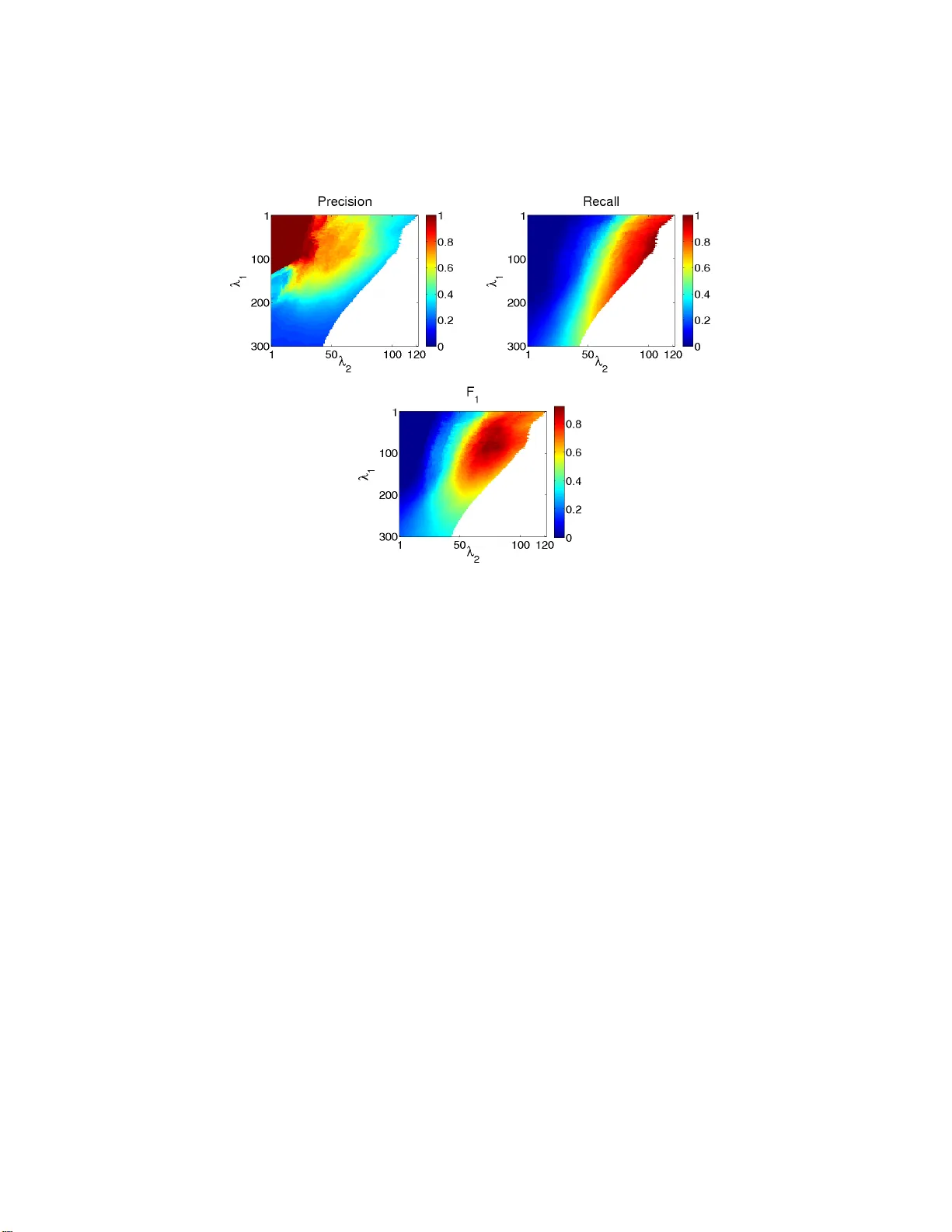
Estimating Net w orks With Jumps Mladen Kolar and Eric P . Xing Sc ho ol of Computer Science Carnegie Mellon Univ ersity Abstract W e study the problem of estimating a temp orally v arying coeﬃcient and v arying structure (VC VS) gra phical mo del underlying nonstatio nary time series data, such as social states of interacting individuals or microar- ra y expression proﬁles of gene netw orks, as opposed to i.i .d. data from an inv ariant model widely considered in cu rre nt literature of structural esti- mation. In particular, w e consider the scenario in whic h the mo del ev olves in a piece-wise constant fashion. W e prop ose a procedure that minimizes the so-called TESLA loss (i.e., temporally smoothed L1 regularized re- gression), which allo ws join tly estimating the partition b oundaries of th e VCVS mo del and th e co eﬃcie nt of th e sparse precision matrix on eac h block of the partition. A highly scala b le pro x i mal gradien t metho d is prop os ed to solv e the resultant con vex optimization problem; and the conditions for sparsistent estimation and the converg ence rate of b oth th e partition boun dari es and the net work structu re are established fo r the ﬁrst time for such estimato rs. 1 In tro duction Net works are a fundamental for m of r epresen ta tio n of relational infor mation underlying larg e, noisy data from v arious do m ains. F or exa mple, in a biolo g- ical study , no des of a net work can represent genes in one orga nism and edges can represent ass ociations or regulatory dependencies among genes. In a so- cial a nalysis, no des o f a netw ork can represe nt actor s and edges can represent int eractions o r friendships b et ween actor s. Exploring the statistical pro perties and hidden characteris t ics of netw ork ent ities, and the sto c hastic proces ses b e- hind tempo ral evolution of netw or k topolog ies is e ssen tial for computationa l knowledge discov er y a nd prediction based o n netw ork data. In man y dynamical en viro nmen ts, such as a dev eloping bio logical system, it is often technically imp ossible to experimentally determine the net work to p ologies sp eciﬁc to every time p oin t in a discr e t e time series. Resorting to computational inference metho ds, such as extant structura l le arning algor ithms, is also diﬃcult bec ause fo r every mo del unique to a single time p oin t, there exist as few as only a single sna p shot of the noda l states distributed accordingly to the mo de l in question. In this pa per, we consider a n estimation problem under a particular 1 dynamic context, where the mo del evolves piecewise co nstan tly , i.e., staying structurally in v ariant during unkno wn se gmen ts of time, and then jump to a diﬀerent structure. A p opular tec hnique f or deriving the net work s tr uctu re from iid s ample is to estimate a s parse precision matrix . The imp ortance of estimating pr ecision matrices with zeros w a s recognized by (Dempster, 19 7 2 ) who coined the term c ovarianc e sele ction . The elements of the precision matrix repres en t the as- so ciations or conditional cov ariances b et ween co rresponding v ar iables. Once a sparse precision matrix is estimated, a netw o r k can b e drawn by connecting v ariables whose corresp onding elements of the precision matrix are non-zero. Recent studies hav e sho wn that cov ariance selection methods bas ed o n the p e- nalized lik eliho o d maximizatio n can lead to a consisten t estimate of the net- work str uc tur e underlying a Gaus s ian Ma rk ov Random Fields (F an et a l., 2009; Ravikumar et al., 2008). Moreover, a particular pro cedure for co v a riance selec- tion known a s neigh b orho o d selection, which is built on ℓ 1 norm regular ized regres s ion, can pro duce a co n sistent estimate of the netw or k s t ructure when the sample is assumed to follow a general Marko v Random Field dis tr ibut ion whose structure cor responds to the netw ork in question (Ravikumar et al., 200 9 ; Meinshausen and B ¨ uhlmann, 2006; Peng et al., 2009). Speciﬁcally , a Mar k ov Random Field (MRF) is a pr obabilistic gra phica l model deﬁned o n a gra ph G = ( V , E ), where V = { 1 , . . . , p } is a vertex set co r responding to the set of random v aria bles to b e mo deled (in this pap er we call them no des and variables int erchangeably), and E ⊆ V × V is the edge set capturing conditional indecen- cies among these nodes. Let X = ( X 1 , . . . , X p ) ′ denote a p -dimensional random vector, who se elements are index e d by the nodes of the graph G . Under the MRF, a pa ir ( a, b ) is not an elemen t o f the edge set E if and only if the v ariable X a is conditionally indep enden t of X b given all the rest of v ar iables X V \{ a,b } , X a ⊥ X b | X V \{ a,b } . A distribution o ver X c a n b e deﬁned b y taking the fol- lowing log linear form that makes explicit use of the (presence and absence o f edges in the) edge set: p ( X ) ∝ exp { P ( a,b ) ∈ V θ ab X a X b } . When the elements of the random v ecto r X ar e discrete, e.g., X ∈ { 0 , 1 } p , the mo del is referr ed to as a discrete MRF, sometimes kno wn as an Ising model in sta t istics ph y sics communit y; wherea s when X is a con tinuous vector, the mo del is referred to as a Gauss ian graphica l model (GGM) becaus e one can e asily show that the p ( X ) abov e is actually a multiv aria te Gaussian. The MRF hav e b een widely used for modeling data with graphica l relational structures o ver a ﬁxed set of ent ities (W ain wrig h t a nd Jordan, 2008; Geto or and T ask ar, 2007). The vertices can describ e entities such a s genes in a biolo g ical re gulatory netw o rk, sto cks in the mar k et, or pe o ple in so ciet y; while the edges can describe relations hips betw een vertices, for exa mple, in ter action, corr elation o r inﬂuence. The statistical problem w e concern in this pap er is to estimate the struc - ture of the Gaussian graphical model fro m observed s a mples of no dal states in a dynamic w o rld. T raditional metho ds ha nd le this problem with the assump- tion that the samples ar e iid . Let D = { x 1 , . . . , x n } be an indep endent and identic al ly distribute d s ample according to a p -dimensional m ultiv ariate normal 2 distribution N p ( 0 , Σ ), where Σ is the co v ar iance matrix. Let Ω := Σ − 1 denote the precision ma t rix, with elemen ts ( ω ab ), 1 ≤ a, b ≤ p . Then one can obtain a n estimator of the Ω from D via optimizing a pro p er sta tis tica l loss function, such as likeliho od or penalized likelihoo d. As mentioned ea r lier, the precision matrix Ω enco des the conditional indep endence structure of the distribution and the pattern of the zero elemen ts in the precision matrix deﬁne the structure of the asso ciated gr aph G . There has been a dramatic growth of interest in recen t literature in the problem of co v ar iance selection, which deals with the graph estimation pro blem ab o ve. Existing w o rks ra nge fro m algorithmic developmen t fo cusing on eﬃcient estimation pro cedures, to theore tica l analysis focus ing on statistical guarantees of diﬀerent estimator s. W e do not intend to give an ex- tensive o verview of the literature here, but interested rea ders can follow the po in ters b ello w. In the cla s sical liter a ture (e.g. Lauritzen, 1996), pro cedures are develop ed for small dimensiona l graphs a nd commonly involv e hypothe- sis testing with greedy selectio n of edges. Mor e r ecen t literature estimates the sparse pr ecision matrix by o p timizing p enalized likelihoo d (Y uan and Lin, 2007; F an et al., 2 009; Banerjee e t al., 2 008 ; Rothman et al., 2008; F rie dma n et a l., 2008; Ravikumar et al., 2008; Guo et al., 2010b; Zhou et a l., 2008) or thr ough neighborho o d selection (Meinshausen and B¨ uhlmann, 2006; Peng et al., 2009; Guo et al., 20 10a ; W ang et al., 2009), where the structure of the graph is esti- mated by estimating the neigh bo rhoo d of ea ch no de. Both of these approaches are suitable fo r high-dimensional problems , ev en when p ≫ n , and can b e eﬃ- ciently implemen ted using scala ble con vex program s olv ers . Most of the ab o ve mentioned work ass umes that a s ingle inv ar ian t net work mo del is suﬃcien t to describe the dependencies in the obser ved data. How ever, when the observed da t a are no t iid , such an assumption is no t justiﬁable. F or example, when da t a consist of microarray measur emen ts of the gene expression levels collected throughout the cell cycle or development of a n organism, dif- ferent genes can be active during diﬀeren t stage s. This sugges t s that diﬀeren t distributions and hence diﬀerent netw or ks sho uld b e used to describ e the dep en- dencies b et ween measured v aria bles at diﬀ erent time in ter v als. In this paper, we are going to tackle the pr oblem of estimating the structur e of the GGM when the structure is allow ed to c hang e ov e r time. B y as s um ing that the pa- rameters o f the precision matrix c hang e with time, we obtain extra ﬂexibility to mo del a larger clas s of distributions while still retaining the in terpr etabilit y of the s t atic GGM. In par t icular, as the co eﬃcien ts of the precision matrix change ov er time, we also a llo w the structure of the underlying gra ph to c hang e as w ell. This se m i-parametr ic gener alization of the parametric mo del is referred to as a v arying co eﬃcient v arying structure (VCVS) model. Now, let { x i } i ∈ [ n ] ∈ R p be a sequence of n indep enden t observ ations (we use [ n ] to denote the set { 1 , . . . , n } ) from so m e p -dimens io nal m ultiv ariate normal distributions, not necess arily the same for every observ ation. L et {B j } j ∈ [ B ] be a disjoint pa rtitioning of the s e t [ n ] where each blo ck of the partition consists of consecutive elements, that is, B j ∩ B j ′ = ∅ for j 6 = j ′ and S j B j = [ n ] and B j = [ T j − 1 : T j ] := { T j − 1 , T j − 1 + 1 , . . . , T j − 1 } . Let T := { T 0 = 1 < T 1 < . . . < 3 T B = n + 1 } denote the set of partition b oundaries. W e consider the following mo del x i ∼ N p ( 0 , Σ j ) , i ∈ B j , (1) so that obser v ations indexed by elements in B j are p -dimensiona l rea lizations of a multiv ar ia te normal distribution with z ero mean and the cov ariance matrix Σ j = ( σ j ab ) a,b ∈ [ p ] . Let Ω j := ( Σ j ) − 1 denote the pr ecision matrix with ele m ents ( ω j ab ) a,b ∈ [ p ] . With the num b er o f pa rtitions, B , and the b oundaries of partitions, T , unkno wn, w e study the pro blem of estimating both the partition set { B j } and the non-zero ele m ents of the precision matrices { Ω j } j ∈ [ B ] from the sam- ple { x i } i ∈ [ n ] . No t e that in this w o rk we study a par ticular cas e of the VCVS mo del, where the coeﬃcients are piec e -wise constant functions of time. A sce- nario where the co eﬃcien ts are smo othly v a rying functions of time has b een considered in Zhou et al. (2008) fo r the GGM and in K olar et a l. (2010b) a nd Kolar and Xing (2009) for an Ising mo del. If the partitions {B j } j were known, the problem would b e trivially reduced to the setting ana lyzed in the previous work. Dealing w ith the unknown par tit ions, together with the s t ructure estimation of the model, ca lls for new methods. W e prop ose and a nalyze a metho d based on time-c ouple d n ei ghb orho o d sele ct i on , where the model estimates are forced to sta y similar across time using a fusion- t yp e tota l v ar iation p enalt y and the sparsity of each neighbor hoo d is o btained through the ℓ 1 pena lt y . Details of the appr oac h are given in § 2. The mo del in Eq. (1) is r elated to the v ar ying-coeﬃcie nt mo dels (e.g. Hastie a nd Tibshirani, 1 993 ) with the co eﬃcients being piece-wise constant func- tions. V arying co eﬃcient regre ssion mo dels with piece-wis e constant co eﬃcien ts are also known as segmented multiv aria te regressio n mo dels (Liu et al., 1997) or linear mo dels with structural changes (Ba i and P e r ron , 19 98 ). The structur a l changes are co mm only determined through hypo thesis testing and a separate linear mo del is ﬁt to eac h of the estimated segmen ts. In our work, we use the pena lized mo del selection approach to jointly estima te the partition b oundaries and the mo del par ameters. Little work ha s b een done so far tow a r ds mo deling dynamic net works and estimating changing precision matrices . Zho u et al. (2008) develops a nonpara - metric method for estimation of time-v arying GGM, where x t ∼ N p ( 0 , Σ ( t )) and Σ ( t ) is smoothly changing over time. The pro cedure is ba s ed on the penal- ized likelihoo d a pproac h of Y uan and Lin (20 07) with the empirical co v a riance matrix o btained using a kernel smo other. Our work is very diﬀerent from the one o f Zhou et a l. (2008), since under our a ssumptions the netw ork changes abruptly rather tha n smo othly . F urthermor e, as we outline in § 2, our estima- tion pro cedure is not based on the p enalized lik eliho o d appr oac h. Estimation of time-v ary ing Ising mo dels ha s b een discussed in Ahmed and Xing (2009) a nd Kolar et al. (2010 b ). Yin et al. (20 08 ) and K olar et al. (2010a) studied non- parametric w ays to estimate the conditional co v ar iance matrix. The w or k of Ahmed a nd Xing (20 09 ) is most simila r to our se tting, where they also use a fused-type pena lt y combined with an ℓ 1 pena lt y to estimate the structure of the verying Ising mo del. Here, in a ddit ion to fo cusing on GGMs, ther e is an 4 additional subtle, but important, diﬀerence to Ahmed and Xing (2009). In this work, we use a modiﬁca t ion of the fusion p enalt y (formally describ ed in § 2) which allows us to characterize the mo del selection co n sistency of o ur estimates and the conv ergence prop e rties of the estimated partition bo undaries, which is not av ailable in the earlier w o rk. The remaining of the pa per is org anized as follows. In § 2, we describ e our estimation pro cedure and pr o vide an eﬃcie nt ﬁr st-order optimization procedur e capable of estimating lar ge graphs. The o pt imization pro cedure is ba sed on the s m o othing pro cedure of Nesterov (200 5 ) and co n verges in O (1 / ǫ ) iterations, where ǫ is the desired a ccuracy . Our main theoretica l results are presented in § 3. In particular, w e show that the partition b oundaries are estimated consistently . F urthermore, the graph structure is consistently estimated on ev e ry blo c k of the partition that con tains enough samples. Numerical studies showing the ﬁnite sample perfor mance of our pr ocedure are given in § 4. The pro ofs of the main results are relega ted to § 6 , with some tec hnical details presen ted in Appendix . Notation Sch emes: F or clarity , w e end the intro duction with a summary of the notatio ns use d in the paper . W e use [ n ] to denote the set { 1 , . . . , n } and [ l : r ] to denote the set { l , l + 1 , . . . , r − 1 } . W e use B j to denote j -th block of the partition T . With s ome abuse of no tation, we also use B j to deno t e the s et [ T j − 1 : T j ]. The num b er of samples in the block B j is denoted a s |B j | . F or a set S ⊂ V , we use the notatio n X S to denote the set { X a : a ∈ S } of random v ar iables. W e use X to denote the n × p matrix whose rows consist of observ ations. The vector X a = ( x 1 ,a , . . . , x n,a ) ′ denotes a column o f matrix X and, s imilarly , X S = ( X b : b ∈ S ) denotes the n × | S | sub-matrix of X whose columns are indexed by the s et S and X B j denotes the sub-matrix |B j | × p w ho se rows are indexed by the set B j . F or simplicit y of nota t ion, we will use \ a to denote the index set [ p ] \{ a } , X \ a = ( X b : b ∈ [ p ] \{ a } ). F or a v ecto r a ∈ R p , we let S ( a ) deno te the set o f non-zero comp onen ts of a . Throughout the pap er, we use c 1 , c 2 , . . . to denote p ositiv e constants whose v alue ma y change from line to line. F o r a vector a ∈ R n , deﬁne || a || 1 = P i ∈ [ n ] | a i | , || a || 2 = q P i ∈ [ n ] a 2 i and || a || ∞ = max i | a i | . F or a symmetr ic matrix A , Λ min ( A ) denotes the smalle s t and Λ max ( A ) the lar gest eigenv alue. F or a m atrix A (not nece ssarily s ymmetric), we use | | | A | | | ∞ = max i P j | A ij | . F or tw o v ectors a , b ∈ R n , the dot pro duct is denoted h a , b i = P i ∈ [ n ] a i b i . F or t wo matrices A , B ∈ R n × m , the dot pro duct is denoted as h h A , B i i = tr( A ′ B ). Giv en tw o sequences { a n } and { b n } , the notation a n = O ( b n ) means that there exists a c o nstan t c 1 such that a n ≤ c 1 b n ; the no tation a n = Ω( b n ) means that there exists a constant c 2 such that a n ≥ c 2 b n and the notation a n ≍ b n means that a n = O ( b n ) and b n = O ( a n ). Similarly , we will use the notation a n = o p ( b n ) to denote that b − 1 n a n conv erg es to 0 in probability . 5 T able 1: Summary of symbo ls used thro ughout the paper Symbol Meaning Example [ n ] used to denote the s et { 1 , . . . , n } [ t 1 : t 2 ] used to denote the set { t 1 , t 1 + 1 , . . . , t 2 − 1 } i used for indexing related to samples x i or β a · ,i j, k used for indexing related to block θ a,j or S k a a, b used for indexing no des in a gr aph a, b ∈ V G the graph co nsisting of v er tice s and edges G = ( V , E ) V t he set o f no des in a gr aph V = [ p ] E i the set of edges at time i X a the component of a random vector X indexed b y the vertex a β a · ,i the v ecto r of regr ession co eﬃcien ts for sa mple i θ a,j the vector of regr ession co eﬃcien ts for blo c k j T the set of partition boundar ies { τ j } j the set o f boundar y fractions T j = ⌊ nτ j ⌋ B j an index set for the sa mples in the partition j B j ⊂ [ n ] B denotes the num b er of partitions S j a the set o f neigh bo rs of node a in blo c k j S ( θ a,j ) the set of non-zero elemen ts of θ a,j ¯ S j a the closure of S j a ¯ S j a = S j a ∪ { a } N j a no des not in the neighbor hoo d of the no de a in block j N j a = [ p ] \ ¯ S j a \ a the set o f all v er tice s excluding the vertex a \ a = [ p ] \{ a } | · | cardinality of a set or absolute v alue Σ the cov ariance matr ix σ ab an ele m ent of the co v ar iance ma trix Ω the precision matrix ω ab an elemen t of the precision matrix h· , ·i the dot pr o duct h a , b i = a ′ b h h· , ·i i the dot pro duct b et ween matr ices h h A , B i i = tr ( A ′ B ) ξ min the minim um change b et ween regre ssion co e ﬃ cient || θ a,j − θ a,j − 1 || 2 ≥ ξ min θ min the minim um size of a co eﬃcien t | θ a,j b | ≥ θ min ∆ min the minim um size of a blo c k |B j | ≥ ∆ min 6 2 Graph estimation via T e mp oral-Diﬀerence Lasso In this section, we introduce o ur time-v ar ying co v ar iance s election pro cedure, which is based o n the time-coupled neigh b orho od s election using the fused-t yp e pena lt y . W e ca ll the pr oposed pro cedure T emp oral-Diﬀerence Lasso ( TD-L asso ). W e sta r t by reviewing t he basic neigh b orho od selection pr o cedure, whic h has previously b e en used to estimate g raphs in, for exa mple, Peng et al. (2009), Meinshausen and B ¨ uhlmann (2 006 ), Ravikumar et al. (20 09 ) and Guo et al. (2010 a ). W e star t by r elating the elements of the precision matrix Ω to a reg r ession problem. Let the set S a to denote the neighborho od of the no de a . Denote ¯ S a the clo sure of S a , ¯ S a := S a ∪{ a } , a nd N a the s e t o f no des not in the neig h b orhoo d of the node a , N a = [ p ] \ ¯ S a . It holds that X a ⊥ X N a | X S a . The neigh b orho od of the no de a can b e e asily seen from the non-zer o pattern of the elemen ts in the precision matrix Ω , S a = { b ∈ [ p ] \ { a } : ω ab 6 = 0 } . See Lauritzen (1996) for more details. It is a w ell kno wn r esult for Gaus s ian g raphical models that the elements of θ a = argmin θ ∈ R p − 1 E ( X a − X b ∈\ a X b θ b ) 2 are giv e n b y θ a b = − ω ab /ω aa . Therefore, the neigh b orho od of a no de a , S a , is equal to the set of non-zero co eﬃcien ts of θ a . Using the expression for θ a , we can w r ite X a = P b ∈ S a X b θ a b + ǫ , where ǫ is indepe nd ent of X \ a . The neighborho od selection pro cedure w as motiv ated by the a bov e relation- ship b et ween the r egression co eﬃcien ts and the elements of the precision ma t rix. Meinshausen and B ¨ uhlmann (2 006) prop osed to solve the following optimization pro cedure ˆ θ a = ar gmin θ ∈ R p − 1 1 n || X a − X \ a θ || 2 2 + λ || θ || 1 (2) and prov ed that for iid sa m ple the non-zero coe ﬃcie n ts of ˆ θ a consistently esti- mate the neighborho od of the no de a , under a suitably chosen p enalt y parameter λ . In this pap er, w e build on the neighbourho o d selection procedure to esti- mate the changing g raph str u cture in mo del (1). W e use S j a to deno t e the neighborho o d of th e no de a on the block B j and N j a to denote no des not in the neighborho od of the node a on the j -th blo c k, N j a = V \ S j a . Co nsider the following estimation pro cedure ˆ β a = argmin β ∈ R p − 1 × n L ( β ) + p en λ 1 ,λ 2 ( β ) (3) where the loss is deﬁned for β = ( β b,i ) b ∈ [ p − 1] ,i ∈ [ n ] as L ( β ) := X i ∈ [ n ]  x i,a − X b ∈\ a x i,b β b,i  2 (4) 7 and the p enalty is deﬁned as pen λ 1 ,λ 2 ( β ) := 2 λ 1 n X i =2 || β · ,i − β · ,i − 1 || 2 + 2 λ 2 n X i =1 X b ∈\ a | β b,i | . (5) The pena lt y term is constructed from tw o terms. The ﬁrst term ensures that the solution is going to be piece wise constant fo r some par tition of [ n ] (possibly a t rivial one). The ﬁrst term can be seen a s a s parsity inducing term in the tempo ral domain, since it penalizes the diﬀerence b etw e e n the co eﬃcients β · ,i and β · ,i +1 at suc c essive time-po int s. The second term results in estimates that hav e man y zero coe ﬃcie nts within ea ch block o f the partition. The estimated set o f partition b oundar ies ˆ T = { ˆ T 0 = 1 } ∪ { ˆ T j ∈ [2 : n ] : ˆ β a · , ˆ T j 6 = ˆ β a · , ˆ T j − 1 } ∪ { ˆ T ˆ B = n + 1 } contains indices of po ints a t which a change is estimated, with ˆ B being an estimate of the num b er of blocks B . The estimated num b er of the blo ck ˆ B is controlled through the user deﬁned penalty para meter λ 1 , while the sparsity of the neigh b o rho o d is controlled throug h the p enalty parameter λ 2 . Based on the es timated set of partition b oundar ies ˆ T , w e can deﬁne the neighborho o d estimate of the no de a for each estimated blo ck. Let ˆ θ a,j = ˆ β a · ,i , ∀ i ∈ [ ˆ T j − 1 : ˆ T j ] b e the estimated co eﬃcient vector for the blo ck ˆ B j = [ ˆ T j − 1 : ˆ T j ]. Using the estimated vector ˆ θ a,j , we deﬁne the neighbor ho o d estimate of the no de a for the block ˆ B j as ˆ S j a := S ( ˆ θ a,j ) := { b ∈ \ a : ˆ θ a,j b 6 = 0 } . Solving (3) for each no de a ∈ V gives us a ne ig hborho o d es timate for eac h no de. Combining the neighborho o d e stimates we can obtain an estimate of the graph structure for each p oint i ∈ [ n ]. The c hoice of the penalty term is motiv ated by the work on penalizatio n using total v aria tio n (Rinaldo, 2 009; Mammen and v an de Geer, 19 97), which results in a piece-wis e constant approximation of an unkno wn regressio n func- tion. The fusio n- p e nalty has als o b een applied in th e co ntext of multiv a r iate linear r egress ion Tibshirani et al. (2005), where the co eﬃcients that a re s patially close, ar e also bia sed to ha ve simila r v alues. As a result, near by coeﬃcie nts are fused to the s a me e s timated v alue. Instead of p enalizing the ℓ 1 norm on the diﬀerence b etw ee n co eﬃcients, we use the ℓ 2 norm in order to enforce that all the c hang es o ccur at the same po int. The ob jective (3) estimates the neigh b or ho o d of one no de in a graph for all time-po ints. After solving the ob jective (3 ) for all no des a ∈ V , w e need to combine them to obtain the gr aph str ucture. W e will use the following pro cedure to co mbine { ˆ β a } a ∈ V , ˆ E i = { ( a, b ) : max( | β a b,i | , | β b a,i | ) > 0 } , i ∈ [ n ] . That is, an edge b etw e e n no des a and b is included in the gra ph if at lea st one of the no des a or b is included in the neighborho o d of the other no de. W e 8 use the max op er ator to combine diﬀeren t neig hborho o ds as we believe that for the purpo se of net work explor a tion it is more imp or tant to occ asionally include spurious edges than to omit relev ant o nes. F or further discuss ion on the diﬀerences b etw een the min and t he ma x com bina tio n, we refer an in terested reader to Banerjee et al. (200 8). 2.1 Numerical pro c edure Finding a minimizer ˆ β a of (3) can b e a computatio nally c ha llenging task for a n oﬀ-the-shelf conv ex optimization pro cedur e. W e prop o se too use an acc elerated gradient metho d with a smo othing technique (Nesterov, 200 5), whic h conv erg es in O (1 /ǫ ) iterations where ǫ is the de s ired accuracy . W e s tart by deﬁning a smo oth approximation of the fused p enalty term. Let H ∈ R n × n − 1 be a matrix with elements H ij =    − 1 if i = j 1 if i = j + 1 0 otherwise. With the matrix H we can r e w r ite the fused p enalty term a s 2 λ 1 P n − 1 i =1 || ( β H ) · ,i || 2 and using the fa c t that the ℓ 2 norm is self dual (for example, see Boyd and V andenber ghe, 2004) w e hav e the following repr e sentation 2 λ 1 n X i =2 || β · ,i − β · ,i − 1 || 2 = max U ∈Q h h U , 2 λ 1 β H i i (6) where Q := { U ∈ R p − 1 × n − 1 : || U · ,i || 2 ≤ 1 , ∀ i ∈ [ n − 1] } . The follo wing function is deﬁned as a smo oth approximation to the fused p enalty , Ψ µ ( β ) := max U ∈Q h h U , 2 λ 1 β H i i − µ || U || 2 F (7) where µ > 0 is the smo othness parameter . It is easy to see that Ψ µ ( β ) ≤ Ψ 0 ( β ) ≤ Ψ µ ( β ) + µ ( n − 1) . Setting the smo othness parameter to µ = ǫ 2( n − 1) , the correct rate of conv er g ence is ens ur ed. L e t U µ ( β ) be the optimal solution o f the max imiza tion problem in (7), whic h can b e obtained analytica lly as U µ ( β ) = Π Q  λ β H µ  (8) where Π Q ( · ) is the pro jection op erator onto the set Q . F rom Theor e m 1 in Nesterov (2005), we hav e that Ψ µ ( β ) is contin uously diﬀere ntiable a nd conv ex , with the gr adient ∇ Ψ µ ( β ) = 2 λ 1 U µ ( β ) H ′ (9) that is Lipschitz co ntin uous. 9 With the ab ove deﬁned smo o th approximation, w e fo cus on minimizing the following ob jective min β ∈ R p − 1 × n F ( β ) := min β ∈ R p − 1 × n L ( β ) + Ψ µ ( β ) + 2 λ 2 || β || 1 . F ollowing Beck and T eboulle (2009) (see also Nesterov (2007)), we deﬁne the following quadratic approximation of F ( β ) at a p oint β 0 Q L ( β , β 0 ) := L ( β 0 ) + Ψ µ ( β 0 ) + h h β − β 0 , ∇L ( β 0 ) + ∇ Ψ( β 0 ) i i + L 2 || β − β 0 || 2 F + 2 λ 2 || β || 1 (10) where L > 0 is the par ameter chosen as an upp er bounds for the Lipschitz constant of ∇L + ∇ Ψ. Let p L ( β 0 ) be a minimizer o f Q L ( β , β 0 ). Ignoring constant terms, p L ( β 0 ) can b e obtained as p L ( β 0 ) = argmin β ∈ R p − 1 × n 1 2     β −  β 0 − 1 L  ∇L + ∇ Ψ  ( β 0 )      2 F + 2 λ 2 L   β   1 . It is clear tha t p L ( β 0 ) is the unique minimizer, whic h can b e obtained in a clos ed form, a s a result of the soft-thr e sholding, p L ( β 0 ) = T  β 0 − 1 L  ∇L + ∇ Ψ  ( β 0 ) , 2 λ 2 L  (11) where T ( x, λ ) = s ig n( x ) max(0 , | x | − λ ) is the soft-thresholding op er ator that is applied ele ment -wise. In prac tice , an upp er bound o n the Lipschitz constan t of ∇L + ∇ Ψ can b e exp ensive to compute, so the parameter L is g oing to be determined iteratively . Combining all of the ab ov e, we ha ve the follo wing algor ithm. In the algo - rithm, γ is a consta nt used to incr ease the estimate of the Lipsc hitz co ns tant L . Compared to the gradient descent metho d (whic h can be obtain b y iterating β k +1 = p L ( β k )), the acceler ated gradient metho d up dates tw o sequences { β k } and { z k } recur sively . Instead o f p erforming the gradient step from the latest approximate so lutio n β k , the gr a dient step is perfor med fr om the search point z k that is obtained as a linear combination of the last to approximate solutions β k − 1 and β k . Since the co ndition F ( p L ( z k )) ≤ Q L ( p L ( z k ) , z k ) is satisﬁed in every iteration, we ha ve the algorithm conv er ges in O (1 / ǫ ) iterations following Beck and T eboulle (2009). As the con vergence cr iterion, we stop iterating once the relative c hang e in the ob jective v alue is below so me thre s hold v a lue. 2.2 T u ning parameter select ion The pena lty par ameters λ 1 and λ 2 control the complexity of the estimated mo del. In this w o rk, we prop ose to us e the BIC sc o re to select the tuning parameters . Deﬁne the BIC sco re for ea ch no de a ∈ V as BIC a ( λ 1 , λ 2 ) := log L ( ˆ β a ) n + log n n X j ∈ [ ˆ B ] | S ( ˆ θ a,j ) | (12) 10 Algorithm: Accelerated Gr adient Metho d for Eq ua tion (3) Input : X ∈ R n × p , β 0 ∈ R p − 1 × n , γ > 1, L > 0, µ = ǫ 2( n − 1) Output : ˆ β a Initialize k := 1, α k := 1, z k := β 0 rep eat while F ( p L ( z k )) > Q L ( p L ( z k ) , z k ) do L := γ L β k := p L ( z k ) (using E q. (11)) α k +1 := 1+ √ 1+4 α k 2 z k +1 := β k + α k − 1 α k +1  β k − β k − 1  un til c onver genc e ˆ β a := β k where L ( · ) is deﬁned in (4) and ˆ β a = ˆ β a ( λ 1 , λ 2 ) is a solution of (3). The p e na lty parameters can now b e chosen as { ˆ λ 1 , ˆ λ 2 } = argmin λ 1 ,λ 2 X a ∈ V BIC a ( λ 1 , λ 2 ) . (13) W e will use the ab ov e formula to select the tuning parameter s in our simulations, where w e are going to search for the b est choice of parameters over a g rid. 3 Theoretical result s This section is go ing to a ddress the statistical pro p erties o f the estimation pro- cedure presented in Section 2. The pro p erties are a ddressed in an asy mptotic framework by letting the sample size n grow, while keeping the other par ameters ﬁxed. F or the asymptotic framework to make sense, w e assume tha t there exists a ﬁxed unknown sequence of n umbers { τ j } that deﬁnes the partition b oundarie s as T j = ⌊ nτ j ⌋ , where ⌊ a ⌋ denotes the largest integer smaller that a . This assures that as the num b er of s amples gr ow, the sa me fra ction of samples falls into every partition. W e call { τ j } the b oundary fractions. W e g ive suﬃcient conditions under which the sequenc e { τ j } is consistently estimated. In particular, if the num b er of partition blo cks is estimated corr ectly , then we show that max j ∈ [ B ] | ˆ T j − T j | ≤ nδ n with pr obability tending to 1 , wher e { δ n } n is a no n-increas ing sequence of positive n um ber s that tends to zero. If the n umber of par tition segmen ts is over estimated, then w e s how t hat for a distance deﬁned for t wo sets A and B as h ( A, B ) := sup b ∈ B inf a ∈ A | a − b | , (14) 11 we hav e h ( ˆ T , T ) ≤ nδ n with pro ba bility tending to 1. With the bo undary segments consistently estimated, we further show that under suitable conditions for each no de a ∈ V the cor rect neigh bo rho o d is selected on all estimated blo ck partitions that a re suﬃciently large. The pro of tec hnique employed in this section is quite involv ed, so w e brieﬂy describ e the steps used. Our analysis is based on careful insp ection of the op- timalit y conditions that a solution ˆ β a of the optimizatio n problem (3) need to satisfy . The optimality conditions for ˆ β a to b e a solution of (3) are g iven in § 3.2. Using the o ptimality conditions , w e esta blis h the ra te of conv e r gence for the par - tition b oundar ies. T his is done b y pro of by contradiction. Supp ose that there is a solution with the partition boundar y ˆ T that satisﬁes h ( ˆ T , T ) ≥ nδ n . Then we show that, with high-probability , all suc h solutio ns will not satisfy the K KT conditions and therefore cannot be o ptimal. This shows that all the solutions to the optimization problem (3) result in partition boundar ie s tha t a re “close” to the true partition boundaries , with high-probability . Once it is established that ˆ T and T satisfy h ( ˆ T , T ) ≤ nδ n , we can further show tha t the neigh b or ho o d estimates are consis tent ly estimated, under the as sumption that the estimated blo cks of the par tition hav e enough samples. This part of the analysis fol- lows the commonly used strategy to prov e that the Lass o is spar s istent (see for example Bunea, 2008; W ainwrigh t, 2009; Meinshausen and B ¨ uhlmann, 200 6), how ever imp ortant modiﬁca tions are required due to the fact that p osition of the partition b oundar ies are b eing estimated. Our analysis is going to fo cus on one no de a ∈ V and its neighbor ho o d. How ever, using the union bound over all no des in V , we will b e able to carry ov er conclusions to the whole gr aph. T o simplify o ur notation, when it is clea r from the c o ntext, we will o mit the superscr ipt a and write ˆ β , ˆ θ and S , e tc., to denote ˆ β a , ˆ θ a and S a , etc. 3.1 Assumptions Before pr esenting our theoretical res ults, we give so me deﬁnitions and assump- tions that are g oing to be used in this section. Let ∆ min := min j ∈ [ B ] | T j − T j − 1 | denote the minimum le ng th b etw een change p o int s, ξ min := min a ∈ V min j ∈ [ B − 1] || θ a,j +1 − θ a,j || 2 denote the minimum jump size a nd θ min = min a ∈ V min j ∈ [ B ] min b ∈ S j | θ a,j b | the minim um coe ﬃcie nt size. Througho ut the section, we as sume that the fol- lowing holds. A1 There ex ist t wo co nstants φ min > 0 and φ max < ∞ such that φ min = min { Λ min ( Σ j ) : j ∈ [ B ] , a ∈ V } and φ max = max { Λ max ( Σ j ) : j ∈ [ B ] , a ∈ V } . A2 V ariables are scale d so that σ j aa = 1 for all j ∈ [ B ] and all a ∈ V . 12 The a s sumption A1 is commonly us ed to ensure that the mo del is iden tiﬁable . If the p o pula tion cov ar iance matrix is ill-c o nditioned, the ques tio n of the co r rect mo del iden tiﬁcation if not well deﬁned, as a neighbor ho o d of a node may not be uniquely deﬁned. The ass umption A2 is assumed for the simplicit y o f the presentation. T he common v ariance can b e obtained through s caling. A3 There ex ists a co nstant M > 0 suc h that max a ∈ V max j,k ∈ [ B ] k θ a,k − θ a,j k 2 ≤ M . The assumption A3 states that the diﬀerence b etw ee n co eﬃcients on tw o dif- ferent blocks, || θ a,k − θ a,j || 2 , is b ounded for all j, k ∈ [ B ]. This assumption is simply s a tisﬁed if the co eﬃcients θ a were b ounded in the ℓ 2 norm. A4 There ex ist a cons tant α ∈ (0 , 1], suc h that the following holds max j ∈ [ B ] | | | Σ N j a S j a ( Σ S j a S j a ) − 1 | | | ∞ ≤ 1 − α, ∀ a ∈ V . The ass umption A4 states that the v ar iables in the neig hborho o d of the node a , S j a , are not too corr elated with the v ariables in the set N j a . This assump- tion is necessar y and s uﬃcient for corr ect iden tiﬁcation of the relev ant v ari- ables in the Lasso reg ression problems (see for ex ample Zhao and Y u, 2 006; v an de Geer and B¨ uhlmann, 2009). Note that this condition is suﬃcient a lso in our case when the correct partition bo undaries are not known. A5 The minim um co eﬃcient size θ min satisﬁes θ min = Ω( p log( n ) /n ). The low er b o und on the minim um coe ﬃcie nt size θ min is necessa ry , since if a partial corr elation coeﬃcient is to o clos e to zero the edge in the gra ph w ould not b e detectable. A6 The s e quence o f partition bounda r ies { T j } sa tisfy T j = ⌊ n τ j ⌋ , where { τ j } is a ﬁxed, unknown seq uence of the bounda ry fractions b elo nging to [0 , 1 ]. The a ssumption is needed for the asymptotic setting. As n → ∞ , there will be enoug h sample points in each of the blo cks to estimate the neigh b o rho o d o f no des correctly . 3.2 Con vergence of the partition b oundaries In this subsection we establish the rate of conv erg ence of the bo undary partitions for the es timator (3). W e start by g iving a lemma that c haracter izes solutions of the optimization pr oblem given in (3). Note that the o ptimization problem in (3) is conv ex, howev er, ther e may b e multiple solutions to it, since it is no t strictly con vex. 13 Lemma 1. A matrix ˆ β is op timal for the optimization pr oblem (3) if and only if ther e exist a c ol le ction of su b gr adient ve ctors { ˆ z i } i ∈ [2: n ] and { ˆ y i } i ∈ [ n ] , with ˆ z i ∈ ∂ || ˆ β · ,i − ˆ β · ,i − 1 || 2 and ˆ y i ∈ ∂ || ˆ β · ,i || 1 , that satisﬁes n X i = k x i, \ a h x i, \ a , ˆ β · ,i − β · ,i i − n X i = k x i, \ a ǫ i + λ 1 ˆ z k + λ 2 n X i = k ˆ y i = 0 (15) for al l k ∈ [ n ] and ˆ z 1 = ˆ z n +1 = 0 . The following theor em provides the conv ergence ra te of the estimated b ound- aries o f ˆ T , under the ass umption that the co r rect num b er of blocks is known. Theorem 2. L et { x i } i ∈ [ n ] b e a se quenc e of obse rvation ac c or ding to the mo del in (1) . Assume that A1 - A3 and A5 - A6 hold. Supp ose that the p enalty p ar ameters λ 1 and λ 2 satisfy λ 1 ≍ λ 2 = O ( p log( n ) /n ) . (16) L et { ˆ β · ,i } i ∈ [ n ] b e any solution of (3) and let ˆ T b e the asso ciate d estimate of the blo ck p artition. L et { δ n } n ≥ 1 b e a non-incr e asing p ositive se quenc e that c onver ges to zer o as n → ∞ and satisﬁes ∆ min ≥ nδ n for al l n ≥ 1 . F urt hermor e, supp ose that ( nδ n ξ min ) − 1 λ 1 → 0 , ξ − 1 min √ pλ 2 → 0 and ( ξ min √ nδ n ) − 1 √ p lo g n → 0 , then if | ˆ T | = B + 1 the fol lowing hol ds P [ ma x j ∈ [ B ] | T j − ˆ T j | ≤ nδ n ] n →∞ − − − − → 1 . Suppo se that δ n = (log n ) γ /n for some γ > 1 a nd ξ min = Ω( p log n/ (log n ) γ ), the conditions of theor em 5 ar e s atisﬁed, and we hav e that the sequence o f bo undary fractions { τ j } is consisten tly estimated. Since the b oundar y fractions are cons is tent ly estimated, we will see below that the estimated neig hborho o d S ( ˆ θ j ) on the blo ck ˆ B j consistently recovers the true neigh bo rho o d S j . Unfortunately , the co rrect b o und on the num b er of blo ck B may not b e known. How ever, a conserv ative upper bound B max on the n umber of blo cks B ma y be kno wn. Suppose that the sequence o f o bs erv ation is o ver seg mented, with the num b er of estimated blo cks bounded by B max . Then the following prop osition giv e s a n upp er b ound on h ( ˆ T , T ) where h ( · , · ) is deﬁned in (14). Prop ositi on 3. L et { x i } i ∈ [ n ] b e a se quenc e of observation ac c or ding to the mo del in (1) . Assu m e that the c onditions of t he or em 2 ar e satisﬁe d. L et ˆ β b e a solution of (3 ) and ˆ T t he c orr esp onding set of p artition b oundaries, with ˆ B blo cks. If the numb er of blo cks satisfy B ≤ ˆ B ≤ B max , then P [ h ( ˆ T , T ) ≤ nδ n ] n →∞ − − − − → 1 . The pro of of the prop o sition follows the sa me ideas of theorem 2 and its sketc h is given in the appendix. The above prop os ition as sures us that even if the n umber of blo cks is overesti- mated, there will b e a partition boundary close to ev er y true unknown par tition bo undary . 14 Figure 1: The ﬁgure illustrates where we exp ect to estimate a neighbo rho o d of a no de consistently . The blue r e gion corresp onds to the o verlap b etw een the true blo ck (bo unded by gray lines) and the es timated blo ck (bo unded by black lines). If the blue region is m uch larger tha n the orange regio ns, the additional bias int ro duced from the sa mples from the orange region will not considera bly aﬀect the estimation of the neighbor ho o d of a no de on the blue reg ion. How ever, w e cannot hop e to consistently estimate the neighbor ho o d of a no de on the o range region. 3.3 Correct neigh b o r ho o d selection In this section, we give a result on the consistency of the neighborho o d es ti- mation. W e will sho w that whenever the estimated blo ck ˆ B j is large enoug h, say | ˆ B j | ≥ r n where { r n } n ≥ 1 is an incr easing sequence of n umbers that s atisfy ( r n λ 2 ) − 1 λ 1 → 0 and r n λ 2 2 → ∞ as n → ∞ , we ha ve that S ( ˆ θ j ) = S ( β k ), where β k is the true parameter o n the true block B k that ov erlaps ˆ B j the most. Figure 1 illus trates this idea . The blue region in the ﬁgure denotes the o verlap betw een the true block and the estimated block of the pa r tition. The or ange region corres p o nds to the overlap of the estima ted blo ck with a diﬀerent true blo ck. If the blue regio n is considera bly larger than the orange region, the bias coming from the sample from the orange region will not be s tr ong eno ugh to disable us from s electing the correct neig hborho o d. On the other hand, since the orange reg ion is small, as seen from Theorem 2, there is little hop e of es timating the neigh b o rho o d co rrectly on that po rtion of the sample. Suppo se that we kno w that there is a solution to the optimization pr ob- lem (3) with the partition bounda ry ˆ T . Then that solution is als o a minimizer of the following ob jective min θ 1 ,..., θ ˆ B X j ∈ ˆ B || X ˆ B j a − X ˆ B j \ a θ j || 2 2 + 2 λ 1 ˆ B X j =2 || θ j − θ j − 1 || 2 + 2 λ 2 ˆ B X j =1 | ˆ B j ||| θ j || 1 . (17) Note that the problem ( 17) does not give a practical w ay of solving (3), but will help us to re a son ab out the s olutions of (3). In particular , while there may b e m ultiple solutions to the problem (3), under some co nditions, w e can characterize the sparsity pattern of any solutio n that ha s s pe ciﬁed partition bo undaries ˆ T . Lemma 4 . L et ˆ β b e a solution to (3) , with ˆ T b eing an asso ciate d estimate of the p artition b oundaries. Supp ose that the su b gr adient ve ctors s atisfy | ˆ y i,b | < 1 15 for al l b 6∈ S ( ˆ β · ,i ) , then any other solut ion ˜ β with the p artition b oun daries ˆ T satisfy ˜ β b,i = 0 fo r al l b 6∈ S ( ˆ β · ,i ) . The ab ov e Lemma states suﬃcient co nditions under which the sparsity pa t- ter of a solution with the partition bo undary ˆ T is unique. Note, how e ver, that there may other solutio ns to (3) that hav e diﬀeren t partition bounda r ies. Now, we a re ready to state the following theor em, whic h establishes that the correct neighborho o d is selected o n every suﬃcient ly larg e estimated blo ck of the partition. Theorem 5. L et { x i } i ∈ [ n ] b e a se quenc e of observation ac c or ding to the mo del in (1) . Assume that t he c onditions of the or em 2 ar e satisﬁe d. In addition, supp ose that A4 also holds. Then, if | ˆ T | = B + 1 , it holds that P [ S k = S ( ˆ θ k )] n →∞ − − − − → 1 , ∀ k ∈ [ B ] . Under the as s umptions of theorem 2 each estimated block is of siz e O ( n ). As a result, there are e no ugh samples in eac h block to consisten tly e stimate the underlying neighbor ho o d structure. Obs e r ve that the neigh b o rho o d is consis- ten tly estimated at each i ∈ ˆ B j ∩ B j for all j ∈ [ B ] and the error is made only on the small fraction of sa mples, when i 6∈ ˆ B j ∩ B j , whic h is of order O ( nδ n ). Using prop o sition 3 in place of theorem 2, it can be similarly shown that, for a large fraction of samples, the neigh bo rho o d is consistently estimated even in the case of over-segmentation. In pa rticular, whenever there is a suﬃciently large es timated block, with | ˆ B k ∩ B j | = O ( r n ), it holds that S ( ˆ B k ) = S j with probability tending to o ne. 4 Numerical studies In this section, we present a small numerical study on the prop ose d a lgorithm on sim ulated netw ork s . A full p erfor mance tes t and application o n real world data is b e yond the scope of this pap er which mainly focuses o n the theory of time-v arying mo del e s timation. In all of our simulations studies we set p = 3 0 and B = 3 with |B 1 | = 80 , |B 2 | = 130 and |B 3 | = 90, s o that in to tal we hav e n = 30 0 samples. W e consider t wo t yp es of random netw o rks: a chain and a nearest neighbor net work. W e measure the p e rformance o f the estimation pro cedure o utlined in § 2 o n the following metrics: av erage precision o f estimated edges, av er age recall of estimated edges and a verage F 1 score which combines the pr ecision and reca ll scor e. The precision, r ecall and F 1 score are resp ectively 16 Figure 2: A chain gr aph deﬁned as pre cision = 1 n X i ∈ [ n ] P a ∈ [ p ] P p b = a +1 1 I { ( a, b ) ∈ ˆ E i ∧ ( a, b ) ∈ E i } P a ∈ [ p ] P p b = a +1 1 I { ( a, b ) ∈ ˆ E i } rec a l l = 1 n X i ∈ [ n ] P a ∈ [ p ] P p b = a +1 1 I { ( a, b ) ∈ ˆ E i ∧ ( a, b ) ∈ E i } P a ∈ [ p ] P p b = a +1 1 I { ( a, b ) ∈ E i } F 1 = 2 ∗ pre cision ∗ r ecal l pre cision + r ecal l . Our results are av eraged o ver 50 simulation runs. W e compare our algor ithm against an o racle algo rithm which exactly knows the true pa rtition b oundar ies. In this case, it is only needed to run the algo r ithm of Meinshausen a nd B ¨ uhlmann (2006) o n ea ch blo ck of the pa rtition independently . W e use a BIC criterion to select the tuning parameter for this or acle pr o cedure as des c rib ed in Peng et al. (2009). Chain netw orks. W e follow the sim ulation in F an et al. (20 09) to generate a chain net work (se e Figur e 2 ). This netw or k corr esp onds to a tridia gonal precision matrix (a fter an appr opriate permutation of no des). The netw ork is generated a s follows. First, we choo se gener ate a random p er mu tation π of [ n ]. Next, the cov ariance matrix is ge ne r ated as follows: the element at pos itio n ( a, b ) is chosen as σ ab = exp( −| t π ( a ) − t π ( b ) | / 2) where t 1 < t 2 < . . . < t p and t i − t i − 1 ∼ Unif (0 . 5 , 1 ) for i = 2 , . . . , p . This pro ces ses is re p ea ted three times to obtain three diﬀer ent cov aria nce ma tr ices, from which we sample 80, 1 3 0 and 90 sa mples r esp ectively . F or illustrativ e purpo ses, Figure 3 plots th e precision, recall and F 1 score computed for diﬀerent v alues of the p enalty parameters λ 1 and λ 2 . T able 2 shows the precisio n, r ecall and F 1 score for the parameters chosen us ing the BIC sco re describ ed in 2.2. The num ber s in parentheses c orresp o nd to standa rd deviation. Due to the fact that there is some erro r in estimating the parti- tion b oundar ies, we observe a decrease in p erfo rmance compa red to the oracle pro cedure that knows the corr ect p osition of the par tition b ounda ries. Nearest ne igh b ors ne t works. W e genera te nearest neighbor netw orks following the pro cedure outlined in Li and Gui (2006). F or each no de, w e dra w T able 2: P er formance on chain netw ork s Metho d name Precisio n Recall F 1 score TD-Lasso 0.84 (0 .04) 0.80 (0 .04) 0.82 (0 .04) Oracle proce dur e 0.97 (0 .02) 0.89 (0 .02) 0.93 (0 .02) 17 Figure 3: Plots of the precision, recall and F 1 scores as functions of the p enalty parameters λ 1 and λ 2 for chain netw orks . The para meter λ 1 is o btained as 100 ∗ 0 . 98 50+ i , where i indexes y -axis. The parameter λ 2 is computed as 28 5 ∗ 0 . 98 230+ j , where j indexe s x -axis. The white re g ion of eac h plot corres p o nds to a r egion o f the par ameter s pa ce that we did not explo re. a p oint uniformly a t r andom on a unit squar e and co mpute the pairwise dis- tances betw een nodes . Ea ch no de is then connected to 4 clo sest neigh b o rs (see Figure 4). Since s ome of no des will hav e mor e than 4 adjacent edge s , we remov e randomly edges from no des that hav e degree larg er than 4 un til the maximum degree of a node in a netw ork is 4. Each edge ( a, b ) in this net work cor resp onds to a non-zero element in the pr ecision matrix Ω , whose v a lue is generated uni- formly on [ − 1 , − 0 . 5 ] ∪ [0 . 5 , 1]. The diagonal elemen ts of the precision ma trix are set to a smallest po sitive num b er t hat makes the matrix positive deﬁnite. Next, w e scale the corresp onding c ov ariance matr ix Σ = Ω − 1 to have diago- nal elemen ts equal to 1. This pro ces s es is r e pe a ted three times to obtain three diﬀerent co v ar iance matrices, from which w e sample 80, 130 and 90 s a mples resp ectively . F or illustrativ e purpo ses, Figure 5 plots th e precision, recall and F 1 score computed for diﬀerent v alues of the p enalty parameters λ 1 and λ 2 . T able 3 shows the precisio n, r ecall and F 1 score for the parameters chosen us ing the BIC score, together with their standar d deviations. In the same ta ble, we give the results of the o racle proce dur e. 18 Figure 4: An instance of a ra ndom neig hborho o d graph with 30 nodes. 5 Conclusion W e have addressed the pro ble m of time-v a rying co v a riance selec tio n when the underlying probability distribution ch anges abruptly at some unkno wn p oints in time. Using a p enalized neigh bo rho o d sele ction approa ch with the fused-type pena lty , w e are able to consistently estimate times when the distribution changes and the netw or k structure underlying the sample. The pro of tec hnique used to establish the conv ergence of the b o undary fractions us ing the fused-type p enalty is nov el a nd constitutes a n impo rtant con tr ibution of the paper. F urthermore, our procedur e estimates the netw ork structure consisten tly whenev e r t here is a large o verlap b etw een the estimated blocks and the unknown true blo cks of samples c oming from the same distribution. The pro of tec hnique used to estab- lish the consistency of the netw ork structure builds on the proo f for cons istency of the neig hborho o d selection pro cedure, ho wev er, impor tant mo diﬁcations are necessary since the times of distribution c hange s ar e not k nown in adv ance. Ap- plications of the propo sed appro ach rang e from cog nitive neuro science, where the pro blem is to identify changing asso ciations b etw een diﬀerent parts of a brain when present ed with diﬀeren t stim uli, to sy stem bio logy studies, where the task is to identify changing patterns o f interactions b etw een genes inv olved in diﬀer ent cellular proce s ses. W e co njectur e that o ur estimation pro cedure is T able 3: Performance on nea rest neigh b o r net works Metho d name Precisio n Recall F 1 score TD-Lasso 0.79 (0 .06) 0.76 (0 .05) 0.77 (0 .05) Oracle proce dur e 0.87 (0 .05) 0.82 (0 .05) 0.84 (0 .04) 19 Figure 5: Plots of the precision, recall and F 1 scores as functions of the p enalty parameters λ 1 and λ 2 for neares t neighbor netw o rks. The parameter λ 1 is ob- tained as 1 00 ∗ 0 . 9 8 50+ i , wher e i indexes y -axis. The par a meter λ 2 is computed as 28 5 ∗ 0 . 98 230+ j , where j indexes x -axis. The white region o f ea ch plot corre- sp onds to a region of the parameter space tha t we did not explore. also v alid in the high-dimensional setting when the num b er of v ariables p is m uch larger than the sample size n . W e leav e the in vestigations of the rate o f conv erg ence in the high- dimensional setting for a future work. 6 Pro ofs 6.1 Pro of of Lemma 1 F or eac h i ∈ [ n ], intro duce a ( p − 1)- dimensional v ec tor γ i deﬁned as γ i =  β · ,i for i = 1 β · ,i − β · ,i − 1 otherwise 20 and r ewrite the ob jective (3) as { ˆ γ i } i ∈ [ n ] = argmin γ ∈ R n × p − 1 n X i =1 ( x i,a − X b ∈\ a x i,b X j ≤ i γ j,b ) 2 + 2 λ 1 n X i =2 || γ i || 2 + 2 λ 2 n X i =1 X b ∈\ a | X j ≤ i γ j,b | . (18) A necessary and suﬃcient co nditio n for { ˆ γ i } i ∈ [ n ] to b e a solution of (18), is that for each k ∈ [ n ] the ( p − 1)-dimensional zero vector, 0 , b elongs to the sub diﬀer ential of (18 ) with r e sp ect to γ k ev aluated at { ˆ γ i } i ∈ [ n ] , that is, 0 = 2 n X i = k ( − x i, \ a )( x i,a − X b ∈\ a x i,b ˆ β a b,i ) + 2 λ 1 ˆ z k + 2 λ 2 n X i = k ˆ y i , (19) where ˆ z k ∈ ∂ || · || 2 ( ˆ γ k ), that is, ˜ z k =  ˜ γ k || ˜ γ k || 2 if ˜ γ k 6 = 0 ∈ B 2 (0 , 1 ) otherwise and for k ≤ i , ˆ y i ∈ ∂ | P j ≤ i ˆ γ j | , that is, y i = s ign( P j ≤ i ˆ γ j ) with sign(0) ∈ [ − 1 , 1]. The Lemma now simply follows from (19). 6.2 Pro of of Theorem 2 W e build on the ideas presented in the pro of of Prop osition 5 in Harchaoui and L´ evy-Leduc (2010). Using the unio n b ound, P [ ma x j ∈ [ B ] | T j − ˆ T j | > nδ n ] ≤ X j ∈ [ B ] P [ | T j − ˆ T j | > nδ n ] and it is enough to show that P [ | T j − ˜ T j | > nδ n ] → 0 for all j ∈ [ B ]. Deﬁne the even t A n,j as A n,j :=  | T j − ˆ T j | > nδ n  and the even t C n as C n :=  max j ∈ [ B ] | ˆ T j − T j | < ∆ min 2  . W e show that P [ A n,j ] → 0 b y showing that b oth P [ A n,j ∩ C n ] → 0 and P [ A n,j ∩ C c n ] → 0 as n → ∞ . The idea here is that, in some sense, the e ven t C n is a go o d event o n which the es tima ted b oundary partitions and the true b oundar y partitions are not too far from each other. Considering the t wo cases will make the analysis simpler. First, we show that P [ A n,j ∩ C n ] → 0. Without loss of generality , we assume that ˆ T j < T j , since the other case follows using the same r easoning. Using (15) 21 t wice with k = ˆ T j and with k = T j and then applying the triangle inequality we hav e 2 λ 1 ≥         T j − 1 X i = ˆ T j x i, \ a h x i, \ a , ˆ β · ,i − β · ,i i − ˆ T j − 1 X i = ˆ T j x i, \ a ǫ i + λ 2 T j − 1 X i = ˆ T j ˆ y i         2 . (20) Some a lgebra on the ab ov e dis play gives 2 λ 1 + ( T j − ˆ T j ) √ pλ 2 ≥         T j − 1 X i = ˆ T j x i, \ a h x i, \ a , θ j − θ j +1 i         2 −         T j − 1 X i = ˆ T j x i, \ a h x i, \ a , θ j +1 − ˆ θ j +1 i         2 −         T j − 1 X i = ˆ T j x i, \ a ǫ i         2 =: || R 1 || 2 − || R 2 || 2 − || R 3 || 2 . The ab ov e display occur s with probability one, s o that the ev e nt { 2 λ 1 + ( T j − ˆ T j ) √ pλ 2 ≥ 1 3 || R 1 || 2 } ∪ {|| R 2 || 2 ≥ 1 3 || R 1 || 2 } ∪ {|| R 3 || 2 ≥ 1 3 || R 1 || 2 } also o ccurs with probability one, which gives us the following bo und P [ A n,j ∩ C n ] ≤ P [ A n,j ∩ C n ∩ { 2 λ 1 + ( T j − ˆ T j ) √ pλ 2 ≥ 1 3 || R 1 || 2 } ] + P [ A n,j ∩ C n ∩ { || R 2 || 2 ≥ 1 3 || R 1 || 2 } ] + P [ A n,j ∩ C n ∩ { || R 3 || 2 ≥ 1 3 || R 1 || 2 } ] =: P [ A n,j, 1 ] + P [ A n,j, 2 ] + P [ A n,j, 3 ] . First, we fo cus on the even t A n,j, 1 . Using lemma 8, we ca n upp er b ound P [ A n,j, 1 ] with P [2 λ 1 + ( T j − ˆ T j ) √ pλ 2 ≥ φ min 27 ( T j − ˆ T j ) ξ min ] + 2 exp( − nδ n / 2 + 2 log n ) . Since under the as sumptions o f the theorem ( nδ n ξ min ) − 1 λ 1 → 0 and ξ − 1 min √ pλ 2 → 0 a s n → ∞ , we hav e that P [ A n,j, 1 ] → 0 as n → ∞ . Next, we show that the probabilit y of the even t A n,j, 2 conv erg es to zero . Let ¯ T j := ⌊ 2 − 1 ( T j + T j +1 ) ⌋ . Obs e rve that on the even t C n , ˆ T j +1 > ¯ T j so that ˆ β · ,i = ˆ θ j +1 for all i ∈ [ T j , ¯ T j ]. Using (15) with k = T j and k = ¯ T j we ha ve that 2 λ 1 + ( ¯ T j − T j ) √ pλ 2 ≥         ¯ T j − 1 X i = T j x i, \ a h x i, \ a , θ j +1 − ˆ θ j +1 i         2 −         ¯ T j − 1 X i = T j x i, \ a ǫ i         2 . Using le mma 8 on the display ab ove w e hav e || θ j +1 − ˆ θ j +1 || 2 ≤ 36 λ 1 + 18 ( ¯ T j − T j ) √ pλ 2 + 18         P ¯ T j − 1 i = T j x i, \ a ǫ i         2 ( T j +1 − T j ) φ min , (21) 22 which holds with probability at least 1 − 2 ex p( − ∆ min / 4 + 2 log n ). W e will use the above b ound to deal with the ev ent {|| R 2 || 2 ≥ 1 3 || R 1 || 2 } . Using lemma 8, we hav e that φ min ( T j − ˆ T j ) ξ min / 9 ≤ || R 1 || 2 and || R 2 || 2 ≤ ( T j − ˆ T j )9 φ max || θ j +1 − ˆ θ j +1 || 2 with pr obability at least 1 − 4 exp( − nδ n / 2+2 log n ). Com bining with (21), the probability P [ A n,j, 2 ] is upp er b ounded b y P [ c 1 φ 2 min φ − 1 max ∆ min ξ min ≤ λ 1 ] + P [ c 2 φ 2 min φ − 1 max ξ min ≤ √ pλ 2 ]+ P [ c 3 φ 2 min φ − 1 max ξ min ≤ ( ¯ T j − T j ) − 1 || ¯ T j − 1 X i = T j x i, \ a ǫ i || 2 ] + c 4 exp( − nδ n / 2 + 2 log n ) . Under the conditions o f the theo r em, the ﬁrst term above conv erg es to zero, since ∆ min > n δ n and ( nδ n ξ min ) − 1 λ 1 → 0. The second ter m also conv erges to zero, since ξ − 1 min √ pλ 2 → 0. Using lemma 7, the thir d term conv er ges to zero with the ra te exp( − c 6 log n ), since ( ξ min √ ∆ min ) − 1 √ p lo g n → 0. Combining all the bounds, we hav e tha t P [ A n,j, 2 ] → 0 as n → ∞ . Finally , we upp er b ound the pr obability o f the even t A n,j, 3 . As b efore, φ min ( T j − ˆ T j ) ξ min / 9 ≤ || R 1 || 2 with pro ba bility at lea st 1 − 2 exp( − nδ n / 2 + 2 lo g n ). This gives us an upp er b ound on P [ A n,j, 3 ] as P  φ min ξ min 27 ≤ || P T j − 1 i = ˆ T j x i, \ a ǫ i || 2 T j − ˆ T j  + 2 exp( − nδ n / 2 + 2 log n ) , which, using lemma 7, conv erges to zer o as under the conditions o f the theorem ( ξ min √ nδ n ) − 1 √ p lo g n → 0. Thus we have shown that P [ A n,j, 3 ] → 0. Since the case when ˆ T j > T j is s hown similarly , we ha ve proved that P [ A n,j ∩ C n ] → 0 as n → ∞ . W e pro ceed to show that P [ A n,j ∩ C c n ] → 0 a s n → ∞ . Recall that C c n = { max j ∈ [ B ] | ˆ T j − T j | ≥ ∆ min / 2 } . Deﬁne the following events D ( l ) n := n ∃ j ∈ [ B ] , ˆ T j ≤ T j − 1 o ∩ C c n , D ( m ) n := n ∀ j ∈ [ B ] , T j − 1 < ˆ T j < T j +1 o ∩ C c n , D ( r ) n := n ∃ j ∈ [ B ] , ˆ T j ≥ T j +1 o ∩ C c n and write P [ A n,j ∩ C c n ] = P [ A n,j ∩ D ( l ) n ] + P [ A n,j ∩ D ( m ) n ] + P [ A n,j ∩ D ( r ) n ]. First, consider the ev ent A n,j ∩ D ( m ) n under the assumption that ˆ T j ≤ T j . Due to 23 symmetry , the other case will follo w in a similar w ay . Observe that P [ A n,j ∩ D ( m ) n ] ≤ P [ A n,j ∩ { ( ˆ T j +1 − T j ) ≥ ∆ min 2 } ∩ D ( m ) n ] + P [ { ( T j +1 − ˆ T j +1 ) ≥ ∆ min 2 } ∩ D ( m ) n ] ≤ P [ A n,j ∩ { ( ˆ T j +1 − T j ) ≥ ∆ min 2 } ∩ D ( m ) n ] + B − 1 X k = j +1 P [ { ( T k − ˆ T k ) ≥ ∆ min 2 } ∩ { ( ˆ T k +1 − T k ) ≥ ∆ min 2 } ∩ D ( m ) n ] . (22) W e b ound the ﬁrs t ter m in (22) and note that the other terms c a n b e b ounded in the same w ay . The following a nalysis is perfor med on the even t A n,j ∩ { ( ˆ T j +1 − T j ) ≥ ∆ min / 2 } ∩ D ( m ) n . Using (1 5) with k = ˆ T j and k = T j , after some alg e br a (similar to the deriv ation of (20)) the follo wing holds || θ j − ˆ θ j +1 || 2 ≤ 18 λ 1 + 9( T j − ˆ T j ) √ pλ 2 + 9 || P T j − 1 i = ˆ T j x i, \ a ǫ i || φ min ( T j − ˆ T j ) , with pr obability at least 1 − 2 exp( − nδ n / 2+2 log n ), where w e hav e used lemma 8. Let ¯ T j = ⌊ 2 − 1 ( T j + T j +1 ) ⌋ . Using (15) with k = ¯ T j and k = T j after so me al- gebra (similar to the deriv ation o f (21)) we obtain the following b ound || θ j − θ j +1 || 2 ≤ 18 λ 1 + 9( ¯ T j − T j ) √ pλ 2 + 9 || P ¯ T j − 1 i = T j x i, \ a ǫ i || 2 φ min ( ¯ T j − T j ) + 81 φ max φ − 1 min || θ j − ˆ θ j +1 || 2 , which ho lds with pro bability a t least 1 − c 1 exp( − nδ n / 2 + 2 log n ), where we hav e used lemma 8 twice. Com bining the las t tw o displays, we can upper bound the ﬁrst ter m in (22) with P [ ξ min nδ n ≤ c 1 λ 1 ] + P [ ξ min ≤ c 2 √ pλ 2 ] + P [ ξ min p nδ n ≤ c 3 p p lo g n ] + c 4 exp( − c 5 log n ) , where we ha ve used lemma 7 to o btain the third term. Under the conditions of the theorem, all ter ms converge to zero . Reasoning similar about the o ther terms in (22), w e ca n conclude that P [ A n,j ∩ D ( m ) n ] → 0 as n → ∞ . Next, w e b ound the probability of the even t A n,j ∩ D ( l ) n , which is upp er bo unded b y P [ D ( l ) n ] ≤ B X j =1 2 j − 1 P [max { l ∈ [ B ] : ˆ T l ≤ T l − 1 } = j ] . 24 Observe that { max { l ∈ [ B ] : ˆ T l ≤ T l − 1 } = j } ⊆ B [ l = j { T j − ˆ T j ≥ ∆ min 2 } ∩ { ˆ T j +1 − T j ≥ ∆ min 2 } so that we hav e P [ D ( l ) n ] ≤ 2 B − 1 B − 1 X j =1 X l>j P [ { T l − ˆ T l ≥ ∆ min 2 } ∩ { ˆ T l +1 − T l ≥ ∆ min 2 } ] . Using the same arguments as those us e d to bound ter ms in (22), we have that P [ D ( l ) n ] → 0 a s n → ∞ under the co nditions of the theore m. Similarly , we can sho w that the term P [ D ( r ) n ] → 0 as n → ∞ . Thus, we hav e s hown that P [ A n,j ∩ C c n ] → 0, which concludes the pro o f. 6.3 Pro of of Lemma 4 Consider ˆ T ﬁxed. The lemma is a simple co nsequence of the duality theo ry , which sta tes that given the subdiﬀerential ˆ y i (whic h is constant for all i ∈ ˆ B j , ˆ B j being an estimated blo ck of the partition ˆ T ), all solutions { ˇ β · ,i } i ∈ [ n ] of (3) need to satisfy the complemen tary slackness condition P b ∈\ a ˆ y i,b ˇ β b,i = || ˇ β · ,i || 1 , which holds only if ˇ β b,i = 0 for all b ∈ \ a for which | ˆ y i,b | < 1 . 6.4 Pro of of Theorem 5 Since the assumptions of theo rem 2 are satisﬁed, we are g o ing to work on the even t E := { max j ∈ [ B ] | ˆ T j − T j | ≤ nδ n } . In this case, | ˆ B k | = O ( n ). F or i ∈ ˆ B k , we write x i,a = X b ∈ S j x i,b θ k b + e i + ǫ i (23) where e i = P b ∈ S x i,b ( β b,i − θ k b ) is the bias . O bs erve that ∀ i ∈ ˆ B k ∩ B k , the bia s e i = 0, while for i 6∈ ˆ B k ∩ B k , the bias e i is normally distributed with v ar ia nce bo unded b y M 2 φ max under the assumption A1 and A3 . W e pr o ceed to sho w that S ( ˆ θ k ) ⊂ S k . Since ˆ θ k is an o ptimal so lutio n of (3), it needs to satisfy ( X ˆ B k \ a ) ′ X ˆ B k \ a ( ˆ θ k − θ k ) − ( X ˆ B k \ a ) ′ ( e ˆ B k + ǫ ˆ B k ) + λ 1 ( ˆ z ˆ T k − 1 − ˆ z ˆ T k ) + λ 2 | ˆ B k | ˆ y ˆ T k − 1 = 0 . (24) 25 Now, we will constr uct the vectors ˇ θ k , ˇ z ˆ T k − 1 , ˇ z ˆ T k and ˇ y ˆ T k − 1 that satisfy (2 4) and verify that the sub diﬀerential vectors a re dual feasible. Consider the follo wing restricted optimization pr oblem min θ 1 ,..., θ ˆ B ; θ k N k = 0 X j ∈ [ ˆ B ] || X ˆ B j a − X ˆ B j \ a θ j || 2 2 + 2 λ 1 ˆ B X j =2 || θ j − θ j − 1 || 2 + 2 λ 2 ˆ B X j =1 | ˆ B j ||| θ j || 1 , (25) where the vector θ k N k is constra ined to b e 0 . Let { ˇ θ j } j ∈ [ ˆ B ] be a solutio n to the restricted o ptimization problem (25). Set the subgradient vectors as ˇ z ˆ T k − 1 ∈ ∂ || ˇ θ k − ˇ θ k − 1 || , ˇ z T k ∈ ∂ || ˇ θ k +1 − ˇ θ k || and ˇ y ˆ T k − 1 ,S k = sig n( ˇ θ k S k ). Solve (2 4) for ˇ y ˆ T k − 1 ,N k . By construction, the vectors ˇ θ k , ˇ z ˆ T k − 1 , ˇ z ˆ T k and ˇ y ˆ T k − 1 satisfy (24). F urthermore, the v e c to rs ˇ z ˆ T k − 1 and ˇ z ˆ T k are elements of the sub diﬀerential, and hence dual feasible. T o show that ˇ θ k is also a solution to (17) , we nee d to show that || ˇ y ˆ T k − 1 ,N k || ∞ ≤ 1, that is, that ˇ y ˆ T k − 1 is also dual feasible v a riable. Using lemma 4, if w e show that ˇ y ˆ T k − 1 ,N k is strict dual fea s ible, || ˇ y ˆ T k − 1 ,N k || ∞ < 1, then an y other solution ˆ ˇ θ k to (17) will satisfy ˆ ˇ θ k N = 0 . F rom (24) we ca n o bta in an explicit formula for ˇ θ S k ˇ θ k S k = θ k S k +  ( X ˆ B k S k ) ′ X ˆ B k S k  − 1 ( X ˆ B S k ) ′ ( e ˆ B k + ǫ ˆ B k ) −  ( X ˆ B k S k ) ′ X ˆ B k S k  − 1  λ 1 ( ˇ z ˆ T k − 1 ,S k − ˇ z ˆ T k ,S k ) + λ 2 | ˆ B k | ˇ y ˆ T k − 1 ,S k  . (26) Recall that for large enough n we have that | ˆ B | > p , so that the matrix ( X ˆ B k S k ) ′ X ˆ B k S k is in vertible w ith pr obability one. P lug ging (26) in to (24), we hav e that || ˇ y ˆ T k − 1 ,N k || ∞ < 1 if max b ∈ N k | Y b | < 1, where Y b is deﬁned to b e Y b :=  X ˆ B k b  ′  X ˆ B k S k  ( X ˆ B k S k ) ′ X ˆ B k S k  − 1  ˇ y ˆ T k − 1 ,S k + λ 1 ( ˆ z ˆ T k − 1 ,S k − ˆ z ˆ T k ,S k ) | ˆ B k | λ 2  + H ˆ B k , ⊥ S k  e ˆ B k + ǫ ˆ B k | ˆ B k | λ 2   − λ 1 ( ˇ z ˆ T k − 1 ,b − ˇ z ˆ T k ,b ) | ˆ B k | λ 2 , (27) where H ˆ B k , ⊥ S k is the pr o jection matrix H ˆ B k , ⊥ S k = I − X ˆ B k S k  ( X ˆ B k S k ) ′ X ˆ B k S k  − 1  X ˆ B k S k  ′ . Let ˜ Σ k and ˆ ˜ Σ k be deﬁned as ˜ Σ k = 1 | ˆ B k | X i ∈ ˆ B k E [ x i \ a ( x i \ a ) ′ ] and ˆ ˜ Σ k = 1 | ˆ B k | X i ∈ ˆ B k x i \ a ( x i \ a ) ′ . 26 F or i ∈ [ n ], we let B ( i ) index the blo ck to whic h the sample i b elong s to. No w, for a ny b ∈ N k , we can write x i b = Σ B ( i ) bS k  Σ B ( i ) S k S k  − 1 x i S k + w i b where w i b is normally distributed with v aria nce σ 2 b < 1 and independent of x i S k . Let F b ∈ R | ˆ B k | be the vector whose compo nents are equal to Σ B ( i ) bS k  Σ B ( i ) S k S k  − 1 x i S k , i ∈ ˆ B k , and W b ∈ R | ˆ B k | be the vector with c o mp o nents equa l to w i b . Using this nota tion, we write Y b = T 1 b + T 2 b + T 3 b + T 4 b where T 1 b = F ′ b X ˆ B k S k  ( X ˆ B k S k ) ′ X ˆ B k S k  − 1  ˇ y ˆ T k − 1 + λ 1 ( ˇ z ˆ T k − 1 ,S k − ˇ z ˆ T k ,S k ) | ˆ B k | λ 2  (28) T 2 b = F ′ b H ˆ B k , ⊥ S k  e ˆ B k + ǫ ˆ B k | ˆ B k | λ 2  (29) T 3 b =  ˜ W b  ′  X ˆ B k S k  ( X ˆ B k S k ) ′ X ˆ B k S k  − 1  ˇ y ˆ T k − 1 + λ 1 ( ˇ z ˆ T k − 1 ,S k − ˇ z ˆ T k ,S k ) | ˆ B k | λ 2  + H ˆ B k , ⊥ S k  e ˆ B k + ǫ ˆ B k | ˆ B k | λ 2   (30) and T 4 b = − λ 1 ( ˇ z ˆ T k − 1 ,b − ˇ z ˆ T k ,b ) | ˆ B k | λ 2 . (31) W e analyze each of the terms separa tely . Sta r ting with the term T 1 b , after some algebra, w e obtain tha t F ′ b X ˆ B k S k  ( X ˆ B k S k ) ′ X ˆ B k S k  − 1 = X j : ˆ B k ∩B j 6 = ∅ |B j ∩ ˆ B k | | ˆ B k | Σ j bS k ( Σ j S k S k ) − 1 ( ˆ Σ B j ∩ ˆ B k S k S k − Σ j S k S k )  ˆ ˜ Σ k S k S k  − 1 + ˜ Σ k bS k (( ˆ ˜ Σ k S k S k ) − 1 − ( ˜ Σ k S k S k ) − 1 ) + ˜ Σ k bS k ( ˜ Σ k S k S k ) − 1 . (32) Recall that we are w o r king on the e ven t E , so that | | | ˜ Σ k N k S k ( ˜ Σ k S k S k ) − 1 | | | ∞ n →∞ − − − − → | | | Σ k N k S k ( Σ k S k S k ) − 1 | | | ∞ and ( | ˆ B k | λ 2 ) − 1 λ 1 ( ˇ z ˆ T k − 1 ,S k − ˇ z ˆ T k ,S k ) n →∞ − − − − → 0 element- wise. Using (37) w e bo und the ﬁrst tw o terms in the equation ab ov e. W e b ound the ﬁrs t term b y observing that for an y j and an y b ∈ N k and n suﬃcien tly 27 large |B j ∩ ˆ B k | | ˆ B k | || Σ j bS k ( Σ j S k S k ) − 1 ( ˆ Σ B j ∩ ˆ B k S k S k − Σ j S k S k ) || ∞ ≤ |B j ∩ ˆ B k | | ˆ B k | || Σ j bS k ( Σ j S k S k ) − 1 || 1 || ˆ Σ B j ∩ ˆ B k S k S k − Σ j S k S k || ∞ ≤ C 1 |B j ∩ ˆ B k | | ˆ B k | || ˆ Σ B j ∩ ˆ B k S k S k − Σ j S k S k || ∞ ≤ ǫ 1 with pro bability 1 − c 1 exp( − c 2 log n ). Next, for a ny b ∈ N k we bo und the second term as || ˜ Σ k bS k (( ˆ ˜ Σ k S k S k ) − 1 − ( ˜ Σ k S k S k ) − 1 ) || 1 ≤ C 2 || ( ˆ ˜ Σ k S k S k ) − 1 − ( ˜ Σ k S k S k ) − 1 ) || F ≤ C 2 || ˜ Σ k S k S k || 2 F || ˆ ˜ Σ k S k S k − ˜ Σ k S k S k || F + O ( || ˆ ˜ Σ k S k S k − ˜ Σ k S k S k || 2 F ) ≤ ǫ 2 with probability 1 − c 1 exp( − c 2 log n ). Cho osing ǫ 1 , ǫ 2 suﬃciently small and for n large eno ugh, w e ha ve that max b | T 1 b | ≤ 1 − α + o p (1) under the a ssumption A4 . W e proc e ed with the term T 2 b , whic h can be written as T 2 b = ( | ˆ B k | λ 2 ) − 1  Σ k bS k  Σ k S k S k  − 1 − F ′ b X ˆ B k S k  ( X ˆ B k S k ) ′ X ˆ B k S k  − 1  X i ∈B k ∩ ˆ B k x i S k ǫ i + ( | ˆ B k | λ 2 ) − 1 X i 6∈B k ∩ ˆ B k  Σ B ( i ) bS k  Σ B ( i ) S k S k  − 1 − F ′ b X ˆ B k S k  ( X ˆ B k S k ) ′ X ˆ B k S k  − 1  x i S k ( e i + ǫ i ) . Since we are working on the even t E the second term in the ab ov e equation is dominated by the ﬁrst term. Next, using (32) tog e ther with (37), we hav e that for all b ∈ N k || Σ k bS k  Σ k S k S k  − 1 − F ′ b X ˆ B k S k  ( X ˆ B k S k ) ′ X ˆ B k S k  − 1 || 2 = o p (1) . Combining with Lemma 7, we ha ve that under the assumptions o f the theore m max b | T 2 b | = o p (1) . W e deal with the term T 3 b by conditioning o n X ˆ B k S k and ǫ ˆ B k , we hav e tha t W b is independent o f the terms in the squared br a ck et in T 3 b , since a ll ˇ z ˆ T k − 1 ,S , ˇ z ˆ T k ,S and ˆ y ˆ T k − 1 ,S are determined fro m the so lution to the restr ic ted optimizatio n problem. T o bound the second ter m, w e observe that conditional on X ˆ B k S k and 28 ǫ ˆ B k , the v ariance of T 3 b can b e b ounded as V ar( T 3 b ) ≤ || X ˆ B k S k  ( X ˆ B k S k ) ′ X ˆ B k S k  − 1 ˇ η S k + H ˆ B k , ⊥ S k  e ˆ B k + ǫ ˆ B k | ˆ B k | λ 2  || 2 2 ≤ ˇ η ′ S k  ( X ˆ B k S k ) ′ X ˆ B k S k  − 1 ˇ η S k +    e ˆ B k + ǫ ˆ B k | ˆ B k | λ 2    2 2 , (33) where ˇ η S k =  ˇ y ˆ T k − 1 ,S k + λ 1 ( ˇ z ˆ T k − 1 ,S k − ˇ z ˆ T k ,S ) | ˆ B | λ 2  . Using le mma 8 and Y oung ’s ine q uality , the ﬁrst term in (33) is upp er b ounded by 18 | ˆ B | φ min s + 2 λ 2 1 | ˆ B | 2 λ 2 2 ! with proba bilit y at least 1 − 2 exp( −| ˆ B k | / 2 + 2 lo g n ). Using lemma 6 we hav e that the seco nd ter m is upp er bounded by (1 + δ ′ )(1 + M 2 φ max ) | ˆ B | λ 2 2 with probability at least 1 − exp( − c 1 | ˆ B k | δ ′ 2 + 2 log n ). Combining the tw o bo unds, w e hav e that V ar( T 3 b ) ≤ c 1 s ( | ˆ B k | ) − 1 with high probabilit y , using the fact that ( | ˆ B k | λ 2 ) − 1 λ 1 → 0 a nd | ˆ B k | λ 2 → ∞ as n → ∞ . Using the bound on the v ar iance of the term T 3 b and the Ga ussian tail b ound, we hav e that max b ∈ N | T 3 b | = o p (1) . Combining the results, we have that max b ∈ N k | Y b | ≤ 1 − α + o p (1). F or a suﬃciently large n , under the conditions of the th eorem, w e have s hown that max b ∈ N | Y b | < 1 which implies that P [ S ( ˆ θ k ) ⊂ S k ] n →∞ − − − − → 1. Next, w e pro ceed to s how tha t P [ S k ⊂ S ( ˆ θ k )] n →∞ − − − − → 1. Obser ve that P [ S k 6⊂ S ( ˆ θ k )] ≤ P [ || ˆ θ k S k − θ k S k || ∞ ≥ θ min ] . F rom (24) we hav e that || ˆ θ k S k − θ k S k || ∞ is upper b ounded by         1 | ˆ B k | ( X ˆ B k S k ) ′ X ˆ B k S k ! − 1 1 | ˆ B k | ( X ˆ B k S k ) ′ ( ˜ e ˆ B k + ǫ ˆ B k )         ∞ +          ( X ˆ B k S k ) ′ X ˆ B k S k  − 1  λ 1 ( ˇ z ˆ T k − 1 ,S k − ˇ z ˆ T k ,S k ) − λ 2 | ˆ B ˆ B k | ˇ y ˆ T k − 1 ,S k          ∞ . Since ˜ e i 6 = 0 only o n i ∈ ˆ B k \B k and nδ n / | ˆ B k | → 0, the term in volving ˜ e ˆ B k is sto chastically dominated by the term in volving ǫ ˆ B k and can b e ignored. Deﬁne 29 the follo w ing terms T 1 = 1 | ˆ B k | ( X ˆ B k S k ) ′ X ˆ B k S k ! − 1 1 | ˆ B k | ( X ˆ B k S k ) ′ ǫ ˆ B k , T 2 = 1 | ˆ B k | ( X ˆ B k S k ) ′ X ˆ B k S k ! − 1 λ 1 | ˆ B k | λ 2 ( ˇ z ˆ T k − 1 ,S k − ˇ z ˆ T k ,S k ) , T 3 = 1 | ˆ B k | ( X ˆ B k S k ) ′ X ˆ B k S k ! − 1 ˇ y ˆ T k − 1 ,S k . Conditioning on X ˆ B k S k , the term T 1 is a | S k | dimensional Gaussian with v ariance bo unded by c 1 /n with probability at least 1 − c 1 exp( − c 2 log n ) using lemma 8. Combining with the Gaussian tail b ound, the term || T 1 || ∞ can be upp er b ounded as P  || T 1 || ∞ ≥ c 1 r log s n  ≤ c 2 exp( − c 3 log n ) . (34) Using lemma 8, w e ha ve that with proba bility gr eater than 1 − c 1 exp( − c 2 log n ) || T 2 || ∞ ≤ || T 2 || 2 ≤ c 3 λ 1 | ˆ B k | λ 2 → 0 under the conditions o f theorem. Similarly || T 3 || ∞ ≤ c 1 √ s , with proba bility greater than 1 − c 1 exp( − c 2 log n ). Combining the terms, w e hav e tha t || θ k − ˆ θ k || ∞ ≤ c 1 r log s n + c 2 √ sλ 2 with probability at least 1 − c 3 exp( − c 4 log n ). Since θ min = Ω( p log( n ) /n ), we hav e sho wn that S k ⊆ S ( ˆ θ k ). Co mbin ing with the ﬁrst part, it follows that S ( ˆ θ k ) = S k with probability tending to one. Ac kno wledgmen ts W e a re thankful to Za ¨ ıd Harchaoui for man y useful discussions. F urthermore, we thank Larry W asserman a nd Ankur P . Parikh for providing comments on an early version o f this work and many insightful sugges tions. App endix T ec hnical results In this section we co lle ct some tec hnical results needed for the prov es presented in § 6. 30 Lemma 6. L et { ζ i } i ∈ [ n ] b e a se quenc e of iid N (0 , 1 ) r andom variables. If v n ≥ C log n , for some c onstant C > 16 , then P  \ 1 ≤ lr n n r X i = l ( ζ i ) 2 ≤ (1 + C )( r − l + 1) o  ≥ 1 − ex p( − c 1 log n ) for some c onstant c 1 > 0 . Pr o of. F or any 1 ≤ l < r ≤ n , with r − l > v n we hav e P [ r X i = l ( ζ i ) 2 ≥ (1 + C )( r − l + 1)] ≤ ex p( − C ( r − l + 1) / 8) ≤ exp( − C lo g n/ 8) using (38). The lemma follows fro m an application of the union bound. Lemma 7. L et { x i } i ∈ [ n ] b e indep endent observations fr om (1 ) and let { ǫ i } i ∈ [ n ] b e indep endent N (0 , 1) . Assume that A1 holds. If v n ≥ C log n for some c onstant C > 16 , then P  \ j ∈ [ B ] \ l,r ∈B j r − l>v n  1 r − l + 1 || r X i = l x i ǫ i || 2 ≤ φ 1 / 2 max √ 1 + C √ r − l + 1 p p (1 + C log n ) o  ≥ 1 − c 1 exp( − c 2 log n ) , for some c onstant s c 1 , c 2 > 0 . Pr o of. Let Σ 1 / 2 denote the symmetr ic squa re ro ot of the cov ariance matrix Σ S S and let B ( i ) denote the blo ck B j of the true partition such that i ∈ B j . With this notation, we can write x i =  Σ B ( i )  1 / 2 u i where u i ∼ N ( 0 , I ). F or any l ≤ r ∈ B j we hav e || r X i = l x i ǫ i || 2 = || r X i = l  Σ j  1 / 2 u i ǫ i || 2 ≤ φ 1 / 2 max || r X i = l u i ǫ i || 2 . Conditioning on { ǫ i } i , for each b ∈ [ p ], P r i = l u i,b ǫ i is a nor mal ra ndo m v ar iable with v a riance P r i = l ( ǫ i ) 2 . Hence, || P r i = l u i ǫ i || 2 2 / ( P r i = l ( ǫ i ) 2 ) c o nditioned on { ǫ i } i is distr ibuted according to χ 2 p and P  1 r − l + 1 || r X i = l x i ǫ i || 2 ≥ φ 1 / 2 max p P r i = l ( ǫ i ) 2 r − l + 1 p p (1 + C log n )    { ǫ i } r i = l  ≤ P [ χ 2 p ≥ p (1 + C lo g n )] ≤ exp( − C log n/ 8) , where the la st ineq ua lity follows fro m (38). Using lemma 6, for all l, r ∈ B j with r − l > v n the q uantit y P r i = l ( ǫ i ) 2 is bounded b y (1 + C )( r − l + 1) with 31 probability at least 1 − exp( − c 1 log n ), whic h gives us the following b o und P  \ j ∈ [ B ] \ l,r ∈B j r − l>v n  1 r − l + 1 || r X i = l x i ǫ i || 2 ≤ φ 1 / 2 max √ 1 + C √ r − l + 1 p p (1 + C log n ) o  ≥ 1 − c 1 exp( − c 2 log n ) . Lemma 8 . L et { x i } i ∈ [ n ] b e indep endent observations fr om (1) . A ssume that A1 holds. Then for any v n > p , P h max 1 ≤ lv n Λ max 1 r − l + 1 r X i = l x i ( x i ) ′ ! ≥ 9 φ max i ≤ 2 n 2 exp( − v n / 2) and P h min 1 ≤ lv n Λ min 1 r − l + 1 r X i = l x i ( x i ) ′ ! ≤ φ min / 9 i ≤ 2 n 2 exp( − v n / 2) . Pr o of. F or any 1 ≤ l < r ≤ n , with r − l ≥ v n we hav e P h Λ max 1 r − l + 1 r X i = l x i ( x i ) ′ ! ≥ 9 φ max i ≤ 2 exp( − ( r − l + 1 ) / 2) ≤ 2 exp( − v n / 2) using (3 5), convexit y of Λ max ( · ) and A1 . The lemma follows from an applica tion of the unio n b ound. The other inequalit y follo ws using a similar argument. Pro of of Prop osition 3 The following pro of follows main ideas a lready giv e n in theor em 2. W e provide only a sketc h. Given an upp er b ound o n the n umber o f partitions B max , we a re going to per form the ana lysis o n the ev ent { ˆ B ≤ B max } . Since P [ h ( ˆ T , T ) ≥ nδ n   { ˆ B ≤ B max } ] ≤ B max X B ′ = B P [ h ( ˆ T , T ) ≥ nδ n   {| ˆ T | = B ′ + 1 } ] , we are going to fo cus on P [ h ( ˆ T , T ) ≥ nδ n   {| ˆ T | = B ′ + 1 } ] for B ′ > B (for B ′ = B it follows from theorem 2 tha t h ( ˆ T , T ) < nδ n with high probability). Let us deﬁne the follo wing even ts E j, 1 = {∃ l ∈ [ B ′ ] : | ˆ T l − T j | ≥ nδ n , | ˆ T l +1 − T j | ≥ nδ n and ˆ T l < T j < ˆ T l +1 } E j, 2 = {∀ l ∈ [ B ′ ] : | ˆ T l − T j | ≥ nδ n and ˆ T l < T j } E j, 3 = {∀ l ∈ [ B ′ ] : | ˆ T l − T j | ≥ nδ n and ˆ T l > T j } . 32 Using the ab ove ev ents, we hav e the follo wing b ound P [ h ( ˆ T , T ) ≥ nδ n   {| ˆ T | = B ′ + 1 } ] ≤ X j ∈ [ B ] P [ E j, 1 ] + P [ E j, 2 ] + P [ E j, 3 ] . The probabilities o f the above even ts can be b ounded us ing the same reaso ning as in the proo f of theorem 2, b y repe a tedly using the KKT conditions given in (15). In particula r , we ca n use the s trategy used to bound the even t A n,j, 2 . Since the pro of is technical and does not reveal an y new insight, we omit the details. A collection of kno wn results This section collects some known results that we ha ve used in the paper. W e start by collecting some results on the eigenv alues o f ra ndom ma trices. Let x iid ∼ N (0 , Σ ), i ∈ [ n ], a nd ˆ Σ = n − 1 P x i ( x i ) ′ be the empir ical cov ariance matrix. Denote the elements of th e cov a riance ma trix Σ as [ σ ab ] and of the empirical co v ariance matrix ˆ Σ as [ ˆ σ ab ]. Using standard results on concentration of spectra l nor ms and eigen v alues (Davidson and Szarek, 2001), W ainwrigh t (20 09) de r ives the following tw o crude bo unds that can b e very useful. Under the as sumption tha t p < n , P [Λ max ( ˆ Σ ) ≥ 9 φ max ] ≤ 2 exp( − n/ 2) (35) P [Λ min ( ˆ Σ ) ≤ φ min / 9] ≤ 2 exp( − n/ 2) . (36) F rom Lemma A.3. in Bick e l and Levina (2 008) w e hav e the following bound on the elements of the co v a r iance matr ix P [ | ˆ σ ab − σ ab | ≥ ǫ ] ≤ c 1 exp( − c 2 nǫ 2 ) , | ǫ | ≤ ǫ 0 (37) where c 1 and c 2 are positive co nstants that dep end only on Λ max ( Σ ) and ǫ 0 . Next, we use the following tail b ound for χ 2 distribution from Lounici et al. (2009), w hich holds for all ǫ > 0, P [ χ 2 n > n + ǫ ] ≤ exp( − 1 8 min( ǫ, ǫ 2 n )) . (38) References Amr Ahmed and Er ic P . Xing. Recov ering time-v arying netw o rks of dep en- dencies in socia l and biolog ic al studies. Pr o c e e dings of the National A c ademy of Scienc es , 10 6(29):11 878– 11883, July 2009. doi: 10.1073 / pnas.090 1910106. URL http://w ww.pn as.org/content/106/29/11878.abstract . Jushan Ba i and Pierre P e r ron. Estimating a nd testing linea r mo dels with m ul- tiple structur al changes. Ec onometric a , 6 6(1):47– 78, Ja nuary 199 8. URL http:/ /idea s.repec.org/a/ecm/emetrp/v66y1998i1p47- 78.html . 33 Onureena Baner jee, L a urent El Ghao ui, and Alexa ndre d’Aspremont. Mo del se- lection thr ough spa r se maximum likelihoo d estimation for m ultiv ar ia te gaus - sian or bina r y data. J. Mach. L e arn. R es. , 9:4 85–5 16, 2008. ISSN 15 33-7 9 28. A. Beck and M. T eb oulle. A fast itera tive shrink age -thresholding alg orithm for linear inv erse pr o blems. SIAM Journal on Imaging Scienc es , 2 (1):1832 02, 2009. Peter J. Bickel and Eliza veta Levina. Regularized es tima tion of large cov ariance matrices. Annals of Statistics , 36(1):199– 227, 2008 . Stephen Boyd a nd Lieven V andenberghe. Convex Optimization . Cambridge Univ ersity Press, 2004. ISBN 05 2183 3787 . Florentina Bunea. Honest v ariable selection in linear and logistic r egress io n mo dels via ℓ 1 and ℓ 1 + ℓ 2 pena lization. Ele ctr onic Journal of Statistics , 2: 1153, 2008. URL doi: 10.12 14/08 - EJS287 . K.R. Davidson and S.J. Szarek. Lo cal o pe rator theor y , random matrices and Banach spaces. Handb o ok of the ge ometry of Banach sp ac es , 1 :317– 366, 200 1. A. P . Dempster. Cov ariance selection. Bi ometrics , 28 (1 ):157–1 75, 1972. ISSN 00063 41X. URL http ://ww w.jsto r.org/stable/2528966 . Jianqing F an, Y ang F eng, and Yic hao W u. Net work explor ation via the adaptiv e LASSO a nd SCAD penalties . The Annals of Applie d Statistics , 3(2 ):521–5 41, 2009. doi: 10.121 4/08 - AO AS215 . URL http:/ /proj ecteuclid.org/DPubS?service=UI&version=1.0&verb=Display&handle=euclid.aoas/1245 6 7 6 1 8 4 . Jerome F rie dma n, T revor Hastie, and Rob er t Tibshirani. Sparse in- verse cov ariance estimation with the graphical lasso. Bio stat , 9 (3):432–4 41, 2008. doi: 10.1093 /biostatistics/ kxm045 . URL http:/ /bios tatistics.oxfordjournals.org/cgi/content/abstract/9/3/432 . L. Geto or and B. T a s k ar. Intr o duction to Statistic al R ela- tional L e arning (Ad aptive Computation and Machine L e arn- ing) . The MIT P r ess, Aug ust 20 07. ISBN 0262 0728 82. URL http:/ /www. amazon.com/exec/obidos/redirect?tag=citeulike07- 20&path=ASIN/0262072882 . J. Guo, E. Levina, G. Michailidis, a nd J. Zhu. Joint Structure Estimation for Categoric a l Marko v Netw ork s . 2010a. J. Guo, E. Levina, G. Mic hailidis, and J. Zh u. Joint Estimation of Multiple Graphical Mo dels. 201 0b. Za ¨ ıd Harchaoui and C´ eline L ´ evy -Leduc. Multiple c ha nge-p oint estimation with a tota l-v ariation pena lty . Journal of t he Americ an Statistic al As s o ciation , 105 (492), 2010. 34 T revor Hastie and Rob ert Tibshirani. V ar ying-co e ﬃcie nt mo dels. Journal of the R oyal Statistic al So ciety. Series B ( Metho dolo gic al) , 55 (4):757– 796, 1993. ISSN 0035924 6 . URL http:/ /www. jstor.org/stable/2345993 . Mladen Kolar and Er ic P Xing. Sparsistent estimation of Time- V arying discrete markov ra ndom ﬁelds. 0907.2 337 , July 2009 . URL http:/ /arxi v.org/abs/0907.2337 . Mladen Kola r, Ankur P . Parikh, and Eric P . Xing. O n spars e no nparametric conditional cov ariance selection. In ICML ’10 : Pr o c e e dings of the 27th A nnual International Confer enc e on Machi n e L e arning , 2010a. Mladen K olar, Le Song, Amr Ahmed, a nd Eric P . Xing. Estimating Time- V arying networks. A nnals of Appli e d Statistics , 4(1 ):94—123 , 2010b. S. L. La uritzen. Gr aphic al Mo dels (Oxfor d Statistic al Scienc e Series) . Oxford Univ ersity Press, USA, July 1996 . H. Li and J. Gui. Gr adient dir e c ted r egulariza tion for spars e Gaussian concentra- tion g raphs, with applications to inference of gene tic net works. Biostatistics , 7(2):302, 2006. J. Liu, S. W u, and J. V Zidek. On segmented multiv ar iate regressio n. Statist ic a Sinic a , 7:497526 , 1997. Karim Lounici, Massimiliano Pon til, Alexandre B. Tsybako v, and Sara v an de Geer. T aking adv antage of spars ity in Multi-T as k le a rning. In Pr o- c e e dings of the Confer enc e on L e arning The ory (COL T) , 200 9. URL http:/ /arxi v.org/abs/0903.1468 . Enno Mammen and Sara v an de Geer. Lo cally adaptive regr ession splines. Annals of Statistics , 2 5(1):387 –413, 1997 . ISSN 009 0536 4. Nicolai Meinshausen and Peter B¨ uhlmann. High-dimensional g r aphs and v ar i- able s election with the lasso. Annals of Statist ics , 34 (3 ):1436– 1462 , 20 06. Y. Nestero v. Gradient metho ds for minimizing comp os ite o b jective function. Center for Op er ations Rese ar ch and Ec onometrics (CORE), Catholic Uni- versity of L ouvain, T e ch. R ep , 7 6 :2007 , 2007. Y u. Nesterov. Smooth minimization of non-s mo oth functions. Mathematic al Pr o gr amming , 1 03(1):12 7 –152 , May 20 0 5. doi: 1 0 .1007 /s101 07- 004- 05 52- 5. URL http://d x.doi .org/10.1007/s10107- 004- 0552- 5 . Jie P eng, Pei W ang, Nengfeng Zhou, and Ji Zh u. Partial corr elation es tima- tion by joint spa rse r e g ressio n mo dels . Journal of the Americ an S tatisti- c al Asso ciation , 10 4(486):7 35–7 4 6, 2009. doi: 10.11 98/jas a .2009 .0126. URL http:/ /pubs .amstat.org/doi/abs/10.1198/jasa.2009.0126 . 35 P . Ravikumar, M. J. W ain w r ight, G. Raskutti, and B. Y u. Hig h- dimensional co- v ariance es timation b y minimizing ℓ 1- p ena lized lo g-determinant divergence. Nov 2008. P . Ra vikumar , M. J. W ainwrigh t, and J. D. Laﬀer ty . High-dimensional ising mo del selec tio n using ℓ 1 regular iz ed logistic regr ession. Annals of Statistics , to a ppe a r, 2009. Alessandro Rinaldo. Pro pe r ties and reﬁnements of the fused lasso. The Annals of Statistics , 37(5):2922 –295 2, 20 09. doi: 10.121 4/08 - AOS665. URL http:/ /proj ecteuclid.org/DPubS?service=UI&version=1.0&verb=Display&handle=euclid.aos/12478 3 6 6 7 3 . Adam J. Rothman, Peter J. Bickel, Elizav eta Levina, and Ji Zh u. Sparse p er- m utation in v ar ia nt cov ar ia nce estimation. Ele ctr onic Journal O f Statist ics , 2: 494, 2 008. Rob ert Tibshirani, Michael Saunders, Saharo n Rosset, Ji Zhu, and Keith Knight. Spar sity and smo othness via the fused lasso . Journal Of The R oyal St atistic al So ciety Series B , 67(1):91 –108 , 200 5. U RL http:/ /idea s.repec.org/a/bla/jorssb/v67y2005i1p91- 108.html . Sara A. v an de Geer a nd P eter B¨ uhlmann. On the co nditions used to prove oracle results for the lasso. Ele ctr onic J ournal of Statistics , 3:136 0–13 92, 2009. doi: 10.12 14/0 9- EJS5 0 6. Martin J . W ainwrigh t. Sharp thresholds for high-dimensio na l and no isy s parsity recov e r y using ℓ 1 -constrained quadr atic progra mming (lass o ). IEEE T r ans- actions on Information The ory , 55(5):2183 –220 2, May 200 9. ISSN 0018 -944 8. doi: 10.110 9/TIT.20 09.20 16018. Martin J. W ain wright and Michael I. Jor dan. Graphical models , exponen- tial families, a nd v ar iational inference. F ound. T r ends Mach. L e arn. , 1 (1-2):1–3 05, 2 008. ISSN 1 935- 8 237. doi: 10.15 61/2 2 0000 0001. URL http:/ /dx.d oi.org/10.1561/2200000001 . Pei W a ng , Dennis L Chao, and Li Hsu. Learning netw orks from high dimensio nal binary data: An application to genomic instability data. 0908. 3882 , August 2009. URL http:// arxiv .org/abs/0908.3882 . Jianxin Yin, Zhi Geng, Runze Li, and Hansheng W ang . Nonparametric Cov ar i- ance Model. S tatistic a Sinic a, F orthc oming , 2008. Ming Y uan and Yi Lin. Mo del selec tio n and estima- tion in the ga ussian gra phical mo de l. Biometrika , 94(1): 19–35 , March 2007. doi: 1 0.109 3/biomet/a sm018. URL http:/ /biom et.oxfordjournals.org/cgi/content/abstract/94/1/19 . Peng Zhao and Bin Y u. On mo del selectio n cons istency of lass o. J. Mach. L e arn. R es. , 7 :2541 –256 3 , 20 06. ISSN 1 533- 7928. 36 Sh uheng Z hou, John La ﬀerty , and Larry W asserman. Time v arying undirected graphs. In Ro cco A. Servedio and T ong Zha ng, e dito rs, COL T , pa ges 455– 466. Omnipress, 2 008. 37

Estimating Networks With Jumps

Original Paper

Comments & Academic Discussion

Leave a Comment

Original Paper

Related Papers

Comments & Academic Discussion

Leave a Comment