Ultra-high Dimensional Multiple Output Learning With Simultaneous Orthogonal Matching Pursuit: A Sure Screening Approach

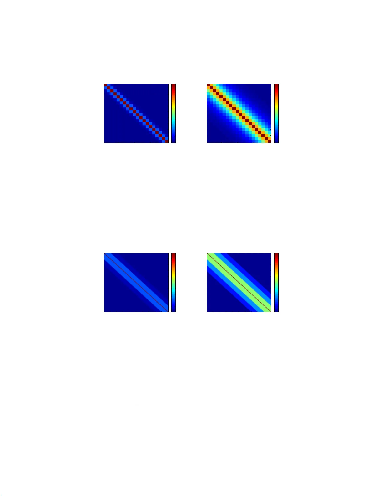
Ultra-high Dimensional Multiple Output Learning With Sim ultaneous Orthogonal Matc hing Pursuit: A Sure S creening Approac h Mladen Kolar and Eric P . Xing Sc ho ol of Computer Science Carnegie Mellon Univ ersity Ma y 27 , 2022 Abstract W e prop os e a no vel application of th e Sim ultaneous Orthogonal Matc h- ing Pursuit (S-OMP) procedu re f or sparsistant v ariable selection in ultra- high dimensional multi-task regression p ro blems. Screening of v ariables, as introduced in F an and Lv (200 8), is an eﬃcien t an d highly scalable w a y to remo ve many irrelev ant va riables from the set of all v ariables, while re- taining all the releva nt v ariables. S-O M P can b e applied to problems with hundreds of thousands of va riables and once th e number of va riables is re- duced to a manageable size, a more compu tatio nally demanding pro cedure can be used to identify the relev ant va riables for eac h of the regression outputs. T o our knowledge, this is the ﬁrst attempt to ut ilize relatedness of multiple outp u ts t o p erf orm fast screening of relev ant v ariables. As our mai n theoretical contri bution, w e pro ve that, asymptotically , S-OMP is guaran teed to reduce an ultra-high n umber of v ariables to b e lo w the sample size without losing true relev ant v ariables. W e also provide for- mal evidence that a mo diﬁed Ba yesi an information criterion (BIC) can b e used to eﬃcien tly determine the num b er of iterations in S -OMP . W e further pro vide empirical evidence on the beneﬁt of v ariable selection us- ing multiple regression outputs join t l y , as opp osed to performing vari able selection for eac h outpu t separately . The ﬁnite sample p erformance of S-OMP is d emo nstrated on extensive sim u l ation studies, and on a genetic association mapping problem. Keywor ds: Adaptive Lasso; Gree dy forw ard regression; Orthogonal matc hing pu rs uit; Multi-outp ut regression; Multi-t a sk learning; Simulta- neous orthogonal matc hing pursuit; Sure screening; V ariable selection 1 In tro duction Multiple output r egression, also known as m ulti-tas k regr ession, with ultr a-high dimensional inputs commonly arise in problems such as genome- wide asso cia- tion (GW A) ma p ping in genetics, or stock p ortfolio pr ediction in ﬁna nce. F or 1 example, in a GW A mapping pr oblem, the goal is to ﬁnd a small set of rele v a n t single-nucleotide p olymorphisms (SNP) ( c ovariates, or input s ) that account for v ariations of a larg e num b er of gene expre ssion or clinical traits ( r esp onses, or outputs ), throug h a respo nse function that is often modeled via a regression. How ever, this is a very challenging problem for current statistica l methods since the num b er o f input v aria ble s is likely to reach millions , pro hibit ing even usag e of s calable implementation o f Lasso- lik e pro cedures for mo del selection, which are a con vex relax ation o f a co m binatorial subse t s election search. F urther more, the outputs in a t y pical multi-task r egression pro blem are not indep enden t of each other, therefore the discov ery of truly re le v a n t inputs has to tak e in to con- sideration of potential joint eﬀects induced by co upled resp onses. T o a pp reciate this b etter, consider a gain the GW A example. Typically , genes in a biolo gical pathw ay ar e co- expressed as a mo dule and it is often as sumed that a causal SNP aﬀects multiple genes in one path wa y , but no t a ll of the g enes in the pathw ay . In order to eﬀectively reduce the dimensionality of the pro blem and to detect the causal SNPs, it is very imp ortant to lo ok at how SNPs aﬀect all ge ne s in a bi- ologica l pathw ay . Since the exp erimen tally collected da t a is usually very noisy , regres s ing genes individually onto SNPs may not b e suﬃcient to identif y the relev ant SNPs that ar e only weakly marginally correlated with ea c h individua l gene in a mo dule. How ever, once the whole bio logical pathw ay is examined, it is muc h e a sier to ﬁnd such caus a l SNPs. In this paper, w e demonstrate that the Sim ultaneous O rthogonal Matching Pursuit (S-OMP) (T r opp et al., 2 006 ) can be used to quickly reduce the dimensiona lit y of such problems, without lo sing any of the relev ant v a riables. F rom a computational point of view, as the dimensio nalit y of the problem and the num b er of outputs incr ease, it can b ecome intractable to so lv e the un- derlying co n vex pro grams commonly used to identif y re lev ant v ar iables in mu lti- task regr ession problems. Pr evious w o rk b y Liu et al. (200 9 ), Lo unici et al. (2009) and Kim et a l. (2009), for example, do not scale well to settings when the num- ber of v ariables exceeds & 1 0 000 and the num b er of o ut puts exceeds & 1 000, as in typical genome-wide asso ciation studies. F urthermor e, since the e stim ation error of the regres sion coe ﬃcie nts dep ends on the num b er of v ar iables in the problem, v ariable selection can improv e co nvergence rates of estima tio n pro ce- dures. These co nc e rns motiv ate us to prop ose and study the S-OMP a s a fast wa y to remov e irrelev ant v a r iables from an ultra- hig h dimensiona l space. F ormally , the GW A mapping problem, which we will use as an illustrative example b oth in here for mo del formulation and later for empirica l exp erimen tal v alidation, can be cast as a v aria ble sele c t ion problem in a multiple output regres s ion mo del: Y = XB + W (1) where Y = [ y 1 , . . . , y T ] ∈ R n × T is a matrix of outputs, whose column y t is an n -vector for the t -th output (i.e., gene), X ∈ R n × p is a random desig n matrix, of which each row x i denotes a p -dimensiona l input, B = [ β 1 , . . . , β T ] ∈ R p × T is the matr ix of regres s ion co eﬃcien ts and W = [ ǫ 1 , . . . , ǫ T ] ∈ R n × T is a matrix of IID random noise, indep enden t o f X . Thr o ughout th e pap er w e a r e g oing to 2 assume that the columns of B ar e jointly spar se, a s w e pre c isely specify b elow. Note that if diﬀerent co lum ns of B do not share any underlying structure , the mo del in (1) can b e estimated by ﬁtting each of the tas k s sepa rately . W e are interested in estimating the r egression co eﬃcien ts, under the as- sumption that they sha re a c o mmon str uctur e, e .g., there exist a subset of v ariables with non-zer o coeﬃcie n ts for more tha n one regr e s sion output. W e informally refer to suc h outputs as r elated. Such a v ariable selection problem can be for ma lized in tw o wa ys: (1) the union supp ort recov e r y of B , as deﬁned in Ob ozinski et al. (20 10 ), where a subset of v aria bles is selected that aﬀect at leas t one output; (2) the exact su p p ort recovery of B , where the exa ct p ositions of non- zero elements in B are estimated. In this pap er, we c o ncern o urselv es with exact suppo rt recovery , which is of particular imp ortance in problems like GW A map- ping (Kim and Xing, 2 009 ) or biologica l netw o rk estimation (Peng et al., 2 008 ). Under such a m ulti-task setting, tw o interesting q ues tions natur a lly follow: i) how c an information b e s hared b et ween r elated outputs in or der to improv e the predictive accuracy and the rate of convergence of the estimated r egression co eﬃcien ts over the indep enden t estimation on each output s e parately; ii) how to select relev ant v aria bles mo re accur ately based on infor ma tion fro m rela ted outputs. T o addr e ss these tw o questions, one line of resear c h (e.g., Zhang, 2006; Liu et al., 200 9 ; Lounici et al., 2009) has lo ok ed into the following estimation pro cedure lev er aging a multi-task r e gularization : ˆ B = argmin β t ∈ R p ,t ∈ [ T ] T X t =1 || y t − X β t || 2 2 + λ p X j =1 pen ( β 1 ,j , . . . , β T ,j ) , (2) with p en( a 1 , . . . , a T ) = max t ∈ [ T ] | a t | o r p en( a 1 , . . . , a T ) = q P t ∈ [ T ] a 2 t for a vector a ∈ R T . Under an appropr iate choice of the p enalt y parameter λ , the es- timator ˆ B ha s many rows equal to zero, which corres pond to irrelev ant v ariables. How ever, s olving (2) ca n be co mput ationally pr ohibitiv e. In this pap er, we consider an ultra-high dimensional setting for the a f ore- men tioned multi-task regr ession problem, where the num b er of v a riables p is m uch higher than the sample size n , e.g. p = O (exp( n δ p )) for a p ositive con- stant δ p , but the reg ression co eﬃcien ts β t are sparse , i.e., for each task t , there exist a very small n umber of v a riables that are relev a nt to the o utput . Under the spar sit y ass um ption, it is highly impor tan t to e ﬃcie n tly se le ct the rele v ant v ariables in order to impro ve the a c c uracy of the estimatio n and prediction, and to fac ilit ate the understanding o f the under lying phenomenon for do ma in ex- per ts. In the semina l paper of F an a nd Lv (20 0 8 ), the conc e pt of su re scr e ening was introduced, which leads to a sequential v ariable selectio n pro cedure that keeps all the relev ant v ariables with high probability in ultra - high dimensional uni-output r e gr ession . In this pap er, we pr opose the S-OMP pro cedure, which enjoys sur e scr e ening proper t y in ultra-high dimensional multiple output r e gr es- sion as deﬁned in (1). T o p erform exact supp ort r eco very , w e further pr opose a tw o-s t ep pro cedure that ﬁrst use S-OMP to screen the v a riables, i.e., select a subset of v a r iables that contain all the true v ariables ; and then use the adap- 3 tive Lasso (ALasso) (Zou, 20 06 ) to further se le c t a subset o f screened v ar ia bles for each task. W e show, both theor etically and empirically , that our pro cedure ensure sparsista n t reco very of relev ant v ar iables. T o the b e s t of o ur knowledge, this is the ﬁrst attempt to analyze the sure screening prope r t y in the ultra-high dimensional space us ing the sha red informatio n from the multiple regre ssion outputs. 1.1 Related W ork The mo del given in (1) has b een use d in many diﬀerent domains rang ing from m ultiv ariate regr ession (Obo zinski et al., 200 9 ; Negahban and W ainwright, 2009) and sparse approximation (T ro pp et a l., 2006) to neura l science (Liu et al., 2 009 ), m ulti-task lear ning (Lounici et al., 20 09 ; Arg y riou et al., 2008) a nd biolo gical net work estima t ion (Peng et al., 2008). A num b er of authors has pro vided the- oretical understanding of the estimation in the mo del using the conv ex prog r am (2) to estimate ˆ B . Lounici et al. (20 09) show ed the b eneﬁts of the joint es tima - tion, when there is a sma ll set of v ariables co m mon to all o utpu ts and the num b er of outputs is lar ge. O bozinski et al. (200 9) and Negahban and W ainwrigh t (200 9 ) analyzed the consis t ent recov e r y of the union supp ort. Nega h ban and W ainwright (2009) provided the analysis of the ex act suppo rt recovery for a spec ial case with tw o outputs. The O rthogonal Matching Pursuit (O MP) has been analyzed b efore in the literature (see, e.g., Z ha ng, 2 009 ; Lozano et al., 20 09 ; W ang, 200 9 ; Barro n et al., 200 8). In particular , our work s hould b e contrasted to W ang (2009), which show ed that the OMP ha s the sure scree nin g pro p erty in a linear regr ession with a single output, and to the exact v ar iable selection pr operty of the O MP analyzed in Zhang (2009) and Lo z ano et al. (200 9 ). The exact v aria ble s election req u ires m uch strong e r as sumpt ions on the design, such a s the irrepresentable condition, that are hard to satisfy in the ultra-hig h dimensio nal setting. On the other hand, the sure scre e nin g prop erty can b e shown to hold under muc h weaker assumptions. In this paper , we make the following nov el cont ributions: i) w e pr o ve that the S-OMP can be used for the ultra-high dimensio n al v ariable scre ening in mul- tiple output regre s sion pro blems and demonstr a te its p erformance on extensive nu merical studies; ii) we show that a tw o s tep pr o cedure can b e used to select exactly the relev ant v ariables for each task; and iii) we prov e that a mo diﬁcation of the BIC scor e (Chen and Chen, 2008) ca n b e used to select the num b er of steps in the S-OMP . The rest of the article is organized as follo ws. In Section 2, w e in tro duce the simult aneous g r eedy fo rw ard regress ion and prop ose our appro ac h to the exact suppo rt estimation. Theoretica l g uaran tees of the metho ds ar e g iv en in Section 3. Section 4 is dev o ted to extensive numerical s im ulations. An applicatio n to the rea l world pro blem in asso ciation mapping is demonstrated in Section 5. W e conclude with discussio n in Section 6 . Pro ofs are deferred to Appendix. 4 2 Metho dology 2.1 The mo del and notation W e will consider a slig h tly more general mo del y 1 = X 1 β 1 + ǫ 1 y 2 = X 2 β 2 + ǫ 2 . . . y T = X T β T + ǫ T , (3) than the one given in (1). The mo del in (1) is a sp ecial case of the mo del in (3), with all the des ign matr ic es { X t } t ∈ [ T ] being equal a nd [ T ] denoting the set { 1 , . . . , T } . Assume that for all t ∈ [ T ], X t ∈ R n × p . F or the desig n X t , we denote X t,j the j -th column (i.e., dimension), x t,i the i -th r o w (i.e., instance) and x t,ij the element a t ( i, j ). Denote Σ t = Cov( x t,i ). Without loss of genera lit y , we a s sume that V ar( y t,i ) = 1 , E ( x t,ij ) = 0 and V ar( x t,ij ) = 1 . The nois e ǫ t is zer o mean and Cov( ǫ t ) = σ 2 I n × n . W e assume tha t the num b er of v a r iables p ≫ n and that the vector of r egression co eﬃcien ts β t are join tly sparse, that is, there ex ist a s m all num b er of v aria bles that are relev ant for the most o f the T regression problems. Put another wa y , the matrix B = [ β 1 , . . . , β T ] has only a small num b er of non-zero rows. Let M ∗ ,t denote the set of non-zero coeﬃcients of β t and M ∗ = ∪ T t =1 M ∗ ,t denote the set of a ll relev a n t v ariables, i.e., v aria bles with non- z ero co eﬃcien t in at least one of the tas k s. F or an arbitr ary set M ⊆ { 1 , . . . , p } , X t, M denotes the desig n with columns indexed by M , B M denotes the rows o f B indexed by M a nd B j = ( β 1 ,j , . . . , β T ,j ) ′ . The car dinalit y of the set M is denoted a s |M| . Let s := |M ∗ | denote the total num b er of relev ant v ariables, s o under the spar sit y assumption we hav e s < n . F or a square matrix A , Λ min ( A ) and Λ max ( A ) are us ed to denote the minim um and the maximum e igen v alue, resp ectively . F or a diﬀerent matrix A = [ a ij ] ∈ R p × T , we deﬁne || A || 2 , 1 := P i ∈ [ p ] q P j ∈ [ T ] a 2 ij . Lastly , w e use [ p ] to denote the set { 1 , . . . , p } . 2.2 Sim ultaneous Ort h ogonal Matchin g Pursuit W e prop ose a Simultaneous Orthog onal Matching Pursuit pro cedure for ultra high-dimensional v aria ble selectio n in the m ulti-ta sk regression problem, which is outlined in Algorithm 1. Before descr ibing the a lgorithm, w e introduce so me additional notation. F o r an ar bitrary subset M ⊆ [ p ] of v ar iables, let H t, M be the or t hogonal pro jection matrix onto Span( X t, M ), i.e., H t, M = X t, M ( X ′ t, M X t, M ) − 1 X ′ t, M , (4) and deﬁne the residual sum of squa res (RSS) as RSS( M ) = T X t =1 y ′ t ( I n × n − H M ) y t . (5) 5 Algorithm 1 Group F o rw ar d Regr ession Input : Dataset { X t , y t } T t =1 Output : S equence of selected models {M ( k ) } n − 1 k =0 1: Set M (0) = ∅ 2: for k = 1 to n − 1 do 3: for j = 1 to p do 4: ˜ M ( k ) j = M ( k − 1) ∪ { j } 5: H t,j = X t, ˜ M ( k ) j ( X ′ t, ˜ M ( k ) j X t, ˜ M ( k ) j ) − 1 X ′ t, ˜ M ( k ) j 6: RSS( ˜ M ( k ) j ) = P T t =1 y ′ t ( I n × n − H t,j ) y t 7: end for 8: ˆ f k = argmin j ∈{ 1 ,...,p }\M ( k − 1) RSS( ˜ M ( k ) j ) 9: M ( k ) = M ( k − 1) ∪ { ˆ f k } 10: end for The algor ithm sta r ts with an empty set M (0) = ∅ . W e recur siv ely deﬁne the set M ( k ) based on the set M ( k − 1) . The set M ( k ) is o bt ained b y adding a v ariable indexed by ˆ f k ∈ [ p ], which minimizes RSS( M ( k − 1) ∪ j ) over the s et [ p ] \M ( k − 1) , to the se t M ( k − 1) . Repeating the algor it hm for n − 1 steps, a sequence of nested sets {M ( k ) } n − 1 k =0 is obtained, with M ( k ) = { ˆ f 1 , . . . , ˆ f k } . T o pra ctically select one of the sets o f v aria ble s from { M ( k ) } n − 1 k =0 , we mini- mize the mo diﬁed BIC criterion (Chen a nd Chen, 200 8 ), w hich is deﬁned as BIC( M ) = log  RSS( M ) nT  + |M| (log( n ) + 2 log( p )) n (6) with |M| deno t ing the num b er of elements of the s e t M . Let ˆ s = argmin k ∈{ 0 ,...,n − 1 } BIC( M ( k ) ) , so that the selected mo del is M ( ˆ s ) . Remark: The S-OMP alg orithm is outlined o nly conceptually in this sec- tion. The steps 5 and 6 of the algor ithm can b e implemented eﬃciently using the progre s siv e Cholesky decomp osition se e, e.g., Cotter et al. (1999). A co m puta- tionally costly step 5 inv olves inversion of the matrix X ′ t, M X t, M , how ever, it can be seen fro m the alg orithm that the matrix X ′ t, M X t, M is up dated in each it- eration b y simply appe nding a row and a co lum n to it. Therefor e , its Cholesky factorization can b e eﬃciently computed based on calculation inv olv ing only the last row. A detailed implementation of the or thogonal matching pursuit algorithm based on the pro gressive Cholesky decomp osition can be found in Rubinstein et al. (2008). 2.3 Exact v ariable selection After removing many o f the irre lev ant v ar iables have b een remov ed using Al- gorithm 1, we are left with the v aria bles in the set M ( ˆ s ) , whose size is smaller 6 than the sample size n . These v ar iables are candidates for the relev ant v aria bles for each of the regr essions. No w, we can a dd ress the pro blem of estimating the regr ession co eﬃcien ts and r eco vering the exa ct supp ort of B using a lo wer dimensional selection pr ocedure. In this pap er, we use the a daptiv e Lasso a s a low er dimensional selectio n procedure, which was sho wn to have oracle proper - ties (Zou, 2006). The ALasso so lv es the p enalized leas t s quare problem ˆ β t = arg m in β t ∈ R ˆ s || y t − X t, M ( ˆ s ) β t || 2 2 + λ X j ∈M ( ˆ s ) w j | β t,j | , (7) where ( w j ) j ∈M ( ˆ s ) is a vector of known weigh t a nd λ is a tuning par ameter. Usually , the weight s are deﬁned as w j = 1 / | ˆ β t,j | where ˆ β t is a √ n -consistent estimator of β t . In a low dimensional setting, we know from Huang et al. (2 0 08) that the adaptive La sso can recover the exactly the r elev ant v aria bles. Therefo re, we can use the ALasso on each output separa tely to recover the ex act suppo rt of B . How ever, in order to ensure that the exa ct s upp ort of B is recov e r ed with high probability , w e need to ha ve that the total num b er o f tasks is o ( n ). The exact supp ort recovery of B is established using the union bo un d over diﬀer- ent tasks, therefore w e need the num b er of tasks to r emain r elativ ely small in compariso n to the s ample size n . How ever, simulation res ult s presented in § ref- sec:simulation sho w that the ALas s o pro cedure succeeds in the exact supp ort recov e r y even when the num b er of tasks are much larger than the sample size, which indica tes that our theoretical considera tions could be impro ved. Figure 1 illustrates the tw o step pr o cedure. ALasso small number of variables Full Model large number of variables S−OMP Screening Exact support Only relevant variables Figure 1: F r amew ork for exa ct suppor r eco very Remark: W e point out that s olving the m ulti-task pr oblem deﬁned in (2) can b e e ﬃcie ntly done o n the reduced set of v ar iables, but it is not obvious how to o bt ain the estimate of the exact supp ort using (2). In Section 4.1, our nu merical studies show that the ALasso applied to the reduced set of v ariables can b e used to estimate the exact supp ort of B . 3 Theory In this sectio n we state conditions under which Algo rithm 1 is sc r eening consis- ten t, i.e., P [ ∃ k ∈ { 0 , 1 , . . . , n − 1 } : M ∗ ⊆ M ( k ) ] → 1 , as n → ∞ . (8) F urthermore, we a lso show that the mo del selected using the mo diﬁed BIC criterion contains all the relev ant v aria bles, i.e., P [ M ∗ ⊆ M ( ˆ s ) ] → 1 , as n → ∞ . (9) 7 Note that we can cho o se trivially M ( n ) since it holds that M ∗ ⊆ M ( n ) . How- ever, we will be able to pr ove that ˆ s chosen by the mo diﬁed BIC criterion is m uch smaller than the sa mp le size n . 3.1 Assumptions Before we state the theo rem characterizing the p erformance of the S-OMP , we give some tec hnica l conditions that a re ne e de d for o ur analysis. A1: The random noise v ectors ǫ 1 , . . . , ǫ T are independent Gaussian with zero mean a n d cov ar iance ma trix σ 2 I n × n . A2: E ac h row of the design matrix X t is IID Gaussian with zero mean and cov aria nce ma trix Σ t . F urther mo re, ther e exist tw o p ositiv e constants 0 < φ min < φ max < ∞ such that φ min ≤ min t ∈ [ T ] Λ min ( Σ t ) ≤ max t ∈ [ T ] Λ max ( Σ t ) ≤ φ max . (10) A3: The true regression co eﬃcien ts are bounded, i.e., there exists a po s it ive constant C β such that || B || 2 , 1 ≤ C β . F urthermor e, the norm of a n y non- zero row of the matrix B is bounded awa y from zero , that is, there exis t po sitiv e cons t ants c β and δ min such that T − 1 min j ∈M ∗ X t ∈ [ T ] β 2 t,j ≥ c β n − δ min . A4: There e x ist p ositiv e cons t ants C s , C p , δ s and δ p such that |M ∗ | ≤ C s n δ s and lo g ( p ) ≤ C p n δ p . The no rmalit y condition A1 is assumed her e o nly to facilitate pres e n tation o f theoretical results, as is c o mmonly assumed in litera ture, (e.g., Zhang and Huang, 20 08 ; F an and Lv, 2008). The no rmalit y assumption c a n b e av oided at the cost of more technical pro ofs, e.g ., Lo unici et al. (20 09 ), where the main tec hnical diﬃ- cult y is showing that the concentration pro perties still hold. Under the condition A2 w e will b e able to show that the empirical cov a riance matrix s a tisﬁes the sparse eigenv alue c ondition (see Lemma 3) with probability tending to o ne. The assumption that the r o ws of the design are Gaussian can b e easily rela xed to the ca se when the r ows a re s ub-Gaussian, without any technical diﬃculties in pro ofs, since w e would still obtain exp onen tial bounds on the tail pro babilities. The conditio n A3 s t ates that the regre s sion co eﬃcients ar e bounded, whic h is a techn ical condition likely to be satisﬁed in pr actice. F urther more, it is assumed that the row norms o f B M ∗ do not decay to zer o to o fas t o r , otherw is e, they would not b e distinguishable from noise. The condition is not too r estrictiv e, e.g., if every non-zer o c o eﬃcient is bo unded aw ay from zero by a constant, the condition A3 is trivia lly satisﬁed with δ min = 0. How ever, we allow the co eﬃ- cients of the re lev ant v a r iables to get smaller as the sample size increas e s and 8 still guarantee that the relev ant v ariable will be identiﬁed. The condition A4 sets the upp er bound on the n umber of relev ant v ariables and the tota l num b er of v a r iables. While the tota l n um ber of v ariables can diverge to inﬁnit y muc h faster than the sa mp le size, the num b er o f relev ant v ar iables needs to b e smaller than the sample size. Conditions A3 and A4 implicitly rela t e diﬀerent out- puts and control the n umber of non-zero co eﬃcien ts shared b et ween diﬀer en t outputs. In tuitiv ely , if the upper b ound in A4 on the s iz e o f M ∗ is large, this immediately implies that the constant C β in A3 sho uld b e lar ge as well, since otherwise there would exist a ro w of B whose ℓ 2 norm would be too small to b e detected by Algorithm 1. 3.2 Screening consistency Our ﬁrst r esults states that after a small num b er o f iteratio ns, compared to the dimensionality p , the S-OMP pro cedure will include a ll the relev ant v ariables. Theorem 1 . A ssume t h e mo del in (3) and that the c onditions A1 - A4 ar e satisﬁe d. F urthermor e, assume t h at n 1 − 6 δ s − 6 δ min max { log( p ) , log( T ) } → ∞ , as n → ∞ . (11) Then t her e exists a n umb er m ∗ max = m ∗ max ( n ) , so that in m ∗ max steps of S-O M P iter ation, al l the r elevant variables ar e include d in t h e mo del, i.e., as n → ∞ P [ M ∗ ⊆ M ( m ∗ max ) ] ≥ 1 − C 1 exp  − C 2 n 1 − 6 δ s − 6 δ min max { log( p ) , log( T ) }  , (12) for some p ositive c onst a nts C 1 and C 2 . The exact value of m ∗ max is given as m ∗ max = ⌊ 2 4 φ − 2 min φ max C 2 β C 2 s c − 2 β n 2 δ s +2 δ min ⌋ . (13) Remarks: Under the assumptions of Theorem 1, m ∗ max ≤ n − 1 , s o that the pro cedure eﬀectiv ely reduces the dimensiona lit y be low the sample siz e . F r o m the pr o of of the theorem, it is clear ho w multiple outputs help to iden tify the relev ant v ar iables. The crucial quantit y in identifying all relev ant v ariables is the minim um no n-zero row nor m of B , which allows us to identify weak v ar i- ables if they a re relev ant for a la rge n um ber of outputs even thoug h individual co eﬃcien ts may b e s m all. It should b e noted that the main improv ement ov er the ordinary forward regr ession is in the seize of the s ignal that can b e de tec ted, as deﬁned in A3 and A4 . Theorem 1 gua r an tees tha t o ne o f the sets {M ( k ) } will contain all re lev ant v ariables, with hig h probability . How ever, it is of practica l imp ortance to se le ct of one se t in the collection that contains all relev ant v aria bles and do es no t hav e to o man y irrelev ant ones. Our following theorem shows that the mo diﬁed BIC criterio n c an be used for this pur pose, that is, the set M ( ˆ s ) is scree ning consistent. 9 Theorem 2. As sume that t he c onditions of The or em 1 ar e satisﬁe d. L et ˆ s = argmin k ∈{ 0 ,... ,n − 1 } BIC( M ( k ) ) (14) b e t h e index of t h e mo del sele cte d by optimizing the mo diﬁe d BIC criterion. Then, as n → ∞ P [ M ∗ ⊆ M ( ˆ s ) ] → 1 . (15) Combining results from Theorem 1 and Theorem 2, we have shown that the S-OMP pro cedure is screening consistent and can be applied to problems wher e the dimensionality of the problem p is exp onen tial in the num b er of observed samples. In the next section, we also show that the S-OMP has great empirical per formance. 4 Numerical studies In this section w e p erform sim ulation studies on an extensive num b er syn thetic data sets. F urthermor e, we demons t rate the application of the pro cedure on the genome-wide asso ciation mapping problem. 4.1 Sim ulation studies W e c o nduct an extensive num b er of numerical studies to ev aluate the ﬁnite sample per formance of the S-OMP . W e consider three pro cedures that p erform estimation on individuals outputs: Sure Indep endence Screening (SIS), Iterative SIS (ISIS) (F an and Lv, 2008), and the OMP , for compa r ison purp oses. The ev aluation is do ne on the mo del in (1). SIS and ISIS a re use d to selec t a subset of v ariables a nd then the ALas so is used to further reﬁne the selection. W e denote this combination as SIS- ALa sso and ISIS-ALass o. The size of the mo del selected by SIS is ﬁxed as n − 1, while the ISIS selects ⌊ n/ log( n ) ⌋ v a riables in each of the ⌊ log( n ) − 1 ⌋ itera t ions. F r om the screened v ariables , the ﬁnal mo del is selected using the ALasso, together with the BIC criterion (6) to determine the pena lt y parameter λ . The num b er of v ariables selected by the O MP is determined using the B IC criterion, how ever, we do not fur ther reﬁne the se le cted v ariables us ing the ALasso, since from the numerical studies in W ang (20 09 ) it was observed that the further reﬁnement do es not r e sult in improv ement . The S- OMP is used to r e duce the dimensio nalit y below the sa mple siz e jointly using the regr ession outputs. Next, the ALas s o is used on ea c h of the o u tputs to further p erform the estimation. This combination is denoted SOMP -ALasso. Let ˆ B = [ ˆ β 1 , . . . , ˆ β T ] ∈ R p × T be an estimate obtained by o ne of the esti- mation pro cedures. W e ev aluate the per f ormance av eraged ov er 200 simulation runs. Let ˆ E n denote the empir ical av er age ov er the simulation runs. W e measure the s ize o f the union supp ort ˆ S = S ( ˆ B ) := { j ∈ [ p ] : || ˆ B j || 2 2 > 0 } . Nex t, we es t i- mate the pr obabilit y that the s creening pro perty is satisﬁed ˆ E n [1 I {M ∗ ⊆ S ( ˆ B ) } ], which we call cov er a ge proba bilit y . F or the union suppor t , we deﬁne frac- tion of correc t zero s ( p − s ) − 1 ˆ E n [ | S ( ˆ B ) C ∩ M C ∗ | ], fra ction o f incor rect zeros 10 s − 1 ˆ E n [ | S ( ˆ B ) C ∩ M ∗ | ] and fraction o f co rrectly ﬁtted ˆ E n [1 I {M ∗ = S ( ˆ B ) } ] to measure the p erformance of diﬀer en t pro cedures. Simila r quantities a re deﬁned for the exa ct suppo rt recov e r y . In addition, we measure the estimation error ˆ E n [ || B − ˆ B || 2 2 ] and the prediction perfor mance on the test set. On the test data { x ∗ i , y ∗ i } i ∈ [ n ] , we compute R 2 = 1 − P i ∈ [ n ] P t ∈ [ T ] ( y ∗ t,i − ( x ∗ t,i ) ′ ˆ β t ) 2 P i ∈ [ n ] P t ∈ [ T ] ( y ∗ t,i − ¯ y ∗ t ) 2 , (16) where ¯ y ∗ t = n − 1 P i ∈ [ n ] y t,i . The following simulation studies are used to compara tiv ely a s sess the n u- merical p erformance of the pro cedures. Due to space co nstrain ts, tables with detailed n umer ical res ults are given in the app endix. In this section, w e outline main ﬁndings. Simulation 1: [Mo del with uncor related v aria bles] The following toy mo del is based on the simulation I in F an a nd Lv (2008) with ( n, p, s, T ) = (400 , 2000 0 , 18 , 500). Each x i is drawn indep enden tly fro m a standard m ultiv a riate normal distribu- tion, so that the v a riables are mutu ally indepe ndent. F or j ∈ [ s ] and t ∈ [ T ], the non-zero co eﬃcien ts of B are given as β t,j = ( − 1) u (4 n − 1 / 2 log n + | z | ), where u ∼ Bernoulli(0 . 4) and z ∼ N (0 , 1). The num b er of non-zero elements in B j is giv en as a par ameter T non − zero ∈ { 500 , 300 , 100 } . The p o sitions of non-zero elements are c hos en uniformly at random from [ T ]. The noise is Gaussian with the standar d devia t ion σ set to control the s ignal-to-noise ratio (SNR). SNR is deﬁned as V a r ( x β ) / V ar( ǫ ) and we v ar y SNR ∈ { 15 , 10 , 5 , 1 } . Simulation 2 : [Changing the num b er of non-zero e le m ent s in B j ] The follow- ing scenar io is used to ev aluate the p erformance of the metho ds as the num b er of non-zero element s in a row of B v arie s. W e set ( n, p, s ) = (100 , 500 , 1 0) and v ary the num b er of outputs T ∈ { 50 0 , 750 , 1000 } . F o r each num b er of out- puts T , we v a ry T non − zero ∈ { 0 . 8 T , 0 . 5 T , 0 . 2 T } . The samples x i and r e gression co eﬃcien ts B are given as in Simulation 1 , i.e ., x i is drawn from a multiv ari- ate standard norma l distribution and the non-ze r o co eﬃcien ts B are g iven as β t,j = ( − 1) u (4 n − 1 / 2 log n + | z | ), where u ∼ Bernoulli(0 . 4) and z ∼ N (0 , 1). The noise is Gaus sian, with the standard deviation deﬁned through the SNR, whic h v aries in { 1 0 , 5 , 1 } . Simulation 3: [Mo del with the decaying co r relation be tw een v aria bles] The following mo del is bor ro wed from W ang (200 9 ). W e as sume a corr elation str uc- ture b et ween v ariables given as V ar( X j 1 , X j 2 ) = ρ | j 1 − j 2 | , whe r e ρ ∈ { 0 . 2 , 0 . 5 , 0 . 7 } . This correla t ion structur e app ears natura lly among ordered v ariables. W e set ( n, p , s, T ) = (100 , 5000 , 3 , 15 0) a nd T non − zero = 8 0. The relev ant v a riables a re at po sitions (1 , 4 , 7) and non-zero co eﬃcien ts are given as 3 , 1 . 5 a nd 2 resp ec- tively . The SNR v arie s in { 10 , 5 , 1 } . A heat map of the cor relation matr ix betw een diﬀerent cov aria tes is given in Figure 2. Simulation 4: [Model with the blo c k-co mpound correla t ion structure] The following mo del assumes a blo c k compo un d correlation structure . F or a para m- eter ρ , the co rrelation betw e en t wo v ariables X j 1 and X j 2 is giv en a s ρ , ρ 2 or ρ 3 when | j 1 − j 2 | ≤ 10, | j 1 − j 2 | ∈ (10 , 2 0 ] or | j 1 − j 2 | ∈ (20 , 30] and it is set 11 5 10 15 20 2 4 6 8 10 12 14 16 18 20 0.1 0.2 0.3 0.4 0.5 0.6 0.7 0.8 0.9 1 (a) ρ = 0 . 2 5 10 15 20 2 4 6 8 10 12 14 16 18 20 0.1 0.2 0.3 0.4 0.5 0.6 0.7 0.8 0.9 1 (b) ρ = 0 . 7 Figure 2: Visualization of the cor relation matrix in Sim ulation 3. Only an upp er left corne r is presented corres ponding to 20 of the 500 0 v ar iables. to 0 otherwise. W e set ( n, p, s, T ) = (150 , 40 00 , 8 , 150), T non − zero = 80 a nd the parameter ρ ∈ { 0 . 2 , 0 . 5 } . The relev ant v ariables are a t lo cated at positio ns 1, 11, 21, 31, 41, 5 1, 61, 71 a nd 8 1, so that e a c h blo c k of highly correla ted v ariables has exactly one relev ant v a riable. The v alues o f relev ant co eﬃcien ts is given as in Sim ulation 1. The noise is Gaussian and the SNR v aries in { 10 , 5 , 1 } . A heat map of the corr elation matrix betw een diﬀerent cov a riates is given in Figure 3. 10 20 30 40 50 60 70 80 90 100 10 20 30 40 50 60 70 80 90 100 0 0.1 0.2 0.3 0.4 0.5 0.6 0.7 0.8 0.9 1 (a) ρ = 0 . 2 10 20 30 40 50 60 70 80 90 100 10 20 30 40 50 60 70 80 90 100 0 0.1 0.2 0.3 0.4 0.5 0.6 0.7 0.8 0.9 1 (b) ρ = 0 . 5 Figure 3: Visualization of the cor relation matrix in Sim ulation 4. Only an upp er left corne r is presented corres ponding to 100 of the 4000 v ar iables. Simulation 5: [Mo del with a ’masked’ relev ant v ariable] This mo del r epre- sents a diﬃcult s ett ing. It is mo diﬁed from W ang (2009). W e set ( n, p, s, T ) = (200 , 10000 , 5 , 500). The num b er of no n-zero elements in each row v aries is T non − zero ∈ { 4 00 , 25 0 , 100 } . F or j ∈ [ s ] and t ∈ [ T ], the non-zero elements equal β t,j = 2 j . Each row of X is gener ated a s follows. Draw independently z i and z ′ i from a p -dimensional standard m ultiv ar iate nor ma l distribution. No w, x ij = ( z ij + z ′ ij ) / p (2) for j ∈ [ s ] and x ij = ( z ij + P j ′ ∈ [ s ] z ij ′ ) / 2 for j ∈ [ p ] \ [ s ]. Now, Corr( x i, 1 , y t,i ) is m uch smaller then Corr( x i,j , y t,i ) for j ∈ [ p ] \ [ s ], so that it 12 bec omes diﬃcult to select v ar iable 1 . The v ariable 1 is ’ma s k ed’ with the nois y v ariables. This s e t ting is diﬃcult for scree n ing pr ocedures a s they take into consideratio n only marg inal information. The noise is Gaus sian with standard deviation σ ∈ { 1 . 5 , 2 . 5 , 4 . 5 } . In the next section we summarize r esults of our exp erimental ﬁndings. Our simulation setting transitions from a simple scenar io co nsidered in Simulation 1 tow ards a challenging one in Sim ulation 5 . Simulation 1 is a do pted from F an and Lv (2008) as a toy mo del on which all algo rithms should work w ell. Sim ulation 2 exa mines the inﬂuence of the n umber of non-zero elemen ts in a relev ant r o w o f the matrix B . W e exp ect that Algor it hm 1 will o utp er- form pro cedures that perfor m estimatio n on individual outputs when T non − zero is larg e, while when T non − zero is small the single-tas k scr e ening pro cedures should have an adv antage. Our intuition is als o suppo rted by recent res ult s of Kolar et al. (201 0 ). Sim ulations 3 and 4 repr esen t more challenging situa- tions with structur ed corr e lation tha t natur ally app ears in many data sets, for example, a co rrelation b et ween gene measur emen ts that ar e clos ely lo cated on a chromosome. Finally Sim ula t ion 5 is constr uc ted in such a way that procedures which use only marginal informa t ion are go ing to include irr elev ant v a riables befo re relev ant o nes. 4.2 Results of sim ulations T ables giv ing detailed results of the ab o ve describ ed simulations are given in the Appendix. In this section, we outline main ﬁndings and repro duce some parts of the tables that we think a re insigh tful. T able 1 shows parts of the res ults fo r simulation 1 . W e can se e that all metho d s perfor m well in the setting when the input v aria bles a r e mutually uncorrela t ed and the SNR is high. Note that even though the v ariables ar e uncorrela t ed, the sample cor relation betw een v aria bles c an b e quite high due to large p and small n , which can result in selection o f spur ious v aria bles. As we can see from the table, comparing to SIS, ISIS and OMP , the S-OMP is a ble to select the co rrect union supp ort, while the proc e du res that select v ar iables bas e d on diﬀerent outputs separately also include a ddit ional spurious v ar iables int o the selection. F urthermore, we c a n see that the S-OMP -ALasso pro cedure do es m uch b etter o n the problem of exact suppo rt re c overy c o mpared to the other pro cedures. The ﬁr st simulations sugg ests that so mewhat higher computatio na l cost of the S-OMP pro cedure can b e justiﬁed by the improv ed perfor mance on the pro blem of union and exa ct suppor t recov ery as well as o n the erro r in the estimated co eﬃcien ts. T able 2 shows parts of the results for simulation 2. In this simulation w e measured the p erformance o f e s tim ation pro cedures as the amount of shared input v ariable s be t ween diﬀerent outputs v aries. The parameter T non − zero con- trols the a m ount of information that is shared betw een diﬀerent tasks as deﬁned in the previous subsection. In particular , the parameter controls the num b er of non-zero elements in a row o f the matrix B corres p onding to a relev ant v ariable. When the n umber of non-z e ro elements is high, a v ar iable is relev ant to many 13 T able 1: Results for simulation 1 with parameters ( n, p, s, T ) = (500 , 2 0000 , 1 8 , 500), T non − zero = 500 Prob. ( %) of F raction (%) of F raction (%) of F raction (%) of Est. e r ror T est err or Method name M ∗ ⊆ ˆ S Correct zeros Incorrect zeros M ∗ = ˆ S | ˆ S | || B − ˆ B || 2 2 R 2 SNR = 15 Union Support SIS-ALASSO 100.0 100.0 0.0 10.0 20.2 - - ISIS-ALASSO 100.0 100.0 0.0 18.0 19.6 - - OMP 100.0 100.0 0.0 0.0 23.9 - - S-OMP 100.0 100.0 0.0 100.0 18.0 - - S-OMP-ALASSO 100.0 100.0 0.0 100.0 18.0 - - Exact Support SIS-ALASSO 0.0 100.0 0.7 0.0 8940.5 0.97 0.93 ISIS-ALASSO 100.0 100.0 0.0 18.0 9001.6 0.33 0.93 OMP 100.0 100.0 0.0 0.0 9005.9 0.20 0.93 S-OMP-ALASSO 100.0 100.0 0.0 100.0 9000.0 0.20 0.93 T able 2: Results for simulation 2 with parameters ( n, p, s, T ) = (20 0 , 5000 , 10 , 1000), T non − zero = 2 00 Prob. ( %) of F raction (%) of F raction (%) of F raction (%) of Est. e r ror T est err or Method name M ∗ ⊆ ˆ S Correct zeros Incorrect zeros M ∗ = ˆ S | ˆ S | || B − ˆ B || 2 2 R 2 SNR = 5 Union Support SIS-ALASSO 100.0 100.0 0.0 100.0 10.0 - - ISIS-ALASSO 100.0 100.0 0.0 100.0 10.0 - - OMP 100.0 97.4 0.0 0.0 139.6 - - S-OMP 100.0 100.0 0.0 100.0 10.0 - - S-OMP-ALASSO 100.0 100.0 0.0 100.0 10.0 - - Exact Support SIS-ALASSO 100.0 100.0 0.0 100.0 2000.0 0.04 0.72 ISIS-ALASSO 100.0 100.0 0.0 100.0 2000.0 0.04 0.72 OMP 100.0 100.0 0.0 0.0 2131.6 0.05 0.71 S-OMP-ALASSO 100.0 100.0 0.0 100.0 2000.0 0.03 0.72 T able 3: Results for simulation 3 with parameters ( n, p, s, T ) = (100 , 5 000 , 3 , 150), T non − zero = 80, ρ = 0 . 5 Prob. ( %) of F raction (%) of F raction (%) of F raction (%) of Est. e r ror T est err or Method name M ∗ ⊆ ˆ S Correct zeros Incorrect zeros M ∗ = ˆ S | ˆ S | || B − ˆ B || 2 2 R 2 SNR = 5 Union Support SIS-ALASSO 100.0 100.0 0.0 97.0 3.0 - - ISIS-ALASSO 100.0 100.0 0.0 96.0 3.0 - - OMP 100.0 99.8 0.0 0.0 19.6 - - S-OMP 100.0 100.0 0.0 100.0 3.0 - - S-OMP-ALASSO 100.0 100.0 0.0 100.0 3.0 - - Exact Support SIS-ALASSO 60.0 100.0 0.2 57.0 239.5 0.10 0.61 ISIS-ALASSO 84.0 100.0 0.1 80.0 239.8 0.08 0.61 OMP 100.0 100.0 0.0 0.0 256.6 0.06 0.61 S-OMP-ALASSO 100.0 100.0 0.0 100.0 240.0 0.03 0.62 14 T able 4: Results of simulation 4 with parameter s ( n, p, s, T ) = (15 0 , 400 0 , 8 , 150), T non − zero = 80, ρ = 0 . 5 Prob. ( %) of F raction (%) of F raction (%) of F raction (%) of Est. e r ror T est err or Method name M ∗ ⊆ ˆ S Correct zeros Incorrect zeros M ∗ = ˆ S | ˆ S | || B − ˆ B || 2 2 R 2 SNR = 10 Union Support SIS-ALASSO 100.0 100.0 0.0 100.0 8.0 - - ISIS-ALASSO 100.0 100.0 0.0 97.0 8.0 - - OMP 100.0 99.9 0.0 2.0 11.7 - - S-OMP 100.0 100.0 0.0 100.0 8.0 - - S-OMP-ALASSO 100.0 100.0 0.0 100.0 8.0 - - Exact Support SIS-ALASSO 35.0 100.0 1.4 35.0 631.3 0.55 0.88 ISIS-ALASSO 100.0 100.0 0.0 97.0 640.0 0.14 0.89 OMP 100.0 100.0 0.0 2.0 643.7 0.10 0.89 S-OMP-ALASSO 100.0 100.0 0.0 100.0 640.0 0.09 0.89 T able 5: Results of simulation 5 with parameter s ( n, p, s, T ) = (20 0 , 100 0 0 , 5 , 500), T non − zero = 400 Prob. ( %) of F raction (%) of F raction (%) of F raction (%) of Est. e r ror T est err or Method name M ∗ ⊆ ˆ S Correct zeros Incorrect zeros M ∗ = ˆ S | ˆ S | || B − ˆ B || 2 2 R 2 σ = 1.5 Union Support SIS-ALASSO 53.0 99.6 9.4 0.0 41.1 - - ISIS-ALASSO 100.0 99.8 0.0 0.0 28.1 - - OMP 100.0 99.9 0.0 12.0 10.0 - - S-OMP 100.0 100.0 0.0 44.0 5.6 - - S-OMP-ALASSO 100.0 100.0 0.0 100.0 5.0 - - Exact Support SIS-ALASSO 0.0 100.0 68.9 0.0 936.0 84.66 0.66 ISIS-ALASSO 0.0 100.0 16.2 0.0 1791 .9 5.80 0.96 OMP 100.0 100.0 0.0 12.0 2090.3 0.06 0.99 S-OMP-ALASSO 100.0 100.0 0.0 100.0 2000.0 0.05 0.99 15 tasks and we say that outputs overlap. In this setting the S-O MP pro cedure is exp ected to outp e rform the other metho ds, howev er, when T non − zero is lo w, the no ise coming from the tasks for which the v ar ia ble is irrelev ant can actually harm the pe r formance. The table sho ws results when the overlap of sha red v ari- ables is small, that is, a r elev ant v ariable is o nly r elev ant for 1 0% of outputs. As one could ex pect, the S-OMP pr o cedure do es as w ell as other pro cedures. This is no t surprising, since the amount of shared info r mation b et ween diﬀer- ent o utputs is limited. Therefor e, if one exp ects little v aria ble sharing acros s diﬀerent outputs, using the SIS or ISIS may results in similar acc ur acy , but a n improv ed computational eﬃciency . It is worth pointing out that in our simu- lations, the diﬀerent tasks are correlated since the same design X used for all tasks. Ho wever, we expect the same qualitative r esults even under the mo de l given in equation (3) where diﬀerent tasks c an hav e diﬀere n t des ig ns X t and the outputs are uncorre lated. Sim ulation 3 represents a s it uation that commonly o ccur in nature, where there is an o r dering amo n g input v ariables and the correlatio n be tw een v aria ble s decays as the distance b et ween v ar iables incr ease. The mo del in s im ulation 4 is a mo diﬁcation of the mo del in simu lation 3 where the v aria bles are group ed and there is s ome correla tion betw een diﬀer en t groups . T a ble 3 gives r esults for simulation 3 for the parameter ρ = 0 . 5 . In this s ett ing, the S-O MP per- forms mu ch better that the other pro cedures. The improvemen t beco mes more pronounced with inc r ease of the cor r elation pa rameter ρ . Similar behavior is observed in sim ulation 4 as well, see table 4. Results of simulation 5, g iv en in T able 5, further re info r ce o ur intuit ion that the S-OMP pro cedure do es well even on problems with high-cor relation betw een the set o f relev ant input v aria bles and the se t of irrelev ant ones. T o further compare the p erformance of the S-OMP pro cedure to the SIS, w e explore the minimum num b er of iteratio ns needed for the a lgorithm to include all the relev ant v aria bles into the selected mo del. F rom o ur limited n umerical exp erience, we note that the simulation parameters do no t aﬀect the num b er of iterations for the S-OMP proce dur e. This is unlike the SIS pr ocedure, whic h o ccasionally requires a large num b er of steps b efore all the true v aria bles ar e included, see Figure 3 in F an a nd Lv (2008). W e no t e that while the S-OMP pro cedure do es include, in man y cases, all the relev ant v ariables b efore the irrelev ant ones, the BIC criterion is not able to corr e c t ly select the num b er of v ariables to include, when the SNR is small. As a r esult, we can see the drop in p erformance as the SNR decreas es. 4.3 Real data analysis W e demonstra te an a pplication of the S-OMP to a genome-wide a ssociation mapping problem. The data were collected b y o ur colla borator Judie Howry- lak, M.D. at Ha r v ard Medic a l Scho ol from 200 individuals that ar e s uﬀ e r ing from as thma . F or eac h individual, w e hav e a collection of a bout ∼ 35000 0 ge- 16 netic markers 1 , whic h are ca lled sing le n ucleotide p olymorphisms (SNPs), and a collectio n of 14 24 g ene expressio n meas uremen ts. The goal of this study is to identify a small num ber of SNPs that can he lp explain v ariatio n s in gene expressions . Typically , this type of ana lysis is done by regressing each gene in- dividually o n the mea sured SNPs, howev er, since the data are very noisy , such an approa c h results selecting many v aria bles. O ur approach to this pr oblem here is to regres s a group of genes onto the SNPs instea d. Ther e ha s b een so me previous work on this problem Kim a nd Xing (2009), that considered regre s s- ing groups of genes onto SNPs, how ever, tho s e approaches use v ariants of the estimation pro cedure given in Eq. (2), whic h is not easily sca lable to the data we analyze here. W e use the s p ectral rela xation of the k-means clustering Zha et al. (2 001) to group 14 24 genes into 48 clusters acco rding to their expre s sion v alues, so that the minim um, maximum and median num b er o f genes p er cluster is 4, 90 and 1 9, resp ectiv ely . The num b er of clusters was chosen somewha t arbitrarily , based on the domain knowledge of the medical exp erts. The main idea b ehind the clustering is that we wan t to identify genes that b elong to the same regulator y pathw ay since they ar e mor e likely to b e a ﬀ ected with the s a me SNPs. Instead of clustering, one may use prior kno wledg e to identify in teres tin g groups of genes. Next, w e wan t to use the S-O MP pro cedure to iden tify relev ant SNPs for each of the gene clusters. Since, w e do no t ha ve the ground truth for the data set, w e use pr e dic tive p o wer on the test set a nd the size of estimated mo dels to acce ss their q ualit y . W e r a ndomly split the data into a training set of size 170 and a testing set of size 30 and re p ort results ov er 500 runs. W e compute the R 2 co eﬃcien t on the tes t set deﬁned as 1 − 3 0 − 1 T − 1 P t ∈ [ T ] || y t, test − X t, test ˆ β t || 2 2 (beca use the data has b een nor m alized). Due to s pa ce co nstrain ts, we g ive results on few cluster s in T able 6 a nd note that, qualitativ ely , the results do not v ar y muc h betw een diﬀeren t clusters. While the ﬁtted mo dels have limited predictive p erformance, which res ults from highly noisy da ta, we obs e rv e that the S-OMP is able to identify on a verage one SNP p er gene cluster that is rela t ed to a larg e num b er of g enes. Other metho ds, while having a similar predictive p erformance, select a la rger num b er of SNPs which can b e seen from the size o f the union supp ort. O n this pa rticular da ta set, the S-O MP seems pro duce results that a r e mor e interpretable from a sp ecialist’s po in ts of view. F urther inv estiga t ion needs to be done to v er if y the biolo gical signiﬁcance of the selected SNPs, how ever, the details of such a n analy sis are going to be rep orted elsewhere. 5 Conclusions In this w ork, we analyze the Simultaneous O rthogonal Matching Purs uit a s a metho d for v ariable selection in an ultra-high dimensio na l space. W e prov e that the S-O MP is screening consistent and provide a practical wa y to select the 1 These mark ers w ere preprocessed, by imputing missing v alues and remo ving duplicate SNPs that were p e rfectly correlated wi th other SNPs. 17 T able 6 : Results on the asthma data Method name Union support R 2 Cluster 9 Size = 18 SIS-ALASSO 18.0 (1.0) 0.178 (0.006) OMP 1 7.5 (2.9) 0.167 (0.002) S-OMP 1.0 (0.0) 0.214 (0.005) Cluster 16 Size = 31 SIS-ALASSO 31.0 (1.0) 0.160 (0.007) OMP 2 9.0 (1.8) 0.165 (0.002) S-OMP 1.0 (0.0) 0.209 (0.005) Cluster 17 Size = 19 SIS-ALASSO 18.5 (0.9) 0.173 (0.006) OMP 1 9.5 (0.8) 0.146 (0.003) S-OMP 1.0 (0.0) 0.184 (0.004) Cluster 19 Size = 17 SIS-ALASSO 17.0 (1.2) 0.270 (0.017) OMP 1 1.0 (4.1) 0.213 (0.008) S-OMP 1.0 (0.0) 0.280 (0.017) Cluster 22 Size = 34 SIS-ALASSO 34.0 (0.9) 0.153 (0.005) OMP 3 0.0 (7.3) 0.142 (0.000) S-OMP 1.0 (0.0) 0.145 (0.002) Cluster 23 Size = 35 SIS-ALASSO 35.0 (0.9) 0.238 (0.018) OMP 3 3.0 (9.9) 0.208 (0.009) S-OMP 1.0 (0.0) 0.229 (0.014) Cluster 24 Size = 28 SIS-ALASSO 28.0 (1.0) 0.123 (0.003) OMP 2 8.0 (2.6) 0.114 (0.001) S-OMP 1.0 (0.0) 0.129 (0.003) Cluster 32 Size = 15 SIS-ALASSO 15.0 (0.9) 0.188 (0.010) OMP 1 0.0 (2.6) 0.211 (0.006) S-OMP 1.0 (0.0) 0.215 (0.008) Cluster 36 Size = 33 SIS-ALASSO 34.0 (1.4) 0.147 (0.005) OMP 2 9.0 (5.3) 0.157 (0.002) S-OMP 1.0 (0.0) 0.168 (0.004) Cluster 37 Size = 19 SIS-ALASSO 19.0 (0.9) 0.207 (0.015) OMP 2 2.0 (2.5) 0.175 (0.006) S-OMP 1.0 (0.0) 0.235 (0.014) Cluster 39 Size = 24 SIS-ALASSO 24.0 (0.9) 0.131 (0.006) OMP 2 7.0 (1.9) 0.141 (0.003) S-OMP 1.0 (0.0) 0.160 (0.005) Cluster 44 Size = 35 SIS-ALASSO 35.0 (0.9) 0.177 (0.010) OMP 2 6.5 (6.6) 0.183 (0.005) S-OMP 1.0 (0.0) 0.170 (0.011) Cluster 49 Size = 23 SIS-ALASSO 23.0 (1.0) 0.124 (0.004) OMP 2 3.0 (1.2) 0.140 (0.000) S-OMP 1.0 (0.0) 0.159 (0.004) 18 nu mber of steps in the pro ce dur e us ing the mo diﬁed Bayesian infor mation crite- rion. Our limited n umerical exp erience sho ws that the metho d pe rforms w ell in practice and that the joint estimation from m ultiple o utputs often outp erforms metho ds that use one reg ression output at the time. F urthermo r e, w e can see the S-OMP procedur e as w ay to impro ve the v a riable selec tio n pro p e rties of the SIS without ha ving to solve a costly complex optimization pro cedure in Eq. (2 ), therefore, balancing the computationa l costs a nd the estimatio n acc ur acy . 6 App endix 6.1 Pro of of Theorem 1 Under the a ssumptions of the theor em, the num b er of r elev ant v aria bles s is relatively small c o mpared to the sa mple size n . The pro o f strategy can b e outlined as follo ws: i) w e are going to sho w that, with high probabilit y , at least one relev ant v aria ble is going to be identiﬁed within the following m ∗ one steps, conditioning on the already selected v ariables M ( k ) and this holds uniformly for all k ; ii) we can conclude that all the relev ant v ariables are going to be selected within m ∗ max = sm ∗ one steps. Exa ct v alues fo r m ∗ one and m ∗ max are given b elow. Without loss o f genera lity , we a nalyze the ﬁrst step o f the a lgorithm, i.e., we show that the ﬁrst relev ant v ar iable is going to be selected within the ﬁrst m ∗ one steps. Assume that in the ﬁrst m ∗ one − 1 steps, there were no r e le v ant v ariables selected. Assuming that the v ariable sele cted in the m ∗ one -th step is still an irrelev ant one, we will a rrive at a con tradiction, which shows that at lea st one relev ant v aria ble has b een selected in the ﬁrst m ∗ one steps. F or a ny step k , the reduction of the squared error is g iven as ∆( k ) := RSS( k − 1) − RSS( k ) = X t || H ( k ) t, ˆ f k ( I n × n − H t, M ( k ) ) y t || 2 2 (17) with H ( k ) t,j = X ( k ) t,j X ( k ) ′ t,j || X ( k ) t,j || − 2 and X ( k ) t,j = ( I n × n − H t, M ( k ) ) X t,j . W e a re int erested in the quant it y P m ∗ one k =1 ∆( k ), when all the s elected v ariables ˆ f k (see Algorithm 1) b elo ng to [ p ] \ M ∗ . In what follows, we will der ive a lower b ound for ∆( k ). W e p erform our analysis on the even t E = { min t ∈ [ T ] min M⊆ [ p ] , |M|≤ m ∗ max Λ min ( ˆ Σ M ) ≥ φ min / 2 } \ { max t ∈ [ T ] max M⊆ [ p ] , |M|≤ m ∗ max Λ max ( ˆ Σ M ) ≤ 2 φ max } . (18) 19 F rom the deﬁnition of ˆ f k , we hav e ∆( k ) ≥ max j ∈M ∗ X t || H ( k ) t,j ( I n × n − H t, M ( k ) ) y t || 2 2 ≥ max j ∈M ∗  X t || H ( k ) t,j ( I n × n − H t, M ( k ) ) X t, M ∗ β t, M ∗ || 2 2 − X t || H ( k ) t,j ( I n × n − H t, M ( k ) ) ǫ t || 2 2  ≥ max j ∈M ∗ X t || H ( k ) t,j ( I n × n − H t, M ( k ) ) X t, M ∗ β t, M ∗ || 2 2 − max j ∈M ∗ X t || H ( k ) t,j ( I n × n − H t, M ( k ) ) ǫ t || 2 2 = ( I ) − ( I I ) . (19) W e deal with these tw o terms separa tely . Let H ⊥ t, M = I n × n − H t, M denote the pro jection matrix . W e hav e that the ﬁrst term ( I ) is low er b ounded by max j ∈M ∗ X t || H ( k ) t,j H ⊥ t, M ( k ) X t, M ∗ β t, M ∗ || 2 2 = max j ∈M ∗ X t || X ( k ) t,j || − 2 2 | X ( k ) ′ t,j H ⊥ t, M ( k ) X t, M ∗ β t, M ∗ | 2 ≥ min t ∈ [ T ] ,j ∈M ∗ {|| X ( k ) t,j || − 2 2 } max j ∈M ∗ X t | X ( k ) ′ t,j H ⊥ t, M ( k ) X t, M ∗ β t, M ∗ | 2 ≥ { max t ∈ [ T ] ,j ∈M ∗ || X t,j || 2 2 } − 1 max j ∈M ∗ X t | X ′ t,j H ⊥ t, M ( k ) X t, M ∗ β t, M ∗ | 2 , (20) where the la st inequality follows from the fact that || X t,j || 2 ≥ || X ( k ) t,j || 2 and X ( k ) ′ t,j H ⊥ t, M ( k ) = X ′ t,j H ⊥ t, M ( k ) . A simple ca lc ulation shows that X t || H ⊥ t, M ( k ) X t, M ∗ β t, M ∗ || 2 2 = X t X j ∈M ∗ β t,j X t,j H ⊥ t, M ( k ) X t, M ∗ β t, M ∗ ≤ X j ∈M ∗ s X t β 2 t,j s X t ( X t,j H ⊥ t, M ( k ) X t, M ∗ β t, M ∗ ) 2 ≤ || β || 2 , 1 max j ∈M ∗ s X t ( X t,j H ⊥ t, M ( k ) X t, M ∗ β t, M ∗ ) 2 . (21) Plugging (21) back in to (20), the following lo wer bo und is achiev ed ( I ) ≥ { max t ∈ [ T ] ,j ∈M ∗ || X t,j || 2 2 } − 1 ( P t || H ⊥ t, M ( k ) X t, M ∗ β t, M ∗ || 2 2 ) 2 || B || 2 2 , 1 . (22) 20 On the even t E , max t ∈ [ T ] ,j ∈M ∗ || X t,j || 2 2 ≤ 2 nφ max . Since we have assumed that no additional relev ant predictor s have be e n selected by the pro cedure, it holds that M ∗ 6⊆ M ( k ) . This leads to X t || H ⊥ t, M ( k ) X t, M ∗ β t, M ∗ || 2 2 ≥ 2 − 1 nφ min min j ∈M ∗ X t ∈ [ T ] β 2 t,j , (23) on the ev ent E . Using the Cauch y-Sch warz inequality , || B || − 2 2 , 1 ≥ s − 1 T − 1 C − 2 β . Plugging back into (22), w e hav e that ( I ) ≥ 2 − 3 φ 2 min φ − 1 max C − 2 β ns − 1 T − 1 ( min j ∈M ∗ X t ∈ [ T ] β 2 t,j ) 2 ≥ 2 − 3 φ 2 min φ − 1 max C − 2 β C − 1 s n 1 − δ s T − 1 ( min j ∈M ∗ X t ∈ [ T ] β 2 t,j ) 2 (24) Next, we dea l with the s econd term in (1 9). Recall that X ( k ) t,j = H ⊥ t, M ( k ) X t,j , so that || X ( k ) t,j || 2 2 ≥ 2 − 1 nφ min , on the even t E . W e hav e X t || H ( k ) t,j ( I n × n − H t, M ( k ) ) ǫ t || 2 2 = X t || X ( k ) t,j || − 2 ( X ′ t,j H ⊥ t, M ( k ) ǫ t ) 2 ≤ 2 φ − 1 min n − 1 max j ∈M ∗ max |M|≤ m ∗ max X t ( X ′ t,j H ⊥ t, M ǫ t ) 2 . (25) Under the conditions of the theorem, X ′ t,j H ⊥ t, M ǫ t is normally distributed with mean 0 and v ariance || H ⊥ t, M X t,j || 2 2 . F urthermore, max j ∈M ∗ max |M|≤ m ∗ max max t ∈ [ T ] || H ⊥ t, M X t,j || 2 2 ≤ 2 nφ max . (26) Plugging back in (25), w e hav e ( I I ) ≤ 2 2 φ − 1 min φ max max j ∈M ∗ max |M|≤ m ∗ max χ 2 T , (27) where χ 2 T denotes a chi-squared rando m v ariable with T degrees of freedom. The to tal n umber of poss ibilities for j ∈ M ∗ and |M| ≤ m ∗ max is bounded b y p m ∗ max +2 . Using L e mma 5, with ǫ = T ( m ∗ max + 2) log p and applying the union bo und, we obtain ( I I ) ≤ 2 3 φ − 1 min φ max T ( m ∗ max + 2) log p ≤ 9 φ − 1 min φ max C p n δ p T m ∗ max (28) with proba bility at least 1 − p m ∗ max +2 exp − 2 T ( m ∗ max + 2) log( p ) 1 − 2 s 1 2( m ∗ max + 2) log( p ) !! . (29) 21 Going back to (19), we ha ve the following n − 1 T − 1 ∆( k ) ≥ 2 − 3 φ 2 min φ − 1 max C − 2 β C − 1 s n − δ s T − 2 ( min j ∈M ∗ X t ∈ [ T ] β 2 t,j ) 2 − 9 φ − 1 min φ max C p n δ p − 1 m ∗ max ≥ 2 − 3 φ 2 min φ − 1 max C − 2 β C − 1 s c 2 β n − δ s − 2 δ min − 9 φ − 1 min φ max C p n δ p − 1 m ∗ max ≥ 2 − 3 φ 2 min φ − 1 max C − 2 β C − 1 s c 2 β n − δ s − 2 δ min × (1 − 72 φ − 3 min φ 2 max C 2 β C p C s c − 2 β n δ s +2 δ min + δ p − 1 m ∗ max ) . (30) Since the b ound in (30) holds unifor mly fo r k ∈ { 1 , . . . , m ∗ one } , we have that n − 1 T − 1 P t ∈ [ T ] || y t || 2 2 ≥ n − 1 T − 1 P m ∗ one k =1 ∆( k ). Setting m ∗ one = ⌊ 2 4 φ − 2 min φ max C 2 β C s c − 2 β n δ s +2 δ min ⌋ (31) and recalling that m ∗ max = sm ∗ one , the low er b ound beco mes n − 1 T − 1 X t ∈ [ T ] || y t || 2 2 ≥ 2(1 − C n 3 δ s +4 δ min + δ p − 1 ) , (32) for a p ositive constant C independent of p, n, s a nd T . Under the conditions of the theorem, the right side of (32) is b ounded b elow by 2. W e have arrived at a con tr a diction, s ince under the as s umptions V ar ( y t,i ) = 1 and by the weak la w of large num b ers, n − 1 T − 1 P t ∈ [ T ] || y t || 2 2 → 1 in probability . Therefore, at least one relev ant v ariable will b e selected in m ∗ one steps. T o co mplete the pro of, we low e r bo und the probabilit y in (2 8) and the pro b- ability o f the ev ent E . P lugging in the v alue for m ∗ max , the probability in (28) can b e low er bounded by 1 − exp( − C (2 T − 1) n 2 δ s +2 δ min + δ p ) for some p ositive constant C . The probability of the event E is low er bounded, using Lemma 3 together with the union b o und, as 1 − C 1 exp( − C 2 n 1 − 6 δ s − 6 δ min max { log p, log T } ), for s ome p os- itive constants C 1 and C 2 . Bo th of these probabilities conv er ge to 1 under the conditions of the theorem. 6.2 Pro of of Theorem 2 T o prov e the theorem, we use the same str ategy as in W ang (2009). F ro m Theorem 1, we hav e that P [ ∃ k ∈ { 0 , . . . , n − 1 } : M ∗ ⊆ M ( k ) ] → 1, so k min := min k ∈{ 0 ,... ,n − 1 } { k : M ∗ ⊆ M ( k ) } is well deﬁned and k min ≤ m ∗ max , for m ∗ max deﬁned in (13). W e show that P [ min k ∈{ 0 ,...,k min − 1 } (BIC( M ( k ) ) − BIC( M ( k +1) )) > 0] → 1 , (33) 22 so that P [ ˆ s < k min ] → 0 as n → ∞ . W e pro ceed by low er b o unding the diﬀerence in the BIC scores a s BIC( M ( k ) ) − BIC( M ( k +1) ) = log  RSS( M ( k ) ) RSS( M ( k +1) )  − log( n ) + 2 log( p ) n ≥ log  1 + RSS( M ( k ) ) − RSS( M ( k +1) ) RSS( M ( k +1) )  − 3 n − 1 log( p ) , (34) where we ha ve a ssumed p > n . Deﬁne the event A := { n − 1 T − 1 P t ∈ [ T ] || y t || 2 2 ≤ 2 } . Note that RSS( M ( k +1) ) ≤ P t ∈ [ T ] || y t || 2 2 , so on the even t A the diﬀerence in the BIC scores is low er b ounded as log(1 + 2 n − 1 T − 1 ∆( k )) − 3 n − 1 log( p ) , (35) where ∆( k ) is deﬁned in (17). Using the fact that log(1 + x ) ≥ min(log (2) , 2 − 1 x ) and the lower bound fro m (30), we ha ve BIC( M ( k ) ) − BIC( M ( k +1) ) ≥ min(log 2 , C n − δ s − 2 δ min ) − 3 n − 1 log p, (3 6) for some p ositive c o nstant C . It is easy to chec k that lo g 2 − 3 n − 1 log p > 0 and C n − δ s − 2 δ min − 3 n − 1 log p > 0 under the conditions of the theor em. The low er bo und in (36) is uniform for k ∈ { 0 , . . . , k min } , so the pr o of is complete if we show that P [ A ] → 1. But this ea sily follo ws from the tail bo unds on the central chi-squared random v ariable given in Lemma 4. 6.3 Collection of kno wn results In what follows, C 1 , C 2 , . . . will denote arbitrar y positive constants. The fo llowing r esult on the minim um eigenv alue of sub-matrices of the co- v ariance matrix ˆ Σ is quite standar d (e.g. Zhou et al. (200 9), W a ng (200 9) or Bick el et a l. (20 0 9)). Lemma 3. L et x ∼ N (0 , Σ ) and ˆ Σ = n − 1 P n i =1 x i x ′ i b e the empiric al estimate fr om n indep endent r e alizations of x . Denote Σ = [ σ ab ] and ˆ Σ = [ ˆ σ ab ] . Assume φ min ≤ Λ min ( Σ ) ≤ Λ max ( Σ ) ≤ φ max . Then P [ max M⊆ [ p ] , |M| n , P [ max i ∈ [ m ] X i ≥ 2 ǫ ] ≤ m exp( − ǫ (1 − 2 r n ǫ )) . (41) 24 25 6.4 T ables with simu lation results Simulati on 1: ( n, p, s, T ) = ( 500 , 20000 , 18 , 500 ), T non − zero = 500 Method name M ∗ ⊆ ˆ S Correct zero s Incorrect zeros M ∗ = ˆ S | ˆ S | || B − ˆ B || 2 2 R 2 SNR = 15 Union Supp ort SIS-A LA SSO 100.0 100.0 0.0 10.0 20.2 - - ISIS-A LASSO 100.0 100.0 0.0 18. 0 19.6 - - OMP 100.0 100.0 0.0 0.0 23.9 - - S-OMP 100.0 100.0 0.0 100.0 18.0 - - S-OMP-ALAS SO 100 .0 100.0 0.0 1 00.0 18.0 - - Exact Supp ort SIS-A LA SSO 0.0 100.0 0.7 0.0 8940.5 0.9 7 0.93 ISIS-A LASSO 100.0 100.0 0.0 18. 0 9001.6 0.33 0.93 OMP 100.0 100.0 0.0 0.0 9005.9 0.20 0.93 S-OMP-ALAS SO 100 .0 100.0 0.0 1 00.0 9000.0 0.20 0.93 SNR = 10 Union Supp ort SIS-A LA SSO 100.0 100.0 0.0 0.0 25.3 - - ISIS-A LASSO 100.0 100.0 0.0 0.0 25.7 - - OMP 100.0 100.0 0.0 0.0 23.9 - - S-OMP 100.0 100.0 0.0 100.0 18.0 - - S-OMP-ALAS SO 100 .0 100.0 0.0 1 00.0 18.0 - - Exact Supp ort SIS-A LA SSO 0.0 100.0 1.6 0.0 8861.0 2.0 6 0.89 ISIS-A LASSO 100.0 100.0 0.0 0.0 9007.7 0.65 0.90 OMP 100.0 100.0 0.0 0.0 9005.9 0.31 0.91 S-OMP-ALAS SO 65. 0 100. 0 0.1 65.0 8987. 4 0.41 0.90 SNR = 5 Union Supp ort SIS-A LA SSO 100.0 100.0 0.0 64.0 18.4 - - ISIS-A LASSO 100.0 100.0 0.0 57. 0 18.6 - - OMP 100.0 100.0 0.0 0.0 24.0 - - S-OMP 100.0 100.0 0.0 100.0 18.0 - - S-OMP-ALAS SO 100 .0 100.0 0.0 1 00.0 18.0 - - Exact Supp ort SIS-A LA SSO 0.0 100.0 92.8 0.0 6 45.8 74. 61 0.06 ISIS-A LASSO 0.0 100.0 90.9 0.0 822.2 73 .06 0.07 OMP 100.0 100.0 0.0 0.0 9006.0 0.61 0.83 S-OMP-ALAS SO 0.0 100.0 70.3 0.0 2668.9 56.65 0.24 SNR = 1 Union Supp ort SIS-A LA SSO 0.0 100.0 99.9 0.0 0.0 - - ISIS-A LASSO 0.0 100.0 100.0 0.0 0.0 - - OMP 100.0 100.0 0.0 0.0 25.9 - - S-OMP 0.0 100.0 94.4 0.0 1.0 - - S-OMP-ALAS SO 0.0 100.0 99.0 0.0 0.2 - - Exact Supp ort SIS-A LA SSO 0.0 100.0 100.0 0.0 0.0 80.27 -0.00 ISIS-A LASSO 0.0 100.0 100.0 0.0 0.0 80.27 -0.00 OMP 0.0 100.0 86.5 0.0 1222.8 71.40 0.05 S-OMP-ALAS SO 0.0 100.0 100.0 0.0 0.2 80.27 -0.00 26 Simulati on 1: ( n, p, s, T ) = ( 500 , 20000 , 18 , 500 ), T non − zero = 300 Method name M ∗ ⊆ ˆ S Correct zero s Incorrect zeros M ∗ = ˆ S | ˆ S | || B − ˆ B || 2 2 R 2 SNR = 15 Union Supp ort SIS-A LA SSO 100.0 100.0 0.0 97.0 18.0 - - ISIS-A LASSO 100.0 100.0 0.0 98. 0 18.0 - - OMP 100.0 100.0 0.0 0.0 23.0 - - S-OMP 100.0 100.0 0.0 100.0 18.0 - - S-OMP-ALAS SO 100 .0 100.0 0.0 1 00.0 18.0 - - Exact Supp ort SIS-A LA SSO 55 .0 100 .0 0.0 53.0 5399. 3 0.10 0.93 ISIS-A LASSO 100.0 100.0 0.0 98. 0 5400.0 0.09 0.93 OMP 100.0 100.0 0.0 0.0 5405.0 0.07 0.93 S-OMP-ALAS SO 100 .0 100.0 0.0 1 00.0 5400.0 0.07 0.93 SNR = 10 Union Supp ort SIS-A LA SSO 100.0 100.0 0.0 82.0 18.2 - - ISIS-A LASSO 100.0 100.0 0.0 91. 0 18.1 - - OMP 100.0 100.0 0.0 0.0 23.0 - - S-OMP 100.0 100.0 0.0 100.0 18.0 - - S-OMP-ALAS SO 100 .0 100.0 0.0 1 00.0 18.0 - - Exact Supp ort SIS-A LA SSO 42 .0 100 .0 0.0 33.0 5399. 2 0.18 0.90 ISIS-A LASSO 100.0 100.0 0.0 91. 0 5400.1 0.16 0.90 OMP 100.0 100.0 0.0 0.0 5405.0 0.11 0.90 S-OMP-ALAS SO 100 .0 100.0 0.0 1 00.0 5400.0 0.11 0.90 SNR = 5 Union Supp ort SIS-A LA SSO 100.0 100.0 0.0 3.0 21.1 - - ISIS-A LASSO 100.0 100.0 0.0 6.0 20.8 - - OMP 100.0 100.0 0.0 0.0 23.0 - - S-OMP 100.0 100.0 0.0 100.0 18.0 - - S-OMP-ALAS SO 100 .0 100.0 0.0 1 00.0 18.0 - - Exact Supp ort SIS-A LA SSO 24 .0 100 .0 0.0 1.0 5400.9 0.61 0.82 ISIS-A LASSO 99.0 1 00.0 0.0 6.0 5402.8 0.52 0.82 OMP 100.0 100.0 0.0 0.0 5405.0 0.22 0.82 S-OMP-ALAS SO 100 .0 100.0 0.0 1 00.0 5400.0 0.23 0.82 SNR = 1 Union Supp ort SIS-A LA SSO 0.0 100.0 97.9 0.0 0.4 - - ISIS-A LASSO 0.0 100.0 97.9 0.0 0.4 - - OMP 100.0 100.0 0.0 0.0 25.9 - - S-OMP 0.0 100.0 94.4 0.0 1.0 - - S-OMP-ALAS SO 0.0 100.0 94.4 0.0 1.0 - - Exact Supp ort SIS-A LA SSO 0.0 100.0 100.0 0.0 0.4 48.16 -0.00 ISIS-A LASSO 0.0 100.0 100.0 0.0 0.4 48.16 -0.00 OMP 0.0 100.0 10.2 0.0 4858.1 5.76 0.43 S-OMP-ALAS SO 0.0 100.0 99.9 0.0 6.1 48.12 -0.00 27 Simulati on 1: ( n, p , s, T ) = (500 , 200 00 , 18 , 500), T non − zero = 100 Method name M ∗ ⊆ ˆ S Correct zero s Incorrect zeros M ∗ = ˆ S | ˆ S | || B − ˆ B || 2 2 R 2 SNR = 15 Union Supp ort SIS-A LA SSO 100.0 100.0 0.0 100.0 18.0 - - ISIS-A LASSO 100.0 100.0 0.0 100.0 18.0 - - OMP 100.0 99. 9 0.0 0.0 2 8.8 - - S-OMP 100.0 100.0 0.0 100.0 18.0 - - S-OMP-ALAS SO 100 .0 100.0 0.0 1 00.0 18.0 - - Exact Supp ort SIS-A LA SSO 100.0 100.0 0.0 100.0 1800.0 0.0 1 0.9 1 ISIS-A LASSO 100.0 100.0 0.0 100.0 1800.0 0.01 0.91 OMP 100.0 100.0 0.0 0.0 1810.8 0.01 0.91 S-OMP-ALAS SO 100 .0 100.0 0.0 1 00.0 1800.0 0.01 0.91 SNR = 10 Union Supp ort SIS-A LA SSO 100.0 100.0 0.0 100.0 18.0 - - ISIS-A LASSO 100.0 100.0 0.0 100.0 18.0 - - OMP 100.0 99. 9 0.0 0.0 2 8.8 - - S-OMP 100.0 100.0 0.0 100.0 18.0 - - S-OMP-ALAS SO 100 .0 100.0 0.0 1 00.0 18.0 - - Exact Supp ort SIS-A LA SSO 100.0 100.0 0.0 100.0 1800.0 0.0 1 0.88 ISIS-A LASSO 100.0 100.0 0.0 100.0 1800.0 0.01 0.88 OMP 100.0 100.0 0.0 0.0 1810.8 0.01 0.88 S-OMP-ALAS SO 100 .0 100.0 0.0 1 00.0 1800.0 0.01 0.88 SNR = 5 Union Supp ort SIS-A LA SSO 100.0 100.0 0.0 100.0 18.0 - - ISIS-A LASSO 100.0 100.0 0.0 100.0 18.0 - - OMP 100.0 99. 9 0.0 0.0 2 8.8 - - S-OMP 100.0 100.0 0.0 100.0 18.0 - - S-OMP-ALAS SO 100 .0 100.0 0.0 1 00.0 18.0 - - Exact Supp ort SIS-A LA SSO 100.0 100.0 0.0 100.0 1800.0 0.0 4 0.79 ISIS-A LASSO 100.0 100.0 0.0 100.0 1800.0 0.03 0.79 OMP 100.0 100.0 0.0 0.0 1810.8 0.03 0.79 S-OMP-ALAS SO 100 .0 100.0 0.0 1 00.0 1800.0 0.02 0.79 SNR = 1 Union Supp ort SIS-A LA SSO 100.0 100.0 0.0 19.0 19.6 - - ISIS-A LASSO 100.0 100.0 0.0 35. 0 19.0 - - OMP 100.0 99. 9 0.0 0.0 2 8.8 - - S-OMP 0.0 100.0 94.4 0.0 1.0 - - S-OMP-ALAS SO 0.0 100.0 94.4 0.0 1.0 - - Exact Supp ort SIS-A LA SSO 59 .0 100 .0 0.0 10.0 1800. 9 0.74 0.45 ISIS-A LASSO 89.0 1 00.0 0.0 32.0 1800.8 0.63 0.45 OMP 100.0 100.0 0.0 0.0 1810.8 0.13 0.47 S-OMP-ALAS SO 0.0 100.0 95.3 0.0 84. 6 15.31 0.02 28 Simulati on 2.a: ( n, p, s, T ) = (200 , 5000 , 10 , 500), T non − zero = 400 Method name M ∗ ⊆ ˆ S Correct zero s Incorrect zeros M ∗ = ˆ S | ˆ S | || B − ˆ B || 2 2 R 2 SNR = 10 Union Supp ort SIS-A LA SSO 100.0 100.0 0.0 39.0 10.9 - - ISIS-A LASSO 100.0 100.0 0.0 12. 0 12.2 - - OMP 100.0 99. 8 0.0 0.0 2 1.6 - - S-OMP 100.0 100.0 0.0 100.0 10.0 - - S-OMP-ALAS SO 100 .0 100.0 0.0 1 00.0 10.0 - - Exact Supp ort SIS-A LA SSO 0.0 100.0 6.4 0.0 3746.6 3.58 0.85 ISIS-A LASSO 41.0 1 00.0 0.2 3.0 3992.8 0.53 0.90 OMP 100.0 100.0 0.0 0.0 4011.7 0.22 0.90 S-OMP-ALAS SO 99. 0 100. 0 0.0 98.0 3999. 9 0.22 0.90 SNR = 5 Union Supp ort SIS-A LA SSO 100.0 100.0 0.0 45.0 11.0 - - ISIS-A LASSO 100.0 100.0 0.0 37. 0 10.9 - - OMP 100.0 99. 8 0.0 0.0 2 2.2 - - S-OMP 100.0 100.0 0.0 100.0 10.0 - - S-OMP-ALAS SO 100 .0 100.0 0.0 1 00.0 10.0 - - Exact Supp ort SIS-A LA SSO 0.0 100.0 65.9 0.0 1363.5 33.32 0.30 ISIS-A LASSO 0.0 100.0 63.1 0.0 1477.0 31.89 0.33 OMP 100.0 100.0 0.0 0.0 4012.2 0.45 0.82 S-OMP-ALAS SO 0.0 100.0 48.0 0.0 2081.5 24.19 0.46 SNR = 1 Union Supp ort SIS-A LA SSO 0.0 100.0 98.2 0.0 0.2 - - ISIS-A LASSO 0.0 100.0 98.7 0.0 0.1 - - OMP 100.0 99. 5 0.0 0.0 3 5.2 - - S-OMP 0.0 100.0 90.0 0.0 1.0 - - S-OMP-ALAS SO 0.0 100.0 95.4 0.0 0.5 - - Exact Supp ort SIS-A LA SSO 0.0 100.0 100.0 0.0 0.2 49.94 -0.00 ISIS-A LASSO 0.0 100.0 100.0 0.0 0.1 49.94 -0.00 OMP 0.0 100.0 76.5 0.0 964.4 40.05 0.09 S-OMP-ALAS SO 0.0 100.0 100.0 0.0 0.8 49.94 -0.00 29 Simulati on 2.a: ( n, p, s, T ) = (200 , 5000 , 10 , 500), T non − zero = 250 Method name M ∗ ⊆ ˆ S Correct zero s Incorrect zeros M ∗ = ˆ S | ˆ S | || B − ˆ B || 2 2 R 2 SNR = 10 Union Supp ort SIS-A LA SSO 100.0 100.0 0.0 99.0 10.0 - - ISIS-A LASSO 100.0 100.0 0.0 98. 0 10.0 - - OMP 100.0 99. 8 0.0 0.0 1 9.9 - - S-OMP 100.0 100.0 0.0 100.0 10.0 - - S-OMP-ALAS SO 100 .0 100.0 0.0 1 00.0 10.0 - - Exact Supp ort SIS-A LA SSO 22 .0 100 .0 0.2 22.0 2495. 4 0.19 0.89 ISIS-A LASSO 100.0 100.0 0.0 98. 0 2500.0 0.12 0.89 OMP 100.0 100.0 0.0 0.0 2509.9 0.09 0.90 S-OMP-ALAS SO 100 .0 100.0 0.0 1 00.0 2500.0 0.08 0.90 SNR = 5 Union Supp ort SIS-A LA SSO 100.0 100.0 0.0 44.0 10.8 - - ISIS-A LASSO 100.0 100.0 0.0 46. 0 10.8 - - OMP 100.0 99. 8 0.0 0.0 1 9.9 - - S-OMP 100.0 100.0 0.0 100.0 10.0 - - S-OMP-ALAS SO 100 .0 100.0 0.0 1 00.0 10.0 - - Exact Supp ort SIS-A LA SSO 12 .0 100 .0 0.9 6.0 2479.5 0.69 0.80 ISIS-A LASSO 62.0 1 00.0 0.2 29.0 2496.7 0.43 0.81 OMP 100.0 100.0 0.0 0.0 2509.9 0.18 0.81 S-OMP-ALAS SO 95. 0 100. 0 0.0 95.0 2499. 6 0.18 0.81 SNR = 1 Union Supp ort SIS-A LA SSO 0.0 100.0 65.3 0.0 3.5 - - ISIS-A LASSO 0.0 100.0 61.3 0.0 3.9 - - OMP 100.0 99. 7 0.0 0.0 2 4.7 - - S-OMP 0.0 100.0 90.0 0.0 1.0 - - S-OMP-ALAS SO 0.0 100.0 90.0 0.0 1.0 - - Exact Supp ort SIS-A LA SSO 0.0 100.0 99.8 0.0 4.6 3 1.16 -0.00 ISIS-A LASSO 0.0 100.0 99.8 0.0 5.2 31.15 - 0.00 OMP 0.0 100.0 17.2 0.0 2083.7 6.09 0.39 S-OMP-ALAS SO 0.0 100.0 99.6 0.0 10. 4 31.11 - 0.00 30 Simulati on 2.a: ( n, p, s, T ) = (200 , 50 00 , 10 , 500), T non − zero = 100 Method name M ∗ ⊆ ˆ S Correct zero s Incorrect zeros M ∗ = ˆ S | ˆ S | || B − ˆ B || 2 2 R 2 SNR = 10 Union Supp ort SIS-A LA SSO 100.0 100.0 0.0 100.0 10.0 - - ISIS-A LASSO 100.0 100.0 0.0 100.0 10.0 - - OMP 100.0 98. 8 0.0 0.0 6 9.8 - - S-OMP 100.0 100.0 0.0 100.0 10.0 - - S-OMP-ALAS SO 100 .0 100.0 0.0 1 00.0 10.0 - - Exact Supp ort SIS-A LA SSO 98 .0 100 .0 0.0 98.0 1000. 0 0.02 0.80 ISIS-A LASSO 100.0 100.0 0.0 100.0 1000.0 0.01 0.80 OMP 100.0 100.0 0.0 0.0 1060.2 0.02 0.79 S-OMP-ALAS SO 100 .0 100.0 0.0 1 00.0 1000.0 0.01 0.80 SNR = 5 Union Supp ort SIS-A LA SSO 100.0 100.0 0.0 100.0 10.0 - - ISIS-A LASSO 100.0 100.0 0.0 100.0 10.0 - - OMP 100.0 98. 8 0.0 0.0 6 9.8 - - S-OMP 100.0 100.0 0.0 100.0 10.0 - - S-OMP-ALAS SO 100 .0 100.0 0.0 1 00.0 10.0 - - Exact Supp ort SIS-A LA SSO 98 .0 100 .0 0.0 98.0 1000. 0 0.04 0.73 ISIS-A LASSO 100.0 100.0 0.0 100.0 1000.0 0.04 0.73 OMP 100.0 100.0 0.0 0.0 1060.2 0.05 0.72 S-OMP-ALAS SO 100 .0 100.0 0.0 1 00.0 1000.0 0.03 0.73 SNR = 1 Union Supp ort SIS-A LA SSO 100.0 100.0 0.0 61.0 10.6 - - ISIS-A LASSO 100.0 100.0 0.0 60. 0 10.5 - - OMP 100.0 98. 8 0.0 0.0 6 9.8 - - S-OMP 0.0 100.0 90.0 0.0 1.0 - - S-OMP-ALAS SO 0.0 100.0 90.0 0.0 1.0 - - Exact Supp ort SIS-A LA SSO 0.0 100.0 12.7 0.0 873.9 2.23 0.37 ISIS-A LASSO 0.0 100.0 9.8 0.0 902.8 1.79 0.38 OMP 100.0 100.0 0.0 0.0 1060.2 0.25 0.42 S-OMP-ALAS SO 0.0 100.0 93.3 0.0 67. 4 11.66 0.03 31 Simulati on 2.b: ( n, p, s , T ) = (200 , 5000 , 10 , 750), T non − zero = 600 Method name M ∗ ⊆ ˆ S Correct zero s Incorrect zeros M ∗ = ˆ S | ˆ S | || B − ˆ B || 2 2 R 2 SNR = 10 Union Supp ort SIS-A LA SSO 100.0 100.0 0.0 25.0 11.3 - - ISIS-A LASSO 100.0 99. 9 0.0 5.0 1 3.3 - - OMP 100.0 99. 7 0.0 0.0 2 6.6 - - S-OMP 100.0 100.0 0.0 100.0 10.0 - - S-OMP-ALAS SO 100 .0 100.0 0.0 1 00.0 10.0 - - Exact Supp ort SIS-A LA SSO 0.0 100.0 6.9 0.0 5585.0 3.87 0.84 ISIS-A LASSO 29.0 1 00.0 0.3 4.0 5986.6 0.56 0.90 OMP 100.0 100.0 0.0 0.0 6016.7 0.22 0.90 S-OMP-ALAS SO 91. 0 100. 0 0.0 91.0 5999. 1 0.23 0.90 SNR = 5 Union Supp ort SIS-A LA SSO 100.0 100.0 0.0 27.0 11.4 - - ISIS-A LASSO 100.0 100.0 0.0 28. 0 11.3 - - OMP 100.0 99. 7 0.0 0.0 2 7.3 - - S-OMP 100.0 100.0 0.0 100.0 10.0 - - S-OMP-ALAS SO 100 .0 100.0 0.0 1 00.0 10.0 - - Exact Supp ort SIS-A LA SSO 0.0 100.0 66.5 0.0 2011.9 33.60 0.30 ISIS-A LASSO 0.0 100.0 63.6 0.0 2185.7 32.14 0.32 OMP 100.0 100.0 0.0 0.0 6017.5 0.45 0.82 S-OMP-ALAS SO 0.0 100.0 48.3 0.0 3104.4 24.34 0.45 SNR = 1 Union Supp ort SIS-A LA SSO 0.0 100.0 97.8 0.0 0.2 - - ISIS-A LASSO 0.0 100.0 98.2 0.0 0.2 - - OMP 100.0 99. 2 0.0 0.0 4 7.6 - - S-OMP 0.0 100.0 90.0 0.0 1.0 - - S-OMP-ALAS SO 0.0 100.0 94.7 0.0 0.5 - - Exact Supp ort SIS-A LA SSO 0.0 100.0 100.0 0.0 0.2 49.94 -0.01 ISIS-A LASSO 0.0 100.0 100.0 0.0 0.2 49.94 -0.01 OMP 0.0 100.0 76.7 0.0 1436.7 40.13 0.09 S-OMP-ALAS SO 0.0 100.0 100.0 0.0 1.0 49.94 -0.01 32 Simulati on 2.b: ( n, p, s , T ) = (200 , 5000 , 10 , 750), T non − zero = 375 Method name M ∗ ⊆ ˆ S Correct zero s Incorrect zeros M ∗ = ˆ S | ˆ S | || B − ˆ B || 2 2 R 2 SNR = 10 Union Supp ort SIS-A LA SSO 100.0 100.0 0.0 99.0 10.0 - - ISIS-A LASSO 100.0 100.0 0.0 93. 0 10.1 - - OMP 100.0 99. 7 0.0 0.0 2 4.7 - - S-OMP 100.0 100.0 0.0 100.0 10.0 - - S-OMP-ALAS SO 100 .0 100.0 0.0 1 00.0 10.0 - - Exact Supp ort SIS-A LA SSO 16 .0 100 .0 0.2 16.0 3741. 3 0.21 0.89 ISIS-A LASSO 100.0 100.0 0.0 93. 0 3750.1 0.12 0.89 OMP 100.0 100.0 0.0 0.0 3764.8 0.09 0.89 S-OMP-ALAS SO 100 .0 100.0 0.0 1 00.0 3750.0 0.09 0.89 SNR = 5 Union Supp ort SIS-A LA SSO 100.0 100.0 0.0 41.0 10.9 - - ISIS-A LASSO 100.0 100.0 0.0 25. 0 11.4 - - OMP 100.0 99. 7 0.0 0.0 2 4.7 - - S-OMP 100.0 100.0 0.0 100.0 10.0 - - S-OMP-ALAS SO 100 .0 100.0 0.0 1 00.0 10.0 - - Exact Supp ort SIS-A LA SSO 6.0 100.0 1.0 3.0 3713.5 0.73 0.80 ISIS-A LASSO 53.0 1 00.0 0.2 13.0 3744.9 0.43 0.80 OMP 100.0 100.0 0.0 0.0 3764.8 0.18 0.81 S-OMP-ALAS SO 91. 0 100. 0 0.0 91.0 3749. 0 0.19 0.81 SNR = 1 Union Supp ort SIS-A LA SSO 0.0 100.0 55.8 0.0 4.4 - - ISIS-A LASSO 1.0 100.0 52.8 1.0 4.7 - - OMP 100.0 99. 6 0.0 0.0 3 2.0 - - S-OMP 0.0 100.0 90.0 0.0 1.0 - - S-OMP-ALAS SO 0.0 100.0 90.0 0.0 1.0 - - Exact Supp ort SIS-A LA SSO 0.0 100.0 99.8 0.0 6.6 3 1.16 -0.00 ISIS-A LASSO 0.0 100.0 99.8 0.0 7.3 31.16 - 0.00 OMP 0.0 100.0 17.6 0.0 3111.8 6.21 0.39 S-OMP-ALAS SO 0.0 100.0 99.6 0.0 15. 1 31.11 - 0.00 33 Simulati on 2.b: ( n, p, s , T ) = (200 , 5000 , 10 , 750 ), T non − zero = 150 Method name M ∗ ⊆ ˆ S Correct zero s Incorrect zeros M ∗ = ˆ S | ˆ S | || B − ˆ B || 2 2 R 2 SNR = 10 Union Supp ort SIS-A LA SSO 100.0 100.0 0.0 100.0 10.0 - - ISIS-A LASSO 100.0 100.0 0.0 100.0 10.0 - - OMP 100.0 98. 0 0.0 0.0 108.5 - - S-OMP 100.0 100.0 0.0 100.0 10.0 - - S-OMP-ALAS SO 100 .0 100.0 0.0 1 00.0 10.0 - - Exact Supp ort SIS-A LA SSO 98 .0 100 .0 0.0 98.0 1500. 0 0.02 0.79 ISIS-A LASSO 100.0 100.0 0.0 100.0 1500.0 0.02 0.79 OMP 100.0 100.0 0.0 0.0 1599.5 0.03 0.78 S-OMP-ALAS SO 100 .0 100.0 0.0 1 00.0 1500.0 0.01 0.79 SNR = 5 Union Supp ort SIS-A LA SSO 100.0 100.0 0.0 100.0 10.0 - - ISIS-A LASSO 100.0 100.0 0.0 100.0 10.0 - - OMP 100.0 98. 0 0.0 0.0 108.5 - - S-OMP 100.0 100.0 0.0 100.0 10.0 - - S-OMP-ALAS SO 100 .0 100.0 0.0 1 00.0 10.0 - - Exact Supp ort SIS-A LA SSO 98 .0 100 .0 0.0 98.0 1500. 0 0.04 0.72 ISIS-A LASSO 100.0 100.0 0.0 100.0 1500.0 0.04 0.72 OMP 100.0 100.0 0.0 0.0 1599.5 0.05 0.71 S-OMP-ALAS SO 100 .0 100.0 0.0 1 00.0 1500.0 0.03 0.72 SNR = 1 Union Supp ort SIS-A LA SSO 100.0 100.0 0.0 46.0 10.8 - - ISIS-A LASSO 100.0 100.0 0.0 42. 0 10.8 - - OMP 100.0 98. 0 0.0 0.0 108.5 - - S-OMP 0.0 100.0 90.0 0.0 1.0 - - S-OMP-ALAS SO 0.0 100.0 90.0 0.0 1.0 - - Exact Supp ort SIS-A LA SSO 0.0 100.0 12.1 0.0 1318.9 2.16 0.37 ISIS-A LASSO 0.0 100.0 9.4 0.0 1360.3 1.74 0.38 OMP 100.0 100.0 0.0 0.0 1599.5 0.26 0.42 S-OMP-ALAS SO 0.0 100.0 93.4 0.0 98. 9 11.68 0.03 34 Simulati on 2.c: ( n, p , s, T ) = (200 , 5000 , 10 , 1000), T non − zero = 800 Method name M ∗ ⊆ ˆ S Correct zero s Incorrect zeros M ∗ = ˆ S | ˆ S | || B − ˆ B || 2 2 R 2 SNR = 10 Union Supp ort SIS-A LA SSO 100.0 100.0 0.0 21.0 11.7 - - ISIS-A LASSO 100.0 99. 9 0.0 5.0 1 4.4 - - OMP 100.0 99. 6 0.0 0.0 3 2.0 - - S-OMP 100.0 100.0 0.0 100.0 10.0 - - S-OMP-ALAS SO 100 .0 100.0 0.0 1 00.0 10.0 - - Exact Supp ort SIS-A LA SSO 0.0 100.0 7.7 0.0 7382.7 4.26 0.84 ISIS-A LASSO 17.0 1 00.0 0.4 1.0 7976.0 0.60 0.90 OMP 100.0 100.0 0.0 0.0 8022.1 0.22 0.90 S-OMP-ALAS SO 86. 0 100. 0 0.0 86.0 7998. 3 0.23 0.90 SNR = 5 Union Supp ort SIS-A LA SSO 100.0 100.0 0.0 14.0 11.9 - - ISIS-A LASSO 100.0 100.0 0.0 17. 0 11.7 - - OMP 100.0 99. 5 0.0 0.0 3 3.0 - - S-OMP 100.0 100.0 0.0 100.0 10.0 - - S-OMP-ALAS SO 100 .0 100.0 0.0 1 00.0 10.0 - - Exact Supp ort SIS-A LA SSO 0.0 100.0 65.5 0.0 2759.0 33.13 0.31 ISIS-A LASSO 0.0 100.0 62.7 0.0 2984.0 31.71 0.33 OMP 100.0 100.0 0.0 0.0 8023.1 0.45 0.82 S-OMP-ALAS SO 0.0 100.0 48.1 0.0 4152.9 24.25 0.46 SNR = 1 Union Supp ort SIS-A LA SSO 0.0 100.0 97.6 0.0 0.2 - - ISIS-A LASSO 0.0 100.0 97.3 0.0 0.3 - - OMP 100.0 99. 0 0.0 0.0 5 9.5 - - S-OMP 0.0 100.0 90.0 0.0 1.0 - - S-OMP-ALAS SO 0.0 100.0 93.0 0.0 0.7 - - Exact Supp ort SIS-A LA SSO 0.0 100.0 100.0 0.0 0.3 49.94 -0.01 ISIS-A LASSO 0.0 100.0 100.0 0.0 0.3 49.94 -0.01 OMP 0.0 100.0 76.4 0.0 1942.8 39.98 0.10 S-OMP-ALAS SO 0.0 100.0 100.0 0.0 1.8 49.94 -0.01 35 Simulati on 2.c: ( n, p , s, T ) = (200 , 5000 , 10 , 1000), T non − zero = 500 Method name M ∗ ⊆ ˆ S Correct zero s Incorrect zeros M ∗ = ˆ S | ˆ S | || B − ˆ B || 2 2 R 2 SNR = 10 Union Supp ort SIS-A LA SSO 100.0 100.0 0.0 89.0 10.1 - - ISIS-A LASSO 100.0 100.0 0.0 95. 0 10.1 - - OMP 100.0 99. 6 0.0 0.0 2 9.1 - - S-OMP 100.0 100.0 0.0 100.0 10.0 - - S-OMP-ALAS SO 100 .0 100.0 0.0 1 00.0 10.0 - - Exact Supp ort SIS-A LA SSO 15 .0 100 .0 0.2 13.0 4990. 2 0.19 0.89 ISIS-A LASSO 100.0 100.0 0.0 95. 0 5000.1 0.12 0.89 OMP 100.0 100.0 0.0 0.0 5019.2 0.09 0.89 S-OMP-ALAS SO 100 .0 100.0 0.0 1 00.0 5000.0 0.09 0.89 SNR = 5 Union Supp ort SIS-A LA SSO 100.0 100.0 0.0 27.0 11.4 - - ISIS-A LASSO 100.0 100.0 0.0 14. 0 11.6 - - OMP 100.0 99. 6 0.0 0.0 2 9.1 - - S-OMP 100.0 100.0 0.0 100.0 10.0 - - S-OMP-ALAS SO 100 .0 100.0 0.0 1 00.0 10.0 - - Exact Supp ort SIS-A LA SSO 1.0 100.0 0.8 0.0 4958.9 0.69 0.80 ISIS-A LASSO 39.0 1 00.0 0.2 10.0 4991.9 0.44 0.81 OMP 100.0 100.0 0.0 0.0 5019.2 0.18 0.81 S-OMP-ALAS SO 88. 0 100. 0 0.0 87.0 4998. 8 0.19 0.81 SNR = 1 Union Supp ort SIS-A LA SSO 0.0 100.0 46.3 0.0 5.4 - - ISIS-A LASSO 1.0 100.0 42.8 1.0 5.7 - - OMP 100.0 99. 4 0.0 0.0 3 8.9 - - S-OMP 0.0 100.0 90.0 0.0 1.0 - - S-OMP-ALAS SO 0.0 100.0 90.0 0.0 1.0 - - Exact Supp ort SIS-A LA SSO 0.0 100.0 99.8 0.0 8.6 3 1.16 -0.00 ISIS-A LASSO 0.0 100.0 99.8 0.0 9.6 31.16 - 0.00 OMP 0.0 100.0 17.5 0.0 4155.6 6.16 0.39 S-OMP-ALAS SO 0.0 100.0 99.6 0.0 20. 1 31.11 - 0.00 36 Simulati on 2.c: ( n, p, s, T ) = (200 , 500 0 , 10 , 1000), T non − zero = 200 Method name M ∗ ⊆ ˆ S Correct zero s Incorrect zeros M ∗ = ˆ S | ˆ S | || B − ˆ B || 2 2 R 2 SNR = 10 Union Supp ort SIS-A LA SSO 100.0 100.0 0.0 100.0 10.0 - - ISIS-A LASSO 100.0 100.0 0.0 100.0 10.0 - - OMP 100.0 97. 4 0.0 0.0 139.6 - - S-OMP 100.0 100.0 0.0 100.0 10.0 - - S-OMP-ALAS SO 100 .0 100.0 0.0 1 00.0 10.0 - - Exact Supp ort SIS-A LA SSO 100.0 100.0 0.0 100.0 2000.0 0.0 2 0.79 ISIS-A LASSO 100.0 100.0 0.0 100.0 2000.0 0.02 0.79 OMP 100.0 100.0 0.0 0.0 2131.6 0.03 0.78 S-OMP-ALAS SO 100 .0 100.0 0.0 1 00.0 2000.0 0.01 0.79 SNR = 5 Union Supp ort SIS-A LA SSO 100.0 100.0 0.0 100.0 10.0 - - ISIS-A LASSO 100.0 100.0 0.0 100.0 10.0 - - OMP 100.0 97. 4 0.0 0.0 139.6 - - S-OMP 100.0 100.0 0.0 100.0 10.0 - - S-OMP-ALAS SO 100 .0 100.0 0.0 1 00.0 10.0 - - Exact Supp ort SIS-A LA SSO 100.0 100.0 0.0 100.0 2000.0 0.0 4 0.72 ISIS-A LASSO 100.0 100.0 0.0 100.0 2000.0 0.04 0.72 OMP 100.0 100.0 0.0 0.0 2131.6 0.05 0.71 S-OMP-ALAS SO 100 .0 100.0 0.0 1 00.0 2000.0 0.03 0.72 SNR = 1 Union Supp ort SIS-A LA SSO 100.0 100.0 0.0 37.0 11.1 - - ISIS-A LASSO 100.0 100.0 0.0 44. 0 10.8 - - OMP 100.0 97. 4 0.0 0.0 139.6 - - S-OMP 0.0 100.0 90.0 0.0 1.0 - - S-OMP-ALAS SO 0.0 100.0 90.0 0.0 1.0 - - Exact Supp ort SIS-A LA SSO 0.0 100.0 12.0 0.0 1761.3 2.15 0.37 ISIS-A LASSO 0.0 100.0 9.1 0.0 1819.3 1.71 0.38 OMP 99.0 10 0.0 0.0 0.0 2131.6 0.26 0.42 S-OMP-ALAS SO 0.0 100.0 93.2 0.0 136.0 11.65 0.03 37 Simulati on 3: ( n, p , s, T ) = (100 , 500 0 , 3 , 150), T non − zero = 80, ρ = 0 . 2 Method name M ∗ ⊆ ˆ S Correct zero s Incorrect zeros M ∗ = ˆ S | ˆ S | || B − ˆ B || 2 2 R 2 SNR = 10 Union Supp ort SIS-A LA SSO 100.0 100.0 0.0 100.0 3.0 - - ISIS-A LASSO 100.0 100.0 0.0 100.0 3.0 - - OMP 100.0 99. 8 0.0 0.0 20.0 - - S-OMP 100.0 100.0 0.0 100.0 3.0 - - S-OMP-ALAS SO 100 .0 100.0 0.0 1 00.0 3.0 - - Exact Supp ort SIS-A LA SSO 96 .0 100 .0 0.0 96.0 239.9 0.02 0.73 ISIS-A LASSO 100.0 100.0 0.0 100.0 240.0 0.02 0.73 OMP 100.0 100.0 0.0 0.0 257.1 0.03 0.72 S-OMP-ALAS SO 100 .0 100.0 0.0 1 00.0 240.0 0.01 0.73 SNR = 5 Union Supp ort SIS-A LA SSO 100.0 100.0 0.0 100.0 3.0 - - ISIS-A LASSO 100.0 100.0 0.0 100.0 3.0 - - OMP 100.0 99. 8 0.0 0.0 19.6 - - S-OMP 100.0 100.0 0.0 100.0 3.0 - - S-OMP-ALAS SO 100 .0 100.0 0.0 1 00.0 3.0 - - Exact Supp ort SIS-A LA SSO 100.0 100.0 0.0 100.0 240.0 0.02 0.72 ISIS-A LASSO 100.0 100.0 0.0 100.0 240.0 0.02 0.72 OMP 100.0 100.0 0.0 0.0 256.6 0.03 0.72 S-OMP-ALAS SO 100 .0 100.0 0.0 1 00.0 240.0 0.01 0.72 SNR = 1 Union Supp ort SIS-A LA SSO 100.0 100.0 0.0 92.0 3.1 - - ISIS-A LASSO 100.0 100.0 0.0 94. 0 3.1 - - OMP 100.0 99. 8 0.0 0.0 20.3 - - S-OMP 100.0 100.0 0.0 100.0 3.0 - - S-OMP-ALAS SO 100 .0 100.0 0.0 1 00.0 3.0 - - Exact Supp ort SIS-A LA SSO 99 .0 100 .0 0.0 92.0 240.1 0.04 0.70 ISIS-A LASSO 100.0 100.0 0.0 94. 0 240.1 0.03 0.70 OMP 100.0 100.0 0.0 0.0 257.3 0.04 0.69 S-OMP-ALAS SO 100 .0 100.0 0.0 1 00.0 240.0 0.02 0.70 38 Simulati on 3: ( n, p , s, T ) = (100 , 500 0 , 3 , 150), T non − zero = 80, ρ = 0 . 5 Method name M ∗ ⊆ ˆ S Correct zero s Incorrect zeros M ∗ = ˆ S | ˆ S | || B − ˆ B || 2 2 R 2 SNR = 10 Union Supp ort SIS-A LA SSO 100.0 100.0 0.0 98.0 3.0 - - ISIS-A LASSO 100.0 100.0 0.0 100.0 3.0 - - OMP 100.0 99. 8 0.0 0.0 20.1 - - S-OMP 100.0 100.0 0.0 100.0 3.0 - - S-OMP-ALAS SO 100 .0 100.0 0.0 1 00.0 3.0 - - Exact Supp ort SIS-A LA SSO 87 .0 100 .0 0.2 85.0 239.5 0.08 0.62 ISIS-A LASSO 88.0 1 00.0 0.1 88.0 239.8 0.07 0.62 OMP 100.0 100.0 0.0 0.0 257.1 0.06 0.62 S-OMP-ALAS SO 100 .0 100.0 0.0 1 00.0 240.0 0.03 0.63 SNR = 5 Union Supp ort SIS-A LA SSO 100.0 100.0 0.0 97.0 3.0 - - ISIS-A LASSO 100.0 100.0 0.0 96. 0 3.0 - - OMP 100.0 99. 8 0.0 0.0 19.6 - - S-OMP 100.0 100.0 0.0 100.0 3.0 - - S-OMP-ALAS SO 100 .0 100.0 0.0 1 00.0 3.0 - - Exact Supp ort SIS-A LA SSO 60 .0 100 .0 0.2 57.0 239.5 0.10 0.61 ISIS-A LASSO 84.0 1 00.0 0.1 80.0 239.8 0.08 0.61 OMP 100.0 100.0 0.0 0.0 256.6 0.06 0.61 S-OMP-ALAS SO 100 .0 100.0 0.0 1 00.0 240.0 0.03 0.62 SNR = 1 Union Supp ort SIS-A LA SSO 100.0 100.0 0.0 56.0 3.5 - - ISIS-A LASSO 100.0 100.0 0.0 70. 0 3.4 - - OMP 100.0 99. 8 0.0 0.0 19.9 - - S-OMP 100.0 100.0 0.0 100.0 3.0 - - S-OMP-ALAS SO 100 .0 100.0 0.0 1 00.0 3.0 - - Exact Supp ort SIS-A LA SSO 1.0 100.0 2.3 1.0 235.1 0.21 0.58 ISIS-A LASSO 5.0 100.0 1.5 3.0 236.8 0.16 0.5 8 OMP 96.0 10 0.0 0.0 0.0 256.9 0.08 0.58 S-OMP-ALAS SO 67. 0 100. 0 0.2 67.0 239.5 0.05 0.59 39 Simulati on 3: ( n, p , s, T ) = (100 , 500 0 , 3 , 150), T non − zero = 80, ρ = 0 . 7 Method name M ∗ ⊆ ˆ S Correct zero s Incorrect zeros M ∗ = ˆ S | ˆ S | || B − ˆ B || 2 2 R 2 SNR = 10 Union Supp ort SIS-A LA SSO 80 .0 100 .0 6.7 80.0 2.8 - - ISIS-A LASSO 85.0 1 00.0 5.0 85.0 2.9 - - OMP 100.0 99. 8 0.0 0.0 22.0 - - S-OMP 0.0 100.0 51.0 0.0 1.5 - - S-OMP-ALAS SO 0.0 100.0 51.0 0.0 1.5 - - Exact Supp ort SIS-A LA SSO 0.0 100.0 63.3 0.0 88.1 3.93 0.15 ISIS-A LASSO 0.0 100.0 61.0 0.0 93.6 3.70 0.16 OMP 0.0 100.0 12.0 0.0 230.2 0.73 0.28 S-OMP-ALAS SO 0.0 100.0 57.6 0.0 101.8 2.89 0.19 SNR = 5 Union Supp ort SIS-A LA SSO 79 .0 100 .0 7.0 79.0 2.8 - - ISIS-A LASSO 85.0 1 00.0 5.0 83.0 2.9 - - OMP 100.0 99. 8 0.0 0.0 22.5 - - S-OMP 0.0 100.0 56.7 0.0 1.3 - - S-OMP-ALAS SO 0.0 100.0 56.7 0.0 1.3 - - Exact Supp ort SIS-A LA SSO 0.0 100.0 66.0 0.0 81.6 4.15 0.14 ISIS-A LASSO 0.0 100.0 64.2 0.0 85.9 3.95 0.15 OMP 0.0 100.0 16.5 0.0 219.8 0.96 0.26 S-OMP-ALAS SO 0.0 100.0 61.2 0.0 93.0 3.16 0.18 SNR = 1 Union Supp ort SIS-A LA SSO 89 .0 100 .0 3.7 45.0 3.5 - - ISIS-A LASSO 92.0 1 00.0 2.7 49.0 3.5 - - OMP 100.0 99. 8 0.0 0.0 27.7 - - S-OMP 0.0 100.0 60.3 0.0 1.2 - - S-OMP-ALAS SO 0.0 100.0 60.3 0.0 1.2 - - Exact Supp ort SIS-A LA SSO 0.0 100.0 71.4 0.0 69.4 4.76 0.11 ISIS-A LASSO 0.0 100.0 68.9 0.0 75.3 4.46 0.12 OMP 0.0 100.0 29.3 0.0 196.8 1.96 0.23 S-OMP-ALAS SO 0.0 100.0 64.6 0.0 85.0 3.53 0.16 40 Simulati on 4: ( n, p, s, T ) = ( 150 , 4000 , 8 , 150), T non − zero = 80, ρ = 0 . 2 Method name M ∗ ⊆ ˆ S Correct zero s Incorrect zeros M ∗ = ˆ S | ˆ S | || B − ˆ B || 2 2 R 2 SNR = 10 Union Supp ort SIS-A LA SSO 100.0 100.0 0.0 100.0 8.0 - - ISIS-A LASSO 100.0 100.0 0.0 97. 0 8.0 - - OMP 100.0 99. 9 0.0 2.0 11.7 - - S-OMP 100.0 100.0 0.0 100.0 8.0 - - S-OMP-ALAS SO 100 .0 100.0 0.0 1 00.0 8.0 - - Exact Supp ort SIS-A LA SSO 35 .0 100 .0 1.4 35.0 631.3 0.55 0.88 ISIS-A LASSO 100.0 100.0 0.0 97. 0 640.0 0.14 0.89 OMP 100.0 100.0 0.0 2.0 643.7 0.10 0.89 S-OMP-ALAS SO 100 .0 100.0 0.0 1 00.0 640.0 0.09 0.89 SNR = 5 Union Supp ort SIS-A LA SSO 100.0 100.0 0.0 85.0 8.2 - - ISIS-A LASSO 100.0 100.0 0.0 78. 0 8.3 - - OMP 100.0 99. 9 0.0 2.0 11.7 - - S-OMP 100.0 100.0 0.0 100.0 8.0 - - S-OMP-ALAS SO 100 .0 100.0 0.0 1 00.0 8.0 - - Exact Supp ort SIS-A LA SSO 2.0 100.0 4.5 2.0 611.7 1.78 0.77 ISIS-A LASSO 7.0 100.0 2.9 6.0 621.5 1.29 0. 78 OMP 100.0 100.0 0.0 2.0 643.7 0.20 0.80 S-OMP-ALAS SO 39. 0 100. 0 1.0 39.0 633.8 0.48 0.80 SNR = 1 Union Supp ort SIS-A LA SSO 0.0 100.0 90.5 0.0 0.8 - - ISIS-A LASSO 0.0 100.0 87.6 0.0 1.0 - - OMP 100.0 99. 8 0.0 0.0 14.9 - - S-OMP 0.0 100.0 87.5 0.0 1.0 - - S-OMP-ALAS SO 0.0 100.0 88.5 0.0 0.9 - - Exact Supp ort SIS-A LA SSO 0.0 100.0 99.9 0.0 0.8 29. 62 -0.01 ISIS-A LASSO 0.0 100.0 99.8 0.0 1.1 2 9.61 -0.01 OMP 0.0 100.0 31.1 0.0 447.7 10.11 0.32 S-OMP-ALAS SO 0.0 100.0 99.6 0.0 2.7 2 9.56 -0.00 41 Simulati on 4: ( n, p, s, T ) = ( 150 , 4000 , 8 , 150), T non − zero = 80, ρ = 0 . 5 Method name M ∗ ⊆ ˆ S Correct zero s Incorrect zeros M ∗ = ˆ S | ˆ S | || B − ˆ B || 2 2 R 2 SNR = 10 Union Supp ort SIS-A LA SSO 100.0 100.0 0.0 80.0 8.2 - - ISIS-A LASSO 100.0 100.0 0.0 89. 0 8.1 - - OMP 100.0 99. 9 0.0 2.0 11.9 - - S-OMP 100.0 100.0 0.0 100.0 8.0 - - S-OMP-ALAS SO 100 .0 100.0 0.0 1 00.0 8.0 - - Exact Supp ort SIS-A LA SSO 0.0 100.0 13.1 0.0 556.5 4.24 0 .80 ISIS-A LASSO 80.0 1 00.0 0.2 70.0 638.9 0.23 0.89 OMP 100.0 100.0 0.0 2.0 643.9 0.11 0.89 S-OMP-ALAS SO 100 .0 100.0 0.0 1 00.0 640.0 0.10 0.89 SNR = 5 Union Supp ort SIS-A LA SSO 100.0 100.0 0.0 69.0 8.4 - - ISIS-A LASSO 100.0 100.0 0.0 47. 0 8.9 - - OMP 100.0 99. 9 0.0 2.0 12.3 - - S-OMP 100.0 100.0 0.0 100.0 8.0 - - S-OMP-ALAS SO 100 .0 100.0 0.0 1 00.0 8.0 - - Exact Supp ort SIS-A LA SSO 0.0 100.0 23.8 0.0 487.8 7.53 0 .65 ISIS-A LASSO 0.0 100.0 7.6 0.0 592.5 2.75 0. 75 OMP 99.0 10 0.0 0.0 2.0 644.4 0.22 0.80 S-OMP-ALAS SO 7.0 100.0 2.8 7.0 622.2 1.04 0. 79 SNR = 1 Union Supp ort SIS-A LA SSO 0.0 100.0 60.6 0.0 3.2 - - ISIS-A LASSO 1.0 100.0 56.8 1.0 3.5 - - OMP 100.0 99. 6 0.0 0.0 23.5 - - S-OMP 0.0 100.0 87.5 0.0 1.0 - - S-OMP-ALAS SO 0.0 100.0 87.5 0.0 1.0 - - Exact Supp ort SIS-A LA SSO 0.0 100.0 99.3 0.0 4.7 29. 45 -0.00 ISIS-A LASSO 0.0 100.0 99.2 0.0 5.1 2 9.43 -0.00 OMP 0.0 100.0 44.9 0.0 369.3 15.05 0.28 S-OMP-ALAS SO 0.0 100.0 98.5 0.0 9.9 2 9.39 0.01 42 Simulati on 5: ( n, p , s, T ) = (200 , 10000 , 5 , 500), T non − zero = 400 Method name M ∗ ⊆ ˆ S Correct zero s Incorrect zeros M ∗ = ˆ S | ˆ S | || B − ˆ B || 2 2 R 2 σ = 1.5 Union Supp ort SIS-A LA SSO 53 .0 99.6 9.4 0.0 4 1.1 - - ISIS-A LASSO 100.0 99. 8 0.0 0.0 2 8.1 - - OMP 100.0 99. 9 0.0 12.0 10.0 - - S-OMP 100.0 100.0 0.0 44. 0 5.6 - - S-OMP-ALAS SO 100 .0 100.0 0.0 1 00.0 5.0 - - Exact Supp ort SIS-A LA SSO 0.0 100.0 68.9 0.0 936.0 84.6 6 0.66 ISIS-A LASSO 0.0 100.0 16.2 0.0 1791.9 5.80 0.96 OMP 100.0 100.0 0.0 12. 0 2090.3 0.06 0.99 S-OMP-ALAS SO 100 .0 100.0 0.0 1 00.0 2000.0 0.05 0.99 σ = 2.5 Union Supp ort SIS-A LA SSO 53 .0 99.4 9.4 0.0 6 1.4 - - ISIS-A LASSO 100.0 99. 3 0.0 0.0 7 7.7 - - OMP 100.0 99. 9 0.0 10.0 13.2 - - S-OMP 100.0 100.0 0.0 44. 0 5.6 - - S-OMP-ALAS SO 100 .0 100.0 0.0 1 00.0 5.0 - - Exact Supp ort SIS-A LA SSO 0.0 100.0 69.2 0.0 910.2 85.8 2 0.64 ISIS-A LASSO 0.0 100.0 17.5 0.0 1834.1 7.23 0.93 OMP 100.0 100.0 0.0 10. 0 2093.3 0.16 0.96 S-OMP-ALAS SO 93. 0 100. 0 0.0 93.0 1999. 9 0.13 0.96 σ = 4.5 Union Supp ort SIS-A LA SSO 40 .0 99.1 12.0 0.0 92.5 - - ISIS-A LASSO 100.0 97. 8 0.0 0.0 226.8 - - OMP 100.0 99. 8 0.0 1.0 2 5.7 - - S-OMP 92.0 1 00.0 1.6 46.0 5.5 - - S-OMP-ALAS SO 92. 0 100. 0 1.6 92.0 5. 0 - - Exact Supp ort SIS-A LA SSO 0.0 100.0 70.0 0.0 850.2 88.6 5 0.56 ISIS-A LASSO 0.0 100.0 27.4 0.0 1847.2 15.79 0.83 OMP 0.0 100.0 3.2 0.0 2040.9 1.15 0.88 S-OMP-ALAS SO 0.0 100.0 10.2 0.0 1795.3 2.38 0.87 43 Simulati on 5: ( n, p , s, T ) = (200 , 10000 , 5 , 500), T non − zero = 250 Method name M ∗ ⊆ ˆ S Correct zero s Incorrect zeros M ∗ = ˆ S | ˆ S | || B − ˆ B || 2 2 R 2 σ = 1.5 Union Supp ort SIS-A LA SSO 100.0 99 .7 0.0 0.0 31.5 - - ISIS-A LASSO 100.0 99. 9 0.0 1.0 14.3 - - OMP 100.0 99. 7 0.0 0.0 30.8 - - S-OMP 100.0 100.0 0.0 20. 0 5.8 - - S-OMP-ALAS SO 100 .0 100.0 0.0 1 00.0 5.0 - - Exact Supp ort SIS-A LA SSO 0.0 100.0 45.9 0.0 768.9 25.9 8 0.79 ISIS-A LASSO 0.0 100.0 5.3 0.0 1200.7 1.00 0.92 OMP 100.0 100.0 0.0 0.0 1287.6 0.05 0.92 S-OMP-ALAS SO 100 .0 100.0 0.0 1 00.0 1250.0 0.03 0.92 σ = 2.5 Union Supp ort SIS-A LA SSO 100.0 99 .6 0.0 0.0 40.5 - - ISIS-A LASSO 100.0 99. 6 0.0 0.0 44.3 - - OMP 100.0 99. 7 0.0 0.0 32.0 - - S-OMP 100.0 100.0 0.0 23. 0 5.8 - - S-OMP-ALAS SO 100 .0 100.0 0.0 1 00.0 5.0 - - Exact Supp ort SIS-A LA SSO 0.0 100.0 46.2 0.0 757.5 26.3 0 0.74 ISIS-A LASSO 0.0 100.0 7.5 0.0 1205.2 1.55 0.86 OMP 100.0 100.0 0.0 0.0 1288.6 0.14 0.87 S-OMP-ALAS SO 92. 0 100. 0 0.0 92.0 1249. 9 0.08 0.87 σ = 4.5 Union Supp ort SIS-A LA SSO 98 .0 99.6 0.4 0.0 48.0 - - ISIS-A LASSO 100.0 99. 0 0.0 0.0 104.0 - - OMP 100.0 99. 7 0.0 0.0 36.1 - - S-OMP 1.0 100.0 19.8 1.0 4.7 - - S-OMP-ALAS SO 1.0 100.0 19.8 1.0 4.2 - - Exact Supp ort SIS-A LA SSO 0.0 100.0 48.4 0.0 713.1 27.6 4 0.62 ISIS-A LASSO 0.0 100.0 22.8 0.0 1080.7 5.57 0.71 OMP 0.0 100.0 2.3 0.0 1264.0 0.70 0.75 S-OMP-ALAS SO 0.0 100.0 19.9 0.0 1002.0 2.26 0.73 44 Simulati on 5: ( n, p , s, T ) = (200 , 100 00 , 5 , 500), T non − zero = 100 Method name M ∗ ⊆ ˆ S Correct zero s Incorrect zeros M ∗ = ˆ S | ˆ S | || B − ˆ B || 2 2 R 2 σ = 1.5 Union Supp ort SIS-A LA SSO 100.0 99 .9 0.0 1.0 10.9 - - ISIS-A LASSO 100.0 100.0 0.0 56. 0 5.7 - - OMP 100.0 98. 0 0.0 0.0 205.8 - - S-OMP 99.0 1 00.0 0.2 4.0 6.0 - - S-OMP-ALAS SO 99. 0 100. 0 0.2 99.0 5.0 - - Exact Supp ort SIS-A LA SSO 0.0 100.0 19.4 0.0 411.0 2.86 0.60 ISIS-A LASSO 17.0 1 00.0 0.5 16.0 498.0 0.06 0.62 OMP 100.0 100.0 0.0 0.0 726.4 0.19 0.60 S-OMP-ALAS SO 99. 0 100. 0 0.2 99.0 499.0 0.02 0.62 σ = 2.5 Union Supp ort SIS-A LA SSO 100.0 99 .9 0.0 1.0 11.0 - - ISIS-A LASSO 100.0 99. 9 0.0 0.0 12.4 - - OMP 100.0 98. 0 0.0 0.0 205.8 - - S-OMP 0.0 100.0 20.0 0.0 4.9 - - S-OMP-ALAS SO 0.0 100.0 20.0 0.0 4.0 - - Exact Supp ort SIS-A LA SSO 0.0 100.0 19.6 0.0 408.8 2.92 0.54 ISIS-A LASSO 0.0 100.0 2.5 0.0 495.2 0.21 0.5 6 OMP 100.0 100.0 0.0 0.0 726.4 0.54 0.53 S-OMP-ALAS SO 0.0 100.0 20.0 0.0 400.0 0.83 0.52 σ = 4.5 Union Supp ort SIS-A LA SSO 98 .0 100 .0 0.4 1.0 9.8 - - ISIS-A LASSO 97.0 99.9 0.6 0.0 17.4 - - OMP 100.0 98. 0 0.0 0.0 206.4 - - S-OMP 0.0 100.0 41.2 0.0 3.6 - - S-OMP-ALAS SO 0.0 100.0 41.2 0.0 3.4 - - Exact Supp ort SIS-A LA SSO 0.0 100.0 27.6 0.0 367.3 3.48 0.41 ISIS-A LASSO 0.0 100.0 19.9 0.0 413.1 1.33 0.42 OMP 4.0 100.0 1.4 0.0 720.0 1.79 0.41 S-OMP-ALAS SO 0.0 100.0 41.2 0.0 295.9 4.66 0.35 45 References Andreas A rgyrio u, Theo doros Evgeniou, a nd Massimiliano Pon- til. Conv ex m ulti-ta s k feature learning. Machine L e arning , 73(3): 243–2 72, Decem b er 2008. doi: 10.100 7/s1 0 994- 007- 5 040- 8. URL http:/ /dx.d oi.org/10.1007/s10994- 007- 5040- 8 . Andrew R. Barron, Albert Cohen, W olfgang Dahmen, a nd Ro nald A. De- vore. App roximation and le arning by gr eedy algorithms. The Annals of S tatistics , 36(1 ):64–94 , 20 0 8. doi: 1 0.121 4/00 9053607000000631. URL http:/ /proj ecteuclid.org/DPubS?service=UI&version=1.0&verb=Display&handle=euclid.aos/12018 7 7 2 9 4 . Peter J. Bick el, Y a’acov Ritov, and Alexandre B. Tsybakov. Si- m ultaneous analys is o f la sso and da nt zig selector. The Annals of Statistics , 37(4 ):1705– 1732 , 2009. doi: 10.1214 /08- AOS620. URL http:/ /proj ecteuclid.org/DPubS?service=UI&version=1.0&verb=Display&handle=euclid.aos/12453 3 2 8 3 0 . Jiahua Chen and Ze hua Chen. Extended Bay esia n information cr i- teria for mo del selection with lar g e mode l spaces. Bio metrika , 95(3):759 –771 , 2008 . doi: 10.10 93/biomet/ asn034 . URL http:/ /biom et.oxfordjournals.org/cgi/content/abstract/95/3/759 . S.F. Cotter, R. Adler, R.D. Rao, and K. Kreutz-Delga do . F orward s e quential algorithms for best basis selection. Vision, Image and Signal Pr o c essing, IEE Pr o c e e dings - , 146(5):23 5–24 4, 1999. I SSN 135 0-245 X. doi: 10.1 049/ip- vis: 19990 445. Jianqing F an and Jinchi Lv. Sure independence screening for ultrahigh dimensional feature space. Journal Of The R oyal Statistic al So ciety Series B , 70(5):849 –911 , 2008. URL http:/ /idea s.repec.org/a/bla/jorssb/v70y2008i5p849- 911.html . J. Huang, S. Ma, and C. H Zhang. Adaptive lasso for sparse High-Dimensional regres s ion models. St atistic a Sinic a , 1 8:1603 1618 , 2008 . Seyoung Kim and Eric P . Xing. Statistical estima tio n of corr e- lated genome asso ciations to a quantitativ e trait netw or k. PL oS Genet , 5(8 ):e10005 87, 2 009. doi: 10.13 71/jour nal.pgen.100 0587. URL http:/ /dx.d oi.org/10.1371/journal.pgen.1000587 . Seyoung K im, Kyung- Ah Sohn, and Eric P . Xing. A multiv aria te regres s ion approach to assoc ia tion analysis of a quantitativ e trait netw ork . Bioinformat- ics , 25(12):i20 4–21 2, June 2009. do i: 10 .1093 /bioinformatics /btp218. URL http:/ /bioi nformatics.oxfordjournals.org/cgi/content/abstract/25/12/i204 . M. K olar, J. Laﬀerty, a nd L. W a s serman. Union Supp or t Re c overy in Multi-task Learning. ArXiv e-prints , August 2010 . 46 B´ eatrice Laur ent a nd P as c al Ma ssart. Adaptive estimation of a qua dratic func- tional by mo del selectio n. Annals of St atistics , 28(5):13 02–1 338, 20 00. doi: doi:10.12 14/a os/101595 7395. Han Liu, Mar k Palatucci, and J ian Zhang. Blo ckwise co ordinate descen t pro - cedures for the multi-task lasso, with a pplications to neura l se mantic basis discov er y . In ICML ’0 9: Pr o c e e dings of the 26th Annual Int ernational Confer- enc e on Ma chine L e arning , pages 649–6 56, New Y ork, NY, USA, 20 0 9. A CM. ISBN 97 8-1-6 0558 - 516-1. doi: http://doi.acm.org/ 10.114 5/1553374.1553458. Karim Lounici, Mas s imiliano Pontil, Alexandre B. Tsybako v, and Sara v a n de Geer . T a k ing adv antage of sparsity in Multi-T ask lear ning. In Pr o- c e e dings of the Confer enc e on L e arning The ory (COL T) , 20 09. URL http:/ /arxi v.org/abs/0903.1468 . A. Loza no, G. Swirszcz, a nd N. Ab e. Group ed o rthogona l matching pursuit for v a riable s election and pr e diction. In A dvanc es in N eur al Information Pr o c essing Systems 22 . 200 9 . Sahand Negahban and Martin W ainwrigh t. Phase tr a nsitions for high- dimensional joint support r ecov er y . In D. Ko ller, D. Sch uurmans, Y. Bengio, and L. Bottou, editors, A dvanc es in Neur al Information Pr o c essing Systems 21 , pages 1 161– 1168 . 2009 . G. Ob ozinski, M.J. W a inwright, and M.I. Jordan. Supp or t union recovery in high-dimensional m ultiv a riate regress ion. A n nals of St atist ics, t o app e ar , 2010. Guillaume O b o zinski, Martin W ainwright, a nd Mic hael J ordan. High- dimensional suppo rt union recovery in multiv ar iate regr ession. In D. Koller, D. Sch uurmans, Y. Bengio, and L. Bo ttou, editor s, A dvanc es in Neura l I n - formation Pr o c essing S ystems 21 , pa g es 1217 – 1224 . 20 09. Jie Peng, Ji Zh u, Anna Berg a maschi, W o nshik Han, Dong-Y oung Noh, Jonathan R. Pollack, and P ei W ang . Regula rized m ul- tiv ariate r e g ressio n for iden tifying ma ster pre dictors with applica- tion to integrative g enomics study of breast ca ncer, 20 0 8. URL http:/ /www. citebase.org/abstract?id=oai:arXiv.org:0812.3671 . R. Rubinstein, M. Z ibulevsky , and M. E lad. Eﬃcient implementation of the K-SVD alg orithm using ba tch orthog onal matching purs uit. T e chnic al re p ort , 2008. Jo el A. T ropp, Anna C. Gilb e rt, and Ma r tin J. Str auss. Algor ithms for simulta- neous spar se approximation. part i: Gr eedy pursuit. S ignal Pr o c essing , 86(3): 572 – 588 , 20 06. ISSN 0165- 1684. do i: DOI:10.101 6/j.sigpr o.200 5.05.030. URL http:/ /www. sciencedirect.com/science/article/B6V18- 4GWC8JH- 1/2/356d996af09dd87d495a94fba1f 7 6 a 7 1 . Sparse Approximations in Signal a nd Imag e Pro c essing. 47 Hansheng W ang. F orward Regr ession fo r Ultra-High Dimensional V ar iable Screening. SSRN eLibr ary , 2 009. H Zha, C Ding, M Gu, X He, and H Simon. Sp ectral relax ation for k-means clustering. pages 105 7–10 64. MIT Press, 200 1. Cun-Hui Zhang and Jia n Huang. The sparsity and bias of the la sso selection in hig h- dimensional line a r r egress io n. Annals of Statistics , 36(4):15 6 7–15 94, 2008. URL doi :10.1 214/0 7- A OS520 . J. Zhang. A pr ob abilistic fr amework for multitask le arning (T e chnic al R ep ort CMU-L TI-06-006) . PhD thesis , P h. D. thesis, Carnegie Mellon Universit y , 2006. T ong Zhang. On the cons is tency of feature selection using g reedy least squa res regres s ion. J. Mach. L e arn. R es. , 10 (Mar):555 –568, 2009. Sh uheng Zho u, Sara v an de Geer, and Peter Buhlmann. Adaptiv e lasso for high dimensional regr ession a nd g aussian gr aphical mo deling, 2009 . URL http:/ /www. citebase.org/abstract?id=oai:arXiv.org:0903.2515 . Hui Z ou. The adaptive lasso and its oracle prop erties . J ournal of the Americ an Statistic al A sso ciation , 101 :1418 – 1429 , December 200 6. URL http:/ /idea s.repec.org/a/bes/jnlasa/v101y2006p1418- 1429.html . 48

Ultra-high Dimensional Multiple Output Learning With Simultaneous Orthogonal Matching Pursuit: A Sure Screening Approach

Original Paper

Comments & Academic Discussion

Leave a Comment

Original Paper

Related Papers

Comments & Academic Discussion

Leave a Comment