New Null Space Results and Recovery Thresholds for Matrix Rank Minimization

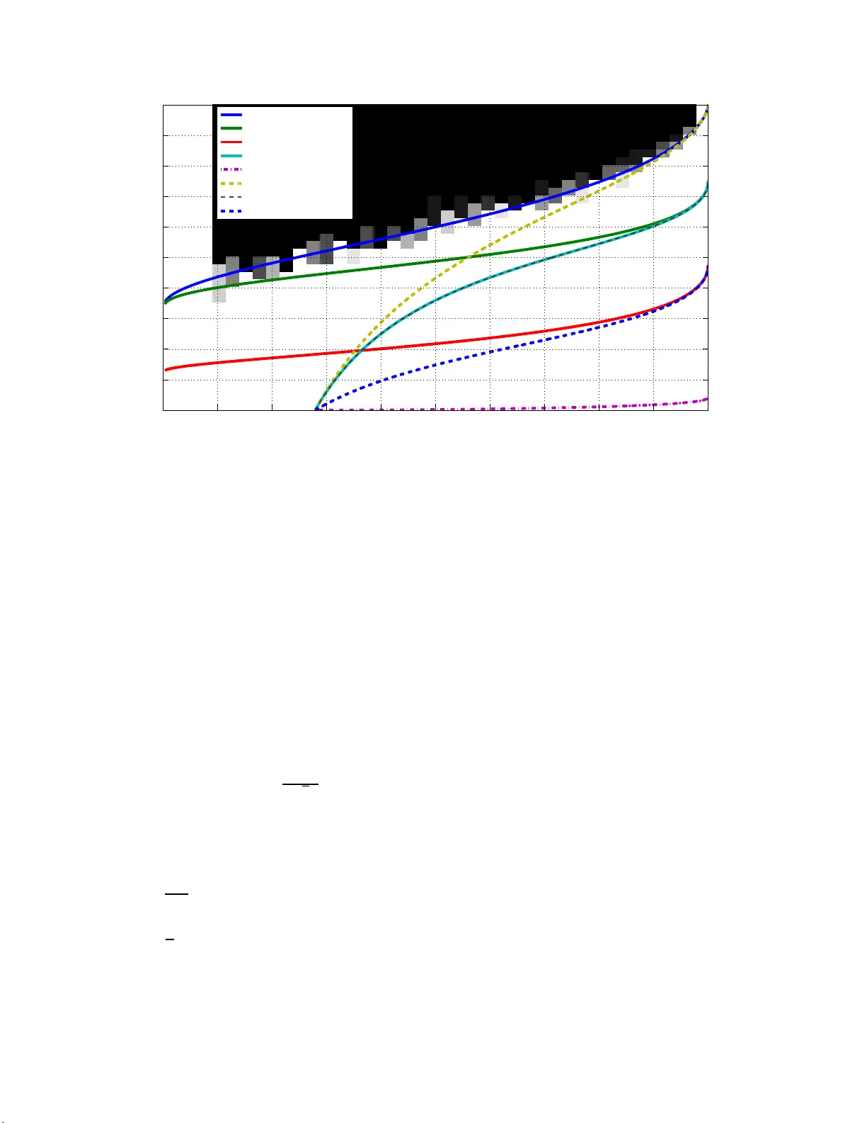
New Null Space Results and Reco v ery Thresholds for Matrix Rank Minimization Samet Oymak, Babak Hassibi California Institute of T ec hnology Email: { so ymak,hassibi } @caltec h.edu ∗ No v em b er 26, 2024 Abstract Nuclear norm minimization (NNM) has recent ly gained significant atten tion for its use in rank minimization problems. Similar to compresse d sensing, using null space c harac ter izations, re co very thresholds for NN M hav e been studied in [12, 4 ]. How ever sim ulations show that the thresholds are far from optimal, esp ecially in the low r ank region. In this pap er w e apply the recent analysis of Sto jnic for compressed sensing [18] to the n ull spa ce conditions of NNM. The resulting thr esholds are significantly b etter and in particula r our w eak threshold appears to match with simulation re sults. F urther our curves suggest for a n y r ank growing linearly with matrix size n we need only three times of ov ersa mpling (the mo del complexity) for weak recovery . Similar to [12] we analyze the conditions for weak, sectional and s trong thre sholds. Additionally a separate analysis is g iv en for special case of positive semidefinite matrices. W e conclude b y disc ussing simulation results and fut ure research directions. 1 In tro duction Rank minimizatio n (RM) addresses th e reco v ery of a lo w rank matrix from a set of linear measurements that pro j ect the matrix on to a lo w er dimen sional space. The p roblem has gained extensiv e atten tion in the past f ew yea rs, due to the promising applicabilit y in many practical problems [1]. Supp ose that X 0 is a low rank matrix of size n 1 × n 2 and let r ank( X ) = r . F urther let A : R n 1 × n 2 → R m b e a linear measuremen t op erator. Giv en the measurements y 0 = A ( X 0 ), the pr oblem is to reco v er X 0 , w ith the kno wledge of the fact that it is lo w rank. Pr o vided that X 0 is the solution with lo we st r ank, this problem can b e form ulated with the follo wing minimization program. min r ank( X ) (1) sub ject to A ( X ) = y 0 , The r an k ( · ) function is non-con v ex, and it turns out that (1) is NP hard and cannot b e solv ed effi- cien tly . F azel et a l. suggested replacing the rank w ith the n uclear norm heuristic as the cl osest co nv ex relaxation [1]. The resulting con ve x optimization program is called n uclear norm minimization and is as follo ws. min k X k ⋆ (2) sub ject to A ( X ) = A ( X 0 ) , ∗ This w ork w as su p ported in p art by the N ational Science F oundation und er gran ts CCF-07292 03, CNS-0932428 and CCF-10189 27, by the O ffice of N a v al Researc h under the MURI grant N00014-08-1-0747, and by Caltec h’s Lee Center for Adv anced Net w orking. 1 where k · k ⋆ refers to the n uclear norm of its argumen t, i.e., the su m of the singular v alues. (2) can b e written as a semi-definite program (SDP) and thus b e solv ed in p olynomial time. Recen t w orks h av e studied the sufficient conditions under which (2) will reco v er X 0 (i.e. X 0 is un iqu e m inimizer of (2)). In [3] it is sho wn that, similar to compressed sensing, Restricted Isometry Prop ert y (RIP ) is a sufficient condition for the su ccess of (2) and O ( r n 1 n 2 ( n 1 + n 2 ) log ( n 1 n 2 )) measurement is enough for gu aranteeing RIP w ith high p robabilit y . In [19], C andes extended th ese results and sh o wed that a minimal samp ling of O ( r n ) is in fact enough to h a ve RIP and hence reco very . In later w orks [4, 12], necessary and sufficien t n ull space conditions are derive d and w ere analyzed f or Ga uss ian measurement op erators, i.e., op erators where the en tries are i.i.d. Gauss ian, leading to thresholds for the su ccess of (2). These thresholds establish explicit relatio nsh ips b etw een the problem parameters, as o pp osed to the o rder -w ise relationships that result from RIP tec hniqu es. Ho w ev er these results are far from b eing optimal in the lo w rank regime whic h necessitate s a new approac h to b e tak en. In particula r, if the matrix size is n × n and the rank of the matrix to b e r eco v ered is β n then eve n if β > 0 is v ery small, they requ ir e a m inim um sampling of (1 − 64 9 π 2 ) n 2 for success. In th is pap er, w e co me up w ith a nov el null space analysis for the rank minimization problem and w e fin d significan tly b etter thresholds than t he results of [4, 1 2]. Although the analysis is nov el for the rank min imizat ion pr oblem, w e basically follo w the analysis dev elop ed for compressed sensing b y S to jnic in [18] wh ic h is based on a seminal result of Gordon [15]. In addition to the analysis of general matrices, we giv e a separate analysis for p ositiv e semid efinite matrices w h ic h resemble nonnegativ e vect ors in compressed s en sing. W e also consider the case of uniqu e p ositiv e semidefin ite solutions, whic h was recen tly analyzed by Xu in [23]. W e exte nsively u s e the r esults of [1 8]. Basically , we sligh tly mo dify Lemmas 2 , 5, 7 of [ 18] a nd use n ull space conditions for the NNM problem. The strength of this analysis comes from the facts that the analysis is more accessible and that the we ak threshold of [18] matc h es the exact threshold of [7]. In fact, while it is not at all clear ho w to extend the analysis of [7] from compressed sensing to N NM, it is relativ ely straight forward to do so for [18]. Our sim ulation results also indicate that our thresholds for the NNM p roblem are seemingly tigh t. This is p er h aps not s urprising since, as we shall see, the null space conditions for NNM and compressed sens ing are v ery similar. 2 Basic Definitions and Notations Denote identit y matrix of size n × n by I n . W e call U ∈ R m × n partial unitary if columns of U form an orthonormal set i.e. U T U = I n . Cle arly w e need n ≤ m for U to b e p artial u n itary . Also for a partial unitary U , let ¯ U denote an arbitrary partial unitary of size m × ( m − n ) so that [ U ¯ U ] is a un itary matrix (i.e. columns are complete orthonormal basis of R m ). F or a matrix X ∈ R m × n , w e denote the singular v alues by σ 1 ( X ) ≥ σ 2 ( X ) ≥ · · · ≥ σ q ( X ) where q = min( m, n ). The (skin n y) singular v alue d ecomp osition (SVD) of X is sho wn as X = U X Σ X V T X where U X ∈ R m × r , Σ X ∈ R r × r and V X ∈ R n × r , where r = rank( X ). Not e that U X , V X are partial unitary and Σ X is p ositiv e, d iag onal and full rank. Also let Σ( X ) denote ve ctor of increasingly ord ered singular v alues of X i.e. Σ( X ) = [ σ q ( X ) . . . σ 1 ( X )] T . The Ky-F an k n orm of X denoted b y k X k k is defined as k X k k = P k i =1 σ i ( X ). Wh en k = m in( m, n ) it is called the n uclear norm, i.e. k X k ⋆ , and when k = 1 it is equiv alen t to the s p ectral norm denoted by k X k . Also F rob enius n orm is denoted b y k X k F = p h X , X i = q P n i =1 σ 2 i ( X ) . Note that we alw a ys ha v e: k X k k = k X i =1 σ i ( X ) ≤ v u u t k X i =1 1 k X i =1 σ 2 i ( X ) ≤ √ k k X k F (3) F or a lin ear op erator A ( · ) acting on a linear sp ace, w e denote the n ull space of A by N ( A ), i.e. W ∈ N ( A ) iff A ( W ) = 0. W e d enote b y G ( d 1 , d 2 ) the ens em b le of real d 1 × d 2 matrices in whic h the en tries are i.i.d. N (0 , 1) (zero-mean, unit v ariance Gaussian). 2 It is a well kno wn fact that normalized singular v alues of a square matrix with i.i.d. Gaussian entries ha v e quarter circle distribu tion asymptotica lly [2]. In other w ords th e histogram of singular v alues (normalized b y 1 / √ n ) con v erges to the function φ ( x ) = √ 4 − x 2 π 0 ≤ x ≤ 2 (4) Similarly , the distribution of th e squares of th e singular v alues (normalized b y 1 /n ) con v erges to the wel l kno wn Marcenk o-P astur d istribution [2]. Note that this is n othin g bu t the distribution of the eigen v alues of X T X where X is a sq u are m atrix dr a wn from G ( n, n ), φ 2 ( x ) = √ 4 x − x 2 2 π x 0 ≤ x ≤ 4 (5) Let F ( x ) b e the cum ulativ e distrib ution f unction of φ ( x ) i.e., F ( x ) = Z x 0 φ ( t ) dt (6) Let 0 ≤ β ≤ 1. W e d efine γ ( β ) to b e the asymp totic normalized exp ected v alue of th e Ky-F an β n n orm of a matrix drawn f r om G ( n, n ), i.e.: γ ( β ) := lim n →∞ E [ k X k β n ] n 3 / 2 = Z 2 F − 1 (1 − β ) xφ ( x ) dx (7) Similarly define γ 2 ( β ) to b e the asymptotic normalized exp ected v alue of the Ky-F an β n norm of a matrix X T X where X is d r a w n from G ( n, n ): γ 2 ( β ) = lim n →∞ E  [ k X T X k β n ] n 2  = lim n →∞ E " P β n i =1 σ i ( X ) 2 n 2 # = Z 2 F − 1 (1 − β ) x 2 φ ( x ) dx (8) Note that these limits exist and γ ( β ) , γ 2 ( β ) is w ell defined [17]. A function f : R n → R is called L -Lipschitz if f or all x, y we ha v e: | f ( x ) − f ( y ) | ≤ L k x − y k ℓ 2 W e s a y an orthogonal pr o jection p air { P, Q } is a su pp ort of the matrix X if X = P X Q T . In particular { P X , Q X } is the uniqu e supp ort of the matrix X , if P X and Q X are orthogonal pro jectors with rank( P X ) = rank( Q X ) = rank( X ) suc h that X = P X X Q T X . In other w ords, P X = U X U T X and Q X = V X V T X . W e sa y A : R n 1 × n 2 → R m is a random Gaussian measuremen t op erator if the i th measuremen t is y i = A ( X ) i = trace( G T i X ) where { G i } m i =1 ’s a re i. i.d. matrices dra wn from G ( n 1 , n 2 ) for a ll 1 ≤ i ≤ m . Note that this is equiv alen t to y i = vec( G i ) T v ec( X ) wh ere v ec( X ) is obtained by putting column s of X on top of eac h other to get a v ector of size n 1 n 2 × 1. Mo del complexit y is defined as the n umb er of degrees of f r eedom of the matrix. F or a m atrix of size αn × n and rank αβ n mo del complexity is αβ (1 + α − αβ + o (1)) n 2 . Then we define normalized mo del complexit y to b e θ = β (1 + α − αβ ). Finally let  denote ”greater than” in partially ordered sets. In particular if A, B are Hermitian matrices then A  B ⇐ ⇒ A − B is p ositiv e semidefin ite. Similarly for a give n t wo v ectors u, v we write u  v ⇐ ⇒ u i ≥ v i ∀ i . 3 Key Lemmas to b e Used In this section, we state sev eral lemmas that we will mak e use of later. Pro ofs th at a re omitted can b e found in the giv en r eferen ces. F or Lemmas (1), (2), (3), let X, Y , Z ∈ R m × n with m ≤ n . 3 Lemma 1. tr ( X T Y ) ≤ m X i =1 σ i ( X ) σ i ( Y ) = Σ( X ) T Σ( Y ) (9) Pr o of. C an b e found in [20]. In c ase of ve ctors (i.e. matric es ar e diagonal) we have the fol lowing simple extension: L et x , y ∈ R m b e ve ctors. L et x [ i ] b e i ’th lar gest value of ve ctor | x | (i.e . | x | i = | x i | ) then h x , y i ≤ m X i =1 x [ i ] y [ i ] (10) Lemma 2. L et Z = X − Y . L et s i ( X, Y ) = | σ i ( X ) − σ i ( Y ) | and let s [1] ( X, Y ) ≥ s [2] ( X, Y ) ≥ · · · ≥ s [ m ] ( X, Y ) b e a de cr e asingly or der e d arr angement of { s i ( X, Y ) } m i =1 . Then we have the fol lowing ine quality: ∀ m ≥ k ≥ 1 : k X i =1 s [ i ] ( X, Y ) ≤ k X i =1 σ i ( Z ) = k Z k k (11) In p articular we have: m X i =1 | σ i ( X ) − σ i ( Y ) | ≤ k Z k ⋆ (12) Pr o of. Pr oof can b e found in [16, 21] Lemma 3. If matrix X =  X 11 X 12 X 21 X 22  then we have: k X k ⋆ ≥ k X 11 k ⋆ + k X 22 k ⋆ (13) Pr o of. Pr oof can b e found in [4]. Similarly, we have the fol lowing obvious ine quality when X is s quar e ( m = n ): k X k ⋆ ≥ tr ac e ( X ) (14) Pr o of. Dual n orm of th e n uclear norm is the sp ectral norm [16]. Remem b er that I m is identi ty . Then: k X k ⋆ = sup k Y k =1 h X, Y i ≥ h X , I m i = trace( X ) (15) Theorem 1. (Esc ap e th r ough a mesh, [15]) L et S b e a sub se t of the u nit Eu clide an spher e S n − 1 in R n . L et Y b e a r andom ( n − m ) -dimensional subsp ac e of R n , distribute d uniformly in t he G r assmanian with r esp e ct to Haar me asur e. L et ω ( S ) = E sup w ∈ S ( h T w ) (16) wher e h is a c olumn ve ctor dr awn fr om G ( n, 1) . Then if ω ( S ) < √ m − 1 4 √ m we have: P ( Y ∩ S = ∅ ) > 1 − 3 . 5 exp( −  √ m − 1 4 √ m − ω ( S )  2 18 (17) 4 Lemma 4. F or al l 1 ≤ k ≤ n , σ k ( X ) i s a 1 -Lipschitz function of X . Pr o of. Let X , ˆ X b e suc h that ˜ X = ˆ X − X and k ˜ X k F ≤ 1. But then from Lemma (2) w e ha ve : 1 ≥ k ˜ X k F ≥ σ 1 ( ˜ X ) ≥ s [1] ( X, ˆ X ) ≥ | σ k ( X ) − σ k ( ˆ X ) | (18) Lemma 5. (fr om [4, 13]) L et x b e dr awn fr om G ( n, 1) and f : R n → R b e a function with Lipschitz c onstant L then we have the fol lowing c onc entr ation ine quality P ( | f ( x ) − E f ( x ) | ≥ t ) ≤ 2 exp ( − t 2 2 L 2 ) (19) F or analyzing p ositiv e s emid efinite matrices, w e will introdu ce some more definitions and lemmas later on. 4 Thresholds for Square Matrices In the f ollo wing section, we’ll giv e and analyze strong, sectional and weak n ull space conditions for square matrices ( R n × n ). With minor mo difications, one can obtain the equiv alent results for rectangular matrices ( R αn × n ). 4.1 Strong Threshold Strong reco v ery thre shold. L et A : R n × n → R m b e a r andom Gaussian op er ator. We define β ( 0 ≤ β ≤ 1 ) to b e the str ong r e c overy thr e shol d if with high pr ob ability A satisfies the f ol lowing pr op erty: Any matrix X with r ank at most β n c an b e r e c over e d fr om me asur ements A ( X ) via (2). Lemma 6. Using (2) one c an r e c over al l matric es X of r ank at most r if and only if for al l W ∈ N ( A ) we have 2 k W k r < k W k ⋆ (20) Pr o of. If (20) holds then using Lemma (2) and the fact that σ i ( X ) = 0 ∀ i > r fo r any W we ha v e k X + W k ⋆ ≥ n X i =1 | σ i ( X ) − σ i ( W ) | ≥ r X i =1 ( σ i ( X ) − σ i ( W )) + n X i = r +1 σ i ( W ) (21) ≥ k X k ⋆ + k W k ⋆ − 2 k W k r > k X k ⋆ (22) Hence X is unique minimizer of (2). Con v ersely if (20) do esn’t hold for s ome W then c ho ose X = − W k where W k is the matrix induced b y setting all b ut largest r singular v alues of W to 0. Th en w e get: k X + W k = P n i = r +1 σ i ( W ) ≥ P r i =1 σ i ( W ) = P r i =1 σ i ( X ) = k X k ⋆ . Finally w e find rank( X ) ≤ r but X is not the unique minimizer. No w w e can sta rt analyzing the strong null space condition for the NNM problem. A is a random Gaussian operator and we’ ll analyze the linear regime wher e m = µn 2 and r = β n . Our aim is to determine the least µ (1 ≥ µ ≥ 0) so that β is a s tr ong thresh old for A . Similar to compressed sensing the n ull space of A is an n 2 − m dimensional random subspace of R n 2 distributed uniformly in the Grassmanian w.r.t. Haar measure. This can also b e viewed as the span of M = (1 − µ ) n 2 matrices { G i } M i =1 dra wn i.i.d. from G ( n, n ). Then similar to [18] w e ha ve established the necessary framewo rk. Let S s b e the set of all matrices su ch th at k W k ⋆ ≤ 2 k W k r and k W k F = 1. W e need to mak e sure the n ull space of A has no in tersection with S s . W e will first upp er b ound (16) in Theorem 1 then choose m (and µ ) resp ectiv ely . 5 As a first step, giv en a fixed H ∈ R n × n w e’ll calculate an upp er b ound on f ( H , S s ) = sup W ∈ S s v ec ( H ) T v ec ( W ) = sup W ∈ S s h H , W i . Note that fr om Lemm a 1 w e ha v e: f ( H, S s ) = s u p W ∈ S s h H , W i ≤ sup W ∈ S s Σ( H ) T Σ( W ) (23) The careful reader will notice that actuall y we ha v e equalit y in (23) b ecause the set S s is unitarily in v ariant hence an y v alue w e can get on the righ t han d side, we ca n also get on the left hand side b y aligning the singular v ectors of H and W . Let h = Σ( H ), w = Σ( W ). Note that h , w  0. Then since k w k ℓ 2 = k W k F = 1 and P n − r i =1 w i ≤ P n i = n − r +1 w i an y W ∈ S s , we need to solv e the follo w ing optimization problem giv en H : max y h T y (24) sub ject to y  0 n X i = n − r +1 y i ≥ n − r X i =1 y i k y k ℓ 2 ≤ 1 Clearly the righ t h and side of (23) and the result of (24) is same b ecause h T y will b e maximized when { y i } n i =1 are sorted increasingly du e to Lemm a 1. Note that (24) is exactly the same as (10) of [18]. Then w e can u se (22), (29) of [18] directly to get: Lemma 7. If h T z > 0 then f ( H, S s ) ≤ v u u t n X i = c +1 h 2 i − (( h T z ) − P c i =1 h i ) 2 n − c (25) wher e z ∈ R n such t hat z i = 1 ∀ 1 ≤ i ≤ n − r and z i = − 1 ∀ n − r + 1 ≤ i ≤ n and 0 ≤ c ≤ n − r such that ( h T z ) − P c i =1 h i ≥ ( n − c ) h c . As long as h T z > 0 we c an find such c ≥ 0 . In addition, in or der to minimize right hand side of (25), one should cho ose lar gest such c . In c ase of h T z ≤ 0 , the fol lowing is the obvious upp er b ound fr om Cauchy-Schwarz and t he fa ct th at k W k F = 1 f ( H, S s ) ≤ k h k ℓ 2 = v u u t n X i =1 h 2 i (26) Similar to [18], for the escap e through a mesh (ETM) analysis, using Lemma 7, we’ll consider the follo w ing wo rse u pp er b ound : Lemma 8. L et z b e define d same a s in L emma 7. L et H b e chosen fr om G ( n, n ) and let h = Σ( H ) and f ( H, S s ) = sup W ∈ S s h H , W i . Then we have: f ( H, S s ) ≤ B s wher e B s = k h k ℓ 2 if g ( H, c s ) ≤ 0 B s = v u u t n X i = c s +1 h 2 i − (( h T z ) − P c s i =1 h i ) 2 n − c s else wher e g ( H , c ) = ( h T z ) − P c i =1 h i n − c − h c and c s = δ s n is a c ≤ n − r such that c s = 0 if E [ h T z ] ≤ 0 c s is solution of (1 − ǫ ) E [( h T z ) − P c i =1 h i ] √ n ( n − c ) = F − 1  (1 + ǫ ) c n  else if E [ h T z ] > 0 (27) 6 wher e ǫ > 0 c an b e arbitr arily smal l. Note that c s is deterministic. Se c ond ly one c an observe that c s > 0 ⇐ ⇒ E [ h T z ] > 0 ⇐ ⇒ E [ h T z − P c s i =1 h i ] > 0 . Here F ( · ) is the c.d.f. of the quarter circle d istr ibution previously defined in (6). 4.1.1 Probabilistic Analysis of E [ B s ] The matrix H is dra wn from G ( n, n ) and E [ B s ] ≥ E [ f ( H , S s )]. In the f ollo wing discuss ion, we ’ll fo cus on the c ase E [ h T z ] > 0 and we ’ll declare failure (no reco very) el se. This is reasonable since our approac h will eve ntually lead to µ = 1 in case of E [ h T z ] ≤ 0. The reason is that, w ith high probab ility w e’ll ha v e g ( H, c s ) ≤ 0 and this will result in E [ B s ] ≈ E [ k H k F ] whic h is the worst upp er b ound. Then, we ’ll basically argue th at whenever E [ h T z ] > 0, asymptotica lly with p r obabilit y one, we’l l h a ve g ( H, c s ) > 0. Next, we ’ll show that contribution of the region g ( H , c s ) ≤ 0 to the exp ectatio n of B s asymptotically con verge s to 0. F rom the u nion b oun d, we ha v e: P ( g ( H, c s ) ≤ 0) ≤ P ( h T z − c s X i =1 h i ≤ (1 − ǫ ) E [( h T z ) − c s X i =1 h i ]) + P ( h c s ≥ √ nF − 1  (1 + ǫ ) c s n  ) (28) W e’ll analyze the tw o comp onen ts separately . Note that h T z − P c s i =1 h i is a fu nction of singular v alues whic h is actually a Lips c h itz f unction of the random matrix H as we’ll argue in the follo wing lemma. Lemma 9. L et H ∈ R n × n and let h = Σ ( H ) and z i s as define d pr eviously. Then: f ( H ) = h T z − c s X i =1 h i (29) is √ n − c s Lipschitz f unction of H . Pr o of. Let H , ˆ H , ˜ H b e suc h that ˜ H = H − ˆ H . F rom Lemma (2) we h a ve: k ˜ H k n − c s ≥ n − c s X i =1 | σ i ( H ) − σ i ( ˆ H ) | ≥ | r X i =1 ( σ i ( H ) − σ i ( ˆ H )) | + | n − c s X i = r +1 ( σ i ( ˆ H ) − σ i ( H )) | (30) ≥ | h T z − ˆ h T z | = | f ( H ) − f ( ˆ H ) | (31) On the other h and w e hav e: k ˜ H k n − c s ≤ √ n − c s k ˜ H k F whic h implies | f ( H ) − f ( ˆ H ) | ≤ √ n − c s k ˜ H k F finishing the pro of. No w, using the fact that H is i.i.d. Gaussian and h is the vec tor of singular v alues of H , w e ha v e E ( h T z − P c s i =1 h i ) = ( γ (1) − 2 γ ( β ) − ( γ (1) − γ (1 − δ s )) + o (1)) n 3 / 2 hence from L emm a 5 and from the fact that H is i.i.d. Ga ussian, w e hav e: P 1 := P ( h T z − c s X i =1 h i ≤ (1 − ǫ ) E [( h T z ) − c s X i =1 h i ]) ≤ exp( − ǫ 2 ( γ (1 − δ s ) − 2 γ ( β )) + o ( 1)) 2 n 2 2(1 − δ s ) ) (32) if E [ h T z ] > 0 (whic h is equiv alen t to E [ h T z − P c s i =1 h i ] > 0 and δ s > 0). Similarly f rom the qu arter circle law we ha v e E ( h c ) = ( F − 1 ( c/n ) + o (1)) √ n . Using Lemmas 5, 4 we can find : P 2 := P ( h c s ≥ √ nF − 1  (1 + ǫ ) c s n  ) ≤ exp( − n 2  F − 1  (1 + ǫ ) c s n  − F − 1  c s n  + o (1)  2 ) (33) 7 In particular w e alw a ys ha ve F − 1 ((1 + ǫ ) β ) − F − 1 ( β ) ≥ π ǫβ 2 for an y ǫ > 0, 1 > β ≥ 0 (b ecause F ( x ) ≤ 2 π for 0 ≤ x ≤ 2). Hence P 2 con v erges t o 0 exp onen tially fast. One can a ctually sho w P 2 ≤ exp( − O ( n 2 )) instead of exp( − O ( n )) ho we ver this w on’t affect the results. Then sin ce δ s > 0: P ( g ( H , c s ) ≤ 0) ≤ P 1 + P 2 ≤ exp( − n 8 ( π ǫδ s + o (1)) 2 ). It remains to u pp er b ound E ( B s ) as follo w s: E [ B s ] ≤ Z g ( H,c s ) ≤ 0 k h k ℓ 2 p ( H ) dH + Z H v u u t n X i = c s +1 h 2 i − (( h T z ) − P c s i =1 h i ) 2 n − c s p ( H ) dH (34) Note that g ( H, c ) is linear function of h (hence H ) so if g ( H , c ) ≤ 0 ⇐ ⇒ g ( aH , c ) ≤ 0 f or any a ≥ 0. In other words similar to the d iscussion in [18] for an y v alue of a = k H k F , the fr act ion of the region g ( H, c ) ≤ 0 on the sphere of r adius a will b e constan t. On the other hand since H is iid Gaussian, the pr ob ab ility distribution of H is ju st a function of k H k F i.e. p ( H = H 0 ) = f ( k H 0 k F ) = (2 π ) − n 2 / 2 exp( − 1 2 k H 0 k 2 F ) for an y matrix H 0 ∈ R n × n . As a result: Z g ( H,c s ) ≤ 0 , k H k F = a dH = C 0 Z | H k F = a dH = C 0 S a (35) where S a is the area of a sphere in R n × n with radius a . Hence P ( g ( H , c s ) ≤ 0) = Z a ≥ 0 Z g ( H,c s ) ≤ 0 , k H k F = a p ( H ) dH da = Z a ≥ 0 Z g ( H,c s ) ≤ 0 , k H k F = a f ( a ) dH da (36) = C 0 Z a ≥ 0 f ( a ) S a da = C 0 (37) Using the exact same argument: Z g ( H,c s ) ≤ 0 k H k F p ( H ) dH = Z ∞ a =0 Z g ( H,c s ) ≤ 0 , k H k F = a k H k F p ( H ) dH da = Z ∞ a =0 Z g ( H,c s ) ≤ 0 , k H k F = a af ( a ) dH da = Z ∞ a =0 af ( a ) C 0 S a = P ( g ( H , c s ) ≤ 0) E ( k H k F ) ≤ exp( − n 8 ( π ǫδ s + o (1)) 2 ) n (38) The last term clearly go es to zero for large n . Th en we need to calculate the second part which is: Z H v u u t n X i = c s +1 h 2 i − (( h T z ) − P c s i =1 h i ) 2 n − c s p ( H ) dH = E ( v u u t n X i = c s +1 h 2 i − (( h T z ) − P c s i =1 h i ) 2 n − c s ) (39) ≤ v u u t E ( n X i = c s +1 h 2 i − (( h T z ) − P c s i =1 h i ) 2 n − c s ) (40) The last inequalit y is d ue to the follo win g Cauc h y-Sc hw arz. F or a r andom v ariable (R.V.) X ≥ 0 E ( X ) = Z x xp ( x ) dx Z x p ( x ) dx ≥  Z x p xp ( x ) 2 dx  2 = E ( √ X ) 2 (41) Note that for large n and fixed c s = δ s n and r = β n we hav e E ( n X i = c s +1 h 2 i − (( h T z ) − P c s i =1 h i ) 2 n − c s ) =  γ 2 (1 − δ s ) − ( γ (1 − δ s ) − 2 γ ( β )) 2 1 − δ s + o (1)  n 2 (42) 8 Then com b ining (34) and (38), it follo ws that (42) give s an upp er b ou n d for E [ B s ] 2 and thereb y E [ f ( H, S s )] 2 . T o b e able to calculate the r equired num b er of measuremen ts we need to fi nd δ s and sub s titute in (42) b ecause (42) will also b e an upp er b ound on the m inim um m asymptotica lly . If w e consider (27), asymp totically δ s will b e solution of: (1 − ǫ ) γ (1 − δ s ) − 2 γ ( β ) 1 − δ s = F − 1 ((1 + ǫ ) δ s ) (4 3) Then w e can su b stitute this δ s in (42) to solv e for m (and µ ). Using T h eorem 1 an d (43) w e fin d: Theorem 2 . If γ (1) − 2 γ ( β ) ≤ 0 then µ = 1 . Otherwise: µ > γ 2 (1 − δ s ) − ( γ (1 − δ s ) − 2 γ ( β )) 2 1 − δ s (44) is sufficient sampling r ate for β to b e str ong thr eshold of r andom Gaussian op er ator A : R n × n → R µn 2 . Her e δ s is solution of: (1 − ǫ ) γ (1 − δ s ) − 2 γ ( β ) 1 − δ s = F − 1 ((1 + ǫ ) δ s ) (4 5) In order to get the smallest µ we let ǫ → 0. Nu merical calculations giv e the strong thr eshold in Figure 1. Obvio usly we found and plotted the least µ for a giv en β (i.e. equalit y in (44)). Next w e defin e and an alyze sectional threshold. 4.2 Sectional Threshold Sectional rec o very threshold. L e t A : R n × n → R m b e a r andom Gaussian op er ator and let { P , Q } b e an arbitr ary ortho gonal pr oje ction p air with r ank ( P ) = r ank ( Q ) = β n . Then we say that β ( 0 ≤ β ≤ 1 ) is a se ctional r e c overy thr eshold if w ith high pr ob ability A satisfies t he fol lowing pr op erty: Any matrix X with supp ort { P , Q } c an b e r e c over e d fr om m e asur ements A ( X ) via (2). Giv en a fixed β , our aim is to c alculate the least µ suc h that β is s ect ional threshold for a random Gaussian op erator A : R n × n → R µn 2 . Lemma 10. Given supp ort { P , Q } with r ank ( P ) = r ank ( Q ) = r one c an r e c over al l matric es X with this supp ort using (2) iff for al l W ∈ N ( A ) we have k ( I − P ) W ( I − Q T ) k ⋆ > k P W Q T k ⋆ (46) Pr o of. Note that in a suitable basis induced by { P , Q } we can write: X =  X 11 0 0 0  , W =  W 11 W 12 W 21 W 22  (47) where  W 11 0 0 0  = P W Q T ,  0 W 12 0 0  = P W ( I − Q T ) ,  0 0 W 21 0  = ( I − P ) W Q T ,  0 0 0 W 22  = ( I − P ) W ( I − Q T ). No w If (46) h olds then using Lemma 3 w e immediately ha ve for all W ∈ N ( A ): k X + W k ⋆ =  X 11 + W 11 W 12 W 21 W 22  ≥ k X 11 + W 11 k ⋆ + k W 22 k ⋆ ≥ k X 11 k ⋆ − k W 11 k ⋆ + k W 22 k ⋆ > k X 11 k ⋆ (48) Hence X is unique min imizer of (2). In [12], it wa s pro ve n that (4 6) is tight i n the s en se that if ther e exists W ∈ N ( A ) such that k ( I − P ) W ( I − Q T ) k ⋆ < k P W Q T k ⋆ then w e can find a n X with supp ort { P , Q } where X is not minim izer of (2 ). 9 No w we can start analyzing the sectional null space condition for the NNM problem. A is a random Gaussian op erator and w e’ll analyze the linear regime where m = µn 2 and r = β n . Similar to compr essed sensing, the n ull space of A is an n 2 − m dimensional r andom subsp ace of R n 2 distributed uniformly in the Grassmanian w.r.t. Haar measure. Then similar to [18] w e h a ve established the necessary framew ork. Let S sec b e the set of all matrices such that k ( I − P ) W ( I − Q T ) k ⋆ ≤ k P W Q T k ⋆ and k W k F = 1. W e need to mak e sure, the null s p ace has no inte rsection with S sec . W e will first upp er boun d (16) in Theorem 1, t hen c ho ose m (and µ ) resp ectiv ely . As d iscussed in [12], without loss of g eneralit y w e can assume X =  X 11 0 0 0  b ecause X can b e transformed to this form with a unitary transformation (whic h dep ends o nly on { P, Q } ) and since the null sp ace is uniformly c hosen (i.e. its basis is n 2 − m random matrices chosen iid from G ( n , n )) after this unitary transformation its distribution will still b e un iform. The reason is that if X is i.i.d. Gaussian matrix and A, B are fixed unitary matrices then AX B is still i.i.d. Gaussian. This further sho ws that th e pr obabilit y of successful reco very do es not dep end on { P, Q } as long a s β is fi xed. With this assumption S sec is the se t of all matrices with k W 22 k ⋆ ≤ k W 11 k ⋆ and k W k F = 1. Ob serv e that W 11 ∈ R r × r and W 22 ∈ R ( n − r ) × ( n − r ) . In the f ollo wing w e assume 2 × 2 blo c k m atrice s. Let X ij b e i ’th row and j ’th column blo c k of X . As a fi rst step, giv en a fixed H ∈ R n × n w e’ll calculate an upp er b ound on f ( H , S sec ) = sup W ∈ S sec v ec ( H ) T v ec ( W ) = sup W ∈ S sec h H , W i . Note that: h H , W i = P i,j h H ij , W ij i F urther let h 1 = Σ( H 11 ) , h 2 = Σ( H 22 ) , w 1 = Σ( W 11 ) , w 2 = Σ( W 22 ). Also le t h 3 b e in creasingly sorted absolute v alues of entries of submatrices H 12 , H 21 and w 3 is defined similarly . Finally let x i,j denote j ’th en try of ve ctor x i F rom Lemma 1 we h a ve: f ( H, S sec ) = sup W ∈ S sec h H , W i ≤ s up W ∈ S sec 3 X i =1 h T i w i (49) Similarly one can ac hiev e equalit y in inequalit y (49), although w e’ll not discuss h er e. On the other hand W ∈ S sec if and only if: k w 1 k ℓ 1 ≥ k w 2 k ℓ 1 (50) W e also ha v e k w 1 k 2 ℓ 2 + k w 2 k 2 ℓ 2 + k w 3 k 2 ℓ 2 = k W k 2 F = 1. Th en we need to solv e the follo wing optimization problem (remem b er that w i , h i  0 ∀ i ): max y 1 , y 2 , y 3 3 X i =1 h T i y i (51) sub ject to y i  0 ∀ i k y 1 k ℓ 1 ≥ k y 2 k ℓ 1 k y 1 k 2 ℓ 2 + k y 2 k 2 ℓ 2 + k y 3 k 2 ℓ 2 ≤ 1 Clearly , th e righ t h and side of (49) and result of (51) is same aga in due to Lemma 1 b ecause increasingly 10 sorting y i ’s will maximize the result. Now w e’ll rewrite (51) as follo ws: max y 1 , y 2 , y 3 a 1 + a 2 (52) sub ject to a 1 = h T 1 y 1 + h T 2 y 2 a 2 = h T 3 y 3 y i  0 ∀ i k y 1 k ℓ 1 ≥ k y 2 k ℓ 1 k y 1 k 2 ℓ 2 + k y 2 k 2 ℓ 2 ≤ E 1 k y 3 k 2 ℓ 2 ≤ E 2 E 1 + E 2 ≤ 1 No w, the question is reduced to solving the follo wing t wo optimiza tion p roblems and maximizing o ve r them b y app ropriately d istr ibuting E 1 , E 2 : max y 1 , y 2 h T 1 y 1 + h T 2 y 2 (53) sub ject to k y 1 k ℓ 1 ≥ k y 2 k ℓ 1 k y 1 k 2 ℓ 2 + k y 2 k 2 ℓ 2 ≤ 1 max y 3 h T 3 y 3 (54) sub ject to k y 3 k 2 ℓ 2 ≤ 1 Let resu lt of pr ogram (53) b e f 1 ( H , S sec ) and result of pr ogram (54) b e f 2 ( H , S sec ). Then clearly result of program (52) is max a 1 + a 2 (55) sub ject to a 1 = p E 1 f 1 ( H , S sec ) a 2 = p E 2 f 2 ( H , S sec ) E 1 + E 2 ≤ 1 It is clear that f 1 ( H , S sec ) , f 2 ( H , S sec ) ≥ 0. Then analyzi ng (55) w e get: f ( H, S sec ) ≤ a 1 + a 2 = p E 1 f 1 ( H , S sec ) + p E 2 f 2 ( H , S sec ) (56) ≤ p E 1 + E 2 p f 1 ( H , S sec ) 2 + f 2 ( H , S sec ) 2 ≤ p f 1 ( H , S sec ) 2 + f 2 ( H , S sec ) 2 Similarly one can also ac hiev e equalit y in (56) b y letting E 1 f 2 1 = E 2 f 2 2 . No w let u s turn to analyzing program (53). Luc kily [18] already give s the follo wing upp er b ound for this in equation (94). F or an y k h 1 k ℓ 1 ≤ k h 2 k ℓ 1 : f 1 ( H , S sec ) ≤ v u u t k h 1 k 2 ℓ 2 + k h 2 k 2 ℓ 2 − c X i =1 h 2 2 ,i − ( k h 2 k ℓ 1 − k h 1 k ℓ 1 − P c i =1 h 2 i ) 2 n − c (57) for an y c ≤ n − r su c h that k h 2 k ℓ 1 − k h 1 k ℓ 1 − P c i =1 h 2 ,i ≥ ( n − c ) h 2 ,c . 11 F or program (54) we ha ve: f 2 ( H , S sec ) ≤ h T 3 y 3 = h h 3 , y 3 i ≤ k h 3 k ℓ 2 k y 3 k ℓ 2 ≤ k h 3 k ℓ 2 (58) Com bining (56),(57),(58) w e find : f ( H, S sec ) ≤ v u u t k H k 2 F − c X i =1 h 2 2 ,i − ( k h 2 k ℓ 1 − k h 1 k ℓ 1 − P c i =1 h 2 ,i ) 2 n − c if k h 1 k ℓ 1 ≤ k h 2 k ℓ 1 (59) ≤ k H k F else (60) Using (59), for escap e thr ough a mesh (ETM) an alysis we’ll u se the follo wing u pp er b ounding tec h- nique: Lemma 11. L et H b e chosen fr om G ( n, n ) and let h 1 = Σ( H 11 ) and h 2 = Σ( H 22 ) . f ( H , S sec ) = sup W ∈ S sec h H , W i . Then we have: f ( H, S sec ) ≤ B sec wher e B sec = k H k F if g ( H, c sec ) ≤ 0 B sec = v u u t k H k 2 F − c sec X i =1 h 2 2 ,i − ( k h 2 k ℓ 1 − k h 1 k ℓ 1 − P c sec i =1 h 2 ,i ) 2 n − c sec else wher e g ( H , c ) = k h 2 k ℓ 1 −k h 1 k ℓ 1 − P c i =1 h 2 ,i n − c − h 2 ,c and c sec = δ sec n (1 − β ) is a c ≤ n (1 − β ) such that c sec = 0 if E [ k h 2 k ℓ 1 ] ≤ E [ k h 1 k ℓ 1 ] c sec is solution of (1 − ǫ ) E [( k h 2 k ℓ 1 − k h 1 k ℓ 1 ) − P c i =1 h 2 ,i ] p n (1 − β )( n − c ) = F − 1  (1 + ǫ ) c n (1 − β )  else E [ k h 2 k ℓ 1 ] > E [ k h 1 k ℓ 1 ] (61) wher e ǫ > 0 c an b e arbitr arily smal l. 4.2.1 Probabilistic Analysis of E [ B sec ] In order to do the ETM analysis, w e c ho ose H from G ( n, n ). Clearly E [ B sec ] ≥ E [ f ( H, S sec )] hence we need to find an upp er b ound on E [ B sec ]. Similar to probabilistic analysis of strong thresh old, we’ll s ho w that with high p r obabilit y g ( H , c sec ) > 0 w h enev er E [ k h 2 k ℓ 1 − k h 1 k ℓ 1 ] > 0. W e’ll declare failure else. (F ailure implies µ = 1). Note that when E [ k h 2 k ℓ 1 − k h 1 k ℓ 1 ] > 0, we ha v e c sec > 0. P ( g ( H, c sec ) ≤ 0) ≤ P 1 + P 2 where (62) P 1 = P ( h 2 ,c sec ≥ p n (1 − β ) F − 1  (1 + ǫ ) c sec n (1 − β )  ) (63) P 2 = P ( k h 2 k ℓ 1 − k h 1 k ℓ 1 − c sec X i =1 h 2 ,i ≤ (1 − ǫ ) E [ k h 2 k ℓ 1 − k h 1 k ℓ 1 − c sec X i =1 h 2 ,i ]) (64) Remem b er that h 2 ,i is i ’th smallest singular v alue of the submatrix H 22 whic h is dra wn from G ( n (1 − β ) , n (1 − β )). F rom quarter circle d istribution it f ollo ws: E [ h 2 ,c sec ] = p n (1 − β )( F − 1 ( δ sec ) + o (1)) (65) Then similar to the analysis of the strong r eco ve ry u s ing Lemm as 4, 5 and the fact that H is iid Gaussian, w e fin d P 1 ≤ exp  − n (1 − β ) 8 ( π ǫδ sec + o (1)) 2  (66) No w we ’ll analyze P 2 using Lipsc hitzness. 12 Lemma 12 . L et f ( H ) = k h 2 k ℓ 1 − k h 1 k ℓ 1 − P c sec i =1 h 2 ,i . Then f is √ n − c sec Lipschitz function of H . Pr o of. Assu me w e ha v e 2 × 2 blo c k matrices ˜ H = ˆ H − H ∈ R n × n with up p er left blo c k ha ving size r × r . Also let k ˜ H k F = 1. Th en w e ha v e 1 ≥ k ˜ H 11 k 2 F + k ˜ H 22 k 2 F ≥ r X i =1 σ i ( ˜ H 11 ) 2 + n − r − c sec X i =1 σ i ( ˜ H 22 ) 2 (67) = ⇒ √ n − c sec ≥ r X i =1 σ i ( ˜ H 11 ) + n − r − c sec X i =1 σ i ( ˜ H 22 ) (68) No w using Lemma 2 we get: k ˜ H 11 k r + k ˜ H 22 k n − r − c sec ≥ r X i =1 | σ i ( ˆ H 11 ) − σ i ( H 11 ) | + n − r − c sec X i =1 | σ i ( ˆ H 22 ) − σ i ( H 22 ) | (69) ≥ | f ( H ) − f ( ˆ H ) | (70) Com bining all we fi nd: √ n − c sec ≥ | f ( H ) − f ( ˆ H ) | as d esired. Note that asymptotically E [ f ( H )] = ((1 − β ) 3 / 2 γ (1 − δ s ) − β 3 / 2 γ (1) + o (1)) n 3 / 2 b ecause h 1 , h 2 are v ectors of singular v alues of H 11 and H 22 resp ectiv ely . F r om (12) and (5) w e find P 2 ≤ exp  − n 2 ǫ 2 2(1 − δ s (1 − β )) ((1 − β ) 3 / 2 γ (1 − δ s ) − β 3 / 2 γ (1) + o (1)) 2  (71) Finally we sho w ed P ( g ( H , c sec ) ≤ 0) ≤ P 1 + P 2 deca ys t o 0 exponentiall y fast as n → ∞ . T hen we use the follo wing up p er b ound for E [ B sec ]: E [ B sec ] ≤ Z g ( H,c s ) ≤ 0 k H k F p ( H ) dH + Z H v u u t k H k F − c sec X i =1 h 2 2 ,i − ( k h 2 k ℓ 1 − k h 1 k ℓ 1 − P c sec i =1 h 2 ,i ) 2 n − c sec p ( H ) dH (72) Using exactly same argumen ts in [18] and (38) w e ha ve : Z g ( H,c s ) ≤ 0 k H k F p ( H ) dH ≤ exp( − n (1 − β ) 8 ( π ǫδ s + o (1)) 2 ) n → 0 (73) as n → ∞ . Secondly using p E [ X ] ≥ E [ √ X ] for an y R.V. X ≥ 0 we hav e: E   v u u t k H k F − c sec X i =1 h 2 2 ,i − ( k h 2 k ℓ 1 − k h 1 k ℓ 1 − P c sec i =1 h 2 ,i ) 2 n − c sec   (74) ≤ n s 1 − (1 − β ) 2 (1 − γ 2 (1 − δ sec )) − ((1 − β ) 3 / 2 γ (1 − δ sec ) − β 3 / 2 γ (1)) 2 1 − δ sec (1 − β ) + o (1) (75) Com bining (73), (74) w e find that asymptotically the right hand side of (7 4) is an upp er b ound for E [ B sec ]. Using this we can conclud e: Theorem 3 . If β ≥ 1 2 then µ = 1 . Otherwise: µ > 1 − (1 − β ) 2 (1 − γ 2 (1 − δ sec )) − ((1 − β ) 3 / 2 γ (1 − δ sec ) − β 3 / 2 γ (1)) 2 1 − δ sec (1 − β ) (76) 13 is a sufficient sampling r ate f or β to b e se ctional thr eshold of Gaussian op er ator A : R n × n → R µn 2 , wher e 0 < δ sec < 1 is solution of (fr om (6 1)) (1 − ǫ ) (1 − β ) 3 / 2 γ (1 − δ ) − β 3 / 2 γ (1) √ 1 − β (1 − δ (1 − β )) = F − 1 ((1 + ǫ ) δ ) (77) In order to find the least µ w e let ǫ → 0. Numerical calculations r esu lt in sectional threshold of Figure (1). 4.3 W eak Threshold In this section, we’ ll d eriv e the relation b et w een µ and β for the w eak th reshold d escrib ed b elow. W eak reco very threshold. L et A : R n × n → R m b e a r andom Gaussia n o p er ator and let X ∈ R n × n b e an arbitr ary matrix with r ank ( X ) = β n . We say that β is a we ak r e c overy thr eshold if with high pr ob ability this p articular matrix X c an b e r e c over e d fr om m e asur ements A ( X ) via pr o gr am (2). W e remark that the w eak threshold is the one that c an b e observ ed from simulat ions. The strong (and sectio nal) thr esh olds cannot b ecause there is no wa y to c hec k the reco very of all lo w rank X (o r all X of a particular su p p ort). In this sense, th e weak th reshold is the most imp ortan t. Again giv en a fixed β , we’ll aim to the least µ su c h that β is w eak thresh old for a r andom Gaussian op erator A : R n × n → R µn 2 . In order to preven t rep etitions, we’l l b e more concise in this section b ecause man y of the d eriv ations are rep etitions of the deriv ations for strong an d sectional thresholds. Lemma 13. L et X ∈ R n × n with r ank ( X ) = r , SVD X = U Σ V T with Σ ∈ R r × r . Then it c an b e r e c over e d using (2) iff for al l W ∈ N ( A ) we have tr ac e ( U T W V ) + k ¯ U T W ¯ V k ⋆ > 0 (78) wher e ¯ U , ¯ V such that [ U ¯ U ] and [ V ¯ V ] ar e unitar y. Pr o of. S ince sin gu lar v alues are unitarily inv ariant , if (78) holds usin g Lemma (3): k X + W k ⋆ = k [ U ¯ U ] T ( X + W )[ V ¯ V ] k ⋆ =      Σ 0 0 0  +  U T W V . . . . . . ¯ U T W ¯ V      ⋆ (79) ≥ k Σ + U T W V k ⋆ + k ¯ U T W ¯ V k ⋆ ≥ trace(Σ + U T W V ) + k ¯ U T W ¯ V k ⋆ (80) ≥ k X k ⋆ + trace( U T W V ) + k ¯ U T W ¯ V k ⋆ > k X k ⋆ (81) Hence X is uniqu e minimizer of p rogram (2). In [1 2], it wa s sho wn that co nd itio n (78) is tig ht in th e sense that if there is a W ∈ N ( A ) su c h that trace( U T W V ) + k ¯ U T W ¯ V k ⋆ < 0 then X is not minimizer of (2). Note t hat c onditions (78) is indep endent of singular va lues of X . This suggests that no t only X but also al l matric es with same left and right singular ve ctors U, V ar e r e c over able via (2). Analyzing the condition: A is a random Gaussian op erator and w e’ll analyz e th e linear regime where m = µn 2 and r = β n with β > 0. Let S w b e the set of all matrices suc h that trace( U T W V ) + k ¯ U T W ¯ V k ⋆ ≤ 0 and k W k F = 1. W e need to make su re null space N ( A ) has no intersect ion with S w . W e first upp er b ound (16) in Theorem 1, then choose m (and µ ) r esp ectiv ely . As discussed in [12], without loss of generalit y we ca n assum e X =  Σ 0 0 0  where Σ ∈ R r × r is diag onal matrix with p ositiv e diago nal. This is b ecause any X = U Σ V T can b e transform ed into this form b y unitary transformation [ U ¯ U ] T X [ V ¯ V ] and since n ull space is uniformly c hosen (i.e. its basis is n 2 − m random matrices iid chosen from G ( n, n )) after unitary 14 transformation its distribution will still b e u niform. T h en S w can b e assumed to b e set of matrices with trace( W 11 ) + k W 22 k ⋆ ≤ 0 and k W k F = 1. Again we assume 2 × 2 blo c k matrices. Firstly , giv en a fixed H ∈ R n × n w e’ll calculate an u pp er b ound on f ( H, S w ) = sup W ∈ S w h H , W i . Let h 1 = diag ( H 11 ) i.e. diagonal entrie s of H 11 , h 2 = Σ( H 22 ) and let h 3 b e increasingly sorted absolute v alues o f remaining entries, which are en tries of H 12 , H 21 and off-diagonal entries of H 11 . w 1 , w 2 , w 3 is defined similarly . Also let x i,j denote j ’th en try of ve ctor x i . F rom Lemma (1) we ha v e: f ( H, S w ) = sup W ∈ S w h H , W i ≤ sup W ∈ S w 3 X i =1 h T i w i (82) W e in tro duce the follo wing notatio n. Let s ( x ) denote summation o f en tries of x i.e. s ( x ) = P i x i . Then W ∈ S w if and only if: s ( w 1 ) + k w 2 k ℓ 1 ≤ 0 and (83) k w 1 k 2 ℓ 2 + k w 2 k 2 ℓ 2 + k w 3 k 2 ℓ 2 = k W k 2 F = 1 (84) Then we need to solv e the follo wing equiv alen t optimizatio n p roblem giv en H (Note that w i , h i  0 ∀ 2 ≤ i ≤ 3): max y 1 , y 2 , y 3 3 X i =1 h T i y i (85) sub ject to y 2 , y 3  0 s ( y 1 ) + k y 2 k ℓ 1 ≤ 0 k y 1 k 2 ℓ 2 + k y 2 k 2 ℓ 2 + k y 3 k 2 ℓ 2 ≤ 1 Righ t hand sid e of (82) and outp u t of (85) is same. W e’ll rewr ite (85) as follo ws: max y 1 , y 2 , y 3 a 1 + a 2 (86) sub ject to a 1 = h T 1 y 1 + h T 2 y 2 a 2 = h T 3 y 3 y 2 , y 3  0 s ( y 1 ) + k y 2 k ℓ 1 ≤ 0 k y 1 k 2 ℓ 2 + k y 2 k 2 ℓ 2 ≤ E 1 k y 3 k 2 ℓ 2 ≤ E 2 E 1 + E 2 ≤ 1 Note that (8 6) is essen tially sa me a s (6 7) of [18]. Basically ( 86) has add itional terms of h 3 , y 3 and y 1 ,i corresp onds − y n − r + i of [18] for 1 ≤ i ≤ r and y 2 ,j corresp onds y j of [18] for 1 ≤ j ≤ n − r . Th en rep eati ng exactly same steps that come b efore Lemma (11) and equation (59) and using (67 ), (68) of [18] we find: Lemma 14 . f ( H, S w ) ≤ v u u t k H k 2 F − c X i =1 h 2 2 ,i − ( k h 2 k ℓ 1 + s ( h 1 ) − P c i =1 h 2 ,i ) 2 n − c if s ( h 1 ) + k h 2 k ℓ 1 > 0 (87) ≤ k H k F else (88) for any 0 ≤ c ≤ n − r such that s ( h 1 ) + k h 2 k ℓ 1 − P c i =1 h 2 ,i ≥ ( n − c ) h 2 ,c . 15 Based on Lemma 14, for ETM analysis we’ll use the follo w in g lemma: Lemma 15. L et H b e chosen fr om G ( n, n ) and let h 1 = diag ( H 11 ) , h 2 = Σ( H 22 ) and f ( H, S w ) = sup W ∈ S w h H , W i . Then we have: f ( H, S w ) ≤ B w wher e B w = k H k F if g ( H , c w ) ≤ 0 B w = v u u t k H k 2 F − c w X i =1 h 2 2 ,i − ( k h 2 k ℓ 1 + s ( h 1 ) − P c w i =1 h 2 ,i ) 2 n − c w else wher e g ( H , c ) = k h 2 k ℓ 1 + s ( h 1 ) − P c i =1 h 2 ,i n − c − h 2 ,c and c w = δ w n (1 − β ) is a c ≤ n (1 − β ) such that c w = 0 if E [ k h 2 k ℓ 1 + s ( h 1 )] ≤ 0 c w is solution of (1 − ǫ ) E [ k h 2 k ℓ 1 + s ( h 1 ) − P c i =1 h 2 ,i ] p n (1 − β )( n − c ) = F − 1  (1 + ǫ ) c n (1 − β )  else E [ k h 2 k ℓ 1 + s ( h 1 )] > 0 (89) wher e ǫ > 0 c an b e arbitr arily smal l. Note that, when H is iid Gaussian, f or an y β < 1 we h a ve E [ k h 2 k ℓ 1 + s ( h 1 )] > 0 since en tries of h 1 is iid Gaussian hence E [ s ( h 1 )] = 0 an d clearly E [ k h 2 k ℓ 1 ] > 0. As a r esult c w > 0 to o. 4.3.1 Probabilistic Analysis of E [ B w ] Similar to previous analysis H is drawn from G ( n, n ) and in ord er to u se T h eorem 1 we need to upp er b ound E [ B w ]. Using the same steps and letting f ( H ) = k h 2 k ℓ 1 + s ( h 1 ) − P c w i =1 h 2 ,i : P ( g ( H, c w ) ≤ 0) ≤ P 1 + P 2 where (90) P 1 = P ( h 2 ,c w ≥ p n (1 − β ) F − 1  (1 + ǫ ) c w n (1 − β )  ) (91) P 2 = P ( f ( H ) ≤ (1 − ǫ ) E [ f ( H )]) (92) An up p er b oun d for P 1 w as already giv en in (66). Also similar to Lemma (12) one ca n sho w f ( H ) is √ n − c w Lipsc hitz function o f H . Therefore g ( H , c w ) w ill approac h to 0 exp onen tially fast ( e − O ( n ) ). Com bining this and the same argumen ts prior to (74) yields: E [ B w ] ≤ v u u t E " k H k 2 F − c w X i =1 h 2 2 ,i − ( k h 2 k ℓ 1 + s ( h 1 ) − P c w i =1 h 2 ,i ) 2 n − c w # + o (1) (93 ) ≤ n s 1 − (1 − β ) 2 (1 − γ 2 (1 − δ w )) − (1 − β ) 3 γ (1 − δ w ) 2 1 − δ w (1 − β ) + o (1) (94) Then using Theorem 1 and (89) we can wr ite: Theorem 4 . µ > 1 − (1 − β ) 2 (1 − γ 2 (1 − δ w )) − (1 − β ) 3 γ (1 − δ w ) 2 1 − δ w (1 − β ) (95) is a sufficient sampling r ate for β to b e we ak thr eshold of Gaussian op er ator A : R n × n → R µn 2 wher e 0 < δ w < 1 is solution of (1 − ǫ ) (1 − β ) 3 / 2 γ (1 − δ ) √ 1 − β (1 − δ (1 − β )) = F − 1 ((1 + ǫ ) δ ) (96) T o fin d the least µ we let ǫ → 0. Numerical calculations r esult in w eak threshold of Figure (1). 16 µ (Required Sampling) θ / µ (Oversampling −1 ) 0 0.1 0.2 0.3 0.4 0.5 0.6 0.7 0.8 0.9 1 0 0.1 0.2 0.3 0.4 0.5 0.6 0.7 0.8 0.9 1 Weak threshold Sectional threhold Strong threshold Weak thresh of [4] Strong thresh of [4] Weak thresh of [12] Sectional thresh of [12] Strong thresh of [12] Figure 1: Results of [4, 12] vs results w e get b y using escape through a mesh (ETM) analysis similar to [18] (F or square matrices). Here θ is model complexit y i .e. degrees of fr eedom of the matri x, ( θ = β (2 − β )). This plot gives the efficiency of nuclea r norm minimization as a function of num ber of samples µ . It gives at a certain µ , how muc h more one should ov ersample the con ten t of the matrix to p erform NNM succ essfull y . Simulations are done for 40 × 40 matrices and program ( 2) is solved with Gaussian measuremen ts. Our we ak threshold and simulations m atc h almost exact ly . Blac k regions indicate failure and white regions mean succe ss. Due to low precision (40 i s small ), we did not include simulat ion results for µ ≤ 0 . 1. 5 Thresholds for P ositiv e Semidefinite Matrices 5.1 Additional Not ations and Lemm as Before starting our analysis, we’ll briefly in tro duce some more notations and lemmas. S n denotes the set of Hermitian (real and symm etric) matrices of size n × n . Similarly S n + denotes the set of p ositiv e semidefinite matrices. PSD stands for p ositiv e semidefinite. Let N s ( A ) ⊂ N ( A ) d enote subspace of n ull space of A which consists of Hermitian matrices. Denote Gaussian unitary ensemble b y D ( n ) wh ich is e nsemble of Hermitian matrices of size n × n with ind ep end en t Gaussian en tries in th e lo wer tr iangular part, where off-diagonal en tries h a ve v ariance 1 and diag onal en tries hav e v ariance 2. In ord er to create suc h a matrix B one can c h oose a matrix A from G ( n , n ) and then let B = A + A T √ 2 . Let X ∈ S n with rank( X ) = r . T hen (skinny) eigen v alue deco mp osition (EVD) of X is X = U Λ U T for some partial unitary U ∈ R n × r and d iag onal matrix Λ ∈ R r × r . Denote i ’th largest eigen v alue of X b y λ i ( X ) for 1 ≤ i ≤ n . Let Λ( X ) denote increa singly ordered eigen v alues of X ∈ S n i.e. Λ( X ) = [ λ n ( X ) . . . λ 1 ( X )]. Also note that singular v alues of X corresp ond s to absolute v alues of eigen v alues of X . Let c = p 1 / 2. If A ∈ S n is a symmetric real matrix, defin e v ec ( A ) ∈ R n ( n +1) / 2 to b e follo wing vec tor: v ec ( A ) = 1 c [ cA 1 , 1 A 2 , 1 . . . A n, 1 cA 2 , 2 A 3 , 2 . . . A n, 2 cA 3 , 3 A 3 , 4 . . . cA n − 1 ,n − 1 A n,n − 1 cA nn ] T (97) In other w ords for eac h i w e let b i = [ cA i,i A i +1 ,i . . . A n,i ] /c and we let v ec ( A ) = [ b 1 b 2 . . . b n ] T . No w note that for any A, B ∈ S n w e hav e h A, B i = X i,j A i,j B i,j = X i A i,i B i,i + 2 X i 0 or (118) η − ( ¯ U T W ¯ U ) > 0 (119) where [ U ¯ U ] is a un itary matrix. 19 Pr o of. If W is not hermitian th en X + W is not herm itia n thus not PS D. If trace( W ) > 0 then trace( X + W ) > trace( X ) as desired. O n the other h an d if ¯ U T W ¯ U has a negativ e eigen v alue, we can w r ite Y := [ U ¯ U ] T ( X + W )[ U ¯ U ] =  Λ + U T W U . . . . . . ¯ U T W ¯ U  (120) whic h means low er right sub matrix ¯ U T W ¯ U of Y (whic h is a principal submatrix) is not PS D. Then it immediately f ollo ws that Y is n ot PSD, b ecause we can fin d a v ector v ∈ R n to m ak e v T Y v < 0. Then X + W is not PS D as it can b e obtained by unitarily transform in g Y (i.e. [ U ¯ U ] Y [ U ¯ U ] T ) wh ic h preserve s eigen v alues. Then as long as W satisfies one of the (117), X + W cannot b e minimizer hence X is unique minimizer. One can also giv e the if and only if condition for PSD weak reco v ery . Without pr oof, we’ll state the difference from Lemma 20: F or all W ∈ N ( A ) w e should h a ve: (117) or (118 ) or (119) or ”column space of ¯ U T W U is not a subset o f column space of ¯ U T W ¯ U ” . Ho w ev er, this last cond ition (in b old) wo uld not hav e any affect in our ETM analysis. (Agai n w ithout pro of ) The reason is t hat, with arbitrarily small p erturbation w e can m ak e ¯ U T W ¯ U full rank, while not c hanging other pr op erties of W at all, hence the last condition w ill b e obsolete. Lemma 21. Conditions (117, 118, 119) is also suffic i ent to guar ante e se ctional r e c overy. In other wor ds given an X = U Λ U T , if (117, 118, 119) holds for al l W ∈ N ( A ) , then in addition to r e c over ability of X , we c an r e c over a l l PSD matric es Y with supp ort { U U T , U U T } fr om me asur ements A ( Y ) with (113). Pr o of. Any PSD Y with sup p ort U U T can b e w r itten as Y = U Y Λ Y U T Y with U Y U T Y = U U T . Now, assume (117, 118, 119) holds. Then, if w e hav e η − ( ¯ U T Y W ¯ U Y ) > 0 whenev er η − ( ¯ U T W ¯ U ) > 0, usin g Lemma (20) w e are done, b ecause all conditions f or Y b ecome satisfied. As a result, it remains to show: η − ( ¯ U T Y W ¯ U Y ) > 0 ⇐ ⇒ η − ( ¯ U T W ¯ U ) > 0 Pr o of. Let v ∈ R n − r suc h that v T ¯ U T W ¯ U v < 0. Then since column spaces of ¯ U and ¯ U Y are same w e can c ho ose v 2 = ¯ U T Y ¯ U v so that ¯ U Y v 2 = ¯ U v = ⇒ v T 2 ¯ U T Y W ¯ U Y v 2 < 0. This result suggests that there is n o n eed to an alyze sectional condition separately b ecause results w e get for we ak will also work for sectional. No w we’ll start null space analysis. Let A : R n × n → R m b e random Gaussian op erator where m = µn ( n + 1) / 2 (0 ≤ µ ≤ 1). In [23] it w as argu ed that d istribution of N s ( A ) (n ull space r estricte d to hermitians) is equiv alen t to a subs p ace h a vin g matrices { D i } n ( n +1) / 2 − m i =1 as basis where { D i } n ( n +1) / 2 − m i =1 is dr a wn iid from D ( n ). This is easy to see when w e consider A ( · ) as a mapping f r om low er triangular en tries to R m . This also implies distribu tion of N s ( A ) is unitarily inv arian t b ecause if D is c hosen from D ( n ) then for a fixed unitary matrix V , V D V T and D has same distribution (ident ical random v ariables). Pr o of. D is equiv alen t to ( G + G T ) / √ 2 w h ere G is c hosen from G ( n , n ). Th en V DV T is e quiv alen t to ( V GV T + ( V GV T ) T ) / √ 2. No w using distribution of V GV T is equiv alen t to t hat o f G w e e nd up with the desired result. Let X = U Λ U T b e give n where rank( X ) = r = β n . Similar to previous analysis let S w p denote the set of herm itian matrice s W so that trace( W ) ≤ 0, η − ( ¯ U T W ¯ U ) = 0 and k W k F = 1. Since N s ( A ) is unitarily in v ariant w e can assume X is d iagonal and: X =  Λ 0 0 0  . No w cond itio n η − ( ¯ U T W ¯ U ) = 0 can 20 b e r eplace d by η − ( W 22 ) = 0. W e w an t to mak e sur e that N s ( A ) do es not int ersect with S w p so that null space condition (117) will b e satisfied. Note that this can b e rewr itten in th e follo win g wa y w hic h will enable us to us e Theorem 1. Let v ec ( N s ( A )) b e the subspace formed b y applying v ec ( . ) to elemen ts of N s ( A ). Then its distrib u tion is equiv alen t to a su bspace in R n ( n +1) / 2 ha ving basis { d i } (1 − µ ) n ( n +1) / 2 i =1 where { d i } i ’s are iid vec tors dra w n from G ( n ( n + 1) / 2 , 1). This is b ecause rand om v ectors { v ec ( D i ) } i are equiv alent to { d i } i scaled by √ 2. Similarly let v ec ( S w p ) b e the set of v ectors obtained by applying v ec ( . ) to elemen ts of S w p . Then b ecause vec ( . ) is linear, N s ( A ) ∩ S w p = ∅ ⇐ ⇒ v ec ( N s ( A )) ∩ v ec ( S w p ) = ∅ . Let h b e dra wn from G ( n ( n + 1) / 2 , 1) an d let D b e dr a w n from D ( n ). Since vec ( . ) also preserv es in n er pro du cts, in order to use Theorem (1) as previously we j u st need to calc ulate: ω ( S w p ) = E [ sup w ∈ v ec ( S wp ) h T w ] = 1 √ 2 E [ sup W ∈ S wp h D , W i ] (121) Let H b e Hermitian and defi n e f ( H , S w p ) = sup W ∈ S wp h H , W i . Then we’ll firstly upp er b ound f ( H, S sw ) then tak e exp ectation of up p er b ound as previously . Let s ( x ) denote sum matio n of entries of v ector x . Let h 1 denote the d iago nal entries of H 11 , h 2 = Λ( H 2 , 2 ) and h 3 denote increasingly ordered absoute v alues of entries of H 12 , H 21 and off-diagonal en tries of H 11 . w 1 , w 2 , w 3 are defin ed similarly for W . Note that W ∈ S sw if and only if w 2  0 (i.e. W 2 , 2 PSD) (122) s ( w 1 ) + s ( w 2 ) ≤ 0 (123) k w 1 k 2 ℓ 2 + k w 2 k 2 ℓ 2 + k w 3 k 2 ℓ 2 = 1 (1 24) No w using Lemma (1) we write: h H , W i ≤ h T 1 w 1 + h T 3 w 3 + h H 22 , W 22 i (125) Let H 2 , 2 = H + 2 , 2 − H − 2 , 2 where b oth of H + 2 , 2 , H − 2 , 2  0. Then fr om Lemma 18 we get trace( W T 2 , 2 H − 2 , 2 ) ≥ 0 and fr om Lemma (1 ) we get: trace( W T 2 , 2 H + 2 , 2 ) ≤ P η + ( H 2 , 2 ) i =1 λ i ( W 2 , 2 ) λ i ( H + 2 , 2 ). Combining these w e can find: h H 22 , W 22 i ≤ η + ( H 2 , 2 ) X i =1 λ i ( W 2 , 2 ) λ i ( H + 2 , 2 ) (126) Clearly λ i ( H + 2 , 2 ) = λ i ( H 2 , 2 ) for an y i ≤ η + ( H 2 , 2 ). No w let h 4 , w 4 b e increasingly o rd ered first η + ( H 2 , 2 ) eigen v alues of H 2 , 2 , W 2 , 2 resp ectiv ely . T hen clearly k w 4 k ℓ 2 ≤ k w 2 k ℓ 2 and s ( w 4 ) ≤ s ( w 2 ) since W 2 , 2 is PSD. Then an upp er b ound for h H, W i is h T 1 w 1 + h T 3 w 3 + h T 4 w 4 . Remem b er that h 3 , h 4 , w 2 , w 3 , w 4  0 in the previous discussions. Then solution of the follo wing program will giv e th e up p er b oun d for f ( H, S w p ): max y 1 , y 3 , y 4 h T 1 y 1 + h T 3 y 3 + h T 4 y 4 (127) sub ject to y 3 , y 4  0 s ( y 1 ) + s ( y 4 ) ≤ 0 k y 1 k 2 ℓ 2 + k y 3 k 2 ℓ 2 + k y 4 k 2 ℓ 2 ≤ 1 21 Similar to this, follo wing will also yield the same upp er b ound: max y 1 , y 2 , y 3 h T 1 y 1 + h T 2 y 2 + h T 3 y 3 (128) sub ject to y 2 , y 3  0 s ( y 1 ) + s ( y 2 ) ≤ 0 k y 1 k 2 ℓ 2 + k y 2 k 2 ℓ 2 + k y 3 k 2 ℓ 2 ≤ 1 The difference is h 2 6 0 ho we ve r largest η + ( H 2 , 2 ) en tr ies of h 2 (i.e. p ositiv e en tries) giv es h 4 and the remaining entries are nonp ositiv e. T hen programs (127) and (128 ) giv es the same result since in order to maximize h T 2 y 2 one should set y 2 ,i = 0 wh enev er h 2 ,i ≤ 0 since we need to satisfy y 2  0. In other w ords for an y y 2  0, the v ector v = [ y 2 , 1 . . . y 2 ,η + ( H 2 , 2 ) 0 0 . . . 0] T is feasible and it w ill yield b etter or equal result b ecause w e’ll ha ve: h T 2 v ≥ h T 2 y 2 , s ( v ) ≤ s ( y 2 ) and k v k ℓ 2 ≤ k y 2 k ℓ 2 . Con s equen tly (128) r educes to (127). No w note th at (24) is exac tly same as p rogram (115) of [18] except additional terms of h 3 , y 3 . Then using (116) o f [18] and rep eating t he steps b efore (59) and using k h 1 k 2 ℓ 2 + k h 2 k 2 ℓ 2 + k h 3 k 2 ℓ 2 = k H k 2 F w e end up with: Lemma 22 . f ( H, S w p ) ≤ v u u t k H k 2 F − c X i =1 h 2 2 ,i − ( s ( h 1 ) + s ( h 2 ) − P c i =1 h 2 ,i ) 2 n − c (129) for any 0 ≤ c ≤ n − r such that s ( h 1 ) + s ( h 2 ) − P c i =1 h 2 ,i ≥ ( n − c ) h 2 ,c . If ther e is no such c then f ( H, S w p ) ≤ k H k F Based on (22), for pr ob ab ilistic analysis we’ll use the follo w ing lemma: Lemma 23. L et H b e c hosen fr om D ( n ) and h 1 , h 2 , h 3 ar e ve c tors as describ e d pr eviously. Then we have: f ( H , S w p ) ≤ B w p wher e B w p = k H k F if g ( H, c w p ) ≤ 0 B w p = v u u t k H k 2 F − c wp X i =1 h 2 2 ,i − ( s ( h 1 ) + s ( h 2 ) − P c wp i =1 h 2 ,i ) 2 n − c w p else (130) wher e g ( H , c ) = s ( h 1 )+ s ( h 2 ) − P c i =1 h 2 ,i n − c − h 2 ,c and c w p = δ w p n (1 − β ) is a c ≤ n (1 − β ) such that c w p is solution of (1 − ǫ ) E [ s ( h 1 ) + s ( h 2 ) − P c i =1 h 2 ,i ] p n (1 − β )( n − c ) = F − 1 s  (1 + ǫ ) c n (1 − β )  (131) wher e ǫ > 0 c an b e arbitr arily smal l. Note that c w p > 0 for any β < 1, since w e hav e E [ s ( h 1 )] = 0 and E [ s ( h 2 )] > 0. 5.3.1 Probabilistic Analysis for E [ B w p ] Similar to probab ilistic analysis for p r evious cases, w e can use Lemma (16) to sho w Lips chitzness of the function s ( h 1 ) + s ( h 2 ) − P c i =1 h 2 ,i . Pro of follo ws the exact same steps of Lemma (12). Th en, usin g this and Lemmas 17 a nd 5; we can conclude th at P ( g ( H , c w p ) ≤ 0) d eca ys to 0 exp onen tially fast (exp( − O ( n ))). As a result for E [ B w p ] w e h a ve follo wing upp er b ound b y taking exp ectation of righthand side of (130): E [ B w p ] ≤ n s 1 − ( 1 − β ) 2 ( γ 2 ,s (1) − γ 2 ,s (1 − δ w p )) − (1 − β ) 3 γ s (1 − δ w p ) 2 1 − (1 − β ) δ w p + o (1) + o ( 1) (132) Then using Theorem (1) and γ 2 ,s (1) = 1, w e can conclude that: 22 Theorem 5 . µ > 1 − (1 − β ) 2 (1 − γ 2 ,s (1 − δ w p )) − (1 − β ) 3 γ s (1 − δ w p ) 2 1 − ( 1 − β ) δ w p (133) is sufficient sampling r ate for β to b e PSD we ak thr eshold o f Ga ussian op e r ator A : R n × n → R µn ( n +1) / 2 . Her e, due to (131), δ w p is solution of: (1 − ǫ ) (1 − β ) 3 / 2 γ s (1 − δ ) 1 − ( 1 − β ) δ = p 1 − β F − 1 s ((1 + ǫ ) δ ) (134) Corr esp onding numb er of samples wil l b e m = µn ( n + 1) / 2 . Also F s ( · ) is the c.d.f. of the semicir cle distribution define d pr eviously. Remem b er that w e c ho ose sm alle st su c h µ to plot the curves. Result is give n in Figure (2) as ”T race Minimization W eak”. 5.3.2 Alternativ e Analysis One can also directly analyze pr ogram (127) b ecause it is exactly same as (85 ). It w ould giv e Lemma 24 . f ( H, S w p ) ≤ v u u t k h 1 k 2 ℓ 2 + k h 3 k 2 ℓ 2 + k h 4 k 2 ℓ 2 − c X i =1 h 2 4 ,i − ( s ( h 1 ) + s ( h 4 ) − P c i =1 h 4 ,i ) 2 t − c (135) for any 0 ≤ c ≤ t − r such that s ( h 1 ) + s ( h 4 ) − P c i =1 h 4 ,i ≥ ( t − c ) h 4 ,c wher e t = t ( h 1 , h 4 ) = r + η + ( H 2 , 2 ) is sum of dimensions of v e ctors h 1 and h 4 . If ther e is no such c then f ( H, S w p ) ≤ k H k F Note that t is n ot deterministic ho wev er when H is d r a w n fr om D ( n ) w e ha v e E [ t ] = n ( β + 1 − β 2 ) = n 1+ β 2 b ecause clearly half of th e eigen v alues of H 2 , 2 is p ositiv e in exp ectation. F urthermore from Lemmas 5 , 17, it immediately follo ws that t will concen trate around E [ t ] b ecause for an y ǫ w e can write P ( t − n (1 + β ) 2 > n (1 − β ) ǫ ) = P ( λ n (1 − β )(1 / 2+ ǫ ) ( H 2 , 2 ) ≥ 0) ≤ exp( − n (1 − β ) 2 F − 1 s (1 / 2 − ǫ ) 2 ) (136) (note that F − 1 s (1 / 2) = 0) T hen asymptotically t/n will b e approxima tely constant . Consequ ently we can probabilistically analyze Lemma (24) in a similar manner to previous cases ho w ev er w e hav e to d eal w ith more details. At th e end, w e get th e follo wing wh ic h comes from asymptotic exp ectatio n of righ thand side of (135): Lemma 25 . µ > 1 − (1 − β ) 2 (1 − γ 2 (1 − δ w p ) 2 ) − (1 − β ) 3 γ (1 − δ w p ) 2 2(1 + β − (1 − β ) δ w p ) (137) is sufficient sampling r ate for β to b e PSD we ak thr eshold o f Ga ussian op e r ator A : R n × n → R µn ( n +1) / 2 . Her e δ w p is solution of (1 − β ) 3 / 2 γ (1 − δ ) 1 + β − (1 − β ) δ = p 1 − β F − 1 ( δ ) (138) This formulat ion is n icer, since w e did not us e additional fu nctions F s , γ s , γ 2 ,s . 23 5.4 PSD Strong Threshold No w we ’ll analyze strong threshold for p ositiv e semidefin ite m atrice s. PSD Strong threshold. We say β is a PSD str ong thr eshold for Gaussia n op er ator A : R n × n → R m ( m = µn ( n + 1) / 2 ), if A satisfies the fol lowing c ondition, asymptotic al ly with pr ob ability 1 : Any p ositive semidefinite matrix X of r ank at most β n c an b e r e c over e d fr om me asur ements A ( X ) via (113). Lemma 26. A ny X ∈ S n + of r ank at most r c an b e r e c over e d f r om me asur ements A ( X ) vi a (113) if and only i f a ny W ∈ N ( A ) satisfies one of the fol lowing pr op erties: W is not hermitian or (139) tr ac e ( W ) > 0 or (1 40) η − ( W ) > r (141) Pr o of. If one of the fir st t wo holds, then either X + W is not PSD or trace( X + W ) > trace( X ) s o X + W can not b e a minimizer. On the other hand if thir d pr op er ty h olds then from Lemma (19) w e find: η − ( X + W ) ≥ η − ( W ) − η + ( X ) ≥ r + 1 − rank ( X ) > 0 (142) hence X + W is not PSD. So X will b e unique minimizer if this is tru e for all W . Con ve rsely if there is a W w hic h satisfies non e of the p rop erties, then write W = W + − W − where W + , W − is PSD. Let X = W − . Clearly r an k( X ) = η − ( W ) ≤ r ho w eve r X + W is PSD and trace( X + W ) ≤ trace( X ) hence X is not uniqu e minimizer. No w w e’ll analyze this condition similar to weak threshold for PSD matrices. r = β n , µ = n ( n + 1) / 2. Let S sp b e the set of Hermitian matrices W so that trace( W ) ≤ 0, η − ( W ) ≤ r and k W k F = 1. W e don’t w an t S sp to in tersect with N s ( A ). S imilar to previous analysis we need to calculate E [sup W ∈ S sp h H , W i ] to fin d the minimum samp lin g rate wh ic h ensures that in tersection will b e empt y with high p roababilit y . Supp ose H ∈ S n is fi xed. Th en let us calculate an upp er b ound B sp of f ( H , S sp ) = sup W ∈ S sp h H , W i . If η − ( H ) < r , we ’ll set B sp = k H k F whic h is the obvious b ound. Otherwise from Lemma (18) we fi n d: h H , W i ≤ h H − , W − i + h H + , W + i (143) Let c + = min { η + ( H ) , η + ( W ) } and c − = min { η − ( H ) , η − ( W ) } Th en fr om Lemma (1): h H , W i ≤ u ( H , W ) := c + X i =1 λ i ( H + ) λ i ( W + ) + c − X i =1 λ i ( H − ) λ i ( W − ) (144) T o upp er b oun d f ( H, S sp ) let u s maximize u ( H , W ) ov er S sp . Let W ∈ S sp then w e ha v e η − ( H ) ≥ r ≥ η − ( W ). Let h 1 , w 1 ∈ R η + ( H ) b e ve ctors increasingly ordered largest η + ( H ) eigen v alues of H + , W + resp ectiv ely . Similarly h 2 , w 2 ∈ R r b e v ectors of increasingly ordered largest r eigen v alues of H − , W − . Since η + ( H ) ≥ c + and r ≥ c − w e can write: h T 1 w 1 + h T 2 w 2 = u ( H , W ) (145) Note that w 1 , w 2 has to s atisfy: w 1 , w 2  0, s ( w 1 ) ≤ s ( w 2 ) and k w 1 k 2 ℓ 2 + k w 2 k 2 ℓ 2 ≤ k W k 2 F ≤ 1. Middle one is d ue to s ( w 1 ) ≤ trace( W + ) and s ( w 2 ) = trace( W − ) and trace( W ) = trace( W + ) − trace( W − ) ≤ 0. 24 Also w e hav e h 1 , h 2  0. Th en follo wing op timization program will giv e su p W ∈ S sp u ( H , W ) max y 1 , y 2 h T 1 y 1 + h T 2 y 2 (146) sub ject to y 1 , y 2  0 s ( y 1 ) ≤ s ( y 2 ) k y 1 k 2 ℓ 2 + k y 2 k 2 ℓ 2 ≤ 1 Note that this is exactly same as pr ogram (24). As a result we can write the follo wing Lemma: Lemma 27 . L et t = η + ( H ) + r . f ( H, S sp ) ≤ k H k F if η − ( H ) < r or s ( h 1 ) ≤ s ( h 2 ) (147) f ( H, S sp ) ≤ v u u t k h 1 k 2 ℓ 2 + k h 2 k 2 ℓ 2 − c X i =1 h 2 1 ,i − ( s ( h 1 ) − s ( h 2 ) − P c i =1 h 1 ,i ) 2 t − c else (148) wher e c ≤ η + ( H ) such that s ( h 1 ) − s ( h 2 ) − P c i =1 h 1 ,i ≥ ( t − c ) h 1 ,c W e’ll not giv e th e detailed ETM analysis for this case, as it requires m ore metic ulous analysis. Ho w ev er for an y r = β n with β < 1 / 2 it is easy to sho w that, w hen H is c hosen fr om D ( n ), we ’ll ha v e P ( η − ( H ) < β n or s ( h 1 ) ≤ s ( h 2 )) → 0 (149) exp onen tially fast with n . T he reason is that E [ η − ( H )] = n/ 2 > β n and E [ s ( h 1 ) − s ( h 2 )] = n 3 / 2 2 ( γ (1) − γ (2 β )) > 0. Similar to pr evious ca ses, usin g Lipsc h itzness of the fun ctions and Gaussianit y of H will yield the result. Then essen tially w e need to analyze (148 ). Using exactly same a rguments we can also sho w, E [ t ] = n ( β + 1 / 2) and t will concen trate around its mean (as n → ∞ ). As a resu lt, except minor details, probabilistic analysis b ecomes similar to the ones b efore (i.e. where t is constant). At the end w e get: Theorem 6 . If β ≥ 1 / 2 then µ = 1 . When β < 1 / 2 we have: µ > 1 2  γ 2 (1 − δ sp ) + γ 2 (2 β ) − ( γ (1 − δ sp ) − γ (2 β )) 2 2 β + 1 − δ sp  (150) is a sufficient sampling r ate for β to b e PSD str ong thr eshold of Gaussian op er ator A : R n × n → R µn ( n +1) / 2 . Her e δ sp is solution of γ (1 − δ ) − γ (2 β ) 2 β + 1 − δ = F − 1 ( δ ) (151) Result is giv en in Figure 2 as ”T race Minimization S trong”. 5.5 Uniqueness Results In this part, we ’ll state the conditions and results for th e u n ique PSD solution to the measuremen ts without pro of. They follo w imm ediate ly from sligh t mo difications of previous analysis. 25 5.5.1 W eak Uniqueness Uniqueness W eak threshold. L et A : R n × n → R m b e a r andom Gaussian op er ator and let X b e an arbitr ary PSD matrix with r ank ( X ) = β n . We say that β is a uniqueness we ak thr eshold if with high pr ob ability this p articular ma trix X c an b e r e c over e d fr om me asur ements A ( X ) vi a pr o gr am (115). Lemma 28. L et X b e a PSD ma trix with r ank ( X ) = r and eigenvalue de c omp osition U Λ U T with Λ ∈ R r × t . Then X c an b e r e c over e d via (115) if for al l W ∈ N s ( A ) , ¯ U T W ¯ U h as a ne gative eigenvalue. Lemma 29. L et A : R n × n → R µn ( n +1) / 2 b e a Gaussian op er ator. Then β is a we ak uniqueness thr eshold if µ > 1 − (1 − β ) 2 2 (152) 5.5.2 Strong Uniqueness Uniqueness Strong threshold. L et A : R n × n → R m b e a r andom Gaussian o p e r ator. We say that β is a u niqueness str ong thr eshold if with high pr ob ability al l PSD matric es X with r ank at most β n c an b e r e c over e d fr om their me asur ements A ( X ) via pr o gr am (115 ). Lemma 30. A l l PSD matric es of r ank at mos t r c an b e r e c over e d via pr o g r am (115) if and only if al l W ∈ N s ( A ) , has at le ast r + 1 ne g ative eigenvalue. Lemma 31. L et A : R n × n → R µn ( n +1) / 2 b e a Gaussian op er ator. Then β is a str ong u ni q ueness thr eshold if µ = 1 if β ≥ 0 . 5 (153) µ = 1 + γ 2 (2 β ) 2 else (154) Curves for wea k and strong uniqueness thresholds are giv en in Fig ur e (2) as ”Unique PSD W eak/Strong”. 6 Discussion and F uture W orks In th is wo rk w e classified the v arious t yp es of matrix reco v ery , ga v e tigh t conditions for th em and analyzed the conditions for Gaussian mea sur emen ts to get b etter thresholds than the existing results of [ 4] and [12]. It turns out that the thr esholds of [4, 12] actually corresp onds to a sp ecial, sub optimal case of our analysis. In Lemmas 8, 11, 15 instead of c ho osing δ s , δ sec , δ w carefully if w e ju st set them to 0, we ’ll end up with results of [4, 12]. This suggests th at, although analysis of this pap er is more tedious, it is str ictl y b etter than previous ones and also generalizes them. Although we didn’t do m uc h argu m en t ab out tigh tness of our results, actually most of the estimations and inequalities that are used for upp er b oundings are tigh t or asymp toti cally tigh t. In particular w e b eliev e our weak th r esholds are exact, similar to the significant results of [18]. A k ey to t he results of the pap er is the fact that we hav e written do wn the null sp ace conditions in their most transparent form. Essen tially , the n u ll space v ectors of compressed se nsin g are rep lac ed b y the singular v alues of the n ull space matrix in NNM. Th is allo w ed us to u se the approac h of [18] d irectly . Th is furthermore su ggest s that the NNM pr oblem is a generalizati on of compressed sensing and the tw o pr oblems are ve ry s im ilar in nature. Our simulati on r esults supp ort our b elief that our we ak thr esholds are tigh t. Also simulation results and theoretical cu r v es suggest th at at most 3 times of o v ersampling is necessary for w eak reco ve ry for an y 0 ≤ β ≤ 1, and around 8 times is r equired for strong. Th is is imp ortant as it means one can solv e the RM problem via con v ex optimization with a v ery small sampling cost. F urthermore, although our results are 26 µ (Required Sampling) θ / µ (Oversampling −1 ) 0 0.1 0.2 0.3 0.4 0.5 0.6 0.7 0.8 0.9 1 0 0.1 0.2 0.3 0.4 0.5 0.6 0.7 0.8 0.9 1 Trace Minimization Weak Trace Minimization Strong Unique PSD Weak Unique PSD Strong Figure 2: Results for PSD matrices. Again ov ersampling − 1 ( θ/µ ) vs µ is plotted. Sim ulations are done for 40 × 40 matrices and program (113) is solve d with Gaussian measuremen ts. Althoug h resolution is lo w (simulations are not fine), it is not hard to see that trace minimization w eak threshold lo oks consisten t with simulations. Blac k and white r egions mean failure and succe ss resp ectiv ely . in the asymp toti c case ( r = β n ), theo ry and sim ulation fi ts almost p erfectly eve n for a relativ ely small matrix of size 40 × 40. This suggests that actually concent ration of measure happ ens prett y quic kly . It w ould b e in teresting to calculate th e limiting case of β /µ as β → 0, to get an estimate of the minim um r equired o v ersampling when the r ank is small. S econdly , we b eliev e it migh t b e p ossible to emplo y these metho ds not only for the linear region where r ank r = β n but for an y case s u c h as r = O (1) or r = O ( l og ( n )). Suc h a study migh t giv e a s mall ( ≈ 3 , 4) minim um o v ersampling rate. Although recen t results of [19] s ho wed we need only O ( r n ) s amp les for reco v ery (whic h is minimal), the constan t is not kno wn. Finally , our result suggests a significan t p erformance difference b etw een trace minimization and u n ique solution in the sp ecial case of P SD matrices. Although we ’ll not argue the reason here, it is actually qu ite in tuitiv e. Uniqueness results suggests that one needs to sample at l east half of the entries ( n ( n + 1) / 4 samples for PSD) to m ak e s u re that p ositive semidefi nite solution is uniqu e. Clearly such a result might b e in teresting to know b ut it is not useful at all. Our fir s t aim will b e v erifying our tight ness claims. In order to do this, one needs to in ve stigate the w ork of [15] b etter and to come up with th e conditions on the ”mesh” where (1) is tigh t. Commen t: Ov erall, the r esu lts of [18] established a p o we rfu l w a y to analyze some im p ortan t qu es- tions in lo w rank m atrix reco ve ry . References [1] M. F azel, “Matrix rank min imizat ion w ith app licat ions,” Ph.D. thesis, Stanford Unive rsity (2002) . [2] V. A. Marcenk o, L. A. Pa stur, “Distributions of eigen v alues for some sets of random matrices, Math USSR-Sb ornik, v ol. 1, pp. 457483, 1967 [3] B. Rec ht, M. F azel and P . P arr ilo, “Guaran teed min imum r ank solutions of matrix equatio ns via n uclear norm m in imizat ion,” SIAM Review (2007) . 27 [4] B. Rec ht, W. Xu, and B. H assibi, “Null Space Conditions and Thresholds for Rank Mi nimization,” T o app ear in Mathematical Programming Revised, 2010. [5] Cand` es, E., Rec ht , B.: Exact matrix completion via con v ex optimization. F oun d atio ns o f Comp uta- tional Mathematics 9(6), 717-772 (2009) [6] D. Donoho, “Compressed Sensing,” T ec hn ical Rep ort 2004 . [7] D. Donoho, “Thresholds f or the reco v ery of sparse solutions via ℓ 1 minimization,” Pr oc. Conf. on Information Sciences and Systems, March 2006 . [8] Da vid Donoho and Jared T anner,“Neigh b orlyness of randomly-pr o jected s im p lices in h igh dimen- sions,” Pr o c. National A c ademy of Scienc es , 102(2 7), pp. 9452-945 7, 2005. [9] E. J. Cand` es,“The restricted isometry prop erty and its implications for compressed s en sing,” C ompte Rendus de l’Academie des Sciences, Paris, Serie I, 346 589-59 2. [10] M. Sto jnic, W. Xu, B. Hassibi, “Compressed sen s ing - prob ab ilistic analysis of a null-space c harac- terizatio n,” ICAS SP 2008. [11] D. Donoho, J. T ann er, “Thresholds for the reco v ery of sparse solutions via ell-1 minimization,” Conf . on Inform ation Sciences and S y s tems, Marc h 2006. [12] S . Oymak, A. Kha jehn ejad, B. Hassibi, “Imp r o ved Thresh olds for Rank Minimization, F u ll Rep ort,” preprint. [13] M. Ledoux, M. T alagrand, “Probabilit y in Banac h Spaces,” Springer-V erlag, Berlin (1991) [14] Y. Gordan, “Some inequalities for Gaussian pro cesses and applicatio ns,” Israel Journal of Math 50, 265-2 89 (1985) [15] Y. Gordon. “On Milmans inequalit y and random su bspaces wh ic h escap e th rough a mesh in R n ,” Geometric Asp ect of of functional analysis, Isr. Semin . 1986-87, Lect. Notes Math, 1317, 1988. [16] R oger A. Horn, Charles R. J ohnson, “Matrix Analysis,” Cambridge [Cam br id geshire] ; New Y ork : Cam bridge Un iv ers ity Press, 1985. [17] V.L. Girk o, “An introdu ctio n to statistic al analysis of random arra ys,” W alter de Gruyter (De cem b er 1998) . [18] M. Sto jnic, “V arious thresholds for ℓ 1 -optimizatio n in compressed sensing,” a v ailable at arXiv:0907 .3666 v1 [19] E . J. Cands and Y. Plan. “Tigh t oracle b ounds for low-rank matrix reco v ery from a minimal n umb er of random measurements.” [20] L . Mirsky , (1975), “A trace inequ alit y of John v on Neumann”, Monatsh. Math. 79 (4): 303306 [21] R . Bhatia, (1996), “Matrix Analysis (Graduate T exts in Mathematics)” . S pringer [22] C .-K. Li, R. Mathias, “Th e Lidskii-Mirsky-Wielandt theorem additive and m ultiplicativ e v ersions”. Numerisc he Matematik; Springer-V erlak 1999 [23] W. Xu, “On the Uniqu eness of P ositiv e Semidefinite Ma trix Solution under Compressed Observ a- tions”. ISIT 2010. Austin, T exas [24] D. A. Gregory ,B. Heyink, K. N. V. Meulen. “In ertia and biclique decomp ositio ns of joins of graphs ” Journal of Combinatoria l T h eory , Series B 88 (2003 ) 135151 28