A Quasi-Newton Approach to Nonsmooth Convex Optimization Problems in Machine Learning

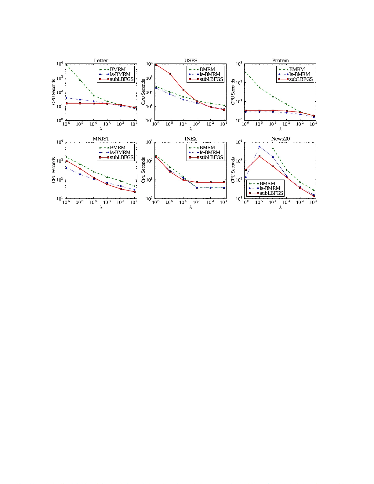
Journal of Mac hine Learning Researc h 11 (2010) 1–57 Submitted 11/08; Published -/10 A Quasi-Newton Approac h to Nonsmo oth Con v ex Optimization Problems in Mac hine Learning Jin Y u jin.yu@adelaide.edu.au Scho ol of Co mputer Scienc e The University o f A delaide A delaide SA 5005 , Austr alia S.V . N. Vish w anathan vishy@st a t.purdue.edu Dep artments of Statistics a nd Computer Scienc e Pur due University West L afayette, IN 4 7907-206 6 USA Simon G ¨ un ter guenter simon@hotmail.com DV Bern A G Nussb aum str asse 21, CH-3000 Bern 22, Switzerland Nicol N. Sc hraudolph jmlr@schraudolph.org adaptive to ols A G Canb err a ACT 2602, Austr alia Editor: Sathiya Keerthi Abstract W e extend the well-known BFGS quasi- Newton metho d and its memory-limited v ar ian t LBFGS to the optimization of nonsmooth conv ex o b jectives. This is done in a rigoro us fashion by generalizing three comp onents of B F GS to subdiﬀerentials: the lo cal quadratic mo del, the identiﬁcation o f a descent direction, and the W olfe line sear c h conditions. W e prov e that under s ome tec hnical conditions, the resulting s ubBF GS algorithm is globally conv er gen t in ob jectiv e function v alue. W e apply its memory-limited v ariant (subLBF GS) to L 2 -regular ized risk minim ization with the binar y hinge loss. T o extend our a lgorithm to the m ulticlass and multilabel settings, w e develop a ne w , eﬃcient, exact line sear c h algorithm. W e pr o ve its w orst-cas e time c o mplexit y bounds, and show that our line search can als o be used to extend a recently developed bundle method to the multiclass and m ultilab el settings. W e also apply the direction-ﬁnding component of our algor ithm to L 1 - regular iz ed r isk minimization with logistic loss. In all these contexts our metho ds perfor m comparable t o or better than sp ecialized state-of-the-a rt solvers on a num b er of publicly av ailable datasets. An op en source implementation o f our algorithms is freely a v ailable. Keyw ords: BFGS, V ariable Metric Metho ds, W o lfe Conditions, Subgradient, Risk Min- imization, Hinge Loss, Multicla ss, Multilab el, Bundle Methods, BMRM, OCAS, OWL-QN 1. In tro duction The BF GS quasi-Newton method ( No ce dal and W right , 19 99 ) and its memo ry-limited LBF GS v arian t are wid ely regarded a s the w orkhorses of smo oth n onlinear optimization d u e to their c  2010 Ji n Y u, S.V . N. Vishw anathan, Simon G ¨ un ter, and Nicol N. Schraud olph. Yu, Vishw ana than, G ¨ unter, and Schraudolph Figure 1: Geometric illustration of the W olfe conditions ( 4 ) and ( 5 ). com b in at ion of computational eﬃciency and go o d asymptotic co nv ergence. Given a smooth ob jectiv e function J : R d → R and a cur ren t iterate w t ∈ R d , BF GS forms a local quadratic mo del of J : Q t ( p ) := J ( w t ) + 1 2 p ⊤ B − 1 t p + ∇ J ( w t ) ⊤ p , (1) where B t ≻ 0 is a p ositiv e-deﬁn ite estimate of the inv erse Hessian of J , and ∇ J denotes the gradien t. Minimizing Q t ( p ) giv es the qu asi- Newton direction p t := − B t ∇ J ( w t ) , (2) whic h is used for the p aramet er up date: w t +1 = w t + η t p t . (3) The step size η t > 0 is normally d ete rmined by a lin e searc h ob eying the W olfe ( 1969 ) conditions: J ( w t +1 ) ≤ J ( w t ) + c 1 η t ∇ J ( w t ) ⊤ p t (suﬃcien t decrease) (4) and ∇ J ( w t +1 ) ⊤ p t ≥ c 2 ∇ J ( w t ) ⊤ p t (curv ature) (5) with 0 < c 1 < c 2 < 1. Figure 1 illus tr a tes these conditions geomet rically . Th e matrix B t is then mo diﬁed via the incrementa l rank-tw o up date B t +1 = ( I − ρ t s t y ⊤ t ) B t ( I − ρ t y t s ⊤ t ) + ρ t s t s ⊤ t , (6) where s t := w t +1 − w t and y t := ∇ J ( w t +1 ) − ∇ J ( w t ) denote the most r ec en t step along the optimization tra jectory i n parameter and gradient space, resp ectiv ely , and ρ t := ( y t ⊤ s t ) − 1 . The BF GS up date ( 6 ) enf orces the secan t equation B t +1 y t = s t . Given a d esce nt direction p t , the W olfe conditions ensure that ( ∀ t ) s ⊤ t y t > 0 and hence B 0 ≻ 0 = ⇒ ( ∀ t ) B t ≻ 0. 2 Quasi-Newton Appro ach to Nonsmooth Convex Optimiza tion Limited-memory BF GS (LBF GS, Liu and No cedal , 19 89 ) is a v arian t of BF GS designed for high-dimensional optimization problems where the O ( d 2 ) co st of sto ring and u pd ati ng B t w ould b e prohibitiv e. LBF GS appro ximates the quasi-Newton direction ( 2 ) directly from the last m p airs o f s t and y t via a matrix-free a pproac h, r educing the cost to O ( md ) space and time p er iteration, with m freely c hosen. There ha v e b een some attempts to app ly (L)BF GS directly to n onsmooth optimiza- tion problems, in the hop e that they would p erform w ell on nonsm o oth functions that are con v ex and diﬀerent iable almost ev eryw here. I ndeed, it h a s b een noted that in cases where BFGS ( r esp. LBF GS) does not encount er an y nonsmo oth p oin t, it often co nv erges to the optim um ( Lemarec hal , 1 982 ; Lewis and Overton , 2008a ). Ho we v er, Luk ˇ san and Vl ˇ cek ( 1999 ), Haarala ( 200 4 ), and Lewis and Overto n ( 200 8b ) also rep ort catastrophic failures of (L)BF GS on nonsmo oth f unctions. V arious ﬁ xes can b e used to av oid this problem, but only in an ad-ho c manner. Th erefore, subgradient-based approac hes suc h as su bgradien t d esce nt ( Nedi ´ c and Bertsek as , 2000 ) or bund le metho ds ( Joac him s , 2006 ; F ranc and Sonnenburg , 2008 ; T eo et al. , 200 9 ) ha v e gained considerable attent ion f or minimizing nonsmo oth ob jec- tiv es. Although a con v ex function might not b e diﬀeren tiable ev eryw here, a sub gradien t al- w a ys exists ( Hiriart-Urrut y and Lemar ´ ec hal , 1993 ). Let w b e a p oin t where a con vex function J is ﬁ nite. Then a subgradien t is the normal v ector of an y tangen tial supp ort- ing hyp erplane of J at w . F ormally , g is called a su bgradien t of J at w if and only if ( Hiriart-Urrut y and Lemar ´ ec hal , 1993 , Deﬁnition VI.1.2.1 ) ( ∀ w ′ ) J ( w ′ ) ≥ J ( w ) + ( w ′ − w ) ⊤ g . (7) The set of all subgradien ts at a point is c alled the sub diﬀeren tial, and is denoted ∂ J ( w ). If this set is not emp t y then J is said to b e sub diﬀer entiable at w . If it cont ains exactly one element, i.e. , ∂ J ( w ) = {∇ J ( w ) } , then J is d iﬀer entiable at w . Figure 2 p ro vides the geometric in terp reta tion of ( 7 ). The ai m of th is p ap er is to dev elop prin cipled and r obust quasi-Newton metho ds that are amenable to sub grad ients. This r esults in subBFGS and its m emory-limited v ariant subLBF GS, tw o new subgradient quasi-Newton m et ho ds th at are ap p lica ble to nonsmo oth con vex optimiza tion problems. In p articula r, we apply our algo rithms to a v arie t y of ma - c h ine lea rning p roblems, exploiting kno w ledge ab ou t the s ub diﬀeren tial of the binary hin ge loss and its generalizations to the multicla ss an d multi lab el settings. In the n ext secti on we motiv ate our work b y illustrating the diﬃculties of LBFGS on nonsmo oth functions, and th e adv ant age of incorp orating BF GS’ curv ature estimate in to the parameter up date. In S ection 3 w e dev elop our optimization algorithms generically , b efore discu s sing their applicati on to L 2 -regularized risk minimization with the hinge loss in S ect ion 4 . W e describ e a new eﬃcient algorithm to id en tify the nonsmo oth p oints of a one- dimensional p oin t wise maxim um of linear fu nctions in Section 5 , then use it to d ev elop an exact line searc h that extends our optimization algorithms to the m ulticlass and m ultilab el settings (Section 6 ). Section 7 compares and con trasts our work w it h other recen t eﬀorts in this area. W e report our exp erimen tal results on a n u m b er of public datasets in Section 8 , and conclude with a discu s sion and outlo ok in S ection 9 . 3 Yu, Vishw ana than, G ¨ unter, and Schraudolph Figure 2: Geometric in terp reta tion of subgradien ts. The dashed lines are tangen tial to the hinge function (solid b lue line); the slop es of these lines are sub gradien ts. 2. Motiv ation The application of s tand ard (L)BF GS to nonsmo oth optimization is p roblematic s in ce the quasi-Newton d irect ion generated at a nonsm o oth p oin t is not necessarily a descent direc- tion. Nev ertheless, BF GS’ inv erse Hessian estimate can pro vide an eﬀectiv e mo del of the o verall s h ape of a nonsmo oth ob jectiv e; incorp orat ing it in to the parameter up date can therefore b e b eneﬁcial. W e discuss these tw o asp ects of (L)BF GS to motiv ate our wo rk on dev eloping n ew quasi-Newton m etho ds that are amenable to su bgradien ts while pr eservin g the fast con ve rgence p rop ertie s of s tand ard (L)BF GS. 2.1 Problems of (L)BFGS on Nons mo oth Ob jectiv es Smo othness of the ob jectiv e fu nctio n is essential for classical (L)BF GS b ecause b oth the lo ca l quadratic model ( 1 ) a nd the W o lfe conditions ( 4 , 5 ) require the existence of the gra- dien t ∇ J at every p oin t. As p oin ted out b y Hiriart-Urrut y and Lemar ´ ec hal ( 1993 , Remark VI I I.2. 1.3), ev en though nonsmo ot h con v ex functions are d iﬀeren tiable ev erywhere except on a set of Leb esgue measure zero, it is u n wise to just use a smooth optimizer on a nons- mo oth conv ex p roblem und er the assumption that “ it should w ork almost surely .” Belo w w e illustrate this on b oth a to y e xample and real-w orld mac h ine learnin g pr oblems. 2.1.1 A Toy Example The follo wing simple example demonstrates th e pr o blems f ac ed b y BF GS wh en w ork in g with a nonsmo oth ob jectiv e function, and ho w o ur sub grad ient BF GS (su bBF GS) metho d (to b e introd uced in Section 3 ) with exact line searc h o v ercomes th ese pr oblems. Consid er the task of m inimizing f ( x, y ) = 10 | x | + | y | (8) 4 Quasi-Newton Appro ach to Nonsmooth Convex Optimiza tion Figure 3: Left: th e nonsmo oth con v ex function ( 8 ); optimization tra jectory of BF GS with inexact line searc h (cent er) a nd subBF GS (righ t) on this function. with resp ect to x and y . Clearly , f ( x, y ) is conv ex but n on s mooth, with th e m inim um lo ca ted at (0 , 0) ( Figure 3 , left). It is sub diﬀeren tiable wh enev er x or y is z ero: ∂ x f (0 , · ) = [ − 10 , 10] a nd ∂ y f ( · , 0) = [ − 1 , 1] . (9) W e call suc h lines of sub diﬀeren tiabilit y in parameter space hinges . W e can minimize ( 8 ) with the stand ard BF GS algorithm, employi ng a bac ktr acking line searc h ( No ce dal and W righ t , 199 9 , Pro cedure 3.1) that starts with a step size that ob eys the curv ature condition ( 5 ), then exp on entially deca ys it until b oth W olfe conditions ( 4 , 5 ) are satisﬁed. 1 The curv ature condition forces BF GS to jump across at least one hinge, th us ensuring that the gradien t displacemen t v ector y t in ( 6 ) is non-zero; this preven ts BF GS from div erging. Moreo ver, w ith such an inexact line searc h BF GS will generally not step on an y hinges directly , th us a voiding (in an ad-ho c manner) the p r oblem of n on-diﬀeren tia- bilit y . Although this algorithm quic kly decreases the ob jectiv e fr om the starting p oin t (1 , 1), it is then slo wed do w n b y heavy oscil lations arou n d the optimum (Figure 3 , cen ter), caused b y the utter mismatc h b et w een BF GS’ quadratic m odel and the actual function. A generally sensible strategy is to use an exact line searc h that ﬁnds the optim um along a given descen t direction ( cf. Section 4.2.1 ). Ho wev er, t his line optim um will often lie on a hinge (as it do es in our to y example), where the function is n ot diﬀerent iable. If an arb itrary subgradient is su pplied ins te ad, the BF GS up date ( 6 ) can pro duce a search direction whic h is not a descen t direction, causing the next line searc h to fail. In our to y example, standard BF GS with exact line searc h consisten tly fails after the ﬁrst step, whic h ta k es it to the h inge at x = 0. Unlik e standard BF GS, our subBFGS metho d can h andle hinges and thus reap the b eneﬁts of an exact line search. As Figure 3 (right) shows, once the ﬁrst iteration of subBF GS lands it on the hinge a t x = 0, its direction-ﬁnding routine (Algorithm 2 ) ﬁnds a descen t d ir ec tion for the n ext step. In fact, o n t his simple example Algo rithm 2 yields a v ector w ith zero x component, w h ic h ta k es subBF GS straig ht to the optim u m at the second step. 2 1. W e set c 1 = 10 − 3 in ( 4 ) an d c 2 = 0 . 8 in ( 5 ), and used a deca y factor of 0.9. 2. This is ac hieved for any choice of initial subgradien t g (1) (Line 3 of A lg orithm 2 ). 5 Yu, Vishw ana than, G ¨ unter, and Schraudolph Figure 4: P er f ormance of subLBFGS (solid) and standard LBFGS with exact (dashed) and inexact (dotted) line s earch metho ds on samp le L 2 -regularized r isk minimization problems w ith the binary (left and cen ter) and m ulticlass hinge losses (right). LBF GS with exact line searc h (dashed) fails after 3 iterations (marked as × ) on the Leuk emia dataset (left). 2.1.2 Typical Nons mooth Optimiza tion Problems i n Machine Le arning The prob lems faced b y smo oth qu a si-Newton metho ds on nonsmo oth ob jectiv es are not only encoun tered in clev erly constru cted to y examp les, but also in r eal-wo rld applicatio ns. T o sho w this, w e apply LBF GS to L 2 -regularized r isk minimizatio n problems ( 35 ) with binary hinge loss ( 36 ), a typical nonsm ooth optimization problem encounte red in machine learning. F or this particular ob jectiv e function, an exact line search is c heap and easy to compu te (see Section 4.2.1 for details). Figure 4 ( left & cente r) sho ws the b ehavior of LBF GS with this exact line searc h (LBF GS-LS ) on tw o datasets, n amel y Leuk emia and Real-sim. 3 It can b e seen that LBF GS-LS conv erges o n Re al-sim but d iv erges o n the Leuk emia dataset. This is b ecause using an exact line searc h on a nonsmo oth ob jectiv e fun cti on increases the c h ance of landing on nonsm o oth p oin ts, a situation that standard BF GS ( r esp. LBFGS) is not designed to deal with. T o p rev ent (L)BF GS ’ sudden breakdo wn , a sc heme that ac tiv ely a voids nonsmo oth p oin ts must b e used. One suc h p ossibilit y is to use an inexact line searc h that obeys the W olfe co nditions. Here w e used an eﬃcien t inexact line searc h that uses a cac hing sc heme sp eciﬁcally designed for L 2 -regularized hinge loss ( cf. end o f Section 4.2 ). This implemen tation of LBF GS (LBF GS-ILS) conv erges on b oth datasets sho wn here but ma y fail on others. It is also slo wer, due to the inexactness of its line search. F or the m ulticlass hinge loss ( 49 ) w e encoun ter another problem: if w e follo w the usual practice of initializing w = 0 , whic h happ ens to b e a non-diﬀerentiable p oin t, th en LBF GS stalls. One wa y to get aroun d this is to force LBFG S to tak e a unit step along its searc h direction to escap e this nonsm ooth p oin t. Ho w ev er, as can b e seen on the Letter dataset 3 in Figure 4 (righ t), suc h an ad-ho c ﬁx increases the v al ue of the ob jectiv e ab o v e J ( 0 ) (solid horizon tal line), and it tak es several CPU seconds for the optimizers to reco ver from this. In all cases sho wn in Figure 4 , our sub gradien t LBF GS (sub LBF GS) metho d (as will b e in tro duced later) p erforms comparable to or b etter than the b est implemen tation of LBF GS. 3. Descriptions of these datasets can be found in Section 8 . 6 Quasi-Newton Appro ach to Nons mooth Convex Optimiza tion Figure 5: P er f ormance of subLBFG S, GD, and subGD on sample L 2 -regularized risk min- imization problems with binary (left), multiclass (cen ter), and multilabel (righ t) hinge losses. 2.2 Adv an tage of I nco rp orating BFGS’ C urv ature Estimate In machine learnin g one often encounters L 2 -regularized risk m inimiza tion problems ( 35 ) with v arious hinge losses ( 36 , 49 , 64 ). S ince the Hessian of those ob jectiv e fun ctio ns at dif- feren tiable p oin ts equals λ I (wh ere λ is the regularization constan t), one migh t b e te mpted to argue that for suc h p roblems, BF GS’ approximati on B t to the in v erse Hessian should b e simply set to λ − 1 I . This would redu ce th e quasi-Newton direction p t = − B t g t , g t ∈ ∂ J ( w t ) to simply a scale d su b gradien t direction. T o c hec k if d oing so is b eneﬁcial, w e compared the p erformance of our subLBFG S metho d with t wo implementat ions of subgradient descent : a v anilla gradient d esce nt metho d (denoted GD) that u ses a random su bgradien t for its parameter up date, and an impr ov ed subgradient descen t metho d (denoted subGD) whose parameter is u p d ate d in the direction pro duced by ou r direction-ﬁnding routine (Algorithm 2 ) with B t = I . All algorithms used exact line searc h, except that GD to ok a unit step for the ﬁrs t up date in order to av oid the nonsmo oth p oin t w 0 = 0 ( cf. the discussion in Section 2.1 ). As can b e seen in Figure 5 , on all sample L 2 -regularized hinge loss m inimizat ion pr oblems, sub LBF GS (solid) con verges signiﬁcan tly faster than GD (dotted) and su bGD (d ashed). T his indicates that BFG S’ B t matrix is able to mo del the ob jectiv e function, includ ing its hinges, b etter than simp ly setting B t to a scaled id en tit y matrix. W e b el iev e that BF GS’ curv ature up date ( 6 ) plays an imp ortan t role in the p erform ance of s ubLBF GS seen in Figure 5 . Recall that ( 6 ) satisﬁes the secan t condition B t +1 y t = s t , where s t and y t are d isp lac emen t vecto rs in parameter and gradien t space, resp ectiv ely . The secan t condition in fact implemen ts a ﬁnite diﬀe r enc i ng sc heme: f or a one-dimensional ob jectiv e fun ct ion J : R → R , we hav e B t +1 = ( w + p ) − w ∇ J ( w + p ) − ∇ J ( w ) . (10) Although the original motiv ation b ehind the secan t condition was to approxima te the inv erse Hessian, the ﬁ nite d iﬀerencing sc heme ( 10 ) allo w s BFGS to mo del th e global curv ature ( i.e. , o verall shap e) of the ob j ectiv e function from ﬁrst-order information. F or instance, Figure 6 7 Yu, Vishw ana than, G ¨ unter, and Schraudolph Figure 6: BF GS’ quadratic appr o ximation to a piecewise linear fun ct ion (left), and its es- timate of the gradien t of this function (righ t). (left) s h o ws that the BF GS quadr at ic mo del 4 ( 1 ) ﬁ ts a piecewise linear fu nctio n quite w ell despite the fact that the actual Hessian in this case is zero almost ev erywhere, and inﬁnite (in the limit) at nonsmo oth p oint s. Figure 6 (righ t) rev eals that BF GS captures the global trend of the gradien t rather than its in ﬁnitesimal v ariation, i.e. , the Hessian. This is b eneﬁcial for n onsmooth problems, wh ere Hessian do es not fu lly represent th e o verall curv ature of the ob jectiv e fu n cti on. 3. Subgradien t BF GS Metho d W e mo dify the stand ard BF GS algorithm to deriv e our new algorithm (su bBF GS, Algo- rithm 1 ) for nonsmo oth c on v ex optimization, and its memory-limited v arian t (subLBF GS). Our mo diﬁcations can b e group ed into three areas, wh ich w e elab orate on in turn: gener- alizing the lo cal quad r ati c mo del, ﬁnding a descent dir ec tion, and ﬁ nding a step size that ob eys a subgradient r eform ulation of the W olfe conditions. W e then sho w that our algo- rithm’s estimate of the inv erse Hessian has a b ounded sp ectrum, wh ic h allo ws us to pr o v e its con vergence. 3.1 Generalizing the Lo cal Q uadratic Mo del Recall that BF GS assumes that the ob jectiv e function J is diﬀerent iable eve rywhere so that at the current iterate w t it can construct a lo cal quadratic mo del ( 1 ) of J ( w t ). F or a nonsmo oth ob jectiv e function, such a mo del b ecomes am biguous at non-diﬀerent iable p oin ts (Figure 7 , left). T o resolv e the ambiguit y , we could simply replace the gradien t ∇ J ( w t ) in ( 1 ) with an arbitrary sub gradien t g t ∈ ∂ J ( w t ). Ho wev er, as will b e discussed later, the resulting quasi-Newton direction p t := − B t g t is n ot n ec essarily a descent direction. T o address this fu ndamen tal m o deling p roblem, we ﬁ rst generalize the lo cal qu adratic mo del 4. F or ease of exp osition, the model was constructed at a diﬀeren tiable point. 8 Quasi-Newton Appro ach to Nons mooth Convex Optimiza tion Algorithm 1 S ubgradien t BF GS (subBF GS) 1: Initialize: t := 0 , w 0 = 0 , B 0 = I 2: Set: direction-ﬁnding tolerance ǫ ≥ 0, iteration limit k max > 0, lo wer b ound h > 0 on s ⊤ t y t y ⊤ t y t ( cf. discussion in Section 3.4 ) 3: Compu te subgradient g 0 ∈ ∂ J ( w 0 ) 4: while not con verge d do 5: p t = de scentDirection ( g t , ǫ, k max ) (Algorithm 2 ) 6: if p t = failure t hen 7: Return w t 8: end if 9: Find η t that ob eys ( 25 ) and ( 26 ) ( e.g. , Algorithm 3 or 5 ) 10: s t = η t p t 11: w t +1 = w t + s t 12: Cho ose s ubgradien t g t +1 ∈ ∂ J ( w t +1 ) : s ⊤ t ( g t +1 − g t ) > 0 13: y t := g t +1 − g t 14: s t := s t + max  0 , h − s ⊤ t y t y ⊤ t y t  y t (ensure s ⊤ t y t y ⊤ t y t ≥ h ) 15: Up date B t +1 via ( 6 ) 16: t := t + 1 17: end while ( 1 ) as follo ws: Q t ( p ) := J ( w t ) + M t ( p ) , w h ere M t ( p ) := 1 2 p ⊤ B − 1 t p + sup g ∈ ∂ J ( w t ) g ⊤ p . (11) Note that where J is diﬀeren tiable, ( 11 ) reduces to the familiar BF GS quadratic m odel ( 1 ). A t n o n-diﬀerentia ble p oin ts, ho w ev er, th e mo del is no longer quadr at ic, as the supr em um ma y b e attained at diﬀeren t elemen ts of ∂ J ( w t ) for diﬀeren t directions p . I nstead it can b e view ed as the tighte st pseudo-quadr ati c ﬁt to J at w t (Figure 7 , right ). Although the lo ca l mo del ( 11 ) of s ubBF GS is n on s mooth, it only incorp orates non -d iﬀe renti al points pr ese nt at the curr en t lo cation; all others are smo othly approximat ed by the quasi-Newton mechanism. Ha ving constructed the mo del ( 11 ), we can minimize Q t ( p ), or equiv alen tly M t ( p ): min p ∈ R d 1 2 p ⊤ B − 1 t p + sup g ∈ ∂ J ( w t ) g ⊤ p ! (12) to obtain a searc h dir ec tion. W e no w show that solving ( 12 ) is closely related to the prob lem of ﬁnding a normalize d ste ep est desc ent direction. A n ormaliz ed steep est descen t dir ection is deﬁned as the solution to the f ol lo w ing p r oblem ( Hiriart-Urrut y and Lemar ´ ec h al , 1993 , Chapter VI I I): min p ∈ R d J ′ ( w t , p ) s.t. | | | p | | | ≤ 1 , (13) 9 Yu, Vishw ana than, G ¨ unter, and Schraudolph Figure 7: Left: selecting arbitrary sub gradien ts yields m a ny p ossible quadr atic mo dels (dot- ted lines) f or the ob jectiv e (solid blue line) at a sub diﬀerenti able p oin t. Th e mo d- els were built by k eeping B t ﬁxed, but selecting random s ubgradien ts. Righ t: the tigh test pseudo-quadr atic ﬁt ( 11 ) (b old red d ashes); note that it is not a qu adratic . where J ′ ( w t , p ) := lim η ↓ 0 J ( w t + η p ) − J ( w t ) η is the d irect ional deriv ativ e of J at w t in direction p , and | | | · | | | is a norm deﬁned on R d . In other w ords, the normalized steepest descent direction is the d ir ec tion of b ound ed n orm along whic h the maxim um rate of d ec rease in the ob jectiv e f unction v alue is ac h ie v ed. Using the prop erty: J ′ ( w t , p ) = su p g ∈ ∂ J ( w t ) g ⊤ p ( Bertsek as , 1999 , Prop osition B.24.b), we can rewrite ( 13 ) as: min p ∈ R d sup g ∈ ∂ J ( w t ) g ⊤ p s.t. | | | p | | | ≤ 1 . (14) If the m a trix B t ≻ 0 as in ( 12 ) is used to d eﬁne the norm | | | · | | | as | | | p | | | 2 := p ⊤ B − 1 t p , (15) then the solution to ( 14 ) p oints to the same direction as that obtained b y minimizing our pseudo-quadratic mo del ( 12 ). T o see this, w e write the L a grangian of the constrained minimization problem ( 14 ): L ( p , α ) := α p ⊤ B − 1 t p − α + sup g ∈ ∂ J ( w t ) g ⊤ p = 1 2 p ⊤ (2 α B − 1 t ) p − α + sup g ∈ ∂ J ( w t ) g ⊤ p , (16) where α > 0 is a Lagrangian multiplier. It is easy to see from ( 16 ) th at minimizing the Lagrangian function L with resp ect to p is equiv alen t to solving ( 12 ) with B − 1 t scaled by a scalar 2 α , imp lying that the steep est descent d ir ec tion obtained b y solving ( 14 ) with the 10 Quasi-Newton Appro ach to Nons mooth Convex Optimiza tion w eigh ted norm ( 15 ) only diﬀers in length from the search direction obtained by s o lving ( 12 ). Therefore, our search direction is e ssenti ally an unn omalized steep est descen t directio n with resp ect to the we igh ted norm ( 15 ). Ideally , w e w ould lik e to solv e ( 12 ) to obtain the b est searc h direction. This is generally in tractable due to the presence a s uprem u m o v er the en tire su b d iﬀe renti al set ∂ J ( w t ). In man y m a c hine learning pr oblems, how ev er, ∂ J ( w t ) has some sp ecial structure that simp liﬁes the calculation of that supremum. In p articula r, th e sub diﬀerential of all th e problems considered in this pap er is a con v ex and compact p olyhedron c h arac terised as the con vex h ull of its extreme p oin ts. This dramatically reduces the cost of calculating sup g ∈ ∂ J ( w t ) g ⊤ p since the su prem um can only b e at tained at an extreme p oint of the p olyhedral set ∂ J ( w t ) ( Bertsek as , 1999 , Prop osition B.21c). In what f ol lo w s, w e dev elop an iterativ e p rocedur e that is guarantee d to ﬁnd a qu a si-Newton descen t direction, assuming an oracle that supp lies arg sup g ∈ ∂ J ( w t ) g ⊤ p for a giv en direction p ∈ R d . Eﬃcient oracles f or this p urp ose can b e deriv ed for man y mac hine learning settings; we pro vides suc h oracle s for L 2 -regularized risk minimization with the binary h inge loss (Sect ion 4.1 ), multicla ss and multila b el hinge lo sses (Section 6 ), and L 1 -regularized logistic loss (Section 8.4 ). 3.2 Finding a Descen t Direction A direction p t is a d esce nt d irect ion if and on ly if g ⊤ p t < 0 ∀ g ∈ ∂ J ( w t ) ( Hiriart-Urrut y and Lemar ´ ec hal , 1993 , Theorem VI I I.1.1.2), or equiv alen tly sup g ∈ ∂ J ( w t ) g ⊤ p t < 0 . (17) F or a smo oth con vex function, the quasi-Newto n direction ( 2 ) is alwa ys a d esce n t d irect ion b ecause ∇ J ( w t ) ⊤ p t = −∇ J ( w t ) ⊤ B t ∇ J ( w t ) < 0 holds due to the p ositivit y of B t . F or nonsmo oth fun ct ions, h o w ev er, the quasi-Newton direction p t := − B t g t for a giv en g t ∈ ∂ J ( w t ) ma y not f ulﬁll the descen t condition ( 17 ) , m aking it imp ossible to ﬁ n d a step size η > 0 that ob eys the W o lfe conditions ( 4 , 5 ), thus causing a failure of the line searc h. W e now pr ese nt an iterativ e approac h to ﬁnding a quasi-Newton desc ent direction. Our goal is to minimize the pseudo-quadratic mo del ( 11 ), or equiv alen tly minimize M t ( p ). Inspired by bu ndle metho ds ( T eo et al. , 2009 ), w e ac hiev e this b y minimizing conv ex lo wer b ounds of M t ( p ) th at are d esigned to pr og ressiv ely approac h M t ( p ) o v er iterations. A t iteration i we build the follo wing con v ex lo w er b ound on M t ( p ): M ( i ) t ( p ) := 1 2 p ⊤ B − 1 t p + sup j ≤ i g ( j ) ⊤ p , (18) where i, j ∈ N and g ( j ) ∈ ∂ J ( w t ) ∀ j ≤ i . Give n a p ( i ) ∈ R d the lo we r b ound ( 18 ) is successiv ely tigh tened b y computing g ( i +1) := arg sup g ∈ ∂ J ( w t ) g ⊤ p ( i ) , (19) 11 Yu, Vishw ana than, G ¨ unter, and Schraudolph Algorithm 2 p t = de scentDirection ( g (1) , ǫ, k max ) 1: input (sub)gradient g (1) ∈ ∂ J ( w t ), tolerance ǫ ≥ 0, iteration limit k max > 0, and an oracle to calculat e arg sup g ∈ ∂ J ( w ) g ⊤ p for an y give n w and p 2: output descen t direction p t 3: Initialize: i = 1 , ¯ g (1) = g (1) , p (1) = − B t g (1) 4: g (2) = arg sup g ∈ ∂ J ( w t ) g ⊤ p (1) 5: ǫ (1) := p (1) ⊤ g (2) − p (1) ⊤ ¯ g (1) 6: while ( g ( i +1) ⊤ p ( i ) > 0 or ǫ ( i ) > ǫ ) and ǫ ( i ) > 0 and i < k max do 7: µ ∗ := min h 1 , ( ¯ g ( i ) − g ( i +1) ) ⊤ B t ¯ g ( i ) ( ¯ g ( i ) − g ( i +1) ) ⊤ B t ( ¯ g ( i ) − g ( i +1) ) i ; cf. ( 111 ) 8: ¯ g ( i +1) = (1 − µ ∗ ) ¯ g ( i ) + µ ∗ g ( i +1) 9: p ( i +1) = (1 − µ ∗ ) p ( i ) − µ ∗ B t g ( i +1) ; cf. ( 86 ) 10: g ( i +2) = arg sup g ∈ ∂ J ( w t ) g ⊤ p ( i +1) 11: ǫ ( i +1) := min j ≤ ( i +1)  p ( j ) ⊤ g ( j +1) − 1 2 ( p ( j ) ⊤ ¯ g ( j ) + p ( i +1) ⊤ ¯ g ( i +1) )  12: i := i + 1 13: end while 14: p t = argmin j ≤ i M t ( p ( j ) ) 15: if sup g ∈ ∂ J ( w t ) g ⊤ p t ≥ 0 then 16: return failure; 17: else 18: return p t . 19: end if suc h that M ( i ) t ( p ) ≤ M ( i +1) t ( p ) ≤ M t ( p ) ∀ p ∈ R d . Here we set g (1) ∈ ∂ J ( w t ) arb itrarily , and assume that ( 19 ) is pr ovided b y an oracle ( e.g. , as describ ed in Section 4.1 ). T o solv e min p ∈ R d M ( i ) t ( p ), w e rewrite it as a constrained optimization problem: min p ,ξ  1 2 p ⊤ B − 1 t p + ξ  s.t. g ( j ) ⊤ p ≤ ξ ∀ j ≤ i. (20) This problem can b e solv ed exactly via q u adratic programming, but doing so ma y incur substanti al computational exp ense. In stea d we adopt an alternativ e approac h (Algorithm 2 ) whic h d oes not sol v e ( 20 ) to optimali t y . The k ey idea is to write the p rop osed descen t direc- tion at iteration i + 1 as a con vex combination of p ( i ) and − B t g ( i +1) (Line 9 o f Algorithm 2 ); and as w ill b e sho wn in App endix B , the returned searc h d irect ion tak es the form p t = − B t ¯ g t , (21) where ¯ g t is a sub gradien t in ∂ J ( w t ) that allo ws p t to satisfy the descent condition ( 17 ). The optimal co nv ex com b inatio n co eﬃcie nt µ ∗ can b e computed exa ctly (Line 7 of Alg orithm 2 ) using an argument based on maximizing the dual ob jectiv e of M t ( p ); see App endix A f or details. The w eak dualit y theorem ( Hiriart-Urrut y and Lemar ´ ec hal , 1993 , Theorem XI I .2 .1.5) states that the optimal p rimal v alue is no less than an y du al v alue, i.e. , if D t ( α ) is the dual of M t ( p ), th en min p ∈ R d M t ( p ) ≥ D t ( α ) holds for all feasible dual solutions α . Therefore, 12 Quasi-Newton Appro ach to Nons mooth Convex Optimiza tion b y iterativ ely increasing the v alue of th e dual ob j ective we close the gap to optimalit y in the primal. Based on this argum en t, we u se the follo w in g upp er b ound on the d ualit y gap as our m easur e of progress: ǫ ( i ) := min j ≤ i h p ( j ) ⊤ g ( j +1) − 1 2 ( p ( j ) ⊤ ¯ g ( j ) + p ( i ) ⊤ ¯ g ( i ) ) i ≥ min p ∈ R d M t ( p ) − D t ( α ∗ ) , (22) where ¯ g ( i ) is an aggregated subgradien t (Lin e 8 of Algorithm 2 ) whic h lie s in the conv ex h u ll of g ( j ) ∈ ∂ J ( w t ) ∀ j ≤ i , and α ∗ is the optimal du al solution; equations 87 – 89 in App endix A pro vide in termed iate steps that lead to the in equalit y in ( 22 ). Theorem 7 (App end ix B ) sho ws th at ǫ ( i ) is monotonically decreasing, lea ding us to a practical stopping criterion (Line 6 of Algorithm 2 ) f or our direction-ﬁnding pro cedure. A detailed deriv ation of Algorithm 2 is giv en in App endix A , where we also pr o v e that at a non-optimal iterate a direction-ﬁndin g tolerance ǫ ≥ 0 exists such that the searc h direction p rodu ce d by Algorithm 2 is a d esc en t direction; in App endix B we prov e that Algorithm 2 conv erges to a solution with precision ǫ in O (1 /ǫ ) iterations. Our pro ofs are based on the assumption that the sp ectrum (eigen v alues) of BF GS’ appro xim ation B t to the inv erse Hessian is b ounded from ab o ve and b elo w. This is a reasonable assumption if simple safeguards suc h as th ose d escribed in Section 3.4 are emplo yed in th e practical implemen tation. 3.3 Subgradien t Line Search Giv en the current iterate w t and a searc h d irecti on p t , the task of a line searc h is to ﬁ nd a step size η > 0 wh ic h reduces the ob jectiv e function v alue along the line w t + η p t : minimize Φ( η ) := J ( w t + η p t ) . (23) Using the c hain ru le, w e can write ∂ Φ( η ) := { g ⊤ p t : g ∈ ∂ J ( w t + η p t ) } . (24) Exact line searc h ﬁnd s the optimal step size η ∗ b y minimizing Φ( η ), suc h that 0 ∈ ∂ Φ( η ∗ ); inexact line searc h es solve ( 23 ) ap p ro ximately while enforcing conditions designed to ensure con vergence. The W o lfe conditions ( 4 ) and ( 5 ), for instance, ac hiev e this by guarante eing a suﬃcient d ecrea se in the v alue of th e ob jectiv e and excluding pathologica lly small step sizes, resp ectiv ely ( W olfe , 1969 ; No cedal and W righ t , 1999 ). The original W o lfe conditions, ho w ev er, require the ob jectiv e function to b e smo ot h; to extend them to n on s mooth con vex problems, w e prop ose the follo wing sub gradien t reform ulation: J ( w t +1 ) ≤ J ( w t ) + c 1 η t sup g ∈ ∂ J ( w t ) g ⊤ p t (suﬃcien t decrease) (25) and sup g ′ ∈ ∂ J ( w t +1 ) g ′⊤ p t ≥ c 2 sup g ∈ ∂ J ( w t ) g ⊤ p t , (curv ature) (26) where 0 < c 1 < c 2 < 1. Figure 8 illustrates ho w these conditions enforce ac ceptance of non- trivial step sizes that decrease th e ob jectiv e function v alue. In Ap p end ix C we formally sh o w that for an y given descen t direction we can a lw a ys ﬁnd a positive step size that s at isﬁes ( 25 ) 13 Yu, Vishw ana than, G ¨ unter, and Schraudolph Figure 8: Geometric illustration of the subgradient W olfe conditions ( 25 ) an d ( 26 ) . Solid disks are sub diﬀeren tiable p oin ts; the slop es of dashed lines are indicated. and ( 26 ). Moreo ve r, App endix D shows that the su ﬃcie nt decrease condition ( 25 ) pro vides a necessary condition for the global conv ergence of subBFGS. Emplo ying an exact line searc h is a common strategy to sp eed up con vergence, b ut it drastically increases the probabilit y of landing on a non-diﬀeren tiable p oin t (as in Figure 4 , left). I n order to leve rage the fast con v ergence pro vided by an exact lin e searc h, one m ust therefore use an op timizer that can hand le subgradients, lik e our sub BFGS. A natural q u estio n to ask is whether the optimal step size η ∗ obtained by an exact line searc h satisﬁes the r eform ulated W olfe conditions ( r esp. the standard W olfe conditions when J is sm ooth). T h e answer is no: dep ending on the c h oi ce of c 1 , η ∗ ma y v iolate the suﬃcien t decrease condition ( 25 ). F or the function sho wn in Figure 8 , for ins ta nce, w e can increase the v alue of c 1 suc h that the acceptable int erv al for the step size exclud es η ∗ . In practice one can set c 1 to a small v alue, e . g. , 10 − 4 , to prev en t this from happ ening. The curv ature cond iti on ( 26 ), on the other hand, is alw a ys satisﬁed by η ∗ , as long as p t is a descen t direction ( 17 ): sup g ′ ∈ J ( w t + η ∗ p t ) g ′⊤ p t = sup g ∈ ∂ Φ( η ∗ ) g ≥ 0 > sup g ∈ ∂ J ( w t ) g ⊤ p t (27) b ecause 0 ∈ ∂ Φ( η ∗ ). 3.4 Bounded Sp ectrum of SubBF GS’ Inv erse Hessian Estimate Recall fr om S ect ion 1 that to ensur e p ositivit y of BF GS ’ estimate B t of th e in v erse Hessia n, w e m ust ha ve ( ∀ t ) s ⊤ t y t > 0. Extend in g this condition to nonsmo oth fu n ctio ns, w e require ( w t +1 − w t ) ⊤ ( g t +1 − g t ) > 0 , wher e g t +1 ∈ ∂ J ( w t +1 ) and g t ∈ ∂ J ( w t ) . (28) 14 Quasi-Newton Appro ach to Nons mooth Convex Optimiza tion If J is strongly con v ex, 5 and w t +1 6 = w t , then ( 28 ) holds for an y c hoice of g t +1 and g t . 6 F or general conv ex functions, g t +1 need to b e chosen (Line 12 of Algorithm 1 ) to satisfy ( 28 ). The existence of suc h a subgradient is guarant eed by the con v exit y of th e ob j ec tiv e function. T o see th is, w e ﬁrst use th e fact that η t p t = w t +1 − w t and η t > 0 to rewrite ( 28 ) as p ⊤ t g t +1 > p ⊤ t g t , w here g t +1 ∈ ∂ J ( w t +1 ) and g t ∈ ∂ J ( w t ) . (29) It follo w s from ( 24 ) that b oth sides of inequalit y ( 29 ) are s u bgradien ts of Φ( η ) at η t and 0, r espectiv ely . The monotonic prop ert y of ∂ Φ( η ) giv en in Th eo rem 1 (b elo w) ensur es that p ⊤ t g t +1 is no less than p ⊤ t g t for an y choice of g t +1 and g t , i.e. , inf g ∈ ∂ J ( w t +1 ) p ⊤ t g ≥ sup g ∈ ∂ J ( w t ) p ⊤ t g . (30) This means that the only case where inequalit y ( 29 ) is violated is wh en b oth terms of ( 30 ) are equal, and g t +1 = arg inf g ∈ ∂ J ( w t +1 ) g ⊤ p t and g t = arg sup g ∈ ∂ J ( w t ) g ⊤ p t , (31) i.e. , in this case p ⊤ t g t +1 = p ⊤ t g t . T o a v oid this, w e simply need to set g t +1 to a d iﬀeren t subgradient in ∂ J ( w t +1 ). Theorem 1 ( Hiriart-Urrut y and Lemar ´ ec hal , 1993 , T heorem I.4.2.1) L et Φ b e a one-dimensional c onvex fu nction on its domain, then ∂ Φ( η ) is incr e asing in the sense that g 1 ≤ g 2 whenever g 1 ∈ ∂ Φ( η 1 ) , g 2 ∈ ∂ Φ( η 2 ) , and η 1 < η 2 . Our conv ergence analysis f or the direction-ﬁnding pro cedure (Algorithm 2 ) as well as the global conv ergence pr oof of su b BF GS in App end ix D r equire the sp ectrum of B t to b e b ounded fr om ab o ve and b elo w by a p ositiv e scalar: ∃ ( h , H : 0 < h ≤ H < ∞ ) : ( ∀ t ) h  B t  H . (32) F rom a theoretica l p oint of view it is diﬃcult to guaran tee ( 32 ) ( Nocedal and W r igh t , 1999 , page 212) , but based on the fact th at B t is an appro ximation to the in verse Hessian H − 1 t , it is reasonable to exp ec t ( 32 ) to b e true if ( ∀ t ) 1 /H  H t  1 /h. (33) Since BF GS “senses” the Hessian via ( 6 ) only through the p aramete r and gradient displace- men ts s t and y t , we can tr an s la te the b ounds on the sp ectrum of H t in to conditions that only in volv e s t and y t : ( ∀ t ) s ⊤ t y t s ⊤ t s t ≥ 1 H and y ⊤ t y t s ⊤ t y t ≤ 1 h , w ith 0 < h ≤ H < ∞ . (34) 5. If J is strongl y con vex, then ( g 2 − g 1 ) ⊤ ( w 2 − w 1 ) ≥ c k w 2 − w 1 k 2 , with c > 0 , g i ∈ ∂ J ( w i ) , i = 1 , 2. 6. W e found empirica lly that n o qu ali tative d iﬀerence b etw een using random subgradients versus c ho osing a p artic ular subgradien t w hen updating the B t matrix. 15 Yu, Vishw ana than, G ¨ unter, and Schraudolph Figure 9: Con v ergence of s ubLBF GS in ob jectiv e function v alue on s amp le L 2 -regularized risk minimization problems with b inary (left) and multicla ss (righ t) h inge losses. This tec hn ique is used in ( No ce dal and W right , 1999 , Theorem 8.5). If J is strongly con v ex 5 and s t 6 = 0 , then th ere exists an H suc h that the left inequalit y in ( 34 ) holds. On general con vex functions, one can skip BF GS’ curv ature up date if ( s ⊤ t y t / s ⊤ t s t ) falls b elo w a thresh- old. T o establish the second inequalit y , we add a fraction of y t to s t at L in e 14 of Algorithm 1 (though this mo diﬁcation is n ev er actually in v ok ed in our exp eriments of Section 8 , wh ere w e set h = 10 − 8 ). 3.5 Limited-Memory Subgradient BF GS It is straight forwa rd to implement an LBFG S v arian t of ou r subBF GS algo rithm: we simp ly mo dify Algorithms 1 and 2 to compu te all pro ducts b et wee n B t and a vec tor by means of the standard LBF GS matrix-free sc heme ( No ce dal and W right , 1999 , Algorithm 9.1). W e call the resulting algorithm subLBF GS . 3.6 Conv ergence of Subgradien t (L)BFGS In S ec tion 3.4 we ha v e sh o wn that the sp ectrum of subBFGS’ inv erse Hessian estimate is b ounded. F rom this and other tec hnical assu mptions, w e prov e in App end ix D that sub - BF GS is globally conv ergen t in ob jectiv e function v alue, i.e. , J ( w ) → inf w J ( w ). Moreo v er, in App end ix E w e s ho w that su bBF GS con v erges f or all counte rexamples we could ﬁnd in the literature used to illustrate the non-con v ergence of existing optimization metho ds on nonsmo oth p roblems. W e h a v e also examined th e con v ergence of su b LBF GS empirically . In most of our exp erimen ts of Section 8 , w e observ e that after an in iti al transient, sub LBF GS observes a p erio d of linear con vergence, until close to the optimum it exhibits sup erlinear con v ergence b eha vior. This is illustrated in Figure 9 , where we plot (on a log scale) the excess ob jectiv e 16 Quasi-Newton Appro ach to Nons mooth Convex Optimiza tion function v alue J ( w t ) ov er its “optim um” J ∗ 7 against the iteration num b er in t wo t ypical runs. T h e same kind of con v ergence b eha vior w as observ ed by Lewis and Ov erton ( 2008a , Figure 5.7), who applied the classical BF GS algorithm w ith a sp ecially designed line searc h to nonsmo oth functions. They caution th at the app aren t su p erlinea r con vergence may b e an artifact caused b y the inaccuracy of the estimated optimal v alue of the ob jectiv e. 4. SubBF GS for L 2 -Regularized Binary H inge Loss Man y mac h ine learnin g algorithms can b e view ed as minimizing the L 2 -regularized risk J ( w ) := λ 2 k w k 2 + 1 n n X i =1 l ( x i , z i , w ) , (35) where λ > 0 is a regularization constant, x i ∈ X ⊆ R d are the inp ut features, z i ∈ Z ⊆ Z the corresp onding lab els, and the loss l is a n on-nega tiv e con vex fu nctio n of w whic h measures the d iscrepancy b et wee n z i and the pr ed ic tions arising from using w . A loss f u nction commonly used for binary classiﬁcation is the b inary hin ge loss l ( x , z , w ) := max (0 , 1 − z w ⊤ x ) , (36) where z ∈ {± 1 } . L 2 -regularized risk m inimiza tion with the binary h in ge loss is a con v ex but nonsmo oth optimization problem; in this sectio n we sh o w ho w subBF GS (Alg orithm 1 ) can b e applied to this problem. Let E , M , and W in dex the set of p oin ts w hic h are in error, on the margin, and we ll- classiﬁed, resp ectiv ely: E := { i ∈ { 1 , 2 , . . . , n } : 1 − z i w ⊤ x i > 0 } , M := { i ∈ { 1 , 2 , . . . , n } : 1 − z i w ⊤ x i = 0 } , W := { i ∈ { 1 , 2 , . . . , n } : 1 − z i w ⊤ x i < 0 } . Diﬀeren tiating ( 35 ) after plugging in ( 36 ) then yields ∂ J ( w ) = λ w − 1 n n X i =1 β i z i x i = ¯ w − 1 n X i ∈M β i z i x i , (37) where ¯ w := λ w − 1 n X i ∈E z i x i and β i :=    1 if i ∈ E , [0 , 1] if i ∈ M , 0 if i ∈ W . 4.1 Eﬃcien t Oracle for the Direction-Finding Metho d Recall that subBFGS r equires an oracle that pro vides arg su p g ∈ ∂ J ( w t ) g ⊤ p for a given d irec- tion p . F or L 2 -regularized risk minimization with the bin ary hin ge loss we can implement suc h an oracle at a computational cost of O ( d | M t | ), where d is the dimensionalit y of p and 7. Estimated empirically by running subLBF GS for 10 4 seconds, or until the rela tive impro vement over 5 iterations was less than 10 − 8 . 17 Yu, Vishw ana than, G ¨ unter, and Schraudolph Figure 10: Left: Piecewise quadratic con v ex function Φ of step size η ; solid disks in the zo o med inset are sub diﬀeren tiable p oints. Righ t: Th e subgradient of Φ( η ) in- creases mon otonically with η , and jumps d isco nt in uously at sub diﬀeren tiable p oin ts. | M t | th e n u m b er of cu r ren t margin p oints, whic h is normally m uc h less th an n . T o w ards this end, w e us e ( 37 ) to obtain sup g ∈ ∂ J ( w t ) g ⊤ p = sup β i ,i ∈M t ¯ w t − 1 n X i ∈M t β i z i x i ! ⊤ p = ¯ w ⊤ t p − 1 n X i ∈M t inf β i ∈ [0 , 1] ( β i z i x ⊤ i p ) . (38) Since for a giv en p the ﬁrst term of the righ t-han d s id e of ( 38 ) is a constan t, the supremum is atta ined when w e set β i ∀ i ∈ M t via the follo wing strategy: β i := ( 0 if z i x ⊤ i p t ≥ 0 , 1 if z i x ⊤ i p t < 0 . 4.2 Implementing the L ine Searc h The on e-dimen sional conv ex function Φ( η ) := J ( w + η p ) (Figure 10 , left) obtained by restricting ( 35 ) to a line can b e ev aluated eﬃcien tly . T o see this, rewrite ( 35 ) as J ( w ) := λ 2 k w k 2 + 1 n 1 ⊤ max( 0 , 1 − z · X w ) , (39) where 0 and 1 are column v ectors of zeros and ones, resp ectiv ely , · denotes the Hadamard (comp onen t-wise) pr odu ct , and z ∈ R n collect s correct lab els corresp onding to eac h ro w of d at a in X := [ x 1 , x 2 , · · · , x n ] ⊤ ∈ R n × d . Giv en a searc h direction p at a p oint w , ( 39 ) allo ws us to w rite Φ( η ) = λ 2 k w k 2 + λ η w ⊤ p + λ η 2 2 k p k 2 + 1 n 1 ⊤ max [0 , ( 1 − ( f + η ∆ f ))] , (40) 18 Quasi-Newton Appro ach to Nons mooth Convex Optimiza tion Figure 11: Nonsm ooth con vex function Φ of step size η . Solid disks are sub diﬀerentia ble p oin ts; th e optimal step η ∗ either falls on suc h a point (left), or lies b et w een t w o suc h p oin ts (righ t). where f := z · X w and ∆ f := z · X p . Diﬀerent iating ( 40 ) with resp ect to η giv es the sub diﬀerent ial of Φ: ∂ Φ( η ) = λ w ⊤ p + η λ k p k 2 − 1 n δ ( η ) ⊤ ∆ f , (41) where δ : R → R n outputs a column vec tor [ δ 1 ( η ) , δ 2 ( η ) , · · · , δ n ( η )] ⊤ with δ i ( η ) :=    1 if f i + η ∆ f i < 1 , [0 , 1] if f i + η ∆ f i = 1 , 0 if f i + η ∆ f i > 1 . (42) W e ca c he f an d ∆ f , exp ending O ( nd ) computational eﬀort and using O ( n ) storage. W e also cac he th e scalars λ 2 k w k 2 , λ w ⊤ p , and λ 2 k p k 2 , eac h of wh ich requir es O ( d ) w ork. The ev aluation of 1 − ( f + η ∆ f ), δ ( η ), and the in ner pr odu cts in the ﬁ nal terms of ( 40 ) and ( 41 ) all tak e O ( n ) eﬀort. Give n the cac hed terms, all other term s in ( 40 ) can b e computed in constant time, th us reducing the cost of ev aluating Φ ( η ) ( r esp. its subgradient) to O ( n ). F urther m ore, from ( 42 ) w e see that Φ( η ) is d iﬀe renti able ev erywhere except at η i := (1 − f i ) / ∆ f i with ∆ f i 6 = 0 , (43) where it b ecomes sub diﬀerentia ble. A t these p oin ts an elemen t of the indicator v ector ( 42 ) c h ange s from 0 to 1 or vice v ersa (causing the subgradien t to jump, as shown in Figure 10 , righ t); otherwise δ ( η ) remains constan t. Usin g this prop ert y of δ ( η ), w e can up date the last term of ( 41 ) in constan t time when passing a hin ge p oint (Line 25 of Algorithm 3 ). W e are no w in a p osition to in tro duce an exact line searc h which tak es adv antag e of this sc heme. 19 Yu, Vishw ana than, G ¨ unter, and Schraudolph Algorithm 3 Exact L ine Searc h for L 2 -Regularized Binary Hinge Loss 1: input w , p , λ, f , and ∆ f as in ( 40 ) 2: output optimal step s iz e 3: h = λ k p k 2 , j := 1 4: η := [( 1 − f ) ./ ∆ f , 0] (vector of s ub diﬀerentiable p oints & zero) 5: π = ar gsort ( η ) (indices sorted by non-descending v alue of η ) 6: while η π j ≤ 0 do 7: j := j + 1 8: end whi le 9: η := η π j / 2 10: for i := 1 to f . size do 11: δ i :=  1 if f i + η ∆ f i < 1 0 otherwise (v alue of δ ( η ) ( 42 ) for any η ∈ (0 , η π j )) 12: end for 13:  := δ ⊤ ∆ f / n − λ w ⊤ p 14: η := 0 ,  ′ := 0 15: g := −  (v alue of sup ∂ Φ(0)) 16: whi le g < 0 do 17:  ′ :=  18: if j > π . siz e then 19: η := ∞ (no more sub diﬀeren tiable po in ts) 20: break 21: else 22: η := η π j 23: end if 24: rep eat 25:  :=   − ∆ f π j /n if δ π j = 1 (mov e to next sub diﬀeren tiable  + ∆ f π j /n otherwise po in t a nd up date  accor dingly) 26: j := j + 1 27: un til η π j 6 = η π j − 1 and j ≤ π . si ze 28: g := η h −  (v alue of sup ∂ Φ( η π j − 1 )) 29: end while 30: return min( η,  ′ /h ) ( cf. equation 45 ) 4.2.1 Exact Line Search Giv en a direction p , exact line searc h ﬁnd s th e optimal step size η ∗ := argmin η ≥ 0 Φ( η ) that satisﬁes 0 ∈ ∂ Φ( η ∗ ), or equiv alen tly inf ∂ Φ( η ∗ ) ≤ 0 ≤ s u p ∂ Φ( η ∗ ) . (44) By Theorem 1 , su p ∂ Φ( η ) is monotonically increasing w ith η . Based on this prop ert y , our algorithm ﬁrst b uilds a list of all p ossible sub diﬀeren tiable p oin ts and η = 0, sorted by non-descending v alue of η (Lines 4–5 of Algorithm 3 ). Then, it starts with η = 0, and w alks through the sorted list u n til it lo cates the “target segment” , an in terv al [ η a , η b ] b et ween t wo su b diﬀeren tial p oints with sup ∂ Φ( η a ) ≤ 0 and sup ∂ Φ( η b ) ≥ 0. W e now kno w that the optimal step size either coincides with η b (Figure 11 , left), or lies in ( η a , η b ) (Figure 11 , 20 Quasi-Newton Appro ach to Nons mooth Convex Optimiza tion (a) P oin twi se maxim um of lines (b) Case 1 (c) Case 2 Figure 12: (a) Con v ex piecewise linear fu nctio n deﬁned as the maximum of 5 lines, but comprising only 4 activ e line segmen ts (b old) separated b y 3 sub diﬀeren tiable p oin ts (blac k dots). (b, c) Two cases encoun tered b y our algorithm: (b) T he new intersectio n (blac k cross) lies to the righ t of the p revious one (red dot) and is th erefore pushed onto the stac k; (c) The new inte rsection lies to the left of the previous one. In this case the latter is p opp ed from the stac k, and a third in tersection (blue square) is computed and pushed onto it. righ t). If η ∗ lies in the smo oth int erv al ( η a , η b ), then setting ( 41 ) to zero gives η ∗ = δ ( η ′ ) ⊤ ∆ f /n − λ w ⊤ p λ k p k 2 , ∀ η ′ ∈ ( η a , η b ) . (45) Otherwise, η ∗ = η b . S ee Algorithm 3 for the detailed imp lemen tation. 5. Segmen ting the Poin t wise Maxim um of 1-D Linear F unctions The line searc h of Algorithm 3 requires a v ector η listing the s u b diﬀeren tiable p oin ts along the lin e w + η p , and s orts it in non-descendin g order (Lin e 5). F or an ob jectiv e fun cti on lik e ( 35 ) whose nonsm o oth comp onen t is just a sum of h inge losses ( 36 ), this vec tor is very easy to compute ( cf. ( 43 )). In order to apply our line searc h approac h to m ulticlass an d m ultilab el losses, ho w ev er, we must solve a more general problem: w e need to eﬃciently ﬁnd the su b d iﬀeren tiable p oin ts of a one-dimensional piecewise linear fun ct ion  : R → R deﬁned to b e the p oin t wise maxim u m of r lines:  ( η ) = max 1 ≤ p ≤ r ( b p + η a p ) , (46) where a p and b p denote the slop e and oﬀset of the p th line, resp ectiv ely . Clearly ,  is con vex since it is the p oin t w ise maxim um of linear functions ( Bo yd and V andenber gh e , 2004 , Section 3.2.3), cf. Figure 12(a) . The diﬃcu lt y here is that although  consists of at most r line seg men ts b ounded by at most r − 1 sub diﬀeren tiable p oint s, there are r ( r − 1) / 2 candidates for these p oin ts, namely all in tersections b et wee n an y t w o of the r lines. A naiv e algorithm to ﬁn d the sub diﬀeren tiable p oin ts of  w ould therefore tak e O ( r 2 ) time. In what follo ws, ho wev er, w e sho w ho w this can b e done in j u st O ( r log r ) time. In Section 6 w e will then u se this tec hn ique (Algorithm 4 ) to p erform eﬃcient exact line searc h in the m ulticlass and m ultilab el settings. W e b egin by sp ecifying an in terv al [ L, U ] (0 ≤ L < U < ∞ ) in whic h to ﬁnd the subdiﬀerentiable p oints of  , and set y := b + L a , w here a = [ a 1 , a 2 , · · · , a r ] and b = 21 Yu, Vishw ana than, G ¨ unter, and Schraudolph Algorithm 4 S eg men ting a P oin twise Maxim um of 1-D Linear F unctions 1: input v ectors a and b of slop es and oﬀsets lo wer b ound L , u p p er b ound U , with 0 ≤ L < U < ∞ 2: output sorted stac k of sub diﬀerenti able p oin ts η and corresp onding activ e line indices ξ 3: y := b + L a 4: π := argsort ( − y ) (indices sorted b y non-ascending v alue of y ) 5: S. push ( L, π 1 ) (initialize stac k) 6: for q := 2 to y . size do 7: while not S. empty do 8: ( η , ξ ) := S. top 9: η ′ := b π q − b ξ a ξ − a π q (in tersection of t wo lines) 10: if L < η ′ ≤ η or ( η ′ = L and a π q > a ξ ) then 11: S. pop ( cf. Figure 12(c) ) 12: else 13: break 14: end if 15: end while 16: if L < η ′ ≤ U or ( η ′ = L and a π q > a ξ ) then 17: S. push ( η ′ , π q ) ( cf. Figure 12(b) ) 18: end if 19: end for 20: return S [ b 1 , b 2 , · · · , b r ]. In other w ords, y con tains the inte rsections of the r lines deﬁning  ( η ) with the v ertical line η = L . Let π denote the p ermutation that sorts y in n on-a scending order, i.e. , p < q = ⇒ y π p ≥ y π q , and let  ( q ) b e the fu n ctio n obtained b y considering only the top q ≤ r lines at η = L , i.e. , the ﬁrst q lines in π :  ( q ) ( η ) = max 1 ≤ p ≤ q ( b π p + η a π p ) . (47) It is clear that  ( r ) =  . Let η conta in all q ′ ≤ q − 1 sub diﬀerentia ble p oin ts of  ( q ) in [ L, U ] in ascending order, and ξ the in dices of the corresp onding active lines, i.e. , the maxim um in ( 47 ) is attained for line ξ j − 1 o ver th e in terv al [ η j − 1 , η j ]: ξ j − 1 := π p ∗ , w here p ∗ = argmax 1 ≤ p ≤ q ( b π p + η a π p ) for η ∈ [ η j − 1 , η j ], and lines ξ j − 1 and ξ j in tersect at η j . Initially w e set η 0 := L and ξ 0 := π 1 , the leftmost b old segmen t in Figure 12(a) . Algorithm 4 go es through lin es in π sequentia lly , and main tains a Last-In-First-Out stac k S whic h at the end of the q th iteration consists of the tuples ( η 0 , ξ 0 ) , ( η 1 , ξ 1 ) , . . . , ( η q ′ , ξ q ′ ) (48) in order of ascending η i , with ( η q ′ , ξ q ′ ) at the top. After r iterations S conta ins a sorted list of all sub diﬀerenti able p oin ts (and the corresp onding activ e lin es) of  =  ( r ) in [ L, U ], as required b y our line searches. 22 Quasi-Newton Appro ach to Nons mooth Convex Optimiza tion In iteration q + 1 Algorithm 4 examines the intersecti on η ′ b et wee n lines ξ q ′ and π q +1 : If η ′ > U , lin e π q +1 is irrelev an t, and we pro ceed to the next iteration. If η q ′ < η ′ ≤ U as in Figure 12(b) , then line π q +1 is b ecoming activ e at η ′ , and w e simply push ( η ′ , π q +1 ) on to the stac k. If η ′ ≤ η q ′ as in Figure 12(c) , on the other hand , then line π q +1 dominates line ξ q ′ o ver the inte rv al ( η ′ , ∞ ) and hence o ver ( η q ′ , U ] ⊂ ( η ′ , ∞ ), so we p op ( η q ′ , ξ q ′ ) f rom the stac k (deactiv ating line ξ q ′ ), decremen t q ′ , and r epeat the comparison. Theorem 2 The total running time of Algorithm 4 is O ( r log r ) . Pro of Compu ting in tersections of lines as well as pushing and p opping from the s ta c k re- quire O (1) time. Eac h of the r lines can b e pushed onto and p opp ed from the stac k at most once; amortized o v er r iterations the runn ing time is therefore O ( r ). Th e time complexit y of Algorithm 4 is thus dominated by the initial sorting of y ( i.e. , the computation of π ), whic h tak es O ( r log r ) time. 6. SubBF GS for Multiclass and Multilabel Hinge Losses W e now u se the algorithm dev elop ed in Section 5 to generalize th e sub BF GS metho d of Section 4 to the multicla ss and multil ab el settings with ﬁnite label set Z . W e assume that giv en a feature vect or x our classiﬁer predicts the lab el z ∗ = argmax z ∈Z f ( w , x , z ) , where f is a linear function of w , i.e. , f ( w , x , z ) = w ⊤ φ ( x , z ) for some feature map φ ( x , z ). 6.1 Multiclass Hinge Loss A v ariet y of multicl ass h inge lo sses ha ve b een p rop ose d in the literature that generalize the binary hinge loss, and enforce a margin of s eparat ion b et ween th e true lab el z i and ev ery other lab el. W e f o cus on the follo wing rather general v arian t ( T ask ar et al. , 2004 ): 8 l ( x i , z i , w ) := max z ∈Z [∆( z , z i ) + f ( w , x i , z ) − f ( w , x i , z i )] , (49) where ∆( z , z i ) ≥ 0 is the lab el loss sp ecifying the margin required b et ween lab el s z and z i . F or in sta nce, a uniform margin of separation is ac hiev ed by s et ting ∆( z , z ′ ) := τ > 0 ∀ z 6 = z ′ ( Crammer and Singer , 2003a ). By requirin g that ∀ z ∈ Z : ∆( z , z ) = 0 we ensu re th at ( 49 ) alw ays remains non-negativ e. Adapting ( 35 ) to the multicla ss hinge loss ( 49 ) w e obtain J ( w ) := λ 2 k w k 2 + 1 n n X i =1 max z ∈Z [∆( z , z i ) + f ( w , x i , z ) − f ( w , x i , z i )] . (50) F or a giv en w , consid er the set Z ∗ i := argmax z ∈Z [∆( z , z i ) + f ( w , x i , z ) − f ( w , x i , z i )] (51) 8. Ou r algorithm can also deal wi th the slack-rescale d v ariant of Tsochan taridis et al. ( 2005 ). 23 Yu, Vishw ana than, G ¨ unter, and Schraudolph of maxim um-loss lab els (p ossibly more than one) for th e i th training instance. Since f ( w , x , z ) = w ⊤ φ ( x , z ), th e sub diﬀerential of ( 50 ) can then b e written as ∂ J ( w ) = λ w + 1 n n X i =1 X z ∈Z β i,z φ ( x i , z ) (52) with β i,z =  [0 , 1] if z ∈ Z ∗ i 0 otherwise  − δ z ,z i s.t. X z ∈Z β i,z = 0 , (53) where δ is the Kronec k er delta: δ a,b = 1 if a = b , and 0 otherwise. 9 6.2 Eﬃcien t Multiclass Direction-Finding Oracle F or L 2 -regularized risk minimization with m ulticlass hinge loss, w e ca n use a similar sc heme as d escribed in S ect ion 4.1 to implement an eﬃcie nt oracle that pro vides arg sup g ∈ ∂ J ( w ) g ⊤ p for the direction-ﬁnding pro cedure (Algorithm 2 ). Using ( 52 ), we can write sup g ∈ ∂ J ( w ) g ⊤ p = λ w ⊤ p + 1 n n X i =1 X z ∈Z sup β i,z  β i,z φ ( x i , z ) ⊤ p  . (54) The supremum in ( 54 ) is atta ined when w e p ic k, from the choice s oﬀered by ( 53 ), β i,z := δ z ,z ∗ i − δ z ,z i , w here z ∗ i := argmax z ∈Z ∗ i φ ( x i , z ) ⊤ p . 6.3 Implementing the Mult iclass Line Search Let Φ( η ) := J ( w + η p ) b e the one-dimensional con vex function obtained b y restricting ( 50 ) to a line along dir ec tion p . Letting  i ( η ) := l ( x i , z i , w + η p ), w e can write Φ( η ) = λ 2 k w k 2 + λη w ⊤ p + λη 2 2 k p k 2 + 1 n n X i =1  i ( η ) . (55) Eac h  i ( η ) is a p iec ewise linear con vex function. T o see this, observe that f ( w + η p , x , z ) := ( w + η p ) ⊤ φ ( x , z ) = f ( w , x , z ) + η f ( p , x , z ) (56) and hence  i ( η ) := max z ∈Z [∆( z , z i ) + f ( w , x i , z ) − f ( w , x i , z i ) | {z } =: b ( i ) z + η ( f ( p , x i , z ) − f ( p , x i , z i )) | {z } =: a ( i ) z ] , (57) 9. Let l ∗ i := max z 6 = z i [∆( z , z i ) + f ( w , x i , z ) − f ( w , x i , z i )] . Deﬁnition ( 53 ) allo ws th e follo wing v alues of β i,z :        z = z i z ∈ Z ∗ i \{ z i } otherwise l ∗ i < 0 0 0 0 l ∗ i = 0 [ − 1 , 0] [0 , 1] 0 l ∗ i > 0 − 1 [0 , 1] 0        s.t. X z ∈Z β i,z = 0 . 24 Quasi-Newton Appro ach to Nons mooth Convex Optimiza tion whic h h as the fu nctio nal form of ( 46 ) w ith r = |Z | . Algorithm 4 can therefore b e used to compute a sorted v ector η ( i ) of all su b d iﬀe renti able p oint s of  i ( η ) and corresp ondin g activ e lines ξ ( i ) in the interv al [0 , ∞ ) in O ( |Z | log |Z | ) time. With some abuse of notation, we no w ha v e η ∈ [ η ( i ) j , η ( i ) j +1 ] = ⇒  i ( η ) = b ξ ( i ) j + η a ξ ( i ) j . (58) The ﬁrs t th ree terms of ( 55 ) are constan t, linear, and qu adratic (with non-negativ e co eﬃc ien t) in η , resp ectiv ely . Th e remainin g s u m of piecewise lin ea r con v ex fu nctio ns  i ( η ) is also piecewise linear an d conv ex, and so Φ( η ) is a piecewise qu adratic conv ex fun cti on. 6.3.1 Exact Mul ticlas s Line Se ar c h Our exact line searc h emplo ys a similar t w o-stage strategy as d iscussed in Section 4.2.1 for lo ca ting its minim um η ∗ := argmin η> 0 Φ( η ): w e ﬁr s t ﬁnd the ﬁrst sub diﬀer entiable p oint ˇ η past the minimum, then lo cate η ∗ within the diﬀeren tiable region to its left. W e precompute and cac h e a ve ctor a ( i ) of all the slopes a ( i ) z (oﬀsets b ( i ) z are not n ee ded), th e su bd iﬀeren tiable p oin ts η ( i ) (sorted in ascending ord er via Algorithm 4 ), and th e corresp onding in dices ξ ( i ) of activ e lines of  i for all tr a ining instances i , as w ell as k w k 2 , w ⊤ p , and λ k p k 2 . Since Φ( η ) is conv ex, an y p oin t η < η ∗ cannot ha v e a n on-nega tiv e su bgradien t. 10 The ﬁrst sub diﬀerent iable p oin t ˇ η ≥ η ∗ therefore ob eys ˇ η := min η ∈ { η ( i ) , i = 1 , 2 , . . . , n } : η ≥ η ∗ = min η ∈ { η ( i ) , i = 1 , 2 , . . . , n } : s u p ∂ Φ( η ) ≥ 0 . (59) W e solve ( 59 ) via a simp le linear searc h: S ta rting fr om η = 0, w e w alk from one sub diﬀer- en tiable p oin t to the next until sup ∂ Φ( η ) ≥ 0. T o p erform th is w alk eﬃcien tly , deﬁne a v ector ψ ∈ N n of indices into th e sorted vec tor η ( i ) r esp. ξ ( i ) ; initially ψ := 0 , in d ica ting that ( ∀ i ) η ( i ) 0 = 0. Giv en the cur r en t index v ector ψ , the next sub diﬀerent iable p oin t is then η ′ := η ( i ′ ) ( ψ i ′ +1) , w here i ′ = argmin 1 ≤ i ≤ n η ( i ) ( ψ i +1) ; (60) the step is completed b y incremen ting ψ i ′ , i.e. , ψ i ′ := ψ i ′ + 1 so as to remo v e η ( i ′ ) ψ i ′ from future consideration. 11 Note th a t computing the argmin in ( 60 ) tak es O (log n ) time ( e.g. , using a priorit y queu e). In serting ( 58 ) in to ( 55 ) and diﬀerentiat ing, we ﬁ nd that sup ∂ Φ( η ′ ) = λ w ⊤ p + λη ′ k p k 2 + 1 n n X i =1 a ξ ( i ) ψ i . (61) The key observ ation here is that after the initial calculat ion of sup ∂ Φ (0) = λ w ⊤ p + 1 n P n i =1 a ξ ( i ) 0 for η = 0, the sum in ( 61 ) can b e up d at ed incremen tally in constan t time through the addition of a ξ ( i ′ ) ψ i ′ − a ξ ( i ′ ) ( ψ i ′ − 1) (Lines 20–23 of Algo rithm 5 ). 10. If Φ( η ) has a ﬂat optimal regi on, w e d eﬁne η ∗ to b e th e inﬁ m um of th at region. 11. F or ease of exp osition, we assume i ′ in ( 60 ) is unique, and deal with multiple choices of i ′ in A lg orithm 5 . 25 Yu, Vishw ana than, G ¨ unter, and Schraudolph Algorithm 5 Exact L ine Searc h for L 2 -Regularized Multiclass Hinge Loss 1: input base p oin t w , d esce nt direction p , regularization parameter λ , v ector a of all slop es as deﬁned in ( 57 ), for eac h tr ainin g instance i : sorted stac k S i of sub diﬀerent iable p oin ts and activ e lines, as pro duced by Algorithm 4 2: output optimal step size 3: a := a /n, h := λ k p k 2 4:  := λ w ⊤ p 5: for i := 1 to n do 6: while not S i . empty do 7: R i . push S i . pop (rev er s e the stac ks) 8: end while 9: ( · , ξ i ) := R i . pop 10:  :=  + a ξ i 11: end for 12: η := 0 ,  ′ = 0 13: g :=  (v alue of sup ∂ Φ(0)) 14: while g < 0 do 15:  ′ :=  16: if ∀ i : R i . empty then 17: η := ∞ (no more sub diﬀeren tiable p oint s) 18: break 19: end if 20: I := argmin 1 ≤ i ≤ n η ′ : ( η ′ , · ) = R i . top (ﬁnd the next s u b diﬀeren tiable p oin t) 21:  :=  − P i ∈I a ξ i 22: Ξ := { ξ i : ( η , ξ i ) := R i . pop , i ∈ I } 23:  :=  + P ξ i ∈ Ξ a ξ i 24: g :=  + η h (v alue of su p ∂ Φ( η )) 25: end while 26: return min( η , −  ′ /h ) Supp ose we ﬁ nd ˇ η = η ( i ′ ) ψ i ′ for some i ′ . W e then kn o w that the minim um η ∗ is either equal to ˇ η (Figure 11 , left), or found w it hin the quadratic segmen t immediately to its left (Figure 11 , righ t). W e thus decrement ψ i ′ ( i.e. , take one s tep back) so as to index the segmen t in question, set the righ t-hand side of ( 61 ) to zero, and solve for η ′ to obtain η ∗ = min   ˇ η, λ w ⊤ p + 1 n P n i =1 a ξ ( i ) ψ i − λ k p k 2   . (62) This only take s constant time: we ha ve cac h ed w ⊤ p and λ k p k 2 , and the sum in ( 62 ) can b e obtained incremen tally by adding a ξ ( i ′ ) ψ i ′ − a ξ ( i ′ ) ( ψ i ′ +1) to its last v alue in ( 61 ). T o locate ˇ η w e ha v e to walk at most O ( n |Z | ) steps, eac h requiring O (log n ) computation of argmin as in ( 60 ). Giv en ˇ η , the exact minimum η ∗ can b e obtained in O (1). Includin g the prep r ocessing cost of O ( n |Z | lo g |Z | ) (for inv oking Algorithm 4 ), our exact m u lticlass 26 Quasi-Newton Appro ach to Nons mooth Convex Optimiza tion line searc h therefore takes O ( n |Z | (log n |Z | )) time in the worst case. Algorithm 5 provides an implemen tation whic h instead of an index v ector ψ dir ec tly uses the sorted stac ks of sub diﬀerent iable p oin ts and activ e lines p rodu ce d by Algorithm 4 . (The cost of reversing those stac ks in Lines 6–8 of Algorithm 5 can easily b e a v oided thr ough the use of double- ended queues.) 6.4 Multilab el Hinge Loss Recen tly , there has b een interest in extending the concept of the hinge loss to m ultilab el problems. Multilab el problems generalize the multicla ss s etting in that eac h training in- stance x i is asso ciated with a set of lab els Z i ⊆ Z ( Crammer and Singer , 2003b ). F or a uniform margin of separation τ , a h inge loss can b e deﬁn ed in this setting as follo ws: l ( x i , Z i , w ) := max[ 0 , τ + max z ′ / ∈Z i f ( w , x i , z ′ ) − min z ∈Z i f ( w , x i , z )] . (63) W e can generalize this to a not n ecessarily uniform lab el loss ∆( z ′ , z ) ≥ 0 as follo w s : l ( x i , Z i , w ) := max ( z ,z ′ ): z ∈Z i z ′ / ∈ Z i \{ z } [∆( z ′ , z ) + f ( w , x i , z ′ ) − f ( w , x i , z )] , (64) where as b efore w e require th at ∆( z , z ) = 0 ∀ z ∈ Z so that by explici tly allo wing z ′ = z w e can ensur e that ( 64 ) remains non-negativ e. F or a uniform margin ∆ ( z ′ , z ) = τ ∀ z ′ 6 = z our m ultilab el hinge loss ( 64 ) redu ces to the d ec oupled version ( 63 ), whic h in turn red u ces to the m ulticlass hinge loss ( 49 ) if Z i := { z i } for all i . F or a giv en w , let Z ∗ i := argmax ( z ,z ′ ): z ∈Z i z ′ / ∈ Z i \{ z } [∆( z ′ , z ) + f ( w , x i , z ′ ) − f ( w , x i , z )] (65) b e the set of w orst lab el pairs (p ossibly more than one) for the i th training instance. T he sub diﬀerent ial of th e m ultilab el analogue of L 2 -regularized multic lass ob j ec tiv e ( 50 ) can then b e wr itten just as in ( 52 ), with coeﬃcient s β i,z := X z ′ : ( z ′ ,z ) ∈Z ∗ i γ ( i ) z ′ ,z − X z ′ : ( z, z ′ ) ∈Z ∗ i γ ( i ) z ,z ′ , w here ( ∀ i ) X ( z ,z ′ ) ∈Z ∗ i γ ( i ) z ,z ′ = 1 and γ ( i ) z ,z ′ ≥ 0 . (66) No w let ( z i , z ′ i ) := argmax ( z ,z ′ ) ∈Z ∗ i [ φ ( x i , z ′ ) − φ ( x i , z )] ⊤ p b e a single ste ep est wo rst lab el pair in direction p . W e obtain arg sup g ∈ ∂ J ( w ) g ⊤ p for our direction-ﬁnd ing pro cedure by pic king, from the c hoices oﬀered by ( 66 ), γ ( i ) z ,z ′ := δ z ,z i δ z ′ ,z ′ i . Finally , the line searc h w e describ ed in Section 6.3 for the m ulticlass h inge loss can b e extended in a straight forwa rd mann er to our m ultilab el setting. T he only ca v eat is that no w  i ( η ) := l ( x i , Z i , w + η p ) m u st b e wr itt en as  i ( η ) := max ( z ,z ′ ): z ∈Z i z ′ / ∈ Z i \{ z } [∆( z ′ , z ) + f ( w , x i , z ′ ) − f ( w , x i , z ) | {z } =: b ( i ) z ,z ′ + η ( f ( p , x i , z ′ ) − f ( p , x i , z )) | {z } =: a ( i ) z ,z ′ ] . (67) 27 Yu, Vishw ana than, G ¨ unter, and Schraudolph In th e worst case, ( 67 ) could b e the piecewise maximum of O ( |Z | 2 ) lines, th us increasing the o verall complexit y of the line searc h . In p r ac tice, ho w ev er , th e set of true lab els Z i is usually small, t ypically of size 2 or 3 ( cf. C rammer and Singer , 2003b , Figure 3). As long as ∀ i : |Z i | = O (1), our complexit y estimates of Section 6.3.1 still apply . 7. Related W ork W e discuss r ela ted w ork in tw o areas: n onsmooth con vex optimization, and the problem of segmen ting the p oin twise maximum of a set of one-dimensional linear functions. 7.1 Nonsmo oth C onv ex O ptimization There are four main app roac hes to nonsmo oth con v ex op timization: quasi-Newton metho ds, bund le metho ds, sto c hastic dual metho ds, and smo oth approximati on. W e discuss eac h of these brieﬂy , and compare and con trast ou r work with the state of the art. 7.1.1 Non smooth Quas i-Newton Met hods These metho ds try to ﬁnd a descent quasi-Newton d irect ion at every iteration, and inv ok e a line searc h to min imize the one-dimensional conv ex function along that direction. W e note that the line searc h routines we d esc rib e in Sections 4 – 6 are applicable to all su c h metho ds. An examp le of this class of algorithms is the work of Luk ˇ san and Vl ˇ cek ( 1999 ), who prop ose an extension of BF GS to nonsmo oth con v ex pr ob lems. Their algorithm s a mples subgradients around non-diﬀerentiable p oints in order to obtain a descen t direction. I n man y mac hine learning problems ev aluating the ob jectiv e fu nctio n and its (sub )g radient is v ery exp ensive, making s u c h an ap p roac h ineﬃcien t. In cont rast, giv en a cur ren t iterate w t , our direction-ﬁnding r ou tin e (Algorithm 2 ) samples su bgradien ts fr om the set ∂ J ( w t ) via the oracle. Sin ce th is a v oids the cost of explicitly ev aluating new (su b)gradien ts, it is computationally more eﬃcien t. Recen tly , Andrew and Gao ( 200 7 ) in tro duced a v arian t of LBF GS , the Orthant- Wise Limited-memory Qu asi-N ewton (O WL-QN) algorithm, suitable for optimizing L 1 -regularized log-linear mo dels: J ( w ) := λ k w k 1 + 1 n n X i =1 ln(1 + e − z i w ⊤ x i ) | {z } logistic loss , (68) where the logistic loss is smo oth, bu t th e regularizer is only sub diﬀerentiable at p oin ts where w h a s zero elements. F rom the optimization viewp oin t this ob jectiv e is v ery similar to L 2 - regularized hinge loss; the direction ﬁnd ing and line searc h m et ho ds that w e discus s ed in Sections 3.2 and 3.3 , resp ectiv ely , can b e applied to this pr oblem with sligh t mo diﬁcations. O WL-QN is based on the observ ation that the L 1 regularizer is linear within an y giv en orthan t. Therefore, it mainta ins an app ro ximation B o w to the inv erse Hessia n of the logistic loss, and uses an eﬃcien t sc heme to select orthants for optimizatio n. In fact, its success greatly dep ends on its direction-ﬁnding subroutine, wh ic h demands a sp ecially c hosen sub- gradien t g o w ( Andrew and Gao , 2007 , Equ at ion 4) to pro duce the quasi-Newton direction, 28 Quasi-Newton Appro ach to Nons mooth Convex Optimiza tion p o w = π ( p , g o w ), where p := − B o w g o w and th e p ro jection π returns a searc h direction by setting the i th elemen t of p to zero wh enev er p i g o w i > 0. As sho wn in S ec tion 8.4 , the direction-ﬁnding subr ou tin e of OWL-QN ca n b e replaced by our Algo rithm 2 , which m akes O WL-QN more robust to th e choi ce of subgradients. 7.1.2 Bund le Met hods Bundle metho d solv ers ( Hiriart-Urrut y and Lemar´ ec hal , 1993 ) use past (sub)gradien ts to build a m o del of the ob jectiv e function. The (sub)gradients are used to lo w er-b ound th e ob jectiv e by a piecewise linear function whic h is minimized to obtain the next ite rate. Th is fundamentall y diﬀers from the BF GS appr oa c h of using past gradien ts to appr o ximate the (in v er s e) Hessian, h ence bu ilding a quadratic mo del of the ob jectiv e fu n ctio n. Bundle metho ds hav e r ec en tly b een adapted to the mac hine learnin g conte xt, where th ey are kn o wn as S VMStruct ( Tso c hanta ridis et al. , 2005 ) r esp. BMRM ( Smola et al. , 2007 ). One notable feature of th ese v arian ts is that they do not emplo y a lin e searc h. This is justiﬁed by noting that a line search in v olv es computing the v alue of the ob jectiv e function m ultiple times, a p oten tially exp ensiv e op eration in machine learnin g applications. F ranc and Sonnenburg ( 2008 ) sp eed up the con v ergence of SVMStru ct for L 2 -regularized binary hinge loss. The main idea of their optimized cutting p lane algorithm, OCAS, is to p erform a line searc h along the line connecting tw o successiv e iterates of a b undle metho d solv er. Although develo p ed indep endently , their line searc h is very similar to the metho d w e describ e in Section 4.2.1 . 7.1.3 St ochastic Dual Metho ds Distinct from the ab o v e t wo classes of pr imal algorithms are method s which wo rk in the dual domain. A prominent member of this class is the LaRank algorithm of Bordes et al. ( 2007 ), wh ic h achiev es state-of-the-a rt results on m ulticlass classiﬁcation pr oblems. While dual algorithms are v ery comp etit iv e on clean datasets, they tend to b e slo w w h en giv en noisy data. 7.1.4 Sm ooth App r oxima tion Another p ossible wa y to bypass the complications caused by the n onsmoothness of an ob- jectiv e function is to w ork on a smo oth approximat ion instead — see for instance the recent w ork of Nestero v ( 2005 ) and Nemirovski ( 2005 ). Some machine learning applications hav e also b een pursued along these lines ( Chap elle , 2007 ; Zhang and Oles , 2001 ). Although th is approac h can b e eﬀectiv e, it is unclear how to build a smo oth approxi mation in general. F ur- thermore, smo oth approxi mations often sacriﬁce dual sparsit y , wh ic h often leads to b etter generalizat ion p erformance on the test data, and also ma y b e needed to prov e generalizatio n b ounds. 7.2 Segmen ting the P oin t wise Maxim um of 1-D Linear F unctions The p r oblem of computing the line segmen ts th at comprise the p oin t wise m axim um of a giv en set of line segmen ts has receiv ed atten tion in the area of computational geometry; see Agarw al and Sharir ( 2000 ) f or a survey . Hershber ger ( 1989 ) for instance prop osed a 29 Yu, Vishw ana than, G ¨ unter, and Schraudolph divide-and-conquer algorithm for this problem with the same time complexit y as our Algo- rithm 4 . The Hershberger ( 1989 ) algorithm solv es a slightly harder problem — his fu nctio n is the p oin t wise maxim um of line segmen ts, as opp osed to our lines — but our algorithm is conceptually simpler and easie r to implemen t. A similar problem has also b een studied un der the bann er of kinetic data stru ctures b y Basc h ( 1999 ), who prop osed a heap-based algorithm for this problem and pr o v ed a wo rst- case O ( r log 2 r ) b oun d, where r is the num b er of line segments. Basc h ( 1999 ) also claims that the lo wer b ound is O ( r log r ); our Algorithm 4 ac hieve s th is b ound . 8. Exp erimen ts W e ev aluated the p erformance of our sub LBF GS algorithm with, and compared it to other state-of-t he-art nons mooth optimization method s on L 2 -regularized binary , m ulticlass, and m ultilab el hinge loss min im ization problems. W e also compared OWL-QN with a v arian t that uses ou r dir ec tion-ﬁnding routine on L 1 -regularized logistic loss minimization tasks. On strictly con v ex p roblems suc h as these eve ry con vergen t optimizer will reac h th e same solution; comparing generalisatio n p erformance is th er efore p oin tless. Hence we concen- trate on emp irica lly ev aluating the con ve rgence b eha vior (ob j ec tiv e fun ct ion v alue vs. CPU seconds). All exp eriments were carried out on a Lin ux mac hine w it h du al 2.4 GHz Intel Core 2 pro ce ssors and 4 GB of RAM. In all exp erimen ts the regularizati on p aramet er wa s c hosen from the set 10 {− 6 , − 5 , ··· , − 1 } so as to ac hiev e the highest pred iction accuracy on th e test dataset, while con v ergence b eha vior (ob jectiv e function v alue vs. C PU seconds) is rep orted on the training dataset. T o see th e inﬂuence of the regularization parameter λ , w e also compared the time re- quired by eac h algorithm to reduce the ob jectiv e function v alue to within 2% of the optimal v alue. 12 F or all algorithms the initial iterate w 0 w as set to 0 . Op en source C++ co de implement ing our algorithms and exp eriments is a v ailable for download from http:/ /www.cs.a delaide. edu.au/ ~ jinyu/ Code/nons moothOpt.tar.gz . The subgrad ient for the construction of the su b LBF GS search direction ( cf. Line 12 of Algorithm 1 ) w as chosen arbitrarily from the sub diﬀeren tial. F or the binary hinge loss minimization (Section 8.3 ), for instance, we pic k ed an arbitrary su bgradien t b y r andomly setting the coeﬃcient β i ∀ i ∈ M in ( 37 ) to either 0 or 1. 8.1 Conv ergence T olerance of the Direction-Finding Pro cedure The con v ergence tolerance ǫ of Algorithm 2 control s the precision of the solution to the direction-ﬁnding problem ( 12 ): lo wer tolerance ma y yield a b ett er searc h direction. Figure 13 (left) sh o ws that on binary classiﬁcation problems, subLBFG S is not sensitiv e to the c h oi ce of ǫ ( i.e. , th e qu ali t y of the searc h d ir ec tion). This is due to the fact th at ∂ J ( w ) as deﬁned in ( 37 ) is usually dominated by its constant comp onen t ¯ w ; searc h directions that corresp ond to d iﬀe rent c h oi ces of ǫ therefore can not diﬀer to o m uc h f r om eac h other. In the case of multicla ss and m ultilab el classiﬁcation, where the s tr ucture of ∂ J ( w ) is m o re complicated, w e can see fr om Figure 13 (top cen ter and right ) that a b ette r searc h direction 12. F or L 1 -regularized logi stic loss minimization, the “o ptimal” v alue w as the ﬁnal ob jectiv e function v alue ac hieved by the OWL-QN ∗ algorithm ( cf. Section 8.4 ). In all other exp erimen ts, it wa s found by running subLBFGS for 10 4 seconds, or until its relativ e impro vement o ver 5 iterations w as less than 10 − 8 . 30 Quasi-Newton Appro ach to Nons mooth Convex Optimiza tion Figure 13: Performance of subLBFGS w ith v arying directio n-ﬁnd ing tolerance ǫ in terms of ob jectiv e f u nction v alue vs. num b er of iterations (top row) r esp. CPU seconds (b ottom ro w ) on sample L 2 -regularized r isk minimizatio n problems with bin ary (left), multic lass (cen ter), and m ultilab el (righ t) hinge losses. can lead to faster con v ergence in terms of iteration num b ers. Ho w ev er, this is ac hiev ed at the cost of more C PU time sp ent in the direction-ﬁnding routine. As s ho wn in Figure 13 (b ottom cente r and right) , extensiv ely optimizing the searc h direction actually slo w s down con vergence in terms of CPU seco nds. W e therefore u sed an intermediate v alue of ǫ = 10 − 5 for all our exp erimen ts, except that for multicla ss and multila b el classiﬁcation problems w e relaxed the tolerance to 1 . 0 at the initial iterate w = 0 , where the direction-ﬁnding oracle arg sup g ∈ ∂ J ( 0 ) g ⊤ p is exp ensiv e to compute, d ue to the large num b er of extreme p oint s in ∂ J ( 0 ). 8.2 Size of SubLBF GS Buﬀer The s iz e m of the sub LBF GS buﬀer determines the num b er of parameter and gradient displacemen t v ectors s t and y t used in the construction of the quasi-Newton direction. Figure 14 sh o ws that th e p erformance of sub LBF GS is not sensitiv e to the particular v alue of m within th e range 5 ≤ m ≤ 25. W e therefore simply set m = 15 a priori for all subsequent exp erimen ts; this is a typical v alue for L BFGS ( No ce dal and W right , 1999 ). 31 Yu, Vishw ana than, G ¨ unter, and Schraudolph Figure 14: Performance of su bLBF GS w ith v arying bu ﬀer size on samp le L 2 -regularized risk minimization problems w ith binary (left), multic lass (cen ter), and m ultilab el hinge losses (righ t). 8.3 L 2 -Regularized Binary Hinge Loss F or our ﬁ rst set of exp eriments, we app lied subL BF GS with exact line searc h (Algorithm 3 ) to the task of L 2 -regularized binary h inge loss minimization. Our con trol metho ds are the bund le metho d solv er BMRM ( T eo et al. , 2009 ) and the optimized cu tting plane algorithm OCAS ( F ranc and Sonnenburg , 2008 ), 13 b oth of whic h were sho wn to p erform comp eti- tiv ely on this task. SVMStru ct ( Tso c hanta ridis et al. , 2005 ) is another well-kno wn bund le metho d solv er that is widely used in the mac hine learning comm unit y . F o r L 2 -regularized optimization p roblems BMRM is iden tical to SVMStruct, h ence w e omit comparisons with SVMStruct. T able 1 lists th e six d at asets we used: The Co v er typ e d at aset of Blac k ard, Jo c k & Dean, 14 CCA T from th e Reuters RCV1 collecti on, 15 the Astro-ph ysics dataset of abstracts of scien tiﬁc p apers from the P h ysics ArXiv ( Joac hims , 2006 ), the MNIST dataset of hand- written digits 16 with t w o classes: ev en and odd digits, the Ad ult9 data set of census income 13. The source code of OCAS (versi on 0.6. 0) w as obtained from http ://www.shogun - toolbox.org . 14. http://kdd .ics.uci.edu /databases/covertype/covertype.html 15. http://www .daviddlewis .com/resources/testcollections/rcv1 16. http://yan n.lecun.com/ exdb/mnist T able 1: The binary datasets used in our exp eriments of Sections 2 , 8.3 , and 8.4 . Dataset T rain/T est S et Size Dimensionalit y Sparsit y Co vert yp e 522911/58 101 54 77.8% CCA T 78126 5/2314 9 47236 99.8% Astro-ph ysics 2988 2/3248 7 9975 7 99.9% MNIST-binary 60000 /10000 780 80.8% Adult9 32561 /16281 123 88.7% Real-sim 57763 /14438 20958 99.8% Leuk emia 38/34 7129 00.0% 32 Quasi-Newton Appro ach to Nons mooth Convex Optimiza tion T able 2: Regularization parameter λ and ov erall num b er k of direction-ﬁnding iterations in our exp erimen ts of Sections 8.3 and 8.4 , r espectiv ely . L 1 -reg. logisti c loss L 2 -reg. binary loss Dataset λ L 1 k L 1 k L 1 r λ L 2 k L 2 Co vert yp e 10 − 5 1 2 10 − 6 0 CCA T 10 − 6 284 406 10 − 6 0 Astro-ph ysics 10 − 5 1702 1902 10 − 4 0 MNIST-binary 10 − 4 55 77 10 − 6 0 Adult9 10 − 4 2 6 10 − 5 1 Real-sim 10 − 6 1017 1274 10 − 5 1 data, 17 and the Real-sim dataset of real vs. simulated d at a. 17 T able 2 lists our parame- ter settings, and rep orts the o verall num b er k L 2 of iterations through the dir ection-ﬁnd ing lo op (Lines 6–13 of Algorithm 2 ) for eac h dataset. The ve ry s m al l v alues of k L 2 indicate that on these pr oblems subLBF GS only rarely needs to correct its initial guess of a descen t direction. 17. http://www .csie.ntu.ed u.tw/ ~ cjlin/libs vmtools/data sets/binary.html Figure 15: O b jectiv e fun ct ion v alue vs. CPU seconds on L 2 -regularized binary hin g e loss minimization tasks. 33 Yu, Vishw ana than, G ¨ unter, and Schraudolph Figure 16: Regularization parameter λ ∈ { 10 − 6 , · · · , 10 − 1 } vs. C PU seconds tak en to r educe the ob jectiv e function to within 2% of the optimal v alue on L 2 -regularized binary hinge loss minimization tasks. It can b e seen from Figure 15 that su b LBF GS (solid) r educes the v alue of the ob jectiv e considerably faster than BMRM (dash ed). On the b inary MNIST dataset, for instance, the ob jectiv e function v alue of subLBF GS after 10 CPU seconds is 25% lo wer than that of BMRM. In this set of exp erimen ts th e p erformance of su bLBF GS and O C AS (dotted) is v ery similar. Figure 16 shows that all algorithms generally con v erge f ast er for larger v alues of the regularization constan t λ . Ho w ev er, in most cases subLBF GS con verge s faster than BMRM across a wide r ange of λ v alues, exhibiting a s peedu p of up to more than t wo ord er s of magnitude. SubLBF GS and OC AS show similar p erformance here: for sm al l v alues of λ , OCAS con v erges sligh tly faster than su b LBF GS on the Astro-physics and Real -sim dataset s but is outp erformed b y su bLBF GS on the Co ve rt yp e, CCA T, and binary MNIST datasets. 8.4 L 1 -Regularized Logistic Loss T o demonstrate th e utilit y of our dir ec tion-ﬁnding routine (Algorithm 2 ) in its o wn right, w e plugged it in to the OWL-QN algorithm ( Andrew and Gao , 2007 ) 18 as an alternativ e direction-ﬁnding metho d such that p o w = descentDir ection ( g o w , ǫ, k max ), and compared this v arian t (denoted OW L-QN*) with th e original ( cf. S ection 7.1 ) on L 1 -regularized min- imization of the log istic loss ( 68 ), on the same dataset s as in Section 8.3 . 18. The source co de of OWL-QN (original release) wa s obtained from Microsof t Researc h th rough http://tin yurl.com/p77 4cx . 34 Quasi-Newton Appro ach to Nons mooth Convex Optimiza tion Figure 17: O b jectiv e function v alue vs. CPU seconds on L 1 -regularized logistic loss mini- mization tasks. An oracle that sup plies arg sup g ∈ ∂ J ( w ) g ⊤ p for this ob jectiv e is easily constructed b y noting that ( 68 ) is n on s mooth wh enev er at least one comp onent of the parameter ve ctor w is zero. Let w i = 0 b e su ch a comp onen t; the corr esp ond ing comp onen t of the sub diﬀerent ial ∂ λ k w k 1 of the L 1 regularizer is the interv al [ − λ, λ ]. The supremum of g ⊤ p is attained at the in terv al b oundary wh ose sign matc hes that of the corresp onding comp onen t of the d ir ec tion v ector p , i.e. , at λ sign( p i ). Using the stopping criterion suggested by Andrew and Gao ( 2007 ), we ran exp eriments unt il the a verag ed relativ e c hange in ob jectiv e function v alue o ver th e previous 5 iteratio ns fell b elo w 10 − 5 . As s h o wn in Figure 1 7 , the only clea r diﬀerence in conv ergence b et ween the t wo alg orithms is found on the Astro-ph ysics dataset wh ere O WL-QN ∗ is outp erformed b y the original O WL-QN metho d. This is b ecause ﬁn ding a descen t direction via Algorithm 2 is particularly d iﬃcult on the Astro-ph ysics dataset (as indicated by the large inn er lo op iteration n umber k L 1 in T able 2 ); the slo wdo wn on this dataset can also b e found in Figure 18 for other v alues of λ . Although ﬁnding a descent d irect ion can b e c hallenging for the g eneric direction-ﬁnding r ou tin e of OWL-QN ∗ , in the follo wing exp eriment we sh o w that this routine is v ery r o bust to the c hoice of initial subgradient s. T o examine the algorithms’ sensitivit y to the c hoice of subgradients, we also ran them with subgradients randomly c hosen fr om the set ∂ J ( w ) (as opp osed to the sp ecially cho- sen subgradient g o w used in the pr evious set of exp erimen ts) f ed to their corresp onding direction-ﬁnding routines. OWL- QN relies hea vily on its particular c hoice of subgradients, hence b reaks do wn completely un der these conditions: th e only d at aset where we could 35 Yu, Vishw ana than, G ¨ unter, and Schraudolph Figure 18: Regularization parameter λ ∈ { 10 − 6 , · · · , 10 − 1 } vs. C P U seconds tak en to re- duce the ob jectiv e function to w ithin 2% of the optimal v alue on L 1 -regularized logistic loss minimization tasks. (No p oin t is plotted if the initial p aramet er w 0 = 0 is already optimal.) ev en p lot its (p oor) p erformance was Co v ert yp e (dotted “O WL-QNr” line in Figure 17 ). Our direction-ﬁnding routine, by con trast, is s el f-correcting and th us not aﬀected by this manipulation: the cur v es for O WL-QN*r lie on top of those for O WL-QN*. T a ble 2 s h o ws that in this case more direction-ﬁnding iterations are needed though: k L 1 r > k L 1 . This empirically conﬁr ms th at as long as arg sup g ∈ ∂ J ( w ) g ⊤ p is giv en, Algorithm 2 can indeed b e us ed as a generic quasi-Newton direction-ﬁnd ing routine th at is able to reco v er fr om a p o or initial c h oi ce of sub gradien ts. 8.5 L 2 -Regularized Multiclass and Multilab el Hinge Loss W e incorp orated our exact line searc h of Section 6.3.1 in to b oth subLBFG S and OCAS ( F ranc and Sonnenburg , 2008 ), thus enabling them to d ea l with multic lass and multila b el losses. W e refer to our generalized ve rsion of OCAS as line searc h BMRM (ls-BMRM). Usin g the v ariant of the multicl ass and multila b el h inge loss whic h en forces a u niform margin of separation (∆( z , z ′ ) = 1 ∀ z 6 = z ′ ), we exp erimen tally ev aluated b oth algorithms on a n umber of p ublicly a v ailable datasets (T able 3 ). All m u lt iclass d at asets except INEX were down- loaded from http:/ /www.csie .nt u.edu.tw/ ~ cjlin/ libsvmtoo ls/datasets/multiclass.html , while the m ultilab el datasets were obtained fr om http:/ /www.csie.n t u.edu.tw/ ~ cjlin/ libsvmtoo ls/datas ets/m INEX ( Maes et al. , 2007 ) is a v ailable from h ttp://web ia.lip6.fr/ ~ bordes /mywiki/d oku.php?id=multiclass_dat a 36 Quasi-Newton Appro ach to Nons mooth Convex Optimiza tion T able 3: The multiclass (top 6 ro ws) and multilabel (b ottom 3 rows) datasets used, v alues of the regularization parameter, and o v er all num b er k of direction-ﬁnding iterations in our exp erimen ts of Section 8.5 . Dataset T rain/T est Set S iz e Dimensionalit y |Z | Sparsit y λ k Letter 16000 /4000 16 26 0.0% 10 − 6 65 USPS 7291/ 2007 256 10 3.3 % 10 − 3 14 Protein 14895 /6621 357 3 70.7% 10 − 2 1 MNIST 60000 /10000 780 10 80.8% 10 − 3 1 INEX 6053/ 6054 1 67295 18 99 .5% 10 − 6 5 News20 15935 /3993 6206 1 20 99.9% 10 − 2 12 Scene 1211/ 1196 294 6 0.0% 10 − 1 14 TMC2007 21519 /7077 3043 8 22 99.7% 10 − 5 19 R CV1 21149/ 2000 4723 6 103 99.8% 10 − 5 4 The original RCV1 dataset consists of 23149 training ins ta nces, of whic h w e used 21149 in- stances for training and the remaining 2000 for testing. Figure 19: O b jectiv e fun cti on v alue vs. CPU seconds on L 2 -regularized multic lass hinge loss minimization tasks. 37 Yu, Vishw ana than, G ¨ unter, and Schraudolph Figure 20: Regularization parameter λ ∈ { 10 − 6 , · · · , 10 − 1 } vs. C PU seconds tak en to r educe the ob jectiv e function to within 2% of the optimal v alue. (No p oin t is plotted if an algorithm failed to reac h the thresh ol d v alue within 10 4 seconds.) 8.5.1 Performance on Mul ticlass Problems This set of exp erimen ts is designed to demonstrate the con vergence prop erties o f multicla ss subLBF GS, compared to the BMRM b undle m et ho d ( T eo et al. , 2009 ) and ls-BMRM. Fig- ure 19 sho ws that subLBF GS outp erforms BMRM on all datasets. On 4 out of 6 datasets, subLBF GS outp erforms ls-BMRM as well early on but slo ws down later, for an ov erall p erformance comparable to ls-BMRM. On the MNIST dataset, for instance, su bLBF GS tak es only ab out h alf as m uc h CPU time as ls-BMRM to r educe the ob j ec tiv e fun cti on v alue to 0.3 (ab out 50% abov e the optimal v alue), yet b oth algorithms r eac h within 2% of the op timal v alue at ab out the same time (Figure 20 , b ottom left). W e h yp othesize that subLBF GS’ lo cal mo del ( 11 ) of th e ob j ective function facilitates rapid early imp ro v emen t but is less appropriate for ﬁ nal con v ergence to the optim um ( cf. the d iscussion in S ect ion 9 ). Bundle m etho ds, on the other hand, are slow er initially b ecause they n eed to accum ulate a suﬃcient num b er of gradients to build a f a ithful piecewise linear mo del of the ob jective function. These results su gg est that a hybrid app roac h that ﬁrst runs subLBF GS then switc h es to ls-BMRM may b e promising. Similar to wh a t we s aw in the bin ary setting (Fig ure 16 ), Figure 20 sho w s that all algo- rithms tend to con v erge faster for large v alues of λ . Generally , s u bLBF GS con verge s faster than BMRM across a w id e range of λ v alues; for small v alues of λ it can greatly outp erform BMRM (as seen on L et ter, Protein, and News20). T h e p erformance of sub LBF GS is w orse 38 Quasi-Newton Appro ach to Nons mooth Convex Optimiza tion Figure 21: O b jectiv e function v alue vs. CP U seconds in L 2 -regularized m ultilab el hinge loss minimization tasks. than that of BMRM in t w o in stance s: on USPS for small v alues of λ , an d on INEX for large v alues of λ . T he p o o r p erformance on USP S ma y b e caused by a limitatio n of subLBFG S’ lo ca l mo del ( 11 ) that causes it to slo w down on ﬁnal con v ergence. On th e INEX dataset, the initial p oin t w 0 = 0 is nearly optimal for large v alues of λ ; in this situation there is no adv an tage in using subLBF GS . Lev er aging its exact line searc h (Algorithm 5 ), ls-BMRM is comp etitiv e on all datasets and across all λ v alues, exhibiting p erformance comparable to su bLBF GS in many cases. F rom Figure 20 w e ﬁnd that BMRM nev er outp erforms b oth sub LBF GS and ls-BMRM. 8.5.2 Performance on Mul tilabel Problems F or our ﬁnal set of exp erimen ts w e turn to the m u lt ilab el setting. Figure 21 sh o ws that on the Scene dataset the p erformance of sub LBF GS is similar to that of BMRM, while on the larger TMC2007 and RCV1 s et s, subLBFGS outp erforms b oth of its comp etitors in iti ally but slo ws do wn later on, resulting in p erform a nce no b ett er than BMRM. Comparing p er- formance across diﬀerent v alues of λ (Figure 22 ), w e ﬁ nd that in many cases subLBF GS requires m ore time th an its comp etitors to reac h with in 2% of the optimal v alue, and in con trast to the multic lass setting, here ls-BMRM only p erforms marginally b etter than BMRM. The p r imary reason for th is is that the exact line searc h used by ls-BMRM and subLBF GS requires subs tantial ly more computational eﬀort in th e multilabel than in the m ulticlass setting. There is an inh eren t tr ad e-oﬀ h ere: subLBF GS and ls-BMRM exp end computation in an exact line searc h, w hile BMRM f ocuses on imp ro ving its lo cal mo del of the ob jectiv e function instead. In situations wh er e the line searc h is v ery exp ensiv e, the latter strategy seems to p a y oﬀ. 9. Discussion and Outlo ok W e pr oposed sub BFGS ( r esp. subLBF GS ), an extension of the BF GS qu asi- Newton metho d ( r esp. its limited-memory v arian t), f or handlin g nonsmo oth conv ex optimization pr oblems, and prov ed its global conv ergence in ob jectiv e function v alue. W e applied our alg orithm to a v ariet y of mac h ine learning problems emplo ying the L 2 -regularized binary h inge loss and 39 Yu, Vishw ana than, G ¨ unter, and Schraudolph Figure 22: Regularization parameter λ ∈ { 10 − 6 , · · · , 10 − 1 } vs. C PU seconds tak en to r educe the ob jectiv e function to within 2% of the optimal v alue. (No p oin t is plotted if an algorithm failed to reac h the thresh ol d v alue within 10 4 seconds.) its m ulticlass and m ultilab el generalizatio ns, as we ll as L 1 -regularized risk minimization with log istic loss. Ou r exp erimen ts s h o w that our algorithm is versatil e, app licable to man y problems, and often outp erforms sp ecialized solv ers. Our solve r is easy to parallelize : The master no de computes th e searc h direction and transmits it to th e sla v es. The sla v es compute the (sub)gradien t and lo ss v al ue on subsets of data, whic h is aggregat ed at the master no de. This in formatio n is u sed to compute the next searc h direction, and th e pro cess rep ea ts. Similarly , th e line searc h , w hic h is the exp ensive part of the computation on m ulticlass and m ultilab el pr ob lems, is easy to parallelize: Th e sla ves r un Algo rithm 4 on subsets of the data; the results are fed bac k to the master which can then run Algorithm 5 to compute the step size. In m a ny of our exp erimen ts we observe that su bLBF GS decrea ses the ob jectiv e function rapidly at the b eginning but slo ws down closer to the optimum. W e hypothesize that this is d ue to an a veraging eﬀect: Initially ( i.e. , when sampled sparsely at a coarse scale) a sup erp osition of man y hinges lo o ks suﬃ ciently similar to a smo oth fu nctio n for optimization of a qu adratic lo ca l mo del to work well ( cf. Figure 6 ). Later on, when the ob j ective is sampled at ﬁn er resolution near the optim u m, the few nearest hinges b egin to domin ate the picture, making a smooth lo cal mo del less appr o priate. Ev en though the lo cal mo del ( 11 ) of sub (L)B F GS is nonsmo oth, it only explicitly mo dels the hinges at its present lo cation — all others are sub ject to smo oth quadratic app ro xima- tion. App aren tly th is strategy w orks s u ﬃcien tly well du r ing early iterations to p ro vide for rapid improv emen t on m ulticlass problems, wh ic h typica lly compr ise a large n umber of h inges. Th e exact lo catio n of the optimum, how ev er, ma y dep end on individu al nearb y hinges whic h are not rep r esen ted in ( 11 ), resulting in the ob s erv ed slo wdo wn. Bundle metho d solv ers , by con trast, exhibit s low in iti al p rogress but tend to b e com- p etitiv e asymptotically . T h is is b ecause they build a piecewise linear lo we r b ound of the ob jectiv e fun ct ion, w h ic h initially is n ot v ery go od b u t through successiv e tigh tening ev en - tually b ecomes a faithful mod el. T o tak e adv ant age of this we are con templating hybrid solv ers that switc h o ver from sub(L)BF GS to a b undle metho d as appropriate. 40 Quasi-Newton Appro ach to Nons mooth Convex Optimiza tion While b undle metho ds lik e BMRM ha v e an exact, imp leme nt able stopping criterion based on the dualit y gap, no su c h stopping criterion exists f or BF GS and other quasi- Newton algorithms. Therefore, it is customary to u se the relativ e change in fun cti on v alue as an implementa ble stopping criterion. Dev eloping a stopp ing criterion for sub(L)BF GS based on dualit y arguments remains an imp ortan t op en question. sub(L)BF GS relies on an eﬃcien t exact line searc h. W e prop osed such line searc hes for the m ulticlass hin ge loss and its extension to the m ultilab el s etting, b ased on a conceptu- ally simp le y et optimal algorithm to segmen t the p oin t wise maxim um of lines. A cru cia l assumption we h ad to make is that the num b er |Z | of lab els is man ageable, as it takes O ( |Z | log |Z | ) time to iden tify the hinges associated with eac h training instance. In certain structured prediction pr oblems ( Tso c hanta ridis et al. , 2005 ) which ha v e r ec en tly gained prominence in mac hin e learning, the set Z could b e exponentiall y large — for instance, pr e- dicting binary lab els on a c hain of length n pro duces 2 n p ossible lab ellings. C learly our line searches are n ot eﬃcient in suc h cases; w e are in v estigating trust region v ariants of sub(L)BF GS to bridge this gap. Finally , to put our con tributions in p ersp ectiv e, recall that we m odiﬁed three asp ects of the standard BFG S algorithm, namely the quadratic mo del (Sectio n 3.1 ), the descent direction ﬁnding (S ection 3.2 ), and the W olfe conditions (S ection 3.3 ). Eac h of these m od- iﬁcations is v ersatile enough to b e us ed as a comp onen t in other nonsmo oth optimization algorithms. This not only oﬀers the promise of impr o ving existing algorithms, but ma y also help clarify connections b et we en them. W e hop e that our researc h will focu s atte n tion on the core su broutines that need to b e mad e more eﬃcient in order to handle larger and larger datasets. Ac kno wledgmen ts A short version of this pap er w as presen ted at the 2008 ICML conference ( Y u et al. , 200 8 ). W e thank Cho on Hui T eo for man y useful discussions and help with im p lemen tation issues, Xinh ua Z hang for pro ofreading our manuscript, and the anon ymous review ers of b oth IC ML and JMLR for their u seful feedbac k w hic h help ed impro v e this pap er. W e thank J ohn R. Birge for p oin ting us to h is w ork ( Birge et al. , 1998 ) w hic h led us to the con vergence pro of in App endix D . This pub lica tion only reﬂects the authors’ views. All authors were with NICT A and the Australian National Univ ersit y for p arts of their work on it. NICT A is fund ed by the Australian Go v ernment ’s Bac king Australia’s Abilit y and Centre of Excellence programs. This w ork was also supp orted in part by the IST Programme of the Europ ean Comm u nit y , under the P ASCAL2 Net work of Excellence, IST-2007-216 886. 41 Yu, Vishw ana than, G ¨ unter, and Schraudolph References N. Ab e, J. T ake uc hi, and M. K. W arm uth. Po lynomial Learn abilit y of Sto c hastic Rules with Resp ect to the KL-Dive rgence and Qu ad r ati c Distance. IEICE T r ansactions on Information and Systems , 84(3):299– 316, 2001. P . K. Agarwa l and M. Sh arir. Da ve np ort-Sc hinzel sequences and their geometric applica- tions. In J . Sac k and J. Urr utia, editors, Handb o ok of Computationa l Ge ometry , pages 1–47. North-Holla nd, New Y ork, 2000. G. Andr ew and J. Gao . Scalable training of L 1 -regularized log-linear mo dels. In Pr o c. Intl. Conf. M achine L e arning , pages 33–40 , New Y ork, NY, USA, 2007. A CM. J. Basc h. Kinetic D ata Structur es . PhD thesis, Stanford Un iv ersit y , June 1999. D. P . Bertsek as. Nonline ar P r o gr amming . A thena Scien tiﬁc, Belmon t, MA, 1999. J. R. Birge, L. Qi, and Z . W ei. A general app roac h to con vergence p roperties of some metho ds f or nons mooth con vex optimizati on. Applie d Mathematics and Optimization , 38 (2):14 1–158, 1998. A. Bordes, L. Bottou, P . Gallinari, and J. W eston. Solving multiclass supp ort v ector ma- c h ines with LaRank. In Pr o c. Intl. Conf. Machine L e arning , pages 89 –96, New Y o rk, NY, USA, 200 7. A C M. S. Bo yd and L. V and enb erghe. Convex Optimization . Cambridge Universit y Press, C am- bridge, England, 200 4. O. Chap elle. T raining a supp ort v ector machine in the pr im al. Neur al Computation , 19(5 ): 1155– 1178, 2007. K. Cramm er and Y. Sin ge r. Ultraconserv ativ e online algo rithms for multicla ss problems. Journal of Machine L e arning R ese ar ch , 3:951–991 , January 2003a. K. Crammer and Y. Singer. A family of additiv e online algorithms for cate gory ranking. J. Mach. L e arn. R es. , 3:1025–1 058, F ebr uary 2003b. V. F ranc and S. Sonnen bur g. Op timiz ed cutting plane algorithm for supp ort v ector ma- c h ines. In A. McCallum and S. Row eis, editors, ICML , pages 320–327 . Omnipr ess, 20 08. M. Haarala. L ar ge-Sc ale Nonsmo oth Optimization . PhD thesis, Unive rsit y of Jyv¨ askyl¨ a, 2004. J. Hersh b erger. Findin g the up p er env elop e of n lin e segmen ts in O ( n log n ) time. Infor- mation P r o c essing L etters , 33(4):16 9–174, Decem b er 1989. J. B. Hiriart-Urrut y and C. Lemar´ ec hal. Convex Analysis and Minimization Algorithms, I and II , vo lume 305 and 306. Spr in ge r-V erlag, 1993. T. J oa c h ims. T raining linear S VMs in lin ear time. In Pr o c. A CM Conf. Know le dge Disc overy and Data M i ning (KDD) . A CM, 2006. 42 Quasi-Newton Appro ach to Nons mooth Convex Optimiza tion C. Lemarec hal. Numerical exp erimen ts in nonsmo oth optimization. Pr o gr ess in Nondiﬀer- entiable O pt imization , 82:61–8 4, 1982. A. S. Lewis and M. L. Ov erton. Nonsmooth optimization via BF GS. T ec hnical rep ort, Optimization Online , 2008a . URL http://w ww.optimizatio n-o nline.org/DB_FILE/2008/12/2172.pdf . Submitted to SIAM J. Op timiz ation. A. S. Lewis and M. L. Ov erton. Beha vior of BF GS w ith an exact lin e searc h on nons m ooth examples. T ec hnical rep ort, Optimization Online , 2008 b. URL http://w ww.optimizatio n-o nline.org/DB_FILE/2008/12/2173.pdf . Submitted to SIAM J. O ptimiza tion. D. C. Liu and J. No cedal. On the limited memory BF GS metho d for large scale optimization. Mathematic al Pr o gr amming , 45(3):503– 528, 1989. L. Luk ˇ san and J. Vl ˇ cek. Globally con vergen t v ariable metric metho d for con v ex nons mooth unconstrained minim ization. Journal of Optimization The ory and Applic ations , 102(3): 593–6 13, 1999. F. Maes, L. Deno y er, and P . Gallinari. XML structure mapping application to the P AS- CAL/INEX 2006 XML d ocument mining trac k. In A dvanc es in XML Informa tion R e- trieval and Evaluation: Fifth Workshop of the INitiative for the Evaluation of XML R etrieval (INEX’06) , Dagstuhl, German y , 2007. A. Nedi´ c and D. P . Bertsek as. Con v ergence rate of increment al subgradient algo rithms. In S . Ur yasev and P . M. Pardalos, ed ito rs, Sto chastic Optimization: Algorith ms and Applic ations , pages 263–30 4. K lu wer Academic Pub lish ers, 2000. A. Nemirovski. Pro x-metho d with rate of con v ergence O (1 /t ) for v ariational inequalities with Lip sc hitz con tin uous monotone op erators and smo oth conv ex-conca ve sad d le p oin t problems. SIAM J. on Optimization , 15(1):229 –251, 2005. ISSN 105 2-6234 . Y. Nestero v. S mooth minim ization of n on-smooth functions. Math. Pr o gr am. , 103(1) :127– 152, 2005 . J. No cedal and S. J . W right. Nu meric al Optimization . Sprin ge r S eries in O perations Re- searc h . S pringer, 1999. S. Sh ale v-Shw artz and Y. Singer. On the equiv alence of wea k learnabilit y and linear sep- arabilit y: New relaxations and eﬃcien t b oosting algorithms. In Pr o c e e dings of COL T , 2008. A. J . S mola , S. V. N. Vishw anathan, and Q. V. Le. Bun dle metho ds for mac hine learning. In D. K oller and Y. Singer, editors, A dvanc es in Neur al Information Pr o c essing Systems 20 , Cam br idge MA, 2007. MIT Press. B. T ask ar, C . Gu est rin, and D. Koller. Max-margin Mark o v netw orks. In S. Thru n, L. Saul, and B. Sc h ¨ olk opf, editors, A dvanc es in N e ur al Information Pr o c essing Systems 16 , p ag es 25–32 , Cam bridge, MA, 2004 . MIT Press. 43 Yu, Vishw ana than, G ¨ unter, and Schraudolph C.-H. T eo , S. V. N. Vishw anthan, A. J. Smola, and Q. V. Le. Bundle metho ds for regularized risk minimization. Journal of Machine L e arning R ese ar ch , 2009. T o app ear. I. Tso c hantaridis, T. J oa c h ims, T. Hofmann, an d Y. Altun. Large margin metho ds for structured and interdep enden t output v ariables. J ourn al of M achine L e arning R ese ar ch , 6:1453 –1484, 2005. M. K . W arm uth, K. A. Glo cer, and S. V. N. Vishw anathan. En tropy regularized LPBoost. In Y. F reund, Y. L` aszl` o Gy¨ orﬁ, and G. T ur` an, editors, Pr o c. Intl. Conf. Algo rithmic L e arning The ory , n umber 5254 in L ec ture Notes in Artiﬁcial Intell igence, pages 256 – 271, Budap est, Octob er 2008 . Sprin ge r-V erlag. P . W olfe. Con v ergence conditions for ascen t metho ds. SIAM R evi e w , 11(2):226 –235, 1969. P . W olfe. A metho d of conjugate su bgradien ts for minimizing n o ndiﬀerentiable fun cti ons. Mathematic al Pr o gr amming Study , 3:145–173 , 1975. J. Y u, S. V. N. Vishw anathan, S. G ¨ un ter, an d N. N. Sc hraudolph . A quasi-Newton approac h to non s mooth co n v ex optimizatio n. In A. McCallum and S. Ro w eis, editors, ICML , pages 1216– 1223. Omnip r ess, 2008. T. Zhang and F. J . O le s. T ext categorizatio n based on regularized linear classiﬁcation metho ds. Information R etrieval , 4:5–31, 2001. 44 Quasi-Newton Appro ach to Nons mooth Convex Optimiza tion App endix A. B und le Searc h for a Descen t Direction Recall fr om Section 3.2 that at a s ub diﬀeren tial p oin t w our goal is to ﬁnd a d esce nt direction p ∗ whic h minimizes the pseudo-quadratic mo del: 19 M ( p ) := 1 2 p ⊤ B − 1 p + sup g ∈ ∂ J ( w ) g ⊤ p . (69) This is generally intrac table due to the p resence of a supremum o v er th e en tire su b diﬀer- en tial ∂ J ( w ). W e therefore prop ose a bun dle-based descen t direction ﬁnding pro cedure (Algorithm 2 ) whic h progressively approac hes M ( p ) from b elo w via a series of con vex func- tions M (1) ( p ) , · · · , M ( i ) ( p ), eac h taking the same form as M ( p ) but with the su prem um deﬁned o v er a countable subset of ∂ J ( w ). A t iteration i our conv ex lo wer b ound M ( i ) ( p ) tak es the form M ( i ) ( p ) := 1 2 p ⊤ B − 1 p + sup g ∈V ( i ) g ⊤ p , where V ( i ) := { g ( j ) : j ≤ i, i, j ∈ N } ⊆ ∂ J ( w ) . (70) Giv en an iterate p ( j − 1) ∈ R d w e ﬁnd a violating sub gr adient g ( j ) via g ( j ) := arg sup g ∈ ∂ J ( w ) g ⊤ p ( j − 1) . (71) Violating subgradien ts reco ver the true ob jectiv e M ( p ) at the iterates p ( j − 1) : M ( p ( j − 1) ) = M ( j ) ( p ( j − 1) ) = 1 2 p ( j − 1) ⊤ B − 1 p ( j − 1) + g ( j ) ⊤ p ( j − 1) . (72) T o pro duce the iterate s p ( i ) , we rewr ite m in p ∈ R d M ( i ) ( p ) as a constrained op timization problem ( 20 ), whic h allo ws us to write th e Lagrangian of ( 70 ) as L ( i ) ( p , ξ , α ) := 1 2 p ⊤ B − 1 p + ξ − α ⊤ ( ξ 1 − G ( i ) ⊤ p ) , (73) where G ( i ) := [ g (1) , g (2) , . . . , g ( i ) ] ∈ R d × i collect s p ast violating subgradients, and α is a column vec tor of non-negativ e Lagrange multipliers. Setting the deriv ativ e of ( 73 ) w ith resp ect to the primal v ariables ξ and p to zero yields, resp ectiv ely , α ⊤ 1 = 1 and (74) p = − B G ( i ) α . (75) The primal v ariable p and the du al v ariable α are related via th e dual connection ( 75 ). T o eliminate the prim al v ariables ξ and p , we plu g ( 74 ) and ( 75 ) back in to the Lagrangian to obtain the dual of M ( i ) ( p ): D ( i ) ( α ) := − 1 2 ( G ( i ) α ) ⊤ B ( G ( i ) α ) , (76) s.t. α ∈ [0 , 1] i , k α k 1 = 1 . 19. F or ease of exp osi tion w e are suppressing the iteration index t here. 45 Yu, Vishw ana than, G ¨ unter, and Schraudolph The d ual ob jectiv e D ( i ) ( α ) ( r esp. pr imal ob jectiv e M ( i ) ( p )) can b e maximized ( r esp. mini- mized) exactly via quadratic programming. Ho wev er, doing so ma y incur substantia l com- putational exp ense. Instead we adopt an iterativ e sc heme w hic h is cheap and easy to implemen t y et guaran tees dual impro v emen t. Let α ( i ) ∈ [0 , 1] i b e a feasible solution for D ( i ) ( α ). 20 The corresp onding primal solution p ( i ) can b e found by usin g ( 75 ). This in turn allo ws us to compute the next violating subgradient g ( i +1) via ( 71 ). With the new v iolating su bgradien t the dual b ecomes D ( i +1) ( α ) := − 1 2 ( G ( i +1) α ) ⊤ B ( G ( i +1) α ) , s.t. α ∈ [0 , 1] i +1 , k α k 1 = 1 , (77) where the subgradien t matrix is no w extended: G ( i +1) = [ G ( i ) , g ( i +1) ] . (78) Our iterativ e str ategy constructs a n ew feasible solution α ∈ [0 , 1] i +1 for ( 77 ) b y constraining it to tak e the follo wing form: α =  (1 − µ ) α ( i ) µ  , w here µ ∈ [0 , 1] . (79) In other w ords , w e maximize a one-dimensional function ¯ D ( i +1) : [0 , 1] → R : ¯ D ( i +1) ( µ ) := − 1 2  G ( i +1) α  ⊤ B  G ( i +1) α  (80) = − 1 2  (1 − µ ) ¯ g ( i ) + µ g ( i +1)  ⊤ B  (1 − µ ) ¯ g ( i ) + µ g ( i +1)  , where ¯ g ( i ) := G ( i ) α ( i ) ∈ ∂ J ( w ) (81) lies in the con v ex hull of g ( j ) ∈ ∂ J ( w ) ∀ j ≤ i (and hence in the conv ex set ∂ J ( w )) b ecause α ( i ) ∈ [0 , 1] i and k α ( i ) k 1 = 1. Moreo ve r, µ ∈ [0 , 1] ensu res the feasibilit y of the du a l solution. Noting that ¯ D ( i +1) ( µ ) is a conca v e quadratic function, w e set ∂ ¯ D ( i +1) ( µ ) =  ¯ g ( i ) − g ( i +1)  ⊤ B  (1 − η ) ¯ g ( i ) + η g ( i +1)  = 0 (82 ) to obtain the optim um µ ∗ := argmax µ ∈ [0 , 1] ¯ D ( i +1) ( µ ) = min 1 , max 0 , ( ¯ g ( i ) − g ( i +1) ) ⊤ B ¯ g ( i ) ( ¯ g ( i ) − g ( i +1) ) ⊤ B ( ¯ g ( i ) − g ( i +1) ) !! . (83) Our dual solution at step i + 1 then b ecomes α ( i +1) :=  (1 − µ ∗ ) α ( i ) µ ∗  . (84) 20. Note that α (1) = 1 is a feasible sol ution for D (1) ( α ). 46 Quasi-Newton Appro ach to Nons mooth Convex Optimiza tion F urther m ore, from ( 78 ), ( 79 ), and ( 81 ) it follo ws that ¯ g ( i ) can b e main tained via an incre- men tal up date (Line 8 of Algorithm 2 ): ¯ g ( i +1) := G ( i +1) α ( i +1) = (1 − µ ∗ ) ¯ g ( i ) + µ ∗ g ( i +1) , (85) whic h combined w ith the du al connection ( 75 ) yields an incremen tal up date for th e primal solution (Line 9 of Algorithm 2 ): p ( i +1) := − B ¯ g ( i +1) = − (1 − µ ∗ ) B ¯ g ( i ) − µ ∗ B g ( i +1) = (1 − µ ∗ ) p ( i ) − µ ∗ B g ( i +1) . (86) Using ( 85 ) an d ( 86 ), computing a primal solution (Lines 7–9 of Algorithm 2 ) costs a total of O ( d 2 ) time ( r esp. O ( md ) time for LBF GS with buﬀer size m ), wh ere d is the dimen s io n- alit y of the optimization problem. Note that m a ximizing D ( i +1) ( α ) directly via qu adratic programming generally results in a larger p rogress than that obtained b y our approac h. In order to measure the qu ali t y of our solution at iteratio n i , we deﬁne the qu an tit y ǫ ( i ) := min j ≤ i M ( j +1) ( p ( j ) ) − D ( i ) ( α ( i ) ) = m in j ≤ i M ( p ( j ) ) − D ( i ) ( α ( i ) ) , (87) where the second equalit y follo ws directly from ( 72 ). Let D ( α ) b e the corresp onding dual problem of M ( p ), with the pr op erty D h α ( i ) 0 i = D ( i ) ( α ( i ) ), and let α ∗ b e the optimal solution to argmax α ∈A D ( α ) in some domain A of in terest. As a consequence of the wea k dualit y theorem ( Hiriart-Urrut y and Lemar ´ ec hal , 1993 , Th eo rem XI I.2.1 .5), min p ∈ R d M ( p ) ≥ D ( α ∗ ). Therefore ( 87 ) implies that ǫ ( i ) ≥ min p ∈ R d M ( p ) − D ( i ) ( α ( i ) ) ≥ min p ∈ R d M ( p ) − D ( α ∗ ) ≥ 0 . (8 8) The second inequ al it y essen tially sa ys that ǫ ( i ) is an upp er b ound on the dualit y gap. In fact, Theorem 7 b elo w sho ws that ( ǫ ( i ) − ǫ ( i +1) ) is b ounded a wa y from 0, i.e. , ǫ ( i ) is monotonically decreasing. This guides u s to d esig n a p ract ical stopp in g criterion (Line 6 of Algorithm 2 ) for our direction-ﬁndin g pro cedure. F ur thermore, using the dual connection ( 75 ), w e can deriv e an implemen table formula for ǫ ( i ) : ǫ ( i ) = min j ≤ i h 1 2 p ( j ) ⊤ B − 1 p ( j ) + p ( j ) ⊤ g ( j +1) + 1 2 ( G ( i ) α ( i ) ) ⊤ B ( G ( i ) α ( i ) ) i = min j ≤ i h − 1 2 p ( j ) ⊤ ¯ g ( j ) + p ( j ) ⊤ g ( j +1) − 1 2 p ( i ) ⊤ ¯ g ( i ) i = min j ≤ i h p ( j ) ⊤ g ( j +1) − 1 2 ( p ( j ) ⊤ ¯ g ( j ) + p ( i ) ⊤ ¯ g ( i ) ) i , (89) where g ( j +1) := arg sup g ∈ ∂ J ( w ) g ⊤ p ( j ) and ¯ g ( j ) := G ( j ) α ( j ) ∀ j ≤ i. It is w orth noting that contin uous progress in the dual ob jectiv e v alue do es not n ece ssarily prev en t an increase in the primal ob jectiv e v alue, i.e. , it is p ossible that M ( p ( i +1) ) ≥ M ( p ( i ) ). Therefore, we c h oose the b est primal solution so far, p := argmin j ≤ i M ( p ( j ) ) , (9 0) 47 Yu, Vishw ana than, G ¨ unter, and Schraudolph as the searc h d irec tion (Line 18 of Algorithm 2 ) for the p a rameter u p d ate ( 3 ). This dir ec tion is a direction of descent as long as the last iterate p ( i ) fulﬁlls the descen t cond iti on ( 17 ). T o see this, w e use ( 100 – 102 ) b elo w to get sup g ∈ ∂ J ( w ) g ⊤ p ( i ) = M ( p ( i ) ) + D ( i ) ( α ( i ) ), and since M ( p ( i ) ) ≥ min j ≤ i M ( p ( j ) ) and D ( i ) ( α ( i ) ) ≥ D ( j ) ( α ( j ) ) ∀ j ≤ i, (91) deﬁnition ( 90 ) immed iately give s su p g ∈ ∂ J ( w ) g ⊤ p ( i ) ≥ sup g ∈ ∂ J ( w ) g ⊤ p . Hence if p ( i ) is a descen t direction, then so is p . W e no w sho w that if th e current parameter vect or w is not optimal, then a direction- ﬁnding tolerance ǫ ≥ 0 exists for Algorithm 2 su c h that the returned searc h direction p is a descen t d irect ion, i.e. , sup g ∈ ∂ J ( w ) g ⊤ p < 0. Lemma 3 L et B b e the curr ent appr oximation to the inverse Hessian maintaine d by Al- gorithm 1 , and h > 0 a lower b ound on the eigenvalues of B . If the curr ent iter ate w is not optimal: 0 / ∈ ∂ J ( w ) , and the numb er of dir e ction-ﬁnding iter ations is unlimite d ( k max = ∞ ), then ther e exists a dir e ction-ﬁnding toler anc e ǫ ≥ 0 such that the desc ent dir e ction p = − B ¯ g , ¯ g ∈ ∂ J ( w ) r eturne d by Algorithm 2 at w satisﬁes sup g ∈ ∂ J ( w ) g ⊤ p < 0 . Pro of Algorithm 2 r eturns p after i iterations w hen ǫ ( i ) ≤ ǫ , where ǫ ( i ) = M ( p ) − D ( i ) ( α ( i ) ) b y deﬁnitions ( 87 ) and ( 90 ). Using deﬁnition ( 76 ) of D ( i ) ( α ( i ) ), w e h a v e − D ( i ) ( α ( i ) ) = 1 2 ( G ( i ) α ( i ) ) ⊤ B ( G ( i ) α ( i ) ) = 1 2 ¯ g ( i ) ⊤ B ¯ g ( i ) , (92) where ¯ g ( i ) = G ( i ) α ( i ) is a su bgradien t in ∂ J ( w ). On the other hand, u sing ( 69 ) an d ( 86 ) , one can w rite M ( p ) = sup g ∈ ∂ J ( w ) g ⊤ p + 1 2 p ⊤ B − 1 p = sup g ∈ ∂ J ( w ) g ⊤ p + 1 2 ¯ g ⊤ B ¯ g , where ¯ g ∈ ∂ J ( w ) . (93) Putting together ( 92 ) and ( 93 ), and using B ≻ h , one obtains ǫ ( i ) = sup g ∈ ∂ J ( w ) g ⊤ p + 1 2 ¯ g ⊤ B ¯ g + 1 2 ¯ g ( i ) ⊤ B ¯ g ( i ) ≥ sup g ∈ ∂ J ( w ) g ⊤ p + h 2 k ¯ g k 2 + h 2 k ¯ g ( i ) k 2 . (94) Since 0 / ∈ ∂ J ( w ), the last t wo terms of ( 94 ) are s trict ly p ositiv e; and by ( 88 ), ǫ ( i ) ≥ 0 . Th e claim follo ws b y c ho osing an ǫ suc h that ( ∀ i ) h 2 ( k ¯ g k 2 + k ¯ g ( i ) k 2 ) > ǫ ≥ ǫ ( i ) ≥ 0. Using the notation from Lemma 3 , we show in the follo w in g coroll ary that a stricter upp er b ound on ǫ allo ws us to b oun d sup g ∈ ∂ J ( w ) g ⊤ p in terms of ¯ g ⊤ B ¯ g and k ¯ g k . T his will b e u sed in App endix D to establish the global con v ergence of the subBF GS algorithm. Corollary 4 Under the c onditions of L emma 3 , ther e exists an ǫ ≥ 0 for Algorithm 2 such that the se ar ch dir e ction p gener ate d by Algorithm 2 satisﬁes sup g ∈ ∂ J ( w ) g ⊤ p ≤ − 1 2 ¯ g ⊤ B ¯ g ≤ − h 2 k ¯ g k 2 < 0 . (95) 48 Quasi-Newton Appro ach to Nons mooth Convex Optimiza tion Pro of Using ( 94 ), w e ha ve ( ∀ i ) ǫ ( i ) ≥ sup g ∈ ∂ J ( w ) g ⊤ p + 1 2 ¯ g ⊤ B ¯ g + h 2 k ¯ g ( i ) k 2 . (96) The ﬁrst in equalit y in ( 95 ) results from c ho osing an ǫ suc h that ( ∀ i ) h 2 k ¯ g ( i ) k 2 ≥ ǫ ≥ ǫ ( i ) ≥ 0 . (97) The lo wer b oun d h > 0 on the sp ectrum of B yields th e second inequalit y in ( 95 ), and the third follo ws from the f ac t that k ¯ g k > 0 at n on -optimal iterates. App endix B. C onv ergence of the Descen t Direction Searc h Using the notation established in App endix A , we no w prov e the conv ergence of Algo- rithm 2 via s ev eral tec hnical intermediate steps. T he p r oof sh ares similarities with the pro ofs found in Smola et al. ( 2007 ), Shalev-Sh w artz and Singer ( 2008 ), and W arm u th et al. ( 2008 ). The k ey idea is that at eac h iterate Algorithm 2 decreases the up p er b ound ǫ ( i ) on the distance from the optimalit y , and th e decrease in ǫ ( i ) is c haracterized b y the recurrence ǫ ( i ) − ǫ ( i +1) ≥ c ( ǫ ( i ) ) 2 with c > 0 (Theorem 7 ). Analysing this r ec urrence then giv es th e con vergence rate of th e algorithm (Theorem 9 ). W e ﬁ rst pro vide t wo tec hn ic al lemmas (Lemma 5 and 6 ) that are needed to prov e Theorem 7 . Lemma 5 L et ¯ D ( i +1) ( µ ) b e the one-dimensional function deﬁne d in ( 80 ) , and ǫ ( i ) the p os- itive me asur e deﬁne d in ( 87 ) . Then ǫ ( i ) ≤ ∂ ¯ D ( i +1) (0) . Pro of Let p ( i ) b e our primal solution at iteration i , d eriv ed from the du al s ol ution α ( i ) using the dual connection ( 75 ). W e then hav e p ( i ) = − B ¯ g ( i ) , where ¯ g ( i ) := G ( i ) α ( i ) . (98) Deﬁnition ( 69 ) of M ( p ) imp lies that M ( p ( i ) ) = 1 2 p ( i ) ⊤ B − 1 p ( i ) + p ( i ) ⊤ g ( i +1) , (99) where g ( i +1) := arg sup g ∈ ∂ J ( w ) g ⊤ p ( i ) . (100 ) Using ( 98 ), w e ha ve B − 1 p ( i ) = − B − 1 B ¯ g ( i ) = − ¯ g ( i ) , and hence ( 99 ) b eco mes M ( p ( i ) ) = p ( i ) ⊤ g ( i +1) − 1 2 p ( i ) ⊤ ¯ g ( i ) . (101) Similarly , we h av e D ( i ) ( α ( i ) ) = − 1 2 ( G ( i ) α ( i ) ) ⊤ B ( G ( i ) α ( i ) ) = 1 2 p ( i ) ⊤ ¯ g ( i ) . (102) 49 Yu, Vishw ana than, G ¨ unter, and Schraudolph F rom ( 82 ) and ( 98 ) it follo ws th a t ∂ ¯ D ( i +1) (0) = ( ¯ g ( i ) − g ( i +1) ) ⊤ B ¯ g ( i ) = ( g ( i +1) − ¯ g ( i ) ) ⊤ p ( i ) , (103) where g ( i +1) is a v iolating su bgradien t chosen via ( 71 ), and hence coincides with ( 100 ). Using ( 101 ) – ( 103 ), w e obtain M ( p ( i ) ) − D ( i ) ( α ( i ) ) =  g ( i +1) − ¯ g ( i )  ⊤ p ( i ) = ∂ ¯ D ( i +1) (0) . (104) T ogether with deﬁn itio n ( 87 ) of ǫ ( i ) , ( 104 ) implies that ǫ ( i ) = min j ≤ i M ( p ( j ) ) − D ( i )  α ( i )  ≤ M ( p ( i ) ) − D ( i ) ( α ( i ) ) = ∂ ¯ D ( i +1) (0) . Lemma 6 L et f : [0 , 1] → R b e a c onc ave quadr atic fu nc tion with f (0) = 0 , ∂ f (0 ) ∈ [0 , a ] , and ∂ f 2 ( x ) ≥ − a for some a ≥ 0 . Then max x ∈ [0 , 1] f ( x ) ≥ ( ∂ f (0)) 2 2 a . Pro of Using a second-order T a ylor expansion around 0, we h a v e f ( x ) ≥ ∂ f (0) x − a 2 x 2 . x ∗ = ∂ f (0) /a is the un co nstrained maxim um of the lo w er b ound . Since ∂ f (0 ) ∈ [0 , a ], we ha v e x ∗ ∈ [0 , 1]. Plugging x ∗ in to the lo wer b ound yields ( ∂ f (0)) 2 / (2 a ). Theorem 7 Assume that at w the c onvex obje ctive function J : R d → R has b ounde d sub gr adient: k ∂ J ( w ) k ≤ G , and that the appr oximation B to the inverse H e ssia n has b ounde d eigenvalues: B  H . Then ǫ ( i ) − ǫ ( i +1) ≥ ( ǫ ( i ) ) 2 8 G 2 H . Pro of Recall that w e constrain th e form of feasible d ual solutions for D ( i +1) ( α ) as in ( 79 ). Instead of D ( i +1) ( α ), w e th us work with the one-dimensional concav e quadratic function ¯ D ( i +1) ( µ ) ( 80 ). It is obvio us that h α ( i ) 0 i is a feasible solution for D ( i +1) ( α ). In this case, ¯ D ( i +1) (0) = D ( i ) ( α ( i ) ). ( 84 ) implies that ¯ D ( i +1) ( µ ∗ ) = D ( i +1) ( α ( i +1) ). Usin g the d eﬁ nitio n ( 87 ) of ǫ ( i ) , w e th us ha ve ǫ ( i ) − ǫ ( i +1) ≥ D ( i +1) ( α ( i +1) ) − D ( i ) ( α ( i ) ) = ¯ D ( i +1) ( µ ∗ ) − ¯ D ( i +1) (0) . (105) It is easy to see from ( 105 ) that ǫ ( i ) − ǫ ( i +1) are upp er b ounds on the maximal v alue of the conca ve quadratic fun cti on f ( µ ) := ¯ D ( i +1) ( µ ) − ¯ D ( i +1) (0) with µ ∈ [0 , 1] and f (0 ) = 0. F urther m ore, the deﬁnitions of ¯ D ( i +1) ( µ ) and f ( µ ) imply that ∂ f (0) = ∂ ¯ D ( i +1) (0) = ( ¯ g ( i ) − g ( i +1) ) ⊤ B ¯ g ( i ) and (106) ∂ 2 f ( µ ) = ∂ 2 ¯ D ( i +1) ( µ ) = − ( ¯ g ( i ) − g ( i +1) ) ⊤ B ( ¯ g ( i ) − g ( i +1) ) . 50 Quasi-Newton Appro ach to Nons mooth Convex Optimiza tion Since k ∂ J ( w ) k ≤ G an d ¯ g ( i ) ∈ ∂ J ( w ) ( 81 ), w e ha v e k ¯ g ( i ) − g ( i +1) k ≤ 2 G . Our upp er b ound on the sp ectrum of B then giv es | ∂ f (0) | ≤ 2 G 2 H and   ∂ 2 f ( µ )   ≤ 4 G 2 H . Additionally , Lemma 5 an d the fact that B  0 imply that ∂ f (0) = ∂ ¯ D ( i +1) (0) ≥ 0 and ∂ 2 f ( µ ) = ∂ 2 ¯ D ( i +1) ( µ ) ≤ 0 , (107) whic h means that ∂ f (0) ∈ [0 , 2 G 2 H ] ⊂ [0 , 4 G 2 H ] and ∂ 2 f ( µ ) ≥ − 4 G 2 H . (108) In v oking Lemma 6 , w e imm edia tely get ǫ ( i ) − ǫ ( i +1) ≥ ( ∂ f (0)) 2 8 G 2 H = ( ∂ ¯ D ( i +1) (0)) 2 8 G 2 H . (109) Since ǫ ( i ) ≤ ∂ ¯ D ( i +1) (0) by Lemma 5 , the in equ al it y ( 109 ) still holds when ∂ ¯ D ( i +1) (0) is replaced with ǫ ( i ) . ( 106 ) and ( 107 ) imply that the optimal com bination co eﬃcien t µ ∗ ( 83 ) has the prop ert y µ ∗ = min " 1 , ∂ ¯ D ( i +1) (0) − ∂ 2 ¯ D ( i +1) ( µ ) # . (110) Moreo ve r, w e can use ( 75 ) to redu ce the cost of computing µ ∗ b y setting B ¯ g ( i ) in ( 83 ) to b e − p ( i ) (Line 7 of Algorithm 2 ), and calculate µ ∗ = min " 1 , g ( i +1) ⊤ p ( i ) − ¯ g ( i ) ⊤ p ( i ) g ( i +1) ⊤ B t g ( i +1) + 2 g ( i +1) ⊤ p ( i ) − ¯ g ( i ) ⊤ p ( i ) # , (11 1) where B t g ( i +1) can b e cac hed for the up d ate of the primal solution at Line 9 of Alg orithm 2 . T o prov e Theorem 9 , we use the follo wing lemma pr ov en by induction by Ab e et al. ( 2001 , Sublemma 5.4) : Lemma 8 L et { ǫ (1) , ǫ (2) , · · · } b e a se quenc e of non-ne gative numb e rs satisfying ∀ i ∈ N the r e curr enc e ǫ ( i ) − ǫ ( i +1) ≥ c ( ǫ ( i ) ) 2 , wher e c ∈ R + is a p ositive c onstant. Then ∀ i ∈ N we have ǫ ( i ) ≤ 1 c  i + 1 ǫ (1) c  . W e no w sho w that Algorithm 2 d ec reases ǫ ( i ) to a pr e- deﬁned tolerance ǫ in O (1 / ǫ ) steps: 51 Yu, Vishw ana than, G ¨ unter, and Schraudolph Theorem 9 Under the assumptions of The or em 7 , Algorith m 2 c onver ges to the desir e d pr e cision ǫ after 1 ≤ t ≤ 8 G 2 H ǫ − 4 steps for any ǫ < 2 G 2 H . Pro of Theorem 7 states that ǫ ( i ) − ǫ ( i +1) ≥ ( ǫ ( i ) ) 2 8 G 2 H , (112) where ǫ ( i ) is non-negativ e ∀ i ∈ N b y ( 88 ). Applyin g Lemma 8 w e thus obtain ǫ ( i ) ≤ 1 c  i + 1 ǫ (1) c  , where c := 1 8 G 2 H . (113) Our assumptions on k ∂ J ( w ) k and the sp ectrum of B imply that ¯ D ( i +1) (0) = ( ¯ g ( i ) − g ( i +1) ) ⊤ B ¯ g ( i ) ≤ 2 G 2 H . (114) Hence ǫ ( i ) ≤ 2 G 2 H by Lemma 5 . This m ea ns that ( 113 ) holds with ǫ (1) = 2 G 2 H . Th er efore w e can solv e ǫ ≤ 1 c  t + 1 ǫ (1) c  with c := 1 8 G 2 H and ǫ (1) := 2 G 2 H (115) to obtain an up p er b ound on t su ch that ( ∀ i ≥ t ) ǫ ( i ) ≤ ǫ < 2 G 2 H . T h e solution to ( 115 ) is t ≤ 8 G 2 H ǫ − 4. App endix C. Satisﬁabilit y of the Subgradien t W olfe Conditions T o formally sho w that there alw ays is a p ositiv e step size that s atisﬁes th e sub grad ient W o lfe conditions ( 25 , 26 ), we restate a resu lt of Hiriart-Urruty and Lemar´ ec hal ( 1993 , Th eo rem VI.2.3.3) in sligh tly mo diﬁed form : Lemma 10 Given two p oints w 6 = w ′ in R d , deﬁne w η = η w ′ + (1 − η ) w . L et J : R d → R b e c onvex. Ther e exists η ∈ (0 , 1) and ˜ g ∈ ∂ J ( w η ) su c h that J ( w ′ ) − J ( w ) = ˜ g ⊤ ( w ′ − w ) ≤ ˆ g ⊤ ( w ′ − w ) , wher e ˆ g := arg su p g ∈ ∂ J ( w η ) g ⊤ ( w ′ − w ) . Theorem 11 L et p b e a desc ent dir e ction at an iter ate w . If Φ ( η ) := J ( w + η p ) is b ounde d b elow, then ther e exists a step size η > 0 which satisﬁes the sub gr adient Wolfe c onditions ( 25 , 26 ). 52 Quasi-Newton Appro ach to Nons mooth Convex Optimiza tion Pro of Since p is a descen t direction, the line J ( w ) + c 1 η s u p g ∈ ∂ J ( w ) g ⊤ p with c 1 ∈ (0 , 1) m ust in tersect Φ( η ) at least once at some η > 0 (see Figure 1 for geo metric in tuition). Let η ′ b e the smallest such intersect ion p oint; then J ( w + η ′ p ) = J ( w ) + c 1 η ′ sup g ∈ ∂ J ( w ) g ⊤ p . (1 16) Since Φ( η ) is lo w er b ounded, the suﬃcient decrease condition ( 25 ) holds for all η ′′ ∈ [0 , η ′ ]. Setting w ′ = w + η ′ p in Lemma 10 implies that there exists an η ′′ ∈ (0 , η ′ ) suc h that J ( w + η ′ p ) − J ( w ) ≤ η ′ sup g ∈ ∂ J ( w + η ′′ p ) g ⊤ p . (117 ) Plugging ( 116 ) into ( 117 ) and simplifying it yields c 1 sup g ∈ ∂ J ( w ) g ⊤ p ≤ sup g ∈ ∂ J ( w + η ′′ p ) g ⊤ p . (118) Since p is a descen t d irect ion, sup g ∈ ∂ J ( w ) g ⊤ p < 0, and thus ( 118 ) also holds w hen c 1 is replaced b y c 2 ∈ ( c 1 , 1). App endix D. Global Conv ergence of SubBF GS There are tec hn ica l diﬃculties in extending the classical BF GS conv ergence p r oof to the nonsmo oth case. T his rou te was tak en by An drew and Gao ( 2007 ), wh ic h unfortu natel y left their pr oof cr itically ﬂaw ed: In a key step ( Andrew and Gao , 2007 , Equation 7) they seek to establish the non-negativit y of the directional d eriv at iv e f ′ ( ¯ x ; ¯ q ) of a conv ex fu n ctio n f at a p oin t ¯ x in the d irec tion ¯ q , where ¯ x and ¯ q are th e limit p oints of con v ergen t sequences { x k } and { ˆ q k } κ , resp ecti v ely . They do so b y taking th e limit for k ∈ κ of f ′ ( x k + ˜ α k ˆ q k ; ˆ q k ) > γ f ′ ( x k ; ˆ q k ) , wh ere { ˜ α k } → 0 an d γ ∈ (0 , 1) , (11 9) whic h leads them to claim th at f ′ ( ¯ x ; ¯ q ) ≥ γ f ′ ( ¯ x ; ¯ q ) , (120) whic h would imply f ′ ( ¯ x ; ¯ q ) ≥ 0 b ecause γ ∈ (0 , 1). Ho wev er, f ′ ( x k , ˆ q k ) does not necessarily con verge to f ′ ( ¯ x ; ¯ q ) b ecause the directional deriv ativ e of a nonsm o oth conv ex fun cti on is not con tin uous, only upp er semi-c ontinuous ( Bertsek as , 1999 , Prop osition B.23). In ste ad of ( 120 ) w e thus only hav e f ′ ( ¯ x ; ¯ q ) ≥ γ lim su p k →∞ ,k ∈ κ f ′ ( x k ; ˆ q k ) , (121) whic h do es not suﬃce to establish the d esir ed result: f ′ ( ¯ x ; ¯ q ) ≥ 0. A similar mistak e is also found in the reasoning of Andrew and Gao ( 2007 ) just after Equation 7. Instead of this ﬂa wed appr o ac h , we use the tec h nique in tr o duced by Birge et al. ( 1998 ) to pro v e the global con ve rgence of subBF GS (Algorithm 1 ) in ob jectiv e fun ctio n v alue, i.e. , 53 Yu, Vishw ana than, G ¨ unter, and Schraudolph Algorithm 6 Algorithm 1 of Birge et al. ( 199 8 ) 1: Initialize: t := 0 and w 0 2: while not con verge d do 3: Find w t +1 that ob eys J ( w t +1 ) ≤ J ( w t ) − a t k g ǫ ′ t k 2 + ǫ t (122) where g ǫ ′ t ∈ ∂ ǫ ′ t J ( w t +1 ) , a t > 0 , ǫ t , ǫ ′ t ≥ 0 . 4: t := t + 1 5: end while J ( w t ) → inf w J ( w ), p ro vided that the sp ectrum of BFGS’ inv erse Hessian appr oximati on B t is b ounded fr om ab o ve and b elo w for all t , and the s te p size η t (obtained at Line 9) is not summable: P ∞ t =0 η t = ∞ . Birge et al. ( 1998 ) pr ovide a uniﬁ ed framew ork f or con v ergence analysis of optimiza- tion algorithms for nonsmo oth con vex optimization, based on the notion of ǫ -sub gr adients . F ormally , g is called an ǫ -sub g radient of J at w iﬀ ( Hiriart-Urruty and Lemar´ ec hal , 1993 , Deﬁnition XI.1.1.1) ( ∀ w ′ ) J ( w ′ ) ≥ J ( w ) + ( w ′ − w ) ⊤ g − ǫ, where ǫ ≥ 0 . (123) The set of all ǫ -subgradients at a p oint w is called the ǫ -sub diﬀerentia l, and d en ot ed ∂ ǫ J ( w ). F rom the deﬁn it ion of su bgradien t ( 7 ), it is easy to see th a t ∂ J ( w ) = ∂ 0 J ( w ) ⊆ ∂ ǫ J ( w ). Birge et al. ( 1998 ) prop ose an ǫ -subgradient-based algorithm (Algorithm 6 ) and pr o vide suﬃcien t conditions for its global conv ergence: Theorem 12 ( Birge et al. , 199 8 , T heorem 2.1(iv), ﬁrst sen tence) L et J : R d → R ∪{∞} b e a pr op er lower semi-c ontinuous 21 extende d-value d c onvex function, and let { ( ǫ t , ǫ ′ t , a t , w t +1 , g ǫ ′ t ) } b e any se qu e nc e gener ate d by Algorithm 6 satisfying ∞ X t =0 ǫ t < ∞ and ∞ X t =0 a t = ∞ . (124) If ǫ ′ t → 0 , and ther e exists a p ositive numb er β > 0 such that, for al l lar ge t , β k w t +1 − w t k ≤ a t k g ǫ ′ t k , (125) then J ( w t ) → inf w J ( w ) . W e w ill use this result to establish th e global con vergence of su bBF GS in Theorem 14 . T o wa rds this end, we ﬁr st show that subBFG S is a sp ecia l case of Algorithm 6 : Lemma 13 L et p t = − B t ¯ g t b e the desc ent dir e ction pr o duc e d by Algor ithm 2 at a non- optimal iter ate w t , wher e B t  h > 0 and ¯ g t ∈ ∂ J ( w t ) , and let w t +1 = w t + η t p t , wher e η t > 0 satisﬁes suﬃcient de cr e ase ( 25 ) with fr e e p ar ameter c 1 ∈ (0 , 1) . Then w t +1 ob eys ( 122 ) of Algorithm 6 for a t := c 1 η t h 2 , ǫ t = 0 , and ǫ ′ t := η t (1 − c 1 2 ) ¯ g ⊤ t B t ¯ g t . 21. This means that th ere exists at least one w ∈ R d such that J ( w ) < ∞ , and t hat for all w ∈ R d , J ( w ) > −∞ and J ( w ) ≤ lim inf t →∞ J ( w t ) for an y sequ en ce { w t } converg ing to w . A ll ob jective functions consi dered in this paper fulﬁll th ese conditions. 54 Quasi-Newton Appro ach to Nons mooth Convex Optimiza tion Pro of Our suﬃcien t decrease condition ( 25 ) and Corollary 4 imply that J ( w t +1 ) ≤ J ( w t ) − c 1 η t 2 ¯ g ⊤ t B t ¯ g t (126) ≤ J ( w t ) − a t k ¯ g t k 2 , w here a t := c 1 η t h 2 . (127) What is left to prov e is that ¯ g t ∈ ∂ ǫ ′ t J ( w t +1 ) for an ǫ ′ t ≥ 0. Using ¯ g t ∈ ∂ J ( w t ) and the deﬁnition ( 7 ) of subgradien t, w e h av e ( ∀ w ) J ( w ) ≥ J ( w t ) + ( w − w t ) ⊤ ¯ g t = J ( w t +1 ) + ( w − w t +1 ) ⊤ ¯ g t + J ( w t ) − J ( w t +1 ) + ( w t +1 − w t ) ⊤ ¯ g t . (128) Using w t +1 − w t = − η t B t ¯ g t and ( 126 ) giv es ( ∀ w ) J ( w ) ≥ J ( w t +1 ) + ( w − w t +1 ) ⊤ ¯ g t + c 1 η t 2 ¯ g ⊤ t B t ¯ g t − η t ¯ g ⊤ t B t ¯ g t = J ( w t +1 ) + ( w − w t +1 ) ⊤ ¯ g t − ǫ ′ t , where ǫ ′ t := η t (1 − c 1 2 ) ¯ g ⊤ t B t ¯ g t . Since η t > 0, c 1 < 1, and B t  h > 0, ǫ ′ t is non-negativ e. By the deﬁnition ( 123 ) of ǫ -subgradien t, ¯ g t ∈ ∂ ǫ ′ t J ( w t +1 ). Theorem 14 L et J : R d → R ∪{∞} b e a pr op er lower semi-c ontinuous 21 extende d-value d c onvex function. Algorithm 1 with a line se ar ch that satisﬁes the suﬃcient de cr e ase c ondition ( 25 ) with c 1 ∈ (0 , 1) c onver ges glob al ly to the minimal v alue of J , pr ovide d that: 1. the sp e ctrum of i ts app r oximation to the inverse He ssian is b ounde d ab ove and b elow: ∃ ( h , H : 0 < h ≤ H < ∞ ) : ( ∀ t ) h  B t  H 2. the step size η t > 0 satisﬁes P ∞ t =0 η t = ∞ , and 3. the dir e ction-ﬁnding toler anc e ǫ for Algorithm 2 satisﬁes ( 97 ) . Pro of W e hav e already s ho wn in Lemma 13 that subBF GS is a sp ecial case of Algorithm 6 . Th us if w e can show that the tec hnical conditions of Th eorem 12 are met, it directly establishes the global con ve rgence of s ubBF GS. Recall that for su bBF GS a t := c 1 η t h 2 , ǫ t = 0, ǫ ′ t := η t (1 − c 1 2 ) ¯ g ⊤ t B t ¯ g t , and ¯ g t = g ǫ ′ t . Our assumption on η t implies that P ∞ t =0 a t = c 1 h 2 P ∞ t =0 η t = ∞ , th us establishing ( 124 ). W e no w sho w that ǫ ′ t → 0. Under th e thir d condition of T heorem 14 , it follo ws from the ﬁ r st inequalit y in ( 95 ) in Corollary 4 that sup g ∈ ∂ J ( w t ) g ⊤ p t ≤ − 1 2 ¯ g ⊤ t B t ¯ g t , (12 9) where p t = − B t ¯ g t , ¯ g t ∈ ∂ J ( w t ) is the searc h direction returned b y Algorithm 2 . T ogether with the suﬃcient decrease condition ( 25 ), ( 129 ) imp lie s ( 126 ). No w use ( 126 ) recursive ly to obtain J ( w t +1 ) ≤ J ( w 0 ) − c 1 2 t X i =0 η i ¯ g ⊤ i B i ¯ g i . (130) 55 Yu, Vishw ana than, G ¨ unter, and Schraudolph Figure 23: O ptimiza tion tra jectory of steep est descent (left) and subBF GS (righ t) on coun- terexample ( 133 ). Since J is prop er (h en ce b ounded from b elo w), w e ha ve ∞ X t =0 η i ¯ g ⊤ i B i ¯ g i = 1 1 − c 1 2 ∞ X t =0 ǫ ′ i < ∞ . (131) Recall that ǫ ′ i ≥ 0. The b ounded sum of non-negativ e terms in ( 131 ) implies that the terms in the sum must con v erge to zero. Finally , to show ( 125 ) w e u se w t +1 − w t = − η t B t ¯ g t , the deﬁnition of the matrix norm: k B k := max x 6 =0 k B x k k x k , and th e upp er b ound on the sp ectrum of B t to write: k w t +1 − w t k = η t k B t ¯ g t k ≤ η t k B t kk ¯ g t k ≤ η t H k ¯ g t k . (132) Recall that ¯ g t = g ǫ ′ t and a t = c 1 η t h 2 , and m ultiply b oth sides of ( 132 ) by c 1 h 2 H to obtain ( 125 ) with β := c 1 h 2 H . App endix E. SubBFGS Con v erges on V arious Counterexam ples W e demonstrate the global con vergence of subBF GS 22 with an exact line searc h on v arious coun terexamples from the literature, designed to sho w the failure to con v erge of other gradien t-based algorithms. 22. W e run Algori thm 1 with h = 10 − 8 and ǫ = 10 − 5 . 56 Quasi-Newton Appro ach to Nons mooth Convex Optimiza tion Figure 24: O ptimiza tion tra jectory of steep est sub gradien t descen t (left) and subBFGS (righ t) on coun terexample ( 134 ). E.1 Coun terexample for Steep est Descent The ﬁrst coun terexample ( 133 ) is giv en by W olfe ( 1975 ) to sho w the non-con verge nt b e- ha viour of the steep est descent metho d with an exact line searc h (denoted GD): f ( x, y ) := ( 5 p (9 x 2 + 16 y 2 ) if x ≥ | y | , 9 x + 16 | y | otherwise . (133) This function is sub diﬀerentia ble alo ng x ≤ 0 , y = 0 (dashed line in Figure 23 ); its minimal v alue ( −∞ ) is attained for x = −∞ . As can b e seen in Figure 23 (left), starting from a diﬀeren tiable p oint (2 , 1), GD follo ws successiv ely orthogonal d irect ions, i.e. , −∇ f ( x, y ), and con verges to the non-optimal p oint (0 , 0). As p oin ted o ut by W olfe ( 197 5 ), the failure of GD here is due to the f a ct that GD do es not h a v e a global view of f , sp eciﬁcally , it is b ecause the gradient ev aluate d at eac h iterate (solid d isk ) is not informative ab out ∂ f (0 , 0), which con tains subgradient s ( e.g. , (9 , 0)), whose negativ e directions p oin t to ward the minimum. SubBFG S o v ercomes this “short-sigh tedness” by incorp orating into the parameter up date ( 3 ) an estimate B t of the in verse Hessian, whose information ab out the shap e of f preven ts subBF GS f r om zigza gging to a n on-o ptimal p oin t. Figure 23 (right) shows that su bBF GS mo ves to the correct region ( x < 0) at the sec ond step. In fac t, the seco nd step of subBFGS lands exactly on the hin ge x ≤ 0 , y = 0, where a sub gradien t p ointi ng to the optim um is a v ailable. E.2 Coun terexample for Steep est Subgradient Descent The s ec ond coun terexample ( 134 ), due to Hiriart-Urrut y and Lemar ´ ec h al ( 1993 , S ection VI I I.2. 2), is a piecewise linear fu nctio n wh ich is sub d iﬀe renti able along 0 ≤ y = ± 3 x and x = 0 (d a shed lines in Figure 24 ): f ( x, y ) := max {− 100 , ± 2 x + 3 y , ± 5 x + 2 y } . (13 4) 57 Yu, Vishw ana than, G ¨ unter, and Schraudolph Figure 25: O ptimiza tion tra jectory of standard BF GS (left) and subBF GS (righ t) on coun- terexample ( 135 ). This examp le sh o ws that steep est subgradient descent w ith an exact line searc h (denoted subGD) ma y not conv erge to the optim um of a n on s mooth function. Steep est subgradient descen t u pd ate s p aramet ers along the ste ep est desc ent subgradient d irect ion, whic h is ob- tained by solving the min-sup p roblem ( 14 ) with resp ect to the Euclidean norm. Clearly , the minimal v alue of f ( − 100) is attai ned for su ﬃ ci en tly negativ e v alues of y . Ho wev er, subGD oscillate s b et w een t w o h inges 0 ≤ y = ± 3 x , con v erging to the non-optimal p oin t (0 , 0), as sho wn in Figure 24 (left). The zigza gging optimization tra jectory of subGD do es not allo w it to land on any informativ e p osition such as the hin ge y = 0, w here the steep est subgra- dien t descen t direction p oin ts to the desired region ( y < 0); Hiriart-Urrut y and Lemar ´ ec hal ( 1993 , Sectio n VI I I.2.2 ) pro v id e a detailed discussion. By con trast, subBFGS mo ves to the y < 0 regio n at the second step (Figure 24 , righ t), which ends at th e p oint (100 , − 300) (not sho wn in the ﬁ gure) w here the minimal v alue of f is attained . E.3 Coun terexample for BF GS The ﬁnal coun terexample ( 135 ) is giv en by Lewis and O verton ( 2008b ) to sh o w that the standard BF GS algorithm with an exact line searc h can break do wn wh en encoun tering a nonsmo oth p oint: f ( x, y ) := max { 2 | x | + y , 3 y } . (135) This f unction is s u b diﬀeren tiable along x = 0 , y ≤ 0 and y = | x | (dashed lines in Figure 25 ). Figure 25 (left) sho ws that after the ﬁrst step, BF GS lands on a nonsmo oth p oin t, where it fails to ﬁ nd a descen t direction. This is not surprising b ecause at a nonsmo oth p oin t w the quasi-Newton dir ection p := − B g f or a giv en sub gradien t g ∈ ∂ J ( w ) is not necessarily a d irect ion of descen t. SubBF GS ﬁxes this problem by using a d irec tion-ﬁnding pro cedure (Algorithm 2 ), which is guarante ed to ge nerate a d esce nt quasi-Newton d irecti on. Here subBF GS con verge s to f = −∞ in th ree iterations (Figure 25 , righ t). 58

A Quasi-Newton Approach to Nonsmooth Convex Optimization Problems in Machine Learning

Original Paper

Comments & Academic Discussion

Leave a Comment

Original Paper

Related Papers

Comments & Academic Discussion

Leave a Comment