Strong rules for discarding predictors in lasso-type problems

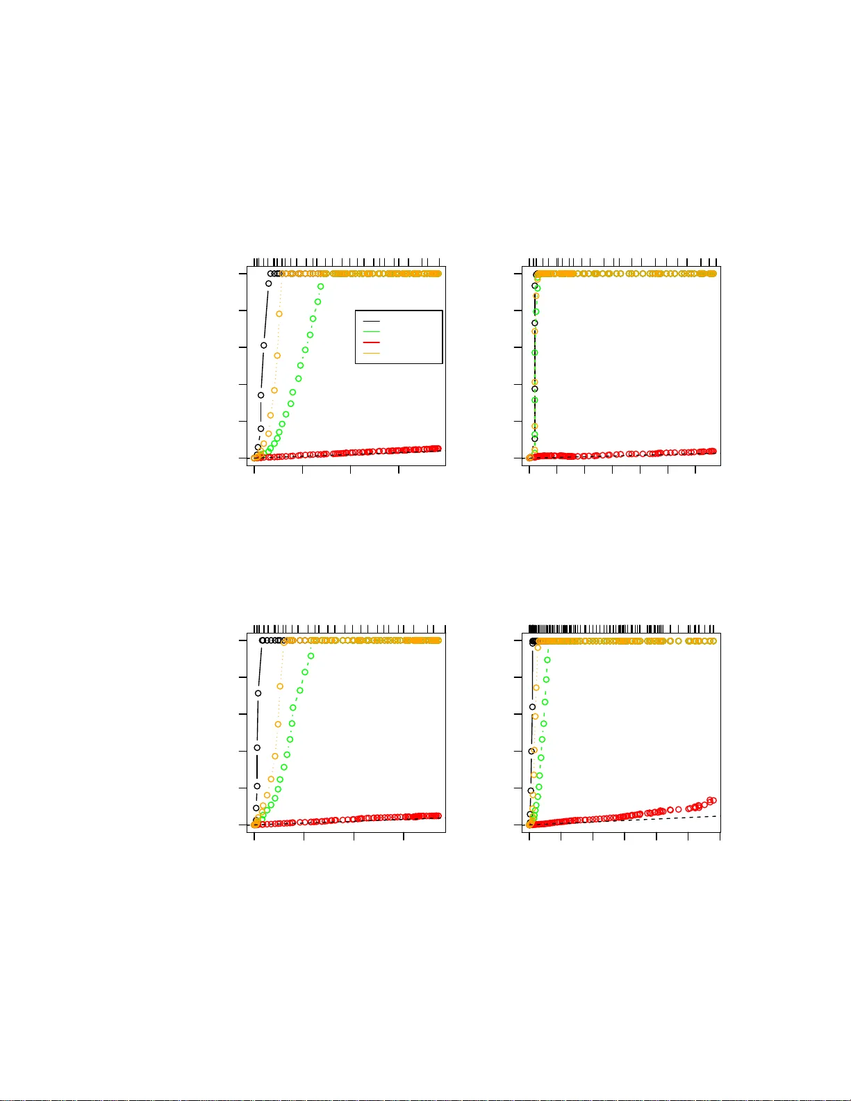
Strong Rules for Discarding Predictors in Lasso -t yp e Problems Rob ert Tibshirani, ∗ Jacob Bien, Jerome F riedman, T rev or Hastie, Noah Simon, Jonathan T a ylor, Ry an Tibshirani No v ember 26, 2024 Abstract W e consider rules for discarding predictors in lasso regression and related problems, for computational efficiency . El Ghaoui et al. (2010) prop ose “SAFE” rules, based on univ ariate inner product s b etw een each predictor and t h e outcome, th at guarantee a co efficient will b e zero in the solutio n vector. This pro vides a reduction in th e num b er of v ariables that need to b e entered into the optimization. In this pap er, we prop ose str ong r ules that are n ot foolpro of b u t rarely fail in practice. These are very simple, and can be complemented with simple chec ks of t h e Karush- Kuhn-T uc ker ( K KT) conditions t o ensure that the exact solution to the conv ex problem is delivered. These rules offer a sub stantia l sa vings in b oth computational time and memory , for a v ariety of statistical optimization problems. 1 In tro d u ction Our focus her e is on statistical mo dels fit using ℓ 1 regular iz ation. W e star t with pena lized linea r r egres s ion. Consider a pro blem with N obser v ations and p predictors, and let y denote the N -vector of outcomes , and X b e the N × p matrix o f pr edictors, with j th co lumn x j and i th row x i . F or a set of indices A = { j 1 , . . . j k } , we write X A to denote the N × k submatrix X A = [ x j 1 , . . . x j k ], and a lso b A = ( b j 1 , . . . b j k ) for a v ector b . W e assume that the pre dic to rs and outcome are cent er ed, so we can omit an intercept term fr om the mo del. The lasso Tibshirani (199 6) solves the optimization problem ˆ β = a rgmin β 1 2 k y − X β k 2 2 + λ k β k 1 , (1) ∗ Departmen ts of Statistics and Health R esearch and P oli cy , Stanford Uni versity , Stanford CA 94305, USA. E-mail: tibs@s tanford. edu 1 where λ ≥ 0 is a tuning parameter. Ther e has b een considera ble work in the past few years deriving fast algor ithms for this problem, esp ecially fo r lar ge v alues o f N and p . A main reason for using the lass o is that the ℓ 1 pena lty tends to g ive exact zeros in ˆ β , a nd therefore it p erfor ms a kind o f v ariable selection. Now supp ose w e knew, a priori to solving (1), that a subset of the v ariables S ⊆ { 1 , . . . p } will hav e zero c o efficients in the solution, that is, ˆ β S = 0. Then we could solve pro blem (1) with the des ig n matrix replaced by X S c , where S c = { 1 , . . . p } \ S , for the rema ining coefficients ˆ β S c . If S is relatively large, then this could result in a substantial computatio nal savings. El Ghaoui et al. (201 0) co ns truct such a set S of “ screened” o r “discar ded” v ariables b y lo oking a t the inner pro ducts | x T j y | , j = 1 , . . . p . The authors use a clever ar gument to derive a sur prising set of rules called “SAFE”, and show that applying these r ules can reduce b oth time and memory in the overall computation. In a r elated work, W u e t al. (2009 ) study ℓ 1 pena lized logistic regres s ion and build a scr eened s et S based on similar inner pro ducts. How ever, their construction do es not guar antee that the v aria bles in S actually hav e zero co efficients in the solutio n, and so after fitting on X S c , the authors check the Karush-K uhn-T uck er (K KT) optimality conditions for violations . In the cas e of v io lations, they weaken their set S , and rep eat this pro cess. Also, F a n & Lv (2008) study the s creening of v ariables based on their inner pro ducts in the lasso and related problems, but not fro m a optimization p oint of view. T he ir screening r ules ma y again set coe fficie nt s to zer o tha t are nonzero in the solution, how ever, the author s argue that under certain situations this can lea d to b e tter per formance in terms of estimation risk . In this pap er, we pro p o se str ong rules for disca rding pr e dic to rs in the lasso and other problems that inv o lve lasso -type penalties . These rules discar d many more v ariables than the SAFE rules, but are not fo olpr o of, b ecaus e they can sometimes exclude v aria bles from the model that have nonze ro co efficients in the solution. Therefor e we rely on KKT co nditions to ensure tha t we are indeed computing the cor rect c o efficients in the end. Our metho d is most effectiv e for so lving pr oblems ov er a gr id of λ v alues, b ecause w e can apply our str o ng rules sequentially down the path, which results in a c onsiderable reduction in computational time. Generally sp eaking, the power of the prop osed rules stems from the fact that: • the s et of disca rded v ariables S tends to be larg e and violations rar ely o ccur in practice, and • the rules ar e very simple and can b e applied to many differ ent pr oblems, including the elastic net, lasso p enalized logistic regr e ssion, and the graph- ical lasso. In fact, the violations of the prop os e d rules ar e so rare, that for a while a group of us were trying to establish that they w ere fo olpr o of. A t the same time, others in our group were lo ok ing for counter-examples [hence the larg e n umber of co- authors!]. After many flaw ed pro ofs, w e finally found some counter-examples to 2 the strong sequential b ound (a lthough not to the basic glo bal bo und). Despite this, the strong sequential b ound turns out to b e extremely useful in practice. Here is the layout of this paper . In Section 2 we review the SAFE rules of El Ghaoui et a l. (20 10) for the lasso. The strong rules are introduced and illustrated in Section 3 fo r this same pro ble m. W e demonstrate that the strong r ules r arely make mistakes in practice, esp ecially when p ≫ N . In Section 4 w e g ive a condition under which the strong rules do no t er roneous ly discard predictors (and hence the K KT conditio ns do not need to be chec ked). W e discuss the elastic net and pena lized logistic r e gressio n in Sections 5 and 6. Stro ng r ules for more general conv ex optimizatio n problems a re given in Section 7, and these are applied to the gra phical lasso. In Section 8 w e discuss how the stro ng sequential rule can b e used to sp eed up the solution o f conv ex optimization pr o blems, while s till delivering the exact a nswer. W e a ls o cov er implementation de ta ils of the strong sequen tial rule in our glmnet algorithm (coo rdinate descent for lasso pena lized generalized linear mo dels). Section 9 contains so me final discussio n. 2 Review of the SAFE rules The basic SAFE rule of El Ghaoui et al. (2010) for the las s o is defined as follo ws: fitting at λ , we discar d predictor j if | x T j y | < λ − k x j k 2 k y k 2 λ max − λ λ max , (2) where λ max = max i | x T i y | is the smallest λ for which all co e fficient s a re zero. The authors derive this b ound b y lo o king at a dual of the las s o problem (1). This is: ˆ θ = arg max θ G ( θ ) = 1 2 k y k 2 2 − 1 2 k y + θ k 2 2 (3) sub ject to | x T j θ | ≤ λ for j = 1 , . . . p. The r elationship b etw een the prima l and dual s o lutions is ˆ θ = X ˆ β − y , and x T j ˆ θ ∈      { + λ } if ˆ β j > 0 {− λ } if ˆ β j < 0 [ − λ, λ ] if ˆ β j = 0 (4) for ea ch j = 1 , . . . p . Here is a sk etch of the argument: first w e find a dual feasible po int of the form θ 0 = s y , ( s is a scalar), and hence γ = G ( s y ) represents a low er b ound for the v alue of G at the so lution. Therefore we can add the constraint G ( θ ) ≥ γ to the dual problem (3) and nothing will b e c ha nged. F or each predictor j , we then find m j = a r gmax θ | x T j θ | sub ject to G ( θ ) ≥ γ . 3 If m j < λ (note the stric t inequality), then cer tainly at the solution | x T j ˆ θ | < λ , which implies that ˆ β j = 0 by (4 ). F ina lly , no ting that s = λ/λ max pro duces a dual feasible p oint and rewr iting the co ndition m j < λ gives the r ule (2). In addition to the basic SAFE b o und, the authors also derive a more compli- cated but somewhat b etter bo und that they call “recur sive SAFE” (RECSAFE). As w e will show, the SAFE rules ha ve the a dv ant a ge that they will nev er discard a predictor when its coe fficient is truly nonzero. How ever, they disca rd far fewer predictors than the strong sequential rule , intro duced in the next section. 3 Strong screening rules 3.1 Basic and strong sequen tial rules Our basic (or global) stro ng rule for the la sso problem (1) dis cards pr edictor j if | x T j y | < 2 λ − λ max , (5) where as b efore λ max = max j | x T j y | . When the pr edictors a re standardized ( k x j k 2 = 1 for each j ), it is not difficult to see that the rig ht hand side of (2) is alwa ys smaller than the right ha nd side of (5), so tha t in this ca se the SAFE rule is alwa ys weak er than the basic strong rule. This follows since λ max ≤ k y k 2 , s o tha t λ − k y k 2 λ max − λ λ max ≤ λ − ( λ max − λ ) = 2 λ − λ max . Figure 1 illustrates the SAFE and basic stro ng r ules in an example. When the predictors a re not s tandardized, the o rdering betw een the tw o bo unds is not a s clear , but the s trong rule still tends to disc ard more v ariables in practice unless the predictor s have wildly different margina l v ariances . While (5) is somew ha t us eful, its sequential version is muc h mor e powerful. Suppo se that w e hav e alr e a dy computed the solution ˆ β ( λ 0 ) at λ 0 , and wish to discard predictors for a fit a t λ < λ 0 . Defining the re sidual r = y − X ˆ β ( λ 0 ), our str ong s e qu en tial ru le disc ards predictor j if | x T j r | < 2 λ − λ 0 . (6) Before giving a detailed motiv ation for these rules, we first demonstrate their utilit y . Figure 2 shows s o me examples of the applica tions o f the SAFE a nd strong rules. There are four scenar ios with v ario us v a lues of N a nd p ; in the first three panels, the X matrix is de ns e, while it is spar se in the b ottom right panel. The p opulation co rrela tio n among the fea tur e is zero, p ositive, negative and zer o in the fo ur panels . Finally , 25% of the co efficients ar e no n-zero, with a standa r d Gaussian distribution. In the plots, w e a re fitting along a path of decrea sing λ v alues and the plots show the n umber of predictor s left after screening at each stage. W e see that the SAFE a nd RECSAFE rules only exclude predictors near the beg inning of the path. T he stro ng rules a r e more effective: 4 0.00 0.05 0.10 0.15 0.20 0.25 −0.2 −0.1 0.0 0.1 0.2 Inner product with residual 1 2 3 4 5 6 7 8 9 10 SAFE bound Basic strong bound SAFE bound Basic strong bound λ Figure 1 : SAFE and b asic str ong b oun ds in an example with 10 pr e dictors, lab el le d at the right. The plot shows the inn er pr o duct of e ach pr e dictor with t he curr ent r esidual, with the pr e dictors in the mo del having maximal inner pr o duct e qual t o ± λ . The dotte d vertic al line is dr awn at λ max ; the br oken vertic al line is dr awn at λ . The str ong rule ke eps only pr e dictor #3, while the SAFE b ound ke eps pr e dictors #8 and #1 as wel l. 5 remark ably , the strong sequential r ule discarded almost all of the predictors that hav e co efficients of zero . There were no v iolations o f any o f rules in any of the four scenarios . It is commo n pra ctice to standar dize the predictors before applying the lasso , so that the p enalty term makes s e nse. This is what was done in the examples of Figure 2 . But in some instances, one might not wan t to sta nda rdize the predictors, and so in Figure 3 we in vestigate the per formance o f the r ule s in this case. In the left panel the p opulatio n v ar ia nce of each pre dicto r is the same; in the right panel it v ar ie s by a factor of 50. W e s ee that in the latter case the SAFE rules outpe r form the basic str o ng rule, but the sequential s trong r ule is still the clear winner. There w er e no violations in any of rules in either panel. 3.2 Motiv ation for the st rong rules W e now give s ome motiv ation for the strong rule (5) and later, the sequential rule (6). W e start with the KKT conditions for the lasso pro blem (1) . These are x T j ( y − X ˆ β ) = λ · s j (7) for j = 1 , . . . p , where s j is a s ubgradient of ˆ β j : s j ∈      { +1 } if ˆ β j > 0 {− 1 } if ˆ β j < 0 [ − 1 , 1] if ˆ β j = 0 . (8) Let c j ( λ ) = x T j { y − X ˆ β ( λ ) } , w her e w e emphasize the dependence on λ . Supp ose in general that we could assume | c ′ j ( λ ) | ≤ 1 , (9) where c ′ j is the deriv ative with resp ect to λ , a nd we igno r e poss ible po ints of non-differentiabilit y . This would allow us to conclude that | c j ( λ max ) − c j ( λ ) | =      Z λ max λ c ′ j ( λ ) dλ      (10) ≤ Z λ max λ | c ′ j ( λ ) | dλ (11) ≤ λ max − λ, and so | c j ( λ max ) | < 2 λ − λ max ⇒ | c j ( λ ) | < λ ⇒ ˆ β j ( λ ) = 0 , the last implication following fro m the K KT conditions, (7) and (8). Then the strong rule (5) follows as ˆ β ( λ max ) = 0, so that | c j ( λ max ) | = | x T j y | . Where do es the slop e condition (9) co me from? The pro duct rule applied to (7) g ives c ′ j ( λ ) = s j ( λ ) + λ · s ′ j ( λ ) , (12) 6 0 50 100 150 0 1000 3000 5000 Number of predictors in model Number of predictors left after filtering 0 0.09 0.23 0.35 0.48 SAFE strong/global strong/seq RECSAFE Dense Nocorr n= 200 p= 5000 0 20 40 60 80 120 0 1000 3000 5000 Number of predictors in model Number of predictors left after filtering 0 0.04 0.16 0.25 0.33 0.4 Dense P os n= 200 p= 5000 0 50 100 150 0 1000 3000 5000 Number of predictors in model Number of predictors left after filtering 0 0.09 0.21 0.3 0.4 0.5 Dense Neg n= 200 p= 5000 0 200 600 1000 0 5000 15000 25000 Number of predictors in model Number of predictors left after filtering 0 0.5 0.79 0.9 0.96 0.98 Sparse Nocorr n= 500 p= 50000 Figure 2: L asso r e gr ession: r esult s of differ ent rules applie d to four differ ent sc enarios. Ther e ar e four sc enarios with various values of N and p ; in the firs t thr e e p anels the X matrix is dense, while it is sp arse in the b ottom right p anel. The p opulation c orr elation among the fe atur e is zer o, p ositive, n e gative and zer o in the four p anels. Final ly, 25% of the c o efficients ar e non-zer o, with a standar d Gaussian distribution. In the plots, we ar e fit ting along a p ath of de cr e asing λ values and the plots show the n umb er of pr e dictors left after scr e ening at e ach stage. A br oken line with unit slop e is adde d for r efer enc e. The pr op ortion of varianc e explaine d by the mo del is s hown along the top of the plot. Ther e wer e no violatio n s of any of the rules in any of the four sc enarios. 7 0 50 100 150 0 1000 2000 3000 4000 5000 Number of predictors in model Number of predictors left after filtering 0 0.29 0.5 0.67 0.82 0.93 0.97 SAFE strong/global strong/seq RECSAFE Equal population variance 0 50 100 150 0 1000 2000 3000 4000 5000 Number of predictors in model Number of predictors left after filtering 0 0.29 0.5 0.67 0.82 0.93 0.97 Unequal population variance Figure 3: L asso r e gr ession: r esults of differ ent rules when the pr e dictors ar e not standar dize d. The sc enario in the left p anel is the same as in the top left p anel of Figur e 2, exc ept that t he fe atur es ar e not s t andar dize d b efor e fitting t he lasso. In t he data gener ation for the right p anel, e ach fe atur e is sc ale d by a r andom factor b etwe en 1 and 50, and again, no s t andar dization is done. 8 and a s | s j ( λ ) | ≤ 1, co ndition (9 ) can b e obtained if we s imply dro p the sec- ond ter m a b ov e. F or an active v ariable, that is ˆ β j ( λ ) 6 = 0, we have s j ( λ ) = sign { ˆ β j ( λ ) } , a nd co ntin uit y of ˆ β j ( λ ) with r esp ect to λ implies s ′ j ( λ ) = 0. But s ′ j ( λ ) 6 = 0 for ina ctive v ariables, and hence the bo und (9) can fail, which makes the strong rule (5) imp erfect. It is from this p o int of view—writing out the KKT conditions, taking a deriv ative with resp ect to λ , and dropping a term— that we deriv e str ong rules for ℓ 1 pena lized log istic regre s sion and more general problems. In the lasso ca se, condition (9) has a mor e concr ete interpretation. F r om Efron et al. (2 004), we k now that each co o rdinate of the so lution ˆ β j ( λ ) is a piecewise linear function of λ , hence so is ea ch inner pro duct c j ( λ ). Therefore c j ( λ ) is differentiable at any λ that is no t a kink, the p oints at which v ar ia bles ent er or leav e the mo del. In b etw een kinks, c o ndition (9) is really just a b ound on the slo p e of c j ( λ ). The idea is tha t if we assume the absolute slo p e of c j ( λ ) is at most 1 , then w e can b ound the a mount that c j ( λ ) changes as we mov e fro m λ max to a v alue λ . Hence if the initia l inner pr o duct c j ( λ max ) starts to o far from the maximal achiev ed inner pr o duct, then it cannot “ c a tch up” in time. An illustration is given in Figure 4. The arg ument for the strong b ound (intuitiv ely , an argument a b out slop es), uses only lo ca l information and so it can be applied to solving (1) on a gr id of λ v alues. Hence by the sa me a r gument as be fore, the slop e assumption (9) leads to the strong sequential rule (6). It is interesting to note tha t | x T j r | < λ (13) is just the KKT c ondition for excluding a v ar ia ble in the solution at λ . The strong sequential bound is λ − ( λ 0 − λ ) and we can think of the extra term λ 0 − λ as a buffer to acco unt for the fact that | x T j r | may increase as we move from λ 0 to λ . Note also that as λ 0 → λ , the stro ng sequential rule b eco mes the KKT condition (13), so that in effect the sequential rule at λ 0 “anticipates” the KKT conditions at λ . In summary , it turns out that the key slop e condition (9) very often holds, but can b e violated for s ho rt stretches, esp ecia lly whe n p ≈ N and for small v alues of λ in the “ov er fit” r egime of a lasso problem. In the next section we provide an example that shows a vio lation of the slop e b o und (9), which break s the strong sequential rule (6). W e also give a condition on the design matrix X under which the b ound (9) is g uaranteed to hold. How ever in s imulations in that section, w e find tha t these violations a re rar e in practice and virtually non-existent when p > > N . 9 0.0 0.2 0.4 0.6 0.8 1.0 0.0 0.2 0.4 0.6 0.8 1.0 λ c j = x T j ( y − X ˆ β ) λ max − λ 1 λ 1 λ max Figure 4 : Il lustr ation of t he slop e b ound (9) le ading to the str ong ru le (6) . The inner pr o duct c j is plotte d in r e d as a function of λ , r est ricte d t o only one pr e dictor for simplicity. The slop e of c j b etwe en λ max and λ 1 is b ounde d in absolute value by 1, so the m ost it c an rise over this interval is λ max − λ 1 . Ther efor e, if it starts b elow λ 1 − ( λ max − λ 1 ) = 2 λ 1 − λ max , it c an not p ossibly r e ach the critic al level by λ 1 . 4 Some analysis of the strong rules 4.1 Violation of the slop e condition Here we demonstra te a c ounter-example o f b o th the slop e bo und (9) and of the strong sequential r ule (6). W e belie ve that a c o unter-example for the basic strong rule (5) can also b e constructed, but we hav e not yet found one. Such an example is somewhat more difficult to construct b ecause it would requir e that the av erage s lop e exceed 1 from λ max to λ , ra ther than exceeding 1 for short stretches of λ v alues. W e to ok N = 50 and p = 30, with the entries of y and X drawn inde- pendently from a standar d normal distribution. Then we cen tere d y and the 10 columns o f X , and s ta ndardized the columns o f X . As Figur e 5 shows, the slop e o f c j ( λ ) = x T j { y − X ˆ β ( λ ) } is c ′ j ( λ ) = − 1 . 58 6 for all λ ∈ [ λ 1 , λ 0 ], where λ 1 = 0 . 024 4, λ 0 = 0 . 0 259, and j = 2. Mor eov er, if we were to use the solution at λ 0 to eliminate predictors for the fit at λ 1 , then we would eliminate the 2nd predictor based on the b ound (6). But this is clearly a problem, bec a use the 2nd predictor enters the mo del at λ 1 . By contin uity , we can ch o ose λ 1 in an int er v al a round 0 . 024 4 and λ 0 in an interv al a round 0 . 025 9, a nd still br eak the strong sequential rule (6). 4.2 A sufficien t condition for the slop e b ound Tibshirani & T aylor (2010 ) pr ov e a general result that c an b e used to g ive the following sufficien t co nditio n for the unit slope bo und (9). Under this condition, bo th basic and strong sequential rules are g uaranteed not to fail. Recall that a matrix A is diago nally dominant if | A ii | ≥ P j 6 = i | A ij | for all i . Their result gives us the following: Theorem 1. S u pp ose that X is N × p , with N ≥ p , and of ful l r ank. If ( X T X ) − 1 is diag onally domina nt , (14) then the slop e b ound (9) holds at al l p oints wher e c j ( λ ) is differ entiable, for j = 1 , . . . p , and henc e the str ong rules (5) , (6) never pr o duc e violations. Pr o of. Tibshirani & T aylor (2010) c onsider a genera lized lass o pro blem argmin β 1 2 k y − X ˆ β k 2 2 + λ k D β k 1 , (15) where D is a gener al m × p p enalty matrix. In the pro of of their “b oundar y lemma”, Lemma 1, they show that if rank( X ) = p a nd D ( X T X ) − 1 D T is di- agonally dominant, then the dual s olution ˆ u ( λ ) corr esp onding to pro blem (15) satisfies | ˆ u j ( λ ) − ˆ u j ( λ 0 ) | ≤ | λ − λ 0 | for any j = 1 , . . . m and λ, λ 0 . By piecewise linear it y of ˆ u j ( λ ), this means that | ˆ u ′ j ( λ ) | ≤ 1 at all λ ex cept the kink p oints. F urthermore, when D = I , problem (15) is simply the la sso, and it turns out that the dual solution ˆ u j ( λ ) is exactly the inner pr o duct c j ( λ ) = x T j { y − X ˆ β ( λ ) } . This prov es the slop e bo und (9) under the condition that ( X T X ) − 1 is diagona lly domina nt. Finally , the kink p oints are countable and hence form a set of Leb esgue mea- sure zero. Therefor e c j ( λ ) is differentiable almost everywhere and the integrals in (10) and (11) make sense. This pr ov es the strong rules (5) and (6). W e note a simila rity b etw een co ndition (14) and the p ositive cone condition used in Efron et al. (2004). It is not hard to see that the p ositive cone condition implies (14), and actually (1 4) is a m uch weaker condition b ecause it do esn’t require lo oking at every p os sible subset o f columns. 11 0.000 0.005 0.010 0.015 0.020 0.025 −0.02 −0.01 0.00 0.01 0.02 λ c j = x T j ( y − X ˆ β ) 2 λ 1 − λ 0 λ 1 λ 0 Figure 5: Ex ample of a violation of the slop e b ound (9) , which br e aks the str ong se quential rule (6 ) . The entries of y and X wer e gener ate d as indep endent, standar d normal r andom variable s with N = 50 and p = 3 0 . (Henc e ther e is no underlying signal.) The lines with slop es ± λ ar e the envelop of maximal inner pr o ducts achieve d by pr e dictors in the mo del for e ach λ . F or clarity we only show a short st r etch of t he solution p ath. The rightmost vertic al line is dr awn at λ 0 , and we ar e c onsidering t he new value λ 1 < λ 0 , the vertic al line t o its left. The horizontal line is the b ound (9) . In the top right p art of the plot, the inner pr o duct p ath for the pr e dictor j = 2 is dr awn in r e d, and st arts b elow the b ound, but enters the mo del at λ 1 . The slop e of t he r e d se gment b etwe en λ 0 and λ 1 exc e e ds 1 in absolute value. A dotte d line with slop e -1 is dr awn b eside the r e d se gment for r efer enc e. 12 A s imple mo del in which dia gonal dominance holds is when the co lumns of X are orthono rmal, b eca use then X T X = I . But the diag onal dominance condition (14) certainly holds o utside of the orthog o nal design case. W e give t wo such examples b e low. • Equi-c orr elation mo del. Supp ose that k x j k 2 = 1 for all j , and x T j x k = r for all j 6 = k . Then the in verse o f X T X is ( X T X ) − 1 = I · 1 1 − r − 1 1 − r  11 T 1 + r ( p − 1)  , where 1 is the vector of all ones. This is diag onally dominant as along as r ≥ 0 . • Haar b asis m o del. Supp ose that the columns of X form a Haar basis, the simplest example b eing X =      1 1 1 . . . 1 1 . . . 1      , ( 1 6) the lower triangular matrix of ones. Then ( X T X ) − 1 is diag o nally domi- nant. This arises, for example, in the one-dimensio na l fused lass o where we solve argmin β 1 2 N X i =1 ( y i − β i ) 2 + λ N X i =2 | β i − β i − 1 | . If we transfo r m this problem to the parameter s α 1 = 1 , α i = β i − β i − 1 for i = 2 , . . . N , then we get a lasso with design X as in (16). 4.3 Connection t o the irrepresen table condition The slop e b ound (9) po ssesses an interesting connection to a concept calle d the “irrepr e sentable c o ndition”. Let us write A as the set of active v ariables at λ , A = { j : ˆ β j ( λ ) 6 = 0 } , and k b k ∞ = max i | b i | for a vector b . Then, using the work of Efro n et al. (2004), we can expres s the slop e condition (9) as k X T A c X A ( X T A X A ) − 1 sign( ˆ β A ) k ∞ ≤ 1 , (17) where by X T A and X T A c , w e really mean ( X A ) T and ( X A c ) T , and the sign is applied element -w is e. On the other hand, a co mmon condition app ear ing in work ab out mo de l selection prop erties of lasso, in b oth the finite-sample a nd asymptotic settings, is the so called “irrepr esentable condition” ? , which is close ly related to the 13 concept of “ mutu a l incoherence” ? . Roughly sp eaking , if β T denotes the no nzero co efficients in the true mo del, then the ir represe ntable condition is that k X T T c X T ( X T T X T ) − 1 sign( β T ) k ∞ ≤ 1 − ǫ (18) for some 0 < ǫ ≤ 1. The co nditions (18 ) a nd (1 7) app ea r extremely similar, but a key difference betw ee n the tw o is that the for mer p e rtains to the true co efficient s that gener- ated the data, while the la tter pe rtains to those found b y the lasso optimization problem. Because T is asso ciated w ith the true mo del, we can put a pro ba bility distribution on it and a probability distribution on sig n( β T ), a nd then show that with high proba bility , c ertain des ig ns X ar e mu tually incoherent (18). F or example, Candes & P la n (2009) supp ose that k is sufficiently small, T is drawn from the uniform distribution on k -sized subs e ts of { 1 , . . . p } , a nd each entry of sign( β T ) is equal to +1 o r − 1 with pro bability 1 / 2, independent of ea ch other. Under this mo del, they show that designs X with max j 6 = k | x T j x k | = O (1 / lo g p ) satisfy the irrepre sentable c o ndition with very high pr obability . Unfortunately the same types of arguments ca nnot b e applied directly to (17). A distribution on T and sign( β T ) induces a different dis tr ibution on A and sign( ˆ β A ), via the lasso optimization pro cedure. Even if the dis tr ibutions of T and sign( β T ) are very simple, the dis tributions of A and sign( ˆ β A ) can b eco me quite complica ted. Still, it does not seem hard to believe that confidence in (1 8) translates to some amount of confidence in (17). Luckily for us, we do not need the slop e b o und (17) to hold exactly or with any sp ecified level of proba bilit y , bec ause we are using it as a computational to ol and can simply revert to c hecking the KKT conditions when it fails. 4.4 A n umerical in vestigation of the st rong sequen tial r ule violations W e gener ated Gaussian data with N = 100, v ar ying v alues of the num b er o f predictors p and pa irwise cor relation 0.5 betw een the pr edictors. One q uarter of the coefficients were non-ze ro, with the indices of the nonzer o pre dic to rs randomly chosen a nd their v a lues equal to ± 2. W e fit the lasso for 80 e q ually spaced v alues of λ from λ max to 0, a nd recorded the num b er of viola tions of the strong sequential rule. Figure 6 shows the n umber o f vio la tions (o ut of p predictors) averaged ov er 10 0 simulations: we plot versus the p erce nt v ariance explained instead o f λ , since the for mer is more mea ningful. Since the vertical axis is the total num b er o f viola tions, we see that v io lations are quite ra re in general never averaging more than 0.3 o ut of p predictors . They are more common near the right end of the path. They also tend to occur when p is fairly close to N . When p ≫ N ( p = 500 or 10 00 here), there were no v io lations. Not surprisingly , then, there were no viola tions in the n umer ical exa mples in this pap er since they all hav e p ≫ N . Lo oking at (13), it sugg e sts that if w e take a finer grid of λ v alues, ther e should be fewer vio lations of the rule. How ever we have not found this to b e 14 0.0 0.2 0.4 0.6 0.8 1.0 0.0 0.1 0.2 0.3 0.4 0.5 P ercent variance explained T otal number of violations p=20 p=50 p=100 p=500 p=1000 Figure 6: T otal numb er of violatio ns (out of p pr e dictors) of the st r ong se quent ial rule, for simulate d data with N = 1 00 and varyi n g values of p . A s e qu en c e of mo dels is fit, with de cr e asing values of λ as we move fr om left to right. The fe atur es ar e unc orr elate d. The r esults ar e aver ages over 100 simulations. 15 true n umerically : the av er age num b er of violations a t each g rid point λ stays ab out the same. 5 Screening rules for the elastic net In the e la stic net we solve the pro blem 1 minimize 1 2 || y − X β || 2 + 1 2 λ 2 || β || 2 + λ 1 || β || 1 (19) Letting X ∗ =  X √ λ 2 · I  ; y ∗ =  y 0  , (20) we can write (19) as minimize 1 2 || y ∗ − X ∗ β || 2 + λ 1 || β || 1 . (21) In this for m we ca n a pply the SAFE rule (2) to o btain a r ule for discar ding predictors. Now | x ∗ j T y ∗ | = | x T j y | , || x ∗ j || = p || x j || 2 + λ 2 , || y ∗ || = || y || . Hence the global rule for discar ding pre dic to r j is | x T j y | < λ 1 − || y || · q || x j || 2 + λ 2 · λ 1 max − λ 1 λ 1 max (22) Note that the glmnet pack ag e uses the parametrization ((1 − α ) λ, αλ ) ra ther than ( λ 2 , λ 1 ). With this parametrizatio n the basic SAFE rule has the form | x T j y | <  αλ − || y || · q || x j || 2 + (1 − α ) λ · λ max − λ λ max  (23) The s trong screening rules turn out to be the sa me as for the lass o . With the glmne t parametr ization the g lobal rule is simply | x T j y | < α (2 λ − λ max ) (24) while the sequential rule is | x T j r | < α (2 λ − λ 0 ) . (25) Figure 7 show results for the elastic net with standard indep endent Gaussian data, n = 1 00 , p = 100 0, for 3 v alues o f α . There were no violations in any o f these figures, i.e. no predictor was discarded that had a non-zero co efficient at the actual solution. Again w e see that the strong sequential r ule per forms extremely well, leaving only a sma ll num b er o f ex cess predictors at each stage. 1 This differs from the original f orm of the “naive” elastic net in Zou & Hastie (2005) by the factors of 1 / 2, just f or notational con venience . 16 0 100 300 500 0 200 400 600 800 1000 Number of predictors in model Number of predictors left after filtering 0 0.4 0.69 0.86 0.97 SAFE strong global strong/seq 0 50 100 150 200 0 200 400 600 800 1000 Number of predictors in model Number of predictors left after filtering 0 0.33 0.7 0.82 0.98 0 40 80 120 0 200 400 600 800 1000 Number of predictors in model Number of predictors left after filtering 0 0.31 0.57 0.87 0.99 α = 0 . 1 α = 0 . 5 α = 0 . 9 Figure 7: Elastic net: results for differ ent rules for thr e e differ ent values of the mixing p ar ameter α . In t he plots, we ar e fi tting along a p ath of de cr e asing λ values and the plots show the n umb er of pr e dictors left after scr e ening at e ach stage. The pr op ortion of varianc e explaine d by the mo del is shown along t he top of the plot is shown. Ther e wer e n o violations of any of the rules in the 3 sc enarios. 17 6 Screening rules for logistic regression Here we hav e a binary resp onse y i = 0 , 1 and we assume the log istic mo de l Pr( Y = 1 | x ) = 1 / (1 + exp( − β 0 − x T β )) (26) Letting p i = P r( Y = 1 | x i ), the p enalized log -likelihoo d is ℓ ( β 0 , β ) = − X i [ y i log p i + (1 − y i ) log(1 − p i )] + λ || β || 1 (27) El Ghaoui et a l. (2 010) derive an exa ct global rule for discar ding predictors, based on the inner products b etw een y a nd each predictor , using the same kind of dua l arg ument as in the Gaussia n case. Here we investigate the ana logue o f the str ong rules (5) a nd (6). The sub- gradient equation for logistic reg ression is X T ( y − p ( β )) = λ · sign( β ) (28) This leads to the global r ule: letting ¯ p = 1 ¯ y , λ max = ma x | x T j ( y − ¯ p ) | , we discard predictor j if | x T j ( y − ¯ p ) | < 2 λ − λ max (29) The s equential version, star ting a t λ 0 , uses p 0 = p ( ˆ β 0 ( λ 0 ) , ˆ β ( λ 0 )): | x T j ( y − p 0 ) | < 2 λ − λ 0 . (30) Figure 8 show the result of v arious rules in an example, the newsg roup do cument classification problem (Lang 1995). W e used the training set cultured from these data b y Ko h et a l. (2 0 07). The r esp onse is binary , and indicates a sub clas s o f to pic s ; the predictor s are binary , and indica te the pres e nce of particular tri-gra m s equences. The pr edictor matrix ha s 0 . 05% nonzero v alues. 2 Results fo r ar e shown for the new glo ba l rule (29) and the new sequential rule (30). W e were unable to compute the lo gistic re g ressio n global SAFE r ule for this example, using our R languag e implemen tation, as this had a very long computation time. But in smaller examples it perfor med m uch like the glo bal SAFE rule in the Gauss ian case. Again we s ee that the strong sequential rule (30), after computing the inner product of the residuals with all predictors at each s ta ge, allows us to discard the v a st ma jority of the predictors before fitting. There were no violatio ns of either r ule in this example. Some appr oaches to p enalized logistic regres sion such as the gl mnet pack age use a weigh ted lea st squar es itera tion within a Newton step. F or these a lg o- rithms, an alterna tive approach to discar ding pre dic to rs would b e to apply one of the Gaussian rules within the weigh ted least squar es itera tion. 2 This dataset is a v ailable as a sav ed R data ob ject at http://w ww-stat.stanfor d .edu/ hastie/glmn et 18 0 20 40 60 80 100 1e+01 1e+03 1e+05 Number of predictors in model Number of predictors left after filtering strong/global strong/seq Newsgr oup data Figure 8 : L o gistic r e gr ession: r esult s for newsgr oup example, using t he n ew glob al rule (29) and the new se quential ru le (30). The br oken black curve is the 45 o line, dr awn on t he lo g sc ale. 19 W u et a l. (2 009) used | x T j ( y − ¯ p ) | to sc r een pr e dictors (SNPs) in genome- wide asso ciatio n s tudies, wher e the n umber o f v ariables can exceed a million. Since they only anticipated mo dels with say k < 1 5 ter ms, they selected a small m ultiple, say 1 0 k , o f SNPs and computed the las s o solution path to k terms. All the screened SNPs could then b e check ed for vio lations to verify that the solution found was global. 7 Strong rules for general p r ob lems Suppo se that we hav e a conv ex problem of the form minimize β h f ( β ) + λ · K X k =1 g ( β j ) i (31) where f and g are conv ex functions, f is differentiable and β = ( β 1 , β 2 , . . . β K ) with ea ch β k being a scalar or vector. Suppos e fur ther that the subgradient equation for this problem has the for m f ′ ( β ) + λ · s k = 0 ; k = 1 , 2 , . . . K (32) where ea ch subgradient v ariable s k satisfies || s k || q ≤ A , and || s k || q = A when the constraint g ( β j ) = 0 is satisfied (here || · || q is a norm). Supp o se that we have t wo v alues λ < λ 0 , and corre sp onding solutio ns ˆ β ( λ ) , ˆ β ( λ 0 ). Then following the same logic a s in Section 3, we can de r ive the general strong rule || f ( ˆ β 0 k d β k ) || q < (1 + A ) λ − Aλ 0 (33) This ca n be a pplied either globally or sequentially . In the lasso regr ession set- ting, it is easy to chec k that this reduce s to the r ule s (5),(6) where A = 1. The rule (33 ) has many p otential applica tio ns. F or example in the graphica l lasso for sparse inv ers e cov aria nce estimation (F r iedman et al. 200 7), we observe N multiv a r iate norma l observ ations of dimensio n p , with mean 0 and cov a riance Σ, with o bserved empirical cov a riance matr ix S . Letting Θ = Σ − 1 , the problem is to maximize the p enalized lo g -likelihoo d log det Θ − tr( S Θ) − λ || Θ || 1 , (34) ov er no n-negative definite matr ices Θ. The p enalty || Θ || 1 sums the abs olute v alues of the entries of Θ; we a ssume that the diagonal is no t p ena lized. The subgradient equation is Σ − S − λ · Γ = 0 , (35) where Γ ij ∈ sign(Θ ij ). One could apply the rule (33) element wise , a nd this would be use ful for an optimizatio n metho d that op era tes element wise. This gives a rule of the form | S ij − ˆ Σ( λ 0 ) | < 2 λ − λ 0 . How ever, the gra phical lass o algorithm procee ds in a blo ckwise fashion, optimizing one who le ro w and co lumn 20 0 50 100 150 200 250 300 0 50 100 150 200 250 300 Number rows/cols in model Number rows/cols left after filtering strong global strong/seq Figure 9 : S tr ong glob al and se quential rules applie d t o the gr aphic al lasso. A br oken line with unit slop e is adde d for re fer enc e. at a time. Hence for the gra phica l las s o, it is more effectiv e to disca rd en tire rows a nd columns at once. F o r each row i , let s 12 , σ 12 , a nd Γ 12 denote S i, − i , Σ i, − i , and Γ i, − i , resp ectively . Then the subgr adient e quation for one row ha s the form σ 12 − s 12 − λ · Γ 12 = 0 , (36) Now given tw o v alues λ < λ 0 , a nd solution ˆ Σ 0 at λ 0 , we form the sequential rule max | ˆ σ 0 12 − s 12 | < 2 λ − λ 0 . ( 3 7) If this rule is satisfied, we discar d the entire i th row and column o f Θ, and hence set them to zero (but retain the i th diag onal element). Figure 9 shows an example with N = 100 , p = 300 , standa rd indep endent Gaussia n v ariates. No violations of the rule o ccurr ed. Finally , we note that stro ng rules can b e derived in a similar way , for o ther problems suc h as the group lasso (Y uan & Lin 20 07). In particular, if X ℓ denotes the n × p ℓ blo ck of the design matrix cor resp onding to the features in the ℓ th group, then the strong sequential r ule is simply || X T ℓ r || 2 < 2 λ − λ max . When this holds, we set β ℓ = 0 . 21 8 Implemen tation and n umerical studies The strong sequential rule (6) can b e used to provide p otential sp eed improve- men ts in conv ex optimization problems. Generically , given a solution ˆ β ( λ 0 ) and considering a new v alue λ < λ 0 , let S ( λ ) be the indices o f the pr edictors that survive the scre ening rule (6): w e ca ll this the stro ng set . Denote by E the eligible set of predictors. Then a useful strategy would b e 1. Set E = S ( λ ). 2. Solve the pr oblem at v alue λ using only the predictor s in E . 3. Check the KKT conditions at this s olution for all pr edictors. If ther e are no violatio ns, we ar e done. Otherwise add the pr edictors that violate the KKT conditions to the set E , a nd r ep eat steps (b) a nd (c). Depending on how the optimization is done in s tep (b), this can b e quite ef- fective. Now in the g lmnet pro cedure, coo rdinate descen t is used, with w ar m starts ov er a grid of decrea sing v alues of λ . In addition, an “ever-active” set of pr edictors A ( λ ) is maintained, consisting of the indices of all predictors that hav e a non-zero co efficient for some λ ′ greater than the current v alue λ under consideratio n. The solution is first fo und for this active set: then the K KT conditions ar e c heck ed for all predictor s. if there ar e no vio la tions, then we ha ve the solution at λ ; other wise we add the vio la tors into the active set and rep eat. The tw o strategies ab ov e are very simila r, with one using the s tr ong set S ( λ ) and the other using the ever-activ e set A ( λ ). Figur e 10 shows the activ e and strong sets for an example. Althoug h the str ong r ule greatly r educes the total num be r of predictors, it contains more pr edictors than the ever-active set; according ly , vio lations o ccur more often in the ev er - active set than the stro ng set. This effect is due to the high c orrela tion betw een fea tur es and the fact that the signa l v aria bles hav e co efficients of the same sign. It also o ccurs with logistic regr ession with low er corr elations, say 0.2. In ligh t of this, we find that using both A ( λ ) and S ( λ ) can be adv antageous. F or glmn et we adopt the following combined strategy: 1. Set E = A ( λ ). 2. Solve the pr oblem at v alue λ using only the predictor s in E . 3. Check the KKT c o nditions at this solution for all predictor s in S ( λ ). If there are violations, add these predictor s int o E , and g o back to step (a) using the curr ent solution a s a warm start. 4. Check the K KT co nditions for all predictors. If there are no viola tions, we are do ne . Other wise add these violator s into A ( λ ), reco mpute S ( λ ) and go back to step (a) using the cur r ent solution as a warm star t. Note that viola tions in s tep (c) ar e fa ir ly common, while those in s tep (d) ar e rare. Hence the fac t that the size of S ( λ ) is ≪ p can make this a n e ffective strategy . 22 0 20 40 60 80 0 5000 15000 Number of predictors in model Number of predictors ev er active strong/seq 0 20 40 60 80 0 200 600 1000 Number of predictors in model Number of predictors Figure 10: Gaussian lasso setting, N = 2 00 , p = 20 , 000 , p airwise c orr elation b etwe en fe atur es of 0 . 7 . The first 50 pr e dictors have p ositive, de cr e asing c o- efficients. Shown ar e the nu mb er of pr e dictors left after applying the str ong se quential ru le (6) and t he numb er that have ever b e en active (i.e. had a non- zer o c o efficient in t he solution) for values of λ lar ger than the curr ent value. A br oken line with un it slop e is adde d for r efer enc e. The right-hand plot is a zo ome d version of the left plot. 23 W e implemen ted this stra tegy and compare it to the standard glm net alg o- rithm in a v ariety of problems, shown in T ables 1–3. Details are given in the table captions. W e see that the new strategy offers a sp eedup factor of five or more in some cases, and never seems to s low things down. The strong sequential rules a lso ha ve the p o tential for space savings. With a large dataset, o ne could compute the inner products { x T j r } p 1 offline to determine the strong set of predictors, and then carry out the in tensive optimization s teps in memory using just this subset of the pr edictors. 9 Discussion In this pap er w e hav e pro p osed strong global and sequen tial rules for discarding predictors in statistical conv ex optimization problems such as the lasso. When combined with chec ks of the K KT co nditions, these ca n offer substa ntial im- prov ements in sp eed while still yielding the exac t solution. W e pla n to include these rules in a future version of the g lmnet pa ck ag e . The RECSAFE method uses the solution at a g iven point λ 0 to derive a rule for discarding predicto r s at λ < λ 0 . Here is ano ther wa y to (p otentially) a pply the SAFE rule in a sequential manner. Supp os e that we have ˆ β 0 = ˆ β ( λ 0 ), and r = y − X ˆ β 0 , and we consider the fit at λ < λ 0 , with r = y − X ˆ β 0 . Defining λ 0 = max j ( | x T j r | ); (38) we discard predictor j if | x T j r | < λ − || r ||| x j || λ 0 − λ λ 0 (39) W e hav e been unable to prove the correctness o f this rule, and do not know if it is infallible. At the same time, we have b een no t b een able to find a numerical example in which it fails. Ac kno wle dgements: W e thank Stephen Bo yd for his comments, and Lau- rent El Ghaoui and his co- authors for sharing their pap er with us b efor e publi- cation, and fo r helpful feedback o n their work. The first a uthor was supp orted by National Science F oundation Grant DMS-9971 405 and National Institutes of Health Contract N01-HV-28 183. References Candes, E. J. & Plan, Y . (2009), ‘Near-ideal mo del selection by ℓ 1 minimization’, Annals of Statistics 37 (5), 214 5–21 77. Efron, B., Hastie, T., Johnstone, I. & Tibshirani, R. (2004), ‘Least a ng le regr es- sion’, Annals of Statistics 32 (2), 407 –499 . 24 El Ghaoui, L., Viallon, V. & Ra bba ni, T. (201 0), Safe featur e elimination in sparse sup erv ised learning, T echnical Repo rt UC/E E CS-201 0-126 , EE CS Dept., Universit y of California at Ber keley . F an, J . & Lv, J . (2008), ‘Sure indep e ndence scr eening for ultra-high dimensional feature space’, Journ al of the Roy al Statistic al So ciety Series B, to app e ar . F riedman, J., Hastie, T., Ho efling, H. & Tibshira ni, R. (200 7), ‘Path wise co o r- dinate optimization’, Annals of Applie d Statistics 2 (1), 302 – 332. F uchs, J. (2005), ‘Recov er y of ex act spar se represe nt a tions in the presense of noise’, IEEE T r ansactions on Information The ory 51 (10), 36 01–3 6 08. Koh, K ., K im, S.-J. & Boyd, S. (2007), ‘An interior-p oint method for large-sca le l1-regula rized logistic reg ression’, J ournal of Machine L e arning R ese ar ch 8 , 1519– 1 555. Lang, K . (1995 ), Newsweeder: Lear ning to filter netnews., in ‘Pro ceeding s of the Twen ty-First International Co nference o n Machine Lear ning (ICML)’, pp. 331– 339. Meinhausen, N. & Buhlma nn, P . (2006), ‘High-dimensional graphs and v ar ia ble selection with the lasso ’, Annals of Statistics 3 4 , 1436– 1 462. Tibshirani, R. (19 9 6), ‘Regressio n shrink a g e and selection via the lasso’, Journal of the R oyal St atistic al So ciety Series B 58 (1 ), 26 7–288 . Tibshirani, R. & T aylor, J . (2010), The so lution path of the generalized lasso. Submitted. * http ://ww w- stat.stanford.edu/ ~ ryanti bs/pa pers/ genlasso.pdf T ropp, J. (200 6), ‘Jus t rela x: Conv ex progr a mming metho ds for identify- ing spar se signals in nois e’, IEEE T r ansactions on Information The ory 3 (52), 1030 – 1051 . W ainwrigh t, M. (2006), Shar p thre sholds for high-dimensiona l and noisy spar- sity recovery using ℓ 1 -constrained quadr atic pro g ramming (lasso), T echni- cal r ep ort, Statistics a nd EECS Depts., Univ ers ity of Ca lifornia at Berkeley . W u, T. T., Chen, Y. F., Hastie, T., Sobel, E . & Lange, K. (2009), ‘Geno mewide asso cia tio n ana lysis by la s so p enalized logistic regre ssion’, Bioinforma t ics 25 (6), 714–7 21. Y uan, M. & Lin, Y. (20 07), ‘Mo del selection and estimation in regr ession with gr oup ed v ariables’, J ournal of t he Roy al St atistic al So ciety, Series B 68 (1), 49–67 . Zhao, P . & Y u, B. (2006 ), ‘On mo del selection consistency of the las so’, Journal of Machine L e arning R ese ar ch 7 , 2541 –256 3 . 25 Zou, H. & Hastie, T . (2005), ‘Regularization and v ar ia ble selection via the elastic net’, Journal of t he R oyal Statistic al S o ciety Series B. 67 (2), 3 01–3 20. 26 T able 1 : Glmnet timings (se c onds) for fitting a lasso pr oblem in t he Gaussian setting. In the first four c olumns, ther e ar e p = 1 00 , 00 0 pr e dictors, N = 200 observations, 30 n onzer o c o efficie n ts, with the same value and signs alternat- ing; signal-to-noise r atio e qual to 3. In the rightmost c olumn, the data matrix is sp arse, c onsisting of just zer os and ones, with 0 . 1% of the values e qual to 1. Ther e ar e p = 50 , 00 0 pr e dictors, N = 500 observations, with 25% of the c o efficients nonzer o, having a Gaussian distribution; signal-to-noise r atio e qual to 4.3. Metho d Population corr e la tion 0.0 0.25 0.5 0.7 5 Sparse glmnet 4.07 6.1 3 9.50 17.70 4.14 with seq- strong 2.50 2.5 4 2.62 2.98 2.5 2 T able 2 : Glmnet timings (se c onds) for fit ting an elastic n et pr oblem. Ther e ar e p = 100 , 000 pr e dictors, N = 2 00 observations, 30 nonzer o c o efficients, with t he same value and signs alternating; signal-to-noise r atio e qual to 3 Metho d α 1.0 0.5 0.2 0.1 0.01 glmnet 9.49 7.9 8 5.88 5.34 5.2 6 with seq-stro ng 2.64 2.6 5 2.73 2.99 5.44 T able 3: Glmnet timings (se c onds) fitting a lasso/lo gistic r e gr ession pr oblem. Her e the data matrix is sp arse, c onsisting of just zer os and ones, with 0 . 1% of the values e qual to 1. Ther e ar e p = 5 0 , 000 pr e dictors, N = 800 observations, with 30% of the c o efficients nonzer o, with the same value and signs alternating; Bayes err or e qual to 3%. Metho d Population cor relation 0.0 0.5 0.8 glmnet 11.71 12.4 1 12.69 with seq-stro ng 6.31 9 .491 12 .86 27