Learning Planar Ising Models

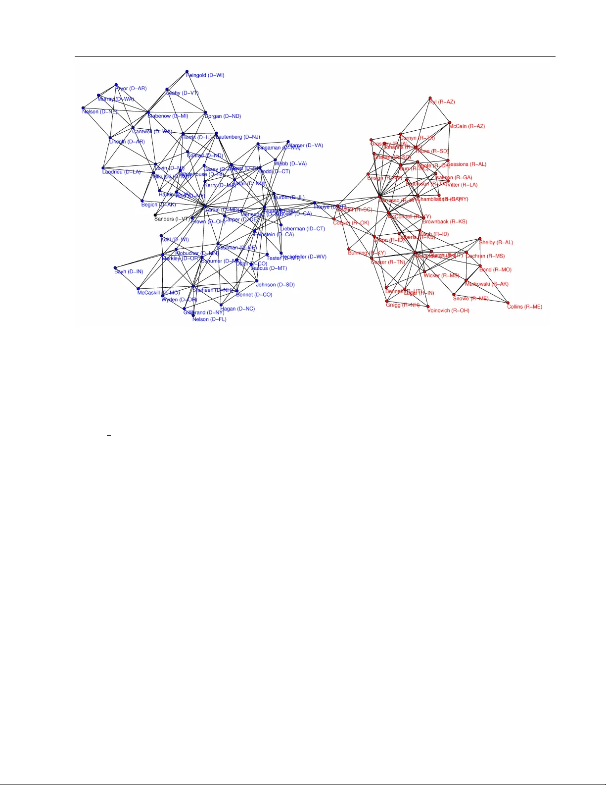
Learning Planar Ising Mo dels Jason K. Johnson Praneeth Netrapalli Mic hael Chertk o v Cen ter for Nonlinear Studies & Theoretical Division T-4 Los Alamos National Laboratory , Los Alamos NM Departmen t of Electrical and Computer Engineering The Univ ersit y of T exas at Austin, Austin TX Cen ter for Nonlinear Studies & Theoretical Division T-4 Los Alamos National Lab oratory , Los Alamos NM Abstract Inference and learning of graphical mo dels are b oth w ell-studied problems in statistics and machine learning that ha v e found man y applications in science and engineering. How- ev er, exact inference is intractable in gen- eral graphical mo dels, whic h suggests the problem of seeking the b est appro ximation to a collection of random v ariables within some tractable family of graphical mo dels. In this pap er, w e focus our atten tion on the class of planar Ising mo dels, for which in- ference is tractable using tec hniques of sta- tistical physics [Kac and W ard; Kasteleyn]. Based on these techniques and recent meth- o ds for planarity testing and planar embed- ding [Chrobak and P ayne], w e propose a sim- ple greedy algorithm for learning the best planar Ising mo del to appro ximate an arbi- trary collection of binary random v ariables (p ossibly from sample data). Giv en the set of all pairwise correlations among v ariables, w e select a planar graph and optimal pla- nar Ising model defined on this graph to b est appro ximate that set of correlations. W e demonstrate our metho d in some sim ulations and for the application of mo deling senate v oting records. 1 In tro duction Graphical mo dels [Lau96, Mac03] are widely used to represen t the statistical relations among a set of ran- dom v ariables. No des of the graph corresp ond to ran- dom v ariables and edges of the graph represent statis- tical in teractions among the v ariables. The problems of inference and learning on graphical mo dels are en- coun tered in many practical applications. The prob- lem of inference is to deduce certain statistical prop er- ties (suc h as marginal probabilities, mo des etc.) of a giv en set of random v ariables whose graphical mo del is kno wn. It has wide applications in areas such as error correcting co des, statistical physics and so on. The problem of learning on the other hand is to deduce the graphical mo del of a set of random v ariables given statistics (p ossibly from samples) of the random v ari- ables. Learning is also a widely encoun tered problem in areas such as biology , anthropology and so on. A certain class of binary-v ariable graphical mo dels with pairwise interactions known as the Ising mo del has b een studied b y physicists as a simple mo del of order-disorder transitions in magnetic materials [Ons44]. Remark ably , it was found that in the sp ecial case of an Ising mo del with zero-mean {− 1 , +1 } binary random v ariables and pairwise interactions defined on a planar graph, calculation of the partition function (whic h is closely tied to inference) is tractable, essen- tially reducing to calculation of a matrix determinan t ([KW52, She60, Kas63, Fis66]). These metho ds ha v e recen tly found uses in machine learning [SK08, GJ07]. In this pap er, w e address the problem of approximat- ing a collection of binary random v ariables (giv en their pairwise marginal distributions) b y a zero-mean planar Ising model. W e also consider the related problem of selecting a non-zero mean Ising mo del defined on an outer-planar graph (these mo dels are also tractable, b eing essentially equiv alen t to a zero-field mo del on a related planar graph). There has b een a great deal of w ork on learning graph- ical models. Muc h of these has fo cused on learning o ver the class of thin graphical models [BJ01, KS01, SCG09] for which inference is tractable b y con vert- ing the model to tree-structured model. The sim- plest case of this is learning tree mo dels (treewidth Learning Planar Ising Mo dels one graphs) for which it is tractable to find the best tree model by reduction to a max-weigh t spanning tree problem [CL68]. Ho wev er, the problem of find- ing the b est b ounded-treewidth mo del is NP-hard for treewidths greater than t w o [KS01], and so heuris- tic metho ds are used to select the graph structure. One popular method is to use con vex optimization of the log-likelihoo d p enalized b y ` 1 norm of param- eters of the graphical mo del so as to promote spar- sit y [BEd08, LGK06]. T o go beyond low treewidth graphs, suc h metho ds either fo cus on Gaussian graph- ical mo dels or adopt a tractable approximation of the lik eliho od. Other metho ds seek only to learn the graph structure itself [R WL10, AKN06] and are often able to demonstrate asymptotic correctness of this estimate under appropriate conditions. One useful application of learning Ising mo dels is for modeling interactions among neurons [CLM07]. The rest of the pap er is organized as follo ws: W e presen t the requisite mathematical preliminaries in Section 2. Section 3 con tains our algorithm along with estimates of its computational complexit y . W e presen t sim ulation results in Section 4 and an application to the senate voting record in Section 5. W e conclude in Section 5 and suggest promising directions for further researc h and dev elopment. All the proofs of prop osi- tions are delegated to an app endix. 2 Preliminaries In this section, w e dev elop our notation and briefly review the necessary bac kground theory . W e will b e dealing with binary random v ariables throughout the pap er. W e write P ( x ) to denote the probabil- it y distribution of a collection of random v ariables x = ( x 1 , . . . , x n ). Unless otherwise stated, we work with undirected graphs G = ( V , E ) with vertex (or no de) set V and edges { i, j } ∈ E ⊂  V 2  . F or ver- tices i, j ∈ V we write G + ij to denote the graph ( V , E ∪ { i, j } ). A (p airwise) gr aphic al mo del is a probability distribu- tion P ( x ) = P ( x 1 , . . . , x n ) that is defined on a graph G = ( V , E ) with vertices V = { 1 , .., n } as P ( x ) ∝ Y i ∈ V ψ i ( x i ) Y { i,j }∈ E ψ ij ( x i , x j ) ∝ exp { X i ∈ V f i ( x i ) + X { i,j }∈ E f ij ( x i , x j ) } (1) where ψ i , ψ ij ≥ 0 are non-negativ e no de and edge com- patibilit y functions. F or p ositiv e ψ ’s, w e may also rep- resen t P ( x ) as a Gibbs distribution with potentials f i = log ψ i and f ij = log ψ ij . 2.1 En trop y , Div ergence and Lik eliho od F or an y probability distribution P on some sample space χ , its entr opy is defined as [CT06] H ( P ) = − X x ∈ χ P ( x ) log P ( x ) Supp ose w e wan t to calculate how well a probability distribution Q approximates another probability dis- tribution P (on the same sample space χ ). F or any t wo probabilit y distributions P and Q on some sample space χ , w e denote b y D ( P, Q ) the Kul lb ack-L eibler diver genc e (or r elative entr opy ) b et w een P and Q . D ( P, Q ) = X x ∈ χ P ( x ) log P ( x ) Q ( x ) The lo g-likeliho o d function is defined as follo ws: LL ( P , Q ) = X x ∈ χ P ( x ) log Q ( x ) The probabilit y distribution in a family F that max- imizes the log-lik eliho od of a probability distribution P is called the maximum-likeliho o d estimate of P in F , and this is equiv alen t to the minimum-diver genc e pr oje ction of P to F : P F = arg max Q ∈F LL ( P , Q ) = arg min Q ∈F D ( P, Q ) 2.2 Exponential F amilies A set of random v ariables x = ( x 1 , . . . , x n ) are said to b elong to an exp onential family [BN79, WJ08] if there exist functions φ 1 , · · · , φ m (the fe atur es of the family) and scalars ( p ar ameters ) θ 1 , · · · , θ m suc h that the join t probabilit y distribution on the v ariables is given by P ( x ) = 1 Z ( θ ) exp X α θ α φ α ( x ) ! where Z ( θ ) is a normalizing constant called the p arti- tion function . This corresp onds to a graphical mo del if φ α happ en to b e functions on small subsets (e.g., pairs) of all the n v ariables. The graph corresp onding to such a probability distribution is the graph where t wo no des hav e an edge b et ween them if and only if there exists α such that φ α dep ends on both v ariables. If the functions { φ α } are non-degenerate (please refer to [WJ08] for details), then for an y ac hiev able momen t parameters µ = E P [ φ ] (for an arbitrary distribution P ) there exists a unique parameter vector θ ( µ ) that realizes these moments within the exp onen tial family . Let Φ( θ ) denote the lo g-p artition function Φ( θ ) , log Z ( θ ) Jason K. Johnson, Praneeth Netrapalli, Mic hael Chertko v F or an exp onen tial family , w e hav e the following im- p ortan t relation (of c onjugate duality ) b et w een the log- partition function and negativ e entrop y of the corre- sp onding probability distribution H ( µ ) , H ( P θ ( µ ) ) as follo ws [WJ08] Φ ∗ ( µ ) , max θ ∈ R m  µ T θ − Φ( θ )  = − H ( µ ) (2) if the mean parameters µ are achiev able under some probabilit y distribution. In fact, this corresp onds to the problem of maximizing the log-lik elihoo d rel- ativ e to an arbitrary distribution P with momen ts µ = E P [ φ ] ov er the exponential family . The optimal c hoice of θ realizes the given momen ts ( E θ [ φ ] = µ ) and this solution is unique for non-degenerate choice of features. 2.3 Ising Graphical Model The Ising mo del is a famous mo del in statistical ph ysics that has b een used as simple model of mag- netic phenomena and of phase transitions in complex systems. Definition 1. An Ising model on binary r andom vari- ables x = ( x 1 , . . . , x n ) and gr aph G = ( V , E ) is the pr ob ability distribution define d by P ( x ) = 1 Z ( θ ) exp   X i ∈ V θ i x i + X { i,j }∈ E θ ij x i x j   wher e x i ∈ {− 1 , 1 } . Thus, the mo del is sp e cifie d by vertex p ar ameters θ i and e dge p ar ameter θ ij . This defines an exp onen tial family with non- degenerate features ( φ i ( x ) = x i , i ∈ V ) and ( φ ij ( x ) = x i x j , { i, j } ∈ E ) and with corresp onding moments ( µ i = E [ x i ] , i ∈ V ) and ( µ ij = E [ x i x j ] , { i, j } ∈ E ). In fact, any graphical mo del with binary v ariables and soft pairwise p oten tials can b e represented as an Ising mo del with binary v ariables x i = {− 1 , +1 } and with parameters θ i = 1 2 X x i x i f i ( x i ) + 1 4 X { i,j }∈ E X x i ,x j x i f ij ( x i , x j ) θ ij = 1 4 X x i ,x j x i x j f ij ( x i , x j ) . There is also a simple corresp ondence b et w een the mo- men t parameters of the Ising mo del and the no de and edge-wise marginal distributions. Of course, it is triv- ial to compute the moments giv en these marginals: µ i = P x i x i P ( x i ) and µ ij = P x i ,x j x i x j P ( x i , x j ). The marginals are recov ered from the moments b y: P ( x i ) = 1 2 (1 + µ i x i ) P ( x i , x j ) = 1 4 (1 + µ i x i + µ j x j + µ ij x i x j ) W e will b e esp ecially concerned with the follo wing sub- family of Ising mo dels: Definition 2. A n Ising mo del is said to b e zero-field if θ i = 0 for al l i ∈ V . It is zero-mean if µ i = 0 ( P ( x i = ± 1) = 1 2 ) for al l i ∈ V . It is simple to v erify that the Ising mo del is zero-field if and only if it is zero-mean. Although the assump- tion of zero-field app ears very restrictive, a general Ising mo del can b e represented as a zero-field model by adding one auxiliary v ariable no de connected to ev ery other node of the graph [GJ07]. The parameters and momen ts of the tw o models are then related as follo ws: Prop osition 1. Consider the Ising mo del on G = ( V , E ) with V = { 1 , . . . , n } , p ar ameters { θ i } and { θ ij } , moments { µ i } and { µ ij } and p artition function Z . L et b G = ( b V , b E ) denote the extende d gr aph b ase d on no des b V = V ∪ { n + 1 } with e dges b E = E ∪ {{ i, n + 1 } , i ∈ V } ) . We define a zer o-field Ising mo del on b G with p ar am- eters { b θ ij } , moments { b µ ij } and p artition function b Z . If we set the p ar ameters ac c or ding to b θ ij =  θ i if j = n + 1 θ ij otherwise then b Z = 2 Z and b µ ij =  µ i if j = n + 1 µ ij otherwise Th us, inference on the corresp onding zero-field Ising mo del on the extended graph b G is essentially equiv- alen t to inference on the (non-zero-field) Ising mo del defined on G . 2.4 Inference for Planar Ising Models The motiv ation for our pap er is the follo wing result on tractabilit y of inference for the planar zer o-field Ising mo del . Definition 3. A gr aph is planar if it may b e emb e dde d in the plane without any e dge cr ossings. Moreo ver, it is kno wn that an y planar graph can b e em b edded suc h that all edges are drawn as straigh t lines. Theorem 1. [KW52][She60] L et Z denote the p ar- tition function of a zer o-field Ising mo del define d on a planar gr aph G = ( V , E ) . L et G b e emb e dde d in the plane (with e dges dr awn as str aight lines) and let φ ij k ∈ [ − π, + π ] denote the angular differ enc e (turn- ing angle) b etwe en dir e cte d e dges ( i, j ) and ( j, k ) . We define the matrix W ∈ C 2 | E |× 2 | E | indexe d by dir e cte d Learning Planar Ising Mo dels e dges of the gr aph as fol lows: W = AD wher e D is the diagonal matrix with D ij,ij = tanh θ ij , w ij and A ij,kl =  exp( 1 2 √ − 1 φ ij l ) , j = k and i 6 = l 0 , otherwise Then, the p artition function of the zer o-field planar Ising mo del is given by: Z = 2 n   Y { i,j }∈ E cosh θ ij   det( I − W ) 1 2 W e briefly remark the combinatorial in terpretation of this theorem: W is the generating matrix of non- rev ersing w alks of the graph with the weigh t of a walk γ b eing w γ = Y ( i,j ) ∈ γ w ij Y ( i,j,k ) ∈ γ exp( 1 2 √ − 1 φ ij k ) . The determinant can be interpreted as the (inv erse) graph zeta function: det( I − W ) = Q γ (1 − w γ ) where the product is taken ov er all equiv alence classes of ape- rio dic closed non-rev ersing w alks [She60, Lo e10]. A related metho d for computing the Ising mo del parti- tion function is based on coun ting p erfect matc hing of planar graphs [Kas63, Fis66]. W e fav or the Kac-W ard approac h only b ecause it is somewhat more direct. Since calculation of the partition function reduces to calculating the determinan t of a matrix, one may use standard Gaussian elimination metho ds to ev al- uate this determinant with complexity O ( n 3 ). In fact, using the generalized nested dissection algo- rithm to exploit sparsit y of the matrix, the complex- it y of these calculations can be reduced to O ( n 3 / 2 ) [LR T79, L T79, GL V00]. Th us, inference of the zero- field planar Ising mo del is tractable and scales w ell with problem size. It also turns out that the gradient and Hessian of the log-partition function Φ( θ ) = log Z ( θ ) can b e calcu- lated efficiently from the Kac-W ard determinant for- m ula. W e recall that deriv atives of Φ( θ ) reco v er the momen t parameters of the exp onential family mo del [BN79, WJ08]: ∇ Φ( θ ) = E θ [ φ ] = µ. Th us, inference of momen ts (and node and edge marginals) are likewise tractable for the zero-field pla- nar Ising mo del. Prop osition 2. L et µ = ∇ Φ( θ ) , H = ∇ 2 Φ( θ ) . L et S = ( I − W ) − 1 A and T = ( I + P )( S ◦ S T )( I + P T ) wher e A and W ar e define d as in The or em 1, ◦ denotes the element-wise pr o duct and P is the p ermutation ma- trix swapping indic es of dir e cte d e dges ( i, j ) and ( j , i ) . Then, µ ij = w ij − 1 2 (1 − w 2 ij )( S ij,ij + S j i,j i ) H ij,kl =  1 − µ 2 ij if ij = k l, else − 1 2 (1 − w 2 ij ) T ij,kl (1 − w 2 kl ) Note, calculating the full matrix S requires O ( n 3 ) cal- culations. Ho w ev er, to compute just the moments µ only the diagonal elements of S are needed. Then, using the generalized nested dissection metho d, infer- ence of moments (edge-wise marginals) of the zero-field Ising model can b e ac hiev ed with complexit y O ( n 3 / 2 ). Ho wev er, computing the full Hessian is more exp en- siv e, requiring O ( n 3 ) calculations. Inference for Outer-Planar Graphical Mo dels W e emphasize that the ab o ve calculations require b oth a planar graph G and a zero-field Ising mo del. Us- ing the graphical transformation of Prop osition 1, the latter zero-field condition may be relaxed but at the exp ense of adding an auxiliary no de connected to all the other no des. In general planar graphs G , the new graph b G may not b e planar and hence may not admit tractable inference calculations. Ho w ev er, for the sub- set of planar graphs where this transformation does preserv e planarit y inference is still tractable. Definition 4. A gr aph G is said to b e outer-planar if ther e exists an emb e dding of G in the plane wher e al l the no des ar e on the outer fac e. In other words, the graph G is outer-planar if the ex- tended graph b G (defined b y Proposition 1) is planar. Then, from Prop osition 1 and Theorem 1 it follows that: Prop osition 3. [GJ07] The p artition function and moments of any outer-planar Ising gr aphic al mo del (not ne c essarily zer o-field) c an b e c alculate d efficiently. Henc e, infer enc e is tr actable for any binary-variable gr aphic al mo del with p airwise inter actions define d on an outer-planar gr aph. This motiv ates the problem of learning outer-planar graphical mo dels for a collection of (p ossibly non-zero mean) binary random v ariables. 3 Learning Planar Ising Mo dels This section addresses the main goals of the pap er, whic h are tw o-fold: 1. Solving for the maximum-lik eliho o d Ising mo del on a given planar graph to b est approximate a collection of zero-mean random v ariables. Jason K. Johnson, Praneeth Netrapalli, Mic hael Chertko v 2. How to select (heuristically) the planar graph to obtain the b est appro ximation. W e address these resp ectiv e problems in the follow- ing t w o subsections. The solution of the first prob- lem is an in tegral part of our approach to the sec- ond. Both solutions are easily adapted to the context of learning outer-planar graphical mo dels of (possibly non-zero mean) binary random v ariables. 3.1 ML P arameter Estimation As discussed in Section 2.2, maximum-lik elihoo d es- timation o v er an exp onential family is a conv ex opti- mization problem (2) based on the log-partition func- tion Φ( θ ). In the case of the zero-field Ising mo del de- fined on a giv en planar graph it is tractable to compute Φ( θ ) via a matrix determinant describ ed in Theorem 1. Th us, w e obtain an unconstrained, tractable, con- v ex optimization problem for the maxim um-likelihoo d zero-field Ising mo del on the planar graph G to best appro ximate a probability distribution P ( x ): max θ ∈ R | E | { X ij ( µ ij θ ij − log cosh θ ij ) − 1 2 log det( I − W ( θ )) } Here, µ ij = E P [ x i x j ] for all edges { i, j } ∈ G and the matrix W ( θ ) is as defined in Theorem 1. If P represen ts the empirical distribution of a set of inde- p enden t identically-distributed (iid) samples { x ( s ) , s = 1 , . . . , S } then { µ ij } are the corresp onding empirical momen ts µ ij = 1 S P s x ( s ) i x ( s ) j . Newton’s Metho d W e solve this unconstrained con vex optimization problem using Newton’s metho d with step-size chosen by bac k-trac king line searc h [BV04]. This pro duces a sequence of estimates θ ( s ) calculated as follows: θ ( s +1) = θ ( s ) + λ s H ( θ ( s ) ) − 1 ( µ ( θ ( s ) ) − µ ) where µ ( θ ( s ) ) and H ( θ ( s ) ) are calculated using Prop o- sition 2 and λ s ∈ (0 , 1] is a step-size parameter chosen b y backtrac king line searc h (see [BV04] for details). The p er iteration complexity of this optimization is O ( n 3 ) using explicit computation of the Hessian at eac h iteration. This complexit y can be offset some- what b y only re-computing the Hessian a few times (reusing the same Hessian for a num ber of iterations), to tak e adv antage of the fact that the gradien t compu- tation only requires O ( n 3 2 ) calculations. As Newton’s metho d has quadratic con v ergence, the n um b er of it- erations required to ac hieve a high-accuracy solution is typically 8-16 iterations (essen tially indep enden t of problem size). W e estimate the computational com- plexit y of solving this con vex optimization problem as roughly O ( n 3 ). 3.2 Greedy Planar Graph Selection W e now consider the problem of selection of the planar graph G to b est approximate a probability distribu- tion P ( x ) with pairwise momen ts µ ij = E P [ x i x j ] given for all i, j ∈ V . F ormally , w e seek the planar graph that maximizes the log-likelihoo d (minimizes the di- v ergence) relativ e to P : b G = arg max G ∈P V LL ( P , P G ) = arg max G ∈P V max Q ∈F G LL ( P , Q ) where P V is the set of planar graphs on the vertex set V , F G denotes the family of zero-field Ising mo dels defined on graph G and P G = arg max Q ∈F G LL ( P , Q ) is the maximum-lik eliho od (minimum-div ergence) ap- pro ximation to P o ver this family . W e obtain a heuristic solution to this graph selection problem using the follo wing greedy edge-selection pro- cedure. The input to the algorithm is a probabil- it y distribution P (whic h could be empirical) on n binary {− 1 , 1 } random v ariables. In fact, it is suf- ficien t to summarize P by its pairwise correlations µ ij = E P [ x i x j ] on all pairs i, j ∈ V . The output is a maximal planar graph G and the maximum-lik elihoo d appro ximation θ G to P in the family of zero-field Ising mo dels defined on this graph. Algorithm 1 GreedyPlanarGraphSelect( P ) 1: G = ∅ , θ G = 0 2: for k = 1 : 3 n − 6 do 3: ∆ = {{ i, j } ⊂ V |{ i, j } / ∈ G, G + ij ∈ P V } 4: ˜ µ ∆ = { ˜ µ ij = E θ G [ x i x j ] , { i, j } ∈ ∆ } 5: G ← G ∪ arg max e ∈ ∆ D ( P e , ˜ P e ) 6: θ G = PlanarIsing( G, P ) 7: end for The algorithm starts with an empty graph and then sequen tially adds edges to the graph one at a time so as to (heuristically) increase the log-likelihoo d (decrease the divergence) relative to P as m uc h as p ossible at eac h step. Here is a more detailed description of the algorithm along with estimates of the computational complexit y of each step: • Line 3. First, w e enumerate the set ∆ of all edges one might add (individually) to the graph while preserving planarity . This is accomplished b y an O ( n 3 ) algorithm in which w e iterate ov er all pairs { i, j } 6∈ G and for eac h such pair we form the graph G + ij and test planarit y of this graph using kno wn O ( n ) algorithms [CP95]. • Line 4. Next, we p erform tractable inference cal- culations with resp ect to the Ising mo del on G to Learning Planar Ising Mo dels calculate the pairwise correlations ˜ µ ij for all pairs { i, j } ∈ ∆. This is accomplished using O ( n 3 / 2 ) in- ference calculations on augmented versions of the graph G . F or each inference calculation w e add as many edges to G from ∆ as possible (setting θ = 0 on these edges) while preserving planarit y and then calculate all the edge-wise moments of this graph using Proposition 2 (including the zero- edges). This requires at most O ( n ) iterations to co ver all pairs of ∆, so the w orst-case complex- it y to compute all required pairwise moments is O ( n 5 / 2 ). • Line 5. Once we ha v e these moments, whic h sp ecify the corresp onding pairwise marginals of the curren t Ising mo del, we compare these mo- men ts (pairwise marginals) to those of the input distribution P b y ev aluating the pairwise KL- div ergence betw een the Ising mo del and P . As seen b y the following prop osition, this gives us a lo w er-bound on the impro v emen t obtained by adding the edge: Prop osition 4. L et P G and P G + ij b e the pr oje c- tions of P on G and G + ij r esp e ctively. Then, D ( P, P G ) − D ( P, P G + ij ) ≥ D ( P ( x i , x j ) , P G ( x i , x j )) wher e P ( x i , x j ) and P G ( x i , x j ) r epr esent the mar ginal distributions on x i , x j of pr ob abilities P and P G r esp e ctively. Th us, w e greedily select the next edge { i, j } to add so as to ma ximize this low er-bound on the impro vemen t measured b y the increase on log- lik eliho od (this being equal to the decrease in KL- div ergence). • Line 6. Finally , w e calculate the new maxim um- lik eliho od parameters θ G on the new graph G ← G + ij . This inv olv es solution of the conv ex opti- mization problem discussed in the preceding sub- section, which requires O ( n 3 ) complexity . This step is necessary in order to subsequently calcu- late the pairwise moments ˜ µ whic h guide further edge-selection steps, and also to provide the final estimate. W e con tin ue adding one edge at a time until a maximal planar graph (with 3 n − 6 edges) is obtained. Thus, the total complexit y of our greedy algorithm for planar graph selection is O ( n 4 ). Non-Maximal Planar Graphs Since adding an edge alwa ys gives an improv ement in the log- lik eliho od, the greedy algorithm alwa ys outputs a max- imal planar graph. How ev er, this might lead to ov er- fitting of the data esp ecially when the input proba- bilit y distribution corresponds to an empirical distri- bution. In suc h cases, to a void ov er-fitting, we might mo dify the algorithm so that an edge is added to the graph only if the impro vemen t in log-lik elihoo d is more than some threshold γ . An experimental search can b e p erformed for a suitable v alue of this threshold (e.g. so as to minimize some estimate of the generalization, suc h as in cross v alidation metho ds [Zha93]). Outer-Planar Graphs and Non-Zero Means The greedy algorithm returns a zero-field Ising mo del (whic h has zero mean for all the random v ariables) de- fined on a planar graph. If the actual random v ariables are non-zero mean, this may not b e desirable. F or this case we may prefer to exactly mo del the means of eac h random v ariable but still retain tractabilit y b y re- stricting the greedy learning algorithm to select outer- planar graphs. This mo del faithfully represents the marginals of each random v ariable but at the cost of mo deling few er pairwise in teractions among the v ari- ables. This is equiv alen t to the follo wing pro cedure. First, giv en the sample moments { µ i } and { µ ij } w e conv ert these to an equiv alen t set of zero-mean moments b µ on the extended vertex set b V = V ∪ { n + 1 } according to Prop osition 1. Then, we select a zero-mean pla- nar Ising mo del for these momen ts using our greedy algorithm. How ev er, to fit the means of eac h of the original n v ariables, w e initialize this graph to include all the edges { i, n + 1 } for all i ∈ V . After this ini- tialization step, we use the same greedy edge-selection pro cedure as b efore. This yields the graph b G and pa- rameters θ b G . Lastly , we conv ert back to a (non-zero field) Ising mo del on the subgraph of b G defined on no des V , as prescrib ed by Prop osition 1. The resulting graph G and parameters θ G is our heuristic solution for the maximum-lik eliho od outer-planar Ising mo del. Lastly , we remark that it is not essential that one c ho oses b et w een the zero-field planar Ising mo del and the outer-planar Ising mo del. W e may allow the greedy algorithm to select something in b etw een—a partial outer-planar Ising mo del where only nodes of the outer-face are allo w ed to ha ve non-zero means. This is accomplished simply by omitting the initial- ization step of adding edges { i, n + 1 } for all i ∈ V . 4 Sim ulations In this section, w e present the results of numerical ex- p erimen ts ev aluating our algorithm. Coun ter Example The first result, presen ted in Figure 1 illustrates the fact that our algorithm does Jason K. Johnson, Praneeth Netrapalli, Mic hael Chertko v not alwa ys recov er the exact structure ev en when the underlying graph is planar and the algorithm is given exact moments as inputs. a b c d e (a) a b c d e (b) Figure 1: Coun ter example : (a) Original graphical mo del (b) Reco v ered graphical mo del. The recov ered graphical mo del has one spurious edge { a, e } and one missing edge { c, d } . It is clear from this example that our algorithm is not alwa ys optimal. W e define a zero-field Ising mo del on the graph in Fig- ure 1(a) with the edge parameters as follo ws: θ bc = θ cd = θ bd = 0 . 1 and θ ij = 1 for all the other edges. Figure 1(a) s ho ws the edge parameters in the graph pictorially using the intensit y of the edges - higher the in tensity of an edge, higher the corresp onding edge parameter. When the edge parameters are as chosen ab o v e, the correlation betw een no des a and e is greater than the correlation betw een an y other pair of nodes. This leads to the edge b etw een a and e to b e the first edge added in the algorithm. How ever, since K 5 (the complete graph on 5 nodes) is not planar, one of the actual edges is missed in the output graph. Figure 1(b) shows the edge weigh ted recov ered graph. Reco v ery of Zero-Field Planar Ising Mo del W e no w present the results of our exp erimen ts on a zero field Ising mo del on a 7 × 7 grid. The edge parameters are chosen to b e uniformly random b etw een − 1 and 1 with the condition that the absolute v alue b e greater than a threshold (chosen to b e 0 . 05) so as to av oid edges with negligible interactions. W e use Gibbs sam- pling to obtain samples from this mo del and calculate empirical moments from these samples which are then passed as input to our algorithm. The results are seen in Figure 2 (see caption for details). Reco v ery of Non-Zero-Field Outer Planar Ising Mo del As explained in Section 3.2, our algorithm can also be used to find the best outer planar graphical mo del describing a given empirical probability distri- bution. In this section, we presen t the results of our n umerical exp erimen ts on a 12 no de outer planar bi- nary pairwise graphical model where the no des ha v e non-zero mean. Though our algorithm gives p erfect reconstruction on graphs with many more no des, we c ho ose a small example to illustrate the result effec- tiv ely . W e again use Gibbs sampling to obtain samples and calculate empirical moments from those samples. (a) (b) (c) Figure 2: 7 × 7 grid : (a) Original graphical model (b) Recov ered graphical model (10 4 samples) (c) Re- co vered graphical mo del (10 5 samples). The inputs to the algorithm are the empirical momen ts obtained from the samples. The algorithm is stopp ed when the reco vered graph has the same n umber of edges as the original graphical mo del. With 10 4 samples, there are some errors in the recov ered graphical mo del. When the n umber of samples is increased to 10 5 , we see p er- fect recov ery . Figure 3(a) presents the original graphical model. Fig- ures 3(b) and 3(c) presen t the output graphical mo dels for 10 3 and 10 4 samples resp ectiv ely . W e mak e sure that the first momen ts of all the no des are satisfied b y starting with the auxiliary node connected to all other no des. When the num b er of samples is 10 3 , the num- b er of erroneous edges in the output as depicted by Figure 3(b) is 0 . 18. How ev er, as the num b er of sam- ples increases to 10 4 , the recov ered graphical mo del in Figure 3(c) is exactly the same as the original graphi- cal mo del. (a) (b) (c) Figure 3: Outer planar graphical mo del : (a) Original graphical mo del (b) Reco v ered graphical model (10 3 samples) (c) Reco v ered graphical mo del (10 4 samples). Ev en in this case, the n um b er of erroneous edges in the output of our algorithm decreases with increasing n umber of samples. With 10 4 samples, we reco ver the graphical mo del exactly . 5 An Example Application: Mo deling Correlations of Senator V oting In this section, we use our algorithm in an in teresting application to mo del correlations of senator v oting fol- lo wing Banerjee et al. [BEd08]. W e use the senator v oting data for the y ears 2009 and 2010 to calculate the correlations b et w een the voting patterns of dif- feren t senators. A Y e a vote is treated as +1 and a Nay v ote is treated as − 1. W e also consider non-v otes Learning Planar Ising Mo dels Figure 4: Graphical mo del represen ting the senator voting pattern : The blue nodes represent democrats, the red no des represent republicans and the black no de represents an indep endent. The ab o v e graphical mo del conv eys man y facts that are already known to us. F or instance, the graph shows Sanders with edges only to demo crats whic h makes sense because he caucuses with demo crats. Same is the case with Lieb erman. The graph also shows the senate minorit y leader McConnell well connected to other republicans though the same is not true of the senate ma jority leader Reid. W e use the graph drawing algorithm of Kamada and Kaw ai [KK89]. as − 1, but only consider those senators who voted in atleast 3 4 of the votes under consideration to limit bias. W e run our algorithm on the correlation data to ob- tain the maximal planar graph mo deling the senator v oting pattern which is presented in Figure 5. 6 Conclusion W e ha v e prop osed a greedy heuristic to obtain the maxim um-likelihoo d planar Is ing mo del appro xima- tion to a collection of binary random v ariables with kno wn pairwise marginals. The algorithm is simple to implemen t with the help of kno wn metho ds for tractable inference in planar Ising mo dels, efficient metho ds for planarity testing and em b edding of pla- nar graphs. W e hav e presented simulation results of our algorithm on sample data and on the senate v oting record. F uture W ork Many directions for further work are suggested by the metho ds and results of this pap er. Firstly , we know that the greedy algorithm is not guar- an teed to find the b est planar graph. Hence, there are sev eral strategies one might consider to further refine the estimate. One is to allow the greedy algorithm to also remo ve previously-added edges which prov e to b e less imp ortant than some other edge. It ma y also b e p ossible to use some more generalized notion of lo cal searc h, such as adding/remo ving multi- ple edges at a time suc h as searc hing the space of maxi- mal planar graphs by considering “edge flips”, that is, replacing an edge by an orthogonal edge connecting opp osite vertices of the tw o adjacen t faces. One could also consider randomized search strategies such as sim- ulated annealing or genetic programming in the hop e of escaping lo cal minima. Another limitation of our curren t framew ork is that it only allo ws learning pla- nar graphical mo dels on the set of observ ed random v ariables and, moreov er, requires that all v ariables are observ ed in each sample. One could imagine exten- sions of our approac h to handle missing samples (us- ing the exp ectation-maximization approac h) or to try to identify hidden v ariables that w ere not seen in the data. References [AKN92] S. Amari, K. Kurata, and H. Nagaok a. In- formation geometry of Boltzmann mac hines. IEEE T r ans. Neur al Networks , 3(2), 1992. [AKN06] P . Ab b eel, D. Koller, and A.Y. Ng. Learning Jason K. Johnson, Praneeth Netrapalli, Mic hael Chertko v factor graphs in p olynomial time and sample complexit y . J. Mach. L e arn. R es. , 7, 2006. [BEd08] O. Banerjee, L. El Ghaoui, and A. d’Aspremont. Mo del selection through sparse maxim um likelihoo d estimation for m ultiv ariate Gaussian or binary data. J. Mach. L e arn. R es. , 9, 2008. [BJ01] F. Bach and M. Jordan. Thin junction trees. In NIPS , 2001. [BN79] O. Barndorff-Nielsen. Information and ex- p onen tial families in statistical theory . Bul l. A mer. Math. So c. , 1979. [BV04] S. Boyd and L. V andenberghe. Convex Op- timization . Cambridge U. Press, 2004. [CL68] C. Chow and C. Liu. Approximating dis- crete probability distributions with dep en- dence trees. IEEE T r ans. on Information The ory , 14, 1968. [CLM07] S. Co cco, S. Leibler, and R. Monasson. On the inv erse Ising problem: application to neural netw orks data. In XXIII IUP AP Inter. Conf. on Stat. Phys. Genov a, Italy , 2007. [CP95] M. Chrobak and T. P a yne. A linear-time algorithm for dra wing a planar graph on a grid. Infor. Pr o c essing L etters , 54(4), 1995. [CT06] T. Co v er and J. Thomas. Elements of In- formation The ory (Wiley Series in T ele c om- munic ations and Signal Pr o c essing) . Wiley- In terscience, 2006. [Fis66] M. Fisher. On the dimer solution of planar Ising mo dels. J. Math. Phys. , 7(10), 1966. [GJ07] A. Glob erson and T. Jaakkola. Approximate inference using planar graph decomp osition. In NIPS , 2007. [GL V00] A. Galluccio, M. Lo ebl, and J. V ondrak. New algorithm for the Ising problem: Parti- tion function for finite lattice graphs. Phys- ic al R eview L etters , 84(26), 2000. [Kas63] P . Kasteleyn. Dimer statistics and phase transitions. J. Math. Phys. , 4(2), 1963. [KK89] T. Kamada and S. Kaw ai. An algorithm for dra wing general undirected graphs. Inf. Pr o c. L etters , 31(12):7–15, 1989. [KS01] D. Karger and N. Srebro. Learning Marko v net works: Maximum b ounded tree-width graphs. In SODA , 2001. [KW52] M. Kac and J. W ard. A combinatorial so- lution of the t w o-dimensional Ising mo del. Phys. R ev. , 88(6), 1952. [Lau96] S. Lauritzen. Gr aphic al Mo dels . Oxford U. Press, 1996. [LGK06] S. Lee, V. Ganapathi, and D. Koller. Effi- cien t structure learning of Marko v netw orks using l1-regularization. In NIPS , 2006. [Lo e10] M. Lo ebl. Discr ete Mathematics in Statisti- c al Physics . Vieweg + T eubner, 2010. [LR T79] R. Lipton, D. Rose, and R. T arjan. Gener- alized nested dissection. SIAM J. Numer. A nalysis , 16(2), 1979. [L T79] R. Lipton and R. T arjan. A separator the- orem for planar graphs. SIAM J. Applie d Math. , 36(2), 1979. [Mac03] D. MacKay . Information The ory, Infer enc e and L e arning Algorithms . Cam bridge U. Press, 2003. [Ons44] L. Onsager. Crystal statistics. i. a tw o- dimensional mo del with an order-disorder transition. Phys. R ev. , 65(3-4), 1944. [R WL10] P . Ravikumar, M. W ainwrigh t, and J. Laf- fert y . High-dimensional graphical mo del se- lection using ` 1 -regularized logistic regres- sion. A nnals of Statistics , 38(3), 2010. [SCG09] D. Shahaf, A. Check etk a, and C. Guestrin. Learning thin junction trees via graph cuts. In AIST A TS , 2009. [She60] S. Sherman. Com binatorial aspects of the Ising mo del for ferromagnetism. i. a conjec- ture of F eynman on paths and graphs. J. Math. Phys. , 1(3), 1960. [SK08] N. Schraudolph and D. Kamenetsky . Effi- cien t exact inference in planar Ising mo dels. In NIPS , 2008. [WJ08] M. W ain wright and M. Jordan. Gr aphic al Mo dels, Exp onential F amilies, and V aria- tional Infer enc e . Now Publishers Inc., 2008. [Zha93] P . Zhang. Mo del selection via multifold cross v alidation. A nnals os Stat. , 21(1), 1993. Learning Planar Ising Mo dels Supplemen tary Material (Pro ofs) Pr op osition 1 . Let the probabilit y distributions cor- resp onding to G and b G be P and b P resp ectiv ely and the corresp onding exp ectations b e E and b E resp ec- tiv ely . F or the partition function, we hav e that b Z = X x b V exp   X { i,j }∈ b E b θ ij x i x j   = X x b V exp   x n +1 X i ∈ V θ i x i + X { i,j }∈ E θ ij x i x j   = X x V exp   X i ∈ V θ i x i + X { i,j }∈ E θ ij x i x j   + X x V exp   − X i ∈ V θ i x i + X { i,j }∈ E θ ij x i x j   = 2 X x V exp   X i ∈ V θ i x i + X { i,j }∈ E θ ij x i x j   = 2 Z where the fourth equalit y follo ws from the symmetry b et w een − 1 and 1 in an Ising mo del. F or the second part, since b P is zero-field, we ha v e that b E [ x i ] = 0 ∀ i ∈ b V No w consider any { i, j } ∈ E . If x n +1 is fixed to a v alue of 1, then the mo del is the same as original on V and w e ha ve b E [ x i x j | x n +1 = 1] = E [ x i x j ] ∀ { i, j } ∈ E By symmetry (b et w een − 1 and 1) in the mo del, the same is true for x n +1 = − 1 and so we hav e b E [ x i x j ] = b E [ x i x j | x n +1 = 1] b P ( x n +1 = 1) + b E [ x i x j | x n +1 = − 1] b P ( x n +1 = − 1) = E [ x i x j ] Fixing x n +1 to a v alue of 1, we hav e b E [ x i | x n +1 = 1] = E [ x i ] ∀ i ∈ V and by symmetry b E [ x i | x n +1 = − 1] = − E [ x i ] ∀ i ∈ V Com bining the tw o equations ab o ve, w e ha ve b E [ x i x n +1 ] = b E [ x i | x n +1 = 1] b P ( x n +1 = 1) + b E [ − x i | x n +1 = − 1] b P ( x n +1 = − 1) = E [ x i ] Pr op osition 2 . F rom Theorem 1, we see that the log partition function can b e written as Φ( θ ) = n log 2 + X { i,j }∈ E log cosh θ ij + 1 2 log det( I − AD ) where A and D are as given in Theorem 1. F or the deriv atives, we hav e ∂ Φ( θ ) ∂ θ ij = tanh θ ij + 1 2 T r  ( I − AD ) − 1 ∂ ( I − AD ) ∂ θ ij  = tanh θ ij − 1 2 T r  ( I − AD ) − 1 AD 0 ij  = w ij − 1 2 (1 − w ij ) 2 ( S ij,ij + S j i,j i ) where D 0 ij is the deriv ative of the matrix D with re- sp ect to θ ij . The first equality follo ws from c hain rule and the fact that ∇ K = K − 1 for any matrix K . Please refer [BV04] for details. F or the Hessian, we hav e ∂ 2 Φ( θ ) ∂ θ 2 ij = 1 Z ( θ ) ∂ 2 Z ( θ ) ∂ θ 2 ij − 1 Z ( θ ) 2  ∂ Z ( θ ) ∂ θ ij  2 = 1 − µ 2 ij F or { i, j } 6 = { k , l } , following [BV04], we ha ve ∂ 2 Φ( θ ) ∂ θ ij ∂ θ kl = − 1 2 T r  S D 0 ij S D 0 kl  = − 1 2 (1 − w 2 ij ) ( S ij,kl S kl,ij + S j i,kl S kl,j i + S ij,lk S lk,ij + S j i,lk S lk,j i ) (1 − w 2 kl ) On the other hand, we also ha ve T ij,kl = e T ij ( I + P )( S ◦ S T )( I + P ) e kl = ( e ij + e j i ) T ( S ◦ S T )( e kl + e lk ) = ( S ◦ S T ) ij,kl + ( S ◦ S T ) ij,lk +( S ◦ S T ) j i,kl + ( S ◦ S T ) j i,lk = S ij,kl S kl,ij + S j i,kl S kl,j i + S ij,lk S lk,ij + S j i,lk S lk,j i where e ij is the unit v ector with 1 in the ij th p osition and 0 ev erywhere else. Using the abov e tw o equations, w e obtain H ij,kl = − 1 2 (1 − w 2 ij ) T ij,kl (1 − w 2 kl ) Pr op osition 4 . The proof follo ws from the follo wing steps of inequalities. D ( P, P G ) = D ( P, P G + ij ) + D ( P G + ij , P G ) = D ( P, P G + ij )+ D ( P G + ij ( x i , x j ) , P G ( x i , x j ))+ D ( P G + ij ( x V − ij ) , P G ( x V − ij )) ≥ D ( P, P G + ij )+ D ( P G + ij ( x i , x j ) , P G ( x i , x j ))+ ≥ D ( P, P G + ij )+ D ( P ( x i , x j ) , P G ( x i , x j )) Jason K. Johnson, Praneeth Netrapalli, Mic hael Chertko v where the first step follows from the Pythagorean law of information pro jection [AKN92], the second step follo ws from the conditional rule of relativ e entrop y [CT06], the third step follo ws from the information inequalit y [CT06] and finally the fourth step follows from the prop ert y of information pro jection to G + ij [WJ08].