Analytical continuation of imaginary axis data using maximum entropy

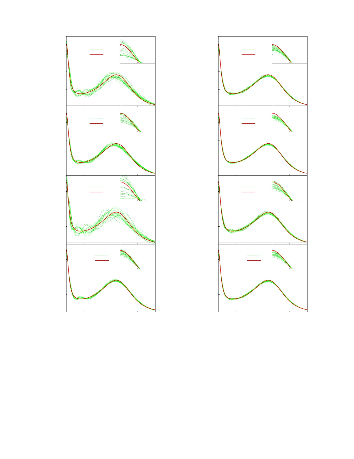
Analytical con tin uation of imaginary axis data using maxim um en tropy O. Gunnarsson (1) , M. W. Hav erkort (1) and G. Sa ngiov anni (2) 1 Max-Planck-Institut f¨ ur F est k¨ orp erforschung, D-70506 St uttgart, Germany 2 Institut f¨ ur F estk¨ orp erphysik, T e chnische Univers it¨ at Wien, Vienna, A ustria W e study the maximum en tropy (M axEnt) approac h for analytical continuatio n of sp ectral data from imaginary times to real frequencies. The total error is divided in a statistical error, due to the noise in the input d ata, and a systematic error, due to deviations of t he default function, used in the MaxEnt approach, from the exact spectrum. W e find that the MaxEnt approac h in its classical formulation can lead to a nonoptimal b alance b etw een the tw o typ es of errors, leading to an unnecessary large statistica l error. The statistical error can b e reduced by splitting up the data in sever al batc hes, p erforming a MaxEnt calculation for eac h batc h and ave raging. This can outw eigh an increase in the systematic error resulting from this approac h. The outpu t from the MaxEn t result can b e u sed as a default function for a new MaxEnt calculation. Such iterations often lead to worse results due to an in crease in the statistical error. By splitting up th e data in b atches, th e statistical error is reduced and and th e increase resulting from iterations can b e outw eighed by a decrease in the systematic error. Finally we consider a linearized versi on to obtain a better understanding of the method . I. INTRO DUCTION The ana lytical contin uation of sp ectra l functions from imaginary time τ to real energies ω is a difficult problem due to its ill-p os e d nature, i.e., the output can dep end very sensitively on the input. F or stro ngly cor r elated electrons, how ev er, this is an imp ortant problem. Most approaches for such systems in volv e uncontrolled appro x- imations. Using quantum Monte-Carlo (Q MC) methods or quantum cluster metho ds it is, how ever, p os sible to obtain accurate data fo r Green’s functions and resp ons e functions o n the imagina ry axis, ra ising the problem of analytical con tin uation to the rea l axis. Since these meth- o ds provide da ta with statistical noise, the ill-p osed na- ture of the problem makes analytical contin uation very difficult. This problem c an b e treated within the Bayesian theory . 1,2 The problem is r egularized by in tro ducing an ent ropy in terms of the deviation of the output real axis sp ectrum from s ome default function. The imp or- tance of the entropy is cont rolle d b y a parameter α , which is determined using s tatistical a r guments. 1,2 This metho d is referr ed to as the Maximum E ntropy (Max - Ent) metho d. It has b een ra ther succe s sful in p erfor ming analytical co ntin ua tions. Alter na tive methods have b een prop osed, s uch as Pad´ e approximations, 3,4 singular v alue decomp osition, 5 sto chastic reg ularizatio n 6 and sampling schemes. 7,8 In this pap er we focus on the MaxEnt method. This metho d is usually discusse d in terms of the Ba yesian the- ory . Her e we start from the equa tions generated b y the MaxEnt forma lism and use an algebraic appro ach to an- alyze the theory . W e discuss the ac curacy that can b e obtained within this framew ork. The error in the output sp ectral function ca n b e split up in a statistical error, due to the noise in the input data, and a systema tic er- ror, due to the devia tion o f the default function fro m the true sp ectrum. T he choice of α determines the rela tive size of these error s. In the cla s sical MaxE nt metho d the most probable α is chosen. 1 W e find that this choice can make the s tatistical e rror unnecessa ry lar ge. The input data is typically given as a num b er N sample of samples, ¯ G ν ( τ ), where each sample gives a (noisy ) version o f the imag ina ry time function G ( τ ). W e find that the a ccuracy can sometimes b e impr ov ed by split- ting up the samples in N calc sub sets (batches), with N sample / N calc samples in each batch. W e then p erfor m N calc MaxEnt calculatio ns, each with N sample / N calc sam- ples, and then av erage the results, instead of p erfor ming one MaxEnt calcula tion N sample samples. This approa ch reduces the statistica l error at the cost of an increase in the s ystematic error. W e also discuss the po ssibility of an iterative MaxEnt metho d, where the output is used to define a new de- fault function. This us ua lly works p o o rly , and we show that this is due to an increa s e in the statistical erro r , ov erwhelming the improvemen t in the systematic er ror. How ev er, if the data are split in ba tches, as discussed ab ov e, the impor tance of the statistical error ca n b e re- duced to the p o int where the appro ach impro ves the tota l accuracy . T o further analyze the r esults, we in tro duce an a lterna- tive method with a new, slightly different definition o f the ent ropy . This le a ds to a set of linear equations, where the propaga tion of the er rors ca n b e analy zed mor e ea sily and features of the MaxEnt method better understo o d. This metho d, how ever, do es no t guarantee a p ositive sp ectra l function, a nd it is less useful for pr actical calculations. In this pap er we focus o n a resp onse function, the op- tical conductivity σ ( ω ). W e int ro duce a typical σ ( ω ), which in the following will b e refered to as the “ exact” σ ( ω ). The form of σ ( ω ) w as chosen using results for the t wo-dimensional Hubbard mo del as a guide. This mo del of σ ( ω ) can easily and a c curately b e trans fo rmed to imag- inary axis data. W e add statistical noise to the data a nd then transfor m the data back to the re a l axis, using the v ar io us mo difica tions of the MaxEnt metho d. If a given metho d w orked p erfectly the σ ( ω ) that we star ted with 2 .0 .1 .2 .3 .4 0 1 2 3 4 5 6 σ ( ω ) ω Opt. cond. Model 1 Model 2 .25 .30 .35 .0 .1 FIG. 1: (color on-line) “Exact” sp ectral function and tw o different default mo dels as a function of frequency . The inset sho ws the mo dels on a small energy scale. should b e recovered exactly . The devia tions from the “exact” σ ( ω ) ar e then a measur e o f the accur acy o f the different approa ches. As an example, Fig. 1 s hows an “ex act” o ptical con- ductivit y and tw o de fa ult mo dels used in the MaxE nt ap- proach. The optica l co nductivit y has a Drude like p eak at ω = 0 and a “Hubbard” pea k at ω ∼ 3 corr esp onding to tr ansitions b etw een the Hubbard bands. The default mo dels ar e chosen so that they satisfy the exact sum rule. The tw o mo dels are ch osen according to tw o different strategies. It is sometimes arg ued that the default mo del should contain little informatio n, apart from certain ex- act results, s uch as sum rules. This wa y the results are not prejudiced by pos s ible incorrect assumptions. Mo del 1 has bee n chosen this wa y . Alternatively , a s a default mo del one can use the output from a calculation at a higher temper ature T . Mo de l 2 has therefore been cho- sen to b e quite similar to the “exac t” result, but with all features s o mewhat broa der. Mo del 2 will na tur ally deliver muc h more accurate o utput s pec tra. The pap er is organize d as follows. In Sec. I I we in- tro duce the formalism. Sec. I I I describ es how a Ma xEnt calculation is perfor med as an average of several MaxEnt calculations a nd Sec. IV discusses an iterative Ma xEnt metho d. In Sec. V w e present a simplified entrop y defi- nition, leading to linear equations. II. FORMALISM W e introduce the basic forma lism, ess e nt ially follow- ing Jarrell a nd Gub ernatis, 1 and then provide err or es- timates. The function G i = G ( τ i ) for imaginary time τ i is related to a sp ectra l function A i = A ( ω i ) on the real frequency axis ω , G i = N ω X j =1 K ij A j i = 1 , ...N τ , (1) via a kernel K ij = K ( τ i , ω j ), given for some discrete v alues ω j of ω . F or the case of the optical conductivity , considered her e, the kernel is given by K ij = 1 π ω j 1 − exp( − β ω j ) ( e − ω j τ i + e − ( β − τ i ) ω j ) f j , (2) where f j is a weigh t factor chosen so that Eq. (1) corr e- sp onds to a n integral ov er ω . F or the electron Gree n’s function the co rresp onding kernel is K ij = e − τ i ω j 1 + e − β ω j f j . (3) W e introduce a likelihoo d function L = 1 2 N τ X i =1 ( ¯ G i − G i σ i ) 2 , (4) where ¯ G i are data obtained from, e.g., a Monte-Carlo calculation, w ith the s tatistical ac curacy σ i , a nd G i has bee n calculated from E q (1). W e a lso intro duce the en- tropy S = N ω X i =1 f i ( A i − m i − A i ln A i m i ) , (5) where m i is a default mo del. The quantit y L − αS is then minimized with re s pe ct A j . This leads to the equa tions − N τ X i =1 ¯ G i − G i σ 2 i K ij + αf j ln A j m j = 0 (6) These equations are so lved to obtain the sp ectral function A i . The quantit y α can b e deter mined using statistical metho ds, giving the most probable α . This is referred to as the classica l MaxEnt metho d. 1 Alternatively , o ne ca n av erage the spectrum calculated for different v alues of α , using the pro bability o f tha t α a s a weigh ting function. 1 This metho d, Bryan’s metho d, gives similar results for the c ases cons idered her e. T o estimate the error in this approa ch, we ex press the calculated sp ectral function A in terms of the exact r e sult A exact as A i = A exact i + ∆ A i , (7) where ∆ A i is the erro r in A i . W e assume that the erro r is sufficiently small that the loga rithm in Eq. (6) can b e expanded to lowest o rder. Then − N τ X i =1 ∆ ¯ G i − ∆ G i σ 2 i K ij + αf j (ln A exact j m j + ∆ A i A exact i ) = 0 , (8) where ∆ G i = P j K ij ∆ A j and ∆ ¯ G i = ¯ G i − P j K ij A exact j is the error in ¯ G i due to the s tatistical noise. T o solve these equa tions, we define a j = N τ X i =1 ∆ ¯ G i K ij σ 2 i + αf j ln m j A exact j (9) 3 b j k = N τ X i =1 K ij K ik σ 2 i + αf j A exact j δ j k . (10) Using matr ix nota tions, ∆ A = b − 1 a = b − 1 K T σ − 2 ∆ ¯ G + b − 1 αf ln( m A exact ) . (11) The error w is defined a s w = h N ω X i =1 (∆ A i ) 2 f i i ≡ w stat + w syst , (12) where h ... i denotes the average ov er many different real- izations of the noise ∆ ¯ G i in the input data. Here w stat is the er ror due to this noise and w syst is the er ror due to the deviation ∆ m i = m i − A exact i (13) of the default function fro m the exact r esult. Since the noise is r a ndom, there is no co nt ribution from the cro ss term in the squar e o f the tw o terms in Eq. (11). The statistical error can then b e written as w stat = h N τ X j,k =1 ∆ G j σ 2 j ( K b − 1 f b − 1 K T ) j k ∆ G k σ 2 k i (14) = N τ X j =1 ( K b − 1 f b − 1 K T ) j j σ 2 j = T r σ − 2 K b − 1 f b − 1 K T . The seco nd equality w as o btained by noticing that the terms j 6 = k do not co nt ribute on the average and that the av erag e of ∆ G 2 i is σ 2 i . Later we consider the average ov er N calc MaxEnt calculatio ns, each using data with the statistical accura cy σ . The statistica l error w stat is then reduced by a factor of N calc , sinc e w stat refers to the square o f the er ror in the output s pe c tr um. F or the systematic erro r we obtain w syst = ln( m A exact ) f αb − 1 f b − 1 αf ln( m A exact ) . (15) The re s ults in Eqs. (1 4, 1 5) a pply to the cas e when Max- Ent calc ulation is not itera ted. F or an itera tive ca lcula- tion we use Eq. (22) b elow. Fig. 2 shows w stat and w syst as a function of α for different σ . The figure illustrates that w stat behaves ap- proximately as 1 / α . This illustrates the imp orta nc e of int ro ducing entrop y , i.e., using an α > 0. F or α = 0, the matrix b − 1 is ill- be hav ed a nd the statistical err or would be huge. Since w stat depe nds o nly weakly on σ , it is not po ssible to make w stat small for α = 0 b y simply reducing σ (within reaso nable limits). Introducing α > 0 r egular- izes b a nd leads to a ma na geable statistical err or. The systematic erro r increases with α and there is therefore an o ptimal v a lue of α where the total erro r is minim um. The dependence o f the systematic error on σ is sho wn in Fig. 3. It b ehaves ro ughly as √ σ . The optimal α there- fore increa ses as σ is reduced. It also increase s as the -12 -10 -8 -6 -4 0 2 4 6 8 10 log(w stat ) log( α ) σ =0.0001 σ = 0.001 σ = 0.01 σ = 0.1 -11 -10 -9 -8 -7 -6 -5 -4 -3 0 2 4 6 8 10 log(w syst ) log( α ) σ =0.0001 σ = 0.001 σ = 0.01 σ = 0.1 FIG. 2: (color on- line) Statistical ( w stat ) [Eq. (14)] and sys- tematic ( w syst ) [Eq. (15)] errors for default mo del 1 as a func- tion of α and for different v alues of σ . The parameters are β = 15 and N τ = 60. -12 -11 -10 -9 -8 -7 -6 -5 -4 -9 -8 -7 -6 -5 -4 -3 -2 log(w syst ) log( σ ) Model 1 α =40 Model 2 α =40 Model 1 α =200 Model 2 α =200 Model 1 α =1000 Model 2 α =1000 -12 -11 -10 -9 -8 -7 -6 -5 -4 -9 -8 -7 -6 -5 -4 -3 -2 log(w syst ) log( σ ) 0.001 σ 1/2 FIG. 3: (color on-line) Systematic error ( w syst ) [Eq. (15)] for default mo dels 1 and 2 as a funct ion of σ and for different v alues of the α . The straight line sho ws the curve 0 . 001 σ 1 / 2 , illustrating that w stat is approximately prop ortional to √ σ . The parameters are β = 15 and N τ = 60. 4 -11 -10 -9 -8 -7 -6 -9 -8 -7 -6 -5 -4 -3 -2 log(w) log( σ ) x w stat (N calc =1) w syst (N calc =1) w stat (N calc =5) w syst (N calc =5) -11 -10 -9 -8 -7 -6 -9 -8 -7 -6 -5 -4 -3 -2 log(w) log( σ ) x w(N calc =1) w(N calc =5) FIG. 4: (color on-line) S tatistical ( w stat ), systematic ( w syst ) and total ( w ) errors in a MaxEnt calculation for the sp ectrum in Fig. 1, default mo del 1, α = 40 and β = 15 and 100 samples, eac h with the accuracy σ . The full thick (red) line shows w when one ( N calc = 1) MaxEnt calculation is p erformed for the a verage of ov er all data and the the thic k broken (blue) line t he result when N calc = 5 MaxEnt calculations are a veraged, eac h calculation using the av erage of 100 / N calc samples. The cross corresponds to a historic MaxEnt calculation for σ = 0 . 01, whic h gives α ≈ 40, used in the fi gure. The thick broken (blue) curve illustrates that a sub stantia lly lo wer error can b e obtained by av eraging 5 MaxEnt calculations. default mo del is made more accura te, e.g., by replacing default model 1 by mo del 2. Since ω = 0 is often of particular in terest we use a logarithmic ω -mesh. F or the case 0 ≤ ω ≤ ω max we use ω i = exp[( i − 1) dx + ln γ ] − γ , (16) where dx = [ln( ω max + γ ) − ln γ ] / ( N ω − 1). A small v alue of γ leads to a smaller spacing of the p oints close to ω = 0. W e hav e t ypically used N ω = 121 p oints, γ = 0 . 5, ω max = 12, β = 15 and N τ = 60. F o r s implicit y , we assume that the statistica l er r or is given by σ i = G i σ , (17) in terms of so me ov erall acc uracy σ . T o p erform these calculations we hav e develop ed a MaxE nt co de, which was found to give almost identical r esults to a code made av ailable to us b y Jarr ell. 1 II I. MUL TIPLE MAXENT CALCULA TIONS A Q MC ca lculation is arrang ed s o tha t it gives a n um- ber o f samples, ¯ G ν ( τ i ), of G ( τ i ). F r om thes e data one can ca lc ula te the statistical accura cy σ i , chec k if the da ta are Gaussian and c heck for (undesirable) corre lations b e- t ween the noise for differ ent v alues of τ . 1 The data ¯ G ν ( τ i ) are then av eraged ov er ν to obtain ¯ G ( τ i ) that is the in- put for the MaxEnt calculation, p ossibly after removing correla tions betw een the noise at different τ -p o int s. 1 T ABLE I: Statistical ( w stat ), systematic ( w syst ) and total ( w ) error in MaxEn t calculations for the sp ectrum in Fig. 1 and default mo dels 1 or 2. 100 samples, each with the accuracy σ , w ere split up in N calc batches with 100/ N calc samples an d u sed in N calc calculations. The av erage of the output w as u sed as a d efault mo del, p erforming N iter iterations. The errors were obtain from Eqs. (14, 15) for N iter = 1 and from Eq. (22) for N iter > 1. The p arameters w ere β = 15 and N τ = 60. Default model α N calc N iter w stat w syst w 1 40 1 1 6.7 10 − 4 1.4 10 − 4 8.1 10 − 4 1 40 5 1 1.4 10 − 4 2.1 10 − 4 3.5 10 − 4 1 40 1 2 14 10 − 4 1.3 10 − 4 15 10 − 4 1 40 100 4 0.4 10 − 4 0.9 10 − 4 1.3 10 − 4 2 720 1 1 4.2 10 − 5 4.4 10 − 5 8.6 10 − 5 2 720 2 1 2.3 10 − 5 5.6 10 − 5 7.9 10 − 5 2 720 1 2 9.7 10 − 5 3.3 10 − 5 13 10 − 5 2 720 20 8 2.4 10 − 5 3.9 10 − 5 6.3 10 − 5 W e now consider the cas e where we have 100 sam- ples, eac h with the acc uracy σ . After av erag ing ov er all the samples , the accur acy of the resulting data is σ / √ 100 = σ / 10 . The v a lue of α in a classic a l Max- Ent calculation depends o n the sp ecific realization of the noise. W e therefore per form many calcula tions, each with a different realiza tion of the no ise, a nd av erage over α . F or σ = 0 . 01 , β = 15 and N τ = 60, classical MaxEnt calculations using the sp ectrum in Fig. 1 a nd the default mo del 1 then gave o n the av erag e α ≈ 40. Fig. 4 shows the sta tistical and systematic er rors for a fixed α = 40 as a function of σ ( N calc = 1). T he cr o ss gives the total error of a clas sical MaxEnt calculation corres p o nding to 10 0 s amples with σ = 0 . 01. The figure illustrates that the statistical erro r is m uch la rger than the systema tic error for the Ma xEnt calculation. This is als o illustrated in Fig. 5a. This shows the res ult of 20 MaxEnt calculations with different realiza tions o f the noise, ea ch with 100 sa mples with the accura c y σ . The thic k (red) line shows the exact sp ectrum. The calcula ted sp ectra (thin gr e en lines) scatter strongly ar ound the ex- act r esult, illustrating a la rge statistical erro r. On the av erage, these sp ectra a lso deviate s omewhat from the exact result, the v alue of σ (0) being slight ly to o small and the Hubbard p eak being somewhat shifted tow ards low er energies , illustrating a small sy s tematic er ror. W e next gr oup the 1 00 samples in N calc = 5 batches, each with 20 samples, and per form N calc MaxEnt calcu- lations. The ac c ur acy of the data in these Ma xEnt cal- culations is then only √ N calc σ / 10. This increa ses b oth the systematic and statistical err ors so mewhat. Av er- aging these calculatio n, howev er, reduces the statistical error b y a factor N calc . In Fig. 4 this leads to a large net reduction in the statistical er r or, which more than com- pens ates for the increase of the systematic erro r. This is illustrated in Fig. 5b, which s hows 20 such results, each one obtained by averaging N calc = 5 MaxEnt cal- culations with 100 / N calc samples, but with different r e - 5 0 0.1 0.2 0.3 σ ( ω ) a) N iter =1 N calc =1 Exact .25 .30 .35 .0 .1 0 0.1 0.2 0.3 σ ( ω ) b) N iter =1 N calc =5 Exact .25 .30 .35 .0 .1 0 0.1 0.2 0.3 σ ( ω ) c) N iter =2 N calc =1 Exact .25 .30 .35 .0 .1 0 0.1 0.2 0.3 0 1 2 3 4 5 σ ( ω ) ω d) N iter =5 N calc =100 Exact .25 .30 .35 .0 .1 FIG. 5: (color on- line) Optical cond uctivity calculated for the default model 1 using different metho ds. 100 samples, eac h with the accuracy σ = 0 . 01 were given. a) Eac h curve show s results of a classical MaxEnt calculation using an av erage of all 100 samples. The figure shows 20 such curves, eac h corre- sp on d ing t o a different realization of th e n oise. b) Each curve sho ws the a verage of N calc = 5 MaxEnt calculations using 100/ N calc samples. c) Eac h curve sho ws the results of iterat- ing th e calculations in a) once, using the output in a) as a de- fault function in the next MaxEnt calculation. d) Each curve sho ws th e results of iterating MaxEnt calculations N iter = 5 times. N calc = 100 was used, and the default function was obtained from the a verage of th ese N calc calculations. The parameters were β = 15, N τ = 60 and α = 40. 0 0.1 0.2 0.3 σ ( ω ) a) N iter =1 N calc =1 Exact .25 .30 .35 .0 .1 0 0.1 0.2 0.3 σ ( ω ) b) N iter =1 N calc =2 Exact .25 .30 .35 .0 .1 0 0.1 0.2 0.3 σ ( ω ) c) N iter =2 N calc =1 Exact .25 .30 .35 .0 .1 0 0.1 0.2 0.3 0 1 2 3 4 5 σ ( ω ) ω d) N iter =5 N calc =100 Exact .25 .30 .35 .0 .1 FIG. 6: (color on-line) The same as Fig. 5, b ut starting from the default model 2 and u sing α = 720. alizations of the nois e. The spr ead b etw een the cur ves is substantially smaller ( w stat = 0 . 0 0014 vs. 0.0 0067) than in Fig. 5a, while the systema tic error is somewhat larger ( w syst = 0 . 00 021 vs. 0.00 014). This leads to a substantial improv ement in the total err or ( w = 0 . 0003 5 vs. 0.00 081). These results a re a lso shown in T able I. The reas on for this improv ement is that that w stat ≫ w syst in the MaxEnt ca lculation with N calc = 1 and tha t w stat and w syst hav e different dep endencies on N calc . F o r 6 α = 0, Eq. (14 ) gives that w stat ∼ σ 2 . Splitting up the calculation in N calc calculations makes the effective σ a factor √ N calc larger , while averaging reduces the e r ror by a factor N calc . The net result w ould be an unchanged statistical erro r. It is therefore crucia l that the metho d has be e n regular ized by in tro ducing an entrop y . Fig. 4 shows that for realistic v alues o f α , w stat actually has a quite weak dep endence on σ , rather than b ehaving as σ 2 . Splitting up the samples in several batches, and thereby reducing the accur acy of each batch, leads to a s ma ll increase in w stat for each individual calc ulation. The av- eraging over N calc calculations, how ever, reduces w stat by a factor N calc . A t the same time w syst is incr eased, but only by approximately a factor N 1 / 4 calc , since this quant ity behaves approximately as √ σ and σ incr eases by a factor √ N calc . Fig. 6 and T able I show the corre s p o nding r esults us- ing default mo del 2. In this case the classica l Ma xEnt calculation choose s a v alue of α that ma kes w stat and w syst comparable. The gain from splitting up the sa m- ples and p erforming several MaxEnt calculations is then m uch smaller. W e ar e now in the p os ition to dis c uss the limits of accuracy that can b e obtained in this approach. W e con- sider as b efore 1 00 samples with the a ccuracy σ = 0 . 0 1 and allow for a ny co m bination of α , N calc ≤ 10 0 and N iter ≤ 40. Starting from default mo del 1, we o bta in the results shown in Fig. 7a. The cur ve “One calc.” shows the result o f a tr aditional Ma xEnt calculation, using all the samples in one calculation ( N calc = 1 and N iter = 1). If a classical MaxEnt ca lculation is p e rformed, α ≈ 2 0 is obtained. This result is s hown b y a cro ss. W e can s ee that this v alue of α is not o ptimal, and a lar ger α would hav e given a smaller err or. W e next allow for N calc > 1 calculations, each using 100 / N calc samples. W e find the v alue o f N calc which gives the b es t ag r eement with the “exact” σ ( ω ). This (“Several o pt.”) leads to a muc h higher accurac y fo r small v a lues of α . The curve is al- most fla t as a function o f α ov er a substantial range. F or large v alues o f α , N calc = 1 gives the b est a c c uracy , and the c urve falls o n top of the cur ve “One calc.”. T o provide a criter ion for how to split up the da ta in batches, we consider the statistical er r or [(Eq. 14)] again. As b efore we cons ide r the case of N sample samples, each with the a ccuracy σ , divided in N calc batches with N sample / N calc samples in ea ch. W e define the pro duct M ( σ ) = b − 1 K T σ − 2 , (18) where b als o depends on σ . The statistical error o f the k th calculation is then written as ∆ A ( k ) i = N τ X j =1 M ij ( σ N calc ) N calc N N/ N calc X ν =1 ∆ ¯ G ν +( k − 1) N/ N calc j , (19) where ∆ ¯ G ν is the error in the ν th sa mple, and the sta- tistical accuracy σ N calc = σ / p N / N calc ent ers due to the av eraging over N / N calc samples. W e then av erag e ov er -9 -8.5 -8 -7.5 -7 -6.5 -6 -5.5 3 4 5 6 7 8 9 log(w) log( α ) x Default mod. 1 One calc. Several opt. Several est. Iterated -10.5 -10 -9.5 -9 -8.5 -8 -7.5 -7 -6.5 -6 -5.5 3 4 5 6 7 8 9 log(w) log( α ) x Default mod. 2 One calc. Several opt. Several est. Iterated FIG. 7: (color on-line)Accuracy w of MaxEnt calculations for 100 samples, each with accuracy σ . ”One calc.” uses the av er- age of all samples in one MaxEnt calculation. ”Several opt.” and “Several est.” split up the samples in several batches and a verages th e resulting MaxEnt calculations. ”Several opt.” does this in t he op t imal wa y and “Severa l est.” uses a pre- scription for fin ding the splitting when the exact result is not known. ”It erated” in addition uses th e ou t put sp ectral func- tion as d efault mo del in an iterative approach. The cross sho ws the result of a classical MaxEnt calculation. a) shows results for default mo del 1 add b) for default mo del 2. The parameters are β = 15 and N τ = 60. the N calc calculations and o btain the err or ∆ A i = N τ X j =1 M ij ( σ N calc ) 1 N N X ν =1 ∆ ¯ G ν j . (20) The av erage difference b etw een t wo c a lculations with N calc and M calc batches can then b e written as w M N ≡ X i [ A i ( N calc ) − A i ( M calc )] 2 w i = (21) X ij w i [ M ij ( σ N calc ) σ N calc √ N calc − M ij ( σ M calc ) σ M calc √ M calc ] 2 . This result repr esents an av erag e over many differen t re- alizations of the err or ∆ ¯ G ( k ) . In addition to the sta- 7 tistical contribution to the difference there is a s ystem- atic contribution due to the error in the default function. W e then compar e calc ula tions with N calc = N sample and M calc = N sample / 2 batches. In the seco nd c alculation the statistical error is large r and the systema tic erro r is smaller. If the to ta l difference betw een the t wo calcula - tions is larger than twice the exp ec ted statistical differ- ence, this sug gests that the ga in in the s y stematic err or outw eighs the loss in the statistica l erro r a nd the seco nd calculation is accepted. W e then compar e this calcula - tion with a calculation with N sample / 4 batches and if the latter is fa vorable the pro cedure is contin ued, consider- ing N sample / 10, N sample / 20 a nd N sample / 50 batches. The resulting a ccuracy is shown by the curves “ Several es t.” in Fig. 7. This curve is ab ove the curve “Several opt.”, but the difference is not very large for most v alues of α . IV. ITERA TING MAXENT Once a Ma xEnt calculation has be e n p erformed, one can tr y to improv e the defa ult function b y using the out- put sp ectral function as a new default function. Such an iterative approa ch, howev er, is usually no t recommended. Fig. 5c shows the results o f s uch calcula tio ns using de- fault model 1. Indeed, the spread betw een b etw een dif- ferent calc ulations is large r than in the nonitera ted case in Fig. 5a , implying an increased statistical error. Eqs. (14, 15) used to calculate the statistical and sy s - tematic errors for a nonitera ted default mo del are not appropria te in the case of iterations. The reason is that the default model in this c ase co nt ains statistical err ors due to the iteration pro cedure. Instead we per form ma ny calculations N of the type shown in Fig. 5c, giving sp ec- tral functions A ν i , ν = 1 , .., N . W e then calculate A av i = 1 N N X ν =1 A ν i w stat = 1 N − 1 N X ν =1 N ω X i =1 ( A ν i − A av i ) 2 f i (22) w syst = N ω X i =1 ( A av i − A exact i ) 2 f i Due to nonlinearity , s ome o f the statistical er ror actually shows up as a sy stematic er ror in Eq. (22), but this is neglected in the following. The results in T able I, shows that the statistica l er- ror is mor e than do ubled after one iteration, while the systematic error is not cor r esp ondingly reduced. W e next consider the case when the samples are split up in N calc batches and default mo del 1 is used. Using N calc = 100 a nd N iter = 4 the total er ror is r educed, as is illustrated in Fig. 5d and T a ble I. By using N calc = 100 , we drastically reduce the statis tica l er r or. The following iterations incr ease the sta tistical err o r by a substa nt ial factor, but it nevertheless rema ins sma ll. A t the same time the iter ations r educe the sys tematic err or, so tha t bo th are improved compared with the noniter ated case. Fig. 6d shows similar results using defa ult mo del 2. Since this mo del is very close to the ex act result, iterations now lead to a small improv emen t, but even with such an accurate default function there is an improv emen t. In Fig. 7, the curve “Iterated” shows r esults when iteratio n is allowed ( N iter ≤ 40). This lea ds to a substantial im- prov ement in the accur acy . Fig. 7 b shows similar r esults for defa ult mo del 2. V. QUADRA TIC ENTROP Y In Eq. (6) in Sec. I I we introduced the entrop y , con- taining a loga r ithm. As a result, the basic equations of MaxEnt are nonlinear, which makes the a nalysis compli- cated. F or this re a son, we intro duce a new definition o f the entropy , which is used in this sectio n for analyzing the b ehavior of MaxEnt. The expressio n in Eq. (5) is expanded to lowest (seco nd) o rder in the deviatio n b e- t ween the solution and the default function. W e then define this as the en tropy , and use it in this section. This is then not an appr oximation but simply a ne w metho d. This metho d has s ome pro blems. F or instance, it is not guaranteed that the sp ectrum is p os itive. Therefore we do no t reco mmend the use o f this metho d for ca lculating sp ectra, but simply use it to analyze Max Ent. W e define the entrop y S = − 1 2 N ω X i =1 f i ( A ( n ) i − m ( n ) i ) 2 m ( n ) i , (23) where we hav e allow ed for the p ossibility of the MaxEnt calculation being itera ted, i.e., m ( n ) depe nds on the iter - ation n . The o riginal default function is m (0) . This lea ds to the equations a = K T σ − 2 ¯ G + αf (24) b ( n ) = K T σ − 2 K + αf m ( n ) where matrix notatio ns hav e b een used and αf and αf /m ( n ) are diagonal matrices . Then A ( n +1) = [( b ( n ) ] − 1 a . The err or in A ( n +1) is ∆ A ( n +1) = [ b ( n ) ] − 1 [ K T σ − 2 ∆ ¯ G + αf ∆ m ( n ) m ( n ) ] , (25) where ∆ m ( n ) = m ( n ) − A exact . W e define δ G ( n ) = s m ( n ) αf K T σ − 2 ∆ ¯ G δ A ( n ) = r αf m ( n ) ∆ A ( n ) (26) c ( n ) = r αf m ( n ) [ b ( n ) ] − 1 r αf m ( n ) 8 and a similar definition for δ m ( n ) as for δ A ( n ) . P i [ δ A ( n ) i ] 2 contains the same integration factor f i as has bee n use d earlier , but due to the factor 1 /m ( n ) it gives more w eight to er rors where m ( n ) is small. W e have δ A ( n +1) = c ( n ) [ δ G ( n ) + δ m ( n ) ] . (27) W e find the eigenv alues ε ( n ) ν and eig e nv e ctors | ν ( n ) i of the symmetric matrix c ( n ) . Introducing the expansion in these eigenv ectors, δ A ( n ) ν = h ν ( n ) | δ A ( n ) i we obtain δ A ( n +1) ν = ǫ ( n ) ν [ δ G ( n ) ν + δ m ( n ) ν ] . (28) The matrix c can b e rewritten as c ( n ) = [ s m ( n ) αf K T σ − 2 K s m ( n ) αf + 1] − 1 (29) F or the cas es we hav e consider ed, the first matrix inside the bra cket has a broad rang e of po sitive eig e nv a lues, ex- tending fro m eigenv alues muc h smaller than one to muc h larger than o ne . As a result, the matrix c ( n ) is found to hav e so me very small eigenv alues and many eigenv alues very clo se to one. This is illustra ted in T a ble I I, which shows the lowest eigenv alues for the default model 1 and α = 40 . Fig. 8 shows the eigenfunctions | ν (0) i cor resp onding to the low e st eigenv alues in T able I. The lowest func- tion is no de le s s, and the hig her functions have a n in- creasing n umber o f no des. F unctions with the eigenv alue very close to one o scillate so rapidly that the co rresp ond- ing comp o nents of δ m ( n ) ν and δ G ( n ) ν tend to hav e small weigh ts, as shown in T able II. As a compa rison, T able I I also shows the expansion co efficients o f the default mo del 2 in the eigenfunctions obtained for the default mo del 1 and α = 40. It is crucial fo r the success of a MaxEnt c a lculation that the co efficients δ m ( n ) ν and δ G ( n ) ν are t ypically small for ε ( n ) ν close to one. F r om Eq. (28) it follows that err ors δ m ( n ) ν and δ G ( n ) ν corres p o nding to eigenv alues ε ν m uch smaller than one give a str ongly r e duce d contribution to the er ror δ A ( n +1) ν , while er rors corr e s p o nding to the eigenv alue one are not r educed at all. F or these comp o- nent s the devia tion o f the default mo del fro m the true result a re ta ken ov er completely . A t the sa me time this sets the limits for MaxE nt calcu- lations. A MaxE nt ca lculation fails if A ( ω ) has s tructures on such a small energy sca le that there are impo rtant ex - pansion c o efficients δ A ( n +1) ν corres p o nding to eigenv alues close to one, since the MaxE nt calculation gives no ad- ditional information ab out these comp onents. This als o shows the dange r of putting in to o muc h structure on a small e ne r gy scale in the default function. This would make co mp o nents δ m ( n ) ν corres p o nding to ε ν ≈ 1 im- po rtant and the MaxEnt ca lculation would not r emov e them from A ( n +1) ν , even if there is no supp or t for such comp onents in the data . The results in Figs. 5 a nd 6 show a b eating patter n, where the different calculatio ns a gree appr oximately fo r certain v alues of ω . This must b e related to the noise in the input data , sinc e this is what differs b etw een the calculations. The reaso n can b e see n from T able I I and Fig. 8. The contribution of the noise to the output is given by ε ν δ G ( n ) ν . This contribution comes mainly from the eighth and ninth eigenv alues. The corr esp onding eigenfunctions in Fig. 8 have their zero s approximately where the deviations b etw e e n the calcula tio ns in Fig . 5 are small, althoug h the ag reement is not p er fect. The reason is probably the nonlinearity due to the loga rithm in Eq. (11). F or instance, if the logar ithm is expanded to second order , the resulting pro duct o f tw o functions generates functions with mo re no des than either of the t wo functions. As a r esult w e find that δ A ( n +1) ν has ap- preciable err ors also for comp o ne nts with a few mo re no des than the eig hth and ninth eigenfunctions. This then shifts the b eating pattern slightly towards low er en- ergies. W e introduce the pro jectio n op era tor P ( n ) = X ν | ν ( n ) ih ν ( n ) | Θ( ε 0 − ε ( n ) ν ) , (30) where the Θ-function selects states with e igenv alues smaller than ε 0 < 1 . Eq. (28) c an now b e itera ted. If we assume that ǫ ( n ) ν is indep endent of n , whic h is a go o d approximation, we obtain δ A ( n +1) ν = ( P n +1 i =1 ε i ν δ G (0) ν + ε n +1 ν δ m (0) ν for ε ν ≤ ε 0 ε ν [ δ G (0) ν + δ m (0) ν ] for ε ν > ε 0 (31) This illustrates how iter a tion reduces the sy s tematic er- ror for comp onents with ε ν ≤ ε 0 , but incr eases the statis- tical error . Whether iteration pays off then dep ends o n the relative size of the statistical and s ystematic error s and the choice o f ε 0 . In this linear ized version, how ever, it do es not pay off to include a ll states in the pr o jection op erator (leading to P ( n ) ≡ 1). F or the nonlinear case, the b ehavior is a bit different. F r o m the expr ession for the error in E q. (11), it follows that ln ( m/ A exact ) en ters. Expa nding the logarithm leads to terms with pro ducts o f eig enfunctions of the t yp e in Fig. 8. Such pro ducts couple to higher eigenfunctions with more no des. The r esult is that the erro r of a certain ν -comp onent o f ln( m/ A exact ) dep e nds not only on the error of that ν - c omp onent of m but also o n the erro r s of o ther comp onents, in particular lower ones . Whether the err ors from the different contributions add constr uc- tively or destructively depends on the sp ecifics of the mo del. F or the cases w e co ns idered the contributions to the higher compo nents often add destr uctively . Then it can b e more fav orable to itera te all comp onents rather than just the o nes that would b e fav orable according to Eq. (31). F or the ca ses we ha ve studied, this has usually bee n the case a nd this is the appro ach we used in Sec. IV. 9 T ABLE I I: Low est eigenv alues ε ν of the matrix c (0) [Eq. (26)] and the correspondin g amp litu d es δ m (0) ν (1) and δ G (0) ν for default mod el 1. The v alues of δ m (0) ν (2) for default mod el 2 (expanded in th e functions corresponding to default model 1) and the expansion co efficien ts of σ ( ω ) are also sho wn. The larger eigen v alues are all close to unity , th e amplitudes of the corresp onding δ G (0) ν are all smaller than 2 10 − 4 . The corresp onding v alues of δ m (0) ν are also fairly small, smaller than 0.1 for default model 1 and smaller than 0.02 for default model 2. W e used β = 15, N ω = 121, ω max = 12, α = 40 and σ = 0 . 001. ε ν .3 10 − 6 .2 10 − 5 .6 10 − 5 .30 10 − 4 .2 10 − 3 .002 .016 .166 0.747 0.982 0.999 1.000 1.000 δ m (0) ν (1) -.92 -.81 -.28 -1.7 1.1 -.01 -1.1 -.17 .31 -.08 -.33 -.15 .007 δ m (0) ν (2) .80 -.32 .06 -.08 .08 .03 - .19 -.11 .07 .03 -.10 -.0 8 -.007 σ ν 3.1 -2.4 2.9 1.5 - 1.3 .09 1.0 .18 -.31 .08 .33 .16 -.007 q h ( δ G (0) ν ) 2 i 1. 6 10 3 675 371 1 76 65 23 7.90 2.1 .55 0.14 .03 .006 .001 ε ν q h ( δ G (0) ν ) 2 i .6 10 − 3 .002 .002 .005 .014 .038 .128 .349 .411 .134 .030 .006 .001 -0.2 -0.1 0 0.1 0.2 0.3 0 1 2 3 4 5 6 7 z( ω ) ω a) ε =.3 10 -6 ε =.2 10 -5 ε =.6 10 -5 -0.2 -0.1 0 0.1 0.2 0.3 0 1 2 3 4 5 6 7 z( ω ) ω a) ε =0.00003 ε =0.00020 -0.2 -0.1 0 0.1 0.2 0.3 0 1 2 3 4 5 6 7 z( ω ) ω a) -0.15 -0.1 -0.05 0 0.05 0.1 0.15 0.2 0 1 2 3 4 5 6 7 z( ω ) ω b) ε =0.002 ε =0.016 ε =0.166 -0.15 -0.1 -0.05 0 0.05 0.1 0.15 0.2 0 1 2 3 4 5 6 7 z( ω ) ω b) ε =0.747 ε =0.982 -0.15 -0.1 -0.05 0 0.05 0.1 0.15 0.2 0 1 2 3 4 5 6 7 z( ω ) ω b) FIG. 8: (color on-line) Eigenfunctions to the matrix c ( n ) in Eq. (26) corresponding to the 10 lo w est eigen v alues. The fig- ure illustrates how eigenfunctions correspondin g to an eigen- v alue close to one oscillate very rapidly . VI. SUMMAR Y W e have ana lyzed the MaxEnt a pproach for analyti- cal contin ua tion, defining a s tatistical error , due to noise in the imaginary axis input data, and a systematic error, due to er rors in the default function en tering the entrop y . The classica l metho d for choo sing the weigh t α of the en- tropy can lead to a nonoptimal choice, reducing the sys- tematic err or at the cost o f making the statistical erro r unnecessarily large. W e find that the statistical erro r can be reduced by splitting up the data in batches. A Max - Ent calculation is pe r formed for each batch and the res ult is averaged. This a ppr oach incr eases the s ystematic er ror but the total erro r can be reduced. W e hav e also studied an itera tive appr oach, where the output sp ectrum is used as default function in a new Max E nt calculation. W e find that a s traightforw ard applica tion of this approach often gives worse r esults due to a rapid increas e of the sta- tistical er ror. By splitting up the da ta in batches, the statistical err or can b e reduced sufficiently tha t this is less serio us. The reduction of the sy stematic err o r can then o utw eig h the increase of the statistica l err or. T o analyze Ma xEnt metho d, we hav e studied a lin- earized version of the problem. In this for malism it is easier to see how the statistical e r ror propaga tes, in par- ticular in the cas e o f iteratio ns . O ne ca n also s ee how certain deviations of the de fa ult function fro m the exact result have little influence on the output, while others fully show up in the o utput. This illustrates the danger of having a default function with to o m uch structure. While this pa p er shows the p otential for improving the MaxEnt metho d, it is ha rder to provide pr escriptions for how to use this. In Sec. I I I w e provided a prescription for how to split the data in ba tches, whic h we have fo und to often work fairly well for a g ive v alue of α . This metho d makes the res ulting error less sens itive to the optimiza- tion of alpha. Alternatively , one can simply split the data in, say 1 0, batches. F o r each batch the classica l metho d of determining α is used and the resulting MaxEnt results are av erag ed. This appr oach typically improv es the ac- curacy of the output s pe c trum. In pa rticular, it r educes the ris k o f finding spurious structures due to overfitting of no isy data , while some re a l structure s can be los t in this approach. 10 VII. ACKNO WLEDGMENTS W e w ould like to thank M. Jarrell for making his Max- Ent pr ogra m av aila ble. O ne of us (GS) wan ts to thank for s uppo rt through the FWF “Lise-Meitner” grant n. M1136. 1 M. Jarrell and J.E. Gub ernatis, Phys. Rep . 269 , 133 (1996). 2 R. N. Silver, D. S. Sivia, and J. E. Gub ernatis, Phys. Rev. B 41 , 2380 (1990); J. E. Gub ernatis, M. Jarrell, R. N. Silv er, and D. S. Sivia, Phys. Rev. 44 , 6011 91991); W . von der Linden, Appl. Ph ys. A 60 , 155 (1995). 3 H. J. Vidb erg and J. W. S erene, J. Lo w T emp . Phys. 29 , 179 (1977). 4 G. A. Baker, Jr., Essentials of Pad ´ e appr oximants A ca- demic, New Y ok, 1975, p 100ff. 5 C.E. Creffield, E.G. Klepfish, E.R. Pike, and S. Sark ar, Phys. Rev. Lett. 75 , 517 (1995). 6 I.S. Kriv enko and A.N. R ubtsov, arXiv:cond-mat/0612233 7 A. S. Mishchenk o, N . V. Prokof ’ev, A. Sak amoto, and B. V. Svistunov, Phys. Rev . B 62 , 6317 (2000). 8 K. V afayi and O. Gunnarsson, Phys. R ev. B 76 , 035115 (2007).