Stream sampling for variance-optimal estimation of subset sums
From a high volume stream of weighted items, we want to maintain a generic sample of a certain limited size $k$ that we can later use to estimate the total weight of arbitrary subsets. This is the classic context of on-line reservoir sampling, thinki…
Authors: Edith Cohen, Nick Duffield, Haim Kaplan
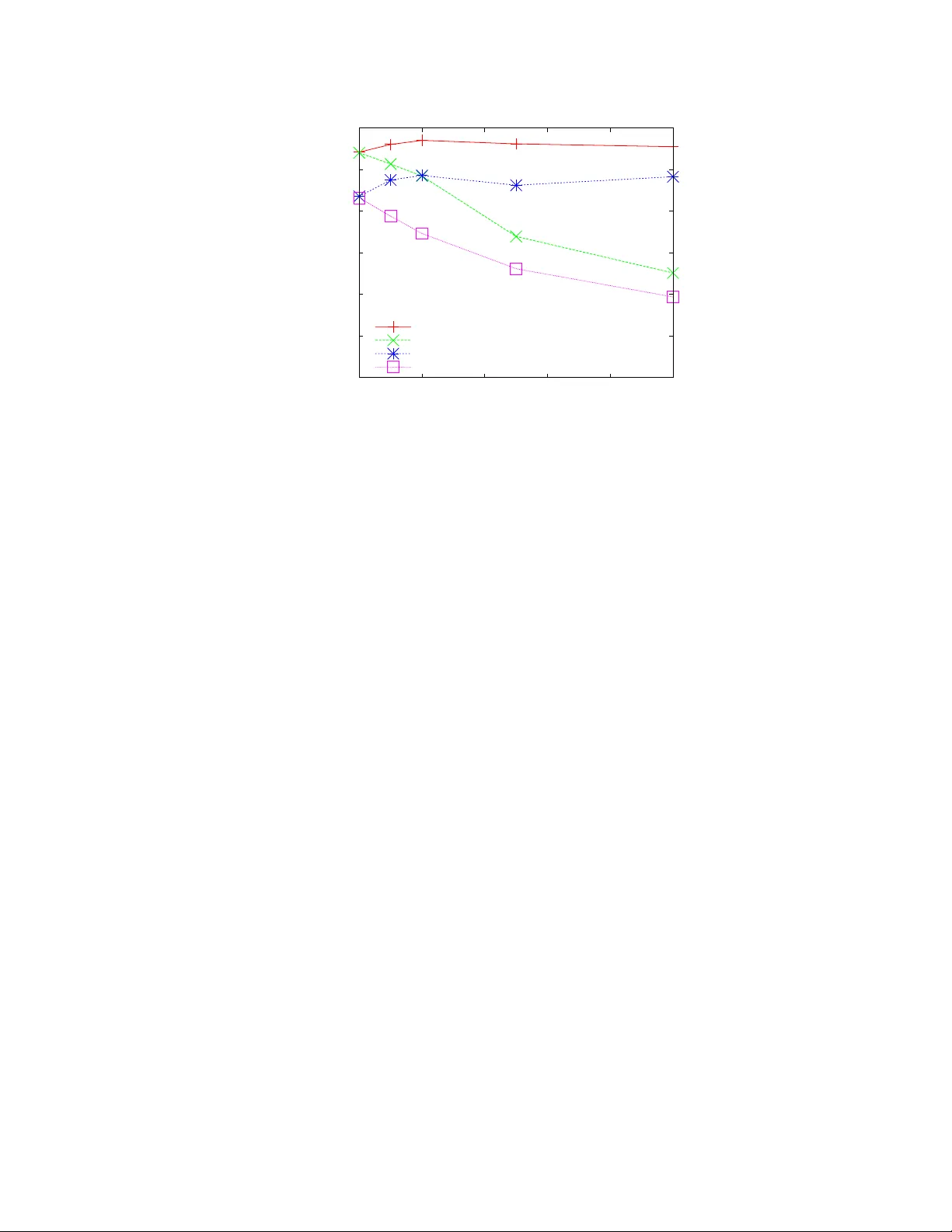
Stream sampling for v ariance-o ptimal estimation of subset sums ∗ Edith Cohen † Nick Duf field † Haim Kaplan ‡ Carsten Lund † Mikkel Thorup † Abstract From a high volume stream of weighted items, we want to maintain a gen eric sample of a certain limited size k th at we can later u se to estimate the total weight of arbitrary subsets. This is th e classic context of on-line reservoir sampling, thinking of the generic sample as a reservoir . W e present an effi- cient reservoir sampling scheme, V A R O P T k , that do minates all previous schemes in terms of estimation quality . V A R O P T k provides variance optimal unbiased estimation of subset sums . More precisely , if we have seen n items of the stream, then for an y subset size m , our scheme based on k samples minimizes the av er age v ar iance over all subsets o f size m . In fact, the optimality is against any off-line scheme with k samples tailored for the concrete set of items seen. In addition to o ptimal a verag e variance, our scheme provides tighter worst-case bound s on the variance o f particular subsets than p reviously possible. It is efficient, handling each ne w item of the stream in O (log k ) time. Finally , it is particularly well suited for combinatio n of samples from different s tr eams in a distributed setting. 1 Introd uction In this paper w e focus on sampling from a high volu m e stream of weighted items. T he items arriv e f aster and in lar ger quantities than can be sav ed, so only a sample can be stored ef ficiently . W e wa nt to maintain a generi c sample of a certain limited s ize that we can lat er use to es timate the total weight of arbit rary subs ets. This is a fund amental and pra ctical probl em. In [ 19] this is the basic functio n used in a data base system for streams. Such a sa m pling functio n is now inte grated in a measuremen t system for Internet traffic analys is [10]. In this conte xt, items are re cords su mm arizin g the flows of IP packe ts streamin g by a rou ter . Querie s on selecte d subsets ha ve numerous current and pote ntial applicati ons, in cluding anomaly detectio n (detecting unusu al traf fic pat terns by comparin g to h istoric data), traf fic e ngineering a nd rout ing (e.g., estimating traffic v olume between Aut onomous System (AS) pairs), and billing ( estimating vo lume of tra ffic to or from a certain sou rce or destination ). It is important that we ar e not constrain ed to subs ets kno wn in adv ance of the measuremen ts. This w ould preclude explo ratory studi es, and would not al low a chang e in routine questio ns to be applied retroacti vely to th e measu rements. A strikin g example where the selectio n is not kno wn in adv ance was the tracing of the Internet Slammer W orm [21]. It turned out to hav e a simple signatu re in the flow record; namely as bei ng udp traffic to port 1434 w ith a packet size of 404 bytes. Once this signa ture was iden tified, the worm could be studied by se lecting rec ords of flo ws matching this signature from th e sampled flow record s. W e introduce a new sampling and estimat ion s cheme for streams, denoted V A R O P T k , which selects k samples fr om n items. V A R O P T k has s eve ral importan t qualities: All es timates are unbiased . The s cheme is varian ce opti m al in th at it simultaneo usly minimizes the av erage vari ance of weight estimate s o ver su bsets of ∗ An extend ed abstract of this paper was presented at the 20th A CM-SIAM S ymposium on Discrete Algorithms, 200 9. † A T & T Labs—Research, Florham Park, NJ, USA (email: (edith,duffie ld,lund,mthor up)@research.att.com ) ‡ The Blav atnik School of Computer Science, T el A viv Uni versity , Israel (email: haimk@cs.t au.ac.il ) 1 e very size m < n . The a ver age vari ance optimal ity is comp lemented by optimal w ors t-case bound s limiting the v ariance o ver all combination s of input s treams an d qu eried subs ets. These p er-su bset worst -case boun ds are c ritical for appli cations requiring rob ustness and for th e deri vatio n of confidence interv als. Furthermor e, V A R O P T k is fast. It handles each item in O (log k ) worst-case time, and O (1) exp ected amortized time for randomly permute d streams. In Section 6 (Figure 1) we demon strate the estimation quality of V A R O P T k exp erimentally via a com- pariso n with other reserv oir sampling schemes on the Netflix Prize data set [23]. W ith our implementation of V A R O P T k , the time to sample 1,000 items from a stream of 10,000,00 0 items was only 7% slower than the time requir ed to read them. Ignori ng the on-line ef ficiency for st reams, there has been se ver al schemes prop osed that sati sfy the abo ve var iance properties both from statis tics [3, 33] and indirectly from computer science [28]. Here we formulate the sampling operatio n V A R O P T k as a genera l recurre nce, allo wing independe nt V A R O P T k samples from dif ferent subsets to be naturally combined to obtain a V A R O P T k sample of the entir e set. The schemes from [3, 33] fall out as specia l cases, and we get the fl exi bility needed for f ast on-line reserv oir sampling from a stream. The nat ure of the recu rrence is also perfect ly suited for distrib uted settin gs. Belo w we define the abov e qualiti es more pre cisely and pres ent an el aborate ov ervie w of pr eviou s work. 1.1 Reserv o ir sampling with unbiased estimation The problem we consider is classically kno wn as res ervoir sampling [20, pp. 138–14 0]. In reserv oir sam- pling, w e process a stream of (w eighte d) items. The items arri ve one at the time, and a reserv oir maintain s a sample S of the items seen thus far . When a new item arri ves, it may be included in the sample S and old items may be droppe d from S . Old items outside S are ne ver recon sidered. W e think of estimatio n as an integral part of sampling . Ultimately , we want to use a sample to estimate the total w eight of any subset of the items seen so far . F ixing notation, we are dealing with a stream of items where item i has a positi ve weight w i . For some inte ger capacity k ≥ 1 , we maintain a reserv oir S with capacit y for at most k samples from the items seen thus far . Let [ n ] = { 1 , . . . , n } be the set of items seen. W ith each item i ∈ S we store a w eight estimate b w i , w hich we also refer to as adjus ted weight . For items i ∈ [ n ] \ S w e hav e an implicit zero estimate b w i = 0 . W e require these estimators to be unb iased in the sense that E [ b w i ] = w i . A typical exa m ple is the classic Horvitz-Thomps on estimator [18] setting b w i = w i / Pr[ i ∈ S ] if i ∈ S . Our pur pose is to est imate arbitrary subs et sums from the sample. For any s ubset I ⊆ [ n ] , we l et w I and b w I denote P i ∈ I w i and P i ∈ I b w i , respecti vely . By linearity of expectat ion E [ b w I ] = w I . Since all unsampled items hav e 0 estimates, we get b w I ∩ S = b w I . Thus b w I ∩ S , the sum of the adjusted weights of items from the sample that are members of I , is an unbia sed estimator of w I . Reserv oir sampling thus addresses two issues: • T he streaming issue [22] w here w ith limited memory we want to compute a sample from a huge stream that passe s by only once. • T he incremental data structu re issue of maintaining a sample as ne w weigh ted items are inserted . In our case, we use the sample to prov ide quick estimates of sums over arbitrary subsets of the items seen thus far . Reserv oir versions of dif ferent samplin g schemes are presen ted in [4, 7, 12, 15, 13, 35]. 2 1.2 Off-line sampling When consideri ng the qualit ies of the sample, we compare our on-line scheme, V A R O P T k , with a powerfu l arbitra ry off-li ne sampling scheme which gets the n weighted items up front, and can tail or the sampling and estimation freely to this concret e set, not ha ving to worry about ef ficiency or the arriv al of more items. The only restriction is the b ound k on t he numbe r of sa mples. More abstractly , the of f-line sampl ing scheme is an arbitra ry probability distrib ution Ω over functions b w : [ n ] → R from items i to w eight estimates b w i which is unbia sed in the sense that E b w ← Ω [ b w i ] = w i , and which has at most k non-zeros. 1.3 Statistical pr o perties of target The sampling sch eme we want should sati sfy some clas sic goals from statistics. Belo w we describe these goals. Later we will di scuss their rele v ance to subset sum estimation. (i) Inclus ion pr obabili ties pr oportiona l to size (ipps) . T o get k samples , we wa nt each item i to be sample d with probability p i = k w i /w [ n ] . This is not possible if some item j has more than a fraction k of the total weight. In that case, the standar d is that w e include j with probability p j = 1 , and recursi vely ipps sample k − 1 of the remaining items. In the special case where w e start with k ≥ n , we end up including all items in the sample. The inc luded items are gi ven the standa rd Horvitz-Thompso n estimate b w i = 1 /p i . Note that ipps only conside rs the margina l distrib ution on each item, so many joint distrib utions are possib le and in itself, it only leads to an expect ed number of k items. (ii) Sample contain s at most k items . Note that (i) and (i i) tog ether implies that the s ample con tains exac tly min { k , n } items. (iii) No posit ive covar iances between distin ct adjusted weights. From statistics, we kno w se veral schemes satisfying the abov e goals (see, e.g., [3, 33 ]), but they are not ef ficient for on-line reserv oir sampling. In addition to the ab ove goa ls, we will s how tha t V A R O P T k estimates admit standa rd Chernof f bounds. 1.4 A verage variance optimal ity Belo w we will discuss some a verage var iance measures that are automatica lly optimized by goal (i) and (ii) abo ve. When n items ha ve arri ved , for each subset size m ≤ n , we consid er the av erage varia nce for subsets of size m ≤ n : V m = E I ⊆ [ n ] , | I | = m [ V ar [ b w I ]] = P I ⊆ [ n ] , | I | = m [ V ar [ b w I ]] n m . Our V A R O P T k scheme is vari ance opt imal in the follo w ing stron g sense. For each reserv oir size k , stream prefix of n weighted items, and subset size m , there is no of f-line sampling scheme with k sampl es getting a smaller a verage varia nce V m than our gener ic V A R O P T k . The a verage va riance measure V m was int roduced in [30] where it was pro ved that V m = m n n − m n − 1 Σ V + m − 1 n − 1 V Σ , (1) 3 Here Σ V is the sum of indi vidual vari ances while V Σ is the v ariance of the estimate of the total, that is, Σ V = X i ∈ [ n ] V ar [ b w i ] = nV 1 V Σ = Va r [ X i ∈ [ n ] b w i ] = V ar [ b w [ n ] ] = V n . It follo ws that we minimize V m for all m if and only if we simultane ously minimize Σ V and V Σ , w hich is exa ctly w hat V A R O P T k does. The optimal val ue for V Σ is 0 , meaning that the es timate of the total is exa ct. Let W p denote the expecte d varian ce of a random subset in cluding each item i independ ently with so m e probab ility p . It is also sh own in [3 0 ] tha t W p = p ((1 − p )Σ V + pV Σ ) . S o i f w e simultaneousl y minimize Σ V and V Σ , w e also minimize W p . It should be noted that both Σ V and V Σ are kno wn measures from statist ics (see , e.g., [27] and con crete examples in the ne xt section). It is the implicatio ns for a verag e v ariance ov er subsets that are from [30]. W ith no informati on giv en about which kind of subsets are to be estimated, it makes m ost sense to optimize av erage v ariance measures like those abov e giving each item equal opp ortunity to be includ ed in the estimat ed subset. If the inp ut distrib utions are not too specia l, then we exp ect this to gi ve us the bes t estimates in practice , using v ariance as the classic measure for estimation quality . Related auxiliary var iables W e no w consider the case where we for each item are interested in an auxil- iary weight w ′ i . For these we use the estimate b w ′ i = w ′ i b w i /w i , which is unbiased since b w i is unbiased. Let V Σ ′ = P i ∈ [ n ] b w ′ i be the v ariance on the estimate of the total for the auxiliary variab les. W e will argu e that w e expect to do best possible on V Σ ′ using V A R O P T k , assuming that the w ′ i are randomly generated from the w i . Formally we assume each w ′ i is generated as w ′ i = x i w i where the x i are dra w n independ ently from the same distrib ution Ξ . W e consider expect ations E Ξ for random choices of the vec tor x = ( x i ) i ∈ [ n ] , that is, formall y E Ξ [ V Σ ′ ] = E x ← Ξ n [ V Σ ′ | x ] . W e will prov e E Ξ [ V Σ ′ ] = Va r [Ξ]Σ V + E [Ξ] 2 V Σ , (2) where V ar [Ξ] = Va r Ξ [ x i ] and E [Ξ] = E Ξ [ x i ] for eve ry x i . From (2) it follo ws that we minimize E Ξ [ V Σ ′ ] when we simultan eously minimize Σ V and V Σ as we do with V A R O P T k . Note that if the x i are 0/1 v ariables, then the b w ′ i repres ent a random sub set, includin g each item independ ently as in W p abo ve. The proof of (2) is found in Append ix A Relation to statistics The abov e auxiliary v ariables can be though t of as modeling a classic scenari o in statistics, found in text books such as [27]. W e are interested in some w eights w ′ i that will only be re vealed for sampled items. Ho wev er , for e very i , we ha ve a kno wn approximat ion w i that we can use in decidi ng which items to sample. As an example , the w ′ i could be household incomes while the w ′ i where approx imations bas ed on postal codes. The m ain purpose of the sampling is to estimate the total of the w ′ i . When e v aluating dif ferent schemes, [27] consider s V Σ , sta ting that if the w ′ i are p roportional to the w i , th en the va riance V Σ ′ on the estimated total P i b w ′ i is proportio nal to V Σ , and therefo re we should minimize V Σ . This correspond s to the case w here Va r [Ξ] = 0 in (2). Howe ver , (2 ) shows that Σ V is also important to V Σ ′ if the relatio n between w ′ i and w i is not just propo rtional, bu t also has a random component. As st ated, Σ V is not normally the foc us in statistics , bu t for Poisson samp ling w here each item is sa m pled indepe ndently , we ha ve Σ V = V Σ , and study ing this case, it is sho wn in [27, p. 86] that the ipps of goal (i) uniqu ely minimizes Σ V (see [12] for a proof work ing directly on the general case allowin g dominant 4 items). It is also easy to verif y that condition ed on (i), goal (ii) is equiv alent to V Σ = 0 (again this appears to be stan dard, but we couldn’ t find a reference for the general state ment. The arg ument is tri vial thoug h. Giv en the (i), the only v ariability in the weight estimates returned is in the number of sampled estimates of v alue τ , so the estimate of the total is varia ble if and only if the number of samples is varia ble). The classic goals (i) and (ii) are thus equi val ent to minimizing Σ V and V Σ , hence all the av erage varian ces discuss ed abo ve. 1.5 W orst-case r obustness In additio n to minimizing the a verage var iance, V A R O P T k has some complimen tary worst- case rob ustness proper ties, limiting th e var iance for eve ry sing le (arbitrary) sub set. W e no te that any su ch bound has to gro w with the square of a scaling of the weights. This kind of rob ustness is importan t for application s seekin g to minimize worst-ca se vu lnerability . The robust ness dis cussed below is all a conseq uence of the ipps of goal (i) combined with the non-p ositiv e cov ariances of goal (iii). W ith the H orvitz -T hompson estimate, the va riance of item i is w 2 i (1 /p i − 1) . W ith ipps sampling, p i ≥ min { 1 , k w i /w [ n ] } . This gi ves us the two bounds V ar [ b w i ] < w i w [ n ] /k and Va r [ b w i ] < ( w [ n ] / (2 k )) 2 (for the second bound note that p i < 1 implies w i < w [ n ] /k ). Both of these bound s are asymptoti cally tight in that sense that there are instanc es for which no sampling scheme can get a better leading const ant. More precis ely , the bound Va r [ b w i ] < w i w [ n ] /k is asymptoticall y tight if ev ery i has w i = o ( w [ n ] /k ) , e.g., when sampling k out of n units, the indiv idual v ariance we get is ( n/k ) − 1 . The bound ( w [ n ] / (2 k )) 2 is tight for n = 2 k unit items. In combinatio n with the non-p ositiv e cov ariance s of goal (iii), we get that e very subset I has w eight- bounded vari ance Va r [ b w I ] ≤ w I w [ n ] /k , and cardin ality bounded v ariance V ar [ b w I ] ≤ | I | ( w [ n ] / 2 k ) 2 . 1.6 Efficient for each item W ith V A R O P T k we can handle each new item of the stream in O (log k ) worst-case time. In a realisti c implementa tion w ith floatin g point numbers, we ha ve some p recision ℘ and acc ept an error of 2 − ℘ . W e will pro ve an Ω(log k / log log k ) lo wer bound on the worst -case time for processi ng an item on the word RAM for any floating point implementat ion of a reserv oir sampling scheme w ith capacity for k samples which satisfies goal (i) minimizing Σ V . Complementing that we will sho w tha t it is possible to handle each item in O (log log k ) amortize d time. If the stream is viewed as a ran dom permutat ion of the items, we will sho w that the exp ected amortized cost per item is only constant. 1.7 Known sampling schemes W e will no w discuss known sampli ng schemes in relati on to the qualitie s of our new pro posed scheme: • A ve rage varian ce optimali ty of Section 1.4 follo wing from goal (i) and (ii). • T he rob ustness of S ection 1.5 fol lowing from goal (i) and (iii). • E f fi cient reserv oir sampling implementation with capacity for at most k samples; efficien t distri buted implementa tion. The statis tics literature c ontains many sampling schemes [27, 34] t hat share some of these qualities, b ut the n the y all perform significantly worse on others. 5 Unifo rm sampling without replacement In uniform sampling without replacement, we pick a sample of k items uniformly at random. If item i is sampled it gets the Horvi tz-Thompson weight est imate b w i = w i n/k . Uniform sampling has obvi ous v ariance problems with the frequ ently-occurr i ng heavy -tailed po wer- lo w distri bution s, where a small fraction of dominan t items account s for a large fraction of the total w eight [1, 25], becaus e it is likely to miss the dominant items. Pro b ability pro p ortional to size sampling with replac ement (ppswr) In probabil ity propo rtional to size sampling (pps) w ith replacement (wr), each sample S j ∈ [ n ] , j ∈ [ k ] , is ind ependent, and equ al to i with probabili ty w i /w [ n ] . T hen i is sampled if i = S j for some j ∈ [ k ] . This happens w ith probabi lity p i = 1 − (1 − w i /w [ n ] ) k , and if i is sampled, it gets the Horvitz-Thomps on estimator b w i = w i /p i . Other estimato rs hav e bee n propos ed, but we always ha ve the same problem with heavy -tailed distrib utions: if a fe w dominant items conta in most of the total weight , then m ost samples will be copie s of these dominan t items. A s a result, we are left with comparati vely fe w samples of the remaining items, and few samples imply high v ariance no matter which estimates we assign. Pro b ability propor tional to size sampling w ithout r eplacement (pp swor) An ob vious improve ment to ppswr is to sample without repl acement (ppswor). Each new item is then chosen with probab ility propor - tional to size among the items not yet in the sample. W ith ppswo r , unlik e ppswr , the probab ility that an item is included in the sample is a complicat ed function of all the item weights, and therefore the Horvitz- Thompson estimator is not directly app licable. A ppsw or reserv oir sampling and est imation procedur e is, ho wev er , presented in [7, 6, 8]. Even though p pswor resolv es the “du plicates proble m ” of pp swr , we claim here a negat ive result for any ppswo r estimator: in Appendi x B, we will present an instance for any sample size k and number of items n such that any estimation based on up to k + (ln k ) / 2 ppsw or samples will perfor m a factor Ω(log k ) worse than V A R O P T k for every subset size m . This is the first such negati ve result for the classic ppswor besides the fact that it is not strict ly optimal. Ipps Poisson sampling It is more con ven ient to think of ipps sampling in terms of a thr eshold τ . W e includ e in the sample S ev ery item with weight w i ≥ τ , using the original weight as estimate b w i = w i . A n item i with weight w i < τ is includ ed with probabil ity p i = w i /τ , and it gets weigh t estimate τ if sampled. For an e xpected number of k < n samples, we use the unique τ = τ k satisfy ing X i p i = X i min { 1 , w i /τ k } = k . (3) For k ≥ n , we define τ k = 0 which implies that all items are included. This thresho ld centric vie w of ipps sampling is tak en from [11]. If the thresho ld τ is giv en, and if we are satisfied with P oisson sampling, that is, each item is sampled indepe ndently , then we can trivial ly perform the sampling from a stream. In [12] it is sho wn ho w we can adjust the threshol d as samples arriv e to that we always ha ve a reserv oir with an expe cted number of k samples, sa tisfying goal (i) for t he items seen thus f ar . Note, ho weve r , that we may e asily violate goal (ii) of ha ving at most k samples. Since the items are sampled indep endently , we ha ve zero cov ariances, so (iii) is satisfied along with the all th e robus tness of Section 1.5. Howe ver , the av erage v ariance of Sectio n 1.4 suf fers. More preci sely , with zero cov ariances, we get V Σ = Σ V instead of V Σ = 0 . From (1) w e get that for subset s of size m , the 6 a verage var iance is a fa ctor ( n − 1) / ( n − m ) larg er than for a scheme satisf ying both (i) and (ii). Similarly we get that the a verage varia nce W 1 2 ov er all subsets is large r by a factor 2. Priority sampling Prior ity s ampling was introdu ced in [12] as a thresho ld centr ic sc heme whi ch is tailored for reser voir sampling w ith k as a hard capacit y const raint as in (ii). It is pro ved in [29] that priority sampling with k + 1 samples gets as g ood Σ V as the op timum obtained by (i) with only k samples . P riority sampl ing has zero cov arianc es like the abo ve ipps P oisson sampl ing, so it satisfies (iii), b ut with V Σ = Σ V it has the same lar ge av erage v ariance for large r subsets . Satisfying the goals but not w ith efficient res ervoi r sampling As noted previ ously , there are se veral schemes satisfyin g all our goal s [3, 33, 28], b ut the y are not efficient for reserv oir sampling or distrib uted data. Chao’ s scheme [3] can be seen as a reserv oir sampling scheme, bu t when a ne w item arri ves, it compute s all the ipps proba bilities from scratc h in O ( n ) time, leadin g to O ( n 2 ) total time. Till ´ e [33] has of f-line scheme that eliminates items from possibly being in the sample one by one (Till ´ e also consid ers a complement ary scheme that draws the samples one by one). Each elimination step in v olves computing eliminati on probabil ities for each remaining item. As such , he ends up spend ing O (( n − k ) n ) time ( O ( k n ) for th e compleme ntary scheme) on selecting k samples. Srini vasan [28] has presented the most ef ficient of f- line scheme, b ut cast for a diffe rent problem. His input are the desired inclusion probabilit ies p i that should sum to k . H e then selects the k samples in linear time by a simple pairin g pro cedure that can ev en be used on-lin e. Howe ver , to apply his algorithm to our problem, we first need to compute the ipps probabilit ies p i , and to do that, w e first need to know all the w eights w i , turning the w hole thing into an off-l ine linear time algori thm. Srini vasan states that he is not aw are of any pre vious scheme t hat can s olve his task, b ut u sing his inclus ion probabil ities, the abo ve mentioned older schemes from sta tistics [3, 33] will do the job , albeit less ef ficiently . W e shall discuss our technical relation to [3, 33] in more detail in Section 2.3. O ur contrib ution is a scheme V A R O P T k that satisfies all our goals (i)–(iii) while being efficient reserv oir sampling from a stream, proces sing each new item in O (log k ) time. 1.8 Contents In Section 2 we will present our recurre nce to generate V A R O P T k schemes, including those from [3, 33] as spe cial cases. In S ection 3 we will prove that the general method works. In Section 4 we will pre sent ef ficient implementa tions, complement ed in Section 5 with a lower bound. In Section 6 we present an exp eriment compariso n with other sampling and estimatio n scheme. Finally , in Section 7 w e prove that our V A R O P T k schemes actual ly admit the kind of Chernof f bounds we usually associate with independ ent Poisson samples. 2 V A R O P T k By V A R O P T k we w ill refer to any unbiased sampling and estimati on scheme satis fying our goals (i)–(iii) that we recall belo w . (i) Ipps. In the rest of the paper , we use the threshold centric definition from [11] mentioned under ipps Poisson sa mpling in Sec tion 1.7. Thus we hav e the s ampling probabili ties p i = m in { 1 , w i /τ k } w here τ k is the unique valu e such that P i ∈ [ n ] min { 1 , w i /τ k } = k assuming k < n ; otherwis e τ k = 0 meaning that all items are sampled. T he expected number of samples is thus min { k , n } . A sampled 7 item i gets the Horvitz-Thomps on estimator w i /p i = m ax { w i , τ k } . W e refe r to τ k as the thr eshold when k and the weights are under stood. (ii) At most k samples. T ogether with (i) this means exactl y min { k , n } samples. (iii) No positi ve cov ariance s. Recall that these propert ies imply all v ariance qualities mentioned in the introdu ction. As mentione d in the introd uction, a clean design that diffe rentiates our V A R O P T k scheme from preced - ing schemes is that we can just sample from sample s without rely ing on auxiliary data. T o m ake sense of this statemen t, we let all samplin g scheme operate o n some adj usted weights, which i nitially are the origina l weights. When we sample some items w ith adjusted weight, we use the resulting w eight estimates as new adjust ed weights, treating them exactl y as if they were ori ginal weights. 2.1 A general r ecurren ce Our main contrib ution is a general recurrenc e for genera ting V A R O P T k schemes. Let I 1 , ..., I m be disjoint non-emp ty sets of weighted items, and k 1 , ..., k m be inte gers each at least as large as k . Then V A R O P T k ( [ x ∈ [ m ] I x ) = V A R O P T k ( [ x ∈ [ m ] V A R O P T k x ( I x )) (4) W e refer to the calls to V A R O P T k x on the right hand side as the inner subcalls , the call to V A R O P T k as the outer subcall . T he call to V A R O P T k on the left hand side is the r esulting call . The recurrenc e states that if all the sub calls are V A R O P T k schemes (with the k x replac ing k for the inner subcall s), that is, unbia sed sampling and estimation schemes satisfy ing proper ties (i)–(iii), then the resu lting call is also a V A R O P T k scheme. Here we assu me that the rando m choice s of dif ferent subca lls are indepe ndent of each other . 2.2 Specializing to r eservoir sampling T o make use of (4) in a streamin g conte xt, first as a ba se ca se, we assume an implement ation of V A R O P T k ( I ) when I has k + 1 items, denoting this proced ure V A R O P T k ,k +1 . This is very simple and has been done befor e in [3, 33]. Specia lizing (5) with m = 2 , k 1 = k 2 = k , I 1 = { 1 , ..., n − 1 } and I 2 = { n } , we get V A R O P T k ([ n ]) = V A R O P T k ,k +1 ( V A R O P T k ([ n − 1]) ∪ { n } ) . (5) W ith (5) we immediately get a V A R O P T k reserv oir sampling algorithm: the first k items fi ll the initial reserv oir . Thereafter , whenev er a ne w item arriv es, we add i t to the current res ervoir s ample, which becomes of size k + 1 . Finally w e apply V A R O P T k ,k +1 sample to the result. In the application of V A R O P T k ,k +1 we do not disting uish between items from the pre vious reserv oir and the new item. 2.3 Relation to Chao’ s and T i ll ´ e’ s pr ocedures When we use (5), we generate exac tly the same distrib ution on samples as that of C hao’ s procedure [3]. Ho w e ver , C hao does not use adju sted weights, let alone the general recur rence. Instea d, when a new item n arri ves, he computes the ne w ipps probabili ties using the recursi ve formula from statics m ention ed under (i) in S ection 1.3. This formula tion may in vo lve details of all the original weights e ven if we are only want the inclu sion probability of a gi ven item. C omparing the new and the prev ious probabil ities, he fi nds the 8 distrib ution for which item to drop. Our recurrence with adjusted weights is simpler and more ef fi cient becaus e w e can forg et about the past: the original weights and the inclusio n probab ilities from previo us round s. W e can also use (4) to deri ve the eliminatio n procedur e of Till ´ e [33]. T o do that, w e set m = 1 and k 1 = k + 1 , yielding the recurrence V A R O P T k ( I ) = V A R O P T k ,k +1 ( V A R O P T k +1 ( I )) This tells us how to draw k samples by eliminating the n − k other items one at the time. L ike Chao, Till ´ e [33] computes the elimin ation probabi lities for al l items in all ro unds direc tly from the o riginal weights . Our genera l recurren ce (4) based on adjusted weights is more fl exi ble, simpler , and more efficient. 2.4 Relation to pr evious reser voir sampling schemes It is easy to see that nothing like (5 ) works for any of the other reserv oir sampling schemes from the intro- ductio n. E.g., if U N I F k denote s uniform sampling of k items with associat ed estimates, then U N I F k ([ n ] } ) 6 = U N I F k ,k +1 ( U N I F k ([ n − 1]) ∪ { n } ) . W ith equality , this formula would say that item n shoul d be included with probabil ity k / ( k + 1) . Howe ver , to integ rate item n correctl y in the unifo rm reserv oir sample, we sho uld only include it with probab ility k /n . The standa rd algorithms [15, 35] therefore maintain the index n of the last arri val. W e hav e the same issue with all the other schemes: ppswr , ppswor , priority , and P oisson ipps samplin g. For each of these schemes, we ha ve a global descriptio n of what the rese rvoir should look like for a giv en stream. When a ne w item arri ves, w e cannot just treat it like the current items in the reserv oir , sampling k out of the k + 1 items. Instead we need some additional information in order to integrat e the ne w ite m in a va lid reserv oir sample of the new exp anded stream. In particu lar , priority sampling [12] and the ppswor schemes of [7, 6, 8] use prio rities/ranks for all items in the reserv oir , and the reserv oir vers ion of Poisso n ipps samplin g from [11, 12] uses the sum of all weights belo w the current threshold. Generalizing from unit weights The standa rd scheme [15, 35] for sampling k unit items is varian ce optimal and w e can see V A R O P T k as a generali zation to weighted items which produces ex actly the same sample and estimat e distrib ution when applie d to unit weights. T he standard scheme for unit items is, of course , much simple r: we inclu de the n th item with probability n /k , pushing out a uni formly random old one. The estimate of any sampled item becomes n/k . W ith V A R O P T k , when the n th item arriv es, we ha ve k old adjuste d weights of size ( n − 1) /k and a ne w item of w eight 1 . W e apply the general V A R O P T k ,k +1 to get down to k weights. The result of this more con v oluted proc edure ends up the same: the ne w item is includ ed with probabi lity 1 /n , and all adjusted weights become n/k . Ho w e ver , V A R O P T k is not the only natural generaliz ation of the standard scheme for unit w eights . T he ppswo r schemes from [7, 6 , 8] also produce t he same results when applied to uni t weigh ts. Howe ver , ppswor and V A R O P T k di ver ge w hen the weight s are not all the same. The pps wor scheme from [8] does hav e exact total ( V Σ = 0 ), b ut suboptimal Σ V so it is not varia nce optimal . Priority sampling is also a generalizati on in that it produces the same sample distrib ution w hen applied to unit weights. Howe ver , the estimates vary a bit, and that is why it only optimizes Σ V modulo one extra sample. A bigger cav eat is that priority sampling does not get the total exact as it has V Σ = Σ V . The V A R O P T k scheme is the unique genera lization of the sta ndard reserv oir sampling sche m e for unit weights to genera l weights that preserv es va riance optimality . 9 2.5 Distribu ted and parallel settings Contrast ing the abov e specializat ion for streams, we note that the general recurren ce is useful in, say , a distrib uted setting, where the sets I x are at dif ferent locations and only local samples V A R O P T k x ( I x ) are forwar ded to the tak e part in the glob al sample. Like wise, we ca n use the general recurr ence for fast parallel computa tion, cutting a huge file I into segments I x that we sample from indepen dently . 3 The recurr ence W e will no w establish the recurrence (4) stating that V A R O P T k ( [ x ∈ [ m ] I x ) = V A R O P T k ( [ x ∈ [ m ] V A R O P T k x ( I x )) Here I 1 , ..., I m are disj oint non-empty sets of weighted items, and we ha ve k x ≥ k for each x ∈ [ m ] . W e wa nt to sho w that if each sub call on the right hand side is a V A R O P T k scheme (with the k x replac ing k for the inner subcal ls), that is, unbias ed sampling and estimatio n schemes satisfying (i)–(iii), then the resulti ng call is also a V A R O P T k scheme. The hardest part is to prov e (i), and w e will do tha t last. Since an unbiased esti m ator of an unbias ed estimator is an unbia sed estimator , it follo ws that (4) pre- serv es unbiasedn ess. For (ii) we just nee d to ar gue that the resulting sample is of size at most k , and that follo ws trivia lly from (ii) on the outer subcall, regar dless of the inner subcalls. Before provin g (i) and (iii), we fix some notation. Let I = S x ∈ [ m ] I x . W e use w i to denote the original weights. For each x ∈ [ m ] , set I ′ x = V A R O P T k ( I x ) , and use w ′ i for the resulti ng adjuste d weights. Set I ′ = S x ∈ [ m ] I ′ x . Finally , set S = V A R O P T k ( I ′ ) and use the fi nal adjusted weights as weight estimates b w i . Let τ x,k x be the thres hold used in V A R O P T k ( I x ) , and let τ ′ k be the thres hold used by V A R O P T k ( I ′ ) . Lemma 1 The r ecurr ence (4) pr eserves (iii). Pro of Wi th (iii) is satisfied for each inner subca ll, we know that there are no positi ve cov ariances in the adjuste d weights w ′ i from I ′ x = V A R O P T k ( I x ) . Since these samples are indepe ndent, we get no positi ve cov arianc es in w ′ i of all i tems in I ′ = S x ∈ [ m ] I ′ x . Let ( I 0 , w 0 ) denote a ny p ossible concr ete valu e of ( I ′ , w ′ ) . Then E [ b w i b w j ] = X ( I 0 ,w 0 ) Pr[( I ′ , w ′ ) = ( I 0 , w 0 )] · E [ b w i b w j | ( I ′ , w ′ ) = ( I 0 , w 0 )] ≤ X ( I 0 ,w 0 ) Pr[( I ′ , w ′ ) = ( I 0 , w 0 )] w 0 i w 0 j = E [ w ′ i w ′ j ] ≤ w i w j . T o deal with (i), we need the follo wing general consequenc e of (i) and (ii): Lemma 2 If (i) and (ii) is satisfied by a scheme sampling k out of n items, then the multiset of adjusted weight value s in the sample is a unique functio n of the input weights. 10 Pro of If k ≥ n , we include all weights, and the result is tri vial, so we may assume k < n . W e already noted that (i) and (ii) imply that exactly k items are sampled . The threshold τ k from (3) is a function of the input weights. All items with higher weights are included as is in the sample, and the remain ing sampled items all get adjus ted weight τ k . In the rest of this section, w e assume that each inner subcall satisfi es (i) and (ii), and that the outer subcall satisfi es (i) . Based on these assu mptions, we will sho w that (i) is satisfied by the resulting call. Lemma 3 The thr eshold τ ′ k of the outer sub call is unique . Pro of W e appl y Lemma 2 to all the inner subca lls, and conclud e that the multiset of adjusted w eight v alues in I ′ is uniqu e. This multiset uniqu ely determines τ ′ k . W e no w consider a simple degenera te cases. Lemma 4 The r esulting call satisfi es (i) if | I ′ | = P x ∈ [ m ] | I ′ x | ≤ k . Pro of If | I | = P x ∈ [ m ] | I x | ≤ k , there is no acti ve sampling by any call, and then (i) is trivia l. Thus we may assume P x ∈ [ m ] | I ′ x | = P x ∈ [ m ] min { k x , | I x |} ≤ k < P x ∈ [ m ] | I | . This implies that | I ′ x | = k x ≥ k for some x . W e conclud e that m = 1 , x = 1 , and k 1 = k , and this is independe nt of random choice s. The resulti ng sample is then is identi cal to that of the single inner subcall on I 1 and we hav e assumed that (i) holds for this call. In the rest of the proof, we assume | I ′ | > k . Lemma 5 W e hav e that τ ′ k > τ x,k x for each x ∈ [ m ] . Pro of S ince we ha ve assumed | I ′ | > k , we ha ve τ ′ k > 0 . The statemen t is thus trivi al for x if | I x | ≤ k implying τ x,k x = 0 . Howe ver , if | I x | ≥ k , then from (i) and (ii) on the inner sub call V A R O P T k x ( I x ) , we get that the returned I ′ x has ex actly k x items, each of weight at least τ x,k x . These items are all in I ′ . Since | I ′ | > k , it follo ws from (i) with (3) on the outer subc all that τ ′ k > τ x,k x . Lemma 6 The res ulting sample S includes all i with w i > τ ′ k . Mor eover , each i ∈ S has b w i = max { w i , τ ′ k } . Pro of S ince τ ′ k > τ x,k x and (i) holds for each inner subcall, it follo ws that i ∈ I has w ′ i = w i > τ ′ k if and only if w i > τ ′ k . The result no w follo w s from (i) on the outer subcall. Lemma 7 The pr oba bility that i ∈ S is p i = m in { 1 , w i /τ ′ k } . Pro of F rom L emma 3 and 6 we get that b w i equals the fixed value m ax { w i , τ ′ k } if i is sampled. Since b w i is unbia sed, we conclude that p i = w i / max { w i , τ ′ k } = min { 1 , w i /τ ′ k } . Lemma 8 τ ′ k is equa l to the thr eshold τ k define d dir ectly for I by (i). 11 Pro of S ince the input I ′ to the outer subcall is more than k items and the call satisfies (i), it returns an expec ted number of k items and these form the fi nal sample S . W ith p i the probability that item i is includ ed in S , we conclude that P p i = k . Hence by L emma 7 , we ha ve P i min { 1 , w i /τ ′ k } = k . Howe ver , (i) defines τ k as the uniqu e v alue such that P i min { 1 , w i /τ k } = k , so we conclude that τ ′ k = τ k . From Lemma 6, 7, and 8, we conclud e Lemma 9 If (i) and (ii) are satisfi ed for eac h inner subcall and (i) is satisfied by the outer subca ll, then (i) is satis fied by the r esulting call. W e hav e no w sho wn that the sampl e S w e generate satis fi es (i), (ii), and (iii), hence that it is a V A R O P T k sample. T hus (4) follo ws. 4 Efficient implementations W e will no w sho w how to imp lement V A R O P T k ,k +1 . First we giv e a basic implementa tion equi val ent to the one used in [3, 33]. L ater we will tune our implementa tion for use on a stream. The inp ut is a set I of n = k + 1 items i with adjusted weights ˜ w i . W e want a V A R O P T k sample of I . First we compute the thre shold τ k such that P i ∈ [ n ] min { 1 , ˜ w i /τ k } = k . W e want to include i with probability p i = m in { 1 , ˜ w i /τ k } , o r equi vale ntly , to dro p i with p robability q i = 1 − p i . Here P i ∈ I q i = n − k = 1 . W e partiti on the unit interv al [0 , 1] into a segment of size q i for each i with q i > 0 . F inally , we pick a random point r ∈ [0 , 1] . T his hits the interv al of some d ∈ I , and then w e drop d , setti ng S = I \ { d } . For each i ∈ S with ˜ w i < τ k , we set ˜ w i = τ k . Finall y w e return S with th ese adjus ted weights . Lemma 10 V A R O P T k ,k +1 is a V A R O P T k sch eme. Pro of It follows direct ly from the definition that we use thre shold probabiliti es and estimators, so (i) is satisfied. S ince we drop one, we end up with exactly k so (ii) follo ws. F inally , we need to argue that there are no positi ve cov ariances. W e coul d only hav e positi ve cov ariances between items below the thresho ld whose inclus ion probability is belo w 1 . Knowing that one such item is includ ed can only decrease the chance that anoth er is includ ed. Since the alw ays get the same estimate τ k if inclu ded, we conclu de that the cov arianc e between these items is negati ve. This set tles (iii). 4.1 An O (log k ) implementation W e will no w improv e V A R O P T k ,k +1 to handle each new item in O (log k ) time. Instea d of starting from scratch , we want to mai ntain a reserv oir w ith a s ample R of size k for the items seen thus f ar . W e denote by R j the a reserv oir after processing item j . In the next subsection, we will sho w ho w to process each item in O (1) expecte d amortized time if the input stream is rando m ly permuted. Consider round j > k . Our first goal is to identify the new threshol d τ = τ k ,j > τ k ,j − 1 . Then w e subsamp le k out of the k + 1 items in R pre j = R j − 1 ∪ { j } . Let ˜ w (1) , ..., ˜ w ( k +1) be the adjuste d weights of the items in R pre j in increasing sorted order , breakin g ties arbitr arily . W e first identi fy the larges t number t 12 such that ˜ w ( t ) ≤ τ . Here ˜ w ( t ) ≤ τ ⇐ ⇒ k + 1 − t + ( X x ≤ t ˜ w ( x ) ) / ˜ w ( t ) ≥ k ⇐ ⇒ ( X x ≤ t ˜ w ( x ) ) / ˜ w ( t ) ≥ t − 1 . (6) After finding t we fi nd τ as the solution to ( X x ≤ t ˜ w ( x ) ) /τ = t − 1 ⇐ ⇒ τ = ( X x ≤ t ˜ w ( x ) ) / ( t − 1) . (7) T o find the item to lea ve out, we pick a uniformly random number r ∈ (0 , 1) , and find the smallest d ≤ t such that X x ≤ d (1 − ˜ w ( x ) /τ ) ≥ r ⇐ ⇒ dτ − X x ≤ d ˜ w ( x ) ≥ rτ . (8) Then the d th smallest item in R pre j , is the one we drop to create the sample S = R j . The equa tions abov e sugges ts that we find t , τ , and d by a binary searc h. When w e cons ider an item during this search we need to kno w the number of items of smaller adjusted weight, and their total adjusted weight. T o perfo rm this binary search we represent R j − 1 di vided into two sets. The set L of lar ge items with w i > τ k ,j − 1 and ˜ w i = w i , and the set T = R j − 1 \ L of small items whose adjusted weight is equal to the thresh old τ k ,j − 1 . W e represen t L in sorted order by a balance d binary search tree. Each nod e in this tree stores the number of items in its subtre e and their total weight. W e repr esent T in sorted order (here in fact the order cou ld be arbitrary) by a b alanced binary search tree , where ea ch node in this tree sto res the number of items in its subtree. If w e multiply the number of items in a subtree of T by τ k ,j − 1 we get their total adjust ed weight. The heigh t of each of the se two trees is O (log k ) so we can i nsert or d elete an element, or concatenat e or split a lis t in O (log k ) time [9]. Furthermore, if we follo w a path do wn from the ro ot of one of these tree s to a node v , then by accumulating counte rs from roots of subtrees hanging to the left of the path, and smaller nodes on the path, we can maintain the number of items in the tree smaller than the one at v , and the total adjust ed weight of these items. W e process ite m j as f ollows. If it em j is larg e, that is w j > τ k ,j − 1 , w e insert i t into the tree re presenting L . Then we find t by searching the tree over L as follows. While at a node v we compute the total number of items smalle r than th e one at v by adding to the n umber of such items in L , | T | or | T | + 1 depend ing upon whether w j ≤ τ k ,j − 1 or not. S imilarly , we compute the total adjust ed w eight of items smaller than the one at v by adding | T | τ k ,j − 1 to the total w eight of such items L , and w j if w j ≤ τ k ,j − 1 . Then we use Equatio n (6) to decide if t is th e index of the ite m at v , or we sh ould proceed to the left or to the ri ght child of v . After computin g t we compute τ by Equation (7). Next w e identify d by first considerin g item j if w j < τ k ,j − 1 , and t hen search ing either the tree o ver T or the tree o ver L in a way similar to the se arch for c omputing t but using Equation (8). Once findi ng d our subsample becomes R j = S = R pre j \ { d } . All this takes O (log k ) . Last we upda te our rep resentation o f the reserv oir , so that it corre sponds to R j and τ k ,j . W e insert w j into T if w j ≤ τ k ,j − 1 (other w ise it had already been inserte d into L ). W e also delete d from the list containing it. If w ( t ) was a lar ge w eight we split L at w ( t ) and concatenat e the prefix of L to T . Our balanced trees suppo rt concat enation and split in O (log k ) time, so this does not af fect our over all time bounds. Thus w e ha ve prov ed the follo wing theor em. Theor em 11 W ith the abo ve implementation , our r eservoir sampling algori thm pr ocess es each ne w item in O (log k ) time. 13 In the abo ve implementatio n w e hav e assumed consta nt time access to real numbers including the random r ∈ (0 , 1) . Real computers do not support real reals, so in prac tice we would suggest using fl oating point numbers with some precisi on ℘ ≫ log n , accept ing a fraction al error of order 1 / 2 ℘ . W e shall later study an alter nativ e implementatio n based on a standard prio rity queue, b ut it is only m ore ef ficient in t he amortiz ed/av erage sense. Using the inte ger/floating point p riority queue f rom [32], it handles any k consecut ive items in O ( k log log k ) time, he nce using only O (log log k ) time on the av erage per item. 4.2 Faster on randomly permuted s tr eams W e w ill now discus s some faste r implemen tations in amortized and randomized setting s. First w e consider the case where the input stream is vie wed as randomly permuted. W e call the processing of a ne w it em simple i f it is not selected f or the reserv oir and if the th reshold does not increase abov e any of the previ ous large weigh ts. W e will ar gue that the simple case is dominati ng if n ≫ k and the input stream is a random permutati on of the weights. Later we get a substan tial speed-u p by reduci ng the processin g time of the simple case to a constant. Lemma 7 implies that our reserv oir sampling scheme satisfies the condition of the follo wing simple lemma: Lemma 12 C onside r a r eservoir sampling scheme with capa city k such that when any str eam pr efix I has passed by , the pr oba bility that i ∈ I is in the curr ent res ervoir is independe nt of the ord er of I . If a str eam of n items is rando m ly permuted , then the ex pected number of times that the newest item is included in the r eservoir is bounded by k (ln( n/k ) + O (1)) . Pro of C onsid er any prefix I of the stream. The av erage probability that an item i ∈ I is in the reserv oir R is | R | / | I | ≤ k / | I | . If I is randomly permuted, then this is the expected probabil ity that the last item of I is in R . By linearity of ex pectation, we get that the e xpected number of times t he newest it em is included in R is bound ed by k + P n j = k +1 k /j = k (1 + H n − H k +1 ) = k (ln( n /k ) + O (1)) . As an easy consequ ence, we get Lemma 13 W hen we a pply our r eservoir samplin g algorit hm to a r andomly permuted str eam, the e xpecte d number of times that the thr eshold passes a weight in the r eservoir is bounded by k (ln ( n/k ) + O (1)) . Pro of S ince the thresho ld is increasin g, a weight in the reserv oir can only be passed once, and we know from Lemma 12 th at the e xpected number of weights e ver entering the re servoi r is b ounded by k (ln( n/k ) + O (1)) . W e now show how to perform a simple case in con stant time. T o do so, we maintain the smallest of the large weights in the reserv oir in a vari able w ℓ . W e now start the processin g of item j , hoping for it to be a simple case. W e assume we kno w the cardin ality of the set T of small items in R j − 1 whose adju sted weig ht is the thr eshold τ = τ k ,j − 1 . T ent ativ ely as in (7) we comput e τ = ( w j + | T | τ k ,j − 1 ) / | T | . If w j ≥ τ or τ ≥ w ℓ , we cannot be in the simple case, so we rev ert to the origin al implementation . Otherwise, τ has its correc t new v alue τ k ,j , and then we proce ed to generate the random number r ∈ (0 , 1) from the origin al algorithm. If ( τ − w j ) > r τ , 14 we would include the new item, so we rev ert to the original algorithm using this valu e of r . Otherwise, we skip item j . No furth er processing is requi red, so we are done in const ant time. The reserv oir and its di vision into lar ge items in L and small items in T is unchang ed. Ho weve r , all the adjusted weights in T were incre ased implicitly when we increase d τ from τ k ,j − 1 to τ k ,j . Theor em 14 A rando m ly permuted str eam of length n is pr ocesse d in O ( n + k (log k )(log n )) time. Pro of W e spe nd only constant time in the simple cases . F rom Lemma 12 and 13 w e get that the expecte d number of non-simp le cases is at most 2 k (ln ( n/k ) + O (1)) = O ( k (log ( n/k )) , and we spend o nly O (log k ) time in these cases . 4.3 Simpler and faster amortized implementation W e will present a simpler implementati on of V A R O P T k based on a stand ard priorit y queue. T his versi on will also handle the abov e simple cases in consta nt time. From a worst -case perspecti ve, the amortized versio n will not be as goo d because we may spend O ( k log lo g k ) time on processing a single item, bu t on the other hand, it is guarante ed to process any sequen ce of k items within this time bound. Thus the amortized/a vera ge time per item is only O (log log k ) , which is expon entially better than the pre vious O (log k ) worst-case bound . Algorith m 1 contains the pseudo-cod e for the amortized algorith m. The simple idea is to use a priority queue for the set L of la rge items, that is, items whose weight e xceeds the current t hreshold τ . The prior ities of the lar ge items are just their weight. The priority queue provides us the lightest lar ge item ℓ from L in consta nt time. Assuming inte ger or fl oating point represen tation, we can update the priority queue L in O (log lo g k ) time [32]. T he items in T are maintained in an initial segmen t of an array with capacity for k items. W e now consider the arriv al of a ne w item j with weight w j , and let τ j − 1 denote the current threshold. All items in T ha ve adjusted weight τ j − 1 while all other weight ha ve no adjustment s to their weigh ts. W e will bu ild a set X w ith items outsid e T that we know are smaller tha n the upcomin g threshold τ j > τ j − 1 . T o start with, if w j ≤ τ j − 1 , we set X = { j } ; othe rwise we set X = ∅ and add item j to L . W e are going to move items from L to X until L only contains items bigger than the upcoming threshold τ j . For that purpo se, we will maintain the sum W of adjusted weights in X ∪ T . The sum ov er T is known as τ j − 1 | T | to which we add w j if X = { j } . The priority queue over L prov ides us w ith the lightest item ℓ in L . From (6 ) we kno w that ℓ should be mov ed to X if and only if W ≥ w ℓ ( | X | + | T | − 1) . (9) If (9) is satisfied, we delete ℓ from L and insert it in X while adding w ℓ to W . W e repeat these moves unti l L is empty or we get a cont radiction to (9). W e can now co m pute the ne w threshold τ j as τ j = W / ( | X | + | T | ) . Our remai ning task is to find an item to be deleted based a uni formly random number r ∈ (0 , 1) . If the tot al weight w X in X is such that | X | − w X /τ j ≤ r , we delet e an item from X as follo w s. W ith X represente d as an array . Incrementing i starting from 1 , we stop as soon as w e get a v alue such that i − w X [1 ..i ] /τ j ≥ r , and then we delete X [ i − 1] from X , replacing it by the last item from X in the array . 15 Algorithm 1 : V A R O P T k . The set of items in the reserv oir are represen ted as R = L ∪ T . If i ∈ L , we ha ve b w i = w i > τ . For all i ∈ T , we hav e b w i = τ . The set L is in a priority queue maintainin g the item of minimum weight. The set T is in an array . L ← ∅ ; T ← ∅ ; τ ← 0 while | L | < k do includ e each ne w item i in L with its weight w i as adjus ted weight b w i . while new item i with weight w i arrive s do X ← ∅ / * Set/array of items to be mov ed from L to T */ W ← τ | T | / * sum of adjuste d weights in T ∪ S */ if w i > τ then include i in L else X [0] ← i W ← W + w i while W ≥ ( | T | + | X | − 1) min h ∈ L w ( h ) do h ← ar gmin h ∈ L w ( h ) mov e h from L to end of X W ← W + w h . t ← W / ( | T | + | X | − 1) genera te uniformly random r ∈ U (0 , 1) d ← 0 while d < | X | and r ≥ 0 do r ← r − (1 − w X [ d ] /t ) d ← d + 1 if r < 0 then remo ve X [ d ] from X else remov e uniform random element from T appen d X to T . 16 If we do not delet e an item from X , just delete a uniformly random item from T . Since T fills an initial seg m ent of an array , we just genera te a random number i ∈ [ | X | ] , and set X [ i ] = X [ | T | ] . Now | T | is one smaller . Hav ing discarded an item from X or T , we move all remaining items in X to the array of T , plac ing them beh ind the curre nt items in T . A ll members of T hav e the ne w implicit adju sted w eight τ j . W e are no w done processing item j , ready for the next item to arri ve. Theor em 15 The abo ve impl ementation p r ocesses items in O (log lo g k ) time amortized time when av erag ed ove r any k consecuti ve items. S imple cases ar e handled in constant time, and ar e not part of the above amortiza tion. As a r esul t, we pr ocess a randomly permuted str ea m of le ngth n in O ( n + k (log log k )(log n )) e xpected time. Pro of F irst we ar gue that over k items, the number of priority queue updates for L is O ( k ) . Only new items are inserted in L and we start ed with at most k items in L , so the total number of updates is O ( k ) , and each of them tak e O (log log k ) time. T he remaini ng cost of proc essing a giv en item j is a con stant plus O ( | X | ) where X may include the new item j and items take n from L . W e saw abo ve that we coul d only tak e O ( k ) items from L ov er the processi ng of k items. No w consider th e simple case where we get a ne w light item i with w i < τ an d where w i + τ | T | < min L | T | . In this case, no change to L is needed . W e end up with X = { i } , and then ev erything is don e in constant time. This doe s not impact our amortizati on at all. F inally , we deri ve the result for randomly permute d sequences as we deriv ed Theorem 14, bu t explo iting the better amortized time boun d of O (log log k ) for the non-simple cases. 5 An Ω(lo g k / l og log k ) time worst-case low er bound Abov e we ha ve a gap between the V A R O P T k implementa tion from Section 4.1 using balance d trees to proces s each item in O (log k ) time, and the V A R O P T k implement from Section 4.3 using priority queues to process the items in O (log log k ) time on the av erage. These bou nds assume that we use floatin g point numbers with some precis ion ℘ , acceptin g a fractiona l error of order 1 / 2 ℘ . For othe r weigh t-biased reser voir sampling schemes like priority samplin g [32 ], we know how to pro cess e very item in O (log log k ) worst- case time. Here we will pro ve that such good worst-c ase times are not po ssible for V A R O P T k . In particular , this implies that we cannot hope to get a good wors t-case implementation via priority queues that proces ses each and e very item with only a consta nt number of priority queue operation s. W e will prove a lo wer bound of Ω(log k / log log k ) on the worst-cas e time needed to process an item for V A R O P T k . The lo wer-b ound is in the so-ca lled cell-probe model, which means that it only coun ts the number of memo ry accesses. In f act, the lo w er boun d w ill ho ld for any sc heme that satisfies (i) to minimiz e Σ V . For a stre am with more then k items, the minimal estimator in the reserv oir should be the threshold v alue τ such that X i ∈ R min { 1 , w i /τ } = k ⇐ ⇒ X { w i | i ∈ R , w i ≤ τ } = τ ( k − |{ w i | i ∈ R , w i > τ }| ) . (10) Dynamic prefix sum Our proof of the V A R O P T k lo wer bound will be by reduction from the dynamic prefix sum problem: let x 0 , ..., x k − 1 ∈ {− 1 , 0 , 1 } be variab les, all starting as 0 . A n update of i sets x i 17 to some v alue, and a prefix sum query to i asks for P h ≤ i x i . W e consider “set-all-a sk-once” operation sequen ces where we first set ev ery varia ble ex actly once, and then perform an arbitrary prefix sum query . Lemma 16 ([2, 16]) No matter how w e r epr esent, updat e, and query information, ther e will be set-all-ask - once oper ation sequences wher e some operati on takes Ω(log k / log log k ) time. The abo ve lemma can be prove d w ith the chronog raph method of F redman and Saks [16]. Ho w e ver , [16] is focuse d on amortized boun ds and they allow a mix of updates and queries. Instead of rewritin g thei r proof to get a worst- case bou nd w ith a single query at the end, we prov e Lemma 16 by reduction from a marked ancest or result of Alstrup et al. [2]. The reduction was communicat ed to us by Patrascu [26]. Pro of of Lemma 16 For e very k , Alstrup et al. [2] shows that there is a fixed rooted tree with k nodes and a fixed tra versal seque nce of the nodes, so that if we first assign arbitrary 0/1 v alues b v to the nodes v , and then query sum ove r some leaf-root-p ath, then no matter ho w w e represent the information, there be a sequen ce of assignmen ts ended by a query such that one of the operations take Ω(log k/ log log k ) time. T o see that this i m ply Lemma 16, cons ider a seque nce x 0 , ...x 2 n − 1 corres ponding to an Eule r tour of the tree. T hat is, first we visi t the root, then we visit the subtr ees of the children one by one, and then we end at the root. T hus visitin g each node twice, first down a nd later up. For nod e v let v ↓ be the Euler tour inde x of the first visit, and v ↑ be the inde x of the last visit. No w , when we set b v in the marked ancesto r problem, we set x v ↓ = b v and x v ↑ = − b v . Then for any leaf v , the sum of the bits ov er the leaf-root -path is exac tly the prefix sum P h ≤ v ↓ x h . Hence Lemma 16 follo ws from the marked ancesto r lower -bound of Alstrup et al. [2]. Fro m prefix-sum to V A R O P T k W e will now sho w ho w V A R O P T k can be used to solve the prefix-sum proble m . The constru ction is quite simple. Our starting point is the set-all-a sk-once prefix-sum problem with k value s x 0 , ..., x k − 1 . When we want to set x i , we add an item i with weight w i = 4 k 3 + 4 k i + x i . Note that the se items can arri ve in any order . T o query prefix j , we essenti ally just add a final item k with w k +1 = 2 k ( i + 1) / 2 , and ask for th e thresh old τ which is the adjusted weight of ite m 0 or item k , which ev er is not dropp ed from the sample. The basic point is that our weights are chosen such that the thresh old τ defined in (10) must be in ( w i , w i +1 ) , implying that τ = ( w k + X h ≤ i w h ) /i . Since we are using floating point numbers, there may be some errors, but with a precision ℘ ≥ 4 log k bits, we get ( w k + P h ≤ i w h ) if we multiply by i and round to the nearest intege r . Final ly , we take the result modulo 3 k to get the desir ed prefix sum P h ≤ i x i . In our cell-p robe model, the deriv ation of the prefix P h ≤ i x i . from τ is free since it does not in- v olve memory access. F rom Lemma 16 we know that one of the prefix updates or the last query takes Ω(log k/ log log k ) memory access es. Conseque ntly we must use this many memory accesses on our in- stance o f V A R O P T k , ei ther in th e processing of one of th e items, or in the end when we ask for the threshold τ w hich is the adju sted weights of item 0 or item k . Hence we conclude Theor em 17 No matt er how we implement V A R O P T k , ther e ar e sequences of items such that th e pr oce ssing of some item tak es Ω((log k ) / (lo g log k )) time. 18 6 Some experimental results on Netflix data W e illustrate bot h the usage and the estimate qual ity attained by V A R O P T k throug h an ex ample on a real- life data set. T he Netflix Prize [23] data set consist s of re views of 17,770 distinct movie titles by 5 × 10 5 re viewers . T he weight we assigned to each movie title is the correspondi ng number of revie ws. W e exp erimentally compare V A R O P T to state of the art reserv oir sampling methods. All methods produce a fixed- size sample of k = 1000 titles along w ith an assignment of adjust ed weights to included titles. These summaries (t itles and adjusted weights) su pport unbias ed estimates on the weigh t of subp opulations of titl es specified by arbi trary selection predica te. E xample sele ction predicat es are “PG-13” titles, “single-wo rd” titles, or “titles relea sed in the 1920 ’ s”. An estimate of the total number of re vie w s of a subpopula tion is obtain ed by appl ying the selec tion predicate to all titles incl uded in the sample and summing the adjusted weights ov er titles for which the predicate holds. W e partit ioned the title s into subpopu lations and computed the sum of the square errors of the est imator ov er the p artition. W e us ed natural set of part itions based on r anges of release-year s of the titles (range sizes of 1,2,5,10 years ). Specifically , for partiti on with range size r , a title w ith release year y was mapped into a subs et con taining all titles whose release year is y mo d r . W e also used the va lue r = 0 for single- titles (the finest partitio n). The method s compared are priority sampling ( P R I ) [12], ppswor (probab ility proporti onal to size sam- pling with replace m ent) with the rank- conditionin g estimator ( W S R C ) [6, 8], ppswo r with the subset- condit ioning estimator ( W S S C ) [6, 8], and V A R O P T . W e note that W S S C dominates (has smaller var i- ance on all distrib utions and subpo pulations) W S R C , which in tur n, dominates the classic ppswr Horvitz- Thomson estimato r [6, 8]. Results are sho wn in F igure 1. The P R I and W S R C estimators hav e zero cov ariances, and therefore, as Figure 1 sho ws 1 , the sum of square errors is in v ariant to the partition (the sum of varia nces is equal to Σ V ). The W S S C and W S R C estimators ha ve the same Σ V and P R I [29] has nearly the same Σ V as the optimal V A R O P T . Therefore, as the figure sho ws, on single-title s ( r = 0 ), W S R C performs the same as W S S C and P R I performs (essenti ally) as well as V A R O P T . S ince V A R O P T has optimal (minimal ) Σ V , it outper forms all other algorith ms. W e next turn to large r subpopula tions. Figure 1 illustrates that for V A R O P T and the W S S C , the sum of square erro rs decr eases with subp opulation size and therefore they ha ve signi fi cant benefit ov er P R I and W S R C . W e can see that V A R O P T , that has optimal av erage v ariance for any subpop ulation size outper forms W S S C. T o conclude, V A R O P T is the w inner , bei ng strictly better than both P R I and W S S C. In A ppend ix B w e pro vide theore tical examples where V A R O P T k has a vari ance that is a fact or Ω (log k ) smaller than that of any ppswor scheme, W S S C includ ed, so the performance gains of V A R O P T k can be much lar ger than on this partic ular real-life data set. 7 Cher noff bounds In this secti on we will sho w that the V A R O P T k schemes from Sectio n 3 provide esti m ates whose de viations can be boun ded with the Chernof f bounds usually associated with independe nt P oisson sample s. Recall that we defined a V A R O P T k as a sa m pling sc heme with unbiased e stimation such that g ive n items i ∈ [ n ] with weights w i : 1 The slight increase disappears as we av erage ov er more and more runs. 19 0.00025 0.0003 0.00035 0.0004 0.00045 0.0005 0.00055 0 2 4 6 8 10 sum of square errors query range size (years) k=1000 ws-rc (ppswor) k=1000 ws-sc (ppswor) k=1000 priority k=1000 varopt Figure 1: Sum of the squ are errors of the estimates ov er each partition, ave raged ov er 500 repetitions of the respec tive summarization method. (i) Ipps. W e hav e the sampling probab ilities p i = m in { 1 , w i /τ k } where the thresho ld τ k is the uniqu e val ue such that P i ∈ [ n ] min { 1 , w i /τ k } = k assuming k < n ; otherwis e τ k = 0 meaning that all items are sampled. A sampled ite m i gets the H orvitz- T hompson estimator b w i = w i /p i = m ax { w i , τ k } . (ii) At most k samples—this hard capacity constra int prev ents independe nt Poiss on samples. (iii) No positi ve cov ariance s. In S ection 3 we noted tha t when n = k + 1 , there is only a u nique V A R O P T k scheme; n amely V A R O P T k ,k +1 which drops one it em which is item i with prob ability q i = 1 − p i with p i the ipps from (i). W e also prov ed that the V A R O P T k condit ions (i)–(iii) are preserv ed by recurre nce (4) stating that V A R O P T k ( [ x ∈ [ m ] I x ) = V A R O P T k ( [ x ∈ [ m ] V A R O P T k x ( I x )) , where I 1 , ..., I m are disjoin t non-empty sets of weighted items and k x ≥ k for each x ∈ [ m ] . In this section, we will sho w that any scheme generated as abo ve satisfies prope rty (iii + ) below which can be seen as a highe r-orde r vers ion (iii). (iii + ) High-or der inclusion and excl usion pr obabil ities ar e bounded by the res pective pr oduc t of first- or der pr obab ilities . More precisely for any J ⊆ [ n ] , (I): p [ J ] ≤ Y i ∈ J p i (E): q [ J ] ≤ Y i ∈ J q i where p i is the probabil ity that item i is included in the sample S and p [ J ] is the probabilit y that all i ∈ J are included in the sample. Symmetrica lly q i is the p robability that item i is excl uded from the s ample S and 20 q [ J ] is the probability that all i ∈ J are excluded from the sample. W e will use X i as the indicator variab le for i being in the sample, so Pr[ X i = 1] = p i and Pr[ X i = 0] = q i . It is standar d that a special case of Property (iii + )(I) implies (iii): For any i, j , p i,j ≤ p i p j combine d with Horvitz -T hompson estimators implies nonnega tive cov ariance between b w i and b w j . The significanc e of (iii + ) was arg ued by Panco nesi and Srini vas an [24] who used it to prov e Chern off bound s that we usually associate with indepe ndent P oisson sampling. They did not consi der input w eights , b ut took the inclusion prob abilities p i as in put. For us this c orresponds to the special cas e where the weights sum to k for then we get p i = w i . Giv en the inclusion probabiliti es p i , Srini vas an [28] prese nted an off-li ne sampling scheme realiz ing (i)-(iii+) . S trengt hening the results from [24, 28] slightly , we prov e Theor em 18 Let I ⊆ [ n ] and m = | I | . F or i ∈ I , let X i be a rand om 0/1 variable which is 1 with pr obab ility p i and 0 otherwise. T he variables may not be independe nt. Let X I = P i ∈ I X i , and µ = E [ X ] = P i ∈ I p i . F inally let 0 < a < m . (I) If (iii + )(I) is satisfied and a ≥ µ , then Pr[ X I ≥ a ] ≤ m − µ m − a m − a µ a a h ≤ e a − µ µ a a i . (11) (E) If (iii + )(E) is satisfied and a ≤ µ , then Pr[ X I ≤ a ] ≤ m − µ m − a m − a µ a a h ≤ e a − µ µ a a i . (12) 7.1 Relevan ce to V A R O P T k estimates The abov e Chernof f bounds only address the number of sampled items while w e are interested in estimates of the w eight of some subset H ⊆ [ n ] . W e split H in a set of heav y items L = { i ∈ H | w i ≥ τ k } and a set of light items I = H \ L = { i ∈ H | w i < τ k } . T hen our estimate can be written as b w H = X i ∈ L w i + τ k | S ∩ I | = X i ∈ L w i + τ k X i ∈ I X i = w L + τ k X I . Here X I is the only v ariable p art of the estimate and Theorem 18 b ounds the p robability of de viation s in X I from its mean µ . Using these bounds we can easily deri ve c onfidence bounds li ke thos e in [31] for thresh old sampling . 7.2 Satisfying (iii + ) In this subsection, w e will sho w that (iii + ) is satisfied by all the V A R O P T k schemes generate d with our recurre nce (4). As special cases this incl udes our V A R O P T k scheme for streams and the scheme s of Chao [3] and Ti ll ´ e [33] schemes. W e note that [3 , 33] stated only (iii) but (iii + )(I) directly follo ws from the exp ressions they prov ide for inclusi on probab ilities. C ondit ion (iii+) for second order exclusio n follo w s from second order inclu sion. In [3, 33] there is no mentionin g and no deri v ation to wards establishin g (iii + )(E) which is much harder to establ ish than (iii + )(I). Lemma 19 V A R O P T k ,k +1 satisfi es (iii + ). 21 Pro of H ere V A R O P T k ,k +1 is the uniqu e V A R O P T k scheme when n = k + 1 . It remove s one item i ∈ [ k + 1] accord ing to q i = 1 − p i where p i are the ipps probabil ities from (i). Here P i p i = k so P i q i = 1 . C onside r J ⊆ [ k + 1] . If | J | = 1 , (iii + ) trivia lly holds. If | J | > 1 , q [ J ] = 0 and hence q [ J ] ≤ Q i ∈ J q i , estab lishing (iii + )(E). Also p [ J ] = 1 − P i ∈ J q j ≤ Q j ∈ J (1 − q j ) = Q j ∈ J p j , estab lishing (iii + )(I). The rest of this subsect ion is dev oted to prov e that (iii + ) is preserve d by (4). Theor em 20 V A R O P T defined by (i)-(iii + ) satisfies re curr ence (4): V A R O P T k ( [ x ∈ [ m ] I x ) = V A R O P T k ( [ x ∈ [ m ] V A R O P T k x ( I x )) . wher e I 1 , ..., I m ar e disjoin t and k 1 , ..., k m ≥ k . W e want to sho w that i f each of th e sub calls o n the righ t ha nd si de satis fy (i)-(i ii + ), then so does the resultin g call. In Sect ion 2.1 w e proved this f or (i)-(iii) is pre served. It remains to prov e that t he resu lting call sa tisfies (iii + ). W e think of the abov e sampling as di vided in two stage s. W e start w ith I = S x ∈ [ m ] I x . Stag e (0) is the combine d inner samplin g, taking us from I to I (1) = S x ∈ [ m ] V A R O P T k x ( I x ) . Stage (1) is the outer subcal l taking us from I (1) to the final sample S = V A R O P T k ( I (1) ) . W e introdu ce some notation . For ev ery i ∈ I , we denote by p (0) [ i ] the probability that i is included in I (1) . Then q (0) [ i ] = 1 − p (0) [ i ] is th e corres ponding exclus ion probabili ty . Observe that p (0) [ i ] and q (0) [ i ] are the resp ectiv e inclusion and e xclusion probabili ties of i in V A R O P T k x ( I x ) for the uniq ue x such tha t i ∈ I x . For J ⊆ I , we use the notat ion p (0) [ J ] = Pr[ J ⊆ I (1) ] and q (0) [ J ] = Pr[ J ∩ I (1) = ∅ ] for the inclusion and exclus ion probabi lities of J in I (1) . Denote by p (1) [ J | I (1) ] and q (1) [ J | I (1) ] the inclusio n and exc lusion probab ilities of J by V A R O P T k ( I (1) ) . W e denote by p [ J ] the probability that all items in J are select ed for the final sample S , and by q [ J ] the proba bility that no item of J is select ed for S . Our goal is to sho w that (iii + ) is satisfied for the fi nal sample S . As a first easy step exerc ising our nation , we sho w that (iii + ) satisfied for the sample I (1) resulti ng from stage (0). Lemma 21 If the samples of each independ ent subca ll V A R O P T k x ( I x ) satisfies (iii + )(I) (r espectively , (iii + )(E)), then so does their union I (1) = S x ∈ [ m ] V A R O P T k x ( I x ) as a sample of I . Pro of W e conside r the case of inclusion. Consider J ⊆ I . Since V A R O P T k x ( I x ) are independ ent, we get p (0) [ J ] = Q x p (0) [ J x ] where J x = J ∩ I x . W e assumed (iii + )(I) for each V A R O P T k x ( I x ) so p (0) [ J x ] ≤ Q i ∈ J x p (0) [ i ] . Substituting we obtain p (0) [ J ] = Q i ∈ J p (0) [ i ] . The proof for ex clusion probabili- ties is symmetric . The most crucial property we will need from (i) and (ii) is a certain kind of consistenc y . Assume some item i ∈ I surviv es stage (0) and ends in I (1) . W e say that overal l sampling is consisten t if the proba- bility p (1) [ i | I (1) ] that i survi ves stage (1) is independen t of w hich other items are presen t in I (1) . In other words , giv en any two possible val ues I (1) 1 and I (1) 2 of I (1) , we ha ve p (1) [ i | I (1) 1 ] = p (1) [ i | I (1) 2 ] , and we let p (1) [ i ] denote this unique value . Under consi stency , we also define q (1) [ i ] = 1 − q (1) [ i ] , and get some very simple formulas for the overal l inclusi on and exclus ion probabilit ies; namely that p [ i ] = p (1) [ i ] p (0) [ i ] and q [ i ] = q (0) [ i ] + p (0) [ i ] q (1) [ i ] . Note that ev en with consisten cy , when | J | > 1 , q (1) [ J | I (1) ] and p (1) [ J | I (1) ] m ay depe nd on I (1) . 22 Lemma 22 C onside r (4) wher e the inner subcalls satisfy pr operties (i) and (ii) and the outer subcal l satis- fies pr oper ty (i). Then we have cons istent pr oba bilities p (1) [ i ] and q (1) [ i ] as defined above . Pro of O ur assumptions are the same as those for Lemma 3, so we know that the threshold τ ′ of the outer subcal l is a unique funct ion of the weights in I . Consider an y i ∈ I , and let x be uniq ue index such that i ∈ I x . W e assume that i ∈ V A R O P T k x ( I x ) , and by (i) , we get an adjusted weight of w (1) i = m ax { w i , τ k x } . This v alue is a function of the weights in I x , hence independ ent of which other items are included in I (1) . Be by (i) on the outer subcall, we hav e that the probability that i ∈ I (1) survi ves the fi nal sampling is min { 1 , w (1) i /τ ′ } = min { 1 , max { w i , τ k x } /τ ′ } , hence a direct function of the origi nal weights in I . By Lemma 21 and 22, the follo wing implies Theorem 20. Pro p ositio n 23 Consider consiste nt two stage samplin g. If both stage s satisfy (iii + )(I) (r esp., (iii + )(E)), then so does the composit ion. As we shall see belo w , the inclus ion part of Proposition 23 is much easier than the exclu sion part. For J ′ ⊆ J ⊆ I , we deno te by p (0) [ J ′ , J ] the prob ability that items J ′ are included and items J \ J ′ are excluded by stage (0) sampling. In par ticular , p (0) [ I (1) , I ] is the pro bability that the outcome of stag e (0) is I (1) . Note that we always hav e p (0) [ J ′ , J ] ≤ p (0) [ J ′ ] . W e no w establi sh the easy inclusion part (I) of Proposit ion 23. Pro of of P r oposition 23(I) p [ J ] = X I (1) | J ⊆ I (1) p (0) [ I (1) , I ] p (1) [ J | I (1) ] ≤ X I (1) | J ⊆ I (1) p (0) [ I (1) , I ] Y j ∈ J p (1) [ j ] = Y j ∈ J p (1) [ j ] p (0) [ J ] ≤ Y j ∈ J p (0) [ j ] Y j ∈ J p (1) [ j ] = Y j ∈ J p (0) [ j ] p (1) [ j ] = Y j ∈ J p [ j ] Next we est ablish the much more trick y exclusio n part of P roposi tion 23. First we nee d Lemma 24 p (0) [ J ′ , J ] = X H ⊆ J ′ ( − 1) | H | q (0) [ H ∪ ( J \ J ′ )] (13) 23 Pro of L et B be the eve nt that J \ J ′ are exc luded from the sample. For j ∈ J ′ , let A j be the ev ent that { j } ∪ J \ J ′ are e xcluded from the sample.. From definition s, p (0) [ J ′ , J ] = Pr[ B ] − Pr[ [ j ∈ J ′ A j ] . (14) Applying the genera l inclusio n exclus ion principl e, w e obtain Pr[ [ j ∈ J ′ A j ] = X H | ∅6 = H ⊆ J ′ ( − 1) | H | +1 Pr[ \ j ∈ H A j ] = X H | ∅6 = H ⊆ J ′ ( − 1) | H | +1 q (0) [ H ∪ ( J \ J ′ )] (15) No w (13) follo w s using Pr[ B ] = q (0) [ J \ J ′ ] and (15) in (14 ). W e are no w ready to est ablish the exclusi on part (E) o f P ropos ition 23 stating that with cons istent two stage sampling , if both stages satisfy (iii + )(E), then so does the compositio n. Pro of of P r oposition 23(E) W e ne ed to show that q [ J ] ≤ Q j ∈ J q [ j ] q [ J ] = X I (1) ,J ′ = J ∩ I (1) p (0) [ I (1) , I ] q (1) [ J ′ | I (1) ] = X J ′ ⊆ J X I (1) | I (1) ∩ J = J ′ p (0) [ I (1) , I ] q (1) [ J ′ | I (1) ] ≤ X J ′ ⊆ J X I (1) | I (1) ∩ J = J ′ p (0) [ I (1) , I ] Y j ∈ J ′ q (1) [ j | I (1) ] (16) = X J ′ ⊆ J X I (1) | I (1) ∩ J = J ′ p (0) [ I (1) , I ] Y j ∈ J ′ q (1) [ j ] (17) = X J ′ ⊆ J X I (1) | I (1) ∩ J = J ′ p (0) [ I (1) , I ] Y j ∈ J ′ q (1) [ j ] = X J ′ ⊆ J p (0) [ J ′ , J ] Y j ∈ J ′ q (1) [ j ] (18) Abov e, for (16), we applied (iii + )(E) on stage (1), and for (17), we applied consiste ncy . W e now apply Lemma 24 to p (0) [ J ′ , J ] in (18), and get q [ J ] ≤ X J ′ ⊆ J X H ⊆ J ′ ( − 1) | H | q (0) [ H ∪ ( J \ J ′ )] Y j ∈ J ′ q (1) [ j ] = X ( L,H,J ′ ) | H ⊆ L ⊆ J, J ′ = H ∪ ( J \ L ) ( − 1) | H | q (0) [ L ] Y j ∈ J ′ q (1) [ j ] = X L ⊆ J q (0) [ L ] Y j ∈ J \ L q (1) [ j ] X H ⊆ L Y h ∈ H − q (1) [ j ] 24 Note the con vention that the empty produc t Q h ∈∅ − q (1) [ h ] ≡ 1 . Observ e that P H ⊆ L Q h ∈ H − q (1) [ h ] = Q ℓ ∈ L 1 − q (1) [ ℓ ] is non-ne gativ e. Moreo ver , fr om (iii + )(E) on stage (0), we ha ve q (0) [ L ] ≤ Q ℓ ∈ L q (0) [ ℓ ] . H ence, we get q [ J ] ≤ X L ⊆ J Y ℓ ∈ L q (0) [ ℓ ] Y j ∈ J \ L q (1) [ j ] X H ⊆ L Y h ∈ H − q (1) [ j ] = X ( L,H ) | H ⊆ L ⊆ J Y ℓ ∈ L \ H q (0) [ ℓ ] Y j ∈ J \ L q (1) [ j ] Y h ∈ H − q (0) [ h ] q (1) [ h ] . (19) T o pro ve q [ J ] ≤ Q j ∈ J q [ j ] , we re-exp ress Q j ∈ J q [ j ] to sho w that it is equal to (19). Y j ∈ J q [ j ] = Y j ∈ J q (0) [ j ] + (1 − q (0) [ j ]) q (1) [ j ] = Y j ∈ J ( q (0) [ j ] + q (1) [ j ] − q (0) [ j ] q (1) [ j ]) (20) No w (20) equals (19 ) becaus e ( L \ H , J \ L, H ) ranges ove r all 3-partition s of J . W e ha ve no w pro ved both parts of Propositio n 23 w hich together with L emma 21 and 22 implies Theo- rem 20. Thus we conclude that any V A R O P T k scheme generated from V A R O P T k ,k +1 and recurrence (4) satisfies (i)–(iii + ). 7.3 Fr o m (iii + ) to Chern off bounds W e no w want to prov e the Chernof f bounds of Theorem 18. W e gi ve a self-c ontained proof b ut many of the calcul ations are borro wed from [24, 28]. The basic setting is as follo ws. Let I ⊆ [ n ] and m = | I | . For i ∈ I , let X i be a random 0/1 varia ble w hich is 1 with pro bability p i and 0 otherwise. The varia bles may not be independe nt. Let X I = P i ∈ I X i , and µ = E [ X ] = P i ∈ I p i . Finally let 0 < a < m . Now Theorem 18 fall s in two statements : (I) If (iii + )(I) is satisfied and a ≥ µ , then Pr[ X I ≥ a ] ≤ m − µ m − a m − a µ a a (E) If (iii + )(E) is satisfied and a ≤ µ , then Pr[ X I ≤ a ] ≤ m − µ m − a m − a µ a a W e will no w show that it suf fices to prov e Theorem 18 (I). Lemma 25 T heor em 18 (I) implies Theor em 18 (E). 25 Pro of D efine random 0/1 variab les Y i = 1 − X i , i ∈ [ n ] , let Y = P i ∈ [ n ] Y i , γ = E [ Y ] , and b = m − a . Note that Y = m − X and γ = m − µ . W e hav e that Pr[ X ≤ a ] = Pr[ m − X ≥ m − a ] = Pr[ Y ≥ b ] . No w if X i satisfies (iii + )(E) then Y i satisfies (iii + )(I) so we can apply Theorem 18 (I) to Y and b and get Pr[ Y ≥ b ] ≤ γ b b m − γ m − b m − b = m − µ m − a n − a µ a a , Hence Theorem 18 (E) follo ws. W e w ill now prov e the Chernof f bou nd of Theorem 18 (E ). The tradit ional proof s of such bounds for X = P X i assume that the X i s are independen t and uses the equality E [ e tX ] = Q i E [ e tX i ] . O ur X i are not indepe ndent, but we ha ve somethin g as good, essentia lly prove d in [24]. Lemma 26 L et X 1 , ..., X m be ra ndom 0/1 var iables satisfyi ng (iii + )(I), that is, for any J ⊆ [ n ] , Pr[ Y j ∈ J X j = 1] ≤ Y j ∈ J Pr[ X j = 1] . Let I ⊆ [ n ] and X = P i ∈ I X i . Then for any t ≥ 0 , E [ e tX ] ≤ Y i ∈ I E [ e tX i ] . Pro of For simplicity of notatio n, we assume I = [ m ] = { 1 , ..., m } . L et c X 1 , ...., d X m be independen t random 0/1 v ariables with th e same mar ginal distrib utions as the X i , that is , Pr[ X i = 1] = Pr[ c X i = 1] . Let b X = P i ∈ [ m ] c X i . W e w ill pro ve the lemma by prov ing E [ e tX ] ≤ E [ e t b X ] (21) = Y i ∈ [ m ] E [ e t c X i ] = Y i ∈ [ m ] E [ e tX i ] Using Maclaurin expansio n e x = P k ≥ 0 x k k ! , so for any rando m v ariable X , E [ e tX ] = P k ≥ 0 t k E [ X k ] k ! . S ince t ≥ 0 , (21) follo ws if we for ev ery k can prov e that E [ X k ] ≤ E [ b X k ] . W e ha ve E [ X k ] = X j 1 ,...,j m | j 1 + ··· + j m = m m j 1 , . . . , j m E [ Y i ∈ [ m ] X j i i ] (22) = X j 1 ,...,j m | j 1 + ··· + j m = m m j 1 , . . . , j m E [ Y i ∈ [ m ] | j i ≥ 1 X i ] (23) ≤ X j 1 ,...,j m | j 1 + ··· + j m = m m j 1 , . . . , j m Y i ∈ [ m ] | j i ≥ 1 E [ X i ] (24) = X j 1 ,...,j m | j 1 + ··· + j m = m m j 1 , . . . , j m Y i ∈ [ m ] E [ X j i i ] (25) = X j 1 ,...,j m | j 1 + ··· + j m = m m j 1 , . . . , j m Y i ∈ [ m ] E [ b X j i i ] = E [ b X k ] , (26) 26 Here (22) and (26) fol low from line arity of expectat ion, (23) and (25) follo w from the f act that if X i is a random 0/1 v ariable then for j ≥ 1 , X j i = X i , and (24) follo w s using (iii + )(I). Hence E [ e tX ] ≤ E [ e t b X ] as claimed in (21). Using Lemma 26, we can mimic the stand ard proof of Theorem 18 (I) done with independ ent varia bles. Pro of of T heor em 18 (I) For e very t > 0 Pr[ X ≥ a ] = Pr[ e tX ≥ e ta ] . Using Marko v inequality it follo ws that Pr[ X ≥ a ] ≤ E [ e tX ] e ta . (27) Using Lemma 26 and arithmeti c-geometric mean inequalit y , we get that E [ e tX ] ≤ Y i ∈ [ n ] E [ e tX i ] = Y i ∈ [ n ] 1 + p i ( e t − 1) ≤ P i ∈ [ n ] (1 + p i ( e t − 1)) m ! m = 1 + µ m ( e t − 1) m Substitu ting this bound into Equation (27) we get that Pr[ X ≥ a ] ≤ 1 + µ m ( e t − 1) m e t a . (28) Substitu ting e t = a ( n − µ ) µ ( n − a ) into the right hand side of Equation (28) we obtai n that Pr[ X ≥ a ] ≤ 1 + µ m a ( n − µ ) µ ( n − a ) − 1 m a ( n − µ ) µ ( n − a ) a = m − µ m − a m a ( n − µ ) µ ( m − a ) a = n − µ m − a m − a µ a a , as desir ed. In combinat ion with Lemma 25 this completes the proof of Theor em 18. As describe d in Section 7.1, this implies that we can use the Chernof f bounds (11) and (12) to bound the probability of dev iations in our weight estimate s. 27 7.4 Concluding re ma rks W e presented a general recurrence generating V A R O P T k schemes for varia nce optimal sampling of k items from a set of weighted items. The schemes provides the best possib le a verage varian ce over subsets of an y gi ven size. The recurren ce cov ered prev ious schemes of Chao and Till ´ e [3, 33], but it also allo wed us to deri ve very efficient V A R O P T k schemes for a strea m ing context where the goal is to mainta in a reserv oir with a sampl e of the items seen thus far . W e d emonstrated t he estimate quality exp erimentally against natural competit ors such as ppswor and priority sampling . Finally we sho wed that the schemes of the recurr ence also admits the k ind Chernof f bound s that we n ormally associa te with inde pendent Poisson samplin g for the probab ility of lar ge de viations. In this paper , each item is indepde nent. In subsequen t work [5], we hav e cons idered the unaggre gated case where t he stream of item hav e keys , and where we a re interest ed in th e total weight for ea ch key . Thus, instea d of sampling items, w e sample keys. As we sample keys for the reserv oir , we do not kno w which ke ys are going to r eappear in the future, and for that rea son, we cannot do a vari ance optimal sampling of the ke ys. Y et we us e the v arianc e optimal s ampling pres ented here a s a local s ubroutine. The result is a heuristic that in experimen ts outpe rformed class ic schemes for sampling of unaggre gated data like sample-a nd-hold [14, 17]. Refer ences [1] R.J Adler , R.E. Feldman, and M.S. T aqqu. A P rac tical Guide to Heavy T ails . Birkhauser , 19 98. [2] S. Alstrup, T . Husf eldt, and T . Rauhe. Marked ancesto r problems. In P r oc. 39th FOCS , pages 534–54 4, 1998. [3] M. T . Chao. A genera l purpose unequal probabilit y sampling plan. Biometrika , 69(3):65 3–656, 1982. [4] S. Chaudhur i, R. Motwani, and V .R. Narasayya. On random sampling over joins. In P r oc. ACM SIGMOD Confer ence , pages 263–274 , 1999. [5] E. Cohen, N.G. Duffield , H . K aplan, C. Lund, and M. Thorup . Composable, scalab le, and accurat e weight summariza tion of unaggre gated data sets. Pr oc. VLD B , 2(1 ):431–442, 2009. [6] E. Cohen and H. Kaplan. Bottom-k sket ches: B etter and more efficien t estimation of aggre gates (poste r). In Pr oc. ACM S IG METRICS/P erformance , pages 353– 354, 2007. [7] E. Cohen and H. Kaplan. Summarizing data using bottom-k sketche s. In Pr oc. 26th ACM PODC , 2007. [8] E. Cohen and H . Kaplan. Tight er estimation using bottom-k sketch es. In Pr oceedin gs of the 34th VLDB Confer ence , 2008. [9] Th. H . Cormen, C h. E . Leiserson, R. L. R i vest, and C . Stein. Intr oductio n to algori thms . M IT Press, McGraw-Hill, 2n d edition, 2001. [10] C . Cranor , T . Johnson, V . Shkape nyuk, and O. Spatchec k. Gigascope : A stream databas e for network applic ations. In Pr oc. A C M SIGMOD , 2003 . [11] N .G. Duffield, C . Lund, and M. Thorup. L earn more, sample less: control of v olume and va riance in netwo rk measuremen ts. IEEE T rans actions on Information T heory , 51(5):1 756–1775, 2005. 28 [12] N .G. Duffield, C . Lund, and M. Thorup. Priority sampling for estimation of arbitrary subset sums. J . A CM , 54(6 ):Article 32, December , 2007. A nnoun ced at SIGMETRICS ’04. [13] P . S. Efraimidis and P . G. S pirakis . W eighted random sampling with a reserv oir . Inf. P r ocess. Lett. , 97(5): 181–185, 2006. [14] C . E stan and G. V argh ese. New directions in traffic measurement and accounting . In Pr oceedi ngs of the A C M SIGCOMM’02 Confer enc e . A CM, 2002. [15] C .T . Fan, M. E. M uller , and I. Rezucha. Dev elopment of sampling plans by using sequential (item by item) selectio n techniq ues and digital computers. J . A mer . Sta t. Assoc. , 57:3 87–402, 1962. [16] M ichael L. F redman and Michael E. Saks. The cell probe comple xity of dynamic data structure s. In Pr oc. 21st ST O C , pages 345–3 54, 1989. [17] M . Gibbon s and Y . Matias. New sampling-b ased summary statistics for improvi ng approximate query answers. In SIGMOD . A CM, 199 8. [18] D . G. Horvitz and D. J. T hompson . A genera lization of samplin g w ithout replacement from a finite uni verse. J. Amer . Stat. Assoc . , 47(260 ):663–685, 1952. [19] T . Joh nson, S . Muthuk rishnan, and I. Rozenba um. Sampling algorith ms in a stream operat or . In Pr oc. A CM SIGMOD , page s 1–12, 2005. [20] D .E. Knuth. The Art of Computer Pr o gramming, V ol. 2 : Seminumerica l A lgorit hms . Addison-W esley , 1969. [21] D . Moore, V . Paxs on, S. Sav age, C. Shannon, S . Staniford, and N . W eav er . Inside the slammer worm. IEEE Securit y and Privacy Magazin e , 1(4):33– 39, 2003. [22] S . Muthukrishna n. Data streams: Algorithms an d applicati ons. F oundati ons and T r ends in Theor etical Computer Scien ce , 1(2), 2005. [23] T he Netflix Prize. ht tp:// www.n etflixprize.com/ . [24] A . Panconesi and A. Srini vasan . R andomiz ed distrib uted edge coloring via an extensi on of the cherno ff-hoe ffding bounds . SIAM J. Comput . , 26(2):350– 368, 1997 . [25] K . Park, G. Kim, and M. Crovell a. On the relation ship between file sizes, transpo rt protocols, and self-si m ilar network traf fic. In Pr oc. 4th IEE E Int. Conf . N etwork Pr otocol s (ICNP) , 1996. [26] M . P ˇ at ras ¸ cu, 2009. Personal communicat ion. [27] C -E. S ¨ arn dal, B. Sw ensso n, and J. Wretman. Model Assisted Surve y Sampling . Springer , 1992. [28] A . Srini v asan. D istrib utions on le vel-se ts w ith a pplications to appro ximation algorithms. In Pr oc. 41st FOCS , pages 588– 597. IEEE, 2001. [29] M . S zeg edy . The DL T priority sampling is essentia lly optimal. In Pr oc. 38th STOC , pages 150–158, 2006. 29 [30] M . Szegedy and M. Thoru p. On the v ariance of sub set sum estimation. In Pr oc. 15th ESA, L NCS 4698 , pages 75–86, 2007 . [31] M . Thorup. C onfidence interv als for priority sampling. In Pr oc. A CM SIGMETRIC S/P erforman ce , pages 252–25 3, 2006. [32] M . Thorup. Equiv alence between priority queu es and sorting . J. ACM , 54(6):Article 28, December , 2007. Announced at FOCS ’02. [33] Y . T ill ´ e . A n elimination procedur e for unequa l prob ability samplin g without replace ment. B iometrik a , 83(1): 238–241, 1996. [34] Y . T ill ´ e. Sampling Algorithms . Springer , New Y ork , 2006. [35] J.S . V itte r . Random sampling with a reserv oir . ACM T r ans. Math. Softw . , 11(1):37–57 , 1985 . A A uxiliary variables Continui ng from Sect ion 1.4 we n ow con sider the case where we for each item are intere sted in an auxili ary weight w ′ i . Fo r these we use the estimate b w ′ i = w ′ i b w i /w i Let V Σ ′ = P i ∈ [ n ] b w ′ i be the varia nce on the estimate of the tot al for the auxiliary v ariables. W e want to ar gue that we exp ect to do bes t possible o n V Σ ′ using V A R O P T k that minimizes Σ V and V Σ , assuming that the w ′ i are randomly genera ted from the w i . Fo rmally w e assume each w ′ i is generate d as w ′ i = x i w i where the x i is drawn indep endently from the same distri bution Ξ . W e conside r exp ectations E Ξ for gi ven random choic es of the x i , that is, formally E Ξ [ V Σ ′ ] = E x ← Ξ ,i ∈ [ n ] V Σ ′ | x W e want to pro ve (2) E Ξ [ V Σ ′ ] = Va r [Ξ]Σ V + E [Ξ] 2 V Σ , where V ar [Ξ] = Va r Ξ [ x i ] and E [Ξ] = E Ξ [ x i ] for ev ery x i . N ote that if the x i are 0/1 v ariables, then the b w ′ i repres ent a random subset, includ ing each item indepe ndently . This was one of the cases considered in [30]. Howe ver , the general scenario is more like that in statistics where w e can think of w i as a known approx imation of a real weight w ′ i which only becomes known if i is actually sampled. As an example , consid er house hold incomes. The w i could be an appro ximation based on street address, b ut we only find the real incomes w ′ i for those we s ample. What (2) states is that if the w ′ i are randomly generated fr om the w i by multip lication with indep endent identica lly distrib uted rando m numbers, then we minimize the e xpected v ariance on the estimate of the real total if our basic scheme minimizes Σ V and V Σ . T o prov e (2), write V Σ ′ = Σ V ′ + Σ C oV ′ where Σ V ′ = X i ∈ [ n ] V ar [ b w ′ i ] and Σ C oV ′ = X i,j ∈ [ n ] | i 6 = j Cov [ b w ′ i , b w ′ j ] . 30 Here V ar [ b w ′ i ] = x 2 i V ar [ b w i ] so E Ξ [ V ar [ b w ′ i ]] = E Ξ [ x 2 i ] V ar [ b w i ] , so by lineari ty of expec tation, E Ξ [Σ V ′ ] = E [Ξ 2 ]Σ V . Similarly , Cov [ b w ′ i , b w ′ j ] = x i x j Cov [ b w i , b w j ] so E Ξ [ Cov [ b w ′ i , b w ′ j ]] = E Ξ [ x i ] E Ξ [ x j ] Cov [ b w i , b w j ] , so by linearity of ex pectation, E Ξ [Σ C oV ′ ] = E [Ξ] 2 Σ C oV = E [Ξ] 2 ( V Σ − Σ V ) . Thus E Ξ [ V Σ ′ ] = E Ξ [Σ V ′ ] + E Ξ [Σ C oV ′ ] = E [Ξ 2 ]Σ V + E [Ξ] 2 ( V Σ − Σ V ) = V ar [Ξ 2 ]Σ V + E [Ξ] 2 V Σ , as desir ed. B Bad case f or ppswor W e will now prov ide a generic bad insta nce for probabili ty proporti onal to size sampling without replace- ment (ppswor) sampling k out of n items. Even if ppswor is allo wed k + (ln k ) / 2 samples, it will perform a fac tor Ω(log k ) worse on the a verage varian ce for any sub set size m than the optima l scheme with k sam- ples. S ince the optimal scheme has V Σ = 0 , it suffices to prov e the statement conce rning Σ V . The negati ve result is independen t of the ppswo r esti m ator as long as unsampled items get estimate 0 . The proof of this neg ativ e result is only sketche d belo w . Let ℓ = n − k + 1 . The instance has k − 1 items of size ℓ and ℓ uni t items. The optimal scheme will pick all the lar ge items and one ran dom unit item. Hence Σ V is ℓ (1 − 1 /ℓ ) ℓ < ℓ 2 . No w , with ppsw or , there is some probab ility that a lar ge item is not picke d, and when that happe ns, it contri butes ℓ 2 to the v ariance. W e will prov e that with the fi rst k ppsw or samples, we waste appro ximately ln k samples on unit items, which are hence m issing for the larg e items, and ev en if we get half that many ext ra samples, the varian ce contrib ution from missing large items is going to be Ω( ℓ 2 log k ) . For the analysis, suppo se w e were going to sample all items with ppswor . Let u i be the number of unit items we sample betwee n the i − 1 st and the i th lar ge item. Each sample we get has a prob ability of almost ( k − i ) / ( k − i + 1) of being large . W e say almost because there may be less than ℓ remaining unit items. Ho w e ver , w e want to sho w w .h.p. that clo se to ln k unit items are sampled, so for a contradic tion, we can assume that at least ℓ − ln k ≈ ℓ uni t items remain. A s a result, the expected number of unit items in the interv al is ( k − i + 1) / ( k − i ) − 1 = 1 / ( k − i ) . This means that by the time we get to the k − ⌈ ln k ⌉ th lar ge item, the expected number of unit samples is P k −⌈ ln k ⌉ i =1 1 / ( k − i ) ≈ ln k . Since we are adding almost indepe ndent random v ariables each of which is at most one, we ha ve a sharp concentr ation, so by the time we ha ve gotten to the k − ⌈ ln k ⌉ lar ge item, w e ha ve appro ximately ln k unit samples with hi gh probability . T o get a formal p roof using Chernof f bounds, for the number of unit it ems between larg e item i − 1 and i , we can use a pessimistic 0/1 random v ariable domina ted be the abo ve exp ected number . T his v ariabl e is 1 with proba bility 1 / ( k − i + 1) (1 − ln k /ℓ ) w hich is le ss than the probab ility that the n ext item is small, and no w w e ha ve indepen dent vari ables for dif ferent rounds. 31
Original Paper
Loading high-quality paper...
Comments & Academic Discussion
Loading comments...
Leave a Comment