Non-Sparse Regularization for Multiple Kernel Learning

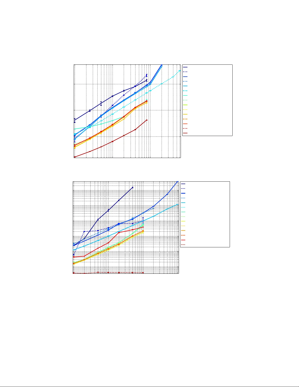
Non-sp arse Regulariza tion for Mul tiple Kernel Learning Non-Sparse Regularization for Multiple Kernel Learning Marius Kloft ∗ mkloft@cs.berkeley.edu University of California Computer Scienc e Division Berkeley, CA 94720-1758, USA Ulf Brefeld brefeld@y ahoo-inc.com Y aho o! R ese ar ch A vinguda Diagonal 177 08018 Bar c elona, Sp ain S¨ oren Sonnen burg ∗ soeren.sonnenburg@tuebingen.mpg.de F rie drich Miescher L ab or atory Max Planck So ciety Sp emannstr. 39, 72076 T¨ ubingen, Germany Alexander Zien zien@lifebiosystems.com LIFE Biosystems GmbH Poststr aße 34 69115 Heidelb er g, Germany Abstract Learning linear com binations of multiple k ernels is an app ealing strategy when the right c hoice of features is unkno wn. Previous approac hes to m ultiple k ernel learning (MKL) promote sparse kernel combinations to supp ort interpretabilit y and scalability . Unfortu- nately , this ` 1 -norm MKL is rarely observ ed to outp erform trivial baselines in practical applications. T o allow for robust k ernel mixtures, we generalize MKL to arbitrary norms. W e devise new insights on the connection betw een several existing MKL formulations and dev elop t w o eﬃcien t interle ave d optimization strategies for arbitrary norms, lik e ` p -norms with p > 1. Empirically , w e demonstrate that the in terlea v ed optimization strategies are m uch faster compared to the commonly used wrapp er approac hes. A theoretical analysis and an exp erimen t on controlled artiﬁcial data exp eriment sheds light on the appropriate- ness of sparse, non-sparse and ` ∞ -norm MKL in v arious scenarios. Empirical applications of ` p -norm MKL to three real-w orld problems from computational biology show that non- sparse MKL achiev es accuracies that go b eyond the state-of-the-art. Keyw ords: m ultiple kernel learning, learning kernels, non-sparse, support vector ma- c hine, conv ex conjugate, blo ck co ordinate descent, large scale optimization, bioinformatics, generalization bounds 1. In tro duction Kernels allow to decouple machine learning from data represen tations. Finding an appro- priate data represen tation via a kernel function immediately op ens the do or to a v ast w orld ∗ . Also at Mac hine Learning Group, T ec hnisc he Univ ersit¨ at Berlin, F ranklinstr. 28/29, FR 6-9, 10587 Berlin, Germany . 1 Kloft, Brefeld, Sonnenburg, and Zien of p ow erful mac hine learning mo dels (e.g. Sch¨ olk opf and Smola, 2002) with many eﬃcien t and reliable oﬀ-the-shelf implementations. This has prop elled the dissemination of machine learning tec hniques to a wide range of div erse application domains. Finding an appropriate data abstraction—or even engineering the b est kernel—for the problem at hand is not alwa ys trivial, though. Starting with cross-v alidation (Stone, 1974), whic h is probably the most prominent approach to general mo del selection, a great many approac hes to selecting the righ t kernel(s) hav e b een deplo y ed in the literature. Kernel target alignmen t (Cristianini et al., 2002; Cortes et al., 2010b) aims at learning the entries of a k ernel matrix by using the outer pro duct of the lab el vector as the ground- truth. Chap elle et al. (2002) and Bousquet and Herrmann (2002) minimize estimates of the generalization error of supp ort vector machines (SVMs) using a gradien t descent algorithm o v er the set of parameters. Ong et al. (2005) study h yp erk ernels on the space of k ernels and alternativ e approac hes include selecting kernels b y DC programming (Argyriou et al., 2008) and semi-inﬁnite programming ( ¨ Oz¨ og ¨ ur-Aky¨ uz and W eb er, 2008; Gehler and Now ozin, 2008). Although ﬁnding non-linear k ernel mixtures (G¨ onen and Alpaydin, 2008; V arma and Babu, 2009) generally results in non-con v ex optimization problems, Cortes et al. (2009b) sho w that conv ex relaxations ma y b e obtained for sp ecial cases. Ho w ev er, learning arbitrary k ernel com binations is a problem to o general to allow for a general optimal solution—b y fo cusing on a restricted scenario, it is p ossible to achiev e guaran teed optimality . In their seminal w ork, Lanckriet et al. (2004) consider training an SVM along with optimizing the linear com bination of several p ositiv e semi-deﬁnite matrices, K = P M m =1 θ m K m , sub ject to the trace constrain t tr( K ) ≤ c and requiring a v alid com bined k ernel K  0. This spawned the new ﬁeld of multiple kernel le arning (MKL), the automatic com bination of sev eral kernel functions. Lanc kriet et al. (2004) sho w that their sp eciﬁc v ersion of the MKL task can b e reduced to a conv ex optimization problem, namely a semi- deﬁnite programming (SDP) optimization problem. Though conv ex, how ev er, the SDP approac h is computationally to o expensive for practical applications. Th us muc h of the subsequen t researc h fo cuses on devising more eﬃcien t optimization pro cedures. One conceptual milestone for developing MKL into a tool of practical utility is simply to constrain the mixing co eﬃcients θ to be non-negativ e: by ob viating the complex con- strain t K  0, this small restriction allows one to transform the optimization problem in to a quadratically constrained program, hence drastically reducing the computational burden. While the original MKL ob jective is stated and optimized in dual space, alternativ e form u- lations ha v e b een studied. F or instance, Bach et al. (2004) found a corresp onding primal problem, and Rubinstein (2005) decomposed the MKL problem in to a min-max problem that can b e optimized b y mirror-pro x algorithms (Nemiro vski, 2004). The min-max formu- lation has b een indep endently prop osed by Sonnen burg et al. (2005). They use it to recast MKL training as a semi-inﬁnite linear program. Solving the latter with column generation (e.g., Nash and Sofer, 1996) amounts to rep eatedly training an SVM on a mixture kernel while iteratively reﬁning the mixture coeﬃcients θ . This immediately lends itself to a con- v enien t implemen tation b y a wrapp er approac h. These wrapp er algorithms directly b eneﬁt from eﬃcien t SVM optimization routines (cf., e.g., F an et al., 2005; Joac hims, 1999) and are no w commonly deploy ed in recen t MKL solvers (e.g., Rak otomamonjy et al., 2008; Xu et al., 2009), thereb y allowing for large-scale training (Sonnen burg et al., 2005, 2006a). How ever, the complete training of several SVMs can still b e prohibitive for large data sets. F or this 2 Non-sp arse Regulariza tion for Mul tiple Kernel Learning reason, Sonnenburg et al. (2005) also prop ose to interlea ve the SILP with the SVM training whic h reduces the training time drastically . Alternative optimization schemes include lev el- set metho ds (Xu et al., 2009) and second order approaches (Chap elle and Rakotomamonjy , 2008). Szafranski et al. (2010), Nath et al. (2009), and Bach (2009) study comp osite and hierarc hical kernel learning approac hes. Finally , Zien and Ong (2007) and Ji et al. (2009) pro vide extensions for m ulti-class and multi-label settings, respectively . T o day , there exist tw o ma jor families of m ultiple kernel learning models. The ﬁrst is c haracterized by Iv ano v regularization (Iv anov et al., 2002) o v er the mixing co eﬃcien ts (Rak otomamonjy et al., 2007; Zien and Ong, 2007). F or the Tikhono v-regularized optimiza- tion problem (Tikhono v and Arsenin, 1977), there is an additional parameter controlling the regularization of the mixing co eﬃcients (V arma and Ra y, 2007). All the ab ov e men tioned multiple kernel learning formulations promote sp arse solutions in terms of the mixing co eﬃcients. The desire for sparse mixtures originates in practical as well as theoretical reasons. First, sparse com binations are easier to in terpret. Second, irrelev ant (and p ossibly exp ensive) kernels functions do not need to b e ev aluated at testing time. Finally , sparseness app ears to b e handy also from a technical p oint of view, as the additional simplex constrain t k θ k 1 ≤ 1 simpliﬁes deriv ations and turns the problem in to a linearly constrained program. Nevertheless, sparseness is not alw a ys beneﬁcial in practice and sparse MKL is frequently observed to b e outp erformed b y a regular SVM using an un w eigh ted-sum k ernel K = P m K m (Cortes et al., 2008). Consequen tly , despite all the substantial progress in the ﬁeld of MKL, there still remains an unsatisﬁed need for an approac h that is really useful for practical applications: a mo del that has a go o d c hance of impro ving the accuracy (o v er a plain sum k ernel) together with an implemen tation that matches today’s standards (i.e., that can b e trained on 10,000s of data points in a reasonable time). In addition, since the ﬁeld has gro wn several comp eting MKL form ulations, it seems timely to consolidate the set of mo dels. In this article we argue that all of this is now achiev able. 1.1 Outline of the Presen ted Ac hiev ements On the theoretical side, w e cast multiple k ernel learning as a general regularized risk mini- mization problem for arbitrary con v ex loss functions, Hilb ertian regularizers, and arbitrary norm-p enalties on θ . W e ﬁrst sho w that the ab ov e men tioned Tikhonov and Iv anov regu- larized MKL v ariants are equiv alent in the sense that they yield the same set of hypotheses. Then w e deriv e a dual represen tation and show that a v ariety of metho ds are sp ecial cases of our ob jective. Our optimization problem subsumes state-of-the-art approac hes to multiple k ernel learning, co v ering sparse and non-sparse MKL b y arbitrary p -norm regularization (1 ≤ p ≤ ∞ ) on the mixing co eﬃcien ts as well as the incorp oration of prior knowledge b y allowing for non-isotropic regularizers. As w e demonstrate, the p -norm regularization includes both important sp ecial cases (sparse 1-norm and plain sum ∞ -norm) and oﬀers the potential to elev ate predictiv e accuracy ov er b oth of them. With regard to the implementation, we in tro duce an appealing and eﬃcien t optimization strategy whic h grounds on an exact up date in closed-form in the θ -step; hence rendering exp ensiv e semi-inﬁnite and ﬁrst- or second-order gradien t metho ds unnecessary . By uti- lizing pro ven working set optimization for SVMs, p -norm MKL can no w b e trained highly 3 Kloft, Brefeld, Sonnenburg, and Zien eﬃcien tly for all p ; in particular, w e outpace other curren t 1-norm MKL implemen tations. Moreo v er our implementation emplo ys k ernel caching tec hniques, whic h enables training on ten thousands of data p oin ts or thousands of k ernels resp ectively . In con trast, most comp eting MKL softw are require all kernel matrices to be stored completely in memory , whic h restricts these methods to small data sets with limited n um b ers of k ernels. Our im- plemen tation is freely a v ailable within the SHOGUN mac hine learning to olb ox a v ailable at http://www.shogun- toolbox.org/ . Our claims are bac k ed up by experiments on artiﬁcial data and on a couple of real w orld data sets representing div erse, relev an t and challenging problems from the application do- main bioinformatics. Experiments on artiﬁcial data enable us to in v estigate the relationship b et w een prop erties of the true solution and the optimal choice of k ernel mixture regular- ization. The real w orld problems include the prediction of the sub cellular lo calization of proteins, the (transcription) starts of genes, and the function of enzymes. The results demonstrate (i) that com bining k ernels is no w tractable on large data sets, (ii) that it can pro vide cutting edge classiﬁcation accuracy , and (iii) that depending on the task at hand, diﬀeren t k ernel mixture regularizations are required for ac hieving optimal p erformance. In App endix A we present a ﬁrst theoretical analysis of non-sparse MKL. W e in tro duce a no v el ` 1 -to- ` p con v ersion tec hnique and use it to derive generalization b ounds. Based on these, we p erform a case study to compare a particular sparse with a non-sparse scenario. A basic v ersion of this work app eared in NIPS 2009 (Kloft et al., 2009a). The presen t article additionally oﬀers a more general and complete deriv ation of the main optimization problem, exemplary applications thereof, a simple algorithm based on a closed-form solution, tec hnical details of the implemen tation, a theoretical analysis, and additional exp erimental results. Parts of App endix A are based on Kloft et al. (2010) the presen t analysis how ever extends the previous publication b y a nov el con v ersion technique, an illustrative case study , and an improv ed presentation. Since its initial publication in Kloft et al. (2008), Cortes et al. (2009a), and Kloft et al. (2009a), non-sparse MKL has b een subsequen tly applied, extended, and further analyzed b y sev eral researc hers: V arma and Babu (2009) derive a pro jected gradient-based optimization metho d for ` 2 -norm MKL. Y u et al. (2010) present a more general dual view of ` 2 -norm MKL and sho w adv antages of ` 2 -norm ov er an unw eighted-sum kernel SVM on six bioinfor- matics data sets. Cortes et al. (2010a) provide generalization b ounds for ` 1 - and ` p ≤ 2 -norm MKL. The analytical optimization metho d presented in this pap er was indepe nden tly and in parallel disco vered b y Xu et al. (2010) and has also been studied in Roth and Fisc her (2007) and Ying et al. (2009) for ` 1 -norm MKL, and in Szafranski et al. (2010) and Nath et al. (2009) for composite kernel learning on small and medium scales. The remainder is structured as follo ws. W e deriv e non-sparse MKL in Section 2 and discuss relations to existing approac hes in Section 3. Section 4 introduces the no v el opti- mization strategy and its implementation. W e report on our empirical results in Section 5. Section 6 concludes. 2. Multiple Kernel Learning – A Regularization View In this section we cast multiple k ernel learning in to a uniﬁed framework: we present a regularized loss minimization formulation with additional norm constrain ts on the k ernel 4 Non-sp arse Regulariza tion for Mul tiple Kernel Learning mixing co eﬃcien ts. W e show that it comprises many p opular MKL v arian ts currently discussed in the literature, including seemingly diﬀeren t ones. W e derive generalized dual optimization problems without making sp eciﬁc assumptions on the norm regularizers or the loss function, b eside that the latter is conv ex. Our formu- lation co v ers binary classiﬁcation and regression tasks and can easily b e extended to multi- class classiﬁcation and structural learning se ttings using appropriate conv ex loss functions and join t k ernel extensions. Prior kno wledge on k ernel mixtures and k ernel asymmetries can be incorp orated b y non-isotropic norm regularizers. 2.1 Preliminaries W e begin with reviewing the classical sup ervised learning setup. Giv en a labeled sample D = { ( x i , y i ) } i =1 ...,n , where the x i lie in some input space X and y i ∈ Y ⊂ R , the goal is to ﬁnd a hypothesis h ∈ H , that generalizes well on new and unseen data. Regularized risk minimization returns a minimizer h ∗ , h ∗ ∈ argmin h R emp ( h ) + λ Ω( h ) , where R emp ( h ) = 1 n P n i =1 V ( h ( x i ) , y i ) is the empirical risk of hypothesis h w.r.t. a con v ex loss function V : R × Y → R , Ω : H → R is a regularizer, and λ > 0 is a trade-oﬀ parameter. W e consider linear mo dels of the form h ˜ w ,b ( x ) = h ˜ w , ψ ( x ) i + b, (1) together with a (p ossibly non-linear) mapping ψ : X → H to a Hilb ert space H (e.g., Sc h¨ olkopf et al., 1998; M ¨ uller et al., 2001) and constrain the regularization to b e of the form Ω( h ) = 1 2 k ˜ w k 2 2 whic h allows to kernelize the resulting mo dels and algorithms. W e will later make use of k ernel functions k ( x , x 0 ) = h ψ ( x ) , ψ ( x 0 ) i H to compute inner pro ducts in H . 2.2 Regularized Risk Minimization with Multiple Kernels When learning with m ultiple k ernels, w e are giv en M diﬀeren t feature mappings ψ m : X → H m , m = 1 , . . . M , eac h giving rise to a repro ducing k ernel k m of H m . Con vex approaches to m ultiple k ernel learning consider linear k ernel mixtures k θ = P θ m k m , θ m ≥ 0. Compared to Eq. (1), the primal mo del for learning with m ultiple k ernels is extended to h ˜ w ,b, θ ( x ) = M X m =1 p θ m h ˜ w m , ψ m ( x ) i H m + b = h ˜ w , ψ θ ( x ) i H + b (2) where the parameter v ector ˜ w and the comp osite feature map ψ θ ha v e a blo ck structure ˜ w = ( ˜ w > 1 , . . . , ˜ w > M ) > and ψ θ = √ θ 1 ψ 1 × . . . × √ θ M ψ M , respectively . In learning with multiple kernels we aim at minimizing the loss on the training data w.r.t. the optimal kernel mixture P M m =1 θ m k m in addition to regularizing θ to a v oid ov erﬁtting. Hence, in terms of regularized risk minimization, the optimization problem becomes inf ˜ w ,b, θ : θ ≥ 0 1 n n X i =1 V M X m =1 p θ m h ˜ w m , ψ m ( x i ) i H m + b, y i ! + λ 2 M X m =1 k ˜ w m k 2 H m + ˜ µ ˜ Ω[ θ ] , (3) 5 Kloft, Brefeld, Sonnenburg, and Zien for ˜ µ > 0. Note that the ob jective v alue of Eq. (3) is an upp er b ound on the training error. Previous approaches to m ultiple k ernel learning employ regularizers of the form ˜ Ω( θ ) = k θ k 1 to promote sparse kernel mixtures. By contrast, w e propose to use con v ex regularizers of the form ˜ Ω( θ ) = k θ k 2 , where k · k 2 is an arbitrary norm in R M , p ossibly allo wing for non- sparse solutions and the incorp oration of prior kno wledge. The non-conv exit y arising from the √ θ m ˜ w m pro duct in the loss term of Eq. (3) is not inherent and can b e resolv ed by substituting w m ← √ θ m ˜ w m . F urthermore, the regularization parameter and the sample size can b e decoupled by introducing ˜ C = 1 nλ (and adjusting µ ← ˜ µ λ ) whic h has fa v orable scaling prop erties in practice. W e obtain the following conv ex optimization problem (Boyd and V anden b erghe, 2004) that has also been considered b y (V arma and Ra y, 2007) for hinge loss and an ` 1 -norm regularizer inf w ,b, θ : θ ≥ 0 ˜ C n X i =1 V M X m =1 h w m , ψ m ( x i ) i H m + b, y i ! + 1 2 M X m =1 k w m k 2 H m θ m + µ k θ k 2 , (4) where w e use the con ven tion that t 0 = 0 if t = 0 and ∞ otherwise. An alternativ e approac h has b een studied b y Rak otomamonjy et al. (2007) and Zien and Ong (2007), again using hinge loss and ` 1 -norm. They upp er bound the v alue of the regularizer k θ k 1 ≤ 1 and incorp orate the latter as an additional constrain t into the optimization problem. F or C > 0, they arrive at the following problem which is the primary ob ject of in v estigation in this paper. Primal MKL Optimization Problem inf w ,b, θ : θ ≥ 0 C n X i =1 V  M X m =1 h w m , ψ m ( x i ) i H m + b, y i  + 1 2 M X m =1 k w m k 2 H m θ m (P) s.t. k θ k 2 ≤ 1 . It is imp ortant to note here that, while the Iv ano v regularization in (4) has two regu- larization parameters ( C and µ ), the ab ov e Tikhonov regularization (P) has only one ( C only). Our ﬁrst contribution shows that, despite the additional regularization parameter, b oth MKL v ariants are equiv alen t, in the sense that tra v ersing the regularization paths yields the same binary classiﬁcation functions. Theorem 1. L et k · k b e a norm on R M , b e V a c onvex loss function. Supp ose for the optimal w ∗ in Optimization Pr oblem (P) it holds w ∗ 6 = 0 . Then, for e ach p air ( ˜ C , µ ) ther e exists C > 0 such that for e ach optimal solution ( w , b, θ ) of Eq. (4) using ( ˜ C , µ ) , we have that ( w , b, κ θ ) is also an optimal solution of Optimization Pr oblem (P) using C , and vic e versa, wher e κ > 0 is a multiplic ative c onstant. F or the pro of we need Prop. 11, whic h justiﬁes switc hing from Iv ano v to Tikhono v regularization, and back, if the regularizer is tigh t. W e refer to App endix B for the prop osition and its pro of. 6 Non-sp arse Regulariza tion for Mul tiple Kernel Learning Pr o of. of Theorem 1 Let b e ( ˜ C , µ ) > 0. In order to apply Prop. 11 to (4), w e sho w that condition (37) in Prop. 11 is satisﬁed, i.e., that the regularizer is tight. Supp ose on the con trary , that Optimization Problem (P) yields the same inﬁmum re- gardless of whether w e require k θ k 2 ≤ 1 , (5) or not. Then this implies that in the optimal p oin t we hav e P M m =1 k w ∗ m k 2 2 θ ∗ m = 0, hence, k w ∗ m k 2 2 θ ∗ m = 0 , ∀ m = 1 , . . . , M . (6) Since all norms on R M are equiv alent (e.g., Rudin, 1991), there exists a L < ∞ such that k θ ∗ k ∞ ≤ L k θ ∗ k . In particular, we ha ve k θ ∗ k ∞ < ∞ , from which we conclude b y (6), that w m = 0 holds for all m , which contradicts our assumption. Hence, Prop. 11 can be applied, 1 whic h yields that (4) is equiv alent to inf w ,b, θ ˜ C n X i =1 V  M X m =1 h w m , ψ m ( x ) i + b, y i  + 1 2 M X m =1 k w m k 2 2 θ m s.t. k θ k 2 ≤ τ , for some τ > 0. Consider the optimal solution ( w ? , b ? , θ ? ) corresp onding to a giv en parametrization ( ˜ C , τ ). F or an y λ > 0, the bijective transformation ( ˜ C , τ ) 7→ ( λ − 1 / 2 ˜ C , λτ ) will yield ( w ? , b ? , λ 1 / 2 θ ? ) as optimal solution. Applying the transformation with λ := 1 /τ and setting C = ˜ C τ 1 2 as w ell as κ = τ − 1 / 2 yields Optimization Problem (P), whic h w as to b e sho wn. Zien and Ong (2007) also show that the MKL optimization problems by Bach et al. (2004), Sonnen burg et al. (2006a), and their own formulation are equiv alent. As a main implication of Theorem 1 and by using the result of Zien and Ong it follows that the optimization problem of V arma and Ray (V arma and Ra y, 2007) lies in the same equiv alence class as (Bach et al., 2004; Sonnen burg et al., 2006a; Rakotomamonjy et al., 2007; Zien and Ong, 2007). In addition, our result shows the coupling b etw een trade-oﬀ parameter C and the regularization parameter µ in Eq. (4): tw eaking one also changes the other and vice v ersa. Theorem 1 implies that optimizing C in Optimization Problem (P) implicitly searc hes the regularization path for the parameter µ of Eq. (4). In the remainder, we will therefore fo cus on the formulation in Optimization Problem (P), as a single parameter is preferable in terms of model selection. 2.3 MKL in Dual Space In this section we study the generalized MKL approac h of the previous section in the dual space. Let us b egin with rewriting Optimization Problem (P) by expanding the decision 1. Note that after a coordinate transformation, we can assume that H is ﬁnite dimensional (see Sch¨ olk opf et al., 1999). 7 Kloft, Brefeld, Sonnenburg, and Zien v alues in to slack v ariables as follo ws inf w ,b, t , θ : θ ≥ 0 C n X i =1 V ( t i , y i ) + 1 2 M X m =1 k w m k 2 H m θ m (7) s.t. ∀ i : M X m =1 h w m , ψ m ( x i ) i H m + b = t i ; k θ k 2 ≤ 1 , where k · k is an arbitrary norm in R m and k · k H M denotes the Hilb ertian norm of H m . Ap- plying Lagrange’s theorem re-incorp orates the constrain ts into the ob jectiv e by in tro ducing Lagrangian multipliers α ∈ R n and β ∈ R + . 2 The Lagrangian saddle p oint problem is then giv en by sup α ,β : β ≥ 0 inf w ,b, t , θ ≥ 0 C n X i =1 V ( t i , y i ) + 1 2 M X m =1 k w m k 2 H m θ m (8) − n X i =1 α i M X m =1 h w m , ψ m ( x i ) i H m + b − t i ! + β  1 2 k θ k 2 − 1 2  . Denoting the Lagrangian by L and setting its ﬁrst partial deriv ativ es with resp ect to w and b to 0 rev eals the optimality conditions 1 > α = 0; (9a) w m = θ m n X i =1 α i ψ m ( x i ) , ∀ m = 1 , . . . , M . (9b) Resubstituting the ab ov e equations yields sup α : 1 > α =0 , β : β ≥ 0 inf t , θ ≥ 0 C n X i =1 ( V ( t i , y i ) + α i t i ) − 1 2 M X m =1 θ m α > K m α + β  1 2 k θ k 2 − 1 2  , whic h can also b e written in terms of unconstrained θ , b ecause the supremum with resp ect to θ is attained for non-negative θ ≥ 0. W e arriv e at sup α : 1 > α =0 , β ≥ 0 − C n X i =1 sup t i  − α i C t i − V ( t i , y i )  − β sup θ 1 2 β M X m =1 θ m α > K m α − 1 2 k θ k 2 ! − 1 2 β . As a consequence, w e no w may express the Lagrangian as 3 sup α : 1 > α =0 , β ≥ 0 − C n X i =1 V ∗  − α i C , y i  − 1 2 β     1 2  α > K m α  M m =1     2 ∗ − 1 2 β , (10) where h ∗ ( x ) = sup u x > u − h ( u ) denotes the F enchel-Legendre conjugate of a function h and k · k ∗ denotes the dual norm , i.e., the norm deﬁned via the identit y 1 2 k · k 2 ∗ :=  1 2 k · k 2  ∗ . 2. Note that, in contrast to the standard SVM dual deriviations, here α is a v ariable that ranges ov er all of R n , as it is incorp orates an equality constraint. 3. W e employ the notation s = ( s 1 , . . . , s M ) > = ( s m ) M m =1 for s ∈ R M . 8 Non-sp arse Regulariza tion for Mul tiple Kernel Learning In the follo wing, we call V ∗ the dual loss . Eq. (10) now has to b e maximized with resp ect to the dual v ariables α , β , sub ject to 1 > α = 0 and β ≥ 0. Let us ignore for a momen t the non-negativit y constraint on β and solve ∂ L /∂ β = 0 for the unbounded β . Setting the partial deriv ativ e to zero allo ws to express the optimal β as β =     1 2  α > K m α  M m =1     ∗ . (11) Ob viously , at optimality , we alwa ys hav e β ≥ 0. W e thus discard the corresp onding constrain t from the optimization problem and plugging Eq. (11) in to Eq. (10) results in the follo wing dual optimization problem whic h now solely dep ends on α : Dual MKL Optimization Problem sup α : 1 > α =0 − C n X i =1 V ∗  − α i C , y i  − 1 2      α > K m α  M m =1     ∗ . (D) The ab o v e dual generalizes multiple k ernel learning to arbitrary conv ex loss functions and norms. 4 Note that if the loss function is con tin uous (e.g., hinge loss), the supremum is also a maximum. The threshold b can b e recov ered from the solution by applying the KKT conditions. The ab ov e dual can b e characterized as follows. W e start by noting that the expression in Optimization Problem (D) is a comp osition of tw o terms, ﬁrst, the left hand side term, whic h dep ends on the conjugate loss function V ∗ , and, second, the righ t hand side term which dep ends on the conjugate norm. The righ t hand side can b e in terpreted as a regularizer on the quadratic terms that, according to the c hosen norm, smo othens the solutions. Hence w e hav e a decomp osition of the dual into a loss term (in terms of the dual loss) and a regularizer (in terms of the dual norm). F or a speciﬁc c hoice of a pair ( V , k · k ) we can immediately recov er the corresp onding dual b y computing the pair of conjugates ( V ∗ , k · k ∗ ) (for a comprehensiv e list of dual losses see Rifkin and Lipp ert, 2007, T able 3). In the next section, this is illustrated b y means of w ell-known loss functions and regularizers. A t this p oin t we w ould like to highligh t some properties of Optimization Problem (D) that arise due to our dualization tec hnique. While approaches that ﬁrstly apply the rep- resen ter theorem and secondly optimize in the primal suc h as Chap elle (2006) also can emplo y general loss functions, the resulting loss terms dep end on all optimization v ariables. By con trast, in our formulation the dual loss terms are of a muc h simpler structure and they only dep end on a single optimization v ariable α i . A similar dualization technique yielding singly-v alued dual loss terms is presen ted in Rifkin and Lipp ert (2007); it is based on F enchel dualit y and limited to strictly positive deﬁnite k ernel matrices. Our tec hnique, whic h uses Lagrangian dualit y , extends the latter by allo wing for p ositiv e semi-deﬁnite k ernel matrices. 4. W e can even employ non-conv ex losses and still the dual will be a con v ex problem; ho w ev er, it might suﬀer from a duality gap. 9 Kloft, Brefeld, Sonnenburg, and Zien 3. Instantiations of the Mo del In this section w e show that existing MKL-based learners are subsumed b y the generalized form ulation in Optimization Problem (D). 3.1 Supp ort V ector Mac hines with Un w eighted-Sum Kernels First w e note that the support v ector mac hine with an un weigh ted-sum k ernel can b e recov- ered as a special case of our mo del. T o see this, w e consider the regularized risk minimization problem using the hinge loss function V ( t, y ) = max(0 , 1 − ty ) and the regularizer k θ k ∞ . W e then can obtain the corresponding dual in terms of F enchel-Legendre conjugate functions as follo ws. W e ﬁrst note that the dual loss of the hinge loss is V ∗ ( t, y ) = t y if − 1 ≤ t y ≤ 0 and ∞ elsewise (Rifkin and Lipp ert, 2007, T able 3). Hence, for each i the term V ∗  − α i C , y i  of the generalized dual, i.e., Optimization Problem (D), translates to − α i C y i , provided that 0 ≤ α i y i ≤ C . Emplo ying a v ariable substitution of the form α new i = α i y i , Optimization Problem (D) translates to max α 1 > α − 1 2      α > Y K m Y α  M m =1     ∗ , s.t. y > α = 0 and 0 ≤ α ≤ C 1 , (12) where we denote Y = diag ( y ). The primal ` ∞ -norm p enalty k θ k ∞ is dual to k θ k 1 , hence, via the identit y k · k ∗ = k · k 1 the righ t hand side of the last equation translates to P M m =1 α > Y K m Y α . Combined with (12) this leads to the dual sup α 1 > α − 1 2 M X m =1 α > Y K m Y α , s.t. y > α = 0 and 0 ≤ α ≤ C 1 , whic h is precisely an SVM with an un w eigh ted-sum kernel. 3.2 QCQP MKL of Lanc kriet et al. (2004) A common approach in m ultiple k ernel learning is to employ regularizers of the form Ω( θ ) = k θ k 1 . (13) This so-called ` 1 -norm regularizers are speciﬁc instances of sp arsity-inducing regularizers. The obtained kernel mixtures usually hav e a considerably large fraction of zero en tries, and hence equip the MKL problem b y the fa v or of interpretable solutions. Sparse MKL is a sp ecial case of our framew ork; to see this, note that the conjugate of (13) is k · k ∞ . Recalling the deﬁnition of an ` p -norm, the righ t hand side of Optimization Problem (D) translates to max m ∈{ 1 ,...,M } α > Y K m Y α . The maximum can subsequen tly b e expanded into a slac k v ariable ξ , resulting in sup α , ξ 1 > α − ξ s.t. ∀ m : 1 2 α > Y K m Y α ≤ ξ ; y > α = 0 ; 0 ≤ α ≤ C 1 , whic h is the original QCQP formulation of MKL, ﬁrstly given by Lanckriet et al. (2004). 10 Non-sp arse Regulariza tion for Mul tiple Kernel Learning 3.3 ` p -Norm MKL Our MKL formulation also allows for robust kernel mixtures b y employing an ` p -norm constrain t with p > 1, rather than an ` 1 -norm constrain t, on the mixing coeﬃcients (Kloft et al., 2009a). The follo wing identit y holds  1 2 k · k 2 p  ∗ = 1 2 k · k 2 p ∗ , where p ∗ := p p − 1 is the conjugated exp onen t of p , and w e obtain for the dual norm of the ` p -norm: k · k ∗ = k · k p ∗ . This leads to the dual problem sup α : 1 > α = 0 − C n X i =1 V ∗  − α i C , y i  − 1 2      α > K m α  M m =1     p ∗ . In the sp ecial case of hinge loss minimization, we obtain the optimization problem sup α 1 > α − 1 2      α > Y K m Y α  M m =1     p ∗ , s.t. y > α = 0 and 0 ≤ α ≤ C 1 . 3.4 A Smo oth V arian t of Group Lasso Y uan and Lin (2006) studied the following optimization problem for the sp ecial case H m = R d m and ψ m = id R d m , also known as group lasso, min w C 2 n X i =1 y i − M X m =1 h w m , ψ m ( x i ) i H m ! 2 + 1 2 M X m =1 k w m k H m . (14) The ab ov e problem has been solved by activ e set metho ds in the primal (Roth and Fischer, 2008). W e sk etc h an alternativ e approach based on dual optimization. First, w e note that Eq. (14) can b e equiv alen tly expressed as (Micc helli and Pon til, 2005, Lemma 26) inf w , θ : θ ≥ 0 C 2 n X i =1 y i − M X m =1 h w m , ψ m ( x i ) i H m ! 2 + 1 2 M X m =1 k w m k 2 H m θ m , s.t. k θ k 2 1 ≤ 1 . The dual of V ( t, y ) = 1 2 ( y − t ) 2 is V ∗ ( t, y ) = 1 2 t 2 + ty and th us the corresp onding group lasso dual can b e written as max α y > α − 1 2 C k α k 2 2 − 1 2      α > Y K m Y α  M m =1     ∞ , (15) whic h can b e expanded in to the follo wing QCQP sup α ,ξ y > α − 1 2 C k α k 2 2 − ξ (16) s.t. ∀ m : 1 2 α > Y K m Y α ≤ ξ . 11 Kloft, Brefeld, Sonnenburg, and Zien F or small n , the latter formulation can b e handled eﬃcien tly by QCQP solvers. Ho w ev er, the quadratic constrain ts caused by the non-smo oth ` ∞ -norm in the ob jective still are computationally to o demanding. As a remedy , we prop ose the following unconstrained v ariant based on ` p -norms (1 < p < ∞ ), giv en b y max α y > α − 1 2 C k α k 2 2 − 1 2      α > Y K m Y α  M m =1     p ∗ . It is straigh t forward to verify that the ab o v e ob jective function is diﬀeren tiable in an y α ∈ R n (in particular, notice that the ` p -norm function is diﬀerentiable for 1 < p < ∞ ) and hence the ab ov e optimization problem can b e solv ed very eﬃciently b y , for example, limited memory quasi-Newton descen t methods (Liu and No cedal, 1989). 3.5 Densit y Lev el-Set Estimation Densit y level-set estimators are frequently used for anomaly/nov elty detection tasks (Mark ou and Singh, 2003a,b). Kernel approaches, suc h as one-class SVMs (Sch¨ olk opf et al., 2001) and Support V ector Domain Descriptions (T ax and Duin, 1999) can b e cast in to our MKL framework b y emplo ying loss functions of the form V ( t ) = max(0 , 1 − t ). This gives rise to the primal inf w , θ : θ ≥ 0 C n X i =1 max 0 , M X m =1 h w m , ψ m ( x i ) i H m ! + 1 2 M X m =1 k w m k 2 H m θ m , s.t. k θ k 2 ≤ 1 . Noting that the dual loss is V ∗ ( t ) = t if − 1 ≤ t ≤ 0 and ∞ elsewise, we obtain the following generalized dual sup α 1 > α − 1 2      α > K m α  M m =1     p ∗ , s.t. 0 ≤ α ≤ C 1 , whic h has b een studied b y Sonnen burg et al. (2006a) and Rak otomamonjy et al. (2008) for ` 1 -norm, and by Kloft et al. (2009b) for ` p -norms. 3.6 Non-Isotropic Norms In practice, it is often desirable for an exp ert to incorp orate prior kno wledge ab out the problem domain. F or instance, an exp ert could provide estimates of the in teractions of k ernels { K 1 , ..., K M } in the form of an M × M matrix E . Alternatively , E could be obtained b y computing pairwise k ernel alignments E ij = k K i k k K j k giv en a dot pro duct on the space of k ernels suc h as the F rob enius dot pro duct (Ong et al., 2005). In a third scenario, E could b e a diagonal matrix encoding the a priori imp ortance of k ernels—it might b e kno wn from pilot studies that a subset of the emplo y ed kernels is inferior to the remaining ones. All those scenarios can b e easily handled within our framew ork by considering non- isotropic regularizers of the form 5 k θ k E − 1 = p θ > E − 1 θ with E  0 , 5. This idea is inspired by the Mahalanobis distance (Mahalanobis, 1936). 12 Non-sp arse Regulariza tion for Mul tiple Kernel Learning where E − 1 is the matrix inv erse of E . The dual norm is again deﬁned via 1 2 k · k 2 ∗ :=  1 2 k · k 2 E − 1  ∗ and the following easily-to-verify identit y ,  1 2 k · k 2 E − 1  ∗ = 1 2 k · k 2 E , leads to the dual, sup α : 1 > α = 0 − C n X i =1 V ∗  − α i C , y i  − 1 2      α > K m α  M m =1     E , whic h is the desired non-isotropic MKL problem. 4. Optimization Strategies The dual as given in Optimization Problem (D) does not lend itself to eﬃcient large-scale optimization in a straigh t-forw ard fashion, for instance by direct application of standard approac hes lik e gradient descen t. Instead, it is b eneﬁcial to exploit the structure of the MKL cost function b y alternating b et w een optimizing w.r.t. the mixings θ and w.r.t. the remaining v ariables. Most recent MKL solvers (e.g., Rak otomamonjy et al., 2008; Xu et al., 2009; Nath et al., 2009) do so by setting up a t wo-la y er optimization pro cedure: a master problem, which is parameterized only b y θ , is solved to determine the k ernel mixture; to solv e this master problem, rep eatedly a sla ve problem is solved whic h amounts to train- ing a standard SVM on a mixture k ernel. Importantly , for the slav e problem, the mixture co eﬃcien ts are ﬁxed, suc h that con ven tional, eﬃcien t SVM optimizers can b e recycled. Con- sequen tly these tw o-la yer procedures are commonly implemented as wr app er approaches. Alb eit app earing adv an tageous, wrapp er metho ds suﬀer from tw o shortcomings: (i) Due to k ernel cac he limitations, the kernel matrices ha v e to b e pre-computed and stored or many k ernel computations ha ve to b e carried out repeatedly , inducing hea vy wastage of either memory or time. (ii) The slav e problem is alwa ys optimized to the end (and man y con- v ergence proofs seem to require this), although most of the computational time is sp end on the non-optimal mixtures. Certainly sub optimal sla v e solutions would already suﬃce to impro v e far-from-optimal θ in the master problem. Due to these problems, MKL is prohibitive when learning with a multitude of kernels and on large-scale data sets as commonly encoun tered in many data-intense real world applications suc h as bioinformatics, w eb mining, databases, and computer securit y . The optimization approach presen ted in this pap er decomp oses the MKL problem in to smaller subproblems (Platt, 1999; Joac hims, 1999; F an et al., 2005) b y establishing a wrapp er-lik e sc heme within the decomp osition algorithm. Our algorithm is embedded into the large-scale framework of Sonnen burg et al. (2006a) and extends it to the optimization of non-sparse kernel mixtures induced b y an ` p -norm p enalt y . Our strategy alternates b et w een minimizing the primal problem (7) w.r.t. θ via a simple analytical update form ula and with incomplete optimization w.r.t. all other v ariables whic h, how ever, is performed in terms of the dual v ariables α . Optimization w.r.t. α is p erformed b y ch unking optimizations with minor iterations. Conv ergence of our algorithm is pro ven under typical technical regularit y assumptions. 13 Kloft, Brefeld, Sonnenburg, and Zien 4.1 A Simple W rapp er Approac h Based on an Analytical Up date W e ﬁrst presen t an easy-to-implemen t wrapp er version of our optimization approac h to m ultiple k ernel learning. The in terlea v ed decomp osition algorithm is deferred to the next section. T o derive the new algorithm, we ﬁrst revisit the primal problem, i.e. inf w ,b, θ : θ ≥ 0 C n X i =1 V M X m =1 h w m , ψ m ( x i ) i H m + b, y i ! + 1 2 M X m =1 k w m k 2 H m θ m , s.t. k θ k 2 ≤ 1 . ( P ) In order to obtain an eﬃcien t optimization strategy , w e divide the v ariables in the abov e OP into t w o groups, ( w , b ) on one hand and θ on the other. In the follo wing w e will deriv e an algorithm whic h alternatingly op erates on those t wo groups via a block coordinate descen t algorithm, also kno wn as the non-line ar blo ck Gauss-Seidel metho d . Thereby the optimization w.r.t. θ will be carried out analytically and the ( w , b )-step will be computed in the dual, if needed. The basic idea of our ﬁrst approac h is that for a giv en, ﬁxed set of primal v ariables ( w , b ), the optimal θ in the primal problem (P) can b e calculated analytically . In the subsequent deriv ations w e employ non-sparse norms of the form k θ k p = ( P M m =1 θ p m ) 1 /p , 1 < p < ∞ . 6 The follo wing prop osition giv es an analytic up date form ula for θ giv en ﬁxed remaining v ariables ( w , b ) and will b ecome the core of our prop osed algorithm. Prop osition 2. L et V b e a c onvex loss function, b e p > 1 . Given ﬁxe d (p ossibly sub optimal) w 6 = 0 and b , the minimal θ in Optimization Pr oblem (P) is attaine d for θ m = k w m k 2 p +1 H m  P M m 0 =1 k w m 0 k 2 p p +1 H m 0  1 /p , ∀ m = 1 , . . . , M . (17) Pr o of. 7 W e start the deriv ation, by equiv alently translating Optimization Problem (P) via Theorem 1 into inf w ,b, θ : θ ≥ 0 ˜ C n X i =1 V M X m =1 h w m , ψ m ( x i ) i H m + b, y i ! + 1 2 M X m =1 k w m k 2 H m θ m + µ 2 k θ k 2 p , (18) with µ > 0. Supp ose w e are giv en ﬁxed ( w , b ), then setting the partial deriv ativ es of the ab o v e ob jective w.r.t. θ to zero yields the following condition on the optimality of θ , − k w m k 2 H m 2 θ 2 m + µ · ∂  1 2 k θ k 2 p  ∂ θ m = 0 , ∀ m = 1 , . . . , M . (19) The ﬁrst deriv ativ e of the ` p -norm with resp ect to the mixing coeﬃcients can b e expressed as ∂  1 2 k θ k 2 p  ∂ θ m = θ p − 1 m k θ k 2 − p p , 6. While the reasoning also holds for weigh ted ` p -norms, the extension to more general norms, suc h as the ones describ ed in Section 3.6, is left for future work. 7. W e remark that a more general result can b e obtained b y an alternative pro of using H¨ older’s inequality (see Lemma 26 in Micchelli and Pon til, 2005). 14 Non-sp arse Regulariza tion for Mul tiple Kernel Learning and hence Eq. (19) translates into the follo wing optimalit y condition, ∃ ζ ∀ m = 1 , . . . , M : θ m = ζ k w m k 2 p +1 H m . (20) Because w 6 = 0, using the same argumen t as in the pro of of Theorem 1, the constrain t k θ k 2 p ≤ 1 in (18) is at the upp er b ound, i.e. k θ k p = 1 holds for an optimal θ . Inserting (20) in the latter equation leads to ζ =  P M m =1 k w m k 2 p/p +1 H m  1 /p . Resubstitution in to (20) yields the claimed formula (17). Second, we consider ho w to optimize Optimization Problem (P) w.r.t. the remaining v ariables ( w , b ) for a given set of mixing coeﬃcients θ . Since optimization often is consid- erably easier in the dual space, we ﬁx θ and build the partial Lagrangian of Optimization Problem (P) w.r.t. all other primal v ariables w , b . The resulting dual problem is of the form (detailed deriv ations omitted) sup α : 1 > α =0 − C n X i =1 V ∗  − α i C , y i  − 1 2 M X m =1 θ m α > K m α , (21) and the KKT conditions yield w m = θ m P n i =1 α i ψ m ( x i ) in the optimal point, hence k w m k 2 = θ 2 m α K m α , ∀ m = 1 , . . . , M . (22) W e now hav e all ingredients (i.e., Eqs. (17), (21)–(22)) to form ulate a simple macro-wrapper algorithm for ` p -norm MKL training: Algorithm 1 Simple ` p> 1 -norm MKL wr app er-b ase d tr aining algorithm. The analytic al up dates of θ and the SVM c omputations ar e optimize d alternatingly. 1: input: feasible α and θ 2: while optimality conditions are not satisﬁed do 3: Compute α according to Eq. (21) (e.g. SVM) 4: Compute k w m k 2 for all m = 1 , ..., M according to Eq. (22) 5: Update θ according to Eq. (17) 6: end while The ab ov e algorithm alternatingly solves a conv ex risk minimization machine (e.g. SVM) w.r.t. the actual mixture θ (Eq. (21)) and subsequen tly computes the analytical up date according to Eq. (17) and (22). It can, for example, be stopp ed based on c hanges of the ob jectiv e function or the duality gap within subsequen t iterations. 4.2 T o w ards Large-Scale MKL—Interlea ving SVM and MKL Optimization Ho w ev er, a disadv antage of the ab ov e wrapp er approac h still is that it deplo ys a full blo wn k ernel matrix. W e thus prop ose to in terleav e the SVM optimization of SVMligh t with the θ - and α -steps at training time. W e ha v e implemented this so-called interle ave d algorithm in Shogun for hinge loss, thereby promoting sparse solutions in α . This allo ws us to solely op erate on a small num ber of active v ariables. 8 The resulting in terlea v ed optimization 8. In practice, it turns out that the kernel matrix of active v ariables t ypically is ab out of the size 40 × 40, ev en when we deal with ten-thousands of examples. 15 Kloft, Brefeld, Sonnenburg, and Zien metho d is shown in Algorithm 2. Lines 3-5 are standard in c h unking based SVM solv ers and carried out by SVM light (note that Q is c hosen as describ ed in Joachims (1999)). Lines 6-7 compute SVM-ob jectiv e v alues. Finally , the analytical θ -step is carried out in Line 9. The algorithm terminates if the maximal KKT violation (c.f. Joachims, 1999) falls b elow a predetermined precision ε and if the normalized maximal constrain t violation | 1 − ω ω o ld | < ε mkl for the MKL-step, where ω denotes the MKL ob jectiv e function v alue (Line 8). Algorithm 2 ` p -Norm MKL chunking-b ase d tr aining algorithm via analytic al up date. Ker- nel weighting θ and (signe d) SVM α ar e optimize d interle avingly. The ac cur acy p ar ameter ε and the subpr oblem size Q ar e assume d to b e given to the algorithm. 1: Initialize: g m,i = ˆ g i = α i = 0, ∀ i = 1 , ..., n ; L = S = −∞ ; θ m = p p 1 / M , ∀ m = 1 , ..., M 2: iterate 3: Select Q v ariables α i 1 , . . . , α i Q based on the gradient ˆ g of (21) w.r.t. α 4: Store α old = α and then up date α according to (21) with respect to the selected v ariables 5: Up date gradient g m,i ← g m,i + P Q q =1 ( α i q − α old i q ) k m ( x i q , x i ), ∀ m = 1 , . . . , M , i = 1 , . . . , n 6: Compute the quadratic terms S m = 1 2 P i g m,i α i , q m = 2 θ 2 m S m , ∀ m = 1 , . . . , M 7: L o ld = L , L = P i y i α i , S o ld = S , S = P m θ m S m 8: if | 1 − L − S L o ld − S o ld | ≥ ε 9: θ m = ( q m ) 1 / ( p +1) /  P M m 0 =1 ( q m 0 ) p/ ( p +1)  1 /p , ∀ m = 1 , . . . , M 10: else 11: break 12: end if 13: ˆ g i = P m θ m g m,i for all i = 1 , . . . , n 4.3 Con v ergence Proof for p > 1 In the following, w e exploit the primal view of the ab ov e algorithm as a nonlinear block Gauss-Seidel metho d, to prov e con v ergence of our algorithms. W e ﬁrst need the following useful result ab out con v ergence of the nonlinear block Gauss-Seidel metho d in general. Prop osition 3 (Bertsek as, 1999, Prop. 2.7.1) . L et X = N M m =1 X m b e the Cartesian pr o duct of close d c onvex sets X m ⊂ R d m , b e f : X → R a c ontinuously diﬀer entiable function. Deﬁne the nonline ar blo ck Gauss-Seidel metho d r e cursively by letting x 0 ∈ X b e any fe asible p oint, and b e x k +1 m = argmin ξ ∈X m f  x k +1 1 , · · · , x k +1 m − 1 , ξ , x k m +1 , · · · , x k M  , ∀ m = 1 , . . . , M . (23) Supp ose that for e ach m and x ∈ X , the minimum min ξ ∈X m f ( x 1 , · · · , x m − 1 , ξ , x m +1 , · · · , x M ) (24) is uniquely attaine d. Then every limit p oint of the se quenc e { x k } k ∈ N is a stationary p oint. The pro of can be found in Bertsek as (1999), p. 268-269. The next prop osition basically establishes con vergence of the prop osed ` p -norm MKL training algorithm. 16 Non-sp arse Regulariza tion for Mul tiple Kernel Learning Theorem 4. L et V b e the hinge loss and b e p > 1 . L et the kernel matric es K 1 , . . . , K M b e p ositive deﬁnite. Then every limit p oint of Algorithm 1 is a glob al ly optimal p oint of Optimization Pr oblem (P). Mor e over, supp ose that the SVM c omputation is solve d exactly in e ach iter ation, then the same holds true for A lgorithm 2. Pr o of. If w e ignore the n umerical speed-ups, then the Algorithms 1 and 2 coincidence for the hinge loss. Hence, it suﬃces to sho w the wrapp er algorithm conv erges. T o this aim, we hav e to transform Optimization Problem (P) in to a form suc h that the requiremen ts for application of Prop. 3 are fulﬁlled. W e start by expanding Optimization Problem (P) into min w ,b, ξ , θ C n X i =1 ξ i + 1 2 M X m =1 k w m k 2 H m θ m , s.t. ∀ i : M X m =1 h w m , ψ m ( x i ) i H m + b ≥ 1 − ξ i ; ξ ≥ 0; k θ k 2 p ≤ 1; θ ≥ 0 , thereb y extending the second block of v ariables, ( w , b ), in to ( w , b, ξ ). Moreov er, we note that after an application of the represen ter theorem 9 (Kimeldorf and W ahba, 1971) we ma y without loss of generalit y assume H m = R n . In the problem’s curren t form, the p ossibility of θ m = 0 while w m 6 = 0 renders the ob jectiv e function nondiﬀerentiable. This hinders the application of Prop. 3. F ortunately , it follo ws from Prop. 2 (note that K m  0 implies w 6 = 0 ) that this case is impossible. W e therefore can substitute the constraint θ ≥ 0 b y θ > 0 for all m . In order to maintain the closeness of the feasible set we subsequen tly apply a bijective coordinate transformation φ : R M + → R M with θ new m = φ m ( θ m ) = log( θ m ), resulting in the following equiv alent problem, inf w ,b, ξ , θ C n X i =1 ξ i + 1 2 M X m =1 exp( − θ m ) k w m k 2 R n , s.t. ∀ i : M X m =1 h w m , ψ m ( x i ) i R n + b ≥ 1 − ξ i ; ξ ≥ 0; k exp( θ ) k 2 p ≤ 1 , where w e employ the notation exp( θ ) = (exp( θ 1 ) , · · · , exp( θ M )) > . Applying the Gauss-Seidel metho d in Eq. (23) to the base problem (P) and to the reparametrized problem yields the same sequence of solutions { ( w , b, θ ) k } k ∈ N 0 . The ab ov e problem no w allo ws to apply Prop. 3 for the t w o blocks of coordinates θ ∈ X 1 and ( w , b, ξ ) ∈ X 2 : the ob jective is con tinuously diﬀerentiable and the sets X 1 are closed and con v ex. T o see the latter, note that k · k 2 p ◦ exp is a con v ex function, since k · k 2 p is conv ex and non-increasing in eac h argument (cf., e.g., Section 3.2.4 in Bo yd and V andenberghe, 2004). Moreo v er, the minima in Eq. (23) are uniquely attained: the ( w , b )-step amounts to solving an SVM on a p ositiv e deﬁnite k ernel mixture, and the analytical θ -step clearly yields unique solutions as w ell. 9. Note that the co ordinate transformation in to R n can b e explicitly given in terms of the empirical kernel map (Sch¨ olk opf et al., 1999). 17 Kloft, Brefeld, Sonnenburg, and Zien Hence, we conclude that ev ery limit p oint of the sequence { ( w , b, θ ) k } k ∈ N is a stationary p oin t of Optimization Problem (P). F or a conv ex problem, this is equiv alen t to such a limit p oin t being globally optimal. In practice, w e are facing tw o problems. First, the standard Hilb ert space setup neces- sarily implies that k w m k ≥ 0 for all m . How ever in practice this assumption ma y often b e violated, either due to n umerical imprecision or because of using an indeﬁnite “k ernel” func- tion. How ever, for any k w m k ≤ 0 it also follo ws that θ ? m = 0 as long as at least one strictly p ositiv e k w m 0 k > 0 exists. This is b ecause for an y λ < 0 w e ha ve lim h → 0 ,h> 0 λ h = −∞ . Th us, for an y m with k w m k ≤ 0, w e can immediately set the corresp onding mixing coef- ﬁcien ts θ ? m to zero. The remaining θ are then computed according to Equation (2), and con v ergence will b e ac hieved as long as at least one strictly p ositiv e k w m 0 k > 0 exists in eac h iteration. Second, in practice, the SVM problem will only b e solved with ﬁnite precision, whic h ma y lead to con vergence problems. Moreov er, we actually wan t to impro ve the α only a little bit b efore recomputing θ since computing a high precision solution can b e w asteful, as indicated by the sup erior p erformance of the interlea ved algorithms (cf. Sect. 5.5). This helps to a v oid spending a lot of α -optimization (SVM training) on a sub optimal mixture θ . F ortunately , we can ov ercome the p otential conv ergence problem by ensuring that the primal ob jective decreases within eac h α -step. This is enforced in practice, by computing the SVM by a higher precision if needed. How ever, in our computational exp erimen ts w e ﬁnd that this precaution is not even necessary: even without it, the algorithm con verges in all cases that w e tried (cf. Section 5). Finally , w e w ould like to p oin t out that the prop osed blo ck co ordinate descen t approach lends itself more naturally to combination with primal SVM optimizers like (Chap elle, 2006), LibLinear (F an et al., 2008) or Ocas (F ranc and Sonnen burg, 2008). Esp ecially for linear k ernels this is extremely appealing. 4.4 T ec hnical Considerations 4.4.1 Implement a tion Det ails W e ha v e implemented the analytic optimization algorithm described in the previous Section, as w ell as the cutting plane and Newton algorithms by Kloft et al. (2009a), within the SHOGUN to olb ox (Sonnenburg et al., 2010) for regression, one-class classiﬁcation, and t w o-class classiﬁcation tasks. In addition one can c ho ose the optimization scheme, i.e., decide whether the interlea ved optimization algorithm or the wrapp er algorithm should b e applied. In all approac hes an y of the SVMs con tained in SHOGUN can b e used. Our implemen tation can b e do wnloaded from http://www.shogun- toolbox.org . In the more conv entional family of approac hes, the wr app er algorithms , an optimization sc heme on θ wraps around a single k ernel SVM. Eﬀectiv ely this results in alternatingly solving for α and θ . F or the outer optimization (i.e., that on θ ) SHOGUN oﬀers the three c hoices listed ab ov e. The semi-inﬁnite program (SIP) uses a traditional SVM to generate new violated constrain ts and thus requires a single k ernel SVM. A linear program (for p = 1) or a sequence of quadratically constrained linear programs (for p > 1) is solved via 18 Non-sp arse Regulariza tion for Mul tiple Kernel Learning GLPK 10 or IBM ILOG CPLEX 11 . Alternatively , either an analytic or a Newton up date (for ` p norms with p > 1) ste p can b e p erformed, obviating the need for an additional mathematical programming softw are. The second, muc h faster approac h p erforms in terlea v ed optimization and th us re- quires mo diﬁcation of the core SVM optimization algorithm. It is currently in tegrated in to the c h unking-based SVRligh t and SVMligh t. T o reduce the implementation eﬀort, w e implement a single function perform mkl step( P α , obj m ) , that has the arguments P α = P n i =1 α i and ob j m = 1 2 α T K m α , i.e. the curren t linear α -term and the SVM ob jec- tiv es for eac h kernel. This function is either, in the interlea ved optimization case, called as a callback function (after eac h ch unking step or a couple of SMO steps), or it is called by the wrapper algorithm (after each SVM optimization to full precision). Reco v ering Regression and One-Class Classiﬁcation. It should b e noted that one- class classiﬁcation is trivially implemen ted using P α = 0 while supp ort v ector regression (SVR) is typically p erformed b y in ternally translating the SVR problem in to a standard SVM classiﬁcation problem with t wice the num b er of examples once p ositively and once negativ ely lab eled with corresponding α and α ∗ . Th us one needs direct access to α ∗ and computes P α = − P n i =1 ( α i + α ∗ i ) ε − P n i =1 ( α i − α ∗ i ) y i (cf. Sonnenburg et al., 2006a). Since this requires mo diﬁcation of the core SVM solv er we implemented SVR only for interlea ved optimization and SVMlight. Eﬃciency Considerations and Kernel Caching. Note that the c hoice of the size of the kernel cac he b ecomes crucial when applying MKL to large scale learning applications. 12 While for the wrapp er algorithms only a single k ernel SVM needs to b e solv ed and th us a single large kernel cac he should b e used, the story is diﬀeren t for in terleav ed optimization. Since one must k eep track of the several partial MKL ob jectives ob j m , requiring access to individual k ernel rows, the same cache size should be used for all sub-kernels. 4.4.2 Kernel Normaliza tion The normalization of kernels is as important for MKL as the normalization of features is for training regularized linear or single-kernel models. This is ow ed to the bias in troduced b y the regularization: optimal feature / kernel weigh ts are requested to b e small. This is easier to achiev e for features (or entire feature spaces, as implied by k ernels) that are scaled to b e of large magnitude, while do wnscaling them w ould require a corresp ondingly upscaled w eigh t for represen ting the same predictiv e mo del. Upscaling (downscaling) features is th us equiv alent to mo difying regularizers such that they p enalize those features less (more). As is common practice, we here use isotropic regularizers, which penalize all dimensions uniformly . This implies that the k ernels hav e to b e normalized in a sensible w a y in order to represen t an “uninformativ e prior” as to whic h kernels are useful. There exist several approac hes to k ernel normalization, of whic h we use t w o in the com- putational exp erimen ts b elo w. They are fundamentally diﬀerent. The ﬁrst one generalizes 10. http://www.gnu.org/software/glpk/ . 11. http://www.ibm.com/software/integration/optimization/cplex/ . 12. L ar ge sc ale in the sense, that the data cannot b e stored in memory or the computation reac hes a main tainable limit. In the case of MKL this can b e due b oth a large sample size or a high num ber of k ernels. 19 Kloft, Brefeld, Sonnenburg, and Zien the common practice of standardizing features to entire kernels, thereby directly imple- men ting the spirit of the discussion abov e. In con trast, the second normalization approach rescales the data p oin ts to unit norm in feature space. Nevertheless it can ha ve a beneﬁcial eﬀect on the scaling of kernels, as w e argue b elow. Multiplicativ e Normalization. As done in Ong and Zien (2008), w e multiplicativ ely normalize the k ernels to ha ve uniform v ariance of data p oin ts in feature space. F ormally , we ﬁnd a p ositive rescaling ρ m of the kernel, suc h that the rescaled kernel ˜ k m ( · , · ) = ρ m k m ( · , · ) and the corresp onding feature map ˜ Φ m ( · ) = √ ρ m Φ m ( · ) satisfy 1 n n X i =1    ˜ Φ m ( x i ) − ˜ Φ m ( ¯ x )    2 = 1 for each m = 1 , . . . , M , where ˜ Φ m ( ¯ x ) := 1 n P n i =1 ˜ Φ m ( x i ) is the empirical mean of the data in feature space. The ab o v e equation can b e equiv alently be expressed in terms of k ernel functions as 1 n n X i =1 ˜ k m ( x i , x i ) − 1 n 2 n X i =1 n X j =1 ˜ k m ( x i , x j ) = 1 , so that the ﬁnal normalization rule is k ( x , ¯ x ) 7− → k ( x , ¯ x ) 1 n P n i =1 k ( x i , x i ) − 1 n 2 P n i,j =1 , k ( x i , x j ) . (25) Note that in case the kernel is cen tered (i.e. the empirical mean of the data points lies on the origin), the ab ov e rule simpliﬁes to k ( x , ¯ x ) 7− → k ( x , ¯ x ) / 1 n tr( K ), where tr( K ) := P n i =1 k ( x i , x i ) is the trace of the k ernel matrix K . Spherical Normalization. F requen tly , k ernels are normalized according to k ( x , ¯ x ) 7− → k ( x , ¯ x ) p k ( x , x ) k ( ¯ x , ¯ x ) . (26) After this operation, k x k = k ( x , x ) = 1 holds for each data p oint x ; this means that eac h data p oin t is rescaled to lie on the unit sphere. Still, this also may ha v e an ef- fect on the scale of the features: a spherically normalized and cen tered kernel is also al- w a ys m ultiplicativ ely normalized, b ecause the multiplicativ e normalization rule becomes k ( x , ¯ x ) 7− → k ( x , ¯ x ) / 1 n tr( K ) = k ( x , ¯ x ) / 1. Th us the spherical normalization may b e seen as an approximation to the ab o v e m ul- tiplicativ e normalization and ma y b e used as a substitute for it. Note, ho w ev er, that it c hanges the data p oints themselves b y eliminating length information; whether this is de- sired or not dep ends on the learning task at hand. Finally note that b oth normalizations ac hiev e that the optimal v alue of C is not far from 1. 20 Non-sp arse Regulariza tion for Mul tiple Kernel Learning 4.5 Limitations and Extensions of our F ramew ork In this section, we show the connection of ` p -norm MKL to a form ulation based on blo c k norms, point out limitations and sk etc h extensions of our framework. T o this aim let us recall the primal MKL problem (P) and consider the sp ecial case of ` p -norm MKL given by inf w ,b, θ : θ ≥ 0 C n X i =1 V M X m =1 h w m , ψ m ( x i ) i H m + b, y i ! + 1 2 M X m =1 k w m k 2 H m θ m , s.t. k θ k 2 p ≤ 1 . (27) The subsequent prop osition shows that (27) equiv alently can b e translated into the following mixed-norm form ulation, inf w ,b ˜ C n X i =1 V M X m =1 h w m , ψ m ( x i ) i H m + b, y i ! + 1 2 M X m =1 k w m k q H m , (28) where q = 2 p p +1 , and ˜ C is a constan t. This has been studied b y Bac h et al. (2004) for q = 1 and b y Szafranski et al. (2008) for hierarc hical p enalization. Prop osition 5. L et b e p > 1 , b e V a c onvex loss function, and deﬁne q := 2 p p +1 (i.e. p = q 2 − q ). Optimization Pr oblem (27) and (28) ar e e quivalent, i.e., for e ach C ther e exists a ˜ C > 0 , such that for e ach optimal solution ( w ∗ , b ∗ , θ ∗ ) of OP (27) using C , we have that ( w ∗ , b ∗ ) is also optimal in OP (28) using ˜ C , and vic e versa. Pr o of. F rom Prop. 2 it follo ws that for an y ﬁxed w in (27) it holds for the w -optimal θ : ∃ ζ : θ m = ζ k w m k 2 p +1 H m , ∀ m = 1 , . . . , M . Plugging the ab ov e equation in to (27) yields inf w ,b C n X i =1 V M X m =1 h w m , ψ m ( x i ) i H m + b, y i ! + 1 2 ζ M X m =1 k w m k 2 p p +1 H m . (29) Deﬁning q := 2 p p +1 and ˜ C := ζ C results in (28). No w, let us tak e a closer lo ok on the parameter range of q . It is easy to see that when w e v ary p in the real in terv al [1 , ∞ ], then q is limited to range in [1 , 2]. So in other w ords the metho dology presen ted in this pap er only co v ers the 1 ≤ q ≤ 2 blo c k norm case. Ho w ev er, from an algorithmic persp ective our framew ork can b e easily extended to the q > 2 case: although originally aiming at the more sophisticated case of hierarchical kernel learning, Aﬂalo et al. (2009) sho wed in particular that for q ≥ 2, Eq. (28) is equiv alent to sup θ : θ ≥ 0 , k θ k 2 r ≤ 1 inf w ,b ˜ C n X i =1 V M X m =1 h w m , ψ m ( x i ) i H m + b, y i ! + 1 2 M X m =1 θ m k w m k 2 H m , (30) where r := q q − 2 . Note the diﬀerence to ` p -norm MKL: the mixing co eﬃcien ts θ app ear in the nominator and by v arying r in the interv al [1 , ∞ ], the range of q in the interv al [2 , ∞ ] 21 Kloft, Brefeld, Sonnenburg, and Zien can b e obtained, which explains why this metho d is complemen tary to ours, where q ranges in [1 , 2]. It is straight forward to sho w that for every ﬁxed (possibly sub optimal) pair ( w , b ) the optimal θ is giv en by θ m = k w m k 2 r − 1 H m  P M m 0 =1 k w m 0 k 2 r r − 1 H m 0  1 /r , ∀ m = 1 , . . . , M . The pro of is analogous to that of Prop. 2 and the ab ov e analytical up date form ula can b e used to deriv e a blo ck coordinate descen t algorithm that is analogous to ours. In our framew ork, the mixings θ , ho w ev er, app ear in the denominator of the ob jectiv e function of Optimization Problem (P). Therefore, the corresponding update form ula in our framew ork is θ m = k w m k − 2 r − 1 H m  P M m 0 =1 k w m 0 k − 2 r r − 1 H m 0  1 /r , ∀ m = 1 , . . . , M . (31) This shows that w e can simply optimize 2 < q ≤ ∞ -blo ck-norm MKL within our computa- tional framew ork, using the up date formula (31). 5. Computational Exp erimen ts In this section w e study non-sparse MKL in terms of computational eﬃciency and predictiv e accuracy . W e apply the metho d of Sonnen burg et al. (2006a) in the case of p = 1. W e write ` ∞ -norm MKL for a regular SVM with the unw eighted-sum kernel K = P m K m . W e ﬁrst study a toy problem in Section 5.1 where we ha v e full control o v er the distribu- tion of the relev ant information in order to shed ligh t on the appropriateness of sparse, non- sparse, and ` ∞ -MKL. W e rep ort on real-world problems from bioinformatics, namely protein sub cellular lo calization (Section 5.2), ﬁnding transcription start sites of RNA Polymerase I I binding genes in genomic DNA sequences (Section 5.3), and reconstructing metab olic gene net w orks (Section 5.4). 5.1 Measuring the Impact of Data Sparsit y—T o y Exp erimen t The goal of this section is to study the relationship of the level of sparsity of the true underlying function to b e learned to the c hosen norm p in the model. In tuitiv ely , we migh t exp ect that the optimal choice of p directly corresp onds to the true level of sparsit y . Apart from verifying this conjecture, we are also interested in the eﬀects of sub optimal choice of p . T o this aim w e constructed several artiﬁcial data sets in which we v ary the degree of sparsit y in the true k ernel mixture co eﬃcien ts. W e go from having all w eigh t fo cussed on a single k ernel (the highest level of sparsit y) to uniform w eigh ts (the least sparse scenario p ossible) in several steps. W e then study the statistical performance of ` p -norm MKL for diﬀeren t v alues of p that cov er the entire range [1 , ∞ ]. W e generate an n -elemen t balanced sample D = { ( x i , y i ) } n i =1 from tw o d = 50- dimensional isotropic Gaussian distributions with equal cov ariance matrices C = I d × d and 22 Non-sp arse Regulariza tion for Mul tiple Kernel Learning µ 2 µ 1 relevant feature irrelevant feature Figure 1: Illustration of the toy exp eriment for θ = (1 , 0) > . equal, but opposite, means µ 1 = ρ k θ k 2 θ and µ 2 = − µ 1 . Thereby θ is a binary v ector, i.e., ∀ i : θ i ∈ { 0 , 1 } , encoding the true underlying data sparsity as follo ws. Zero components θ i = 0 clearly imply iden tical means of the tw o classes’ distributions in the i th feature set; hence the latter do es not carry an y discriminating information. In summary , the fraction of zero comp onen ts, ν ( θ ) = 1 − 1 d P d i =1 θ i , is a measure for the feature sparsity of the learning problem. F or several v alues of ν w e generate m = 250 data sets D 1 , . . . , D m ﬁxing ρ = 1 . 75. Then, eac h feature is input to a linear k ernel and the resulting k ernel matrices are m ultiplicativ ely normalized as describ ed in Section 4.4.2. Hence, ν ( θ ) gives the fraction of noise k ernels in the w orking k ernel set. Then, classiﬁcation mo dels are computed by training ` p -norm MKL for p = 1 , 4 / 3 , 2 , 4 , ∞ on each D i . Soft margin parameters C are tuned on indep enden t 10 , 000- elemen tal v alidation sets by grid search o v er C ∈ 10 [ − 4 , 3 . 5 ,..., 0] (optimal C s are attained in the interior of the grid). The relativ e duality gaps w ere optimized up to a precision of 10 − 3 . W e report on test errors ev aluated on 10 , 000-elemental indep endent test sets and pure mean ` 2 mo del errors of the computed k ernel mixtures, that is ME( b θ ) = k ζ ( b θ ) − ζ ( θ ) k 2 , where ζ ( x ) = x k x k 2 . The results are shown in Fig. 2 for n = 50 and n = 800, where the ﬁgures on the left sho w the test errors and the ones on the righ t the model errors ME( b θ ). Regarding the latter, model errors reﬂect the corresp onding test errors for n = 50. This observ ation can b e explained by statistical learning theory . The minimizer of the empirical risk p erforms unstable for small sample sizes and the mo del selection results in a strongly regularized h yp othesis, leading to the observ ed agreement b etw een test error and mo del error. Unsurprisingly , ` 1 p erforms best and reaches the Ba y es error in the sparse scenario, where only a single kernel carries the whole discriminative information of the learning problem. Ho wev er, in the other scenarios it mostly performs w orse than the other MKL v ariants. This is remark able b ecause the underlying ground truth, i.e. the v ector θ , is sparse in all but the uniform scenario. In other w ords, selecting this data set may imply a bias to w ards ` 1 -norm. In con trast, the v anilla SVM using an un w eigh ted sum kernel performs b est when all k ernels are equally informative, ho wev er, its p erformance do es not approac h the Bay es error rate. This is because it corresp onds to a ` 2 , 2 -blo c k norm regularization (see Sect. 4.5) but for a truly uniform regularization a ` ∞ -blo c k norm p enalty (as emplo y ed in Nath et al., 2009) w ould b e needed. This indicates a limitation of our framew ork; it shall, ho w ev er, be k ept in mind that suc h a uniform scenario might quite artiﬁcial. The non-sparse 23 Kloft, Brefeld, Sonnenburg, and Zien 0 44 64 82 92 98 0.04 0.06 0.08 0.1 0.12 0.14 0.16 0.18 0.2 0.22 ν ( θ ) = fraction of noise kernels [in %] test error 1−norm MKL 4/3−norm MKL 2−norm MKL 4−norm MKL ∞ −norm MKL (=SVM) Bayes error (a) 0 44 66 82 92 98 0 0.2 0.4 0.6 0.8 1 1.2 1.4 ν ( θ ) = fraction of noise kernels [in %] ∆θ (b) 0 44 64 82 92 98 0.04 0.06 0.08 0.1 0.12 0.14 0.16 0.18 0.2 0.22 ν ( θ ) = fraction of noise kernels [in %] test error 1−norm MKL 4/3−norm MKL 2−norm MKL 4−norm MKL ∞ −norm MKL (=SVM) Bayes error (c) 0 44 66 82 92 98 0 0.2 0.4 0.6 0.8 1 1.2 1.4 ν ( θ ) = fraction of noise kernels [in %] ∆θ (d) Figure 2: Results of the artiﬁcial exp erimen t for sample sizes of n = 50 (top) and n = 800 (b elow) training instances in terms of test errors (left) and mean ` 2 mo del errors ME( b θ ) (righ t). ` 4 - and ` 2 -norm MKL v ariants p erform b est in the balanced scenarios, i.e., when the noise lev el is ranging in the in terv al 64%-92%. Intuitiv ely , the non-sparse ` 4 -norm MKL is the most robust MKL v arian t, achieving a test error of less than 10% in all scenarios. T uning the sparsit y parameter p for eac h exp erimen t, ` p -norm MKL ac hiev es the lo w est test error across all scenarios. When the sample size is increased to n = 800 training instances, test errors decrease signiﬁcan tly . Nevertheless, w e still observ e diﬀerences of up to 1% test error b et w een the b est ( ` ∞ -norm MKL) and worst ( ` 1 -norm MKL) prediction mo del in the t w o most non- sparse scenarios. Note that all ` p -norm MKL v arian ts p erform well in the sparse scenarios. In contrast with the test errors, the mean mo del errors depicted in Figure 2 (b ottom, righ t) are relativ ely high. Similarly to ab ov e reasoning, this discrepancy can b e explained b y the minimizer of the empirical risk becoming stable when increasing the sample size (see theoretical Analysis in Appendix A, where w e sho w that speed of the minimizer b ecoming 24 Non-sp arse Regulariza tion for Mul tiple Kernel Learning stable is O (1 / √ n )). Again, ` p -norm MKL achiev es the smallest test error for all scenarios for appropriately c hosen p and for a ﬁxed p across all exp eriments, the non-sparse ` 4 -norm MKL performs the most robustly . In summary , the choice of the norm parameter p is imp ortan t for small sample sizes, whereas its impact decreases with an increase of the training data. As exp ected, sparse MKL p erforms b est in sparse scenarios, while non-sparse MKL p erforms b est in mo derate or non- sparse scenarios, and for uniform scenarios the unw eigh ted-sum k ernel SVM p erforms b est. F or appropriately tuning the norm parameter, ` p -norm MKL prov es robust in all scenarios. 5.2 Protein Sub cellular Lo calization—a Sparse Scenario The prediction of the sub cellular lo calization of proteins is one of the rare empirical success stories of ` 1 -norm-regularized MKL (Ong and Zien, 2008; Zien and Ong, 2007): after deﬁning 69 k ernels that capture div erse asp ects of protein sequences, ` 1 -norm-MKL could raise the predictiv e accuracy signiﬁcan tly ab o v e that of the un w eigh ted sum of k ernels, and thereb y also improv e on established prediction systems for this problem. This has been demonstrated on 4 data sets, corresp onding to 4 diﬀeren t sets of organisms (plan ts, non- plan t euk aryotes, Gram-p ositive and Gram-negative bacteria) with diﬀering sets of relev an t lo calizations. In this section, we in vestigate the performance of non-sparse MKL on the same 4 data sets. W e do wnloaded the k ernel matrices of all 4 data sets 13 . The kernel matrices are m ultiplicativ ely normalized as described in Section 4.4.2. The exp erimental setup used here is related to that of Ong and Zien (2008), although it deviates from it in sev- eral details. F or eac h data set, w e p erform the follo wing steps for each of the 30 pre- deﬁned splits in training set and test set (downloaded from the same URL): W e con- sider norms p ∈ { 1 , 32 / 31 , 16 / 15 , 8 / 7 , 4 / 3 , 2 , 4 , 8 , ∞} and regularization constants C ∈ { 1 / 32 , 1 / 8 , 1 / 2 , 1 , 2 , 4 , 8 , 32 , 128 } . F or each parameter setting ( p, C ), we train ` p -norm MKL using a 1-vs-rest strategy on the training set. The predictions on the test set are then ev aluated w.r.t. av erage (o v er the classes) MCC (Matthews correlation co eﬃcient). As w e are only interested in the inﬂuence of the norm on the p erformance, w e forbear prop er cross-v alidation (the so-obtained systematical error aﬀects all norms equally). Instead, for eac h of the 30 data splits and for eac h p , the v alue of C that yields the highest MCC is selected. Th us we obtain an optimized C and M C C v alue for each com bination of data set, split, and norm p . F or each norm, the ﬁnal M C C v alue is obtained b y av eraging o ver the data sets and splits (i.e., C is selected to b e optimal for eac h data set and split). The results, shown in T able 1, indicate that indeed, with prop er c hoice of a non-sparse regularizer, the accuracy of ` 1 -norm can b e recov ered. On the other hand, non-sparse MKL can appro ximate the ` 1 -norm arbitrarily close, and thereb y approac h the same results. Ho w ev er, ev en when 1-norm is clearly sup erior to ∞ -norm, as for these 4 data sets, it is p ossible that in termediate norms p erform even b etter. As the table shows, this is indeed the case for the PSOR T data sets, alb eit only slightly and not signiﬁcan tly so. W e brieﬂy men tion that the sup erior p erformance of ` p ≈ 1 -norm MKL in this setup is not surprising. There are four sets of 16 kernels eac h, in whic h each kernel pic ks up v ery similar information: they only diﬀer in n um b er and placing of gaps in all substrings 13. Av ailable from http://www.fml.tuebingen.mpg.de/raetsch/suppl/protsubloc/ 25 Kloft, Brefeld, Sonnenburg, and Zien T able 1: Results for Protein Sub cellular Lo calization. F or each of the 4 data sets (rows) and eac h considered norm (columns), w e present a measure of prediction error together with its standard error. As measure of prediction error we use 1 minus the av erage MCC, displa y ed as percentage. ` p -norm 1 32 / 31 16 / 15 8 / 7 4 / 3 2 4 8 16 ∞ plan t 8.18 8.22 8.20 8.21 8.43 9.47 11.00 11.61 11.91 11.85 std. err. ± 0.47 ± 0.45 ± 0.43 ± 0.42 ± 0.42 ± 0.43 ± 0.47 ± 0.49 ± 0.55 ± 0.60 nonpl 8.97 9.01 9.08 9.19 9.24 9.43 9.77 10.05 10.23 10.33 std. err. ± 0.26 ± 0.25 ± 0.26 ± 0.27 ± 0.29 ± 0.32 ± 0.32 ± 0.32 ± 0.32 ± 0.31 psortNeg 9.99 9.91 9.87 10.01 10.13 11.01 12.20 12.73 13.04 13.33 std. err. ± 0.35 ± 0.34 ± 0.34 ± 0.34 ± 0.33 ± 0.32 ± 0.32 ± 0.34 ± 0.33 ± 0.35 psortP os 13.07 13.01 13.41 13.17 13.25 14.68 15.55 16.43 17.36 17.63 std. err. ± 0.66 ± 0.63 ± 0.67 ± 0.62 ± 0.61 ± 0.67 ± 0.72 ± 0.81 ± 0.83 ± 0.80 of length 5 of a given part of the protein sequence. The situation is roughly analogous to considering (inhomogeneous) p olynomial k ernels of diﬀeren t degrees on the same data v ectors. This means that they carry large parts of ov erlapping information. By construction, also some kernels (those with less gaps) in pri nciple ha ve access to more information (similar to higher degree polynomials including lo w degree polynomials). F urther, Ong and Zien (2008) studied single kernel SVMs for each kernel individually and found that in most cases the 16 k ernels from the same subset p erform v ery similarly . This means that each set of 16 k ernels is highly redundan t and the excluded parts of information are not very discriminativ e. This renders a non-sparse kernel mixture ineﬀective. W e conclude that ` 1 -norm m ust b e the b est prediction mo del. 5.3 Gene Start Recognition—a W eigh ted Non-Sparse Scenario This experiment aims at detecting transcription start sites (TSS) of RNA Polymerase I I binding genes in genomic DNA sequences. Accurate detection of the transcription start site is crucial to identify genes and their promoter regions and can b e regarded as a ﬁrst step in deciphering the key regulatory elements in the promoter region that determine transcription. T ranscription start site ﬁnders exploit the fact that the features of promoter regions and the transcription start sites are diﬀeren t from the features of other genomic DNA (Ba jic et al., 2004). Many suc h detectors thereb y rely on a combination of feature sets whic h makes the learning task app ealing for MKL. F or our exp eriments we use the data set from Sonnenburg et al. (2006b) which contains a curated set of 8,508 TSS annotated genes utilizing dbTSS v ersion 4 (Suzuki et al., 2002) and refseq genes. These are translated in to p ositiv e training instances b y extracting windows of size [ − 1000 , +1000] around the TSS. Similar to Ba jic et al. (2004), 85,042 negative instances are generated from the in terior of the gene using the same window size. F ollowing Sonnenburg et al. (2006b), we employ ﬁv e diﬀerent k ernels representing the TSS signal (weigh ted degree with shift), the promoter (sp ectrum), the 1st exon (sp ectrum), angles (linear), and energies (linear). Optimal kernel parameters are determined by mo del 26 Non-sp arse Regulariza tion for Mul tiple Kernel Learning 0 10K 20K 30K 40K 50K 60K 0.88 0.89 0.9 0.91 0.92 0.93 sample size AUC 1−norm MKL 4/3−norm MKL 2−norm MKL 4−norm MKL SVM 1−norm n=5k 4/3−norm 2−norm 4−norm unw.−sum n=20k n=60k Figure 3: (left) Area under ROC curv e (AUC) on test data for TSS recognition as a function of the training set size. Notice the tin y bars indicating standard errors w.r.t. re petitions on disjoin t training sets. (right) Corresp onding kernel mixtures. F or p = 1 consisten t sparse solutions are obtained while the optimal p = 2 distributes weigh ts on the weigh ted degree and the 2 sp ectrum kernels in go o d agreemen t to (Sonnen burg et al., 2006b). selection in Sonnen burg et al. (2006b). The k ernel matrices are spherically normalized as describ ed in section 4.4.2. W e reserv e 13,000 and 20,000 randomly dra wn instances for v alidation and test sets, resp ectiv ely , and use the remaining 60,000 as the training p o ol. Soft margin parameters C are tuned on the v alidation set by grid searc h ov er C ∈ 2 [ − 2 , − 1 ,..., 5] (optimal C s are attained in the interior of the grid). Figure 3 shows test errors for v arying training set sizes dra wn from the p o ol; training sets of the same size are disjoin t. Error bars indicate standard errors of rep etitions for small training set sizes. Regardless of the sample size, ` 1 -norm MKL is signiﬁcantly outp erformed by the sum- k ernel. On the con trary , non-sparse MKL signiﬁcan tly achiev es higher A UC v alues than the ` ∞ -norm MKL for sample sizes up to 20k. The scenario is w ell suited for ` 2 -norm MKL whic h p erforms bes t. Finally , for 60k training instances, all metho ds but ` 1 -norm MKL yield the same p erformance. Again, the sup erior p erformance of non-sparse MKL is remark able, and of signiﬁcance for the application domain: the metho d using the unw eigh ted sum of kernels (Sonnenburg et al., 2006b) has recently b een conﬁrmed to be leading in a comparison of 19 state-of-the-art promoter prediction programs (Ab eel et al., 2009), and our experiments suggest that its accuracy can be further elev ated b y non-sparse MKL. W e give a brief explanation of the reason for optimality of a non-sparse ` p -norm in the ab ov e experiments. It has b een shown b y Sonnenburg et al. (2006b) that there are three highly and t w o mo derately informativ e k ernels. W e brieﬂy recall those results by rep orting on the AUC performances obtained from training a single-kernel SVM on eac h k ernel individually: TSS signal 0 . 89, promoter 0 . 86, 1st exon 0 . 84, angles 0 . 55, and energies 0 . 74, for ﬁxed sample size n = 2000. While non-sparse MKL distributes the w eights o v er all k ernels (see Fig. 3), sparse MKL fo cuses on the b est kernel. Ho w ev er, the superior p erformance of non-sparse MKL means that dropping the remaining kernels is detrimen tal, indicating that they ma y carry additional discriminativ e information. 27 Kloft, Brefeld, Sonnenburg, and Zien Figure 4: P airwise alignmen ts of the k ernel matrices are sho wn for the gene start recognition exper- imen t. F rom left to right, the ordering of the kernel matrices is TSS signal, promoter, 1st exon, angles, and ene rgies. The ﬁrst three kernels are highly correlated, as exp ected by their high AUC p erformances (AUC=0 . 84–0 . 89) and the angle k ernel correlates decently (A UC=0 . 55). Surprisingly , the energy kernel correlates only few, despite a descent A UC of 0 . 74. T o inv estigate this hypothesis we computed the pairwise alignmen ts 14 of the centered k ernel matrices, i.e., A ( i, j ) = F k K i k F k K j k F , with resp ect to the F rob enius dot pro duct (e.g., Golub and v an Loan, 1996). The computed alignmen ts are shown in Fig. 4. One can observ e that the three relev an t k ernels are highly aligned as expected since they are correlated via the labels. Ho w ev er, the energy kernel sho ws only a sligh t correlation with the remaining k ernels, whic h is surprisingly little compared to its single k ernel p erformance (A UC=0 . 74). W e conclude that this kernel carries complementary and orthogonal information ab out the learning problem and should th us b e included in the resulting k ernel mixture. This is precisely what is done by non-sparse MKL, as can b e seen in Fig. 3(right), and the reason for the empirical success of non-sparse MKL on this data set. 5.4 Reconstruction of Metab olic Gene Net w ork—a Uniformly Non-Sparse Scenario In this section, w e apply non-sparse MKL to a problem originally studied by Y amanishi et al. (2005). Given 668 enzymes of the yeast Sac char omyc es c er evisiae and 2782 functional relationships extracted from the KEGG database (Kanehisa et al., 2004), the task is to predict functional relationships for unknown enzymes. W e employ the exp erimental setup of Bleakley et al. (2007) who phrase the task as graph-based edge prediction with lo cal mo dels by learning a model for each of the 668 enzymes. They pro vided k ernel matrices capturing expression data (EXP), cellular lo calization (LOC), and the phylogenetic proﬁle 14. The alignments can b e interpreted as empirical estimates of the Pearson correlation of the kernels (Cris- tianini et al., 2002). 28 Non-sp arse Regulariza tion for Mul tiple Kernel Learning T able 2: Results for the reconstruction of a metab olic gene netw ork. Results by Bleakley et al. (2007) for single kernel SVMs are shown in brack ets. A UC ± stderr EXP 71 . 69 ± 1 . 1 (69 . 3 ± 1 . 9) LOC 58 . 35 ± 0 . 7 (56 . 0 ± 3 . 3) PHY 73 . 35 ± 1 . 9 (67 . 8 ± 2 . 1) INT ( ∞ -norm MKL) 82 . 94 ± 1 . 1 ( 82 . 1 ± 2 . 2 ) 1-norm MKL 75 . 08 ± 1 . 4 4 / 3-norm MKL 78 . 14 ± 1 . 6 2-norm MKL 80 . 12 ± 1 . 8 4-norm MKL 81 . 58 ± 1 . 9 8-norm MKL 81 . 99 ± 2 . 0 10-norm MKL 82 . 02 ± 2 . 0 Recom bined and pro duct k ernels 1-norm MKL 79 . 05 ± 0 . 5 4 / 3-norm MKL 80 . 92 ± 0 . 6 2-norm MKL 81 . 95 ± 0 . 6 4-norm MKL 83 . 13 ± 0 . 6 (PHY); additionally w e use the integration of the former 3 kernels (INT) whic h matc hes our deﬁnition of an un weigh ted-sum kernel. F ollowing Bleakley et al. (2007), w e emplo y a 5-fold cross v alidation; in eac h fold we train on a verage 534 enzyme-based mo dels; how ev er, in con trast to Bleakley et al. (2007) w e omit enzymes reacting with only one or t w o others to guarantee w ell-deﬁned problem settings. As T able 2 sho ws, this results in sligh tly better AUC v alues for single k ernel SVMs where the results b y Bleakley et al. (2007) are sho wn in brack ets. As already observed (Bleakley et al., 2007), the un w eigh ted-sum kernel SVM performs b est. Although its solution is well appro ximated b y non-sparse MKL using large v alues of p , ` p -norm MKL is not able to impro v e on this p = ∞ result. Increasing the num ber of k ernels b y including recom bined and product k ernels do es impro v e the results obtained b y MKL for small v alues of p , but the maximal A UC v alues are not statistically signiﬁcantly diﬀeren t from those of ` ∞ -norm MKL. W e conjecture that the p erformance of the un w eigh ted-sum k ernel SVM can b e explained by all three k ernels p erforming w ell in vidually . Their corre- lation is only moderate, as shown in Fig. 5, suggesting that they con tain complementary information. Hence, do wnw eighting one of those three orthogonal k ernels leads to a decrease in performance, as observed in our exp erimen ts. This explains wh y ` ∞ -norm MKL is the b est prediction mo del in this exp eriment. 29 Kloft, Brefeld, Sonnenburg, and Zien Figure 5: P airwise alignments of the k ernel matrices are shown for the metab olic gene net w ork ex- p erimen t. F rom left to right, the ordering of the kernel matrices is EXP , LOC, and PHY. One can see that all kernel matrices are equally correlated. Generally , the alignments are relativ ely lo w, suggesting that combining all kernels with equal weigh ts is b eneﬁcial. 5.5 Execution Time In this section we demonstrate the eﬃciency of our implemen tations of non-sparse MKL. W e exp eriment on the MNIST data set 15 , where the task is to separate o dd vs. even digits. The digits in this n = 60 , 000-elemen tal data set are of size 28x28 leading to d = 784 dimensional examples. W e compare our analytical solv er for non-sparse MKL (Section 4.1– 4.2) with the state-of-the art for ` 1 -norm MKL, namely SimpleMKL 16 (Rak otomamonjy et al., 2008), HessianMKL 17 (Chap elle and Rakotomamonjy, 2008), SILP-based wrapp er, and SILP-based c h unking optimization (Sonnenburg et al., 2006a). W e also exp eriment with the analytical metho d for p = 1, although con v ergence is only guaranteed b y our Theorem 4 for p > 1. W e also compare to the semi-inﬁnite program (SIP) approach to ` p -norm MKL presen ted in Kloft et al. (2009a). 18 In addition, w e solve standard SVMs 19 using the unw eighted-sum kernel ( ` ∞ -norm MKL) as baseline. W e experiment with MKL using precomputed kernels (excluding the kernel computation time from the timings) and MKL based on on-the-ﬂy computed kernel matrices measur- ing training time including kernel c omputations . Naturally , run times of on-the-ﬂy methods should b e expected to b e higher than the ones of the precomputed counterparts. W e opti- 15. This data set is av ailable from http://yann.lecun.com/exdb/mnist/ . 16. W e obtained an implementation from http://asi.insa- rouen.fr/enseignants/ ~ arakotom/code/ . 17. W e obtained an implementation from http://olivier.chapelle.cc/ams/hessmkl.tgz . 18. The Newton metho d presented in the same pap er p erformed similarly most of the time but sometimes had conv ergence problems, esp ecially when p ≈ 1 and thus was excluded from the presentation. 19. W e use SVMlight as SVM-solver. 30 Non-sp arse Regulariza tion for Mul tiple Kernel Learning mize all metho ds up to a precision of 10 − 3 for the outer SVM- ε and 10 − 5 for the “inner” SIP precision, and computed relativ e duality gaps. T o pro vide a fair stopping criterion to SimpleMKL and HessianMKL, w e set their stopping criteria to the relativ e dualit y gap of their ` 1 -norm SILP counterpart. SVM trade-oﬀ parameters are set to C = 1 for all metho ds. Scalabilit y of the Algorithms w.r.t. Sample Size Figure 6 (top) displays the results for v arying sample sizes and 50 precomputed or on-the-ﬂy computed Gaussian k ernels with bandwidths 2 σ 2 ∈ 1 . 2 0 ,..., 49 . Error bars indicate standard error ov er 5 rep etitions. As exp ected, the SVM with the unw eighted-sum kernel using precomputed k ernel matrices is the fastest metho d. The classical MKL wrapp er based metho ds, SimpleMKL and the SILP wrapp er, are the slow est; they are even slow er than metho ds that compute k ernels on-the- ﬂy . Note that the on-the-ﬂy metho ds naturally ha v e higher runtimes b ecause they do not proﬁt from precomputed k ernel matrices. Notably , when considering 50 kernel matrices of size 8,000 times 8,000 (memory require- men ts ab out 24GB for double precision num b ers), SimpleMKL is the slow est metho d: it is more than 120 times slo w er than the ` 1 -norm SILP solver from Sonnenburg et al. (2006a). This is because SimpleMKL suﬀers from having to train an SVM to full precision for each gradien t ev aluation. In con trast, k ernel cac hing and in terlea v ed optimization still allow to train our algorithm on k ernel matrices of size 20000 × 20000, whic h would usually not completely ﬁt into memory since they require ab out 149GB. Non-sparse MKL scales similarly as ` 1 -norm SILP for b oth optimization strategies, the analytic optimization and the sequence of SIPs. Naturally , the generalized SIPs are sligh tly slo w er than the SILP v ariant, since they solve an additional series of T a ylor expansions within eac h θ -step. HessianMKL ranks in betw een on-the-ﬂy and non-sparse interlea ved metho ds. Scalabilit y of the Algorithms w.r.t. the Num b er of Kernels Figure 6 (b ottom) sho ws the results for v arying the num b er of precomputed and on-the-ﬂy computed RBF k ernels for a ﬁxed sample size of 1000. The bandwidths of the kernels are scaled suc h that for M k ernels 2 σ 2 ∈ 1 . 2 0 ,...,M − 1 . As exp ected, the SVM with the unw eighted-sum kernel is hardly aﬀected by this setup, taking an essen tially constan t training time. The ` 1 -norm MKL by Sonnen burg et al. (2006a) handles the increasing num ber of kernels best and is the fastest MKL method. Non-sparse approaches to MKL show reasonable run-times, b eing just sligh tly slow er. Thereby the analytical metho ds are somewhat faster than the SIP approac hes. The sparse analytical metho d p erforms worse than its non-sparse coun terpart; this migh t b e related to the fact that conv ergence of the analytical metho d is only guaranteed for p > 1. The wrapper metho ds again p erform w orst. Ho w ev er, in con trast to the previous exp erimen t, SimpleMKL b ecomes more eﬃcien t with increasing n um b er of k ernels. W e conjecture that this is in part ow ed to the sparsity of the b est solution, whic h accommo dates the l 1 -norm mo del of SimpleMKL. But the capacit y of SimpleMKL remains limited due to memory restrictions of the hardw are. F or example, for storing 1,000 k ernel matrices for 1,000 data points, about 7.4GB of memory are required. On the other hand, our interlea ved optimizers whic h allow for eﬀectiv e cac hing can easily cop e with 10,000 kernels of the same size (74GB). HessianMKL is considerably faster than SimpleMKL but slo wer than the non-sparse interlea ved metho ds and the SILP . Similar to 31 Kloft, Brefeld, Sonnenburg, and Zien 10 2 10 3 10 4 10 0 10 2 10 4 number of training examples training time (seconds) 50 precomputed kernels − loglog plot 1−norm wrapper 1−norm simpleMKL 2−norm direct on−the−fly 2−norm SIP on−the−fly 1−norm SIP on−the−fly SVM on−the−fly 1−norm direct 1.333−norm direct 2−norm direct 3−norm direct 1−norm SILP 1.333−norm SIP 2−norm SIP 3−norm SIP SVM 10 1 10 2 10 3 10 4 10 0 10 1 10 2 10 3 10 4 10 5 number of kernels training time (seconds; logarithmic) 1000 examples with varying number of precomputed kernels 1−norm SILP wrapper 1−norm simpleMKL 2−norm SIP on−the−fly 2−norm direct on−the−fly SVM on−the−fly 3−norm SILP 2−norm SIP 1.333−norm SIP 1−norm SILP 3−norm direct 2−norm direct 1.333−norm direct 1−norm direct SVM Figure 6: Execution times of SVM and ` p -norm MKL based on in terlea v ed optimization via analyt- ical optimization and semi-inﬁnite programming (SIP), resp ectively , and wrapp er-based optimization via SimpleMKL wrapp er and SIP wrapp er. T op: T raining using ﬁxed num- b er of 50 k ernels v arying training set size. Bottom: F or 1000 examples and v arying n um b ers of k ernels. Notice the tiny error bars and that these are log-log plots. 32 Non-sp arse Regulariza tion for Mul tiple Kernel Learning SimpleMKL, it b ecomes more eﬃcien t with increasing num b er of kernels but ev en tually runs out of memory . Ov erall, our prop osed in terlea v ed analytic and cutting plane based optimization strate- gies ac hieve a sp eedup of up to one and tw o orders of magnitude ov er HessianMKL and SimpleMKL, resp ectively . Using eﬃcien t k ernel cac hing, they allow for truely large-scale m ultiple k ernel learning well b eyond the limits imp osed by having to precompute and store the complete k ernel matrices. Finally , w e note that p erforming MKL with 1,000 precom- puted k ernel matrices of size 1,000 times 1,000 requires less than 3 min utes for the SILP . This suggests that it fo cussing future researc h eﬀorts on impro ving the accuracy of MKL mo dels ma y pay oﬀ more than further accelerating the optimization algorithm. 6. Conclusion W e translated multiple kernel learning in to a regularized risk minimization problem for arbitrary con v ex loss functions, Hilb ertian regularizers, and arbitrary-norm p enalties on the mixing co eﬃcien ts. Our form ulation can b e motiv ated by both Tikhonov and Iv ano v regularization approac hes, the latter one ha ving an additional regularization parameter. Applied to previous MKL research, our framework provides a unifying view and shows that so far seemingly diﬀeren t MKL approaches are in fact equiv alent. F urthermore, we presented a general dual formulation of multiple kernel learning that subsumes many existing algorithms. W e devised an eﬃcient optimization sc heme for non- sparse ` p -norm MKL with p ≥ 1, based on an analytic up date for the mixing co eﬃcien ts, and in terlea v ed with ch unking-based SVM training to allow for application at large scales. It is an open question whether our algorithmic approach extends to more general norms. Our implemen tations are freely av ailable and included in the SHOGUN toolb ox. The execu- tion times of our algorithms revealed that the interlea v ed optimization v astly outp erforms commonly used wrapper approac hes. Our results and the scalabilit y of our MKL approach pa v e the wa y for other real-world applications of m ultiple kernel learning. In order to empirically v alidate our ` p -norm MKL mo del, w e applied it to artiﬁcially generated data and real-w orld problems from computational biology . F or the controlled to y exp eriment, where we sim ulated v arious levels of sparsity , ` p -norm MKL ac hiev ed a lo w test error in all scenarios for scenario-wise tuned parameter p . Moreo v er, w e s tudied three real-w orld problems showing that the c hoice of the norm is crucial for state-of-the art p erformance. F or the TSS recognition, non-sparse MKL raised the bar in predictive p er- formance, while for the other tw o tasks either sparse MKL or the unw eighted-sum mixture p erformed b est. In those cases the b est solution can b e arbitrarily closely approximated by ` p -norm MKL with 1 < p < ∞ . Hence it seems natural that we observed non-sparse MKL to b e never worse than an un w eigh ted-sum k ernel or a sparse MKL approach. Moreov er, empirical evidence from our exp eriments along with others suggests that the p opular ` 1 - norm MKL is more prone to bad solutions than higher norms, despite app ealing guarantees lik e the mo del selection consistency (Bach, 2008). A ﬁrst step to w ards a learning-theoretical understanding of this empirical b ehaviour ma y b e the conv ergence analysis undertak en in the app endix of this pap er. It is shown that in a sparse scenario ` 1 -norm MKL conv erges faster than non-sparse MKL due to a bias that well is well-ta ylored to the ground truth. In their current form the bounds seem to 33 Kloft, Brefeld, Sonnenburg, and Zien suggest that furthermore, in all other cases, ` 1 -norm MKL is at least as go o d as non-sparse MKL. How ever this would b e inconsistent with b oth the no-free-lunch theorem and our empirical results, whic h indicate that there exist scenarios in which non-sparse mo dels are adv antageous. W e conjecture that the non-sparse b ounds are not yet tigh t and need further impro v emen t, for which the results in App endix A ma y serve as a starting p oint. 20 A related—and obtruding!—question is whether the optimality of the parameter p can retrosp ectiv ely b e explained or, more proﬁtably , ev en b e estimated in adv ance. Clearly , cross-v alidation based mo del selection ov er the c hoice of p will inevitably tell us whic h cases call for sparse or non-sparse mo dels. The analyses of our real-w orld applications suggests that b oth the correlation amongst the kernels with each other and their correlation with the target (i.e., the amoun t of discriminative information that they carry) pla y a role in the distinction of sparse from non-sparse s cenarios. How ever, the exploration of theoretical explanations is beyond the scope of this w ork. Nev ertheless, w e remark that ev en completely redundan t but uncorrelated k ernels may improv e the predictive p erformance of a mo del, as a v eraging ov er sev eral of them can reduce the v ariance of the predictions (cf., e.g., Guy on and Elisseeﬀ, 2003, Sect. 3.1). Intuitiv ely speaking, w e observe clearly that in some cases all features, even though they may contain redundan t information, should b e kept, since putting their con tributions to zero w orsens prediction, i.e. all of them are informative to our MKL mo dels. Finally , w e w ould lik e to note that it may b e worth while to rethink the curren t strong preference for sparse mo dels in the scien tiﬁc comm unit y . Already weak c onnectivit y in a causal graphical mo del may be suﬃcient for all v ariables to b e required for optimal predictions (i.e., to ha v e non-zero co eﬃcients), and ev en the prev alence of sparsit y in causal ﬂo ws is b eing questioned (e.g., for the so cial sciences Gelman (2010) argues that ”There are (almost) no true zeros”). A main reason for fa v oring sparsit y ma y be the presumed in terpretabilit y of sparse models. This is not the topic and goal of this article; how ever w e remark that in general the identiﬁed mo del is sensitiv e to k ernel normalization, and in particular in the presence of strongly correlated k ernels the results ma y b e somewhat arbitrary , putting their interpretation in doubt. How ever, in the con text of this work the predictiv e accuracy is of fo cal in terest, and in this resp ect w e demonstrate that non-sparse mo dels ma y improv e quite impressiv ely ov er sparse ones. Ac kno wledgments The authors wish to thank V o jtec h F ranc, Peter Gehler, P a v el Lask ov, Motoaki Ka w an- ab e, and Gunnar R¨ atsc h for stimulating discussions, and Chris Hinric hs and Klaus-Rob ert M ¨ uller for helpful commen ts on the manuscript. W e ac kno wledge P eter L. Bartlett and Ulric h R ¨ uc kert for con tributions to parts of an earlier version of the theoretical analysis that appeared at ECML 2010. W e thank the anonymous reviewers for comments and sug- gestions that help ed to impro v e the manuscript. This w ork was supp orted in part b y the German Bundesministerium f¨ ur Bildung und F orsch ung (BMBF) under the pro ject RE- MIND (FKZ 01-IS07007A), and b y the FP7-ICT program of the Europ ean Comm unit y , 20. W e conjecture that the ` p> 1 -b ounds are oﬀ b y a logarithmic factor, b ecause our pro of tec hnique ( ` 1 -to- ` p con version) introduces a slight bias to w ards ` 1 -norm. 34 Non-sp arse Regulariza tion for Mul tiple Kernel Learning under the P ASCAL2 Net w ork of Excellence, ICT-216886. S¨ oren Sonnenburg ackno wledges ﬁnancial supp ort by the German Researc h F oundation (DFG) under the grant MU 987/6-1 and RA 1894/1-1, and Marius Kloft ackno wledges a scholarship b y the German Academic Exc hange Service (DAAD). App endix A. Theoretical Analysis In this section w e present a theoretical analysis of ` p -norm MKL, based on Rademac her complexities. 21 W e prov e a theorem that conv erts any Rademac her-based generalization b ound on ` 1 -norm MKL in to a generalization b ound for ` p -norm MKL (and even more generally: arbitrary-norm MKL). Remark ably this ` 1 -to- ` p con v ersion is obtained almost without an y eﬀort: b y a simple 5-line proof. The pro of idea i s based on Kloft et al. (2010). 22 W e remark that an ` p -norm MKL bound w as already giv en in Cortes et al. (2010a), but ﬁrst their b ound is only v alid for the sp ecial cases p = n/ ( n − 1) for n = 1 , 2 , . . . , and second it is not tight for all p , as it div erges to inﬁnity when p > 1 and p approaches one. By con trast, b eside a rather unsubstan tial log( M )-factor, our result matc hes the b est known lo w er bounds, when p approaches one. Let us start b y deﬁning the hypothesis set that w e w ant to in vestigate. F ollo wing Cortes et al. (2010a), w e consider the follo wing h ypothesis class for p ∈ [1 , ∞ ]: H p M := ( h : X → R     h ( x ) = M X m =1 p θ m h w m , ψ m ( x ) i H m , k w k H ≤ 1 , k θ k p ≤ 1 ) . Solving our primal MKL problem (P) corresp onds to empirical risk minimization in the ab o v e h yp othesis class. W e are th us in terested in bounding the generalization error of the ab o v e class w.r.t. an i.i.d. sample ( x 1 , y 1 ) , ..., ( x n , y n ) ∈ X × {− 1 , 1 } from an arbitrary distribution P = P X × P Y . In order to do so, w e compute the R ademacher c omplexity , R ( H p M ) := E  sup h ∈ H p M 1 n n X i =1 σ i h ( x i )  , where σ 1 , . . . , σ n are indep enden t Rademac her v ariables (i.e. they obtain the v alues -1 or +1 with the same probabilit y 0.5) and the E is the exp ectation op erator that remo v es the dep endency on all random v ariables, i.e. σ i , x i , and y i ( i = 1 , ..., n ). If the Rademacher complexit y is kno wn, there is a large bo dy of results which can b e used to b ound the generalization error (e.g., Koltchinskii and P anchenk o, 2002; Bartlett and Mendelson, 2002). W e no w sho w a simple ` 1 -to- ` p con v ersion tec hnique for the Rademacher complexit y , whic h is the main result of this section: Theorem 6 ( ` 1 -to- ` p Con v ersion) . F or any sample of size n and p ∈ [1 , ∞ ] , the R ademacher c omplexity of the hyp othesis set H p M c an b e b ounde d as fol lows: R ( H p M ) ≤ p M 1 /p ∗ R ( H 1 M ) , 21. An excellent introduction to statistical learning theory , whic h equips the reader with the needed basics for this section, is given in Bousquet et al. (2004). 22. W e ackno wledge the contribution of Ulrich R ¨ uck ert. 35 Kloft, Brefeld, Sonnenburg, and Zien wher e p ∗ := p/ ( p − 1) is the c onjugate d exp onent of p . Pr o of. By H¨ older’s inequalit y (e.g., Steele, 2004), we hav e ∀ θ ∈ R M : k θ k 1 = 1 > θ ≤ k 1 k p ∗ k θ k p = M 1 /p ∗ k θ k p . (32) Hence, R ( H p M ) Def . = E  sup w : k w k H ≤ 1 , θ : k θ k p ≤ 1 1 n n X i =1 σ i M X m =1 p θ m h w m , ψ m ( x i ) i H m  (32) ≤ E  sup w : k w k H ≤ 1 , θ : k θ k 1 ≤ M 1 /p ∗ 1 n n X i =1 σ i M X m =1 p θ m h w m , ψ m ( x i ) i H m  = E  sup w : k w k H ≤ 1 , θ : k θ k 1 ≤ 1 1 n n X i =1 σ i M X m =1 p θ m M 1 /p ∗ h w m , ψ m ( x ) i H m  Def . = p M 1 /p ∗ R ( H 1 M ) . Remark 7. Mor e gener al ly we have that for any norm k · k ? on R M , b e c ause al l norms on R M ar e e quivalent (e.g., Rudin, 1991), ther e exists a c ? ∈ R such that R ( H p M ) ≤ c ? R ( H ? M ) . This me ans the c onversion te chnique extends to arbitr ary norms: for any given norm k · k ? , we c an c onvert any b ound on R ( H p M ) into a b ound on the R ademacher c omplexity R ( H ? M ) of hyp othesis set induc e d by k · k ? . A nice thing ab out the ab ov e b ound is that we can mak e use of an y existing b ound on the Rademacher complexit y of H 1 M in order to obtain a generalization bound for H p M . This fact is illustrated in the following. F or example, the tightest result b ounding R ( H 1 M ) kno wn so far is: Theorem 8 (Cortes et al. (2010a)) . L et M > 1 and assume that k m ( x , x ) ≤ R 2 for al l x ∈ X and m = 1 , . . . , M . Then, for any sample of size n , the R ademacher c omplexity of the hyp othesis set H 1 M c an b e b ounde d as fol lows (wher e c := 23 / 22 ): R ( H 1 M ) ≤ r ce d log M e R 2 n . The ab ov e result directly leads to a O ( √ log M ) b ound on the generalization error and th us substan tially impro v es on a series of loose results given within the past years (see Cortes et al., 2010a, and references therein). W e can use the abov e result (or an y other similar result 23 ) to obtain a bound for H p M : 23. The p oint here is that we could use any ` 1 -b ound, for example, the b ounds of Kak ade et al. (2009) and Kloft et al. (2010) hav e the same fav orable O (log M ) rate; in particular, whenever a new ` 1 -b ound is pro ven, we can plug it in to our conv ersion technique to obtain a new b ound. 36 Non-sp arse Regulariza tion for Mul tiple Kernel Learning Corollary (of the previous tw o theorems) . L et M > 1 and assume that k m ( x , x ) ≤ R 2 for al l x ∈ X and m = 1 , . . . , M . Then, for any sample of size n , the R ademacher c omplexity of the hyp othesis set H 1 M c an b e b ounde d as fol lows: ∀ p ∈ [1 , ..., ∞ ] : R ( H p M ) ≤ r ceM 1 /p ∗ d log M e R 2 n , wher e p ∗ := p/ ( p − 1) is the c onjugate d exp onent of p and c := 23 / 22 . It is instructive to compare the ab o v e bound, which we obtained b y our ` 1 -to- ` p con v er- sion technique, with the one given in Cortes et al. (2010a): that is R ( H p M ) ≤ q cep ∗ M 1 /p ∗ R 2 n for any p ∈ [1 , ..., ∞ ] such that p ∗ is an integer. First, we observ e that for p = 2 the b ounds’ rates almost coincide: they only diﬀer by a log M -factor, whic h is unsubstantial due to the presence of a polynomial term that domiates the asymptotics. Second, we observe that for small p (close to one), the p ∗ -factor in the Cortes-b ound leads to considerably high constants. When p approaches one, it ev en div erges to inﬁnit y . In contrast, our b ound conv erges to R ( H p M ) ≤ q ce d log M e R 2 n when p approaches one, whic h is precisely the tigh t 1-norm b ound of Thm. 8. Finally , it is also interesting to consider the case p ≥ 2 (which is not cov ered b y the Cortes et al. (2010a) b ound): if w e let p → ∞ , w e obtain R ( H p M ) ≤ q ceM d log M e R 2 n . Beside the unsubstan tial log M -factor, our so obtained O  √ M ln( M )  b ound matc hes the w ell-kno wn O  √ M  lo w er bounds based on the V C-dimension (e.g., Devroy e et al., 1996, Section 14). W e no w make use of the abov e analysis of the Rademac her complexit y to bound the generalization error. There are many results in the literature that can be emplo y ed to this aim. Ours is based on Thm. 7 in Bartlett and Mendelson (2002): Corollary 9. L et M > 1 and p ∈ [1 , ..., ∞ ] . Assume that k m ( x , x ) ≤ R 2 for al l x ∈ X and m = 1 , . . . , M . Assume the loss V : R → [0 , 1] is Lipschitz with c onstant L and V ( t ) ≥ 1 for al l t ≤ 0 . Set p ∗ := p/ ( p − 1) and c := 23 / 22 . Then, the fol lowing holds with pr ob ability lar ger than 1 − δ over samples of size n for al l classiﬁers h ∈ H p M : R ( h ) ≤ b R ( h ) + 2 L r ceM 1 /p ∗ d log M e R 2 n + r ln(2 /δ ) 2 n , (33) wher e R ( h ) = P  y h ( x ) ≤ 0  is the exp e cte d risk w.r.t. 0-1 loss and b R ( h ) = 1 n P n i =1 V ( y i h ( x i )) is the empiric al risk w.r.t. loss V . The ab ov e theorem is form ulated for general Lipschitz loss functions. Since the margin loss V ( t ) = min  1 , [1 − t/γ ] +  is Lipsc hitz with constant 1 /γ and upp er b ounding the 0-1 loss, it fulﬁlls the preliminaries of the ab ov e corollary . Hence, we immediately obtain the follo wing radius-margin b ound (see also Koltchinskii and P anc henk o, 2002): Corollary 10 ( ` p -norm MKL Radius-Margin Bound) . Fix the mar gin γ > 0 . L et M > 1 and p ∈ [1 , ..., ∞ ] . Assume that k m ( x , x ) ≤ R 2 for al l x ∈ X and m = 1 , . . . , M . Set 37 Kloft, Brefeld, Sonnenburg, and Zien p ∗ := p/ ( p − 1) and c := 23 / 22 . Then, the fol lowing holds with pr ob ability lar ger than 1 − δ over samples of size n for al l classiﬁers h ∈ H p M : R ( h ) ≤ b R ( h ) + 2 R γ r ceM 1 /p ∗ d log M e n + r ln(2 /δ ) 2 n , (34) wher e R ( h ) = P  y h ( x ) ≤ 0  is the exp e cte d risk w.r.t. 0-1 loss and b R ( h ) = 1 n P n i =1 min  1 , [1 − y i h ( x i ) /γ ] +  the empiric al risk w.r.t. mar gin loss. Finally , w e would lik e to point out that, for reasons stated in Remark 7, our ` 1 -to- ` p con v ersion tec hnique lets us easily extend the ab ov e b ounds to norms diﬀerent than ` p . This includes, for example, blo ck norms and sums of blo c k norms as used in elastic-net regularization (see Kloft et al., 2010, for such b ounds), but also non-isotropic norms suc h as w eighted ` p -norms. A.1 Case-based Analysis of a Sparse and a Non-Sparse Scenario F rom the results given in the last section it seems that it is b eneﬁcial to use a sparsity- inducing ` 1 -norm p enalty when learning with m ultiple kernels. This how ever somewhat con tradicts our empirical ev aluation, whic h indicated that the optimal norm parameter p dep ends on the true underlying sparsit y of the problem. Indeed, as we sho w b elo w, a reﬁned theoretical analysis supp orts this in tuitive claim. W e sho w that if the underlying truth is uniformly non-sparse, then a priori there is no p -norm whic h is more promising than another one. On the other hand, w e illustrate that in a sparse scenario, the sparsit y-inducing ` 1 - norm indeed can b e beneﬁcial. W e start b y reparametrizing our h yp othesis set based on blo ck norms: by Prop. 5 it holds that H p M = ( h : X → R     h ( x ) = M X m =1 h w m , ψ m ( x ) i H m , k w k 2 ,q ≤ 1 , q := 2 p/ ( p + 1) ) , where || w || 2 ,q :=  P M m =1 || w m || q H m  1 /q is the ` 2 ,q -blo c k norm. This means we can equiv a- len tly parametrize our h yp othesis set in terms of blo c k norms. Second, let us generalize the set b y introducing an additional parameter C as follows C H p M := ( h : X → R     h ( x ) = M X m =1 h w m , ψ m ( x ) i H m , k w k 2 ,q ≤ C, q := 2 p/ ( p + 1) ) . Clearly , C H p M = H p M for C = 1, which explains wh y the parametrization via C is more general. It is straigh t forw ard to v erify that R  C H p M  = C R  H p M  for an y C . Hence, under the preliminaries of Corollary 9, w e ha v e R ( h ) ≤ b R ( h ) + 2 L r ceM 1 /p ∗ d log M e R 2 C 2 n + r ln(2 /δ ) 2 n . (35) W e will exploit the ab o v e b ound in the following tw o illustrate examples. 38 Non-sp arse Regulariza tion for Mul tiple Kernel Learning Figure 7: Illustration of the tw o analyzed cases: a uniformly non-sparse (Example 1, left) and a sparse (Example 2, right) Scenario. Example 1. Let the input space b e X = R M , and the feature map b e ψ m ( x ) = x m for all m = 1 , . . . , M and x = ( x 1 , ..., x M ) ∈ X (in other w ords, ψ m is a pro jection on the m th feature). Assume that the Bay es-optimal classiﬁer is giv en by w Bay es = (1 , . . . , 1) > ∈ R M . This means the b est classiﬁer p ossible is uniformly non-sparse (see Fig. 7, left). Clearly , it can b e adv an tageous to work with a h yp othesis set that is ric h enough to con tain the Ba y es classiﬁer, i.e. (1 , . . . , 1) > ∈ C H p M . In our example, this is the case if and only if k (1 , . . . , 1) > k 2 p/ ( p +1) ≤ C , which itself is equiv alen t to M ( p +1) / 2 p ≤ C . The bound (35) attains its minimal v alue under the latter constrain t for M ( p +1) / 2 p = C . Resubstitution in to the b ound yields R ( h ) ≤ b R ( h ) + 2 L r ceM 2 d log M e R 2 n + r ln(2 /δ ) 2 n . In terestingly , the obtained bound do es not depend on the norm parameter p at all! This means that in this particular (non-sparse) example all p -norm MKL v ariants yield the same generalization b ound. There is th us no theoretical evidence which norm to prefer a priori. Example 2. In this second example w e consider the same input space and kernels as b efore. But this time we assume a sp arse Ba yes-optimal classiﬁer (see Fig. 7, right) w Bay es = (1 , 0 , . . . , 0) > ∈ R M . As in the previous example, in order w Bay es to b e in the hypothesis set, we ha v e to require k (1 , 0 , . . . , 0) > k 2 p/ ( p +1) ≤ C . But this time this simply solv es to C ≥ 1, whic h is indep enden t of the norm parameter p . Thus, inserting C = 1 in the b ound (35), we obtain R ( h ) ≤ b R ( h ) + 2 L r ceM 1 /p ∗ d log M e R 2 n + r ln(2 /δ ) 2 n , 39 Kloft, Brefeld, Sonnenburg, and Zien whic h is precisely the b ound of Corollary 9. It is minimized for p = 1; thus, in this particular sparse example, the b ound is considerably smaller for sparse MKL—esp ecially , if the num b er of k ernels is high compared to the sample size. This is also in tuitiv e: if the underlying truth is sparse, we exp ect a sparsit y-inducing norm to match well the ground truth. W e conclude from the previous t w o examples that the optimal norm parameter p dep ends on the underlying ground truth: if it is sparse, then c ho osing a sparse regularization is b eneﬁcial; otherwise, an y norm p can p erform well. I.e., without any domain kno wledge there is no norm that a priori should be preferred. Remark ably , this still holds when w e increase the num ber of kernels. This is somewhat con trary to anecdotal rep orts, whic h claim that sparsity-inducing norms are beneﬁcial in high (k ernel) dimensions. This is because those analyses implicitly as sume the ground truth to b e sparse. The present pap er, ho w ev er, clearly sho ws that w e migh t encoun ter a non-sparse ground truth in practical applications (see experimental section). App endix B. Switc hing betw een Tikhono v and Iv ano v Regularization In this app endix, w e sho w a useful result that justiﬁes switc hing from Tikhono v to Iv ano v regularization and vice v ersa, if the bound on the regularizing constraint is tight. It is the k ey ingredien t of the proof of Theorem 1. W e state the result for arbitrary con vex functions, so that it can be applied beyond the multiple kernel learning framew ork of this paper. Prop osition 11. L et D ⊂ R d b e a c onvex set, let f , g : D → R b e c onvex functions. Consider the c onvex optimization tasks min x ∈ D f ( x ) + σ g ( x ) , (36a) min x ∈ D : g ( x ) ≤ τ f ( x ) . (36b) Assume that the minima exist and that a c onstr aint qualiﬁc ation holds in (36b) , which gives rise to str ong duality, e.g., that Slater’s c ondition is satisﬁe d. F urthermor e assume that the c onstr aint is active at the optimal p oint, i.e. inf x ∈ D f ( x ) < inf x ∈ D : g ( x ) ≤ τ f ( x ) . (37) Then we have that for e ach σ > 0 ther e exists τ > 0 —and vic e versa—such that OP (36a) is e quivalent to OP (36b) , i.e., e ach optimal solution of one is an optimal solution of the other, and vic e versa. Pr o of. (a). Let b e σ > 0 and x ∗ b e the optimal of (36a). W e hav e to show that there exists a τ > 0 such that x ∗ is optimal in (36b). W e set τ = g ( x ∗ ). Supp ose x ∗ is not optimal in (36b), i.e., it exists ˜ x ∈ D : g ( ˜ x ) ≤ τ such that f ( ˜ x ) < f ( x ∗ ). Then we ha v e f ( ˜ x ) + σ g ( ˜ x ) < f ( x ∗ ) + σ τ , 40 Non-sp arse Regulariza tion for Mul tiple Kernel Learning whic h b y τ = g ( x ∗ ) translates to f ( ˜ x ) + σ g ( ˜ x ) < f ( x ∗ ) + σ g ( x ∗ ) . This contradics the optimalit y of x ∗ in (36a), and hence sho ws that x ∗ is optimal in (36b), whic h w as to b e shown. (b). Vice versa, let τ > 0 be x ∗ optimal in (36b). The Lagrangian of (36b) is given by L ( σ ) = f ( x ) + σ ( g ( x ) − τ ) , σ ≥ 0 . By strong duality x ∗ is optimal in the saddle p oint problem σ ∗ := argmax σ ≥ 0 min x ∈ D f ( x ) + σ ( g ( x ) − τ ) , and by the strong max-min prop ert y (cf. (Bo yd and V andenberghe, 2004), p. 238) we may exc hange the order of maximization and minimization. Hence x ∗ is optimal in min x ∈ D f ( x ) + σ ∗ ( g ( x ) − τ ) . (38) Remo ving the constan t term − σ ∗ τ , and setting σ = σ ∗ , we ha ve that x ∗ is optimal in (36a), whic h w as to b e shown. Moreov er by (37) we ha v e that x ∗ 6 = argmin x ∈ D f ( x ) , and hence we see from Eq. (38) that σ ∗ > 0, which completes the proof of the prop osition. References T. Abeel, Y. V. de P eer, and Y. Saeys. T ow ards a gold standard for promoter prediction ev aluation. Bioinformatics , 2009. J. Aﬂalo, A. Ben-T al, C. Bhattac haryya, J. S. Nath, and S. Raman. V ariable sparsity k ernel learning—algorithms and applications. Journal of Machine L e arning R ese ar ch , 2009. Submitted 12/2009. Preprin t: http://mllab.csa.iisc.ernet.in/vskl.html . A. Argyriou, T. Evgeniou, and M. P on til. Conv ex multi-task feature learning. Machine L e arning , 73(3):243–272, 2008. F. Bac h. Exploring large feature spaces with hierarchical multiple kernel learning. In D. Koller, D. Sc huurmans, Y. Bengio, and L. Bottou, editors, A dvanc es in Neur al Infor- mation Pr o c essing Systems 21 , pages 105–112, 2009. F. R. Bach. Consistency of the group lasso and m ultiple kernel learning. J. Mach. L e arn. R es. , 9:1179–1225, 2008. F. R. Bac h, G. R. G. Lanckriet, and M. I. Jordan. Multiple k ernel learning, conic dualit y , and the SMO algorithm. In Pr o c. 21st ICML . ACM, 2004. 41 Kloft, Brefeld, Sonnenburg, and Zien V. B. Ba jic, S. L. T an, Y. Suzuki, and S. Sugano. Promoter prediction analysis on the whole h uman genome. Natur e Biote chnolo gy , 22(11):1467–1473, 2004. P . Bartlett and S. Mendelson. Rademac her and gaussian complexities: Risk bounds and structural results. Journal of Machine L e arning R ese ar ch , 3:463–482, Nov. 2002. D. Bertsek as. Nonline ar Pr o gr amming, Se c ond Edition . Athena Scien tiﬁc, Belmont, MA, 1999. K. Bleakley , G. Biau, and J.-P . V ert. Sup ervised reconstruction of biological netw orks with lo cal models. Bioinformatics , 23:i57–i65, 2007. O. Bousquet and D. Herrmann. On the complexit y of learning the kernel matrix. In A dvanc es in Neur al Information Pr o c essing Systems , 2002. O. Bousquet, S. Boucheron, and G. Lugosi. Introduction to statistical learning theory . In O. Bousquet, U. von Luxburg, and G. R¨ atsc h, editors, A dvanc e d L e ctur es on Machine L e arning , volume 3176 of L e ctur e Notes in Computer Scienc e , pages 169–207. Springer Berlin / Heidelb erg, 2004. S. Bo yd and L. V anden be rghe. Convex Optimization . Cambrigde Universit y Press, Cam- bridge, UK, 2004. O. Chapelle. T raining a supp ort v ector mac hine in the primal. Neur al Computation , 2006. O. Chap elle and A. Rak otomamonjy . Second order optimization of kernel parameters. In Pr o c. of the NIPS Workshop on Kernel L e arning: A utomatic Sele ction of Optimal Kernels , 2008. O. Chap elle, V. V apnik, O. Bousquet, and S. Mukherjee. Cho osing multiple parameters for supp ort v ector machines. Machine L e arning , 46(1):131–159, 2002. C. Cortes, A. Gretton, G. Lanc kriet, M. Mohri, and A. Rostamizadeh. Pro ceedings of the NIPS Workshop on Kernel Learning: Automatic Selection of Optimal Kernels, 2008. URL http://www.cs.nyu.edu/learning_kernels . C. Cortes, M. Mohri, and A. Rostamizadeh. L2 regularization for learning kernels. In Pr o- c e e dings of the International Confer enc e on Unc ertainty in Artiﬁcial Intel ligenc e , 2009a. C. Cortes, M. Mohri, and A. Rostamizadeh. Learning non-linear com binations of k ernels. In Y. Bengio, D. Sch uurmans, J. Laﬀerty , C. K. I. Williams, and A. Culotta, editors, A dvanc es in Neur al Information Pr o c essing Systems 22 , pages 396–404, 2009b. C. Cortes, M. Mohri, and A. Rostamizadeh. Generalization b ounds for learning kernels. In Pr o c e e dings, 27th ICML , 2010a. C. Cortes, M. Mohri, and A. Rostamizadeh. Two-stage learning k ernel algorithms. In Pr o c e e dings of the 27th Confer enc e on Machine L e arning (ICML 2010) , 2010b. N. Cristianini, J. Kandola, A. Elisseeﬀ, and J. Shaw e-T aylor. On k ernel-target alignmen t. In A dvanc es in Neur al Information Pr o c essing Systems , 2002. 42 Non-sp arse Regulariza tion for Mul tiple Kernel Learning L. Devroy e, L. Gy¨ orﬁ, and G. Lugosi. A Pr ob abilistic The ory of Pattern R e c o gnition . Num- b er 31 in Applications of Mathematics. Springer, New Y ork, 1996. R. F an, K. Chang, C. Hsieh, X. W ang, and C. Lin. LIBLINEAR: A library for large linear classiﬁcation. Journal of Machine L e arning R ese ar ch , 9:1871–1874, 2008. R.-E. F an, P .-H. Chen, and C.-J. Lin. W orking set selection using the second order infor- mation for training supp ort vector mac hines. Journal of Machine L e arning R ese ar ch , 6: 1889–1918, 2005. V. F ranc and S. Sonnen burg. OCAS optimized cutting plane algorithm for supp ort vector mac hines. In Pr o c e e dings of the 25nd International Machine L e arning Confer enc e . A CM Press, 2008. URL http://ida.first.fraunhofer.de/ ~ franc/ocas/html/index.html . P . Gehler and S. No wozin. Inﬁnite kernel learning. In Pr o c e e dings of the NIPS 2008 Work- shop on Kernel L e arning: Automatic Sele ction of Optimal Kernels , 2008. A. Gelman. Causality and statistical learning. A meric an Journal of So ciolo gy , 0, 2010. G. Golub and C. v an Loan. Matrix Computations . John Hopkins Universit y Press, Balti- more, London, 3rd edition, 1996. M. G¨ onen and E. Alpa ydin. Lo calized m ultiple k ernel learning. In ICML ’08: Pr o c e e dings of the 25th international c onfer enc e on Machine le arning , pages 352–359, New Y ork, NY, USA, 2008. A CM. ISBN 978-1-60558-205-4. doi: h ttp://doi.acm.org/10.1145/1390156. 1390201. I. Guyon and A. Elisseeﬀ. An in tro duction to v ariable and feature selection. J. Mach. L e arn. R es. , 3:1157–1182, 2003. ISSN 1532-4435. V. Iv ano v, V. V asin, and V. T anana. The ory of Line ar Il l-Pose d Pr oblems and its applic a- tion . VSP , Zeist, 2002. S. Ji, L. Sun, R. Jin, and J. Y e. Multi-label multiple k ernel learning. In A dvanc es in Neur al Information Pr o c essing Systems , 2009. T. Joachims. Making large–scale SVM learning practical. In B. Sc h¨ olkopf, C. Burges, and A. Smola, editors, A dvanc es in Kernel Metho ds — Supp ort V e ctor L e arning , pages 169–184, Cam bridge, MA, 1999. MIT Press. S. M. Kak ade, S. Shalev-Sh w artz, and A. T ew ari. Applications of strong conv exity–strong smo othness dualit y to learning with matrices. CoRR , abs/0910.0610, 2009. M. Kanehisa, S. Goto, S. Ka w ashima, Y. Okuno, and M. Hattori. The KEGG resource for deciphering the genome. Nucleic A cids R es , 32:D277–D280, 2004. G. Kimeldorf and G. W ahba. Some results on tc hebyc heﬃan spline functions. J. Math. A nal. Applic. , 33:82–95, 1971. 43 Kloft, Brefeld, Sonnenburg, and Zien M. Kloft, U. Brefeld, P . Lasko v, and S. Sonnen burg. Non-sparse m ultiple k ernel learning. In Pr o c. of the NIPS Workshop on Kernel L e arning: A utomatic Sele ction of Kernels , dec 2008. M. Kloft, U. Brefeld, S. Sonnenburg, P . Lasko v, K.-R. M ¨ uller, and A. Zien. Eﬃcient and accurate lp-norm m ultiple kernel learning. In Y. Bengio, D. Sch uurmans, J. Laﬀerty , C. K. I. Williams, and A. Culotta, editors, A dvanc es in Neur al Information Pr o c essing Systems 22 , pages 997–1005. MIT Press, 2009a. M. Kloft, S. Nak a jima, and U. Brefeld. F eature selection for densit y level-sets. In W. L. Bun tine, M. Grob elnik, D. Mladenic, and J. Sha w e-T a ylor, editors, Pr o c e e dings of the Eur op e an Confer enc e on Machine L e arning and Know le dge Disc overy in Datab ases (ECML/PKDD) , pages 692–704, 2009b. M. Kloft, U. R ¨ uc k ert, and P . L. Bartlett. A unifying view of multiple kernel learning. In Pr o c e e dings of the Eur op e an Confer enc e on Machine L e arning and Know le dge Disc overy in Datab ases (ECML/PKDD) , 2010. T o app ear. ArXiv preprin t: abs/1005.0437 . V. Koltchinskii and D. P anc henk o. Empirical margin distributions and b ounding the gen- eralization error of com bined classiﬁers. Annals of Statistics , 30:1–50, 2002. G. Lanc kriet, N. Cristianini, L. E. Ghaoui, P . Bartlett, and M. I. Jordan. Learning the k ernel matrix with semi-deﬁnite programming. JMLR , 5:27–72, 2004. D. Liu and J. No cedal. On the limited memory metho d for large scale optimization. Math- ematic al Pr o gr amming B , 45(3):503–528, 1989. P . C. Mahalanobis. On the generalised distance in statistics. In Pr o c e e dings National Institute of Scienc e, India , v olume 2, no. 1, April 1936. M. Markou and S. Singh. No v elt y detection: a review – part 1: statistical approaches. Signal Pr o c essing , 83:2481–2497, 2003a. M. Mark ou and S. Singh. Nov elty detection: a review – part 2: neural net w ork based approac hes. Signal Pr o c essing , 83:2499–2521, 2003b. C. A. Micc helli and M. Pon til. Learning the kernel function via regularization. Journal of Machine L e arning R ese ar ch , 6:1099–1125, 2005. K.-R. M¨ uller, S. Mik a, G. R¨ atsch, K. Tsuda, and B. Sch¨ olk opf. An introduction to k ernel- based learning algorithms. IEEE Neur al Networks , 12(2):181–201, May 2001. S. Nash and A. Sofer. Line ar and Nonline ar Pr o gr amming . McGra w-Hill, New Y ork, NY, 1996. J. S. Nath, G. Dinesh, S. Ramanand, C. Bhattac haryy a, A. Ben-T al, and K. R. Ramakr- ishnan. On the algorithmics and applications of a mixed-norm based kernel learning form ulation. In Y. Bengio, D. Sc huurmans, J. Laﬀert y , C. K. I. Williams, and A. Cu- lotta, editors, A dvanc es in Neur al Information Pr o c essing Systems 22 , pages 844–852, 2009. 44 Non-sp arse Regulariza tion for Mul tiple Kernel Learning A. Nemiro vski. Pro x-metho d with rate of conv ergence o(1/t) for v ariational inequalities with lipschitz con tin uous monotone operators and smooth con v ex-conca v e saddle p oint problems. SIAM Journal on Optimization , 15:229–251, 2004. C. S. Ong and A. Zien. An Automated Combination of Kernels for Predicting Protein Sub cellular Lo calization. In Pr o c. of the 8th Workshop on A lgorithms in Bioinformatics , 2008. C. S. Ong, A. J. Smola, and R. C. Williamson. Learning the kernel with h yp erk ernels. Journal of Machine L e arning R ese ar ch , 6:1043–1071, 2005. S. ¨ Oz¨ og ¨ ur-Aky¨ uz and G. W eb er. Learning with inﬁnitely many k ernels via semi-inﬁnite programming. In Pr o c e e dings of Eur o Mini Confer enc e on Continuous Optimization and Know le dge Base d T e chnolo gies , 2008. J. Platt. F ast training of supp ort v ector mac hines using sequen tial minimal optimization. In B. Sch¨ olk opf, C. Burges, and A. Smola, editors, A dvanc es in Kernel Metho ds — Supp ort V e ctor L e arning , pages 185–208, Cam bridge, MA, 1999. MIT Press. A. Rakotomamonjy , F. Bach, S. Canu, and Y. Grandv alet. More eﬃciency in m ultiple kernel learning. In ICML , pages 775–782, 2007. A. Rakotomamonjy , F. Bach, S. Can u, and Y. Grandv alet. SimpleMKL. Journal of Machine L e arning R ese ar ch , 9:2491–2521, 2008. R. M. Rifkin and R. A. Lipp ert. V alue regularization and Fenc hel dualit y . J. Mach. L e arn. R es. , 8:441–479, 2007. V. Roth and B. Fischer. Improv ed functional prediction of proteins by learning kernel com binations in multilabel settings. BMC Bioinformatics , 8(Suppl 2):S12, 2007. ISSN 1471-2105. URL http://www.biomedcentral.com/1471- 2105/8/S2/S12 . V. Roth and B. Fisc her. The group-lasso for generalized linear models: uniqueness of solutions and eﬃcien t algorithms. In Pr o c e e dings of the Twenty-Fifth International Con- fer enc e on Machine L e arning (ICML 2008) , volume 307, pages 848–855. ACM, 2008. E. Rubinstein. Support v ector mac hines via adv anced optimization tec hniques. Master’s thesis, F acult y of Electrical Engineering, T ec hnion, 2005, Nov 2005. W. Rudin. F unctional A nalysis . McGraw-Hill, 1991. B. Sc h¨ olk opf and A. Smola. L e arning with Kernels . MIT Press, Cambridge, MA, 2002. B. Sch¨ olk opf, A. Smola, and K.-R. M ¨ uller. Nonlinear comp onen t analysis as a k ernel eige n- v alue problem. Neur al Computation , 10:1299–1319, 1998. B. Sc h¨ olk opf, S. Mik a, C. Burges, P . Knirsch, K.-R. M¨ uller, G. R¨ atsch, and A. Smola. Input space vs. feature space in k ernel-based metho ds. IEEE T r ansactions on Neur al Networks , 10(5):1000–1017, Septem b er 1999. 45 Kloft, Brefeld, Sonnenburg, and Zien B. Sc h¨ olkopf, J. Platt, J. Sha w e-T a ylor, A. Smola, and R. Williamson. Estimating the supp ort of a high-dimensional distribution. Neur al Computation , 13(7):1443–1471, 2001. S. Sonnenburg, G. R¨ atsch, and C. Sch¨ afer. Learning in terpretable SVMs for biological sequence classiﬁcation. In RECOMB 2005, LNBI 3500 , pages 389–407. Springer-V erlag Berlin Heidelberg, 2005. S. Sonnenburg, G. R¨ atsch, C. Sc h¨ afer, and B. Sc h¨ olk opf. Large Scale Multiple Kernel Learning. Journal of Machine L e arning R ese ar ch , 7:1531–1565, July 2006a. S. Sonnen burg, A. Zien, and G. R¨ atsch. AR TS: Accurate Recognition of T ranscription Starts in Human. Bioinformatics , 22(14):e472–e480, 2006b. S. Sonnen burg, G. R¨ atsc h, S. Henschel, C. Widmer, J. Behr, A. Zien, F. de Bona, A. Binder, C. Gehl, and V. F ranc. The SHOGUN Mac hine Learning To olb ox. Journal of Machine L e arning R ese ar ch , 2010. J. M. Steele. The Cauchy-Schwarz Master Class: A n Intr o duction to the A rt of Mathematic al Ine qualities . Cam bridge Univ ersit y Press, New Y ork, NY, USA, 2004. ISBN 052154677X. M. Stone. Cross-v alidatory choice and assessmen t of statistical predictors (with discussion). Journal of the R oyal Statistic al So ciety , B36:111–147, 1974. Y. Suzuki, R. Y amashita, K. Nak ai, and S. Sugano. dbTSS: Database of h uman transcrip- tional start sites and full-length cDNAs. Nucleic A cids R ese ar ch , 30(1):328–331, 2002. M. Szafranski, Y. Grandv alet, and A. Rak otomamonjy . Comp osite k ernel learning. In Pr o c e e dings of the International Confer enc e on Machine L e arning , 2008. M. Szafranski, Y. Grandv alet, and A. Rak otomamonjy . Comp osite kernel learning. Mach. L e arn. , 79(1-2):73–103, 2010. ISSN 0885-6125. doi: http://dx.doi.org/10.1007/ s10994- 009- 5150- 6. D. T ax and R. Duin. Supp ort v ector domain description. Pattern R e c o gnition L etters , 20 (11–13):1191–1199, 1999. A. N. Tikhono v and V. Y. Arsenin. Solutions of Il l-p ose d pr oblems . W. H. Winston, W ashington, 1977. M. V arma and B. R. Babu. More generalit y in eﬃcien t m ultiple kernel learning. In Pr o c e e d- ings of the 26th A nnual International Confer enc e on Machine L e arning (ICML) , pages 1065–1072, New Y ork, NY, USA, 2009. ACM. M. V arma and D. Ray . Learning the discriminativ e pow er-in v ariance trade-oﬀ. In IEEE 11th International Confer enc e on Computer Vision (ICCV) , pages 1–8, 2007. Z. Xu, R. Jin, I. King, and M. Lyu. An extended level metho d for eﬃcien t multiple kernel learning. In D. Koller, D. Sc h uurmans, Y. Bengio, and L. Bottou, editors, A dvanc es in Neur al Information Pr o c essing Systems 21 , pages 1825–1832, 2009. 46 Non-sp arse Regulariza tion for Mul tiple Kernel Learning Z. Xu, R. Jin, H. Y ang, I. King, and M. Lyu. Simple and eﬃcien t m ultiple k ernel learning by group lasso. In Pr o c e e dings of the 27th Confer enc e on Machine L e arning (ICML 2010) , 2010. Y. Y amanishi, , J.-P . V ert, and M. Kanehisa. Sup ervised enzyme netw ork inference from the integration of genomic data and c hemical information. Bioinformatics , 21:i468–i477, 2005. Y. Ying, C. Campbell, T. Damoulas, and M. Girolami. Class prediction from disparate biological data sources using an iterativ e m ulti-k ernel algorithm. In V. Kadirk amanathan, G. Sanguinetti, M. Girolami, M. Niranjan, and J. Noirel, editors, Pattern R e c o gnition in Bioinformatics , v olume 5780 of L e ctur e Notes in Computer Scienc e , pages 427–438. Springer Berlin / Heidelb erg, 2009. S. Y u, T. F alck, A. Daemen, L.-C. T ranc hev en t, J. Suykens, B. De Mo or, and Y. Moreau. L2-norm m ultiple k ernel learning and its application to biomedical data fusion. BMC Bioinformatics , 11(1):309, 2010. ISSN 1471-2105. M. Y uan and Y. Lin. Mo del selection and estimation in regression with group ed v ariables. Journal of the R oyal Statistic al So ciety, Series B , 68:49–67, 2006. A. Zien and C. S. Ong. Multiclass m ultiple kernel learning. In Pr o c e e dings of the 24th international c onfer enc e on Machine le arning (ICML) , pages 1191–1198. A CM, 2007. 47

Non-Sparse Regularization for Multiple Kernel Learning

Original Paper

Comments & Academic Discussion

Leave a Comment

Original Paper

Related Papers

Comments & Academic Discussion

Leave a Comment