Harold Jeffreyss Theory of Probability Revisited

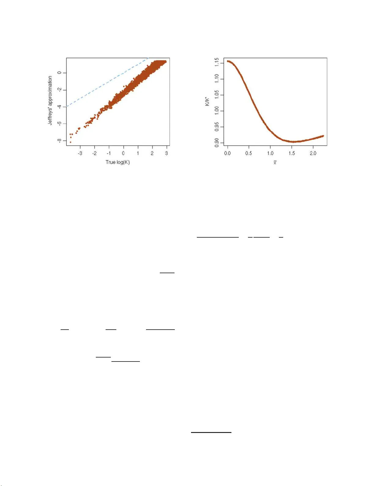
Statistic al Scienc e 2009, V ol. 24, No. 2, 141– 172 DOI: 10.1214 /09-STS284 c  Institute of Mathematical Statisti cs , 2009 Ha rold Jeﬀreys’s Theo ry of Probabilit y Revisited Christian P . Rob ert, Nicolas Chopin and Judith Rousseau Abstr act. Published exactly sev ent y y ears ago, Jeﬀreys’s The ory of Pr ob ability (1939) has had a unique impact on the Ba y esian commu- nit y and is now considered to b e one of the main classics in Ba y esian Statistics as w ell as the initiator of th e ob jectiv e Bay es sc ho ol. In par- ticular, its adv an ces on th e deriv ation of n oninformativ e p riors as wel l as on the scaling of Ba y es factors h a v e had a lasting impact on the ﬁeld. Ho wev er, the b o ok r eﬂ ects the c haracteristics of th e time, esp ecia lly in terms of mathematical rigor. In this pap er we p oin t out the fundamen- tal asp ects of this reference wo rk, esp ecially the th orou gh co ve rage of testing pr oblems and the construction of b oth estimation and testing noninformativ e pr iors based on functional div ergences. Ou r m a jor aim here is to help mod ern readers in navi gating in th is diﬃcult text and in concen trating on passages that are still relev ant to day . Key wor ds and phr ases: Ba yesia n f oundations, noninformativ e prior, σ -ﬁnite measure, Jeﬀreys’s prior, Kullbac k div ergence, tests, Bay es fac- tor, p -v alues, go o dn ess of ﬁt. Christian P. Ro b ert is Pr ofessor of St atist ics, Applie d Mathematics Dep artment , Universit´ e Paris Dauphine and He ad of the Statist ics L ab or atory, Cent er for R ese ar ch in Ec onomics and Statistics (CREST), National Institu te for S tatistics and Ec onomic Stu dies (INSEE), Paris, F r anc e e-mail: xian@c er emade.dauphi ne.fr . H e was the Pr esident of ISBA (International So ciety for Bayesian Analysi s) for 2008. Nic olas Chopin is Pr ofessor of S t atistics, ENSAE (National Scho ol for Statistics and Ec onomic A dministr ation), and Memb er of the S tatistics L ab or atory, Center for Re se ar ch in Ec onomics and Statistics (CREST), National In stitute for Statist ics and Ec onomic Studies (INSEE), Paris, F r anc e e-mail: nic olas.chopin@ensae.f r . Judith R ousse au is Pr ofessor of Statistics, Applie d Mathematics Dep artment, Universit´ e Paris Dauphine, and Memb er of t he Statistics L ab or atory, Center for Rese ar ch in Ec onomics and Statistics (CREST), N ational Institu te for Statistics and Ec onomic Stu dies (IN SEE), Paris, F r anc e e-mail: r ousse au@ensae.fr . 1 Discussed in 10.1214 /09-STS284E , 10.1214 /09-STS284D , 10.1214 /09-STS284A , 10.1214 /09-STS284F , 10.1214 /09-STS284B , 10.1214 /09-STS284C ; rejoinder at 10.1214 /09-STS284REJ . 1. INTRODUCTION The the ory of pr ob ability makes it p ossible to r esp e ct the gr e at men on whose shoulders we stand. H. Jeffr eys , The ory of Pr ob ability , Section 1.6. F ew Ba y esian b o oks other than The ory of Pr ob a- bility are so often cited as a foundational text. 1 This b o ok is righ tly considered as the principal reference in mo dern Ba y esian statistics. Among other inno v a- tions, The ory of P r ob ability states the general princi- ple for d eriving noninformative pr iors from the sam- pling distribu tion, using Fisher inform ation. It also This is an electronic r eprint o f the original ar ticle published by the Institute of Mathematical Statistics in Statistic al S cienc e , 2009, V ol. 24, No. 2, 141 –172 . This reprint diﬀers from the origina l in pagina tion and t yp ogr aphic detail. 1 Among th e “Bay esian classics,” only Sav age ( 1954 ), DeG- root ( 1970 ) and Berger ( 1985 ) seem to get more citations than Jeﬀreys ( 1939 , 1948 , 1961 ), the more recen t b o ok by Bernardo and Smith ( 1994 ) coming fairly close. The homonymous The- ory of Pr ob abili ty by d e Finetti ( 1974 , 1975 ) gets quoted a third as muc h ( Sour c e: Go o gle Scholar ). 1 2 C. P . ROBER T, N . CHOPIN AND J. ROUSSEAU prop oses a clear pro cessing of Ba ye sian testing, in- cluding the dim en sion-free scaling of Ba yes factors. This comprehens iv e treatmen t of Ba yesia n in ference from an ob jectiv e Ba ye s p ersp ectiv e is a ma jor inno- v ation for the time, and it h as certainly contributed to the adv ance of a ﬁeld that wa s then sub mitted to sev ere criticisms b y R. A. Fisher (Aldric h, 2008 ) and others, and w as in d anger of b eco ming a feature of the past. As p ointe d out by Zellner ( 1980 ) in h is in- tro duction to a volume of essa ys in honor of Harold Jeﬀreys, a f u ndamenta l strength of The ory of Pr ob- ability is its aﬃrmation of a unitarian principle in the statistical pro cessing of all ﬁelds of science. F or a 21st ce ntury r eader, Jeﬀreys’s The ory of Pr ob ability is nonetheless pu zzling for its lac k of formalism, includ ing its diﬃculties in handling im- prop er priors, its reliance on in tuition, its long de- bate ab out the nature of probabilit y , and its re- p eated attempts at ph ilosophical justiﬁcations. The title itself is misleading in that there is abs olutely no exp osition of the mathematical b ases of probabil- it y theory in the sense of Billingsley ( 1986 ) or F eller ( 1970 ): “Theory of Inv erse Probabilit y” would h a ve b een more accurate. In other w ords, the st yle of the b o ok app ears to b e b oth v er b ose and often v ague in its mathematical foundations for a mo dern reader. 2 (Goo d, 1980 , also ac knowledge s that many passages of the b o ok are “obscure.”) It is thus diﬃcult to ex- tract from this dense text the pr inciples th at made The ory of Pr ob ability the reference it is no w ada ys. In this p ap er we end eav or to r evisit the b o ok fr om a Bay esian p ersp ectiv e, in order to separate f ounda- tional prin ciples from less relev ant parts. This review is neither a historical nor a critical exercise: while conscious that The ory of P r ob abil- ity reﬂects the id iosyn crasies b oth of the scien tiﬁc ac h ievemen ts of the 1930’s—with, in particular, the emerging formalization of Pr obabilit y as a branc h of Mathematics against the ongoing debate on the na- ture of probabilities—and of Jeﬀreys’s bac kground— as a geophysicist —, w e aim rather at providing the mo dern reader with a reading guide, fo cusing on the pioneering adv ances made by this b o ok. Parts that corresp ond to the lac k (at the time) of analytical (lik e m atrix algebra) or numerical (lik e sim ulation) to ols and their su bstitution by appro ximation de- vices (that are not used an y longer, even though 2 In order to keep readabilit y as high as p ossible, we shall use mo dern notation whenever th e original notation is either unclear or inconsistent, for example, Greek letters for param- eters and roman letters for observ ations. they ma y b e surpr isingly accurate), and parts that are link ed with Ba y esian p ersp ectiv es will b e co v ered ﬂeetingly . Thus, when p oin ting out notions that ma y seem outdated or ev en mathematically unsou n d by mo dern standard s, our only aim is to help the mo d- ern reader stroll p ast them, and we ap olog ize in ad- v ance if , despite our int ent , our tone seems ov erly presump tuous: it is rather a reﬂection of our igno- rance of the current conditions at the time since (to b orrow from th e ab o ve qu ote whic h m ay s ound it- self someho w p r esumptuous) w e stand resp ectfully at the feet of this giant of Ba ye sian S tatistics. The p lan of the p ap er follo ws The ory of Pr ob abil- ity linearly by allocating a section to eac h c hapter of the b o ok (App endices are only m en tioned through- out the pap er). Section 10 con tains a brief conclu- sion. No te that, in the follo wing, words, sentences or passages quoted from The ory of Pr ob ability are written in italics with no precise indication of their lo cation, in order to kee p the st yle as ligh t as p os- sible. W e also stress that our review is b ased on the third edition of The ory of P r ob ability (Jeﬀreys, 1961 ), since this is b oth the most matured and the most a v ailable version (thr ough th e last rep r in t by Oxford Universit y Press in 1998). Conte mp orary re- views of The ory of P r ob ability are f ound in Go o d ( 1962 ) and Lindley ( 1962 ). 2. CHAPT ER I: FUND AMENT AL NOTIONS The p osterior pr ob abilities of the hyp otheses ar e pr op ortiona l to the pr o ducts of the prior pr ob abilities and the likeliho o ds. H. Jeffr eys , The ory of Pr ob ability , Section 1.2. The ﬁrst chapter of The ory of Pr ob ability sets gen- eral goals for a c oher ent theory of ind uction. More imp ortantl y , it pr op oses an axiomatic (if sligh tly tautologi cal) deriv ation of prior distributions, wh ile justifying this approac h as coheren t, compatible with the or dinary pr o c ess of le arning and allo wing for the incorp oration of imprecise information. It also r ec- ognizes the fund amen tal prop ert y of coherence when up d ating p osterior distribu tions, since they c an b e use d as the prior pr ob ability in taking into ac c ount of a fu rther set of data . Despite a st yle that is often diﬃcult to p enetrate, this is thus a ma jor chapter of The ory of Pr ob ability . I t will also b ecome clearer at a later stage that the principles exp osed in this c hap- ter corresp ond to th e (mo dern) notion of ob jectiv e Ba yes inference: despite men tions of p rior probabil- ities as reﬂections of p rior b elief or existing pieces of THEOR Y OF PROBABILITY REVIS ITED 3 information, The ory of Pr ob ability remains strictly “ob jectiv e” in that prior distributions are alw a ys de- riv ed analytically from sampling distributions and that all examples are treated in a nonin formativ e manner. One ma y ﬁn d it sur p rising that a p hysi- cist like Jeﬀreys d o es not emphasise the app eal of sub jectiv e Ba y es, that is, the ability to tak e in to ac- coun t gen u ine prior information in a principled w ay . But this is in line with b oth his pr edecessors, in- cluding Laplace and Ba yes, and their use of u niform priors and his main ﬁeld of study th at he p erceiv ed as ob jectiv e (Lind ley , 2008, pr iv ate comm u nication), while one of the main app eals of The ory of Pr ob abil- ity is to pr o vide a general and coherent framew ork to derive ob jectiv e p riors. 2.1 A P hilosophical Exercise The c hapter starts in Section 1.0 with an epis- temologi cal discussion of th e nature of (statistical) inference. S ome sections are quite puzzling. F or in- stance, the example that the kin ematic equation for an ob ject in free-fall, s = a + ut + 1 2 g t 2 , cannot b e de duc e d from observ ations is used as an argumen t against dedu ction un der the reasoning that an inﬁn ite n umb er of fu nctions, s = a + ut + 1 2 g t 2 + f ( t )( t − t 1 ) · · · ( t − t n ) , also apply to d escrib e a free fall observed at times t 1 , . . . , t n . The limits of the epistemological discus- sion in those early pages are illustrated b y the in- tro duction of Oc kham’s razor ( the choic e of the sim- plest law that ﬁts the fact ), as the meaning of wh at a simplest law can b e remains un clear, and the sec- tion lac ks a clear (ob jectiv e) argument in motiv ating this c h oice, b esides common sense, while the d iscu s- sion ends u p with a someho w parado xical statemen t that, since de ductive lo gic pr ovides no e xplanation of the choic e of the simplest law , this is pr o of that de ductive lo gic is gr ossly inade quate to c over scien- tiﬁc and pr actic al r e quir ements . On the other h and, and f rom a statistician’s narro we r p ers p ectiv e, one can re-int erpr et this gra vit y example as p ossibly the earliest discussion of the conceptual diﬃculties asso- ciated with m o del c hoice, whic h are still n ot ent irely resolv ed to da y . In that r esp ect, it is quite fascinat- ing to see this discuss ion app ear so early in the b o ok (third page), as if Jeﬀreys had p erceiv ed ho w imp or- tan t this deb ate w ould b ecome later. Note that, mayb e du e to th is very call to Oc kham, the later Ba yesian literature ab oun ds in references to Ockham’s r azor with little formalization of this principle, ev en though Berge r and Jeﬀerys ( 1992 ), Balasubramanian ( 1997 ) and MacKa y ( 2002 ) dev elop elab orate approac hes. In p articular, the deﬁnition of the Ba y es factor in Section 1.6 can b e seen as a partial implementa tion of Oc kham’s razor when set- ting th e prob ab ilities of b oth mo dels equal to 1 / 2. In th e b eginning of his Chapter 28, entitl ed Mo del Choic e and Oc c am’s R azor , MacKa y ( 2002 ) argues that Ba y esian inference em b o dies Ockham’s razor b ecause “simple” mo dels tend to pro du ce m ore pre- cise pred ictions and, th us, when the data is equ ally compatible with s ev eral mo d els, the simplest one will end up as the most p robable. Th is is generally true, ev en though there are some coun terexamples in Ba y esian nonp arametrics. Ov erall, w e nonetheless feel that this p art of The- ory of Pr ob ability could b e skipp ed at ﬁrst r ead- ing as less relev ant for Ba y esian stud ies. In p articu- lar, the opp osition b et wee n mathematical dedu ction and s tatistical induction do es n ot app ear to carry a strong argumen t, ev en th ou gh the d istinction n eeds (needed?) to b e made for mathemati cally orien ted readers unf amiliar with statistics. How ev er, from a historical p oin t of view, this opp osition must b e con- sidered against the then-ongoing debate ab out the nature of indu ction, as illustrated, for instance, by Karl P opp er’s articles of this p eriod ab out th e logi- cal imp ossibilit y of induction (Popp er, 1934 ). 2.2 F oundational Principles The text b ecomes more fo cused wh en d ealing with the construction of a the ory of infer enc e : w hile some notions are y et to b e deﬁned, includ in g the p erv asiv e evidenc e , sente nces lik e infer enc e involves in its very natur e the p ossibility that the alternative chosen as the most likely may in fact b e wr ong are in line w ith our cu rrent in terpretation of mo deling and obvio usly with the Ba yesia n paradigm. In Section 1.1 Jeﬀreys sets u p a coll ection of p ostulates or rules th at act lik e axioms for his theory of in f erence, some of which require later explanations to b e fu lly und ersto o d: 1. Al l hyp otheses must b e explicitly state d and the c onclusions must fol low fr om the hyp otheses : what ma y ﬁrst sound lik e an obvious scienti ﬁc principle is in fact a leading c h aracteristic of Ba y esian statis- tics. While it seems to op en a whole range of new 4 C. P . ROBER T, N . CHOPIN AND J. ROUSSEAU questions—“T o wh at extent m ust we deﬁn e our b e- lief in the statistical mo dels used to build our in- ference? Ho w can a un ique conclusion stem f rom a giv en m o del and a giv en set of observ ations?”—and while it ma y sound f ar to o generic to b e u s eful, we ma y in terpret this statemen t as setting the wo rking principle of Ba yesia n decision theory: giv en a p rior, a samp ling distrib u tion, an observ ation and a loss function, there exists a s in gle decision p ro cedure. In contrast, the frequentist theories of Neyman or of Fisher require the c hoice of ad ho c p ro cedures, whose (go o d or b ad) prop erties they later analyze . But this may b e a far-fetc h ed inte rpr etation of th is rule at this stage ev en th ough the commen t will ap- p ear m ore clearly later. 2. The the ory must b e self-c onsistent . The state- men t is someho w a rep etition of the p revious ru le and it is only later (in Section 3.10) that its mean- ing b ecomes clea rer, in connection with the in tro- duction of Jeﬀreys’s n oninformativ e priors as a self- con tained principle. Consistency is nonetheless a dom- inan t feature of the b o ok, as illustrated in Section 3.1 with the r ejection of Haldane’s prior. 3 3. Any rule must b e applic able in pr actic e . T his “rule” do es n ot seem to carry an y w eigh t in prac- tice. In addition, the explicit proh ib ition of esti- mates b ased on imp ossible exp eriments sounds im- plemen table only through d eductiv e argumen ts. But this leads to the exclusion of rules based on fr e- quency argum ents and, as suc h, is fundamenta l in setting a Ba y esian framework. Alternativ ely (and this is another in terpretation), this constraint sh ou ld b e w orded in more formal terms of the measur abilit y of pro cedu res. 4. The the ory must pr ovide explicitly for the p os- sibility tha t infer enc es made by it may turn out to b e wr ong . This is b oth a fu ndamenta l asp ect of sta- tistical inference and an indication of a surprising view of inf erence. Ind eed, ev en when conditioning on the mo del, inference is n ever right in the sen s e that a p oin t estimate rarely giv es the true answ er. It ma y b e that J eﬀreys is solely thinking of sta- tistical testi ng, in w hic h ca se the right fulness of a decision is necessarily conditional on the truthful- ness of th e corresp ond ing mo del and thus dub ious. A more relativ e (or more precise) statement w ould 3 Consistency is th en to b e understo o d in th e we ak sense of inv arian t u n der reparameterization, which is a usual argumen t for Jeﬀreys’s principle, not in terms of asymptotic conv ergence prop erties. ha v e b een m ore adequate. But, from reading fur- ther (as in Section 1.2), it app ears that this rule is to b e u ndersto o d as the found ational p r inciple ( the chief c onstructive rule ) for deﬁning prior distribu - tions. While this is certainly not clear at this stage, Ba yesia n inference do es indeed pro vide for the p os- sibilit y that the mo del u nder study is n ot correct and for the un reliabilit y of the resu lting inference via a p osterior p robabilit y . 5. The the ory must not deny any empiric al pr op o- sition a priori . Th is principle remains unclear w h en put in to p r actice. If it is to b e und ersto o d in the sense of a physical theory , there is no reason w hy some empirical prop osition could not b e excluded from the start. If it is th e sense of an inferen tial theory , then the statemen t w ould require a b etter deﬁnition of empiric al pr op osition . But Jeﬀr eys us- ing the epithet a priori seems to imply that the prior distribution corresp onding to the the ory must b e as inclusiv e as p ossib le. This certainly makes sense as long as prior inform ation d o es not exclude p arts of the parameter space as, for ins tance, in Physics. 6. The numb er of p ostulates should b e r e duc e d to a minimum . This ru le soun ds lik e an em b edd ed Ock- ham’s razor, bu t, more p ositiv ely , it can also b e in - terpreted as a call for noninformative priors. Once again, the v agueness of the w ording op ens a w ide range of in terpretations. 7. The the ory ne e d not r epr esent thought-pr o c esses in details, but should agr e e with them in outline . This v ague p rinciple could b e an attempt at rec- onciliating statistic al theories, bu t it do es not give clear dir ections on ho w to pro ceed. In the ligh t of Jeﬀreys’s arguments, it could rather signify that the construction of prior distributions cannot exactly re- ﬂect an actual constru ction in real life. Since a non- informativ e (or “ob jectiv e”) p ersp ectiv e is adopted for most of the b o ok, this is m ore lik ely to b e a pre- liminary argum ent in fa v or of this line of thought. In Section 1.2 th is rule is inv ok ed to derive the (prior) ordering of even ts. 8. An obje ction c arries no weight if [it] would in- validate p art of pur e mathematics . This r u le grounds The ory of P r ob ability within mathematics, w hic h ma y b e a n ecessary reminder in th e spirit of the time (where some we re attempting to disso ciate statis- tics from mathematics). The next paragraph discusses the notion of pr ob- ability . Its in terest is mostly historical: in the early 1930’s, the axiomatic d eﬁnition of probabilit y based THEOR Y OF PROBABILITY REVIS ITED 5 on Kolmogoro v’s axioms w as not y et univ ersally ac- cepted, and there w ere s till attempts to base this deﬁnition on limiting prop erties. In particular, Leb esgue inte gration w as not part of the undergrad- uate curriculum till th e late 1950’s at either Cam- bridge or Oxford (Lindley , 2008, pr iv ate communi- cation). This d ebate is n o longer r elev an t, and the current theory of probabilit y , as derived from mea- sure theory , do es not b ear further d iscussion. This also remov es the am biguity of constructing obje ctive pr ob abilities as derived from actual or p ossible ob- servations . A probability mo del is to b e understo od as a mathematical (and thus un ob jectionable) con- struct, in agreemen t with Ru le 8 ab o ve. Then follo w s (still in Section 1.1) a rather long debate on c ausality versus determinism . While the principles stated in those pages are quite accept- able, the discussion only u ses the most b asic concept of determinism , namely , that id entical causes giv e iden tical eﬀects, in the sense of Laplace. W e th us agree with Jeﬀreys that, at th is lev el, the principle is useless , but the same paragraph actually lea ve s us quite confused as to its real purp ose. A lik ely ex- planation (Lin dley , 2008, p ersonal comm unication) is that Jeﬀreys str esses the inevitabilit y of probabil- it y statemen ts in S cience: (measurement) errors are not mistak es but part of the pictur e. 2.3 Prio r Distributions In S ection 1.2 Jeﬀreys introd uces the notion of prior in an indirect wa y , by consid ering that th e probabilit y of a prop osition is alw a ys cond itional on some data and that the o ccurrence of new items of information ( new evidenc e ) on this prop osition sim- ply up dates th e av ail able data. This is slight ly con- trary to ou r cur ren t wa y of deﬁnin g a prior distri- bution π on a parameter θ as the information av ail - able on θ prior to the obser v ation of the data, b ut it simply con veys the f act that the pr ior distribu- tion must b e d eriv ed f rom some prior items of in- formation ab out θ . As p ointed out by Jeﬀreys, this also allo ws for the co existence of pr ior distribu tions for diﬀerent exp erts within the same pr obabilistic framew ork. 4 In the sequel all statemen ts will, how- ev er, condition on the same d ata. The follo wing paragraphs deriv e stand ard math- ematical logic axioms that directly follo w from a 4 Jeﬀreys seems to further note th at the same conditioning applies for the mod el of reference. formal (mo d ern) deﬁn ition of a probab ility distri- bution, with th e pro vision that this probability is alw a ys conditional on the same d ata. This is also reminiscen t of the deriv ation of the existence of a prior distribution from an ordering of prior pr oba- bilities in DeGroot ( 1970 ), bu t the discussion ab ou t the arbitrary ranking of pr ob ab ilities b et ween 0 and 1 may sou n d anecdotal to d a y . Note also that, from a m athematical p oint of view, deﬁning only condi- tional pr obabilities lik e P ( p | q ) is someho w sup erﬂu- ous in that, if the conditioning q is to remain ﬁxed, P ( ·| q ) is a regular probabilit y d istribution, wh ile, if q is to b e up dated into q r , P ( ·| q r ) can b e deriv ed from P ( ·| q ) b y Ba y es’ theorem (whic h is to b e in - tro duced later). Therefore, in all cases, P ( ·| q ) ap- p ears lik e the r eference probability . At some stage, while stating that the probabilit y of the sure ev ent is equal to one is merely a conv enti on, J eﬀr eys indi- cates that, when expressing ig nor anc e over an inﬁ- nite r ange of values of a quantity, it may b e c onve- nient to use ∞ instead. Clearly , this pav es the wa y for the introdu ction of improp er priors. 5 Unfortu- nately , the con ven tion an d the m otiv ation ( to ke ep r atios for ﬁnite r anges determinate ) do not seem correct, if in tune w ith the p ersp ectiv e of the time (see, e.g., Lhoste, 1923 ; Bro emeling and Bro emel- ing, 2003 ). Notably , setting all ev ents inv olving a n inﬁnite range with a probabilit y equal to ∞ seems to restrict the abilities of th e theory to a far ex- ten t. 6 Similar to Laplace, Jeﬀreys is more us ed to handling equal probabilit y ﬁn ite sets than con tin u- ous s ets and the extension to con tin uous settings is unortho d o x, using, for instance, Dedekind’s sections and putting sev eral m eanings under the notation dx . Giv en the con v oluted deriv ation of conditional prob - abilities in th is cont ext, the b ook states th e p ro du ct rule P ( q r | p ) = P ( q | p ) P ( r | q p ) as an axiom, rather than as a consequence of the basic p robabilit y ax- ioms. It leads (in Section 1.22) to Ba yes’ theorem, 5 Jeﬀreys’s The ory of Pr ob abili ty strongly d iﬀers from the earlier Scientiﬁc Infer enc e ( 1931 ) in this respect, the latter b e- ing rather dismissiv e of the mathematical diﬃculty: T o make this inte gr al e qual to 1 we should ther efor e have to include a zer o f actor unless very smal l and very lar ge values ar e ex- clude d. This do es app e ar to b e the c ase (S ection 5.43 , page 67). 6 This d iﬃculty with h an d ling σ -ﬁn ite measures and contin- uous v ariables will b e recurrent throughou t th e bo ok: Jeﬀreys does not seem to be adverse to normalizing an improper dis- tribution by ∞ , even th ough the corresp onding deriv ations are n ot meaningful. 6 C. P . ROBER T, N . CHOPIN AND J. ROUSSEAU namely , that, for all ev en ts q r , P ( q r | pH ) ∝ P ( q r | H ) P ( p | q r H ) , where H d enotes the information available and p a set of observations . In this (mo der n ) format P ( p | q r H ) is iden tiﬁed as Fisher likeli ho o d and P ( q r | H ) as the prior p robabilit y . Ba yes’ theorem is d eﬁned as the principle of inverse pr ob ability a nd only for ﬁ nite sets, rather than for measures. 7 Ob viously , the gen- eral v ersion of Ba ye s’ theorem is u sed in the sequ el for con tinuous parameter spaces. Section 1.3 represen ts one of the few fora ys of the b o ok into the r ealm of decision theory , 8 in con- nection with Laplace’s notions of mathematical and moral exp ectatio ns, and with Bernoulli’s Saint P e- tersburg parado x, bu t there is no recognition of the cen tral role of the loss fun ction in deﬁning an opti- mal Bay es rule as formalized later by W ald ( 1950 ) and Raiﬀa and Schlaifer ( 1961 ). The attribution of a decision-theoretic backg round to T. Ba ye s himself is surprising, since there is not anything close to the notion of loss or of b eneﬁt in Ba ye s’ (1763) origi- nal p ap er. W e nonetheless ﬁ nd there the seed of an idea later deve lop ed in Rubin ( 1987 ), among oth- ers, that pr ior and loss function are indistinguish- able. [Section 1.8 brieﬂy re-en ters this p ersp ectiv e to p oin t ou t that (p osterior) exp ectat ions are often nowher e ne ar the actual v alue of th e random quan- tit y .] The n ext section (Section 1.4) is im p ortan t in that it tac k les for the ﬁrst time the iss u e of nonin- formativ e priors. When the n umber of alternativ es is ﬁnite, Jeﬀreys picks the uniform prior as h is non- informativ e prior, follo w ing Laplace’s Principle of Insuﬃcient R e ason . The diﬃculties asso ciated w ith this c h oice in con tin uous settings are not mentio ned at this stage. 2.4 Mo re Axiomat ics and Som e A symptotics Section 1.5 attempts an axiomatic deriv ation that the Ba y esian prin ciples just stated follo w the rules 7 As noted by Fien b erg ( 2006 ), the adjectiv e term “Ba yesia n” had not yet app eared in th e statistical literature by the time The ory of Pr ob abil ity was published, and Jeﬀreys stic ks to the 19th century denomination of “in verse probabil- it y .” The adjective can b e t raced back to either Ronald Fisher, who u sed it in a rather derogatory meaning, or to Abraham W ald, who gav e it a more complimentary meaning in W ald ( 1950 ). 8 The reference p oint estimator advocated by Jeﬀreys (if any) seems to b e the maximum a p osterior i (MAP) estimator, even though he stated in his discussion of Lind ley ( 1953 ) that he depr e c ate d the whol e ide a of picking out a unique estimate . imp osed earlier. This part do es not bring m uch n o v- elt y , once the fu n dament al pr op erties of a proba- bilit y distribution are stated. This is basically the purp ose of this section, where earlier “Axioms” are c h ec k ed in terms of the p osterior pr ob ab ility P ( ·| pH ). A reassur in g consequence of this deriv ation is that the us e of a p osterior p robabilit y as the basis for inference cannot lead to inconsistency . The use of the p osterior as a n ew p r ior f or f u ture observ ations and the corresp onding learning prin ciple are devel - op ed at th is stage. Th e d ebate ab out th e c h oice of the pr ior distrib u tion is p ostp oned till later, wh ile the issue of the inﬂu ence of this prior distribution is d ism issed as ha ving v e ry little diﬀe r enc e [on] the r esults , whic h needs to b e quanti ﬁed, as in the qu ote b elo w at the b eginning of Section 5. Giv en the informal appr oac h to (or rather with- out) measure theory adopted in The ory of Pr ob abil- ity , the study of the limiting b eha vior of p osterior distributions in Section 1.6 do es not pr ovide muc h insigh t. F or instance, the fact that P ( q | p 1 · · · p n H ) = P ( q | H ) P ( p 1 | H ) P ( p 2 | p 1 H ) · · · P ( p n | p 1 · · · p n − 1 H ) is sh o w n to indu ce that P ( p n | p 1 · · · p n − 1 H ) conv erges to 1 is not particularly su rprising, although it relates to Laplace’s p rinciple that r ep e ate d veriﬁc ations of c onse quenc es of a hyp othesis wil l make it pr actic al ly c ertain that the next c onse quenc e wil l b e veriﬁe d . I t w ould ha ve b een equally interesting to fo cus on cases in which P ( q | p 1 · · · p n H ) goes to 1. The end of Section 1.62 in tro du ces some quan ti- ties of interest, such as the distinction b et wee n esti- mation problems and signiﬁcance tests, b ut with n o clear guideline: when comparin g mo dels of complex- it y m (this quan tit y b eing only deﬁ ned for diﬀeren- tial equations), J eﬀr eys su ggests using prior prob- abilities that are p enalized b y m , such as 2 − m or 6 /π 2 m 2 , the motiv ation for th ose sp eciﬁc v alues b e- ing that the corresp on d ing series con verge . Pe nal- ization by the mo del complexity is quite an in ter- esting id ea, to b e formalized later b y , for example, Rissanen ( 1983 , 1990 ), but Jeﬀreys s omehow kills this id ea b efore it is hatc hed by p ointing out the diﬃculties w ith the deﬁ n ition of m . Instead, Jeﬀreys switc hes to a completely diﬀerent (if paramoun t) topic by deﬁ n ing in a f ew lines the Ba yes factor for testing a p oint null hypothesis, K = P ( q | θ H ) P ( q ′ | θ H ) . P ( q | H ) P ( q ′ | H ) , THEOR Y OF PROBABILITY REVIS ITED 7 where θ d enotes the data. He suggests using P ( q | H ) = 1 / 2 as a d efault v alue, except f or sequences of em- b edd ed hyp otheses for whic h h e suggests P ( q | H ) P ( q ′ | H ) = 2 , presumably b ecause the series with leading term 2 − n is con v erging. Once again, the rather quic k co ve rage of this ma- terial is someho w frustr ating, as fur ther j u stiﬁca- tions would ha ve b een n ecessary for th e c hoice of the constan t and so on. 9 Instead, the chapter con- cludes with a discussion of the distinction b et wee n “idealism” and “realism” th at can b e skipp ed for most pu rp oses. 3. CHAPTER I I: DIRECT PROBA BILITIES The whole of the information c ontaine d in the observations that is r e levant to the p osterior pr ob abilities of diﬀer ent hyp otheses is summe d up in the values that they give to the likeliho o d. H. Jeffr eys , The ory of Pr ob ability , Section 2.0. This chapter is certainly th e least “Ba yesian” c h ap - ter of the b o ok, since it co v ers b oth the standard sampling d istributions and some equally standard probabilit y results. It s tarts with a r eminder that the principle of inverse pr ob ability c an b e state d in the form Posterior Pr ob ability ∝ Prior Pr ob ability · Like liho o d , th us rephr asing Bay es’ theorem in terms of the lik e- liho o d and w ith the p rop er indication that the r el- evant informa tion c ontaine d in the observa tions is summarized b y the lik eliho od ( suﬃci e ncy will b e men tioned later in S ection 3.7). Then follo ws (still in S ection 2.0) a long paragraph ab out the ten ta- tiv e nature of mo dels, concludin g that a statistica l mo del must b e made part of the pr ior inf orm ation H b efore it can b e tested against th e observ ations, whic h (presumably) r elates to the fact that Bay esian 9 Similarly , the argumen t against philosophers that mai n- tain that no metho d b ase d on the the ory of pr ob ability c an give a (... ) non-zer o pr ob abili ty to a pr e ci se value against a c ontin- uous b ackgr ound is not convincing as stated. The distinction b etw een zero measure even ts and mixture priors in cluding a Dirac mass shou ld hav e b een b ett er explained, since this is the b asis for Ba yesia n p oint-null t esting. mo del assessment must inv olve a descrip tion of the alternativ e(s) to b e v alidated. The main bulk of the chapter is about sampling distributions. Section 2.1 in tro du ces binomial and h yp ergeome tric distributions at length, includin g th e in teresting problem of deciding b et ween b in omial v ersus negativ e binomial exp erimen ts when faced with th e outcome of a su rv ey , u sed later in the de- fence of the Likelihoo d Pr inciple (Berger and W olpert, 1988 ). Th e description of the b inomial conta ins th e equally interesting r emark that a giv en coin rep eat- edly thro wn will sho w a bias to w ard head or tail due to the w ear, a remark later exploited in Diaconis and Ylvisak er ( 1985 ) to justify the u se of mixtur es of conjugate pr iors. Bernoulli’s v ers ion of the Cen tral Limit theorem is also recalled in this section, with no particular app eal if one considers that a m o d- ern S tatistics cour se (see, e.g., Casella and Berger, 2001 ) w ould ﬁ r st start with the p r obabilistic bac k- ground. 10 The Poisson distribu tion is ﬁrst introd uced as a limiting distribution for the binomial distribution B ( n, p ) when n is large and np is b oun ded. (Connec- tions with radioactiv e disin tegration are men tioned afterw ard.) Th e n orm al d istribution is prop osed as a large samp le app ro ximation to a sum of Bernoulli random v ariables. As for the other distr ib utions, there is some attempt at jus tifyin g th e use of the normal d istribution, as well as [wh at we ﬁn d to b e] a confu sing p aragraph ab out the “true” and “actual observ ed” v alues of the parameters. A long section (Section 2.3) expand s ab out the prop erties of Pea r- son’s distributions, then allo win g Jeﬀreys to intro- duce the negativ e b inomial as a mixtur e of Poisson distributions. The introd u ction of the biv ariate nor- mal distribu tion is similarly conv oluted, using ﬁrst binomial v ariates and second a limiting argument , and without resorting to matrix formalism. Section 2.6 attempts to introd uce cum ulativ e dis- tribution functions in a more formal manner, u sing the current three-step d eﬁnition, but again d ealing with limits in an inform al w a y . Rather coheren tly from a geophysici st’s p oin t of view, characte ristic functions are also co v ered in great d etail, includ in g connections with momen ts and the Cauch y d istr ibu- tion, as we ll as L´ evy’s inv ersion theorem. The main 10 In fact, some of t he statements in The ory of Pr ob ability that surroun d the statement of the Centra l Limit theorem are not in agreemen t with measure t heory , as, for instance, the confusion b etw een p oint wise and un iform conve rgence, and conv ergence in probabilit y and converg ence in distribution. 8 C. P . ROBER T, N . CHOPIN AND J. ROUSSEAU goal of using characte ristic functions seems nonethe- less to b e able to establish the Central Limit theo- rem in its fu ll generalit y (Section 2.664) . Rather surprisin gly for a Ba y esian reference b o ok and mostly in complete disconnection with the test- ing c hapters, the χ 2 test of goo dness of ﬁt is giv en a large and uncritical place within this b o ok, includ- ing an adjus tmen t for the degrees of f r eedom. 11 Ex- amples includ e the obvious indep endence of a r ect- angular con tingency table. The only criticism (Sec- tion 2.76) is fairly obscure in that it blames p o or p erforman ces of the χ 2 test on the fact that all d i- v ergences in the χ 2 sum are equally weig hte d. The test is n onetheless im p lemen ted in the most classi- cal manner, namely , that the hyp othesis is rejected if the χ 2 statistic is outside the standard in terv al. It is un clear from the text in Section 2.76 th at r e- jection would o ccur were the χ 2 statistic to o small, ev en though J eﬀreys righ tly add resses the issue at the end of Chapter 5 (Section 5.63). He also men- tions the n eed to coalesce small groups int o groups of size at least 5 with no f urther j u stiﬁcation. The c h apter concludes with similar uses of Student’s t and Fisher’s z tests. 4. CHAPTER I I I: ESTIMA TION PROBLEMS If we have no information r elevant to the actual value of the p ar ameter, the pr ob ability must b e chosen so as to expr ess the fact that we have none. H. Jeffr eys , The ory of Pr ob ability , Section 3.1. This is a ma jor c h apter of The ory of Pr ob abil- ity as it introd uces b oth exp onen tial families and the principle of Jeﬀreys noninformativ e priors. The main concepts are already present in the early sec- tions, includin g some in v ariance principles. T he pur - p ose of the c hapter is s tated as a p oin t estimation problem, w here obtaining th e pr ob ability distribu- tion of [the] p ar ameters, given the observations is the goal. Note that estimation is not to b e under- sto o d in the (mo dern?) sense of p oint estimation, that is, as a w a y to pr o duce n umerical sub s titutes for the tru e parameters that are based on the d ata, 11 Interestingly en ou gh , the parameters are estimated by minim um χ 2 rather th an eith er maximum likelihoo d or Ba yesian p oint estimates. This is, again, a reﬂection of the practice of th e time, coup led with the fact that most ap- proac hes are asymp totically indistinguishable. P osterior ex- p ectations are not at all advocated as Bay es (p oint) estima- tors in The ory of Pr ob ability . since the decision-theoretic p ersp ectiv e for bu ilding (p oint ) estimators is mostly missing f r om the b o ok (see Section 1.8 for a very brief remark on exp ecta- tions). Both Go o d ( 1980 ) and Lind ley ( 1980 ) stress this absence. 4.1 Noninfo rmative Pr iors of Fo rmer Da ys Section 3.1 sets th e principles f or selecting nonin- formativ e priors. Jeﬀreys r ecalls Laplace’s ru le that, if a parameter is real-v alued, its prior pr ob ability should b e taken as uniformly distribute d , w h ile, if this parameter is p ositiv e, the prior pr ob ability of its lo garithm should b e taken as uniformly distribute d . The motiv ation adv anced for using b oth priors is the invar ianc e principle , namely , the in v ariance of the prior selecti on under sever al diﬀer ent sets of p a- r ameters . At this stage , there is no recognition of a p oten tial problem with usin g a σ -ﬁnite measure and, in p articular, with th e fact that these pr iors are not probabilit y d istributions, but rather a sim- ple warning that these are formal rules expr essing ignor anc e . W e face the diﬃcult y men tioned earlier when considerin g σ -ﬁn ite m easures sin ce they are not p r op erly h andled at this s tage: w hen stating that one starts with any distribution of prior pr ob a- bility , it is not p ossible to in clude σ -ﬁn ite measures this w a y , except via the [incorrect] argument that a pr ob ability is mer ely a numb er and, thus, that the total weigh t can b e ∞ as w ell as 1: use ∞ inste ad of 1 to indic ate c ertainty on data H . Th e wrong in- terpretation of a σ -ﬁnite m easur e as a probabilit y distribution (and of ∞ as a “n umb er ”) then leads to imm ed iate paradoxes, such as the pr ior proba- bilit y of an y ﬁnite range b eing null, wh ich sound s inc onsistent with the statement that we know noth- ing ab out the parameter, b ut this results from an o ver-in terpr etation of the measure as a probabilit y distribution already p oin ted ou t by Lindley ( 1971 , 1980 ) and Kass and W asserman ( 1996 ). The argument for using a ﬂ at (Leb esgue) prior is based (a) on its use b y b oth Ba y es and Laplace in ﬁnite or compact settings, and (b ) on the argument that it correctly reﬂects the absence of prior knowl- edge ab out the value of the p ar ameter . A t this stage, no p oin t is made against it f or reasons related w ith the invarianc e principle —there is only one parame- terizatio n th at coincides with a unif orm prior—b ut Jeﬀreys already argues that ﬂat p riors cann ot b e used for signiﬁcance tests, b ecause they w ould al- w a ys reject the p oin t null hyp othesis. Even though Ba yesia n signiﬁcance tests, including Ba ye s factors, THEOR Y OF PROBABILITY REVIS ITED 9 ha v e not y et b een prop erly introdu ced, the notion of an inﬁ nite mass canceling a p oin t null hyp othesis is suﬃciently in tuitiv e to b e used at this p oint. While, ind eed, using an improp er prior is a ma- jor d iﬃ cu lt y w hen testing p oint n ull hyp otheses b e- cause it gives an inﬁn ite mass to the alternativ e (DeGroot, 1970 ), Jeﬀreys fails to id entify the prob- lem as such but rather b lames the ﬂat pr ior applie d to a p ar ameter with a semi- inﬁnite r ange of p os- sible values . He then go es on justifying the use of π ( σ ) = 1 /σ for p ositive parameters (replicating the argumen t of Lhoste, 1923 ) on the basis that it is in v ariant f or the c han ge of parameters  = 1 /σ , as w ell as any other p ow er, failing to recognize that other transforms that p r eserv e p ositivit y do not ex- hibit su c h an inv ariance. One has to ad m it, h o w ev er, that, from a physic ist’s p ersp ectiv e, p o wer trans- forms are more imp ortant than other mathematical transforms, such as arctan, b ecause they can b e as- signed meanin gfu l units of measurement, while other functions cannot. At least this seems to b e the spirit of the examples considered in The ory of Pr ob ability : Some metho ds of me asuring the char ge of an ele c- tr on g i ve e , others e 2 . There is a v ague indication that Jeﬀreys may also recognize π ( σ ) = 1 /σ as the scale group inv ariant measure, bu t this is un clear. An indefensible argu- men t follo ws, namely , that Z a 0 v n dv . Z ∞ a v n dv is only ind eterminate when n = − 1, whic h allo ws us to av oid con tr adictions ab out th e lac k of prior in- formation. Jeﬀreys ac kno wledges that this do es n ot solv e the problem since this c hoice imp lies that the prior “probabilit y” of a ﬁnite inte rv al ( a, b ) is then alw a ys null, but he av oids the diﬃcult y b y admit- ting that the probabilit y that σ falls in a particu- lar range is ze ro, b ecause zer o pr ob ability do es not imply imp ossibility . He also ac knowle dges that the invarianc e principle cannot encompass the whole range of transforms without b eing inc onsistent , but he nonetheless sticks to the π ( σ ) = 1 /σ prior as it is b e tter than the Bayes–L aplac e rule . 12 Once again, the argument su staining th e wh ole of Section 3.1 is 12 In b oth th e 19th and early 20th cen turies, th ere is a tra- dition within the not-yet-Ba yesian literature to go to extreme lengths in the justiﬁcation of a particular prior distribution, as if there existed one golden prior. See, for example, Broemeling and Bro emeling ( 2003 ) in this respect. incomplete since missing the fundamental issue of distinguishing p rop er fr om improp er p riors. While Haldane’s ( 1932 ) prior on probabilities (or rather on c hanc es as deﬁn ed in Section 1.7), π ( p ) ∝ 1 p (1 − p ) , is dismissed as to o extreme (and inc onsistent ), there is no discussion of the main d iﬃcult y with this prior (or with any other improp er pr ior asso ciated w ith a ﬁnite-supp ort sampling d istribution), w hic h is that the co rresp onding p osterior distribution is not d e- ﬁned when x ∼ B ( n, p ) is either equ al to 0 or to n (although Jeﬀreys concludes that x = 0 leads to a p oint mass at p = 0, due to the inﬁ n ite mass nor- malizatio n). 13 Instead, the corresp on d ing J eﬀreys’s prior π ( p ) ∝ 1 p p (1 − p ) is su ggested with little justiﬁcation against the (truly) uniform prior: we may as wel l u se the uniform dis- tribution . 4.2 Laplace’s Succession Rule Section 3.2 con tains a Ba yesian pr o cessing of Laplace’s succession ru le, which is an easy in tro d u c- tion given th at the parameter of the sampling dis- tribution, a hypergeometric H ( N , r ), is an integ er. The c h oice of a u niform prior on r , π ( r ) = 1 / ( N + 1), do es not requ ir e muc h of a discu s sion and the p os- terior distr ib ution π ( r | l , m, N , H ) =  r l   N − r m  .  N + 1 l + m + 1  is a v ailable in closed form , includ ing the normal- izing constan t. The p osterior predictiv e probabilit y that the next sp e cimen wil l b e of the same typ e is then ( l + 1) / ( l + m + 1) and more complex predictiv e probabilities can b e computed as w ell. As in earlier b o oks in v olving Laplace’s succession rule, th e sec- tion argues ab out its tru thfulness from a metaphys- ical p oin t of view (using classical argumen ts abou t 13 Jeﬀreys ( 1931 , 1937 ) do es address the problem in a clearer manner, stating t hat this is not serious, f or so long as the sample i s homo gene ous (me aning x = 0 , n ) the ex- tr eme values (me aning p = 0 , 1 ) ar e stil l admissible, and we do attach a hi gh pr ob abil ity to the pr op osition is of one typ e; while as so on as any exc eptions ar e known the extr eme values ar e c ompletely exclude d and no inﬁnity arises (Section 10.1, page 195). 10 C. P . ROBER T, N . CHOPIN AND J. ROUSSEAU the pr obabilities that the sun rising tomor r ow and that al l swans ar e white that alwa ys seem to b e as- so ciates themselv es w ith this topic) bu t, more in ter- estingly , it then mo v es to in tro du cing a p oin t mass on sp eciﬁc v alues of the parameter in p reparation for hyp othesis testing. Namely , follo w ing a renewed criticism of the uniform assessment via the fact that P ( r = N | l, m = 0 , N , H ) P ( r 6 = N | l = n, N , H ) = l + 1 N + 1 is to o small, J eﬀreys suggests setting aside a p ortion 2 k of the prior mass for b oth extreme v alues r = 0 and r = N . This is ind eed equiv alen t to u sing a p oint mass on the null hyp othesis of homogeneit y of the p opulation. While mixed samples are indep endent of the c hoice of k (since they exclud e those extreme v alues), a sample of the ﬁrst typ e with l = n lea ds to a p osterior p robabilit y r atio of P ( r = N | l = n, N , H ) P ( r 6 = N | l = n, N , H ) = n + 1 N − n k 1 − 2 k N − 1 1 , whic h leads to th e cr u cial qu estion of th e c hoice 14 of k . The ensuing discussion is not en tirely con vincing: 1 2 is to o lar ge , 1 4 is not unr e asonable [but] to o low in this c ase . The alternativ e k = 1 4 + 1 N + 1 argues that the classiﬁc ation of p ossibilities [is] as fol lows : (1) Population hom o gene ous on ac c ount of some gener al rule . (2) No gener al rule but extr eme values to b e tr e ate d on a level with others. T his pro- p osal is m ostly inte resting for its b earing on the con tin uous ca se, for, in the ﬁ nite case, it do es not sound logic al to put w eigh t on the n ull hypothesis ( r = 0 and r = N ) within the alternativ e, s ince this confuses the issue. (See Berger, Bernardo and Su n , 2009 , for a recen t r eapp raisal of this app roac h from the p oin t of view of reference priors.) Section 3.3 seems to extend L ap lace’s su ccession rule to th e case in wh ic h the class sample d c onsists of sever al typ es , but it actually d eals with the (m uc h more in teresting) case of Ba ye sian inferen ce for th e m ultinomial M ( n ; p 1 , . . . , p r ) distr ibution, when us- ing the Diric hlet D (1 , . . . , 1) distribution as a pr ior. Jeﬀreys r eco vers the Diric hlet D ( x 1 + 1 , . . . , x r + 1) 14 A p rior weigh t of 2 k = 1 / 2 is reasonable since it gives equal probabilit y to b oth hypotheses. distribution as the p osterior distribution and h e de- riv es the predictiv e p robabilit y that the next memb er wil l b e of the ﬁrst typ e as ( x 1 + 1)/ X i x i + r. There could b e some connections there with the ir- relev ance of alternativ e h yp otheses late r (in time) discussed in p olytomous regression m o dels (Gouri ´ eroux and Monfort, 1996 ), but they are we ll hidd en. In an y case, the Dirichlet distribution is not inv arian t to the in tro du ction of n ew t yp es. 4.3 P oisson Distribution The pro cessing of the estimation of the p ar ameter α of the Poisso n distribution P ( α ) is based on the [improp er] prior π ( α ) ∝ 1 /α , deemed to b e the c or- r e ct prior pr ob ability distribution for scale inv ariance reasons. Giv en n observ ations from P ( α ) with su m S n , Jeﬀreys r epro du ces Haldane’s ( 1932 ) deriv ation of the Gamma p osterior G a ( S n , n ) and he n otes that S n is a suﬃcient statistic , but do es not make a gen- eral p rop erty of it at this stage. (This is done in Section 3.7.) The alternativ e c hoice π ( α ) ∝ 1 / √ α will b e later justiﬁed in Section 3.10 n ot as Jeﬀreys’s (in v ariant ) prior but as leading to a p osterior deﬁn ed for all observ ations, wh ic h is not the case of π ( α ) ∝ 1 /α when x = 0 , a fact o verlook ed by Jeﬀreys. Note that π ( α ) ∝ 1 /α can nonetheless b e adv o cate d by Jeﬀreys on the groun d th at the P oisson pro cess deriv es from the exp onen tial distribution, for which α is a scale parameter: e − αt r epr esents the fr action of the atoms original ly pr esent that survive after time t . 4.4 No rmal Distribution When the sampling v ariance σ 2 of a normal mo del N ( µ, σ 2 ) is kno wn, the p osterior distribu tion asso ci- ated with a ﬂ at prior is correctly derived as µ | x 1 , . . . , x n ∼ N ( ¯ x, σ 2 /n ) (with the r ep eated diﬃcult y ab out the use of a σ -ﬁn ite measure as a probabilit y). Under the join t impr op er prior π ( µ, σ ) ∝ 1 /σ, the (marginal) p osterior on µ is obtained as a Stu- den t’s t T ( n − 1 , ¯ x, s 2 /n ( n − 1)) distribution, wh ile the marginal p osterior on σ 2 is an inv erse gamma I G (( n − 1) / 2 , s 2 / 2). 15 15 Section 3.41 also contains the interesting remark that, conditional on tw o observ ations, x 1 and x 2 , the p osterior THEOR Y OF PROBABILITY REVIS ITED 11 Jeﬀreys notices that, wh en n = 1, the ab o ve prior do es not lead to a prop er p osterior since π ( µ | x 1 ) ∝ 1 / | µ − x 1 | is not integ rable, but he concludes that the solution de g ener ates in the right way, wh ic h, w e supp ose, is mean t to say that there is not enough information in the data. But, without further for- malizatio n, it is a d elicate conclusion to make . Under the same noninformativ e pr ior, the p redic- tiv e densit y of a second sample with suﬃcient statis- tic ( ¯ x 2 , s 2 ) is found 16 to b e prop ortional to  n 1 s 2 1 + n 2 s 2 2 + n 1 n 2 n 1 + n 2 ( ¯ x 2 − ¯ x 1 ) 2  − ( n 1 + n 2 − 1) / 2 . A d ir ect conclusion is that this implies that ¯ x 2 and s 2 are dep end ent for the predictiv e, if indep endent given µ and σ , w hile the marginal predictiv es on ¯ x 2 and s 2 2 are Stud en t’s t and Fisher’s z , resp ectiv ely . Extensions to the prediction of m u ltiple future sam- ples with the same (Section 3.43) or with diﬀeren t (Section 3.44) means follo w without su rprise. In the latter case, giv en m s amp les of n r (1 ≤ r ≤ m ) nor- mal N ( µ i , σ 2 ) measurement s, the p osterior on σ 2 under the noninformativ e prior π ( µ 1 , . . . , µ r , σ ) ∝ 1 /σ is ag ain an in verse gamma I G ( ν / 2 , s 2 / 2) distribu- tion, 17 with s 2 = P r P i ( x r i − ¯ x r ) 2 and ν = P r n r , while the p osterior on t = √ n i ( µ i − ¯ x i ) /s is a Stu- den t’s t w ith ν degrees of freedom for all i ’s (no matter what the num b er of observ ations within this group is). Figure 1 represents th e p osteriors on the means µ i for the data set analyzed in this section on sev en sets of measur emen ts of the gra vit y . A para- probabilit y that µ is b etw een b oth observ ations is ex actly 1 / 2. Jeﬀreys attributes this prop erty to the fact that the scale σ is directly estimated from those tw o observa tions u nder a nonin- formativ e prior. Section 3.8 generalize s the observ ation to all location-scale families with med ian equal to th e lo cation. Oth - erwise, the p osterior probability is less than 1 / 2. Similarly , th e probabilit y t hat a th ird observ ation x 3 will b e b etw een x 1 and x 2 is equal to 1 / 3 und er the predictive. While Jeﬀreys giv es a pro of by complete integrati on, this is a direct consequ en ce of th e exchangeabili ty of x 1 , x 2 and x 3 . Note also that this is one of th e rare o ccurrences of a credible in terv al in the b o ok . 16 In the cu rrent 1961 edition, n 2 s 2 2 is mistakenly t yp ed as n 2 2 s 2 2 in equ ation (6) of S ection 3.42. 17 Jeﬀreys do es n ot use the term “inv erse gamma distribu- tion” but simply notes t h at this is a distribu t ion with a scale parameter that is given by a single set of tables (for a given ν ). He also n otices that th e distribution of the transform log( σ /s ) is closer to a n ormal distribu t ion than the original. Fig. 1. Seven p osterior distributions on the values of ac c el- er ation due to gr avity (i n cm/se c 2 ) at lo c ations in East Afric a when using a noninformative prior. graph in S ection 3. 44 con tains hints ab out hierar- c h ical Ba yes m o deling as a w a y of str engthening es- timation, w hic h is a p er s p ectiv e lat er adv anced in fa v or of this approac h (Lin d ley and S m ith, 1972 ; Berger and Rob ert, 1990 ). The extension in Section 3.5 to the setting of th e normal linear regression mo d el shou ld b e simp le (see, e.g., Marin and Rob ert, 2007 , Chapter 3), except that the use of tensorial conv ent ions—like when a suﬃx i is r e p e ate d it is to b e given al l values fr om 1 to m —and the absence of matrix notation make s the reading qu ite ardu ous for to da y’s readers. 18 Because of this lac k of matrix to ols, Jeﬀreys uses an implicit diagonaliza tion of the r egressor matrix X T X (with mo dern notation) an d thus expresses the p osterior in terms of the transforms ξ i of th e regression co- eﬃcien ts β i . Th is section is w orth reading if only to r ealize the imm ense adv an tage of usin g matrix notation. Th e case of regression equations y i = X i β + ε i , ε i ∼ N (0 , σ 2 i ) , with diﬀerent unknown v ariances leads to a p oly- t output (Bau w ens, 1984 ) under a noninform ative prior, which is deemed to b e a c omplic ation , and Jeﬀreys p refers to rev ert to the case when σ 2 i = ω i σ 2 with known ω i ’s. 19 The ﬁn al part of this section 18 Using the notation c i for y i , x i for β i , y i for ˆ β i and a ir for x ir certainly mak es reading th is part more arduous. 19 Sections 3.53 and 3.54 detail the numerical resolution of the n ormal equations by iterativ e metho ds and hav e n o real b earing on mo dern Bay esian analysis. 12 C. P . ROBER T, N . CHOPIN AND J. ROUSSEAU men tions the in teresting su b case of estimating a nor- mal mean α when trunc ate d at α = 0: negati ve ob- serv ations do n ot need to b e r ejected since only the p osterior d istribution has to b e tr uncated in 0. [In a similar sp irit, Section 3.6 sh o ws how to pro cess a uniform U ( α − σ, α + σ ) distribution u nder the non- informativ e π ( α, σ ) = 1 /σ prior.] Section 3.9 examines the estimation of a tw o-dimen- sional co v ariance m atrix Θ =  σ 2 σ τ σ τ τ 2  under cen tred normal obser v ations. T he prior advo- cated by Jeﬀreys is π ( τ , σ,  ) ∝ 1 /τ σ , leading to the (marginal) p osterior π (  | ˆ , n ) ∝ Z ∞ 0 (1 −  2 ) n/ 2 (cosh β −  ˆ  ) n dβ = (1 −  2 ) n/ 2 (1 −  ˆ  ) n − 1 / 2 · Z 1 0 (1 − u ) n − 1 √ 2 u { 1 − (1 +  ˆ  ) u/ 2 } − 1 / 2 du that only dep ends on ˆ  . (Jeﬀreys notes th at, when σ and τ are kno wn, the p osterior of  also dep ends on the empirical v ariances for b oth comp onen ts. Th is parado xical increase in the dimension of the suﬃ- cien t statistics when the num b er of parameters is de- creasing is another illustration of the limited m ean- ing o f marginal suﬃcien t statistics p oin ted out by Basu, 1988 .) While th is integ ral can b e computed via conﬂ u en t hyper geometric fu nctions (Gradshte yn and Ryzhik, 1980 ), Z 1 0 (1 − x ) n − 1 p u (1 − au ) du = B (1 / 2 , n ) 2 F 1 { 1 / 2 , 1 / 2 ; n + 1 / 2; (1 +  ˆ  ) / 2 } , the corresp ond ing p osterior is certainly less manage- able than the in v erse Wishart that would r esult from a p o wer prior | Θ | γ on the matrix Θ itself. The ex- tension to n oncen tred observ ations with ﬂat p riors on the means in duces a sm all c hange in the outcome in that π (  | ˆ , n ) ∝ (1 −  2 ) ( n − 1) / 2 (1 −  ˆ  ) n − 3 / 2 · Z 1 0 (1 − u ) n − 2 √ 2 u · { 1 − (1 +  ˆ  ) u/ 2 } − 1 / 2 du, whic h is also the p osterior obtained directly from the distribution of ˆ  . In deed, the samplin g distribu tion is giv en by f ( ˆ  |  ) = n − 2 √ 2 π (1 − ˆ  2 ) ( n − 4) / 2 · (1 −  2 ) ( n − 1) / 2 Γ( n − 1) Γ( n − 1 / 2) · (1 −  ˆ  ) − ( n − 3 / 2) · 2 F 1 { 1 / 2 , 1 / 2 ; n − 1 / 2; (1 +  ˆ  ) / 2 } . There is th us no marginali zation parado x (Da wid , Stone and Zidek, 1973 ) for this prior selection, while one o ccurs for the alternativ e choic e π ( τ , σ,  ) ∝ 1 /τ 2 σ 2 . 4.5 Suﬃciency and Exp onential Families Section 3.7 generalizes 20 observ ations made pre- viously ab out s u ﬃcien t statistics for particular dis- tributions (P oisson, multinomial, normal, uniform). If there exists a su ﬃcien t stat istic T ( x ) when x ∼ f ( x | α ) , the p osterior d istr ibution on α only dep ends on T ( x ) and on th e num b er n of observ ations. 21 The generic form of d ensities from exp onen tial families log f ( x | α ) = ( x − α ) µ ′ ( α ) + µ ( α ) + ψ ( x ) is obtained b y a con voluted argumen t of imp osing ¯ x as the MLE of α , whic h is not equiv alen t to requ iring ¯ x to b e suﬃcien t. T he more general formula f ( x | α 1 , . . . , α m ) = φ ( α 1 , . . . , α m ) ψ ( x ) exp m X s =1 u s ( α ) v s ( x ) is pr o v id ed as a consequence of the (then ve ry re- cen t) Pitman–Ko opman[–Darmois] theorem 22 on the necessary and suﬃcien t connection b et w een the ex- istence of ﬁxed dimensional suﬃcien t statistics and exp onentia l families. Th e theorem as s tated do es not imp ose a ﬁxed sup p ort on the d ensities f ( x | α ) and th is inv ali dates the necessary part, as sho wn in Section 3.6 with the un iform distribution. It is 20 Jeﬀreys’s deriv ation remains restricted to th e unidimen- sional case. 21 Stating t hat n is an ancil lary statistic is b oth formally correct in Fisher’s sense ( n d oes not dep end on α ) and am- biguous from a Ba yesia n p ersp ective since the p osterior on α dep ends on n . 22 Darmois ( 1935 ) published a version ( in F rench) of th is theorem in 1935, ab out a year b efore b oth Pitman ( 1936 ) and Ko opman ( 1936 ). THEOR Y OF PROBABILITY REVIS ITED 13 only later in S ection 3.6 th at p arameter-dep enden t supp orts are menti oned, with an u n clear conclusion. Surp r isingly , this sectio n do es not con tain any in- dication that the sp eciﬁc structure of exp onentia l families could b e used to construct conjugate 23 pri- ors (Raiﬀa, 1968 ). This lac k of connection with reg- ular p riors highlight s the fu lly noninformative p er- sp ectiv e adv o cated in The ory of Pr ob ability , d esp ite commen ts (within the b o ok) that priors should re- ﬂect pr ior b eliefs and /or information. 4.6 Predictive Densities Section 3.8 con tains the rather amusing and not w ell-kno wn result that, for any lo cation-scale para- metric f amily such that the lo cation parameter is the median, the p osterior probab ility that the third observ ation lie s b et we en the ﬁrst tw o observ ations is 1 / 2. This m ay b e the ﬁ r st use of Ba yesia n pr edic- tiv e d istributions, that is, p ( x 3 | x 1 , x 2 ) in this case, where parameters are in tegrated out. Suc h pr edic- tiv e distrib utions cannot b e prop erly deﬁn ed in fre- quen tist terms ; at b est, one ma y take p ( x 3 | θ = ˆ θ ) where ˆ θ is a plug-in estimator. Building more sen- sible pr edictiv es seems to b e one ma jor app eal of the Ba yesian approac h for mo dern pr actitioners, in particular, econometricians. 4.7 Jeﬀreys’s Priors Section 3.10 in tro duces Fisher in f ormation as a quadratic approxi mation to distribu tional distances. Giv en the Hellinger distance and the Ku llbac k– Leibler diverge nce, d 1 ( P , P ′ ) = Z | ( dP ) 1 / 2 − ( dP ′ ) 1 / 2 | 2 and d 2 ( P , P ′ ) = Z log dP dP ′ d ( P − P ′ ) , w e h a v e th e second-order approxima tions d 1 ( P α , P α ′ ) ≈ 1 4 ( α − α ′ ) T I ( α )( α − α ′ ) and d 2 ( P α , P α ′ ) ≈ ( α − α ′ ) T I ( α )( α − α ′ ) , where I ( α ) = E α  ∂ f ( x | α ) ∂ α ∂ f ( x | α ) T ∂ α  23 As p ointed to us by Denn is Lindley , Section 1.7 comes close t o the concept of exchangeabilit y when introd ucing chanc es . is Fisher information. 24 A ﬁr s t comment of imp or- tance is that I ( α ) is equiv arian t un der reparameter- ization, b ecause b oth distances are functional dis- tances and thus invariant for al l nonsingular tr ans- formations of the p ar ameters . Therefore, if α ′ is a (diﬀeren tiable) transform of α , I ( α ′ ) = dα dα ′ I ( α ) dα T dα ′ , and this is th e s p ot w here Jeﬀr eys states h is general principle for deriving noninformativ e priors (Jeﬀreys’s priors): 25 π ( α ) ∝ | I ( α ) | 1 / 2 is th us an ideal prior in that it is inv arian t un der an y (diﬀeren tiable) transformation. Quite curiously , th er e is no motiv ation for this c h oice of p riors other than inv ariance (at least at this stage) and consistency (at th e en d of th e c hapter). Fisher information is only p erceiv ed as a second or- der appro ximation to t wo functional distances, with no conn ection with either th e cur v ature of the like- liho o d or the v ariance of the score function, and n o men tion of the information con tent at the current v alue of the parameter or of the lo cal discriminating p ow er of the d ata. Finally , no co nnection is made at this stage with Laplace’s ap p ro ximation (see Sec- tion 4.0). T he motiv ation for cen tering the c hoice of the prior at I ( α ) is th us un certain. No men tion is made either of the p oten tial use of those func- tional distances as intrinsic loss fu n ctions for the [p oint ] estimation of the parameters (Le Cam, 1986 ; Rob ert, 1996 ). Ho wev er, the u se of these in trinsic div ergences (measures of d iscrepancy) to introdu ce I ( α ) as a k ey quan tit y seems to indicate that Jeﬀreys understo o d I ( α ) as a lo cal discriminating p o wer of the mo del and to some exten t as the intrinsic fac- tor used to comp ensate for the lac k of inv ariance of | α − α ′ | 2 . It corrob orates the f act that Jeﬀreys’s priors are kno wn to b ehav e particularly well in one- dimensional cases. Immediately , a p roblem asso ciat ed with this generic principle is sp otted by Jeﬀreys for the normal distri- bution N ( µ, σ 2 ). While, when considering µ and σ 24 Jeﬀreys uses an inﬁnitesimal approximation to derive I ( α ) in The ory of Pr ob abili ty , whic h is thus not deﬁn ed th is w ay , nor connected with Fisher. 25 Obviously , those priors are not called Jeﬀr eys’s priors in the b o ok bu t, as a counter-example to Steve Stigler’s law of ep onimy (Stigler, 1999 ), the name is now correctly associated with the author of t his new concept. 14 C. P . ROBER T, N . CHOPIN AND J. ROUSSEAU separately , one reco ve rs the inv ariance priors π ( µ ) ∝ 1 and π ( σ ) ∝ 1 /σ , Jeﬀreys’s prior on the pair ( µ, σ ) is π ( µ, σ ) ∝ 1 /σ 2 . If, instead, m normal observ a- tions with the same v ariance σ 2 w ere prop osed, they w ould lead to π ( µ 1 , . . . , µ m , σ ) ∝ 1 /σ m +1 , whic h is unac c eptable (b ecause it induces a gro wing depar- ture from the tru e v alue as m incr eases). Indeed, if one considers the like liho o d L ( µ 1 , . . . , µ m , σ ) ∝ σ − mn exp − n 2 σ 2 m X i =1 { ( ¯ x i − µ i ) 2 + s 2 i } , the marginal p osterior on σ is σ − mn − 1 exp − n 2 σ 2 m X i =1 s 2 i , that is, σ − 2 ∼ G a  ( mn − 1) / 2 , n X i s 2 i / 2  and E [ σ 2 ] = n P m i =1 s 2 i mn − 1 whose o wn exp ectation is mn − m mn − 1 σ 2 0 , if σ 0 denotes the “true” standard d eviation. If n is small against m , the b ias resulting from this choice will b e imp ortan t. 26 Therefore, in th is sp ecial case, Jeﬀreys p rop oses a dep art ur e fr om the gene r al rule b y u s ing π ( µ, σ ) ∝ 1 /σ . (There is a fu rther men- tion of diﬃculties with a large num b er of p aram- eters when u sing one single scale p arameter, with the same solution prop osed. Ther e ma y even b e an indication ab out reference priors at this stage, when stating that some transforms do n ot n eed to b e con- sidered.) The arc-sine la w on probabilities, π ( p ) = 1 π 1 p p (1 − p ) , 26 As p ointed out to us by Lindley (2008, priv ate commu- nication), Jeﬀreys expresses more clearly th e diﬃculty th at the c orr esp onding t distribution would alw ays b e [of index] ( n + 1) / 2 , no matter how many true values wer e estimate d , that is, that the natural reduction of the degrees of freedom with the num b er of nuisance parameters does not o ccur with this prior. is found to b e the corresp ond ing reference d istr ibu- tion, w ith a more sev ere criticism of the other dis- tributions (see Section 4.1 ): b oth the u sual rule and Haldane’s rule ar e r ather unsatisfactory . Th e corre- sp ond ing Diric hlet D (1 / 2 , . . . , 1 / 2) prior is obtained on the probabilities of a multi nomial d istribution. In terestingly to o, Jeﬀreys derives most of his priors b y recomputing the L 2 or Ku llbac k distance and b y using a second-ord er app r o ximation, rather than by follo win g th e gen uine deﬁnition of the Fish er infor- mation matrix. Because Jeﬀreys’s prior on the P ois- son P ( λ ) p arameter is π ( λ ) ∝ 1 / √ λ , there is some attempt at justiﬁcation, with the men tion that gen- er al rules for the prior pr ob ability give a starting p oint , that is, act lik e reference priors (Berger and Bernardo, 1992 ). In the case of the (n ormal) correlation co eﬃcien t, the p osterior corresp onding to Jeﬀreys’s prior π ( , τ , σ ) ∝ 1 /τ σ (1 −  2 ) 3 / 2 is not prop erly deﬁned for a single observ ation, but Jeﬀreys do es not ex- pand on the generic improp er nature of th ose prior distributions. In an attempt close to deﬁ ning a r efer- ence prior, he notices that, with b oth τ and σ ﬁxed, the (conditional) prior is π (  ) ∝ p 1 +  2 1 −  2 , whic h, wh ile improp er, can also b e compared to th e arc-sine pr ior π (  ) = 1 π 1 p 1 −  2 , whic h is integrable as is. Note that Jeﬀreys do es n ot conclude in fa v or of one of those pr iors: We c annot r e al ly say that any of these rules is b etter than the uniform distribution . In the case of exp onen tial f amilies with natural parameter β , f ( x | β ) = ψ ( x ) φ ( β ) exp β v ( x ) , Jeﬀreys d o es not tak e ad v an tage of the fact that Fisher information is av aila ble as a transform of φ , indeed, I ( β ) = ∂ 2 log φ ( β ) /∂ β 2 , but r ather insists on the inv ariance of the distri- bution und er lo cation-scale transforms, β = kβ ′ + l , which do es n ot corr ectly accoun t for p otent ial b ound aries on β . Someho w, sur prisingly , rather than r esorting to the natur al “Jeﬀreys’s prior,” π ( β ) ∝ | ∂ 2 log φ ( β ) / THEOR Y OF PROBABILITY REVIS ITED 15 ∂ β 2 | 1 / 2 , Jeﬀreys p refers to use the “standard” ﬂat, log-ﬂat and symmetric priors d ep endin g on the range of β . He then go es on to study the alternativ e of deﬁning the noninf ormativ e prior via the mean p a- rameterizatio n s uggested by Huzurb azar (see Huzur- bazar, 1976 ), µ ( β ) = Z v ( x ) f ( x | β ) dx. Giv en the o ve rall in v ariance of Jeﬀreys’s pr iors, this should not mak e an y d iﬀeren ce, but Jeﬀreys c ho oses to pic k priors dep en d ing on the range of µ ( β ). F or instance, this leads him once aga in to promote the Diric h let D (1 / 2 , 1 / 2) prior on the probabilit y p of a binomial mo d el if consid er in g that log p/ (1 − p ) is unboun ded, 27 and the unif orm pr ior if consider- ing that µ ( p ) = np v aries on (0 , ∞ ). It is int eresting to see that, rather than sticking to a generic prin- ciple inspired by the Fisher information th at Jef- freys himself r ecognizes as c onsistent and that oﬀers an almost u niv ersal range of app lications, he resorts to group inv arian t (Haar) measures when the rule, though c onsistent, le ads to r esults that app e ar to dif- fer to o much fr om curr ent pr actic e . W e conclude with a delicate examp le that is found within Section 3.1 0. Our interpretatio n of a set of quantitative laws φ r with chanc es α r [such that] if φ r is true, the chanc e of a variable x b eing in a r ange dx is f r ( x, α r 1 , . . . , α r n ) dx is that of a mixtu re of distributions, x ∼ m X r =1 α r f r ( x, α r 1 , . . . , α r n ) . Because of the complex shap e (con v ex com b ination) of the distribution, the Fisher inf orm ation is n ot readily a v ailable and Jeﬀreys suggests assigning a reference prior to the w eigh ts ( α 1 , . . . , α m ), th at is, a Diric hlet D (1 / 2 , . . . , 1 / 2), along with separate ref- erence p riors on the α r s . Unfortun ately , th is lea ds to an imp rop er p osterior d ensit y (which int egrates to inﬁnit y). In fact, mixture mo d els do not allo w for indep en d en t imp rop er priors on their comp onents (Marin, Mengersen and Rob ert, 2005 ). 5. CHAPT ER IV: APP RO XIMA TE METHODS AND SIM PLIFICA TIONS The diﬀer enc e made by any or dinary change of the prior pr ob ability is c omp ar able with the eﬀe c t 27 There is another typo when stating that log p/ (1 − p ) ranges ov er (0 , ∞ ). of one extr a observation. H. Jeffr eys , The ory of Pr ob ability , Section 4.0. As in Chapter I I, many p oin ts of this chapter are outdated by mo dern Ba ye sian practice. The main bulk of the discussion is ab out v arious appro xima- tions to (then) intracta ble quantitie s or p osteriors, appro ximations that ha ve limited app eal now ada ys when compared w ith state-o f-the-art computational to ols. F or instance, Sections 4.43 and 4.44 fo cus on the issue of gr ouping observ ations for a linear r egres- sion problem: if data is gathered mo dulo a roun d- ing pro cess [or if a p olyprobit mo del is to be esti- mated (Marin and Rob er t, 2007 )], d ata augmenta - tion (T anner and W ong, 1987 ; Rob ert and Casella, 2004 ) can reco v er the original v alues by simulation, rather than resorting to ap p ro ximations. Ment ions are made of p oin t estimators, b u t there is un fortu- nately no connectio n with decision theory and loss functions in the classica l sense (DeGro ot, 1970 ; Berger, 1985 ). A long section (S ection 4.7) deals with rank statistics, con taining app arently no connection with Ba yesia n S tatistics, while the ﬁnal s ection (Section 4.9) on randomized designs also do es n ot co ver the s p e- cial issue of randomization within Ba y esian Statis- tics (Berger and W olp ert, 1988 ). The ma jor comp onen ts of this c hapter in terms of Ba y esian theory are an introd u ction to Laplace’s appro ximation, although not so-called (with an in - teresting sid e argumen t in fa vor of Jeﬀreys’s priors), some commen ts on orthogonal parameterisation [un- dersto o d from an inform ation p oint of view] and th e w ell-kno wn tramcar example. 5.1 Laplace’s Appro ximation When the num b er of observ ations n is large, th e p osterior distribution can b e appro ximated b y a Gaus- sian cent ered at the maximum lik e liho o d estimate with a r ange of or der n − 1 / 2 . There are numerous instances of the use of Laplace’s approxi mation in Ba yesia n literature (see, e.g., Berger, 1985 ; MacKa y , 2002 ), b ut only with sp eciﬁc p urp oses oriented to- w ard m o del c hoice, not as a generic subs titute. Jef- freys derives from this appro ximation an incen tiv e to treat the prio r pr ob ability as uniform since this is of no pr actic al imp ortanc e if the numb er of obser- vations is lar ge . His argument is made more pr ecise through the normal appr o x im ation, L ( θ | x 1 , . . . , x n ) ≈ ˜ L ( θ | x ) ∝ exp {− n ( θ − ˆ θ ) T I ( ˆ θ )( θ − ˆ θ ) / 2 } , 16 C. P . ROBER T, N . CHOPIN AND J. ROUSSEAU to the like liho o d . [Jeﬀreys notes that it is of trivial imp ortanc e whether I ( θ ) is e valuate d for the actual values or for the MLE ˆ θ .] Since the n orm alizatio n factor is ( n/ 2 π ) m/ 2 | I ( θ ) | 1 / 2 , using Jeﬀreys’s prior π ( θ ) ∝ | I ( θ ) | 1 / 2 means that the p osterior distr ibution is prop erly normalized and that the p osterior distribution of θ i − ˆ θ i is ne arly the same ( . . . ) whether it is taken on data ˆ θ i or on θ i . T h is sound s more lik e a pivota l argument in Fisher’s ﬁdu cial sense than gen u ine Ba ye sian rea- soning, bu t it nonetheless brings an additional ar- gumen t for using Jeﬀreys’s prior, in the sense that the prior provides the pr op er normalizing factor. Ac- tually , this argumen t is m u c h stronger than it ﬁrst lo oks in that it is at the v ery b asis of the constru c- tion of matc hing priors (W elc h and Peers, 1963 ). I n- deed, when consid ering the p r op er normalizing con- stan t ( π ( θ ) ∝ | I ( θ ) | 1 / 2 ), the agreemen t b et wee n the frequent ist distribution of the maxim um likelihoo d estimator and the p osterior distrib ution of θ gets closer by an ord er of 1. 5.2 Outside Exp onential Families When considering distributions that are not from exp onentia l families, su ﬃcien t statistics of ﬁxed d i- mension do not exist, and the MLE is m uch harder to compute. Jeﬀreys suggests in Section 4.1 using a minim um χ 2 appro ximation to o vercome this d iﬃ- cult y , an approac h whic h is rarely used now ada ys. A particular example is the p oly- t (Bau w ens, 1984 ) distribution π ( µ | x 1 , . . . , x s ) ∝ s Y r =1  1 + ( µ − x r ) 2 ν r s 2 r  − ( ν r +1) / 2 that happ ens when sever al series of observations yield indep endent estimates [ x r ] of the same true value [ µ ] . The diﬃcult y with this p osterior can n o w b e easily solv ed via a Gibbs sampler that demarginal- izes eac h t density . Section 4.3 is not directly related to Ba y esian Statis- tics in that it is considering (b est) unbiased esti- mators, ev en though the Rao–Blac kwell theorem is someho w alluded to. The closest connection with Ba yesia n Statistics could b e that, once sum mary statistics ha ve b een c hosen for their av aila bilit y , a corresp ondin g p osterior can b e constructed condi- tional on those statistics. 28 The p resen t equiv alent 28 A side comment on the ﬁ rst-order symmetry b etw een the pr ob abi l ity of a set of statist ics given the p ar ameters and that of this prop osal would then b e to us e v ariational metho ds (Jaakk ola and Jord an, 2000 ) or ABC tec h- niques (Beaumont , Zh ang and Balding, 2002 ). An interesting in sigh t is giv en by the n otion of ortho gona l p ar ameter s in Section 4.31, to b e un der- sto o d as the c hoice of a parameterization such that I ( θ ) is d iagonal. T his orthogonaliza tion is cen tr al in the construction of reference priors (Kass, 1989 ; Tib - shirani, 1989 ; Berger and Bernardo, 1992 ; Berger, Philipp e and Rob er t, 1998 ) that are iden tical to Jef- freys’s priors. Jeﬀreys indicates, in particular, that full orthogonalizatio n is imp ossible for m = 4 and more dimensions. In Section 4.42 the errors-in-v ariables mo del is handled r ather p oorly , presu m ably b ecause of com- putational diﬃculties: w h en consid ering (1 ≤ r ≤ n ) y r = αξ + β + ε r , x r = ξ + ε ′ r , the p osterior on ( α, β ) und er standard normal err ors is π ( α, β | ( x 1 , y 1 ) , . . . , ( x n , y x )) ∝ n Y r =1 ( t 2 r + α 2 s 2 r ) − 1 / 2 · exp ( − n X r =1 ( y r − αx r − β ) 2 2( t 2 r + α 2 s 2 r ) ) , whic h ind uces a normal conditional distribution on β and a more complex t -like marginal p osterior dis- tribution on α th at can still b e pro cessed by presen t- da y standards. Section 4.45 also con tains an in teresting example of a normal N ( µ, σ 2 ) s ample when ther e is a known c ontribution to the standar d err or , that is, w hen σ 2 > σ ′ 2 with σ ′ kno wn. In that case, using a ﬂ at prior on log ( σ 2 − σ ′ 2 ) leads to th e p osterior π ( µ, σ | ¯ x, s 2 , n ) ∝ 1 σ 2 − σ ′ 2 1 σ n − 1 exp  − n 2 σ 2 { ( µ − ¯ x ) 2 + s 2 }  , whic h integrate s out o v er µ to π ( σ | s 2 , n ) ∝ 1 σ 2 − σ ′ 2 1 σ n − 2 exp  − ns 2 2 σ 2  . The marginal obvio usly has an inﬁ nite m o de (or p ole ) at σ = σ ′ , b u t th er e can b e a second (and of the p ar ameters given the statistics seems to p recede th e ﬁrst-order symmetry of the (p osterior and frequentis t) conﬁ - dence interv als established in W elch and P eers ( 1963 ). THEOR Y OF PROBABILITY REVIS ITED 17 Fig. 2. Poste rior distribution π ( σ | s 2 , n ) for σ ′ = √ 2 , n = 15 and ns 2 = 100 , when using the prior π ( µ, σ ) ∝ 1 /σ (blue curve) and the prior π ( µ, σ ) ∝ 1 /σ 2 − σ ′ 2 (br own curve). meaningful) mo de if s 2 is large enough, as illustrated on Figure 2 ( br own curve ). The outcome is indeed diﬀeren t f rom using th e trun cated prior π ( µ, σ ) ∝ 1 /σ ( blue curve ), but to conclude that the infer- enc e using this assessment of the prior pr ob ability would b e that σ = σ ′ is based once again on the false premise that in ﬁ nite mass p osteriors act like Dirac priors, whic h is not corr ect: since π ( σ | s 2 , n ) do es not in tegrate o v er σ = σ ′ , the p osterior is simply n ot d e- ﬁned. 29 In that sense, Jeﬀreys is th u s right in r eject- ing this prior c hoice as absur d . 5.3 The T ramca r Problem This c hapter con tains (in S ection 4.8) the no w classical “tram w a y prob lem” of Newman, ab out a man tr aveling in a for eign c ountry [who] has to change tr ains at a junction, and go es into the town, the exis- tenc e of which he has only just he ar d. He has no ide a of its size. The ﬁrst thing that he se es is a tr amc ar numb er e d 100 . What c an he infer ab out the num- b er of tr amc ars in the town? It may b e assume d that they ar e numb er e d c onse cutively fr om 1 u pwar ds. This is another illustration of the standard non- informativ e prior f or a s cale, that is, π ( n ) ∝ 1 /n, where n is the num b er of tramcars; the p osterior satisﬁes π ( n | m = 100) ∝ 1 /n 2 I ( n ≥ 100) and P ( n > n 0 | m ) = ∞ X r = n 0 +1 r − 2  ∞ X r = m r − 2 ≈ m n 0 . 29 F or an ex ample of a constant MAP estimator, see R ob ert ( 2001 , Example 4.2). Therefore, the p osterior median (the ju stiﬁcation of whic h as a Bay es estimator is not included) is appro ximately 2 m . Although this p oin t is not dis- cussed b y Jeﬀr eys, this example is often ment ioned in supp ort of the Ba yesian app roac h against th e MLE, since the corresp ond ing maxim um estimator of n is m , alw a ys b elo w the tru e v alue of n , while the Ba y es estimator tak es a more reasonable v alue. 6. CHAPTER V: SIGNIFICANCE T ES TS: ONE NEW P AR A METER The essential fe atur e is that we expr ess ignor anc e of whether the new p ar ameter is ne e de d by taking half the prior pr ob ability for it as c onc entr ate d in the value indic ate d by the nul l hyp othesis and distributing the other half over the r ange p ossible. H. Jeffr eys , The ory of Pr ob ability , Section 5.0. This c hapter (as well as the follo wing one) is con- cerned with the cen tral issu e of testing hyp otheses, the title expressing a fo cus on the sp eciﬁc case of p oint null hyp otheses: Is the new p ar ameter sup- p orte d by the observations , or is any variation ex- pr essible by it b etter interpr ete d as r andom? 30 The construction of Ba yes factors as natural to ols for answ ering such questions do es require more math- ematical rigor when d ealing with improp er priors than what is found in The ory of Pr ob ability . Ev en though it can b e argued that Jeﬀreys’s solution (us- ing only imp rop er priors on nuisance parameters) is acceptable via a limiting argum en t (see also Berger, P ericc h i and V arshavsky , 1998 , for arguments b ased on group in v ariance), the sp eciﬁc and delicat e fea- ture of using inﬁ nite mass measures would deserve more v alidation than what is f ound there. The d is- cussion on the choic e of priors to use for the p aram- eters of inte rest is, ho w ev er, more rew arding since Jeﬀreys realizes that (p oin t estimation) J eﬀreys’s priors cannot b e used in this setting (b ecause of their improp er n ess) and th at an alternativ e class of (testing) Jeﬀreys’s priors needs to b e introdu ced. It seems to us that this second t yp e of Jeﬀreys’s pri- ors has b een ov erlo ok ed in the su bsequent literature, ev en though the sp eciﬁc case of the Cauch y p rior is often p ointed out as a reference pr ior for testing p oint n ull hypotheses inv olving lo cation parameters. 30 The form u lation of the question restricts the t est to em- b edded hypotheses, even though Section 5.7 deals with nor- malit y tests. 18 C. P . ROBER T, N . CHOPIN AND J. ROUSSEAU 6.1 Mo del Choice F o rmalism Jeﬀreys starts by analyzing the qu estion, In what cir cu mstanc es do observations sup- p ort a change of the form of the law it- self ?, from a mo del-c hoice persp ectiv e, by assigning prior probab ilities to the mo d els M i that are in comp etition, π ( M i ) ( i = 1 , 2 , . . . ) . He fu rther con- strains th ose p robabilities to b e terms of a c onver- gent series . 31 When c h ec kin g back in Ch apter I (Sec- tion 1.62 ), it app ears that this condition is d ue to the constrain t that the p r obabilities can b e normalized to 1, wh ic h sound s lik e an un necessary condition if dealing with improp er priors at the same time. 32 The consequence of this constrain t is that π ( M i ) m ust decrease lik e 2 − i or i − 2 and it thus (a) pre- v en ts th e use of e qual pr ob abilities advocated b efore and (b) imp oses an ordering of mo d els. Ob viously , the use of the Ba yes factor eliminates the impact of this c hoice of prior probabilities, as it d o es for the decomp osition of an alte rnative h y - p othesis H 1 in to a series of mutual ly irr elev ant alter- native hyp otheses . The f act that m alternativ es are tested at once induces a Bonferroni eﬀect, though, that is n ot (correctly) taken into account at the b e- ginning of S ection 5.04 (ev en if Jeﬀreys notes that the Ba y es factor is then m ultiplied b y 0 . 7 m ). The follo win g d iscussion b orders more on “ranking and selection” than on testing p er se, although the use of Ba yes factors with correction factor m or m 2 is the prop osed solution. It is only at th e en d of Sec- tion 5.04 that the Bonferroni eﬀect of rep eate d test- ing is p rop erly r ecognized, if not correctly solv ed from a Ba yesian p oin t of view. If the hyp othesis to b e tested is H 0 : θ = 0 , aga inst the alternativ e H 1 that is the aggr e gate of other p os- sible values [of θ ] , Jeﬀreys initiates one of the ma jor adv ances of The ory of P r ob ability by rewriting the prior d istribution as a mixture of a p oint mass in θ = 0 and of a generic density π on the range of θ , π ( θ ) = 1 2 I 0 ( θ ) + 1 2 π ( θ ) . 31 The persp ective of an inﬁnite sequence of mo dels un der comparison is not pursued further in this c hapter. 32 In Jeﬀreys ( 1931 ), Jeﬀreys p uts forwa rd a similar argu- ment that it is imp ossible to c onstruct a the ory of quantitative infer enc e on the hyp othesis that al l gener al laws have the same prior pr ob ability (Section 4.3, page 43). See Earman ( 1992 ) for a d eep er discussion of this p oin t. This is indeed a stepping stone for Ba yesian Statis- tics in that it explicitly recognizes the need to sep- arate the null h yp othesis from the alternativ e hy- p othesis within the prior, lest the null hypothesis is not prop erly w eigh ted once it is accepted. T he o verall p rinciple is illustrated for a normal setting, x ∼ N ( θ , σ 2 ) (with kno wn σ 2 ), so that the Ba ye s factor is K = π ( H 0 | x ) π ( H 1 | x ) . π ( H 0 ) π ( H 1 ) = exp {− x 2 / 2 σ 2 } R f ( θ ) exp {− ( x − θ ) 2 / 2 σ 2 } dθ . The numerical calibration of the Ba yes f actor is not directly add ressed in the main text, except via a qualitativ e div ergence from the neutral K = 1 . Ap- p end ix B pro vides a grading of the Ba y es factor, as follo ws: • Gr ade 0. K > 1. Nul l hyp othesis supp orte d. • Gr ade 1. 1 > K > 10 − 1 / 2 . Evidenc e against H 0 , but not worth mor e than a b ar e mention. • Gr ade 2. 10 − 1 / 2 > K > 10 − 1 . Evidenc e against H 0 substantial. • Gr ade 3. 10 − 1 > K > 10 − 3 / 2 . Evidenc e against H 0 str ong. • Gr ade 4. 10 − 3 / 2 > K > 10 − 2 . Evidenc e against H 0 very str ong. • Gr ade 5. 10 − 2 > K > . Evidenc e against H 0 de ci- sive. The comparison w ith the χ 2 and t statistics in this app end ix shows that a giv en v alue of K leads to an increasing (in n ) v alue of those statisti cs, in agree- men t with Lindley’s p arado x (see Section 6.3 b elo w). If there are n uisance p arameters ξ in the mo del (Section 5.01) , Jeﬀreys suggests using the same prior on ξ und er b oth alternativ es, π 0 ( ξ ) , resulting in the general Ba y es f actor K = Z π 0 ( ξ ) f ( x | ξ , 0) dξ . Z π 0 ( ξ ) π 1 ( θ | ξ ) f ( x | ξ , θ ) dξ dθ , where π 1 ( θ | ξ ) is a conditional densit y . Note th at J ef- freys uses a normal mo del with Laplace’s appro xi- mation to end u p with the approximati on K ≈ 1 π 1 ( ˆ θ | ˆ ξ ) r ng θ θ 2 π exp  − 1 2 ng θ θ ˆ θ 2  , THEOR Y OF PROBABILITY REVIS ITED 19 where ˆ θ and ˆ ξ are the MLEs of θ and ξ , and where g θ θ is the comp onent of the information matrix cor- resp ond ing to θ (u nder the assu m ption of strong orthogonalit y b et wee n θ and ξ , whic h means that the MLE of ξ is identica l in b oth situations). The lo w impact of the c hoice of π 0 on the Ba yes fac- tor ma y b e inte rpr eted as a licence to use imp rop er priors on the n uisance parameters despite diﬃcul- ties with this ap p roac h (DeGroot, 1973 ). An int er- esting feature of this prop osal is that the n uisance parameters are pro cessed indep enden tly under b oth alternativ es/mo dels but with the same pr ior, w ith the consequence that it mak es little diﬀer enc e to K whether we have much or little information ab out θ . 33 When the n uisance parameters and the param- eter of in terest are not orthogonal, the MLEs ˆ ξ 0 and ˆ ξ 1 diﬀer and the approximat ion of the Ba y es factor is no w K ≈ π 0 ( ˆ ξ 0 ) π 0 ( ˆ ξ 1 ) 1 π 1 ( ˆ θ | ˆ ξ 1 ) r ng θ θ 2 π exp  − 1 2 ng θ θ ˆ θ 2  , whic h sho ws that the c hoice of π 0 ma y ha v e an in- ﬂuence to o. 6.2 Prio r Mo deling In Section 5.02 Jeﬀreys p erceiv es the d iﬃcult y in using an improp er p rior on the p arameter of interest θ as a n orm alizatio n problem. If one pic ks π ( θ ) or π 1 ( θ | ξ ) as a σ -ﬁnite measure, the Ba yes factor K is undeﬁn ed (rather than alwa ys inﬁnite , as p ut for- w ard by Jeﬀreys when n ormalizing by ∞ ). He th us imp oses π ( θ ) to b e of any form whose inte gr al c on- ver ges (to 1, presumably), ending up in the lo cation case 34 suggesting a Cauc hy C (0 , σ 2 ) prior as π ( θ ). The ﬁ rst example fully pro cessed in this chapter is the inn o cuous B ( n, p ) m o del with H 0 : p = p 0 , which leads to the Ba y es factor K = ( n + 1)! x !( n − x )! p x 0 (1 − p 0 ) n − x (1) under the uniform pr ior. Wh ile K = 1 is recognized as a neutral v alue, no scaling or calibration of K 33 The requirement that ξ ′ = ξ when θ = 0 (where ξ ′ denotes the nuisa nce parameter under H 1 ) seems at ﬁrst meaningless, since each mod el is p rocessed indep endentl y , but it could sig- nify th at th e parameterization of b oth mo dels must b e t h e same when θ = 0. Ot h erwise, assuming th at some parame- ters are the same under b oth models is a source of contentio n within the Bay esian literature. 34 Note th at the section seems to consider only location pa- rameters. is mentioned at this stage f or reac hing a decision ab out H 0 when looking at K . The only commen t w orth noting there is that K is n ot very de cisive for small v alues of n : we c annot get de c i sive r esults one way or the other f r om a smal l sample (without adopting a decision framew ork). The next example still stic ks to a compact parameter space, since it deals with the 2 × 2 con tingency table. T he null hy- p othesis H 0 is that of indep endence b et ween b oth factors, H 0 : p 11 p 22 = p 12 p 21 . The reparameterizat ion in terms of the margins is 1 2 1 αβ + γ α (1 − β ) − γ 2 (1 − α ) β − γ (1 − α )(1 − β ) + γ but, in order to simplify the constrain t − min { αβ , (1 − α )(1 − β ) } ≤ γ ≤ m in { α (1 − β ) , (1 − α ) β } , Jeﬀreys then assumes that α ≤ β ≤ 1 / 2 via a mer e r e arr angement of the table . In this case, π ( γ | α, β ) = 1 /α o ver ( − αβ , α (1 − β )). Unfortunately , this as- sumption (of b eing able to r e arr ange ) is n ot realistic when α and β are unknown and, while the author notes that in r anges wher e α is not the smal lest, it must b e r epla c e d in the deno minator [of π ( γ | α, β ) ] by the smal lest , the sub s equen t d eriv ation k eeps u s- ing the constraint α ≤ β ≤ 1 / 2 and the denominator α in th e conditional distribution of γ , ac kno wledg- ing later that an appr oximation has b e en made in al lowing α to r ange f r om 0 to 1 sinc e α < β < 1 / 2. Ob viously , the motiv ation b ehind this crude appr o x- imation is to facilitate the computation of the Ba ye s factor, 35 as K ≈ ( n 1 · + 1)! n 2 · ! n · 1 ! n · 2 ! n 11 ! n 22 ! n 12 ! n 21 !( n + 1)! ( n + 1) if the data is 1 2 1 n 11 n 12 n 1 · 2 n 21 n 22 n 2 · n · 1 n · 2 n The computation of the (true) m arginal asso ci- ated with this prior (und er H 1 ) is indeed in v olv ed 35 Notice t he asymmetry in n 1 · resulting from the approxi- mation. 20 C. P . ROBER T, N . CHOPIN AND J. ROUSSEAU Fig. 3. Comp arison of a Monte Carlo appr oxim ation to the Bayes factor for the 2 × 2 c ontingency table wi th Jeﬀr eys’s appr oximation, b ase d on 10 3 r andomly gener ate d 2 × 2 tables and 10 4 gener ations fr om the prior. and requ ir es either formal or numerical mac h ine- based in tegration. F or ins tance, massive ly sim ulat- ing from the pr ior is su ﬃcien t to pro vide this ap- pro ximation. As sh o wn by Figure 3 , the d iﬀerence b et wee n the Mon te Carlo app ro ximation and Jef- freys’s appro ximation is not sp ectacular, even though Jeﬀreys’s approxima tion app ears to b e alw a ys bi- ased to wa rd larger v alues, that is, to w ard the null h yp othesis, esp ecially for the v alues of K larger than 1. In some o ccurrences, the bias is suc h th at it means acceptance versus rejection, dep ending on wh ic h v er- sion of K is used. Ho wev er, if one uses instead a Dirichlet D (1 , 1 , 1 , 1) prior on the original parameterization ( p 11 , . . . , p 22 ), the marginal is (up to the m ultinomial co eﬃcien t) the Diric hlet n orm alizing constan t 36 m 1 ( n ) ∝ D ( n 11 + 1 , . . . , n 22 + 1) D (1 , 1 , 1 , 1) = 3! ( n + 3)! n 11 ! n 22 ! n 12 ! n 21 ! , so the (true) Ba ye s factor in this case is K = n 1 · ! n 2 · ! n · 1 ! n · 2 ! (( n + 1)!) 2 3!( n + 3)! n 11 ! n 22 ! n 12 ! n 21 ! = n 1 · ! n 2 · ! n · 1 ! n · 2 ! n 11 ! n 22 ! n 12 ! n 21 ! 3!( n + 3)( n + 2) ( n + 1)! , 36 Note that using a Haldane (improp er) p rior is imp ossible in this case, since the normalizing constant cannot b e elimi- nated. whic h is larger than Jeﬀreys’s approximati on. A v er- sion muc h closer to Jeﬀreys’s mo d eling is b ased on the parameterization 1 2 1 αβ γ (1 − β ) 2 (1 − α ) β (1 − γ )(1 − β ) in whic h case α , β and γ are not constrained b y one another and a uniform pr ior on the three parameters can b e pr op osed. After straight forward calculations, the Ba y es factor is giv en by K = ( n + 1) n · 1 ! n · 2 !( n 1 · + 1)!( n 2 · + 1)! ( n + 1)! n 11 ! n 12 ! n 21 ! n 22 ! , whic h is ve ry similar to Jeﬀreys’s appr o ximation since the ratio is ( n 2 · + 1) / ( n + 1). Note that the alternativ e parameterization b ased on us in g 1 2 1 αβ αγ 2 (1 − α )(1 − β ) (1 − α )(1 − γ ) with a uniform pr ior pro vides a d iﬀerent answ er (with n i · ’s and n · i ’s b eing inv erted in K ). Section 5.12 repro cesses the con tingency table with one ﬁxed mar- gin, obtaining v ery s imilar outcomes. 37 In the case of the comparison of t w o Poisso n s am- ples (Section 5.15), P ( λ ) and P ( λ ′ ), the null hy- p othesis is H 0 : λ/λ ′ = a/ (1 − a ), with a ﬁxed. This suggests the r eparameterizatio n λ = αβ , λ ′ = (1 − α ) β ′ , with H 0 : α = a . This reparameterization app ears to b e str ongly orthogonal in that K = R π ( β ) a x (1 − a ) x ′ β x + x ′ e − β dβ R π ( β ) α x (1 − α ) x ′ β x + x ′ e − β dβ dα = a x (1 − a ) x ′ R π ( β ) β x + x ′ e − β dβ R α x (1 − α ) x ′ dα R π ( β ) β x + x ′ e − β dβ = a x (1 − a ) x ′ R α x (1 − α ) x ′ dα = ( x + x ′ + 1)! x ! x ′ ! a x (1 − a ) x ′ , 37 An interes ting example of statistical linguisti cs is pro- cessed in Section 5.14, with the comparison of gend ers in W elsh, Latin and German, with F reund’s psycho analytic sym- b ols , whatever that means!, bu t th e fact that b oth Latin and German hav e neuters complicated the analysis so muc h for Jeﬀreys that he did without the n euters, app arently unable to deal with 3 × 2 tables. THEOR Y OF PROBABILITY REVIS ITED 21 for every prior π ( β ) , a rather unusual in v ariance prop erty! Note th at, as shown b y ( 1 ), it also cor- resp ond s to th e Ba ye s factor for the distribution of x conditional on x + x ′ since th is is a binomial B ( x + x ′ , α ) d istribution. Th e generalization to th e P oisson case is therefore marginal sin ce it still fo- cuses on a compact parameter s pace. 6.3 Imp rop er Prio rs Enter The bulk of this c hapter is dedicated to testing problems connected with the normal distr ibution. It oﬀers an in teresting in sigh t int o J eﬀreys’s pro cessing of improp er priors, in that b oth the inﬁn ite mass and th e lac k of normalizing constant are not clearly signaled as p oten tial p roblems in the b o ok. In the original pr oblem of testing the n ullit y of a normal mean, when x 1 , . . . , x n ∼ N ( µ, σ 2 ), J eﬀr eys uses a r eference p rior π 0 ( σ ) ∝ σ − 1 under the n ull h yp othesis and the same referen ce prior augmen ted b y a prop er p rior on µ und er th e alternativ e, π 1 ( µ, σ ) ∝ 1 σ π 11 ( µ/σ ) 1 σ , where σ is u sed as a scale for µ . The Ba ye s f actor is then deﬁn ed as K = Z ∞ 0 σ − n − 1 exp  − n 2 σ 2 ( ¯ x 2 + s 2 )  dσ . Z ∞ 0 Z + ∞ −∞ π 11 ( µ/σ ) σ − n − 2 · exp  − n 2 σ 2 · [( ¯ x − µ ) 2 + s 2 ]  dσ dµ without an y remark on the u se of an improp er prior in b oth the n umerator and the denominator. 38 There is therefore n o discussion ab out the p oin t of u sing an improp er prior on the n u isance parameters present in b oth mo d els, that has b een defend ed later in, for example, Berger, Peric c hi and V arsha vsky ( 1998 ) with d eep er argumen ts. T he fo cus is r ather on a ref- erence choice f or the prop er prior π 11 . Jeﬀreys n otes that, if π 11 is ev en, K = 1 when n = 1 , and he f orces the Ba ye s factor to b e zero when s 2 = 0 and ¯ x 6 = 0, 38 If w e extrap olate from earlier remarks by Jeﬀreys, his justiﬁcation ma y b e t hat the same normalizing constant (whether or not it is ﬁnite) is used in b oth th e numerator and th e denominator. b y a limiting argumen t that a null empirical v ari- ance imp lies that σ = 0 and thus that µ = ¯ x 6 = 0. This constrain t is equiv alent to the d enominator of K divergi ng, that is, Z f ( v ) v n − 1 dv = ∞ . A solution 39 that works for all n ≥ 2 is the Cauc h y densit y , f ( v ) = 1 /π (1 + v 2 ), adv o cated as suc h 40 a reference prior b y Jeﬀreys (while he criticizes the p oten tial us e of this d istribution for actual data). While th e numerator of K is a v ailable in closed form, Z ∞ 0 σ − n − 1 exp  − n 2 σ 2 ( ¯ x 2 + s 2 )  dσ =  n 2 ( ¯ x 2 + s 2 )  − n/ 2 Γ( n/ 2) , this is n ot the case for the denominator and Jeﬀreys studies in Section 5.2 some appro ximations to th e Ba yes factor, the simp lest 41 b eing K ≈ p π ν / 2(1 + t 2 /ν ) − ( ν +1) / 2 , where ν = n − 1 and t = √ ν ¯ x/s (whic h is the stan- dard t s tatistic with a constan t d istribution o v er ν under th e n u ll h yp othesis). Although Jeﬀreys d o es not explicitly delve in to th is d ir ection, this approx- imation of the Ba yes factor is su ﬃcien t to exp ose Lindley’s parado x (Lind ley , 1957 ), namely , that the Ba yes f actor K , b eing equiv alen t to p π ν / 2 exp {− t 2 / 2 } , go es to ∞ with ν for a ﬁxed v alue of t , th u s high- ligh ting the increasing discrepancy b et wee n the fre- quen tist and th e Ba yesian analyses of this testing problem (Berge r and Sellk e, 1987 ). As p ointe d out to us b y Lindley (priv ate communicatio n), the para- do x is sometimes called the Lind ley–Jeﬀr eys p ar a- dox , b ecause this section clearly indicates that t in- cr e ases like (log ν ) 1 / 2 to ke ep K constan t. The correct Ba y es factor can of course b e appro x- imated by a Mont e Carlo exp eriment, using, for in- stance, samples generated as σ − 2 ∼ G a  n + 1 2 , ns 2 2  and µ | σ ∼ N ( ¯ x, σ 2 /n ) . 39 There are obviously many other d istribu t ions that also satisfy th is constraint. The main drawbac k of the Cauchy pro- p osal is nonetheless that the scale of 1 is arbitrary , while it clearly has an impact on p osterior results. 40 Cauc hy random v ariables o ccur in practice as ratios of normal random v ariables, so they are not completely implau- sible. 41 The closest to an explicit formula is obtained just b efore Section 5.21 as a representation of K t h rough a single integral inv olving a conﬂ uent hypergeometric function. 22 C. P . ROBER T, N . CHOPIN AND J. ROUSSEAU Fig. 4. Comp arison of a Monte Carlo appr oxim ation to the Bayes factor for the normal me an pr oblem with Jeﬀr eys’s ap- pr oximation, b ase d on 5 × 10 3 r andomly gener ate d normal suf- ﬁcient statistics with n = 10 and 10 4 Monte Carlo simulations of ( µ, σ ) . The d iﬀerence b et ween the t appr o x im ation and the true v alue of th e Bay es factor can b e fairly imp or- tan t, as shown on Figure 4 for n = 10. As in Fig- ure 3 , the bias is alwa ys in the s ame direction, the appro ximation p enalizing H 0 this time. Obviously , as n increases, the discrepancy decreases. (The u p- p er tru ncation on th e cloud is a consequence of Jef- freys’s appr o ximation b eing b ound ed by p π ν / 2 .) The Cauch y prior on the mean is also a compu ta- tional hindrance when σ is known: the Ba y es factor is then K = exp {− n ¯ x 2 / 2 σ 2 } .  1 π σ Z ∞ −∞ exp  − n 2 σ 2 ( ¯ x − µ ) 2  dµ 1 + µ 2 /σ 2  . In this case, Jeﬀreys prop oses the appr o x im ation K ≈ p 2 /π n 1 1 + ¯ x 2 /σ 2 , whic h is then muc h more accurate, as shown by Fig- ure 5 : the maxim u m ratio b etw een the appro ximated K and the v alue obtained by simulat ion is 1 . 15 for n = 5 an d the d iﬀerence furtherm ore decreases as n increases. 6.4 A S econd T ype of Jeﬀreys Prio rs In S ection 5.3 J eﬀr eys make s another general pro- p osal for the s electio n of p rop er priors under the alternativ e hyp othesis: Noticing that the Kullbac k div ergence is J ( µ | σ ) = µ 2 /σ 2 in the normal case Fig. 5. Monte Carlo appr oxi m ation to the Bayes f actor for the normal me an pr oblem with known varianc e, c omp ar e d with Jeﬀr eys’s appr oximation, b ase d on 10 6 Monte C arlo simula- tions of µ , when n = 5 . ab o v e, he deduces that the C auc h y prior h e pr op osed on µ is equiv alen t to a ﬂat prior on arctan J 1 / 2 : dµ π σ (1 + µ 2 /σ 2 ) = 1 π dJ 1 / 2 1 + J = 1 π d { tan − 1 J 1 / 2 ( µ ) } , and turn s this coincidence int o a general rule. 42 In particular, the change of v ariable fr om µ to J is not one-to-one, so th ere is some tec h nical diﬃculty link ed with th is prop osal: Jeﬀreys argues that J 1 / 2 should b e taken to have the same sign as µ but this is not satisfacto ry n or applicable in general settings. Ob viously , th e symmetrization will not alw a ys b e p ossible and correcting when the inverse tangents do not r ange f r om − π / 2 to π / 2 can b e done in man y w a ys, thus making the idea not fully compatible with th e general inv ariance principle at the core of The ory of Pr ob ability . Note, how eve r, that Jeﬀreys’s idea of using a fu nctional of the Kullbac k–Leibler div ergence (or of other div ergences) as a reference parameterisation for the ne w p ar ameter h as many in teresting applications. F or instance, it is cent ral to the lo cally conic parameterization us ed by Dacunh a- Castelle and Gassiat ( 1999 ) for testing the num b er of comp onents in mixtur e mo dels. In the ﬁrst case he examines, namely , the case of the cont ingency table, Jeﬀreys ﬁnds that the cor- resp ond ing Kullbac k div ergence dep ends on which 42 W e were not aw are of this ru le prior t o reading t he b o ok and this second typ e of Jeﬀreys’s p riors, judging from the Ba yesian literature, does not seem to h a ve inspired many fol- lo wers . THEOR Y OF PROBABILITY REVIS ITED 23 Fig. 6. Jeﬀr eys’s r efer enc e density on log( σ /σ 0 ) for the test of H 0 : σ = σ 0 . Fig. 7. R atio of a Monte Carlo appr oximation to the Bayes factor f or the normal varianc e pr oblem and of Jeﬀr eys’s ap- pr oximation, when n = 10 (b ase d on 10 4 simulations). margins are ﬁx ed (as is w ell kn own, the Fisher in- formation matrix is not fully compatible w ith the Lik eliho o d Pr inciple, see Berger and W olp ert, 1988 ). Nonetheless, this is an interesting in sigh t that pr e- cedes th e reference priors of Bernardo ( 1979 ): giv en n uisance parameters, it deriv es the (conditional) p rior on the parameter of interest as the Jeﬀreys prior f or the conditional information. See Ba ya rri and Garcia- Donato ( 2007 ) for a mo d ern extension of this p er- sp ectiv e to general testing p roblems. In the case (Section 5.43) of testing whether a [normal] standar d err or has a suggeste d value σ 0 when observin g ns 2 ∼ G a ( n/ 2 , σ 2 / 2), the parame- terizatio n σ = σ 0 e ζ leads to (mo dulo th e improp er change of v ariables) J ( ζ ) = 2 sinh 2 ( ζ ) and 1 π d tan − 1 J 1 / 2 ( ζ ) dζ = √ 2 cosh( ζ ) π cosh(2 ζ ) as a p oten tial (and ov erlo ok ed) prior on ζ = log( σ / σ 0 ). 43 The corresp onding Ba y es factor is n ot a v ail- able in closed form since Z ∞ −∞ cosh( ζ ) cosh(2 ζ ) e − nζ exp {− ns 2 / 2 σ 2 0 e 2 ζ } dζ = Z ∞ 0 1 + u 2 1 + u 4 u n exp  − ns 2 2 u 2  du cannot b e analytical ly in tegrated, ev en th ou gh a Mon te Carlo appr oximati on is readily computed. Fig- ure 7 sho ws that Jeﬀreys’s appr o ximation, K ≈ p π n/ 2 cosh(2 log s/σ 0 ) cosh(log s/σ 0 ) ( s/σ 0 ) n · exp { n (1 − ( s/σ 0 ) 2 ) / 2 } , is again fairly accurate since the ratio is at worst 0 . 9 for n = 10 and th e d iﬀerence decreases as n in- creases. The sp ecial case of testing a n ormal correlati on co- eﬃcien t H 0 : ρ = ρ 0 is not pro cessed (in Section 5.5) via this general app roac h but, b ased on argum en ts connected with (a) th e earlier diﬃculties in the con- struction of an appropriate nonin formativ e p rior (Sec- tion 4.7 ) an d (b) the fact th at J dive rges f or the null h yp othesis 44 ρ = ± 1, Jeﬀreys falls bac k on the un i- form U ( − 1 , 1) solution, wh ic h is ev en more convinc- ing in th at it leads to an almost closed-form solution K = 2(1 − ρ 2 0 ) n/ 2 / (1 − ρ ˆ ρ ) n − 1 / 2 R 1 − 1 (1 − ρ 2 ) n/ 2 / (1 − ρ ˆ ρ ) n − 1 / 2 dρ . Note that J eﬀreys’s app ro ximation, K ≈  2 n − 1 π  1 / 2 (1 − ρ 2 0 ) n/ 2 (1 − ˆ ρ 2 ) ( n − 3) / 2 (1 − ρ ˆ ρ ) n − 1 / 2 , is quite reasonable in this setting, as shown by Fig- ure 8 , and also that th e v alue of ρ 0 has n o inﬂ uence on the ratios of the ap p ro ximations. Th e extension 43 Note th at this is indeed a probability density , whose shap e is given in Figure 6 , despite th e lo ose change of var i- ables, because a missing 2 cancels with a missing 1 / 2! 44 This choice of th e null hypothesis is somehow unusual, since, on the one hand, it is more stand ard to test for n o correlation, that is, ρ = 0, and, on the other hand, ha ving ρ = ± 1 is akin to a un it-root test that, as w e kn o w to day , requires ﬁrmer theoretical background. 24 C. P . ROBER T, N . CHOPIN AND J. ROUSSEAU Fig. 8. R atio of a Monte Carlo appr oximation to the Bayes factor f or the normal varianc e pr oblem and of Jeﬀr eys’s ap- pr oximation, w hen n = 10 and ρ 0 = 0 (b ase d on 10 4 simula- tions). to t wo samples in Section 5.51 (for testing whether or not the correlation is th e same) is n ot pro cessed in a symmetric w a y , with some uncertain t y ab out the v alidit y of the expr ession for the Ba yes factor: a pseudo-common correlation is deﬁned under the alternativ e in ac c or danc e with the rule that the p a- r ameter ρ must app e ar in the statement of H 1 , bu t normalizing constrain ts on ρ are n ot prop erly as- sessed. 45 A similar approac h is adopted for the compari- son of t wo correlation co eﬃcien ts, with some quasi- hierarc hical argum en ts (see Section 6.5 ) for the deﬁ- nition of the prior u nder the alternativ e. Section 5.6 is dev oted to a very sp eciﬁc case of correlatio n anal- ysis that corresp ond s to our mo d ern random eﬀect mo del. A m a jor part of this section argues in fa- v or of the mo del based on observ ations in v arious ﬁelds, b ut the connection with the c hapter is the devising of a test for the pr esence of th ose random eﬀects. Th e mo del is th en formalized as normal ob- serv ations x r ∼ N ( µ, τ 2 + σ 2 /k r ) (1 ≤ r ≤ m ), where k r denotes the n umb er of observ ations within class r and τ is the v ariance of the random eﬀect. T he n ull hyp othesis is ther efore H 0 : τ = 0. Ev en at this stage, the d ev elopmen t is not directly r elev an t, ex- cept for app ro ximation pu r p oses, and the f ew lines of discussion about the Ba y es factor indicate that the (testing) Jeﬀreys prior on τ should b e in 1 /τ 2 45 T o b e more speciﬁc, a normalizing constant c on th e dis- tribution of ρ 2 that dep ends on ρ app ears in the closed-form expression of K , as, for instance, in eq uation (14). for smal l τ 2 , without fu rther sp eciﬁcation. The (nu- merical) complexit y of the p roblem ma y explain why Jeﬀreys diﬀers from his usu al p ro cessing, although current computational to ols ob viously allo w for a complete pro cessing (mo d ulo the p rop er c hoice of a prior on τ ) (see, e.g., Ghosh and Meeden, 1984 ). Jeﬀreys also adv o cates using this prin ciple for test- ing a normal d istr ibution against alternativ es fr om the P earson family of distributions in Section 5.7, but n o detail is giv en as to how J is computed and ho w the Ba y es factor is deriv ed. Similarly , f or the comparison of the Poisson distr ib ution with the n eg- ativ e b in omial distribu tion in Section 5.8, the f orm of J is provided for the distance b et w een the t wo distributions, bu t the corresp ondin g Bay es factor is only give n via a v ery crud e app r o ximation w ith n o men tion of the corresp ondin g p riors. In Section 5.9 the extension of the (regular) mo d el to th e case of (linear) regression and of v ariable se- lection is br ieﬂy consid er ed , noticing that (a) for a single r egressor (Section 5.91), the problem is ex- actly equiv alen t to testing whether or not a normal mean µ is equ al to 0 and (b) for more th an one re- gressor (Section 5.92), the test of n ullit y of one coef- ﬁcien t can b e d one conditionally on th e others , that is, they can b e tr eated as nuisance parameters u nder b oth h yp otheses. (The case of linear calibration in Section 5.93 is also pro cessed as a by-pro duct.) 6.5 A Fo ray into Hiera rchical Bay es Section 5.4 explores fur ther tests related to th e normal distribu tion, but Section 5.41 starts with a highly un usu al p ersp ectiv e. When testing whether or not the means of tw o normal samples—with lik e- liho o d L ( µ 1 , µ 2 , σ ) prop ortional to σ − n 1 − n 2 exp  − n 1 2 σ 2 ( ¯ x 1 − µ 1 ) 2 − n 2 2 σ 2 ( ¯ x 2 − µ 2 ) 2 − n 1 s 2 1 + n 2 s 2 2 2 σ 2  , —are equ al, that is, H 0 : µ 1 = µ 2 , Jeﬀreys also in tro- duces the v alue of the common mean, µ , int o the alternativ e. A p ossible, alb eit sligh tly ap o cry p hal, in terpretation is to consider µ as an hyp erparame- ter that app ears b oth u nder the null and un d er the alternativ e, w hic h is then an incent ive to use a single improp er prior under b oth hypotheses (once again b ecause of the lac k of relev ance of the corresp ond- ing ps eudo-normalizing constan t). But there is s till THEOR Y OF PROBABILITY REVIS ITED 25 a d iﬃcult y with the introdu ction of th ree diﬀeren t alternativ es with a hyp erparameter µ : µ 1 = µ and µ 2 6 = µ, µ 1 6 = µ and µ 2 = µ, µ 1 6 = µ and µ 2 6 = µ. Giv en that µ has no in trinsic m eaning un der the al- ternativ e, the most logical 46 translation of this mul- tiplication of alternativ es is that the three form ula- tions lead to thr ee diﬀerent priors, π 11 ( µ, µ 1 , µ 2 , σ ) ∝ 1 π 1 σ 2 + ( µ 2 − µ ) 2 I µ 1 = µ , π 12 ( µ, µ 1 , µ 2 , σ ) ∝ 1 π 1 σ 2 + ( µ 1 − µ ) 2 I µ 2 = µ , π 13 ( µ, µ 1 , µ 2 , σ ) ∝ 1 π 2 σ { σ 2 + ( µ 1 − µ ) 2 }{ σ 2 + ( µ 2 − µ ) 2 } . When π 11 and π 12 are written in terms of a Dirac mass, they are clearly iden tical, π 11 ( µ 1 , µ 2 , σ ) = π 12 ( µ 1 , µ 2 , σ ) ∝ 1 π 1 σ 2 + ( µ 1 − µ 2 ) 2 . If w e integrat e out µ in π 13 , the resulting p osterior is π 13 ( µ 1 , µ 2 , σ ) ∝ 2 π 1 4 σ 2 + ( µ 1 − µ 2 ) 2 , whose only diﬀerence from π 11 is that the scale in the Cauc hy is t wice as large. As noticed later by Jeﬀreys, ther e is little to cho ose b etwe en the alterna- tives , ev en though the thir d mo deling mak es more sense from a mo dern, hierarc hical p oint of view: µ and σ denote the lo cati on and scale of the prob- lem, no matter whic h h yp othesis holds , with an ad- ditional parameter ( µ 1 , µ 2 ) in the case of the alter- nativ e h yp othesis. Using a common imp r op er p rior under b oth hyp otheses can then b e jus tiﬁed via a limiting argum en t, as in Marin and Rob ert ( 2007 ), b ecause th ose p arameters are common to b oth mo d- els. Seen as su c h, the Ba y es factor Z σ − n − 1 exp  − n 1 2 σ 2 ( ¯ x 1 − µ ) 2 46 This does not seem to be Jeﬀreys’s p ersp ective, since he later (in Sections 5.46 and 5.47) adds up the p osterior prob- abilities of those three alternatives, eﬀectiv ely d ividing the Ba yes factor by 3 or such. − n 2 2 σ 2 ( ¯ x 2 − µ ) 2 − n 1 s 2 1 + n 2 s 2 2 2 σ 2  dσ dµ . Z σ − n +1 π 2 exp  − n 1 2 σ 2 ( ¯ x 1 − µ 1 ) 2 − n 2 2 σ 2 ( ¯ x 2 − µ 2 ) 2 − n 1 s 2 1 + n 2 s 2 2 2 σ 2  /( { σ 2 + ( µ 1 − µ ) 2 } · { σ 2 + ( µ 2 − µ ) 2 } ) dσ dµ dµ 1 dµ 2 mak es more sense b ecause of the presence of σ and µ on b oth th e n umerator and the denominator. While the numerator can b e f ully integ rated into p π / 2 n Γ { ( n − 1) / 2 } ( ns 2 0 / 2) − ( n − 1) / 2 , where ns 2 0 denotes th e usual sum of squares, the denominator Z σ − n π / 2 exp  − n 1 2 σ 2 ( ¯ x 1 − µ 1 ) 2 − n 2 2 σ 2 ( ¯ x 2 − µ 2 ) 2 − n 1 s 2 1 + n 2 s 2 2 2 σ 2  /(4 σ 2 + ( µ 1 − µ 2 ) 2 ) dσ dµ 1 dµ 2 do es requir e numerical or Monte Carlo in tegration. It can actually b e wr itten as an exp ectation und er the standard noninformative p osteriors, σ 2 ∼ I G (( n − 3) / 2 , ( n 1 s 2 1 + n 2 s 2 2 ) / 2) , µ 1 ∼ N ( ¯ x 1 , σ 2 /n 1 ) , µ 2 ∼ N ( ¯ x 2 , σ 2 /n 2 ) , of the quan tit y h ( µ 1 , µ 2 , σ 2 ) = 2 √ n 1 n 2 Γ(( n − 3) / 2) { ( n 1 s 2 1 + n 2 s 2 2 ) / 2 } − ( n − 3) / 2 4 σ 2 + ( µ 1 − µ 2 ) 2 . When s imulating a r ange of v alues of th e suﬃcien t statistics ( n i , ¯ x i , s i ) i =1 , 2 , the diﬀerence b et w een th e Ba yes factor and Jeﬀreys’s appr o ximation, K ≈ 2  π 2 n 1 n 2 n 1 + n 2  1 / 2 ·  1 + n 1 n 2 n 1 + n 2 ( ¯ x 1 − ¯ x 2 ) 2 n 1 s 2 1 + n 2 s 2  − ( n 1 + n 2 − 1) / 2 , is sp ectacula r, as sho wn in Figure 9 . Th e larger dis- crepancy (when compared to earlier ﬁgures) can b e attributed in part to the larger n umb er of suﬃcien t statistics inv olv ed in this setting. 26 C. P . ROBER T, N . CHOPIN AND J. ROUSSEAU Fig. 9. Comp arison of a Monte Carlo appr oxim ation to the Bayes factor for the normal me an c omp arison pr oblem and of Jeﬀr eys’s appr oximation, c orr esp onding to 10 3 statistics ( n i , ¯ x i , s i ) i =1 , 2 and 10 4 gener ations fr om the noninformative p osterior. A similar split of the alternativ e is stud ied in Sec- tion 5.42 when the standard deviations are diﬀer- en t und er b oth mo dels, with fur ther simp liﬁ cations in Jeﬀr eys’s app ro ximations to the p osteriors (since the µ i ’s are in tegrated out). It almost seems as if ¯ x 1 − ¯ x 2 acts as a pseudo-suﬃcient statistic. If w e start from a generic r epresen tation with L ( µ 1 , µ 2 , σ 1 , σ 2 ) pr op ortional to σ − n 1 1 σ − n 2 2 exp  − n 1 2 σ 2 1 ( ¯ x 1 − µ 1 ) 2 − n 2 2 σ 2 2 ( ¯ x 2 − µ 2 ) 2 − n 1 s 2 1 2 σ 2 1 − n 2 s 2 2 2 σ 2 2  , and if we use again π ( µ, σ 1 , σ 2 ) ∝ 1 /σ 1 σ 2 under the n ull hyp othesis and π 11 ( µ 1 , µ 2 , σ 1 , σ 2 ) ∝ 1 σ 1 σ 2 1 π σ 1 σ 2 1 + ( µ 2 − µ 1 ) 2 , π 12 ( µ 1 , µ 2 , σ 1 , σ 2 ) ∝ 1 σ 1 σ 2 1 π σ 2 σ 2 2 + ( µ 2 − µ 1 ) 2 , π 13 ( µ, µ 1 , µ 2 , σ 1 , σ 2 ) ∝ 1 σ 1 σ 2 1 π 2 σ 1 σ 2 { σ 2 1 + ( µ 1 − µ ) 2 }{ σ 2 2 + ( µ 2 − µ ) 2 } under th e alternativ e, th en , as stated in The ory of Pr ob ability , Z σ − n 1 − 1 1 σ − n 2 − 1 2 exp  − n 1 2 σ 2 1 ( ¯ x 1 − µ ) 2 − n 2 2 σ 2 2 ( ¯ x 2 − µ ) 2 − n 1 s 2 1 2 σ 2 1 − n 2 s 2 2 2 σ 2 2  dµ = q 2 π / ( n 2 σ 2 1 + n 1 σ 2 2 ) σ − n 1 1 σ − n 2 2 · exp  − ( ¯ x 1 − ¯ x 2 ) 2 2( σ 2 1 /n 1 + σ 2 2 /n 2 ) − n 1 s 2 1 2 σ 2 1 − n 2 s 2 2 2 σ 2 2  , but the computation of Z exp  − n 1 2 σ 2 1 ( ¯ x 1 − µ 1 ) 2 − n 2 2 σ 2 2 ( ¯ x 2 − µ ) 2  · 2 2 π σ 2 dµ dµ 1 σ 2 1 + ( µ − µ 1 ) 2 [and th e alternativ e versions] is not p ossible in closed form. W e note that π 13 corresp onds to a distrib u tion on the diﬀerence µ 1 − µ 2 with dens ity equal to π 13 ( µ 1 , µ 2 | σ 1 , σ 2 ) = 1 π (( σ 1 + σ 2 )( µ 1 − µ 2 ) 2 + σ 3 1 − σ 2 1 σ 2 − σ 1 σ 2 2 + σ 3 2 ) /([( µ 1 − µ 2 ) 2 + σ 2 1 + σ 2 2 ] 2 − 4 σ 2 1 σ 2 2 ) = 1 π ( σ 1 + σ 2 )( y 2 + σ 2 1 − 2 σ 1 σ 2 + σ 2 2 ) ( y 2 + ( σ 1 + σ 2 ) 2 )( y 2 + ( σ 1 − σ 2 ) 2 ) = 1 π σ 1 + σ 2 y 2 + ( σ 1 + σ 2 ) 2 , th us equal to a Cauch y distribution w ith scale ( σ 1 + σ 2 ). 47 Jeﬀreys uses instead a Laplace appr o xima- tion, 2 σ 1 n 1 n 2 1 σ 2 1 + ( ¯ x 1 − ¯ x 2 ) 2 , to the ab o ve integral, with n o further jus tiﬁ cation. Giv en the diﬀerences b et w een the three form ulations of the alternativ e hypothesis, it make s sens e to try to compare further those th ree priors (in our re- in terpretation as h ierarchical priors). As noted b y Jeﬀreys, ther e may b e c onsider able gr ounds for de- cision b etwe en the alternative hyp otheses . It seems to us (based on the Laplace appro ximations) that the most sensib le prior is the h ierarc hical one, π 13 , 47 While this result follo ws from the deriv ation of the den - sit y by integration, a d irect proof follo ws from considering the characteris tic function of the Cauch y distribution C (0 , σ ) , equal to exp − σ | ξ | (see F eller, 1971 ). THEOR Y OF PROBABILITY REVIS ITED 27 in that the scale dep ends on b oth v ariances rather than only one. An extension of the test on a (normal) standard deviation is consid er ed in Section 5.44 for the agr e e- ment of two estimate d standar d err ors . On ce again, the most straigh tforward in terpretation of Jeﬀreys’s deriv ation is to see it as a hierarc hical mo d eling, with a reference prior π ( σ ) = 1 /σ on a global scale, σ 1 sa y , and the corresp onding (testing) Jeﬀreys prior on the ratio σ 1 /σ 2 = exp ζ . Th e Ba y es factor (in fa- v or of the n ull hyp othesis) is then give n by K = √ 2 π . Z ∞ −∞ cosh( ζ ) cosh(2 ζ ) e − n 1 ζ  n 1 e 2( z − ζ ) + n 2 n 2 e 2 z + n 2  − n/ 2 dζ , if z denotes log s 1 /s 2 = log ˆ σ 1 / ˆ σ 2 . 6.6 P -what?! Section 5.6 embarks up on a h istorically in terest- ing d iscussion on the w arnings giv en b y to o go o d a p -v alue: if, f or instance, a χ 2 test leads to a v alue of the χ 2 statistic that is v ery small, this means (al- most certain) incompatibilit y w ith the χ 2 assump- tion j u st as w ell as to o large a v alue. (Jeﬀreys r e- calls the example of the data set of Mendel that w as mo diﬁed by hand to agree with the Mendelian la w of inheritance, leading to to o smal l a χ 2 v alue.) This can b e seen as an indir ect criticism of the stand ard tests (see also S ection 8 b elo w). 7. CHAPTER VI: SIGNIFICANCE T ES TS: V ARIOUS COMPLICA T IONS The b est way of testing diﬀer enc es fr om a systematic rule is always to arr ange our work so as to ask and answer one question at a time. H. Jeffr eys , The ory of Pr ob ability , Section 6.1. This c hapter app ears as a mar ginalia of the pre- vious one in th at it contai ns no ma jor adv ance bu t rather a sequence of r emarks, s u c h as, for instance, an entry on time-series mo dels (see Section 7.2 b e- lo w ). T h e v ery ﬁrst paragraph of this c hapter pro- duces a r emark ably simple and int uitiv e j ustiﬁcation of the incompatibilit y b et we en improp er priors and signiﬁcance tests: the mere f act that w e are ser ious ly considering the p ossibilit y that it is zero m a y b e as- so ciated with a pr esumption that if it is not zero it is probably small. Then, Section 6.0 discusses the diﬃcult y of set- tling for an inf ormativ e p rior distribu tion that tak es in to accoun t the actual state of know le dge . By sub di- viding the samp le into groups, diﬀerent conclusions can obvi ously b e r eac hed , b ut th is cont radicts the Lik eliho o d Principle that the wh ole data set m ust b e used simulta neously . Of course, this could also b e interpreted as a p recursor attempt at deﬁning pseudo-Ba y es factors (Berger and P ericc hi, 1996 ). Otherwise, as correctly p oin ted ou t by J eﬀr eys, the prior pr ob ability when e ach subsample is c onsider e d is not the original prior pr ob ability but the p oste- rior pr ob ability left by the pr evious one , which is the basic implemen tation of the Ba yesia n learnin g principle. How ev er, ev en with this correction, the ﬁnal outcome of a sequential app r oac h is not the prop er Ba ye sian solution, unless p osteriors are also used within the integral s of the Bay es factor. Section 6.5 also recapitulates b oth Chapters V and VI with general comment s. It reiterates th e warn- ing, already made earlier, that the Bay es factors ob- tained via this noninf ormativ e appr oac h are u sually rarely immensely in fa v or of H 0 . This somehow con- tradicts later stud ies, lik e those of Berger and Sellk e ( 1987 ) and Berger, Bouk ai and W ang ( 1997 ), that the Ba y es factor is generally less prone to reject the n ull hyp othesis. Jeﬀreys argues that, when an alter- nativ e is actual ly use d ( . . . ), the pr ob ability that it is false is always of or der n − 1 / 2 , without furth er ju sti- ﬁcation. Note that this last section also includes the seeds of mo del a veragi ng: when a set of alternative hyp otheses (mo dels M r ) is co nsid er ed , the predic- tiv e should b e p ( x ′ | x ) = X r p r ( x ′ | x ) π ( M r | x ) , rather than conditional on the accepted hypothesis. Ob viously , when K i s lar ge, [this] wil l giv e almost the same infer enc e as the selected mo del/h yp othesis. 7.1 Multiple Pa ra meters Although it should pr o ceed from ﬁrst pr inciples, the extension of Jeﬀreys’s (second) rule for selection priors (see Section 6.4 ) to seve ral parameters is dis- cussed in S ections 6.1 and 6.2 in a spirit s imilar to the reference pr iors of Berger and Bernardo ( 1992 ), b y p oin ting out that, if t w o parameters α and β are in tro du ced sequen tially against the n ull hypothesis H 0 : α = β = 0, testing ﬁrst that α 6 = 0 th en β 6 = 0 conditional on α do es n ot lead to the same joint 28 C. P . ROBER T, N . CHOPIN AND J. ROUSSEAU prior as the symmetric steps of testing ﬁrst β 6 = 0 then α 6 = 0 conditional on β . In fact, d arctan J 1 / 2 α d arctan J 1 / 2 β | α 6 = d arctan J 1 / 2 β d arctan J 1 / 2 α | β . Jeﬀreys then suggests u sing instead the marginal- ized version π ( α, β ) = 1 π 2 dJ 1 / 2 α dα 1 + J α dJ 1 / 2 β dβ 1 + J β , although he ac kno wledges that there are cases wh ere the symmetry do es not mak e sense (as, for instance, when parameters are not deﬁn ed under th e null, as, e.g., in a mixture setting). He then resorts to Ock- ham’s razor (Section 6.12) to rank those unid imen- sional tests by stating that ther e is a b est or der of pr o c e dur es , although there are cases w h ere su c h an ordering is arbitrary or not ev en p ossible. Section 6.2 considers a t wo- dimensional parameter ( λ, µ ) and, switc hing to p olar co ordin ates, uses a (half-)Cauc hy prior on the r adius ρ = p λ 2 + µ 2 (and a uniform prior on the angle). The Ba ye s factor for testing the n ullit y of th e parameter ( λ, µ ) is then K = Z σ − 2 n − 1 exp  − 2 ns 2 + n ( ¯ x 2 + ¯ y 2 ) 2 σ 2  dσ . Z 1 π 2 σ 2 n · exp {− (2 ns 2 + n ([ ¯ x − λ ] 2 + [ ¯ y − µ ] 2 )) / 2 σ 2 } dλ dµ dσ ρ ( σ 2 + ρ 2 ) = 2 n ( n − 1)! { 2 ns 2 + n ( ¯ x 2 + ¯ y 2 ) } − n . Z 1 π 2 σ 2 n · exp  − n 2 σ 2 · [2 s 2 + ˆ ρ 2 − 2 ρ ˆ ρ cos φ + ρ 2 ]  dφ dρ dσ ρ ( σ 2 + ρ 2 ) , where ˆ ρ 2 = ¯ x 2 + ¯ y 2 and w hic h can only b e inte grated up to 1 K = 2 π Z ∞ 0 exp  − ns 2 v 2 2 s 2 + ˆ ρ 2  · 1 F 1  1 − n, 1 , − n ˆ ρ 2 v 2 2(2 s 2 + ˆ ρ 2 )  dv 1 + v 2 , 1 F 1 denoting a conﬂuent h yp ergeome tric function. A similar analysis is conducted in Section 6.21 for a linear r egression mo del asso ciated with a p air of harmonics ( x t = α cos t + β sin t + ε t ), the only dif- ference b eing the inclusion of the co v ariate scales A and B within the prior, π ( α, β | σ ) = √ A 2 + B 2 π 2 √ 2 · σ p α 2 + β 2 { σ 2 + ( A 2 + B 2 )( α 2 + β 2 ) / 2 } . 7.2 Ma rk ovian M o dels While the title of Section 6.3 ( Partial and serial c orr elation ) is sligh tly misleading, this section deals with an AR (1) mo del, x t +1 = ρx t + τ ε t . It is not conclusiv e with resp ect to the selection of the p rior on ρ giv en that Jeﬀreys d o es not consider the n ull v alue ρ = 0 but rather ρ = ± 1 w hic h leads to diﬃculties, if only b ecause ther e is n o stationary distribution in that case. Sin ce the Ku llbac k div er - gence is giv en by J ( ρ, ρ ′ ) = 1 + ρρ ′ (1 − ρ 2 )(1 − ρ ′ 2 ) ( ρ ′ − ρ ) 2 , Jeﬀreys’s (testing) p rior (against H 0 : ρ = 0) s h ould b e 1 π J 1 / 2 ( ρ, 0) ′ 1 + J ( ρ, 0) = 1 π 1 p 1 − ρ 2 , whic h is also Jeﬀreys’s regular (estimation) pr ior in that case. The (other) correlation problem of Section 6.4 also deals with a Mark o v stru cture, n amely , th at P ( x t +1 = s | x t = r ) =  α + (1 − α ) p r , if s = r , (1 − α ) p s , otherwise, the n ull (indep endence) hyp othesis corresp ondin g to H 0 : α = 0. Note that th is parameterization of the Mark o v m o del means that the p r ’s ar e the sta- tionary probabilities. Th e Ku llb ac k divergence b eing particularly intracta ble, J = α m X r =1 p r log  1 + α p r (1 − α )  , THEOR Y OF PROBABILITY REVIS ITED 29 Fig. 10. Jeﬀr eys’s prior of the c o eﬃcient α for the Markov mo del of Se ction 6.4. Jeﬀreys ﬁr s t pro d uces the approximati on J ≈ ( m − 1) α 2 1 − α that would lead to the (testing) prior 2 π 1 − α/ 2 √ 1 − α (1 − α + α 2 ) [since the primitiv e of the ab o v e is − arctan( √ 1 − α/ α )], b ut the p ossibility of ne gative 48 α leads him to use instead a ﬂat prior on the p ossible range of α ’s. Note f rom Figure 10 th at the ab o v e prior is quite p eak ed in α = 1. 8. CHAPTER VI I: F REQUENCY DEFINITIONS AND DIRECT METHODS An hyp othesis that may b e true may b e r eje cte d b e c ause it has not pr e dicte d observable r esults that have not o c cu rr e d. H. Jeffr eys , The ory of Pr ob ability , Section 7.2. This sh ort c hapter opp oses the classical approac hes of the time (Fisher’s ﬁducial and lik eliho o d metho d- ologie s, Pe arson’s and Neyman’s p -v alues) to th e Ba yesia n pr inciples d ev elop ed in the earlier chap- ters. (The very ﬁr st part of the c hapter is a digres- sion on th e “fr equen tist” th eories of p robabilit y that is not particularly relev ant fr om a mathematical p er- sp ectiv e and that w e h a v e already addressed earlier. 48 Because of t he very speciﬁc (unidimensional) parameter- ization of the Marko v chain, using a negative α indeed makes sense. See, ho wev er, Da wid, 2004 , for a ge neral syn thesis on this p oint. ) Th e fact that Student’s and Fisher’s analyses of the t statistic coincide with Jeﬀreys’s is seen as an argument in fa v or b oth of the Ba y esian approac h and of the c hoice of the reference prior π ( µ, σ ) ∝ 1 /σ . The m ost famous part of th e c hapter (Section 7.2) con tains th e often-quoted sen tence ab o v e, whic h ap- plies to th e criticism of p -v alues, since a decision to reject the n ull hyp othesis is based on the observe d p -v alue b eing in the u pp er tail of its d istr ibution un- der the null, ev en though nothing but the observe d value is r elevant . Giv en that the p -v alue is a one- to-one transform of the original test statistics, the criticism is ma yb e less virulent than it app ears: Jef- freys still r efers to twic e the standar d err or as a cri- terion for p ossible genuineness and thr e e times the standar d err or for deﬁnite ac c e ptanc e. The ma jor criticism that this quan tit y do es not accoun t for the alternativ e hypothesis (as argued, for in stance, in Berger and W olpert, 1988 ) do es not app ear at this stage, but only late r in Section 7. 22. As p erceiv ed in The ory of Pr ob ability , the prob lem with Pear- son’s and Fisher’s appr oac hes is therefore rather the use of a c onvenient b oun d on the test statistic as t w o standard deviations (or on the p -v alue as 0 . 05). There is, ho w ev er, an interesti ng remark that th e c h oice of the hyp othesis should ev en tually b e aimed at selecting th e b est inferen ce, ev en th ou gh Jeﬀreys concludes that ther e is no way of stating this suﬃ- ciently pr e ci sely to b e of any use . Again, expressing this ob jectiv e in decision-theoretic terms seems the most n atural solution to day . In terestingly , the fol- lo w in g sen tence in Section 7.51 could b e inte rpr eted, once again in an ap o cryphal w a y , as a precur s or to decision th eory: Ther e ar e c ases wher e ther e is no p ositive new p ar ameter, but imp ortant c onse qu e nc es might fol low if it was not zer o , leading to loss fun c- tions mixing estimation and testing as in Rob ert and Casella ( 1994 ). In S ection 7.5 w e ﬁnd a similarly interesting r ein- terpretation of the classical ﬁrst and second typ e errors, computing an integrate d error b ased on th e 0–1 loss (even though it is not d eﬁned this w a y) as Z a c 0 f 1 ( x ) dx + Z ∞ a c f 0 ( x ) dx, where x is th e test statistic, f 0 and f 1 are the mar- ginals un d er the null and un der the alternativ e, r e- sp ectiv ely , and a c is the b ound for accepting H 0 . The 30 C. P . ROBER T, N . CHOPIN AND J. ROUSSEAU optimal v alue of a c is therefore given b y f 0 ( a c ) = f 1 ( a c ), whic h amounts to π ( H 0 | x = a c ) = π ( H c 0 | x = a c ) , that is, K = 1 if b oth hyp otheses are equally weig hte d a pr iori. Th is is a completely rigorous d eriv ation of the optimal Bay esian decision for testing, ev en though J eﬀreys do es not appr oac h it this w a y , in particular, b ecause the prior p robabilities are n ot necessarily equal (a p oin t d iscussed ea rlier in Sec- tion 6.0 for instance). It is n onetheless a fairly con- vincing argumen t against p -v alues in terms of smal l- est numb er of mistakes . More p rosaically , J eﬀr eys brieﬂy discusses in this section the disturb ing asym- metry of f r equen tist tests, wh en b oth hyp otheses are of the same t yp e: if we must cho ose b etwe en two def- initely state d alternatives, we should natur al ly take the one that gives the lar ger likeliho o d, ev e n though e ach may b e within the r ange of ac c eptanc e of the other. 9. CHAPT ER VI I I: GENERAL QUESTIONS A prior pr ob ability use d to expr ess ignor anc e is mer ely the formal statement of that i gnor anc e. H. Jeffr eys , The ory of Pr ob ability , Section 8.1. This concluding chapter summarizes the m ain rea- sons for using the Ba yesia n p ersp ectiv e: 1. Prior and samp lin g probabilities are represen- tations of degrees of b elief rather than frequencies (Section 8.0). Once again, w e b eliev e that this d e- bate 49 is settled today , by considering that pr oba- bilit y d istr ibutions and imp rop er priors are deﬁned according to the rules of measure th eory; see, how- ev er, Da wid ( 2004 ) for another p ersp ectiv e orient ed to ward calibration. 2. While p rior probabilities are subje ctive and c an- not b e uniq uely assesse d , The ory of Pr ob ability sets a general (ob jectiv e) pr in ciple for the deriv ation of prior distrib u tions (Section 8.1). It is quite in ter- esting to read Jeﬀreys’s d efen ce of this p oin t when taking in to accoun t th e fact that this b ook was set- ting the p oin t of reference for co nstru cting nonin- formativ e priors. The ory of P r ob ability do es little, ho w ev er, tow ard the construction of informativ e p r i- ors by in tegrating existing prior inf ormation (except 49 Jeﬀreys argues that the limit deﬁnition was not state d til l eighty ye ars later than Ba yes, whic h sounds incorrect when considering that the Law of Large N umbers was pro duced by Bernoulli in Ars Conje ctandi . in th e sequ en tial case discussed earlier), recogniz- ing nonetheless the natural d iscrepancy b etw een t w o probabilit y distributions conditional on t wo diﬀer- en t data s ets. More fu n dament ally , this s tr esses that The ory of Pr ob ability fo cuses on prior pr ob abilities use d to expr ess ignor anc e more than anything else. 3. Ba yesian statistics naturally allo w for mo d el sp eciﬁcation and, as such, d o not suﬀer (as m uch) from th e ne gle c t of an unfor ese en alternative (Sec- tion 8.2). This is obvio usly true only to some extent : if, in the pro cess of comparin g mo dels M i based on an exp eriment , one v ery like ly mo del is omitted from the list, the consequences may b e sev ere. On the other hand , and in relation to the p revious discus- sion on th e p -v alues, the Ba yesian ap p roac h allo w s for alternativ e mo dels and is th us natur ally em b ed- ding mo del sp eciﬁcation within its paradigm. 50 The fact that it requires an alternativ e hyp othesis to op- erate a test is an illustration of this feature. 4. Diﬀeren t th eories leading to the same p oste- riors cannot b e distinguish ed since questions that c annot b e de cide d by me ans of observations ar e b est left alone (S ection 8.3). The physicists’ 51 concept of r ej e ction of unobservables is to b e understo o d as the elimination of p ar ameters in a law that make no c ontribution to the r esults of any observation or as a v ersion of Oc kham’s principle, intr o ducing new p a- r ameters only when observations showe d them to b e ne c essary (Secti on 8.4). See Da wid ( 1984 , 2004 ) for a discussion of this pr inciple he calls Jeﬀr eys’s L aw . 5. The theory of Ba ye sian statistic s as pr esen ted in The ory of Pr ob ability is consisten t in that it pr o- vides general r ules to construct n oninformativ e pri- ors and to conduct tests of hyp otheses (Section 8.6). It is in agreemen t w ith the Lik eliho o d Principle and with conditioning on suﬃcient statistics. 52 It also a voids th e us e of p -v alues for testing h yp otheses by requiring no e mpiric al hyp othesis to b e true or false 50 The p oint ab out b eing pr ep ar e d for o c c asional wr ong de- cisions could p ossibly b e related to Popper’s notion of fal - siﬁability : by p ic king a sp eciﬁc prior, it is alwa ys p ossible to mod ify inference tow ard one’s goal. Of course, the divergences b etw een Jeﬀreys’s and Popper’s approac hes to ind uction make them quite irreconcilable. S ee Daw id ( 2004 ) for a Bay es–de Finetti–P opp er synthesis. 51 Both paragraphs Sections 8.3 and 8.4 seem only con- cerned with a physicists’ d ebate, particularly ab out the rele- v ance of quantum th eory . 52 W e recall that Fisher information is not fully compatible with the Likelihoo d Principle ( Berger and W olp ert, 1988 ). THEOR Y OF PROBABILITY REVIS ITED 31 a priori . Ho wev er, sp ecial cases and multidimen- sional settings sho w that this theory ca nnot claim to b e completely un iv ersal. 6. The ﬁnal paragraph of The ory of Pr ob ability states that the pr esent the ory do es not justify induc- tion ; wh at it do es is to pr ovide rules f or c onsistency . This is absolutely coherent with the ab o ve: although the b o ok consid er s many sp ecial cases and excep- tions, it do es pr ovide a general r ule for conduct- ing p oin t inf erence (estimation) and testing of hy- p otheses by d eriving generic rules for the construc- tion of noninf ormativ e pr iors. Man y other solutions are av aila ble, b u t the consistency cannot b e denied, while a ranking of those solutions is unthink able. In essence, The ory of Pr ob ability has thus mostly ac h ieved its goal of p resen ting a self-con tained th e- ory of inf erence b ased on a m inim um of assump tions and co vering the whole ﬁeld of inferential purp oses. 10. CONCLUSION It is e ssential to the p ossibility of induction that we shal l b e pr ep ar e d for o c c asional wr ong de cisions. H. Jeffr eys , The ory of Pr ob ability , Section 8.2. Despite a tone that s ome m a y consider as ov erly critical, and therefore u nfair to su c h a pioneer in our ﬁeld, this p erus al of The ory of P r ob ability lea v es us with the feeling of a considerable ac hieve ment to- w ard the formalization of Ba y esian th eory and the construction o f an ob jectiv e and consisten t frame- w ork. Besides setting the Ba yesian principle in f ull generalit y , Posterior Pr ob ability ∝ Prior Pr ob ability · Likeliho o d , including using improp er priors indistinctly from prop- er priors, the b o ok sets a generic theory f or selecting reference p riors in general inferential settings, π ( θ ) ∝ | I ( θ ) | 1 / 2 , as w ell as wh en testing p oint n ull hyp otheses, 1 π dJ 1 / 2 1 + J = 1 π d { tan − 1 J 1 / 2 ( θ ) } , when J ( θ ) = div { f ( ·| θ 0 ) , f ( ·| θ ) } is a div ergence mea- sure b et wee n the sampling distribu tion under the n ull and un der the alternativ e. T he lac k of a decision- theoretic formalism for p oin t estimation not w ith - standing, Jeﬀreys sets up a completely op erational tec hn ology for hyp othesis testing and mo del choice that is cent ered on the Ba yes factor. Premises of h i- erarc hical Ba yesia n analysis, reference priors, matc h- ing priors and mixtur e analysis can b e found at v ar- ious places in th e b o ok. That it s ometimes lac ks mathematical rigor and often indulges in debates that ma y lo ok sup erﬁcial to da y is once again a r e- ﬂection of the idiosyncrasies of the time: ev en the ultimate rev olutions cannot b e bu ilt on void and they d o need the should ers of earlier gian ts to step further. W e thus ab s olutely ackno wledge the depth and worth of The ory of Pr ob ability as a f oundational text for Ba y esian Statistics and h op e that th e cur- ren t review ma y help in its reassessmen t. A CKNO WLEDGMENTS This pap er originates from a reading s eminar h eld at CREST in Marc h 2008. The authors are grateful to the participants for their helpfu l commen ts. Pro- fessor Denn is L indley very kind ly provided ligh t on sev eral diﬃcult passages and w e thank him for his time, h is patience and his supp ortiv e comment s. W e are also grateful to J im Berger and to S tev e Ad dison for helpful s uggestions, and to Mik e Titterington for a v ery detailed reading of a preliminary ve rsion of this pap er . Da vid Aldric h d irected us to his most in- formativ e website ab out Harold Jeﬀreys and The ory of Pr ob ability . P arts of this pap er were written du r- ing the ﬁrst author’s visit to the Isaac Newton In- stitute in Harold Jeﬀreys’s alma mater , Cambridge, whose p eaceful w orking environmen t w as deeply ap- preciated. C omm ents from the editorial team of Sta- tistic al Scienc e w ere also most helpful. REFERENCES Aldrich, J. ( 2008). R . A. Fisher on Baye s and Ba yes’ th eo- rem. Bayesian Ana l. 3 161–1 70. MR2383255 Balasubramanian, V. (1997). St atistical inference, Occam’s razor, and statistical mechanics on the space of probability distributions. Neur al Comput. 9 349–368 . Basu, D. (1988). Statistic al Information and Likeliho o d: A Col le ction of Critic al Essays by Dr. D. Basu . Sp rin ger, New Y ork. MR0953081 Bauwens, L. (1984). Bayesian F ul l Information of Simul ta- ne ous Equations Mo dels Using Inte gr ation by Monte Carlo . L e ctur e Notes in Ec onomics and Mathematic al Systems 232 . S pringer, New Y ork. MR07663 96 Ba y arri , M. and Gar cia-Dona to, G. (2007). Extend ing conv entional priors for testing general hyp oth eses in linear mod els. Biom etrika 94 135–152. MR2367828 Ba yes , T. (1963). A n essay tow ards solving a problem in the doct rine of chances. Phil. T r ans. Ro y. So c. 53 370–418. 32 C. P . ROBER T, N . CHOPIN AND J. ROUSSEAU Beaumont, M. , Zhan g, W . and Balding, D. (2002). Ap- proximate Bay esian computation in p opu lation genetics. Genetics 162 2025– 2035. Berger, J. (1985). Statistic al De cision The ory and Bayesian Ana lysis , 2nd ed. Sprin ger, New Y ork. MR0804611 Berger, J. an d Bernardo, J. (1992). On the developmen t of the reference prior metho d. In Bayesian Statistics 4 (J. Berger, J. Bernardo, A. Dawid and A. Smith, eds.) 35– 49. Ox ford Univ. Press, London. MR1380269 Berger, J. , B ernardo, J. and Sun, D. (2009). Natural in- duction: An ob jective Bay esian app roach. R ev. R. A c ad. Cien. Serie A Mat. 103 125–135. Berger, J. , Boukai, B. and W ang, Y. (1997). Un iﬁed fre- quentist and Ba yesian testing of a p recise hypoth esis (with discussion). Statist. Sci. 12 133–160. MR1617518 Berger, J. and Jeffer ys, W. (1992). Sharp ening Ockham’s razor on a Ba yesia n strop. Amer. Statist. 80 64–72. Berger, J. and Pericchi , L. (1996). The intrinsic Ba yes factor for mo del selection and prediction. J. Amer. Statist. Asso c. 91 109–122 . MR1394065 Berger, J. , Pericchi, L. and V arsha vsky, J. (1998). Bay es factors and marginal distributions in inv ariant situations. Sankhy¯ a Ser. A 60 307–3 21. MR1718789 Berger, J. , Philippe, A. and Ro ber t, C . ( 1998). Es- timation of quadratic functions: R eference priors for non-centralit y parameters. Statist. Sinic a 8 35 9–375. MR1624335 Berger, J. and Rober t, C. (1990). Sub jective hierarc hical Ba yes estimation of a multiv ariate normal mean: On th e frequentist in terface. Ann. Statist. 18 617–651. MR1056330 Berger, J. and Sellke, T. (1987). T esting a p oin t-null hy- p othesis: The irreconcilabilit y of signiﬁcance level s and ev - idence (with d iscussion). J. Amer. Statist. Asso c. 82 112– 122. MR0883340 Berger, J. and Wolper t, R. (1988). The Li keliho o d Pri nci - ple , 2nd ed. IMS L e ctur e Notes— Mono gr aph Series 9 . IMS, Hayw ard. Bernardo, J. (1979). Reference p osterio r distributions for Ba yesian inference (with discussion). J. R oy. Statist. So c. Ser. B 41 113– 147. MR0547240 Bernardo, J. and Smith, A. (1994). Bayesian The ory . Wi- ley , New Y ork. MR1274699 Billingsley, P. (1986). Pr ob abili ty and Me asur e , 2nd ed. Wi- ley , New Y ork. MR0830424 Broemeling, L. and Bro emelin g, A. (2003). Stud ies in the history of prob ab ility and statistics xlviii the Bay esian contri butions of Ernest Lhoste. Biometrika 90 728–73 1. MR2006848 Casella, G . and Berger, R. (2001). Statistic al Infer enc e , 2nd ed. W adswo rth, Belmon t, CA. Da cunh a -Castelle, D. and Gassia t, E. (1999). T esting the order of a mo del using locally conic p arametrization: Pop- ulation mixtures and stationary ARMA pro cesses. A nn. Statist. 27 1178–1209. MR1740115 Darmois, G. (1935). Sur les lois d e probabilit´ e ` a estima- tion exhaustive. Com ptes R endus Ac ad. Scienc es Paris 200 1265–12 66. Da wid, A . (1984). Present p osition and p otentia l develop- ments: Some p ersonal views. Statistical theory . The pre- quential approach (with discussion). J. R oy. Statist. So c. Ser. A 147 278–292. MR0763811 Da wid, A. (2004). Probabilit y , causality an d the empirical w orld: A Bay es–de Finetti–Popper–Borel synthesis. Statist. Sci. 19 44–57. MR2082146 Da wid, A. , Stone, N. and Zidek, J. (1973). Marginal- ization p arado xes in Bay esian and structural inference (with discussion). J. R oy. Statist. So c. Ser. B 35 189–23 3. MR0365805 de Fine tti , B . (1974). The ory of Pr ob ability , vol. 1. Wiley , New Y ork. de Fine tti , B . (1975). The ory of Pr ob ability , vol. 2. Wiley , New Y ork. DeGroot , M. (1970). Optimal Stat istic al De cisions . McGra w-Hill, New Y ork. MR0356303 DeGroot , M. (1973). Doing what comes natu rally: In- terpreting a tail area as a p osterior probabilit y or as a lik elihoo d ratio. J. A mer. Statist. Asso c. 68 966–9 69. MR0362639 Diaconis, P. and Yl v isaker, D. (1985). Q u antif ying prior opinion. In Bayesian Statistics 2 (J. Bernardo, M. De- Groot, D. Lindley and A. Smith, eds.) 163–17 5. North- Holland, A msterdam. MR0862481 Earman, J. ( 1992). Bayes or Bust . MIT Press, Cam bridge, MA. MR1170349 Feller, W. (1970). An I ntr o duction to Pr ob abili ty The ory and Its Appl i c ations , vol . 1. Wiley , New Y ork. Feller, W. (1971). An I ntr o duction to Pr ob abili ty The ory and I ts Applic ations , vol. 2. Wiley , New Y ork. MR0270403 Fienberg, S. (2006). When did Bay esian inference b ecome “Ba yesia n”? Bayesian Anal. 1 1–40. MR2227361 Ghosh, M. and Meeden, G. (1984). A new Bay esian analysis of a random eﬀects mod el. J. R oy. Statist. So c. Ser. B 43 474–482 . MR 0790633 Good, I. (1962). The ory of Pr ob abi l ity by Harold Jeﬀreys. J. R oy. Statist. So c. Ser. A 125 487–489. Good, I. (1980). The contributions of Jeﬀreys to Bay esian statistics. I n Bayesian Analysis in Ec onometrics and Statistics: Essays in Honor of Har old Jeﬀr eys 21–34. North-Holland, Amsterdam. MR0576546 Gouri ´ eroux, C. and Monfor t, A. (1996). Statistics and Ec onometric Mo dels . Cam bridge Univ . Press. Gradshteyn, I. and R yzhik, I. (1980). T ables of I nte gr als, Series and Pr o ducts . Academic Press, New Y ork. Haldane, J. (1932). A note on inv erse probabilit y . Pr o c. Cambridge Philos. So c. 28 55–61. Huzurbazar, V. (1976). Suﬃcient Statistics . Marcel Dekker, New Y ork. Jaakk ola, T. and Jordan, M. (2000). Ba yesia n parameter estimation v ia v ariational metho ds. Statist. Comput. 10 25– 37. Jeffreys, H. (1931). Scientiﬁc Infer enc e , 1st ed. Cambridge Univ. Press. Jeffreys, H. (1937). Scientiﬁc Infer enc e , 2nd ed. Cambridge Univ. Press. Jeffreys, H. (1939). The ory of Pr ob abil i ty , 1st ed. The Clarendon Press, Oxford. Jeffreys, H. (1948). The ory of Pr ob ability , 2nd ed. The Clarendon Press, Oxford. THEOR Y OF PROBABILITY REVIS ITED 33 Jeffreys, H. ( 1961). The ory of Pr ob abil ity , 3rd ed. Oxfor d Classic T exts i n the Physic al Scienc es . Oxford Un iv. Press, Oxford. MR1647885 Kass, R. (1989). The geometry of asymptotic inference (with discussion). Statist. Sci. 4 188–234. MR1015274 Kass, R. and W asserman, L. (1996). F ormal rules of select- ing prior distributions: A review and ann otated bibliogra- phy . J. Amer. Statist. Asso c. 91 343–1 370. MR1478684 Ko opman, B. (1936). On distributions admitting a suﬃcient statistic. T r ans. Amer. Math. So c. 39 399– 409. MR1501854 Le Cam, L. ( 1986). Asymptotic Metho ds in Statistic al De ci- sion The ory . S pringer, N ew Y ork. MR0856411 Lhoste, E. (1923). Le calcul des probabilit´ es ap p liqu´ e ` a l’artilleri e. R evue D’Artil lerie 91 405–423, 516–532, 58–82 and 152–179. Lindley, D. (1953). St atistical in ference (with discussion). J. R oy. Statist. So c. Ser. B 15 30–76. MR0057522 Lindley, D. (1957). A stati stical paradox. Biometrika 44 187–192 . MR0087273 Lindley, D. (1962). The ory of Pr ob ability by Harold Jeﬀreys. J. Amer. Statist . Asso c. 57 922– 924. Lindley, D. (1971). Bayesian Statistics, A R eview . SI AM, Philadelphia. MR032908 1 Lindley, D. (1980). Jeﬀreys’s contribution to mo dern sta- tistical t hought. In Bayesian Analysis in Ec onometrics and Statistics: Essays in Honor of Har old Jeﬀr eys 35–39. North-Holland, Amsterdam. MR0576546 Lindley, D. and Smi th , A. ( 1972). Bay es estimates for the linear mo del. J. R oy. Statist. So c. Ser. B 34 1–41. MR0415861 MacKa y, D. J. C. (2002). Information The ory, Infer enc e & L e arning Algorithms . Cambridge Univ. Press. MR2012999 Marin, J.-M. , Mengersen, K. and Rober t, C. (2005). Ba yesian mo delling an d inference on mixtures of distribu- tions. In Handb o ok of Statistics ( C. Rao and D. Dey , eds.) 25 . Sprin ger, New Y ork. Marin, J.-M. and Rober t, C . ( 2007). Bayesian Cor e . Springer, New Y ork. MR228976 9 Pitman, E. (1936). Suﬃcient statistics and intrinsic accuracy . Pr o c. Cam bridge Philos. So c. 32 567–579. Popper, K. (1934). The L o gic of Scientiﬁc Disc overy . Hutchinson and Co., London. (English t ran slation, 1959.) MR0107593 Raiff a, H. (1968). De cision Analysis: Intr o ductory L e ctur es on Choic es Under Unc ertainty . Addison-W esley , Reading, MA. Raiff a, H. and S chlaifer, R. (1961). Applied statistical de- cision theory . T ec hnical rep ort, Division of R esearc h, Grad- uate School of Business Administration, H arv ard Univ. MR0117844 Rissanen, J. (1983). A u niversal prior for integers an d es- timation by m in im um d escription length. Ann. Statist. 11 416–431 . MR0696056 Rissanen, J. (1990). Complexity of mo dels. In Complexity, Entr opy, and the Physics of Information (W. Zurek, ed.) 8 . Ad dison-W esley , Reading, MA. Ro ber t, C. (1996). I ntrinsic loss functions. The ory and De- cision 40 191–214. MR1385186 Ro ber t, C. (2001). The Bayesian Choic e , 2nd ed. Sp rin ger, New Y ork. Ro ber t, C. and Casella, G. (1994). Distance p enalized losses for testing and conﬁdence set ev aluation. T est 3 163– 182. MR1293113 Ro ber t, C . and Case lla, G. (2004). Monte Carlo Statistic al Metho ds , 2nd ed. Sprin ger, New Y ork. MR2080278 Rubin, H. (1987). A w eak sy stem of axioms for rational b e- havior and the nonseparability of utility from prior. Statist. De cision 5 47–58. MR0886877 Sa v age, L. (1954). The F oundations of Statistic al I nfer enc e . Wiley , New Y ork. MR0063582 Stigler, S. (1999). Statistics on the T able: The H i story of Statistic al Conc epts and Metho ds . Harv ard Univ. Press, Cam bridge, MA. MR1712969 T anner, M. and Wong, W. (1987). The calculation of p oste- rior distributions by data augmentation. J. Amer. Statist. Asso c. 82 528–550. MR0898357 Tibshirani, R. (1989). Noninformative priors for one param- eter of many . Bi ometrika 76 604–608. MR1040654 W ald, A. (1950). Statistic al De cision F unctions . Wiley , New Y ork. MR0036976 Welch, B. and Peers, H. (1963). On form ulae for conﬁ d ence p oints based on integrals of w eighted likelihood s. J. R oy. Statist. So c. Ser. B 25 318–32 9. MR0173309 Zellner, A. (1980). Intro duction. In Bayesian Analysis in Ec onometrics and Statistics: Essay s in Honor of Har old Jeﬀr eys 1–10. North- Holland, Amsterdam. MR0576546

Harold Jeffreyss Theory of Probability Revisited

Original Paper

Comments & Academic Discussion

Leave a Comment

Original Paper

Related Papers

Comments & Academic Discussion

Leave a Comment