Properties of Nested Sampling

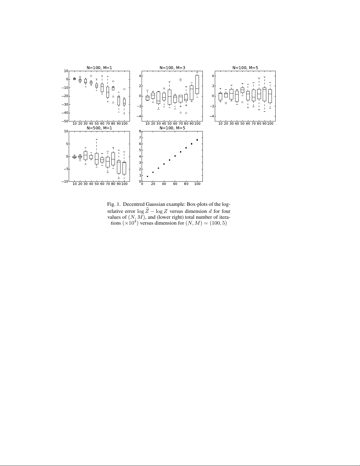
1 2 3 4 5 6 7 8 9 10 11 12 13 14 15 16 17 18 19 20 21 22 23 24 25 26 27 28 29 30 31 32 33 34 35 36 37 38 39 40 41 42 43 44 45 46 47 48 Biometrika (2018), xx , x, pp . 1–16 C  2007 Biometrika T rust Printed in Gr eat Britain Pr operties of nested sampling B Y N I C O L A S C H O P I N CREST –ENSAE, T imbre J120, 3, A venue Pierr e Lar ousse, 92245 Malakoff cede x, F rance nicolas.chopin@ensae.fr A N D C H R I S T I A N P . R O B E RT CEREMADE, Universit ´ e P aris Dauphine, F-75775 P aris cede x 16, F rance xian@ceremade.dauphine.fr S U M M A RY Nested sampling is a simulation method for approximating marginal likelihoods proposed by Skilling (2006). W e establish that nested sampling has an approximation error that v anishes at the standard Monte Carlo rate and that this error is asymptotically Gaussian. W e show that the asymptotic variance of the nested sampling approximation typically gro ws linearly with the dimension of the parameter . W e discuss the applicability and efficiency of nested sampling in realistic problems, and we compare it with two current methods for computing marginal likelihood. W e propose an extension that a voids resorting to Markov chain Monte Carlo to obtain the simulated points. Some ke y wor ds : Central limit theorem; Evidence; Importance sampling; Marginal likelihood; Marko v chain Monte Carlo; Nested sampling. 1. I N T R O D U C T I O N Nested sampling was introduced by Skilling (2006) as a numerical approximation method for integrals of the kind Z = Z L ( y | θ ) π ( θ ) d θ , when π is the prior distribution and L ( y | θ ) is the likelihood. Those integrals are called evidence in the abov e papers. They naturally occur as marginals in Bayesian testing and model choice (Jeffre ys, 1939; Robert, 2001, Chapters 5 and 7). Nested sampling has been well receiv ed in astronomy and has been applied successfully to sev eral cosmological problems, see, for instance, Mukherjee et al. (2006), Sha w et al. (2007), and V egetti & K oopmans (2009), among others. In addition, Murray et al. (2006) dev elop a nested sampling algorithm for computing the normalising constant of Potts models. The purpose of this paper is to in v estigate the formal properties of nested sampling. A first effort in that direction is Evans (2007), which shows that nested sampling estimates con ver ge in probability , b ut calls for further work on the rate of con v er gence and the limiting distribution. Our main result is a central limit theorem for nested sampling estimates, which says that the approx- imation error is dominated by a O ( N − 1 / 2 ) stochastic term, which has a limiting Gaussian distribution, and where N is a tuning parameter proportional to the computational ef fort. W e also in vestigate the im- pact of the dimension d of the problem on the performances of the algorithm. In a simple example, we show that the asymptotic v ariance of nested sampling estimates grows linearly with d ; this means that the computational cost is O ( d 3 /η 2 ) , where η is the selected error bound. One important aspect of nested sampling is that it resorts to simulating points θ i from the prior π , con- strained to θ i having a larger likelihood value than some threshold l . In many cases, the simulated points must be generated by Marko v chain Monte Carlo sampling. W e propose an extension of nested sam- 49 50 51 52 53 54 55 56 57 58 59 60 61 62 63 64 65 66 67 68 69 70 71 72 73 74 75 76 77 78 79 80 81 82 83 84 85 86 87 88 89 90 91 92 93 94 95 96 2 pling, based on importance sampling, that introduces enough flexibility so as to perform the constrained simulation without resorting to Markov chain Monte Carlo. Finally , we examine two alternati ves to nested sampling for computing e vidence, both based on the output of Marko v chain Monte Carlo algorithms. W e do not aim at an exhausti ve comparison with all existing methods, see, for instance, Chen et al. (2000), for a broader revie w , and restrict our attention to methods that share the property with nested sampling that the same algorithm pro vides approximations of both the posterior distribution and the marginal likelihood, at no extra cost. W e provide numerical comparisons between those methods, since some of the aforementioned papers and Murray’ s PhD thesis (2007, Uni versity Colle ge London), also include numerical comparisons of nested sampling with other methods for sev eral models. 2. N E S T E D S A M P L I N G : A D E S C R I P T I O N 2 · 1 . Principle W e briefly describe the nested sampling algorithm, as introduced by Skilling (2006). W e use L ( θ ) as a short-hand for the likelihood L ( y | θ ) , omitting the dependence on y . Nested sampling is based on the following identity: Z = Z 1 0 ϕ ( x ) d x , (1) where ϕ is the in verse of the survi val function of the random v ariable L ( θ ) , ϕ − 1 : l → pr { L ( θ ) > l } , assuming θ ∼ π and ϕ − 1 is a decreasing function, which is the case when L is a continuous function and π has a connected support. The representation Z = E π { L ( θ ) } holds with no restriction on either L or π . Formally , this one-dimensional integral could be approximated by standard quadrature methods, b Z = j X i =1 ( x i − 1 − x i ) ϕ i , (2) where ϕ i = ϕ ( x i ) , and 0 < x j < · · · < x 1 < x 0 = 1 is an arbitrary grid over [0 , 1] . Function ϕ is in- tractable in most cases howe ver , so the ϕ i ’ s are approximated by an iterativ e random mechanism: – Iteration 1: dra w independently N points θ 1 ,i from the prior π , determine θ 1 = arg min 1 ≤ i ≤ N L ( θ 1 ,i ) , and set ϕ 1 = L ( θ 1 ) . – Iteration 2: obtain the N current values θ 2 ,i , by reproducing the θ 1 ,i ’ s, except for θ 1 that is re- placed by a draw from the prior distrib ution π conditional upon L ( θ ) ≥ ϕ 1 ; then select θ 2 as θ 2 = arg min 1 ≤ i ≤ N L ( θ 2 ,i ) , and set ϕ 2 = L ( θ 2 ) . – Iterate the above step until a gi ven stopping rule is satisfied, for instance when observing very small changes in the approximation b Z or when reaching the maximal v alue of L ( θ ) when it is kno wn. In the above, the v alues x ? i = ϕ − 1 ( ϕ i ) that should be used in the quadrature approximation (2) are unknown, b ut they hav e the following property: t i = ϕ − 1 ( ϕ i +1 ) /ϕ − 1 ( ϕ i ) = x ? i +1 /x ? i are independent beta ( N , 1) v ariates. Skilling (2006) proposes two approaches: first, a deterministic scheme, where x i is substituted with exp( − i/ N ) in (2), so that log x i is the expectation of log ϕ − 1 ( ϕ i ) ; second, a random scheme, where K parallel streams of random numbers x i,k , k = 1 , . . . , K , are generated from the same generating process as the x ? i , x i +1 ,k = x i,k t i,k , where t i,k ∼ beta ( N , 1) . In the latter case, a natural esti- mator is: log e Z = 1 K K X k =1 log e Z k , e Z k = j X i =1 ( x i − 1 ,k − x i,k ) ϕ i . 97 98 99 100 101 102 103 104 105 106 107 108 109 110 111 112 113 114 115 116 117 118 119 120 121 122 123 124 125 126 127 128 129 130 131 132 133 134 135 136 137 138 139 140 141 142 143 144 3 For the sake of brevity , we focus on the deterministic scheme in this paper, and study the estimator (2) and x i = exp( − i/ N ) . Furthermore, for K = 1 , the random scheme produces more noisy estimates than the deterministic scheme, but, for large v alues of K , it may be the opposite, see for instance Fig. 3 in Murray et al. (2006). 2 · 2 . V ariations and posterior simulation Skilling (2006) indicates that nested sampling pro vides simulations from the posterior distrib ution at no extra cost: “the existing sequence of points θ 1 , θ 2 , θ 3 , . . . already giv es a set of posterior representativ es, provided the i ’th is assigned the appropriate importance weight ω i L i ”, where the weight ω i is equal to the difference ( x i − 1 − x i ) and L i is equal to ϕ i . This can be justified as follows. Consider the computation of the posterior expectation of a gi ven function f µ ( f ) = Z π ( θ ) L ( θ ) f ( θ ) d θ  Z π ( θ ) L ( θ ) d θ . One can then use a single run of nested sampling to obtain estimates of both the numerator and the denominator , the latter being the evidence Z , estimated by (2). The estimator j X i =1 ( x i − 1 − x i ) ϕ i f ( θ i ) (3) of the numerator is a noisy version of j X i =1 ( x i − 1 − x i ) ϕ i e f ( ϕ i ) , where e f ( l ) = E π { f ( θ ) | L ( θ ) = l } , the prior e xpectation of f ( θ ) conditional on L ( θ ) = l . This Riemann sum is, following the principle of nested sampling, an estimator of the e vidence. L E M M A 1 . Let e f ( l ) = E π { f ( θ ) | L ( θ ) = l } for l > 0 , then, if e f is absolutely continuous, Z 1 0 ϕ ( x ) e f { ϕ ( x ) } d x = Z π ( θ ) L ( θ ) f ( θ ) d θ . (4) A proof is provided in Appendix 1. Clearly , the estimate of µ ( f ) obtained by dividing (3) by (2) is the estimate obtained by computing the weighted av erage mentioned above. W e do not discuss further this aspect of nested sampling, but our con vergence results can be e xtended to such estimates. 3. A C E N T R A L L I M I T T H E O R E M F O R N E S T E D S A M P L I N G W e decompose the approximation error of nested sampling as follows: j X i =1 ( x i − 1 − x i ) ϕ i − Z 1 0 ϕ ( x ) d x = − Z ε 0 ϕ ( x ) d x + ( j X i =1 ( x i − 1 − x i ) ϕ ( x i ) − Z 1 ε ϕ ( x ) d x ) + j X i =1 ( x i − 1 − x i ) { ϕ i − ϕ ( x i ) } . The first term is a truncation error, resulting from the feature that the algorithm is run for a finite time. For simplicity’ s sake, we assume that the algorithm is stopped at iteration j = d ( − log ε ) N e , where d x e stands for the smallest integer k such that x ≤ k , so that x j = exp( − j / N ) ≤ ε < x j − 1 . More practi- cal stopping rules are discussed in § 7. Assuming ϕ , or equiv alently L , bounded from above, the error R ε 0 ϕ ( x ) d x is exponentially small with respect to the computational effort. The second term is a numerical integration error , which, provided ϕ 0 is bounded over [ ε, 1] , is of order O ( N − 1 ) , since x i − 1 − x i = O ( N − 1 ) . 145 146 147 148 149 150 151 152 153 154 155 156 157 158 159 160 161 162 163 164 165 166 167 168 169 170 171 172 173 174 175 176 177 178 179 180 181 182 183 184 185 186 187 188 189 190 191 192 4 The third term is stochastic and is denoted η N = j X i =1 ( x i − 1 − x i ) { ϕ ( x ? i ) − ϕ ( x i ) } , where the x ? i ’ s are such that ϕ i = L ( θ i ) = ϕ ( x ? i ) , therefore x ? i = ϕ − 1 ( ϕ i ) . The following theorem characterises the asymptotic beha viour of η N . T H E O R E M 1 . Pr ovided that ϕ is twice continuously-differ entiable over [ ε, 1] , and that its two first derivatives ar e bounded over [ ε, 1] , then N 1 / 2 η N con verg es in distribution to a Gaussian distrib ution with mean zer o and variance V = − Z s,t ∈ [ ε, 1] sϕ 0 ( s ) tϕ 0 ( t ) log( s ∨ t ) d s d t. The stochastic error is of order O P ( N − 1 / 2 ) and it dominates both other error terms. The proof of this theorem relies on the functional central limit theorem and is detailed in Appendix 2. A straightforward application of the delta-method sho ws that the log-scale error , log b Z − log Z , has the same asymptotic behaviour , but with asymptotic variance V / Z 2 . 4. P R O P E RT I E S O F T H E N E S T E D S A M P L I N G A L G O R I T H M 4 · 1 . Simulating fr om a constrained prior The main difficulty of nested sampling is to simulate θ from the prior distrib ution π subject to the constraint L ( θ ) > L ( θ i ) ; exact simulation from this distribution is an intractable problem in many realistic set-ups. It is at least of the same complexity as a one-dimensional slice sampler, which produces an uniformly ergodic Markov chain when the likelihood L is bounded but may be slow to conv erge in other settings (Roberts & Rosenthal, 1999). Skilling (2006) proposes to sample v alues of θ by iterating M Markov chain Monte Carlo steps, using the truncated prior as the in variant distrib ution, and a point chosen at random among the N − 1 survi vors as the starting point. Since the starting value is already distributed from the inv ariant distribution, a finite number M of iterations produces an outcome that is marginally distributed from the correct distribution. This howe ver introduces correlations between simulated points. W e stress that our central limit theorem applies no longer when simulated points are not independent, and that the consistency of nested sampling estimates based on Mark ov chain Monte Carlo is an open problem. A reason wh y such a theoretical result seems difficult to establish is that each iteration in volv es both a different Markov chain Monte Carlo kernel and a different in variant distrib ution. There are settings when implementing a Markov chain Monte Carlo mo ve that leaves the truncated prior in variant is not straightforward. In those cases, one may instead implement an Mark ov chain Monte Carlo mov e, for instance a random walk Metropolis–Hastings move, with respect to the unconstrained prior , and subsample only values that satisfy the constraint L ( θ ) > L ( θ i ) , but this scheme gets increasingly inefficient as the constraint mov es closer to the highest v alues of L . More adv anced sampling schemes can be de vised that ov ercome this dif ficulty , such as the use of a diminishing v ariance f actor in the random walk. In § 5, we propose an e xtension of nested sampling based on importance sampling. In some settings, this may facilitate the design of efficient Marko v chain Monte Carlo steps, or ev en allo w for sampling independently the θ i ’ s. 4 · 2 . Impact of dimensionality W e show in this section that the theoretical performance of nested sampling typically depends on the dimension d of the problem as follo ws: the required number of iterations and the asymptotic v ariance both grow linearly with d . Thus, if a single iteration costs O ( d ) , the computational cost of nested sampling is O ( d 3 /η 2 ) , where η denotes a giv en error level; Murray’ s PhD thesis also states this result, using a more 193 194 195 196 197 198 199 200 201 202 203 204 205 206 207 208 209 210 211 212 213 214 215 216 217 218 219 220 221 222 223 224 225 226 227 228 229 230 231 232 233 234 235 236 237 238 239 240 5 heuristic ar gument. This result applies to the exact nested algorithm only . In principle, resorting to Mark ov chain Monte Carlo might entail some additional curse of dimensionality , but this point seems difficult to study formally , and will only be briefly inv estigated in our simulation studies. Consider the case where, for k = 1 , . . . , d , θ ( k ) ∼ N (0 , σ 2 0 ) , and y ( k ) | θ ( k ) ∼ N ( θ ( k ) , σ 2 1 ) , indepen- dently in both cases. Set y ( k ) = 0 and σ 2 0 = σ 2 1 = 1 / 4 π , so that Z = 1 for all d ’ s. A draw from the con- strained prior is obtained as follo ws: simulate r 2 ≤ − 2 1 / 2 log l from a truncated χ 2 ( d ) distrib ution and u 1 , . . . , u d ∼ N (0 , 1) , then set θ ( k ) = r u k / ( u 2 1 + . . . + u 2 d ) 1 / 2 . Since Z = 1 , we assume that the trunca- tion point ε d is such that ϕ (0) ε d = τ  1 , τ = 10 − 6 say , where ϕ (0) = 2 d/ 2 is the maximum likelihood value. Therefore, ε d = τ 2 − d/ 2 and the number of iterations required to produce a given truncation error , that is, j = d ( − log  ) N e , grows linearly in d . T o assess the dependence of the asymptotic variance with respect to d , we state the following lemma, established in Appendix 3. L E M M A 2 . In the current setting, if V d is the asymptotic variance of the nested sampling estima- tor with truncation point ε d , ther e exist constants c 1 , c 2 such that V d /d ≤ c 1 for all d ≥ 1 , and lim inf d → + ∞ V d /d ≥ c 2 . This lemma is easily generalised to cases where the prior is such that the components are independent and identically distributed, and the likelihood factorises as L ( θ ) = Q d k =1 L ( θ ( k ) ) . W e conjecture that V d /d con ver ges to a finite v alue in all these situations and that, for more general models, the variance grows linearly with the actual dimensionality of the problem, as measured for instance in Spiegelhalter et al. (2002). 5. N E S T E D I M P O RTA N C E S A M P L I N G W e introduce an e xtension of nested sampling based on importance sampling. Let e π ( θ ) an instrumental prior with the support of π included in the support of e π , and let e L ( θ ) an instrumental lik elihood, namely a positiv e measurable function. W e define an importance weight function w ( θ ) such that e π ( θ ) e L ( θ ) w ( θ ) = π ( θ ) L ( θ ) . W e can approximate Z by nested sampling for the pair ( e π , e L ) , that is, by simulating iterati vely from e π constrained to e L ( θ ) > l , and by computing the generalised nested sampling estimator j X i =1 ( x i − 1 − x i ) ϕ i w ( θ i ) . (5) The advantage of this e xtension is that one can choose ( e π , e L ) so that simulating from e π under the constraint e L ( θ ) > l is easier than simulating from π under the constraint L ( θ ) > l . For instance, one may choose an instrumental prior e π such that Markov chain Monte Carlo steps adapted to the instrumental constrained prior are easier to implement than with respect to the actual constrained prior .In a similar vein, nested importance sampling facilitates contemplating sev eral priors at once, as one may compute the evidence for each prior by producing the same nested sequence, based on the same pair ( e π , e L ) , and by simply modifying the weight function. Ultimately , one may choose ( e π , e L ) so that the constrained simulation is performed exactly . F or instance, if e π is a Gaussian N d ( ˆ θ , ˆ Σ) distrib ution with arbitrary hyper -parameters, take e L ( θ ) = λ n ( θ − ˆ θ ) T ˆ Σ − 1 ( θ − ˆ θ ) o , where λ is an arbitrary decreasing function. Then ϕ i w ( θ i ) = e L ( θ i ) w ( θ i ) = π ( θ i ) L ( θ i )  e π ( θ i ) . In this case, the x i ’ s in (2) are error-free: at iteration i , θ i is sampled uniformly ov er the ellipsoid that con- tains exactly exp( − i/ N ) prior mass as θ i = q i C v / k v k 1 / 2 2 , where C is the Cholesky lower triangle of ˆ Σ , v ∼ N d (0 , I d ) , and q i is the exp( − i/ N ) quantile of a χ 2 ( d ) distribution. Mukherjee et al. (2006) consider a nested sampling algorithm where simulated points are generated within an ellipsoid, and accepted if they 241 242 243 244 245 246 247 248 249 250 251 252 253 254 255 256 257 258 259 260 261 262 263 264 265 266 267 268 269 270 271 272 273 274 275 276 277 278 279 280 281 282 283 284 285 286 287 288 6 respect the likelihood constraint, b ut their algorithm is not based on the importance sampling extension described here. The nested ellipsoid strategy seems useful in two scenarios. First, assume both the posterior mode and the Hessian at the mode are av ailable numerically and tune ˆ θ and ˆ Σ accordingly . In this case, this strat- egy should outperform standard importance sampling based on the optimal Gaussian proposal, because the nested ellipsoid strategy uses a O ( N − 1 ) quadrature rule on the radial axis, along which the weight function v aries the most; see § 7 · 3 for an illustration. Second, assume only the posterior mode is av ailable, so one may set ˆ θ to the posterior mode, and set ˆ Σ = τ I d , where τ is an arbitrary , large value. Section 7 · 3 indicates that the nested ellipsoid strategy may still perform reasonably in such a scenario. Models such that the Hessian at the mode is tedious to compute include in particular Gaussian state space models with missing observations (Brockwell & Davis, 1996, Chap. 12), Markov modulated Poisson processes (Ryd ´ en, 1994), or , more generally , models where the e xpectation-maximisation algorithm (see MacLach- lan & Krishnan, 1997) is the easiest way to compute the posterior mode, although one may use Louis’ (1982) method for computing the information matrix from the expectation-maximisation output. 6. A LT E R N A T I V E A L G O R I T H M S 6 · 1 . Appr oximating Z fr om a posterior sample As recalled in § 2 · 2, the output of nested sampling can be “recycled” so as to approximate posterior quantities. Con versely , one can recycle the output of an Marko v chain Monte Carlo algorithm towards estimating the evidence, with no or little additional programming effort; see for instance Gelfand & Dey (1994), Meng & W ong (1996), and Chen & Shao (1997). W e describe below the solutions used in the subsequent comparison with nested sampling, but we do not pretend at an e xhaustiv e co verage of those techniques, see Chen et al. (2000) or Han & Carlin (2001) for a deeper coverage, nor at using the most efficient approach, see Meng & Schilling (2002). 6 · 2 . Appr oximating Z by a formal r eversible jump W e first recov er Gelfand and De y’ s (1994) solution of reverse importance sampling by an integrated rev ersible jump, because a natural approach to compute a marginal likelihood is to use a reversible jump Markov chain Monte Carlo algorithm (Green, 1995). Ho wever , this may seem wasteful as it in volv es sim- ulating from sev eral models, while only one is of interest. But we can in theory contemplate a single model M and still implement re versible jump in the follo wing way . Consider a formal alternati ve model M 0 , for instance a fixed distrib ution like the N (0 , 1) distribution, with prior weight 1 / 2 and b uild a proposal from M to M 0 that moves to M 0 with probability (Green, 1995) ρ M→M 0 = { (1 / 2) g ( θ ) }  { (1 / 2) π ( θ ) L ( θ ) } ∧ 1 and from M 0 to M with probability ρ M 0 → M = { (1 / 2) π ( θ ) L ( θ ) }  { (1 / 2) g ( θ ) } ∧ 1 , g ( θ ) being an ar - bitrary proposal on θ . W ere we to actually run this re versible jump Marko v chain Monte Carlo algorithm, the frequency of visits to M would then con verge to Z . Howe ver , the re versible sampler is not needed since, if we run a standard Markov chain Monte Carlo algorithm on θ and compute the probability of moving to M 0 , the expectation of the ratio g ( θ ) /π ( θ ) L ( θ ) is equal to the in verse of Z : E  g ( θ )  π ( θ ) L ( θ )  = Z g ( θ ) π ( θ ) L ( θ ) π ( θ ) L ( θ ) Z d θ = 1  Z , no matter what g ( θ ) is, in the spirit of both Gelf and & Dey (1994) and Bartolucci et al. (2006). Obviously , the choice of g ( θ ) impacts on the precision of the approximated Z . When using a k ernel approximation to π ( θ | y ) based on earlier Markov chain Monte Carlo simulations and considering the variance of the resulting estimator, the constraint is opposite to the one found in importance sampling, namely that g ( θ ) must ha ve lighter (not fatter) tails than π ( θ ) L ( θ ) for the approximation c Z 1 = 1  ( 1 T T X t =1 g ( θ ( t ) ) π ( θ ( t ) ) L ( θ ( t ) ) ) 289 290 291 292 293 294 295 296 297 298 299 300 301 302 303 304 305 306 307 308 309 310 311 312 313 314 315 316 317 318 319 320 321 322 323 324 325 326 327 328 329 330 331 332 333 334 335 336 7 to ha ve a finite v ariance. This means that light tails or finite support kernels, lik e an Epanechnikov kernel, are to be preferred to fatter tails kernels, lik e the t kernel. In the experimental comparison reported in § 7 · 2, we compare c Z 1 with a standard importance sampling approximation c Z 2 = 1 T T X t =1 π ( θ ( t ) ) L ( θ ( t ) )  g ( θ ( t ) ) , θ ( t ) ∼ g ( θ ) , where g can also be a non-parametric approximation of π ( θ | y ) , this time with heavier tails than π ( θ ) L ( θ ) . Fr ¨ uhwirth-Schnatter (2004) uses the same importance function g in both c Z 1 and c Z 2 , and obtain results similar to ours, namely that c Z 2 outperforms c Z 1 . 6 · 3 . Appr oximating Z using a mixtur e repr esentation Another approach in the approximation of Z is to design a specific mixture for simulation purposes, with density proportional to m ( θ ) ∝ ω 1 π ( θ ) L ( θ ) + g ( θ ) where ω 1 > 0 and g ( θ ) is an arbitrary , fully specified density . Simulating from this mixture has the same complexity as simulating from the posterior, the Markov chain Monte Carlo code used to simulate from π ( θ | y ) can be easily extended by introducing an auxiliary v ariable δ that indicates whether or not the current simulation is from π ( θ | y ) or from g ( θ ) . The t -th iteration of this extension is as follows, where K ( θ , θ 0 ) denotes an arbitrary Markov chain Monte Carlo kernel associated with the posterior π ( θ | y ) ∝ π ( θ ) L ( θ ) : 1. T ake δ ( t ) = 1 , and δ ( t ) = 2 otherwise, with probability ω 1 π ( θ ( t − 1) ) L ( θ ( t − 1) )  n ω 1 π ( θ ( t − 1) ) L ( θ ( t − 1) ) + g ( θ ( t − 1) ) o ; 2. If δ ( t ) = 1 , generate θ ( t ) ∼ Markov chain Monte Carlo ( θ ( t − 1) , θ ( t ) ) , else generate θ ( t ) ∼ g ( θ ) inde- pendently from the previous v alue θ ( t − 1) . This algorithm is a Gibbs sampler: Step 1 simulates δ ( t ) conditional on θ ( t − 1) , while Step 2 simulates θ ( t ) conditional on δ ( t ) . While the average of the δ ( t ) ’ s con verges to ω 1 Z/ { ω 1 Z + 1 } , a natural Rao- Blackwellisation is to take the a verage of the e xpectations of the δ ( t ) ’ s, ˆ ξ = 1 T T X t =1 ω 1 π ( θ ( t ) ) L ( θ ( t ) )  n ω 1 π ( θ ( t ) ) L ( θ ( t ) ) + g ( θ ( t ) ) o , since its variance should be smaller . A third estimate is then deduced from this approximation by solving ω 1 ˆ Z 3 / { ω 1 ˆ Z 3 + 1 } = ˆ ξ . The use of mixtures in importance sampling in order to improv e the stability of the estimators dates back at least to Hesterber g (1998) but, as it occurs, this particular mixture estimator happens to be almost identical to the bridge sampling estimator of Meng & W ong (1996). In fact, ˆ Z 3 = 1 ω 1 T X t =1 ω 1 π ( θ ( t ) ) L ( θ ( t ) ) ω 1 π ( θ ( t ) ) L ( θ ( t ) ) + g ( θ ( t ) )  T X t =1 g ( θ ( t ) ) ω 1 π ( θ ( t ) ) L ( θ ( t ) ) + g ( θ ( t ) ) is the Monte Carlo approximation to the ratio E m { α ( θ ) π ( θ ) L ( y | θ ) } /E m [ α ( θ ) g ( θ )] when using the optimal function α ( θ ) = 1  { ω 1 π ( θ ) L ( θ ) + g ( θ ) } . The only dif ference with Meng & W ong (1996) is that, since θ ( t ) ’ s are simulated from the mixture, they can be rec ycled for both sums. 337 338 339 340 341 342 343 344 345 346 347 348 349 350 351 352 353 354 355 356 357 358 359 360 361 362 363 364 365 366 367 368 369 370 371 372 373 374 375 376 377 378 379 380 381 382 383 384 8 10 20 30 40 50 60 70 80 90 100 50 40 30 20 10 0 10 N=100, M=1 10 20 30 40 50 60 70 80 90 100 4 2 0 2 4 N=100, M=3 10 20 30 40 50 60 70 80 90 100 4 2 0 2 4 N=100, M=5 0 20 40 60 80 100 0 1 2 3 4 5 6 7 8 N=100, M=5 10 20 30 40 50 60 70 80 90 100 10 5 0 5 10 N=500, M=1 Fig. 1. Decentred Gaussian example: Box-plots of the log- relativ e error log b Z − log Z versus dimension d for four values of ( N , M ) , and (lo wer right) total number of itera- tions ( × 10 4 ) versus dimension for ( N , M ) = (100 , 5) 7. N U M E R I C A L E X P E R I M E N T S 7 · 1 . A decentr ed Gaussian example W e modify the Gaussian toy example presented in § 4 · 2: θ = ( θ (1) , . . . , θ ( d ) ) , where the θ ( k ) ’ s are in- dependent and identically distributed from N (0 , 1) , and y k | θ ( k ) ∼ N ( θ ( k ) , 1) independently , b ut setting all the y k ’ s to 3 . T o simulate from the prior truncated to L ( θ ) > L ( θ 0 ) , we perform M Gibbs iterations with respect to this truncated distribution, with M = 1 , 3 or 5: the full conditional distribution of θ ( k ) , conditional on θ ( j ) , j 6 = k , is a N (0 , 1) distrib ution that is truncated to the interval [ y ( k ) − δ, y ( k ) + δ ] with δ 2 = X j ( y j − θ ( j ) 0 ) 2 − X j 6 = k ( y j − θ ( j ) ) 2 . The nested sampling algorithm is run 20 times for d = 10 , 20 , . . . , 100 , and sev eral combinations of ( N , M ) : (100 , 1) , (100 , 3) , (100 , 5) , and (500 , 1) . The algorithm is stopped when a new contribution ( x i − 1 − x i ) ϕ i to (2) becomes smaller than 10 − 8 times the current estimate. Focussing first on N = 100 , Fig. 1 exposes the impact of the mixing properties of the Markov chain Monte Carlo step: for M = 1 , the bias sharply increases with respect to the dimension, while, for M = 3 , it remains small for most dimensions. Results for M = 3 and M = 5 are quite similar , except perhaps for d = 100 . Using M = 3 Gibbs steps seems to be sufficient to produce a good approximation of an ideal nested sampling algorithm, where points would be independently simulated. Interestingly , if N increases to 500 , while keeping M = 1 , then larger errors occur for the same computational effort. Thus, a good strategy in this case is to increase first M until the distrib ution of the error stabilises, then to increase N to reduce the Monte Carlo error . As expected, the number of iterations linearly increases with the dimension. While artificial, this example shows that nested sampling may perform quite well even in large dimen- sion problems, provided M is large enough. 385 386 387 388 389 390 391 392 393 394 395 396 397 398 399 400 401 402 403 404 405 406 407 408 409 410 411 412 413 414 415 416 417 418 419 420 421 422 423 424 425 426 427 428 429 430 431 432 9 7 · 2 . A mixtur e example As in Fr ¨ uhwirth-Schnatter (2004), we consider the example of the posterior distrib ution on ( µ, σ ) asso- ciated with the normal mixture y 1 , . . . , y n ∼ p N (0 , 1) + (1 − p ) N ( µ, σ ) , (6) when p is known, for tw o compelling reasons. First, when σ con ver ges to 0 and µ is equal to an y of the x i ’ s (1 ≤ i ≤ n ) , the likelihood div erges, see Fig. 2. This is a priori challenging for exploratory schemes such as nested sampling. Second, efficient Marko v chain Monte Carlo strategies have been de veloped for mixture models (Diebolt & Robert, 1994; Richardson & Green, 1997; Celeux et al., 2000), b ut Bayes factors are dif ficult to approximate in this setting. W e simulate n observations from a N (2 , (3 / 2) 2 ) distrib ution, and then compute the estimates of Z introduced above for the model (6). The prior distrib ution is uniform on ( − 2 , 6) × (0 · 001 , 16) for ( µ, log σ 2 ) . The prior is arbitrary , but it allows for an easy implementation of nested sampling since the constrained simulation can be implemented via a random walk mov e. The two-dimensional nature of the parameter space allows for a numerical integration of L ( θ ) , based on a Riemann approximation and a grid of 800 × 500 points in the ( − 2 , 6) × (0 · 001 , 16) square. This approach leads to a stable e valuation of Z that can be taken as the reference against which we can test the various methods, since additional e valuations based on a crude Monte Carlo integration using 10 6 terms and on Chib’ s (1995) produced essentially the same numerical values. The Markov chain Monte Carlo algorithm implemented here is the standard completion of Diebolt & Robert (1994), but it does not suffer from the usual label switching deficiency (Jasra et al., 2005) because (6) is identifiable. As shown by the Markov chain Monte Carlo sample of size N = 10 4 displayed on the left hand side of Fig. 2, the exploration of the modal region by the Markov chain Monte Carlo chain is satisfactory . This Markov chain Monte Carlo sample is used to compute the non-parametric approximations g that appear in the three alternativ es of § 6. For the reverse importance sampling estimate Z 1 , g is a product of two Gaussian kernels with a bandwidth equal to half the default bandwidth of the R function density(), while, for both Z 2 and Z 3 , g is a product of two t kernels with a bandwidth equal to twice the default Gaussian bandwidth. W e ran the nested sampling algorithm, with N = 10 3 , reproducing the implementation of Skilling (2006), namely using 10 steps of a random walk in ( µ, log σ ) constrained by the likelihood boundary . based on the contribution of the current value of ( µ, σ ) to the approximation of Z . The ov erall number of points produced by nested sampling at stopping time is on average close to 10 4 , which justifies using the same number of points for the Markov chain Monte Carlo algorithm. As shown on the right hand side of Fig. 2, the nested sampling sequence visits the minor modes of the likelihood surface b ut it ends up in the same central mode as the Markov chain Monte Carlo sequence. All points visited by nested sampling are represented without reweighting, which explains for a larger density of points outside the central modal region. The analysis of this Monte Carlo experiment in Fig. 3 first sho ws that nested sampling gives approx- imately the same numerical v alue when compared with the three other approaches, exhibiting a slight upward bias, but that its variability is higher . The most reliable approach, besides the numerical and raw Monte Carlo e valuations which cannot be used in general settings, is the importance sampling solution, followed very closely by the mixture approach of § 6 · 3. The re verse importance sampling naturally sho ws a slight upward bias for the smaller values of n and a variability that is very close to both other alternati ves, especially for larger v alues of n . 7 · 3 . A pr obit example for nested importance sampling T o implement the nested importance sampling algorithm based on nested ellipsoids, we consider the arsenic dataset and a probit model studied in Chapter 5 of Gelman & Hill (2006). The observations are independent Bernoulli v ariables y i such that extpr ( y i = 1 | x i ) = Φ( x T i θ ) , where x i is a vector of d cov ariates, θ is a vector parameter of size d , and Φ denotes the standard normal distribution function. In this particular example, d = 7 ; more details on the data and the cov ariates are av ailable on the book’ s web-page ( http://www.stat.columbia.edu/˜gelman/arm/examples/arsenic ). 433 434 435 436 437 438 439 440 441 442 443 444 445 446 447 448 449 450 451 452 453 454 455 456 457 458 459 460 461 462 463 464 465 466 467 468 469 470 471 472 473 474 475 476 477 478 479 480 10 Fig. 2. Mixture example: (left) Marko v chain Monte Carlo sample plotted on the log-likelihood surface in the ( µ, σ ) space for n = 10 observations from (6) (right) nested sam- pling sequence based on N = 10 3 starting points for the same dataset ● ● ● ● ● ● ● ● ● ● ● ● ● ● ● ● ● ● ● ● ● ● ● ● ● ● ● ● ● ● nested reverse importance mixture 0.8 0.9 1.0 1.1 1.2 ● ● ● ● ● ● ● ● ● ● ● ● ● ● ● ● ● ● ● nested reverse importance mixture 0.8 1.0 1.2 1.4 ● ● ● ● ● ● ● ● ● ● ● ● ● nested reverse importance mixture 0.8 1.0 1.2 1.4 Fig. 3. Mixture model: comparison of the variations of nested sampling, re verse importance sampling, importance sampling and mixture sampling, relati ve to a numerical ap- proximation of Z (dotted line), based on 150 samples of size n = 10 , 50 , 100 The probit model we use is model 9a in the R program a vailable at this address: the dependent v ariable indicates whether or not the surveyed individual changed the well she drinks from over the past three years, and the se ven cov ariates are an intercept, distance to the nearest safe well (in 100 metres unit), education lev el, log of arsenic lev el, and cross-effects for these three variables. W e assign N d (0 , 10 2 I d ) as our prior on θ , and denote θ m the posterior mode, and Σ m the inv erse of minus twice the Hessian at the mode; both quantities are obtained numerically beforehand. W e run the nested ellipsoid algorithm 50 times, for N = 2 , 8, 32, 128, and for two sets of hyper- parameters corresponding to both scenarios described in § 5. In the first scenario, ( ˆ θ , ˆ Σ) = ( θ m , 2Σ m ) . The bottom ro w of Fig. 4 compares log-errors produced by our method (left), with those of importance sampling based on the optimal Gaussian proposal, with mean θ m , variance Σ m , and the same number of likelihood e valuations, as reported on the x-axis of the right plot. In the second scenario, ( ˆ θ , ˆ Σ) = ( θ m , 100 I d ) . The top row of Fig. 4 compares log-errors produced by our method (left) with those of importance sampling, based again on the optimal proposal, and the same number of likelihood ev aluations. The v ariance of importance sampling estimates based on a Gaussian proposal with hyper-parameters ˆ θ and ˆ Σ = 100 I d is higher by sev eral order of magnitudes, and is not reported in the plots. 481 482 483 484 485 486 487 488 489 490 491 492 493 494 495 496 497 498 499 500 501 502 503 504 505 506 507 508 509 510 511 512 513 514 515 516 517 518 519 520 521 522 523 524 525 526 527 528 11 As expected, the first strategy outperforms standard importance sampling, when both methods are sup- plied with the same information (mode, Hessian), and the second strate gy still does reasonably well com- pared to importance sampling based on the optimal Gaussian proposal, although only provided with the mode. Results are sufficiently precise that one can afford to compute the evidence for the 2 7 possible models: the most likely model, with posterior probability 0 . 81 , includes the intercept, the three variables mentioned abo ve, distance, arsenic, education, and one cross-ef fect between distance and education lev el, and the second most likely model, with posterior probability 0 . 18 , is the same model but without the cross-effect. 2 8 32 128 2 1 0 1 2 97 370 1429 5530 2 1 0 1 2 2 8 32 128 2 1 0 1 2 62 244 971 3880 2 1 0 1 2 Fig. 4. Probit example: Box-plots of (left column) log- errors of nested importance sampling estimates, for N = 2 , 8 , 32 , 128 , compared with the log-error of importance sampling estimates (right column) based on the optimal Gaussian proposal, and the same number of likelihood ev aluations. Those are reported on the x axis of the right column plots. The bottom row corresponds to the first strat- egy , based on both mode and Hessian, while the top row corresponds to the second strategy , based on mode only . 8. D I S C U S S I O N Nested sampling is thus a valid addition to the Monte Carlo toolbox, with con vergence rate O ( N − 1 / 2 ) , and computational cost O ( d 3 ) , where d is the dimension of the problem. which enjoys good performances in some applications, for example when the posterior is approximately Gaussian, but which may require more iterations to achieve the same precision in certain situations. Therefore, further work on the formal and practical assessments of nested sampling conv ergence would be welcome. For one thing, the con- ver gence properties of Markov chain Monte Carlo-based nested sampling are unknown and technically challenging. Methodologically , efforts are required to design efficient Markov chain Monte Carlo mov es with respect to the constrained prior . In that and other respects, nested importance sampling may con- 529 530 531 532 533 534 535 536 537 538 539 540 541 542 543 544 545 546 547 548 549 550 551 552 553 554 555 556 557 558 559 560 561 562 563 564 565 566 567 568 569 570 571 572 573 574 575 576 12 stitute a useful e xtension. Ultimately , our comparison between nested sampling and alternati ves should be extended to more diverse examples, in order to get a clearer idea of when nested sampling should be the method of choice and when it should not. For instance, Murray et al. (2006) reports that nested sam- pling strongly outperforms annealed importance sampling (Neal, 2001) for Potts models. All the programs implemented for this paper are av ailable from the authors. A C K N O W L E D G E M E N T The authors are grateful to R. Denny , A. Doucet, T . Loredo, O. Papaspiliopoulos, G. Roberts, J. Skilling, the Editor , the Associate Editor and the referees for helpful comments. The second author is also a mem- ber of the Center for Research in Economy and Statistics (CREST), whose support he gratefully ackno wl- edges. R E F E R E N C E S B A RT O L U C C I , F . , S C A C C I A , L . & M I R A , A . (2006). Efficient Bayes f actor estimation from the reversible jump output. Biometrika 93 , 41–52. B R O C K W E L L , P . & D A V I S , P . (1996). Intr oduction to T ime Series and F orecasting . Springer T exts in Statistics. Springer-V erlag, Ne w Y ork. C E L E U X , G . , H U R N , M . & R O B E RT , C . (2000). Computational and inferential difficulties with mixtures posterior distribution. J. Am. Statist. Assoc. 95(3) , 957–979. C H E N , M . & S H AO , Q . (1997). On Monte Carlo methods for estimating ratios of normalizing constants. Ann. Statist. 25 , 1563–1594. C H E N , M . , S H A O , Q . & I B R A H I M , J . (2000). Monte Carlo Methods in Bayesian Computation . Springer-V erlag, New Y ork. C H I B , S . (1995). Marginal lik elihood from the Gibbs output. J . Am. Statist. Assoc. 90 , 1313–1321. D I E B O LT , J . & R O B E R T , C . (1994). Estimation of finite mixture distributions by Bayesian sampling. J. R. Statist. Soc. A 56 , 363–375. E V A N S , M . (2007). Discussion of nested sampling for Bayesiancomputations by John Skilling. In Bayesian Statistics 8 , J. Bernardo, M. Bayarri, J. Berger , A. David, D. Heckerman, A. Smith & M. W est, eds. Oxford Uni versity Press, pp. 491–524. F R ¨ U H W I RT H - S C H NAT T E R , S . (2004). Estimating mar ginal lik elihoods for mixture and Markov switching models using bridge sampling techniques. The Econometrics J ournal 7 , 143–167. G E L FA N D , A . & D E Y , D . (1994). Bayesian model choice: asymptotics and exact calculations. J . R. Statist. Soc. A 56 , 501–514. G E L M A N , A . & H I L L , J . (2006). Data Analysis Using Re gression and Multilevel/Hierar chical Models . Cambridge, UK: Cambridge Univ ersity Press. G R E E N , P . (1995). Re versible jump MCMC computation and Bayesian model determination. Biometrika 82 , 711– 732. H A N , C . & C A R L I N , B . (2001). MCMC methods for computing Bayes factors: a comparati ve re view . J . Am. Statist. Assoc. 96 , 1122–1132. H E S T E R B E R G , T. (1998). W eighted average importance sampling and defensive mixture distrib utions. T echnometrics 37 , 185–194. J A S R A , A . , H O L M E S , C . & S T E P H E N S , D . (2005). Marko v Chain Monte Carlo methods and the label switching problem in Bayesian mixture modeling. Statist. Sci. 20 , 50–67. J E FF R E Y S , H . (1939). Theory of Pr obability . Oxford: The Clarendon Press, 1st ed. K A L L E N B E R G , O . (2002). F oundations of Modern Pr obability . Springer-V erlag, New Y ork. L O U I S , T. (1982). Finding the observed information matrix when using the EM algorithm. J . R. Statist. Soc. A 44 , 226–233. M A C L A C H L A N , G . & K R I S H N A N , T. (1997). The EM Algorithm and Extensions . New Y ork: John W iley . M E N G , X . & S C H I L L I N G , S . (2002). W arp bridge sampling. J . Comput. Graph. Statist. 11 , 552–586. M E N G , X . & W O N G , W. (1996). Simulating ratios of normalizing constants via a simple identity: a theoretical exploration. Statist. Sinica 6 , 831–860. M U K H E R J E E , P . , P A R K I N S O N , D . & L I D D L E , A . (2006). A Nested Sampling Algorithm for Cosmological Model Selection. The Astr ophysical Journal 638 , L51–L54. M U R R AY , I . , M AC K A Y , D . J . , G H A H R A M A N I , Z . & S K I L L I N G , J . (2006). Nested sampling for Potts models. In Advances in Neural Information Processing Systems 18 , Y . W eiss, B. Sch ¨ olkopf & J. Platt, eds. Cambridge, MA: MIT Press. 577 578 579 580 581 582 583 584 585 586 587 588 589 590 591 592 593 594 595 596 597 598 599 600 601 602 603 604 605 606 607 608 609 610 611 612 613 614 615 616 617 618 619 620 621 622 623 624 13 N E A L , R . (2001). Annealed importance sampling. Stat. Comput. 11 , 125–139. R I C H A R D S O N , S . & G R E E N , P . (1997). On Bayesian analysis of mixtures with an unknown number of components (with discussion). J . R. Statist. Soc. A 59 , 731–792. R O B E RT , C . (2001). The Bayesian Choice . Springer-V erlag, Ne w Y ork, 2nd ed. R O B E RT S , G . & R O S E N T H A L , J . (1999). Con vergence of slice sampler Marko v chains. J. R. Statist. Soc. A 61 , 643–660. R Y D ´ E N , T. (1994). Parameter estimation for Markov modulated Poisson processes. Stochastic Models 10 , 795–829. S H AW , J ., B R I D G E S , M . & H O B S O N , M . (2007). Ef ficient Bayesian inference for multimodal problems in cosmol- ogy . Monthly Not. R. Astrono. Soc. 378 , 1365–1370. S K I L L I N G , J . (2006). Nested sampling for general Bayesian computation. Bayesian Analysis 1(4) , 833–860. S P I E G E L H A LT E R , D . J . , B E S T , N . G . , C A R L I N , B . P . & V A N D E R L I N D E , A . (2002). Bayesian measures of model complexity and fit (with discussion). J . R. Statist. Soc. A 64 , 583–639. V E G E T T I , S . & K O O P M A N S , L . V . E . (2009). Bayesian strong gravitational-lens modelling on adaptiv e grids: objectiv e detection of mass substructure in galaxies. Monthly Not. R. Astr ono. Soc. 392 , 945–963. A P P E N D I X 1 Pr oof of Lemma 1 It is suf ficient to prove this result for functions e f that are real-valued, positi ve and increasing. First, the extension to vector -v alued functions is trivial, so e f is assumed to be real-valued from now on. Second, the class of functions that satisfy property (4) is clearly stable through addition. Since e f is absolutely continuous, there e xist functions f + and f − , such that f + is increasing, f − is decreasing, and e f = f + + f − , so we can restrict our attention to increasing functions. Third, absolute continuity implies bounded variation, so it al ways possible to add an arbitrary constant to e f to transform it into a positi ve function. Let ψ : l → l e f ( l ) , which is a positive, increasing function and denote its in verse by ψ − 1 . One has: E π [ ψ { L ( θ ) } ] = Z + ∞ 0 pr[ ψ { L ( θ ) } > l ] d l = Z + ∞ 0 ϕ − 1 { ψ − 1 ( l ) } d l = Z 1 0 ψ { ϕ ( x ) } d x , which concludes the proof. A P P E N D I X 2 Pr oof of Theor em 1 Let t i = x ? i +1 /x ? i , for i = 0 , 1 , . . . As mentioned by Skilling (2006), the t i ’ s are independent beta ( N , 1) variates. Thus, u i = t N i defines a sequence of independent uniform [0 , 1] v ariates. A T aylor expansion of η N giv es: η N = d cN e X i =1 ( x i − 1 − x i ) { ϕ ( x ? i ) − ϕ ( x i ) } = d cN e X i =1 ( x i − 1 − x i ) n ψ 0 ( − log x i ) (log x i − log x ? i ) + O (log x i − log x ? i ) 2 o where c = − log ε , and ψ ( y ) = ϕ ( e − y ) . Furthermore, S i = N (log x i − log x ? i ) = i − 1 X k =0 ( − 1 − log u k ) 625 626 627 628 629 630 631 632 633 634 635 636 637 638 639 640 641 642 643 644 645 646 647 648 649 650 651 652 653 654 655 656 657 658 659 660 661 662 663 664 665 666 667 668 669 670 671 672 14 is a sum of independent, standard v ariables, as E (log u i ) = − 1 and v ar (log u i ) = 1 . Thus, (log x i − log x ? i ) = O P ( N − 1 / 2 ) , where the implicit constant in O P ( N − 1 / 2 ) does not depend on i , and N 1 / 2 η N = N − 1 / 2 d cN e X i =1 ( e − ( i − 1) / N − e − i/ N ) S i  ψ 0 ( i N ) + O P ( N − 1 / 2 )  = c 1 / 2 d cN e X i =1 Z i/ N ( i − 1) / N e − t ψ 0 ( t ) B N ( t c ) d t n 1 + O P ( N − 1 / 2 ) o , since ψ 0 ( t ) = ψ 0 ( i/ N ) + O ( N − 1 ) for t ∈ [( i − 1) / N , i/ N ] , where, again, the implicit constant in O ( N − 1 ) can be the same for all i , as ψ 00 is bounded, and pro vided B N ( t ) is defined as B N ( t ) = ( cN ) − 1 / 2 S d cN t e for t ∈ [0 , 1] . According to Donsk er’ s theorem (Kallenberg, 2002, p.275), B N con verges to a Bro wnian motion B on [0 , 1] , in the sense that f ( B N ) con verges in distribution to f ( B ) for any measurable and a.s. continuous function f . Thus N 1 / 2 η N = c 1 / 2 Z d cN e /N 0 e − t ψ 0 ( t ) B N ( t c ) d t + O P ( N − 1 / 2 ) con verges in distrib ution to c 1 / 2 Z c 0 e − t ψ 0 ( t ) B ( t c ) d t , which has the same distribution as the follo wing zero-mean Gaussian variate: Z c 0 e − t ψ 0 ( t ) B ( t ) d t = Z 1 ε sϕ 0 ( s ) B ( − log s ) d s. A P P E N D I X 3 Pr oof of Lemma 2 For the sake of clarity , we mak e dependencies on d explicit in this section, including ϕ d for ϕ , ε d for ε , and so on. W e will use repeatedly the facts that ϕ is nonincreasing and that ϕ 0 is nonnegati ve. One has: − Z s,t ∈ [ ε d , 1] sϕ 0 d ( s ) tϕ 0 d ( t ) log( s ∨ t ) d t ≤ − log ε d  Z 1 ε d sϕ 0 d ( s ) d s  2 ≤ d log(2 1 / 2 /τ ) for d ≥ 1 , since − R 1 ε d sϕ 0 d ( s ) d s ≤ − R 1 0 sϕ 0 d ( s ) d s = 1 . This giv es the first result. Let s d = ϕ − 1 d ( α d ) , for 0 < α < 1 ; s d is the probability that (4 π /d ) d X i =1 θ 2 i − 1 ≤ − 2 log( α ) + log(2) − 1 assuming that the θ i ’ s are independent N (0 , 1 / 4 π ) variates. The left-hand side is an empirical a verage of independent and identically distributed zero-mean v ariables. W e tak e α so that the right-hand side is negati ve, which implies α > 2 1 / 2 exp( − 1 / 2) . Using lar ge de viations (Kallenberg, 2002, Chapter 27), one 673 674 675 676 677 678 679 680 681 682 683 684 685 686 687 688 689 690 691 692 693 694 695 696 697 698 699 700 701 702 703 704 705 706 707 708 709 710 711 712 713 714 715 716 717 718 719 720 15 has − log( s d ) /d → γ > 0 as d → + ∞ , and 1 d V d = − 1 d Z s,t ∈ [ ε d , 1] sϕ 0 d ( s ) tϕ 0 d ( t ) log( s ∨ t ) d s d t ≥  − log s d d   Z s d ε d sϕ 0 d ( s ) d s  2 ≥  − log s d d   Z s d ε d ϕ d ( s ) d s + ε d ϕ d ( ε d ) − s d ϕ d ( s d )  2 ≥  − log s d d   1 − Z ε d 0 ϕ d ( s ) d s − Z 1 s d ϕ d ( s ) d s + ε d ϕ d ( ε d ) − s d ϕ d ( s d )  2 . As d → + ∞ , − log( s d ) /d → γ , s d → 0 , ϕ d ( s d ) = α d → 0 , R 1 s d ϕ d ( s ) d s ≤ ϕ d ( s d )(1 − s d ) → 0 , and 0 ≤ Z ε d 0 ϕ d ( s ) d s − ε d ϕ d ( ε d ) ≤ ε d { ϕ d (0) − ϕ d ( ε d ) } ≤ τ < 1 , by the definition of ε d , and the squared factor is in the limit greater than or equal to (1 − τ ) 2 .