On some difficulties with a posterior probability approximation technique

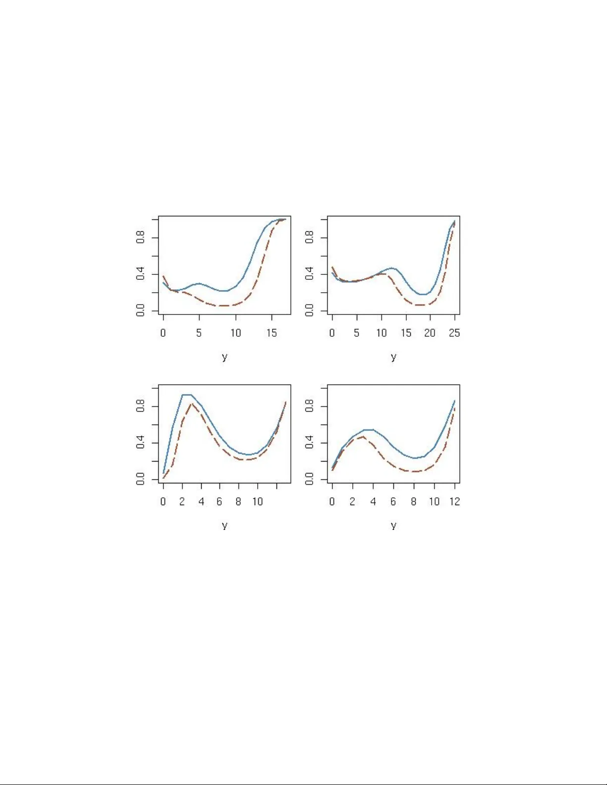
On some difficulties with a p osterio r p robabilit y app ro ximation technique Christian P . Rob ert 1 CEREMADE, Univ ersit ´ e P aris Dauphine, and CREST, INSEE Jean-Mic hel Marin 2 INRIA Sacla y , Univ ersit ´ e P aris Sud, Orsa y , and CREST, INSEE Abstract. In Scott (2002) and Congdon (2006), a new metho d is adv anced to compute p osterior probabilities of mo dels under consideration. It is based solely on MCMC outputs restricted to single mo dels, i.e., it is b ypassing reversible jump and other model exploration tec hniques. While it is indeed possible to appro xi- mate p osterior probabilities based solely on MCMC outputs from single mo dels, as demonstrated b y Gelfand and Dey (1994) and Bartolucci et al. (2006), we show that the prop osals of Scott (2002) and Congdon (2006) are biased and adv ance sev eral argumen ts tow ards this thesis, the primary one b eing the confusion b e- t ween mo del-based posteriors and joint pseudo-p osteriors. F rom a practical point of view, the bias in Scott’s (2002) approximation app ears to b e m uch more severe than the one in Congdon’s (2006), the latter b eing often of the same magnitude as the posterior probabilit y it approximates, although w e also exhibit an example where the div ergence from the true p osterior probability is extreme. Keyw o rds: Ba yesian mo del c hoice, posterior appro ximation, reversible jump, Mark ov Chain Mon te Carlo (MCMC), pseudo-priors, unbiasedness, improp ert y . 1 Intro duction Mo del selection is a fundamental statistical issue and a clear asset of the Bay esian metho dology but it faces severe computational difficulties b ecause of the requirement to explore simultaneously the parameter spaces of all mo dels under comparison accu- rately enough to provide sufficient appro ximations to the posterior probabilities of all mo dels. When Green (1995) introduced reversible jump techniques, it was perceived b y the communit y as the second MCMC revolution in that it allow ed for a v alid and efficien t exploration of the collection of mo dels and the subsequent literature on the topic exploiting reversible jump MCMC is a testimony to the app eal of this me th o d. Nonetheless, the implemen tation of reversible jump techniques in complex situations ma y face difficulties or at least inefficiencies of its own and, despite some recen t ad- v ances in the devising of the jumps underlying reversible jump MCMC (Bro oks et al., 2003), the care required in the construction of those jumps often acts as a deterrent from its applications. There are practical alternatives to rev ersible jump MCMC when the n um b er of mo dels under consideration is small enough to allow for a complete exploration of those mo dels. Integral appro ximations using imp ortance sampling techniques lik e those found c  2008 International So ciet y for Bay esian Analysis ba0001 2 Difficulties with an approximation tec hnique in Gelfand and Dey (1994), based on a harmonic mean representation of the marginal densities, and in Gelman and Meng (1998), fo cussing on the optimised selection of the importance function, are advocated as p oten tial solutions, see Chen et al. (2000) for a detailed in tro duction. The reassessmen t of those metho ds by Bartolucci et al. (2006) sho wed the connection betw een a virtual reversible jump MCMC and imp ortance sampling (see also Chopin and Rob ert, 2007). In particular, those pap ers demonstrated that the output of MCMC samplers on each single mo del could b e used to pro duce appro ximations of posterior probabili ties of those mo dels, via some imp ortance sampling metho dologies also related to Newton and Raftery (1994). In Scott (2002) and Congdon (2006), a new and straightforw ard metho d is adv anced to compute posterior probabilities of mo dels under scrutin y based solely on MCMC outputs restricted to single mo dels. While this simplicit y is quite appealing for the appro ximation of those probabilities, w e b eliev e that b oth proposals of Scott (2002) and Congdon (2006) are inherently biased and we adv ance in this note several arguments to w ards this thesis. In addition, we notice that, to ov ercome the bias w e thus exhibited, a v alid solution would call for the joint simulation of parameters under all models (using priors or pseudo-priors) and, in this step, the pr imary appeal of the metho ds w ould th us b e lost compared to the one prop osed b y Carlin and Chib (1995), from whic h b oth Scott (2002) and Congdon (2006) are inspired. W e wan t to p oin t out at this stage that the original purp ose of Scott (2002) is to pro vide a surv ey of Bay esian metho ds for the analysis of hidden Marko v mo dels and th us that the approximation w e analyse here is introduced as a side remark within the whole pap er. If we insist here on the bias pro duced by Scott’s (2002) approximation, it is b ecause it generated follow ers, including Congdon (2006), and b ecause b oth approx- imations are based on the same erroneous interpretation of the marginal distribution in Bay esian model c hoice. W e also note that Congdon’s (2006) appro ximation often pro duces v alues that are n umerically of the same magnitude as the true v alue of the p osterior probabilities, with sometimes v ery close proximit y as illustrated in Example 2 of Section 3.4, but also p oten tial severe mishaps as in Example 4 of Section 3.4. 2 The metho ds In a Bay esian framework of mo del comparison (see, e.g., Rob ert, 2001), given D mo dels in comp etition, M k , with densities f k ( y | θ k ), and prior probabilities % k = P ( M = k ) ( k = 1 , . . . , D ), the p osterior probabilities of the models M k conditional on the data y are giv en b y P ( M = k | y ) ∝ % k Z f k ( y | θ k ) π k ( θ k ) d θ k , the prop ortionalit y term b eing given b y the sum of the ab o v e and M denoting the unkno wn mo del index. In the specific setup of hidden Marko v mo dels, the solution of Scott (2002, Section Rob ert, C.P ., and Marin, J.-M. 3 4.1) is to generate, sim ultaneously and indep enden tly , D MCMC chains ( θ ( t ) k ) t , 1 ≤ k ≤ D , with stationary distributions π k ( θ k | y ) and to approximate P ( M = k | y ) by ˜ % k ( y ) ∝ % k T X t =1    f k ( y | θ ( t ) k )  D X j =1 % j f j ( y | θ ( t ) j )    , as rep orted in form ula (21) of Scott (2002), with the indication that (21) a verages the D likelihoo ds corresponding to each θ j o v er the life of the Gibbs sampler (p.347), the latter b eing understo od as indep enden tly sampled D parallel Gibbs samplers (p.347). Adopting a more general p ersp ectiv e, the proposal of Congdon (2006) for an appro x- imation of the P ( M = k | y )’s follows b oth from Scott’s (2002) approximation and from the pseudo-prior construction of Carlin and Chib (1995) that predated reversible jump MCMC b y saturating the parameter space with an artificial sim ulation of all parameters at each iteration. Ho wev er, due to a v ery special (and, w e b eliev e, mistak en) c hoice of pseudo-priors discussed below, Congdon’s (2006, p.349) appro ximation of P ( M = k | y ) ev en tually reduces to the estimator ˆ % k ( y ) ∝ % k T X t =1    f k ( y | θ ( t ) k ) π k ( θ ( t ) k )  D X j =1 % j f j ( y | θ ( t ) j ) π j ( θ ( t ) j )    , where the θ ( t ) k ’s are samples from π k ( θ k | y ) (or appro ximate samples obtained b y an MCMC algorithm). This is a simple and readily implementable formula that attracted other researc hers lik e Chen et al. (2008). Although b oth appro ximations ˜ % k ( y ) and ˆ % k ( y ) clearly differ in their expressions, by the addition of a π k ( θ ( t ) k ) term in Congdon’s (2006) formula, they fundamentally relate to the same notion that parameters from other mo dels can b e ignored when conditioning on the mo del index M . This approach is therefore bypassing the simu ltaneous exploration of sev eral parameter spaces and it restricts the simulation effort to marginal samplers on eac h separate mo del. This feature is very appealing since it cuts most of the complexity from the sc hemes b oth of Carlin and Chib (1995) and of Green (1995). W e ho wev er question the foundations of those approximations as presen ted in b oth Scott (2002) and Congdon (2006) and adv ance b elo w argumen ts that b oth authors are using incompatible v ersions of joint distributions on the collection of parameters that jeopardise the v alidity of the appro ximations. 3 Difficulties The sections b elo w expose the difficulties found with b oth methods, following the ar- gumen ts adv anced in Scott (2002) and Congdon (2006), resp ectiv ely . The fundamental 4 Difficulties with an approximation tec hnique difficult y with b oth approac hes app ears to us to stem from a confusion b et ween the mo del dep enden t simulations and the joint simulations based on a pseudo-prior scheme as in Carlin and Chib (1995). Once this difficulty is resolved, it app ears that the corre- sp onding approximation of P ( M = k | y ) by ˆ P ( M = k | y ) do es require a joint sim ulation of all parameters and thus that the solutions proposed in Scott (2002) and Congdon (2006) are of the same complexity as the prop osal of Carlin and Chib (1995). If single mo dels MCMC chains are to b e used, alternative approac hes describ ed for instance in Chen et al. (2000) and compared in Gamerman and Lop es (2006) can b e implemented. 3.1 Inco rrect ma rginals W e denote by θ = ( θ 1 , . . . , θ D ) the collection of parameters for all mo dels under consid- eration. Both Scott (2002) and Congdon (2006) start from the representation P ( M = k | y ) = Z P ( M = k | y, θ ) π ( θ | y ) d θ to justify the appro ximation ˆ P ( M = k | y ) = T X t =1 P ( M = k | y, θ ( t ) ) /T . This is indeed an un biased estimator of P ( M = k | y ) provided the θ ( t ) ’s are generated from the correct (marginal) p osterior π ( θ | y ) = D X k =1 P ( θ, M = k | y ) (1) ∝ D X k =1 % k f k ( y | θ k ) Y j π j ( θ j ) = D X k =1 % k m k ( y ) π k ( θ k | y ) Y j 6 = k π j ( θ j ) . (2) In both pap ers, the θ ( t ) ’s are instead simulated as indep enden t outputs from the comp o- nen t wise posteriors π k ( θ k | y ) and this divergence jeopardises the theoretical v alidity of the appro ximation. The error in b oth interpretations stems from the fact that, while the θ ( t ) k ’s are (correctly) indep enden t given the mo del index M , this indep endence do es not hold once M is integrated out, whic h is the case for the θ ( t ) k ’s in the ab o ve appro ximation ˆ P ( M = k | y ). 3.2 MCMC versus marginal MCMC When Congdon (2006) defines a Marko v chain ( θ ( t ) ) at the top of page 349, he indicates that the comp onen ts of θ ( t ) are made of indep enden t Mark ov chains ( θ ( t ) k ) simulated Rob ert, C.P ., and Marin, J.-M. 5 with MCMC samplers related to the respective marginal posteriors π k ( θ k | y ), follo wing the approach of Scott (2002). The aggregated chain ( θ ( t ) ) is thus stationary against the pro duct of those marginals, D Y k =1 π k ( θ k | y ) . Ho w ev er, in the deriv ation of Carlin and Chib (1995), the mo del is defined in terms of (1) and the Marko v chain should thus b e constructed against (1), not against the pro duct of the mo del marginals. Ob viously , in the case of Congdon (2006), the fact that the pseudo-joint distribution do es not exist b ecause of the flat prior assumption (see Section 3.3 for a pro of ) preven ts this construction but, in the case the flat prior is replaced with a prop er (pseudo-) prior, the same statement holds: the probabilistic deriv ation of P ( M = k | y ) relies on the pseudo-prior construction and, to b e v alid, it do es require the completion step at the core of Carlin and Chib (1995), where parameters need to b e simulated from the pseudo-priors. Generating from the component-wise p osteriors π k ( θ k | y ) pro duces a bias. Similarly , in Scott (2002), the target of the Marko v chain ( θ ( t ) , M ( t ) ) should b e the distribution P ( θ , M = k | y ) ∝ π k ( θ k ) % k f k ( y | θ k ) Y j 6 = k π j ( θ j ) and the θ ( t ) j ’s should th us b e generated from the prior π j ( θ j ) when M ( t ) 6 = j —or equiv a- len tly from the corresp onding marginal if one do es not condition on M ( t ) , but simulating a Mark ov c hain with stationary distribution (2) is certainly a challenge in man y settings if the laten t v ariable decomp osing the sum is not to b e used. Since, in b oth Scott (2002) and Congdon (2006), the ( θ ( t ) )’s are not simulated against the correct target, the resulting av erages of P ( M = k | y, θ ( t ) ), ˜ % k ( y ) and ˆ % k ( y ), will b oth b e biased, as demonstrated in the examples of Section 3.4. 3.3 Imp rop ert y of the p osterio r When resorting to the construction of pseudo-p osteriors adopted by Carlin and Chib (1995), Congdon (2006) uses a flat prior as pseudo-prior on the parameters that are not in mo del M k . More precisely , the join t prior distribution on ( θ, M ) is given by Congdon’s (2006) form ula (2), P ( θ , M = k ) = π k ( θ k ) % k Y j 6 = k π ( θ j | M = k ) = π k ( θ k ) % k , whic h is indeed equiv alent to assuming a flat prior as pseudo-prior on the parameters θ j that are not in mo del M k . Unfortunately , this simplifying assumption has a dramatic consequence in that the 6 Difficulties with an approximation tec hnique corresp onding joint p osterior distribution of θ is nev er defined (as a probability distri- bution) since π ( θ | y ) = D X k =1 π k ( θ k | y ) P ( M = k | y ) do es not integrate to a finite v alue in any of the θ k ’s (unless their supp ort is compact). While Congdon (2006) states that it is not essential that the priors for P ( θ j 6 = k | M = k ) are improp er (p.348), the truth is that they cannot b e improp er. The fact that the p osterior distribution on the saturated vector θ = ( θ 1 , . . . , θ D ) do es not exist obviously has negative consequences on the subsequent deriv ations, since a p ositiv e recurren t Mark ov c hain with stationary distribution π ( θ | y ) cannot b e con- structed. Similarly , the fact that P ( M = k | y ) = Z P ( θ , M = k | Y ) d θ do es not hold any longer. Note that Scott (2002) does not follow the same track: when defining the pseudo- priors in his form ula (20), he uses the pro duct definition 3 P ( θ , M = k ) = π k ( θ k ) % k Y j 6 = k π j ( θ j ) , whic h means that the true priors could also b e used as pseudo-priors across all mo dels. Ho w ev er, we stress that Scott (2002) do es not refer to the construction of Carlin and Chib (1995) in his prop osal, nor do es he use pseudo-priors in his simulations. 3.4 Illustrations W e no w pro ceed through several toy examples where all p osterior quantities can b e computed in order to ev aluate the bias induced b y b oth approximations and w e observe that, despite its theoretical bias, Congdon’s (2006) can sometimes achiev e a close ap- pro ximation of the posterior probability , but also that, in other settings, it may produce an unreliable ev aluation. Example 1. Consider the case when a mo del M 1 : y | θ ∼ U (0 , θ ) with a prior θ ∼ E xp (1) is opp osed to a mo del M 2 : y | θ ∼ E xp ( θ ) with a prior θ ∼ E xp (1). W e also assume equal prior w eigh ts on b oth mo dels: % 1 = % 2 = 0 . 5. The marginals are then m 1 ( y ) = Z ∞ y θ − 1 e − θ d θ = E 1 ( y ) , 3 The indices on the priors hav e b een added to make notations consistent with the present pap er. Rob ert, C.P ., and Marin, J.-M. 7 where E 1 denotes the exp onen tial integral function tabulated b oth in Mathematica and in the GSL lib ra ry , and m 2 ( y ) = Z ∞ 0 θ e − θ ( y +1) d θ = 1 (1 + y ) 2 . F or instance, when y = 0 . 2, the p osterior probability of M 1 is th us equal to P ( M = 1 | y ) = m 1 ( y ) / { m 1 ( y ) + m 2 ( y ) } = E 1 ( y ) / { E 1 ( y ) + (1 + y ) − 2 } ≈ 0 . 6378 , while, for y = 0 . 9, it is approximately 0 . 4843. This means that, in the former case, the Bay es factor of M 1 against M 2 is B 12 ≈ 1 . 760, while for the latter, it decreases to B 12 ≈ 0 . 939. The p osterior on θ in mo del M 2 is a gamma G a (2 , 1 + y ) distribution and it can thus b e simulated directly . F or model M 1 , the p osterior is prop ortional to θ − 1 exp( − θ ) for θ larger than y and it can b e simulated using a standard accept-reject algorithm based on an exp onen tial E xp (1) prop osal translated by y . Using simulations from the true (marginal) posteriors and the appro ximation of Congdon (2006), the numerical v alue of ˆ % 1 ( y ) based on 10 6 sim ulations is 0 . 7919 when y = 0 . 2 and 0 . 5633 when y = 0 . 9, whic h translates in to Ba yes factors of 3 . 805 and of 1 . 288, resp ectiv ely . F or the appro ximation of Scott (2002), the numerical v alue of ˜ % 1 ( y ) is 0 . 6554 (corresp onding to a Bay es factor of 1 . 898) when y = 0 . 2 and 0 . 6789 when y = 0 . 9 (corresp onding to a Bay es factor of 2 . 11), based on the same simulations. Note that in the case y = 0 . 9, a selection based on either appro ximation of the Bay es factor w ould select the wrong mo del. If w e use instead a correct simulation from the join t posterior (2), which can be ac hiev ed by using a Gibbs scheme with target distribution P ( θ , M = k | y ), we then get a prop er MCMC appro ximation to the p osterior probabilities b y the ˆ P ( M = k | y )’s. F or instance, based on 10 6 sim ulations, the numerical v alue of ˆ P ( M = 1 | y ) when y = 0 . 2 is 0 . 6370, while, for y = 0 . 9, it is 0 . 4843. Note that, due to the impropriet y difficulty exp osed in Section 3.3, the equiv alent correction for Congdon’s (2006) sc heme cannot b e implemented. In Figure 1, the three appro ximations are compared to the exact v alue of P ( M = 1 | y ) for a range of v alues of y . The correct sim ulation pro duces a graph that is indistinguish- able from the true probability , while Congdon’s (2006) approximation sta ys within a reasonable range of the true v alue and Scott’s (2002) appro ximation drifts apart for most v alues of y . J The abov e corresp ondence of what is essentially Carlin and Chib’s (1995) scheme with the true n umerical v alue of the posterior probability is obviously unsurprising in this to y example but more adv anced setups see the appro ximation degenerate, since the simulations from the prior are most often inefficient, especially when the num b er 8 Difficulties with an approximation tec hnique Figure 1: Example 1: Comparison of three approximations of P ( M = 1 | y ) with the true v alue (in blue and full lines): Scott’s (2002) appro ximation (in green and mixed dashes), Congdon’s (2006) approximation (in bro wn and dashes), while the correction of Scott’s (2002) approximation is indistinguishable from the true v alue (based on N = 10 6 sim ulations). of mo dels under comparison is large. This is the reason why Carlin and Chib (1995) in tro duced pseudo-priors that were closer appro ximations to the true p osteriors. The pro ximity of Congdon’s (2006) approximation with the true v alue in Figure 1 sho ws that the metho d could p ossibly b e used as a cheap first-order substitute of the true posterior probabilit y if the bias w as better assessed. First, w e note that when all the component wise p osteriors are close to Dirac point masses at v alues ˆ θ k , Congdon’s (2006) appro ximation is close to the true v alue ˆ % k ( y ) ≈ % k f k ( y | ˆ θ k ) π k ( ˆ θ k )  D X j =1 n % j f j ( y | ˆ θ j ) π j ( ˆ θ j ) o . F urther, the p osterior exp ectation of f k ( y | θ ( t ) k ) π k ( θ ( t ) k ) in v olv es the in tegral of Z f k ( y | θ k ) 2 π k ( θ k ) 2 m k ( y ) d y , th us the bias is lik ely to be small in settings where the product f k ( y | θ ( t ) k ) π k ( θ ( t ) k ) is p eak ed as in large samples, for instance. That the bias can almost completely disappear is exp osed through a second toy example. Rob ert, C.P ., and Marin, J.-M. 9 Example 2. Consider the case when a normal mo del M 1 : y ∼ N ( θ , 1) with a prior θ ∼ N (0 , 1) is opp osed to a normal model M 2 : y ∼ N ( θ , 1) with a prior θ ∼ N (5 , 1). W e again assume equal prior w eigh ts. In that case, the marginals are a v ailable in closed form m 1 ( y ) = 1 √ 4 π exp − y 2 4 and m 2 ( y ) = 1 √ 4 π exp − ( y − 5) 2 4 and the p osterior probability of mo del M 1 is P ( M = 1 | y ) =  1 + exp 5(2 y − 5) 4  − 1 . F or argumentation’s sake, assume that we now pro duce b oth sequences ( θ ( t ) 1 ) and ( θ ( t ) 2 ) from the p osterior distributions N ( y / 2 , 1 / 2) and N (( y + 5) / 2 , 1 / 2), respectively , by using the same sequence of  t ∼ N (0 , 1), i.e. θ ( t ) 1 = y 2 + 1 √ 2  t and θ ( t ) 2 = y + 5 2 + 1 √ 2  t . Using those sequences, w e then obtain that exp − 1 2 ( y − θ ( t ) 1 ) 2 − 1 2 ( θ ( t ) 1 ) 2 exp − 1 2 ( y − θ ( t ) 2 ) 2 − 1 2 ( θ ( t ) 2 − 5) 2 = exp − 1 2 ( y − y 2 − 1 √ 2  t ) 2 − 1 2 ( y 2 + 1 √ 2  t ) 2 exp − 1 2 ( y − y +5 2 − 1 √ 2  t ) 2 − 1 2 ( y +5 2 + 1 √ 2  t − 5) 2 = exp − 1 2 ( y 2 − 1 √ 2  t ) 2 − 1 2 ( y 2 + 1 √ 2  t ) 2 exp − 1 2 ( y − 5 2 − 1 √ 2  t ) 2 − 1 2 ( y − 5 2 + 1 √ 2  t ) 2 = exp − 5 4 (2 y − 5) , indep enden tly of  t , and thus that Congdon’s (2006) appro ximation is truly exact using this device! Figure 2 sho ws the difference due to using t wo indep enden t sequences of 10 4  t ’s [instead of one single sequence] and the severe discrepancy resulting from Scott’s appro ximation. (Note that using an artificial MCMC sampler in this case would only increase the v ariabilit y of the approximations.) J The appro ximation m a y also b e rather crude, as shown in the following example, inspired from an example p osted on P eter Congdon’s web-page in connection with Con- gdon (2007). Example 3. Consider comparing M 1 : y ∼ B ( n, p ) when p ∼ B e (1 , 1) with M 2 : y ∼ B ( n, p ) when p ∼ B e ( m, m ). Once again, the p osterior probability can b e computed in closed form since the Ba y es factor is given b y B 12 = ( n + 1)! y !( n − y )! ( m + y − 1)!( m + n − y − 1)! ( m + n − 1)! ( m − 1)! 2 (2 m − 1)! . 10 Difficulties with an approximation tec hnique Figure 2: Example 2: Comparison of t w o approximations of P ( M = 1 | y ) with the true v alue (in blue and full lines): Scott’s (2002) appro ximation (in green and mixed dashes) and Congdon’s (2006) approximation (in brown and long dashes) (based on N = 10 4 sim ulations). The simulations of p ( t ) 1 from the p osterior B e ( y + 1 , n − y + 1) in mo del M 1 and of p ( t ) 2 from the p osterior B e ( y + m, m + n − y ) in model M 2 are straigh tforward (and ob viously do not require an extra MCMC step). Figure 3 shows the impact of Congdon’s (2006) appro ximation on the ev aluation of the posterior probability for n = 15 and m = 100: the magnitude is the same but, in that case, the numerical v alues are quite different. In the case of three mo dels in comp etition, namely when y ∼ B ( n, p ) and the three priors are p ∼ B e (1 , 1), p ∼ B e ( a, b ) and p ∼ B e ( c, d ), the differences may b e of the same order, as shown in Figure 4, but the discrepancy is nonetheless decreasing with the sample size n . J A t last, the approximation ma y fall v ery far from the mark, as demonstrated in the follo wing example where the appro ximation has an asymptotic b eha viour opposite to the one of the true p osterior probability . Example 4. Consider comparing M 1 : y ∼ N (0 , 1 /ω ) with ω ∼ E xp ( a ) against M 2 : exp( y ) ∼ E xp ( λ ) with λ ∼ E xp ( b ). The corresponding marginals are given in closed form b y m 1 ( y ) = Z ∞ 0 r ω 2 π e − ( y 2 / 2) ω ae − aω d ω = a √ 2 π Γ(3 / 2) ( a + y 2 / 2) 3 / 2 Rob ert, C.P ., and Marin, J.-M. 11 Figure 3: Example 3: Comparison of Congdon’s (2006) (in brown and dashed lines) appro ximation of P ( M = 1 | y ) with the true v alue (in blue and full lines) when n = 15 and m = 510 (based on N = 10 4 sim ulations). and m 2 ( y ) = Z ∞ 0 e y λe − e y λ be − bλ d λ = b e y ( b + e y ) 2 . The asso ciated p osteriors are ω | y ∼ G a (3 / 2 , a + y 2 / 2) and λ | y ∼ G a (2 , b + e y ). Figure 5 shows the comparison of the true p osterior probability of M 1 with the approximation for v arious v alues of ( a, b ) and it indicates a very p oor fit when y go es to + ∞ . It is actually possible to sho w that the approximation alwa ys conv erges to 0 when y go es to + ∞ , while the true p osterior probabilit y go es to 1. Indeed, when y go es to + ∞ , the Ba y es factor is m 1 ( y ) m 2 ( y ) ≈ a Γ(3 / 2) b √ 2 π e 2 y e y ( y 2 / 2) 3 / 2 , whic h goes to + ∞ while, since ω ( t ) =  t / ( a + y 2 / 2) and λ ( t ) = υ t / ( b + e y ), with  t ∼ G (3 / 2 , 1) and υ t ∼ G (2 , 1), f 1 ( y | ω ( t ) ) π 1 ( ω ( t ) ) f 2 ( y | λ ( t ) ) π 2 ( λ ( t ) ) = a b √ 2 π √  t e −  t υ t e − υ t b + e y e y ( a + y 2 / 2) 1 / 2 ≈ a b √ 2 π √  t e −  t υ t e − υ t √ 2 y , whic h go es to 0 for all (  t , υ t ). The discrepancy is then extreme. J 12 Difficulties with an approximation tec hnique Figure 4: Example 3: Comparison of Congdon’s (2006) (in brown and dashed lines) approximation of P ( M = 1 | y ) with the true v alue (in blue and full lines) when ( n, a, b, c, d ) is equal to (17 , 2 . 5 , 12 . 5 , 501 . 5 , 500), (25 , 1 . 5 , 4 , 540 , 200), (13 , . 5 , 100 . 5 , 20 , 10) and (12 , . 3 , 1 . 8 , 200 , 200), resp ectiv ely (based on N = 10 4 sim u- lations). Rob ert, C.P ., and Marin, J.-M. 13 Figure 5: Example 4: Comparison of Congdon’s (2006) (in brown and dashed lines) appro ximation of P ( M = 1 | y ) with the true v alue (in blue and full lines) when ( a, b ) is equal to ( . 24 , 8 . 9), ( . 56 , . 7), (4 . 1 , . 46) and ( . 98 , . 081), resp ectiv ely (based on N = 10 4 sim ulations). 14 Difficulties with an approximation tec hnique Ackno wledgements Both authors are grateful to Brad Carlin and to the editorial b oard for helpful sug- gestions and to An tonietta Mira for pro viding a p erfect setting for this w ork during the ISBA-IMS “MCMC’ski 2” conference in Bormio, Italy . The second author is also grateful to Kerrie Mengersen for her invitation to “Spring Bay es 2007” in Co olangatta, Australia, that started our reassessmen t of those papers. This w ork had been supp orted b y the Agence Nationale de la Rec herc he (ANR, 212, rue de Bercy 75012 P aris) through the 2005-2008 pro ject Adap’MC . 4 References Bartolucci, F., L. Scaccia, and A. Mira. 2006. Efficient Bay es factor estimation from the rev ersible jump output. Biometrik a 93: 41–52. Bro oks, S., P . Giudici, and G. Rob erts. 2003. Efficien t construction of reversible jump Mark o v chain Monte Carlo prop osal distributions (with discussion). J. Ro y al Statist. So ciet y Series B 65(1): 3–55. Carlin, B. and S. Chib. 1995. Ba y esian mo del c hoice through Marko v chain Monte Carlo. J. Roy al Statist. So ciet y Series B 57(3): 473–484. Chen, C., R. Gerlach, and M. So. 2008. Bay esian Model Selection for Heteroskedastic Mo dels. Adv ances in Econometrics 23. T o app ear. Chen, M., Q. Shao, and J. Ibrahim. 2000. Monte Carlo Metho ds in Ba yesian Compu- tation . Springer-V erlag, New Y ork. Chopin, N. and C. Rob ert. 2007. Con templating Evidence: prop erties, extensions of, and alternativ es to Nested Sampling. T ech. Rep. 2007-46, CEREMADE, Univ ersit´ e P aris Dauphine. Congdon, P . 2006. Ba y esian mo del choice based on Monte Carlo estimates of p osterior mo del probabilities. Comput. Stat. Data Analysis 50: 346–357. —. 2007. Mo del weigh ts for mo del choice and av eraging. Statistical Metho dology 4(2): 143–157. Gamerman, D. and H. Lop es. 2006. Marko v Chain Mon te Carlo . 2nd ed. Chapman and Hall, New Y ork. Gelfand, A. and D. Dey . 1994. Ba yesian mo del choice: asymptotics and exact calcula- tions. J. Roy al Statist. So ciet y Series B 56: 501–514. Gelman, A. and X. Meng. 1998. Simulating normalizing constants: F rom importance sampling to bridge sampling to path sampling. Statist. Science 13: 163–185. Green, P . 1995. Rev ersible jump MCMC computation and Ba yesian mo del determina- tion. Biometrik a 82(4): 711–732. Rob ert, C.P ., and Marin, J.-M. 15 Newton, M. and A. Raftery . 1994. Approximate Ba yesian inference b y the w eighted lik eliho od b oostrap (with discussion). J. Roy al Statist. So ciet y Series B 56: 1–48. Rob ert, C. 2001. The Bay esian Choice . 2nd ed. Springer-V erlag, New Y ork. Scott, S. L. 2002. Ba y esian metho ds for hidden Mark ov mo dels: recursive computing in the 21st Cen tury . J. American Statist. Asso c. 97: 337–351.