BART: Bayesian additive regression trees

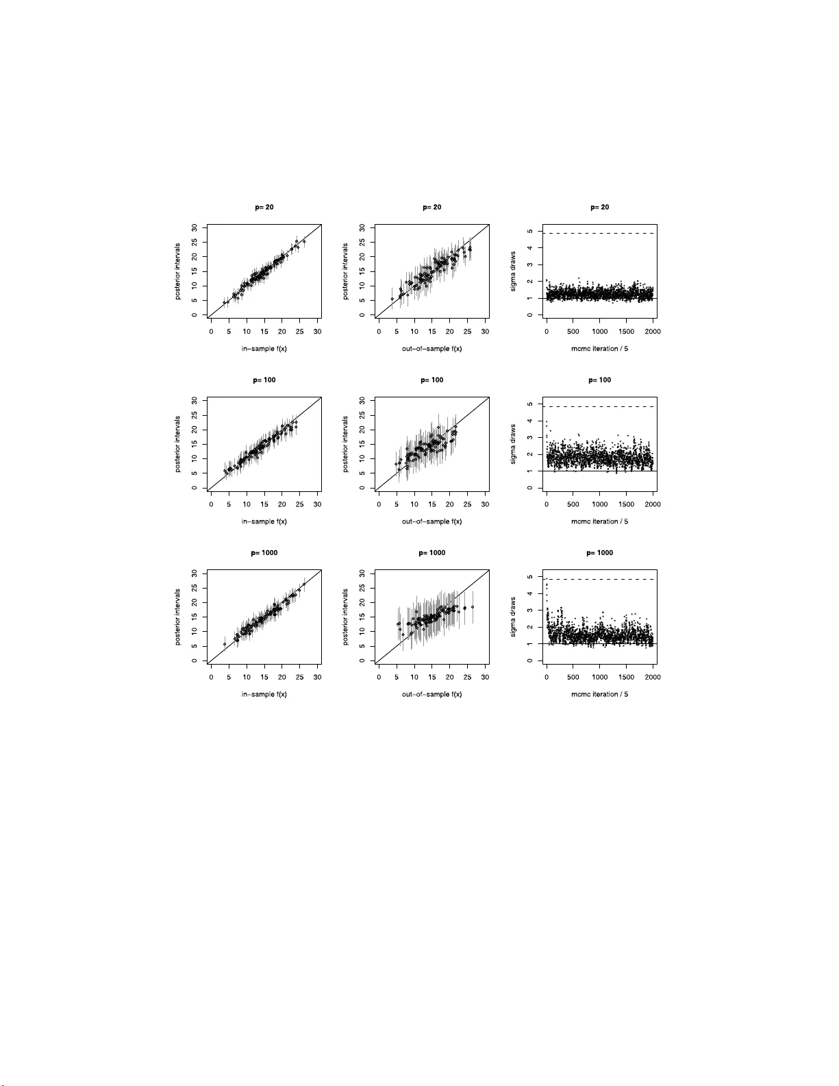
The Annals of Applie d Statistics 2010, V ol. 4, No. 1, 266–298 DOI: 10.1214 /09-A OAS285 c  Institute of Mathematical Statistics , 2 010 BAR T: BA YESIAN ADDITIVE REGRESSION TREES 1 , 2 By Hugh A. Chipman, Edw ard I. Geor ge an d R ob er t E. McCulloch A c adia University, University of Pennsylvania and University of T exas at Austin W e dev elop a Ba yesian “sum-of-trees” mo del where each tree is constrained by a regularization prior to b e a weak learner, and ﬁtting and inference are accomplished v ia an iterative Ba yesian bac k ﬁtting MCMC algorithm that generates samples from a p osterior. Eﬀec- tively , BAR T is a nonparametric Ba yesian regression approac h whic h uses dimensionally adaptiv e random basis elements. Motiv ated b y ensem ble method s in general, and b o osting algorithms in particular, BAR T is deﬁned by a statistical mo del: a prior and a likeli hoo d. T his approac h enables full posterior inference i ncluding p oint and interv al estimates of the unknown regression function as w ell as the marginal eﬀects of p otential pred ictors. By keeping track of p redictor inclusion frequencies, BAR T can also be used for mo del-free va riable selection. BAR T’s many fea tures are illustrated with a bak e-oﬀ ag ainst comp et- ing metho ds on 42 diﬀerent data sets, with a simulation exp eriment and on a drug d isco very classiﬁcation problem. 1. In tro d uction. W e consider the fu ndamenta l problem of making inf er- ence ab out an unknown function f that predicts an output Y using a p dimensional v ector of inputs x = ( x 1 , . . . , x p ) w hen Y = f ( x ) + ε, ε ∼ N (0 , σ 2 ) . (1) T o do this, we consider mo deling or at least app r o ximating f ( x ) = E ( Y | x ), the mean of Y giv en x , by a sum of m r egression trees f ( x ) ≈ h ( x ) ≡ Received June 2008; revised July 2009. 1 Preliminary versi ons of this paper were disseminated as June 2006 and June 2008 technical rep orts. 2 Supp orted by NSF Gran t DMS-06-05102, NSER C and th e Isaac Newton I nstitute for Mathematical Sciences. Key wor ds and phr ases. Ba yes ian bac k ﬁtting, b o osting, CAR T, classiﬁcation, ensem- ble, MCMC, nonparametric regression, probit mo del, rand om basis, regularizatio, sum-of- trees model, va riable selecti on, we ak learner. This is an ele c tr onic re print of the or iginal article published b y the Institute of Mathematical Statistics in The Annals of Applie d S tatistics , 2010, V ol. 4, No. 1, 266– 2 98 . This repr int diﬀers from the origina l in pag ination and typogr aphic detail. 1 2 H. A. CHIPMAN, E. I. GE ORGE AND R. E. MCCULLOCH P m j =1 g j ( x ) where ea c h g j denotes a regression tree. Thus, we approxima te ( 1 ) by a su m-of-trees mo del Y = h ( x ) + ε, ε ∼ N (0 , σ 2 ) . (2) A su m-of-trees mo d el is f undamental ly an additiv e mo del with multiv ari- ate comp onen ts. Compared to generalized additiv e mo dels based on su ms of lo w dimensional smoothers, these multiv ariate comp onen ts can more natu- rally incorp orate in teraction eﬀects. And compared to a single tree mo del, the sum-of-trees can more easily incorp o rate add itiv e eﬀects. V arious metho ds which com bine a set of tree mo dels, so called ensem- ble metho ds, ha ve att racted muc h atten tion. Th ese includ e b o osting [F re- und and Sc hapir e ( 1997 ), F riedman ( 20 01 )], bagging [Breiman ( 1996 )] and random forests [Breiman ( 2001 )], eac h of whic h use diﬀeren t tec hn iques to ﬁt a linear c om bin ation of trees. Boosting ﬁts a sequence of single t rees, using eac h tree to ﬁt data v ariation not explained b y earlie r trees in the sequence. Bagging and random f orests us e r andomization to create a large n u m b er of indep endent trees, and then red uce pred iction v ariance by a ver- aging predictions across the trees. Y e t an other approac h that results in a linear com bination of trees is Ba y esian mo del av eraging applied to the p os- terior arising from a Ba y esian single-tree mo del as in Chipm an , George and McCullo c h ( 1998 ) (hereafte r CGM98) , Denison, Mallic k and S mith ( 1998 ), Blanc hard ( 2004 ) and W u, Tjelmeland and W est ( 2007 ). Suc h mo del a v er- aging us es p osterio r p robabilities as w eigh ts for av eraging the predictions from in dividual tr ees. In this pap er we p r op ose a Ba yesia n a pproac h cal led BAR T (Ba y esian Ad- ditiv e Regression T rees) whic h uses a sum of trees to m o del or appro ximate f ( x ) = E ( Y | x ) . The essen tial idea is to elab orate the sum-of-trees mo del ( 2 ) b y imp osin g a pr ior that regularizes the ﬁt b y k eeping the in dividual tree eﬀects small. In eﬀect, the g j ’s b ecome a dimensionally adaptiv e random basis of “w eak learners,” to b orr o w a ph rase from the b o ost ing literature. By wea k ening the g j eﬀects, BAR T end s up with a sum of trees, ea c h of whic h explains a small and d iﬀerent p ortion of f . Note that BAR T is not equiv alen t to p oste rior a verag ing of single tree ﬁts of the entire function f . T o ﬁt the sum-of-trees mod el, BAR T uses a tailored v ersion of Ba y esian bac kﬁtting MCMC [Hastie and T ibshirani ( 2000 )] that iterativ ely constructs and ﬁts successiv e residuals. Although similar in spirit to the gradien t b o ost- ing appr oac h of F riedman ( 2001 ), BAR T d iﬀers in b ot h ho w it w eak ens the individual trees by instead using a p rior, and ho w it p erf orms the iterativ e ﬁtting by instead usin g Ba y esian backﬁtti ng on a ﬁ xed n um b er of tr ees. Con- ceptually , BAR T can b e view ed as a Bay esian nonparametric approac h that ﬁts a p arameter rich mo del usin g a str on gly in ﬂ uent ial pr ior distrib ution. BAR T 3 Inferences ob tained from BAR T are b ased on successiv e iterations of the bac kﬁtting algorithm wh ic h are eﬀectiv ely an MCMC sample from the in - duced p oste rior ov er th e sum -of-trees mo d el space. A single p osterior mean estimate of f ( x ) = E ( Y | x ) at any inp ut v alue x is obtained by a simple a v- erage of these successiv e sum-of-trees mo d el dra w s ev aluated at x . F urther, p oint wise u ncertain ty in terv als for f ( x ) are easily obtained from th e corre- sp ond in g quan tiles of the sample of dr aws. P oint and interv al estimates are similarly obtained for fun ctionals of f , suc h as p artial dep end ence functions whic h revea l the marginal eﬀects of the x comp onents. Finally , by k eeping trac k of the relativ e frequen cy with whic h x comp o nen ts app ear in the sum- of-trees mo d el iterations, BAR T can b e used to identify whic h comp onents are more imp ortant for explaining the v ariation of Y . S uc h v ariable selec- tion in formation is mo del-free in the sense that it is not based on the usual assumption of an encompassing p arametric mo del. T o facilitate the use of the BAR T metho d s describ ed in this pap er, we ha ve pro v id ed op en-source s oftw are implemen ting BAR T as a stand -alone p ack age or with an in terface to R, along with full d o cumen tation and examples. It is a v ailable as the BayesT ree library in R at http://c ran.r- project.or g/ . The remainder of th e pap er is organized as follo ws . In Section 2 the BAR T mo del is outlined. This consists of the sum-of-trees mo del combined with a regularization prior. In Section 3 a Ba y esian bac kﬁtting MCMC algorithm and metho d s for inference are describ ed. In Section 4 w e describ e a pr obit extension of BAR T for cla ssiﬁcation of binary Y . In Section 5 examples, b oth sim ulated and real, are used to demons tr ate the p oten tial of BAR T. Section 6 p r o vides stu dies of execution time. Section 7 d escrib es extensions and a v ariet y of recent dev elopmen ts and applications of BAR T based on an early version of this pap er. Section 8 concludes with a discussion. 2. The BAR T mo del. As describ ed in the In tro duction , the BAR T mo del consists of t w o p arts: a sum-of-trees mo del a nd a regularization prior on the parameters of that m o del. W e describ e eac h of these in detail in th e follo w in g subsections. 2.1. A sum-of-tr e es mo del. T o ela b orate the f orm of th e sum-of-trees mo del ( 2 ), w e b egin b y establishing notati on for a single tree mo d el. Let T d en ote a binary t ree consisting of a set of in terior no de decision rules and a set o f terminal no d es, and let M = { µ 1 , µ 2 , . . . , µ b } denote a set of parameter v alues asso ci ated with eac h of the b terminal no d es of T . The decision rules are binary sp lits of the predictor space of the form { x ∈ A } vs { x / ∈ A } wh ere A is a subset of the range of x . T hese are typica lly b ased on th e s ingle comp onen ts of x = ( x 1 , . . . , x p ) and are of the form { x i ≤ c } v s { x i > c } f or con tinuous x i . Each x v alue is asso ciated with a single terminal no de of T b y the sequence of decision ru les fr om top to b ottom, and is then 4 H. A. CHIPMAN, E. I. GE ORGE AND R. E. MCCULLOCH assigned the µ i v alue asso ci ated with this terminal no d e. F or a giv en T and M , w e u se g ( x ; T , M ) to denote the function w h ic h assigns a µ i ∈ M to x . Th us, Y = g ( x ; T , M ) + ε, ε ∼ N (0 , σ 2 ) (3) is a sin gle tree mo del of th e form co n sidered b y CGM98. Under ( 3 ), the conditional mean of Y giv en x , E ( Y | x ) equals the terminal no de parameter µ i assigned b y g ( x ; T , M ) . With this notation, the su m-of-trees mo d el ( 2 ) can b e more exp licitly expressed as Y = m X j =1 g ( x ; T j , M j ) + ε, ε ∼ N (0 , σ 2 ) , (4) where for eac h binary regression tree T j and its asso ciated term in al no d e parameters M j , g ( x ; T j , M j ) is the function whic h assigns µ ij ∈ M j to x . Under ( 4 ), E ( Y | x ) e quals the sum of all the terminal no de µ ij ’s assigned to x by the g ( x ; T j , M j )’s. When the n u m b er of trees m > 1, eac h µ ij here is merely a p art of E ( Y | x ), unlik e th e single tree mo del ( 3 ). F ur th ermore, eac h suc h µ ij will represent a main eﬀe ct when g ( x ; T j , M j ) dep ends on only one comp onen t of x (i.e., a single v ariable), and will represen t an inte rac- tion eﬀect wh en g ( x ; T j , M j ) dep ends on more than one comp onen t of x (i.e., more than one v ariable). Thus, t he sum-of-trees mo del can incorp orate b oth main eﬀects and in teraction eﬀects. And b ecause ( 4 ) ma y b e based on trees of v arying sizes, the interacti on eﬀe cts ma y b e of v arying ord ers. In the sp ecia l case wh ere ev ery terminal no de assignment dep end s on just a single comp onent of x , the sum-of-trees mo d el r educes to a simple additive function, a su m of step fun ctions of the individual comp onents of x . With a large num b er of trees, a sum-of-trees mo del gains increased rep- resen tation ﬂ exibilit y whic h, as we’ll see, endows BAR T w ith excellen t pre- dictiv e capabilities. Th is representa tional ﬂexibilit y is obtained b y rapidly increasing the num b er of parameters. Indeed, for ﬁxed m , eac h s u m-of-trees mo del ( 4 ) is determined by ( T 1 , M 1 ) , . . . , ( T m , M m ) a nd σ , whic h includ es all the b ot tom n o de parameters as well as the tree structures and deci- sion rules. F ur ther, the represen tational ﬂexibilit y of eac h individual tree leads to sub stan tial redund ancy ac ross the tr ee comp onent s. Ind eed, one can reg ard { g ( x ; T 1 , M 1 ) , . . . , g ( x ; T m , M m ) } as an “o v ercomplete basis” in the sense that m an y diﬀeren t c hoices of ( T 1 , M 1 ) , . . . , ( T m , M m ) can lead to an iden tical f u nction P m j =1 g ( x ; T j , M j ). 2.2. A r e gularization prior. W e complete the BAR T mo del sp eciﬁcation b y imp osing a prior ov er all the parameters of the sum -of-trees mo d el, namely , ( T 1 , M 1 ) , . . . , ( T m , M m ) and σ . As discussed b elo w, we adv o cate BAR T 5 sp eciﬁcations of this pr ior that eﬀect iv ely regularize the ﬁt by kee ping the individual tree eﬀects from b ei ng unduly inﬂuent ial. Without suc h a regu- larizing in ﬂuence, la rge tree comp onents w ould o verwhelm the ric h structur e of ( 4 ), thereb y limiting the adv antag es of the additiv e represen tation b oth in terms of function app ro ximation and computation. T o facil itate the easy implemen tation of BAR T in practice, w e recom- mend automatic default sp eciﬁcatio n s b elo w whic h app ea r t o b e remark ably eﬀectiv e, as demonstrated in th e many examples of Section 5 . Basically w e pro ceed b y ﬁrst red ucing the prior f ormulation problem to the sp eci ﬁcation of j ust a few interpretable hyp erparameters wh ich go vern p riors on T j , M j and σ . Our r ecommended d efaults are then obtained by using the obs er ved v ariation in y to gauge reasonable hyp erparameter v alues wh en external sub jectiv e in formation is u na v ailable. Alternativ ely , one can u se the consid - erations b elo w to sp ecify a range of p lausible h yp er p arameter v alues and then u se cross-v alidation to select from these v alues. This will of course b e computationally more demanding. W e should also men tion that although we sacriﬁce Ba y esian coherence b y using the data to calibrate our priors, our o ve rriding conce rn is to m ak e s u re th at our pr iors are not in sev ere conﬂ ict with the d ata. 2.2.1. Prior indep endenc e and symmetry. Sp ec iﬁcation of our regular- ization p rior is v astly simp liﬁ ed by r estricting atten tion to pr iors for which p (( T 1 , M 1 ) , . . . , ( T m , M m ) , σ ) =  Y j p ( T j , M j )  p ( σ ) (5) =  Y j p ( M j | T j ) p ( T j )  p ( σ ) and p ( M j | T j ) = Y i p ( µ ij | T j ) , (6) where µ ij ∈ M j . Under suc h priors, th e tree comp onent s ( T j , M j ) are inde- p endent of eac h other and of σ , an d the terminal no d e parameters of ev ery tree are ind ep endent. The indep endence restrict ions ab o ve simplify th e prior sp eciﬁcation prob- lem to the sp eciﬁcation of forms for ju s t p ( T j ) , p ( µ ij | T j ) and p ( σ ) , a sp eci- ﬁcation wh ic h w e fur th er s im p lify by using ident ical forms for all p ( T j ) an d for all p ( µ ij | T j ). As describ ed in the ensuing sub sections, for these w e u se the same prior forms pr op osed by C GM98 for Ba ye sian CAR T. In addition to their v aluable computational b eneﬁts, these forms are co n tr olled b y just a few in terp r etable hyp er p arameters which can b e calibrated using the data 6 H. A. CHIPMAN, E. I. GE ORGE AND R. E. MCCULLOCH to yield eﬀectiv e d efault sp eciﬁcations for r egularizatio n of the sum-of-trees mo del. Ho wev er, as will b e se en, consid er ations for t he choice of these hyp er - parameter v alues for BAR T are markedly diﬀeren t than those for Ba yesian CAR T. 2.2.2. The T j prior. F or p ( T j ), th e form recommended b y CGM98 is easy to sp ecify and d o vet ails nicely w ith calculatio n s for the bac k ﬁ tting MCMC algorithm describ ed later in S ection 3.1 . It is sp eciﬁed by three asp ec ts: (i) the probability that a no de at d epth d (= 0 , 1 , 2 , . . . ) is nonterminal, giv en b y α (1 + d ) − β , α ∈ (0 , 1) , β ∈ [0 , ∞ ) , (7) (ii) the distrib u tion on the sp litting v ariable assignmen ts at eac h in terior no de, and (iii) the distribution on the splitting rule assignmen t in eac h in- terior no d e, conditional on the splitting v ariable. F or (ii) and (iii) w e use the simple defaults used b y CGM98, namely , the un if orm prior on a v ail- able v ariables for (ii) and th e uniform prior on th e discrete set of a v ailable splitting v alues for (iii). Although n ot strictly coheren t from the Ba y esian p oint of view, this last c hoice has the app ea l of in v ariance u nder mon otone transformations of the sp litting v ariables. In a single tree mo del (i.e., m = 1), a tree with man y terminal no des may b e needed to mo del a complicated structure. Ho w ever, for a sum-of-trees mo del, esp ecially with m large, we w an t the regularization p rior to kee p th e individual tree comp onen ts small. In our examples in Section 5 , we do so b y using α = 0 . 95 and β = 2 in ( 7 ). With this c hoice, trees with 1, 2, 3, 4 and ≥ 5 terminal no des receiv e prior probabilit y of 0.05, 0.5 5, 0.28 , 0.09 and 0.03, resp ectiv ely . Note th at ev en with this pr ior, wh ic h puts most p robabilit y on tree sizes of 2 or 3, trees with man y terminal no des can b e gro wn if the data demands it. F or example, in one of our sim u lated examples with this prior, w e observed consid erable p osterior probabilit y on trees of size 17 wh en w e set m = 1 . 2.2.3. The µ ij | T j prior. F or p ( µ ij | T j ), we u s e the conjugate norm al dis- tribution N ( µ µ , σ 2 µ ) wh ic h oﬀers tremendous computational b eneﬁts b e- cause µ ij can b e margined out. T o guide the sp eciﬁcation of the h yp er- parameters µ µ and σ µ , note that E ( Y | x ) is the sum of m µ ij ’s und er the sum-of-trees mo del, and b ecause the µ ij ’s are apriori i.i.d., the in - duced prior on E ( Y | x ) is N ( mµ µ , mσ 2 µ ). Note also that it is highly probable that E ( Y | x ) is b et w een y min and y max , the observ ed minimum and maxi- m u m of Y in the data. Th e essence o f our strategy is then to c h o ose µ µ and σ µ so that N ( mµ µ , mσ 2 µ ) assigns sub stan tial p robabilit y to the int erv al ( y min , y max ). This can b e con v eniently done by c ho osing µ µ and σ µ so that mµ µ − k √ mσ µ = y min and mµ µ + k √ mσ µ = y max for some pr eselected v alue BAR T 7 of k . F or example, k = 2 w ou ld yield a 95% p rior pr obabilit y that E ( Y | x ) is in the interv al ( y min , y max ). The strategy ab ov e uses an asp ect of the observ ed d ata, namely , y min and y max , to try to ensu re that the implicit pr ior for E ( Y | x ) is in the r igh t “ballpark.” That is to sa y , w e w an t it to assign substan tial probabilit y to the en tire region of plausible v alues of E ( Y | x ) while a voiding o v erconcen tration and o verdisp ersion. W e hav e found that, as long as this goal is met, BAR T is v ery robust to c hanges in the exact sp eciﬁca tion. S uc h a data-informed prior appr oac h is esp eci ally u s eful in our pr oblem, wh ere reliable sub jectiv e information ab out E ( Y | x ) is likely to b e unav ailable. F or conv enience, we implement our sp eciﬁcation strategy by ﬁrst s hifting and rescaling Y so that t he ob s erv ed transformed y v alues range from y min = − 0 . 5 to y max = 0 . 5, and then treating this transformed Y as our dep end en t v ariable. W e th en simply cen ter the pr ior for µ ij at zero µ µ = 0 and c h o ose σ µ so th at k √ mσ µ = 0 . 5 for a suitable v alue of k , yielding µ ij ∼ N (0 , σ 2 µ ) where σ µ = 0 . 5 /k √ m. (8) This prior has the eﬀect of s h rinking the tree parameters µ ij to wa rd zero, limiting the eﬀect of the individual tree comp onents of ( 4 ) by k eeping them small. Note that as k and/or th e n umb er of tr ees m is increased, th is prior will b ecome tigh ter and apply greater shrink age to th e µ ij ’s. Prior shrink age on the µ ij ’s is the coun terpart of the shrin k age p arameter in F riedman’s ( 2001 ) gradient b o osting algorithm. T he prior standard deviation σ µ of µ ij here and th e gradient b oosting shr ink age parameter there b oth serve to “w eak en” the ind ividual trees so that eac h is constrained to play a smaller role in the o verall ﬁt. F or the c hoice of k , w e ha ve f ound th at v alues of k b et w een 1 and 3 yield goo d resu lts, an d we recommend k = 2 as an automatic default choic e. Alternative ly , the v alue of k ma y b e c hosen by cross-v alidation from a r an ge of reasonable c hoices. Although the calibratio n of this prior is based on a simp le linear tr ans- formation of Y , it should b e noted that there is no n eed to transf orm the predictor v ariables. This is a consequence of th e f act that th e tr ee sp litting rules are inv arian t to m onotone transformations of the x comp onen ts. The simplicit y of our prior for µ ij is an app ea lin g feature of BAR T. In cont rast, metho ds lik e neural nets that use linear com b inations of predictors require standardization c h oices for eac h predictor. 2.2.4. The σ prior. F or p ( σ ) , we a lso use a conju gate prior, here the in verse c h i-square d istribution σ 2 ∼ ν λ/χ 2 ν . T o guide the sp eciﬁcation of the h y p erparameters ν and λ , we again us e a d ata-informed prior appr oac h, in this case to assign su bstan tial probability to the entire region of plausib le v alues of σ wh ile a voiding o v erconcen tration and o v erd isp ersion. Essent ially , 8 H. A. CHIPMAN, E. I. GE ORGE AND R. E. MCCULLOCH Fig. 1. Thr e e priors on σ b ase d on df = ν and q uantile = q when ˆ σ = 2 . w e calibrate the p rior df ν and scale λ for this purp ose u sing a “rough data- based o veresti mate” ˆ σ of σ . Tw o natural c hoices for ˆ σ are (1) the “naiv e” sp eciﬁcation, in which we tak e ˆ σ to b e the sample standard deviation of Y , or (2) the “linea r mo d el” sp eciﬁcation, in wh ic h w e tak e ˆ σ as th e residual standard deviatio n fr om a least squares linear regression of Y on the original X ’s. W e t hen p ick a v alue of ν b et w een 3 and 10 to g et an ap p ropriate shap e, and a v alue of λ so that the q th quantile of the prior on σ is lo cated at ˆ σ , that is, P ( σ < ˆ σ ) = q . W e consider v alues of q suc h as 0.75, 0.90 or 0.99 to cen ter the distribution b elow ˆ σ . Figure 1 illustrates priors corresp onding to three ( ν, q ) settings wh en the rough ov erestimate is ˆ σ = 2. W e refer to these three settings, ( ν, q ) = (10 , 0 . 75), (3 , 0 . 90), (3 , 0 . 99), as conserv ativ e, d efault and aggressiv e, resp ec- tiv ely . T he prior mo de m ov es to ward smaller σ v alues as q is in creased. W e recommend against c ho osing ν < 3 b ecause it seems to concen trate too m uc h mass on v ery small σ v alues, whic h leads to o verﬁtting. In our examples, we ha ve foun d th ese thr ee settings to w ork very well and yield s im ilar results. F or automatic use, w e recommend th e default sett ing ( ν, q ) = (3 , 0 . 90) whic h tends to a void extremes. Alternativ ely , the v alues of ( ν , q ) m ay b e c hosen by cross-v alidatio n from a r ange of reasonable choi ces. 2.2.5. The choic e of m . A ma j or d iﬀerence betw een BAR T a nd b o osting metho ds is that for a ﬁ x ed num b er of trees m , BAR T u s es an iterativ e bac k - ﬁtting algorithm (describ ed in S ection 3.1 ) to cycle o ve r and o v er through the m trees. If BAR T is to b e u sed for estimating f ( x ) or p redicting Y , it migh t b e reasonable to treat m as an unkno wn paramete r , p utting a pr ior on BAR T 9 m an d pro ceeding with a fu lly Ba yes imp lemen tation of BAR T. Another rea- sonable strategy might b e to select a “b est” v alue for m by cross-v alidation from a range of reasonable c hoices. Ho wev er, b oth of these strategies su b- stan tially increase computational requirements. T o a v oid the computational costs of these strategies, w e ha ve found it fast and exp edien t for estimation an d prediction to b egin w ith a default of m = 200, and then p erhaps to c hec k if one or tw o other c hoices mak es any diﬀerence. Our exp erience has b een that as m is increased, starting with m = 1, the pr edictiv e p erformance of BAR T impro ves dr amatically until at some p oint it level s oﬀ and th en b egins to very slo wly degrade for large v alues of m . Thus, for prediction, it seems only imp ortant to a v oid choosing m to o small. As will b e seen in Section 5 , BAR T yielded excellen t predictive p erformance on a wide v ariet y of examples with the simple default m = 200. Finally , as we shall s ee later in Sections 3.2 and 5 , other considerations for c ho osin g m come in to p la y wh en BAR T is used for v ariable selection. 3. E xtracting information from the p osterior. 3.1. A Bayesian b ackﬁtting MCMC algorithm. Giv en the observed data y , our Ba y esian setup ind uces a p osterior distr ibution p (( T 1 , M 1 ) , . . . , ( T m , M m ) , σ | y ) (9) on all the unkn o wns that d etermine a sum-of-trees mo del ( 4 ). Although the sheer size of the parameter space precludes exhaus tive calc ulation, the follo wing bac kﬁtting MCMC algorithm can b e used to sample from this p osterior. A t a general leve l, our algorithm is a Gibbs samp ler. F or n otational con- v enience, let T ( j ) b e the set of all trees in th e sum exc ept T j , and s im ilarly deﬁne M ( j ) . Thus, T ( j ) will b e a s et of m − 1 trees, and M ( j ) the asso ciated terminal no de parameters. The Gibb s sampler here ent ails m su ccessiv e dra w s of ( T j , M j ) conditionally on ( T ( j ) , M ( j ) , σ ): ( T j , M j ) | T ( j ) , M ( j ) , σ, y , (10) j = 1 , . . . , m , follo w ed b y a draw of σ from the full conditional: σ | T 1 , . . . , T m , M 1 , . . . , M m , y . (11) Hastie and Tibs hirani ( 2000 ) co nsidered a similar application of the Gibbs sampler for p osterior samplin g f or add itiv e an d generalized additive mo dels with σ ﬁxed, and show ed h o w it w as a sto chastic generaliza tion of the bac k- ﬁtting algorithm for suc h mo dels. F or this reason, we refer to our algorithm as b ac kﬁtting MCMC. The d ra w o f σ in ( 11 ) is simply a dr a w from an in verse gamma distribution and s o can b e easily obtained by routine metho ds. More chall enging is h o w 10 H. A. CHIPMAN, E. I. GE ORGE AND R. E. MCCULLOCH to imp lement the m dra ws of ( T j , M j ) in ( 10 ). This can b e done b y taking adv an tage of the follo win g reductions. First, observe th at the conditional distribution p ( T j , M j | T ( j ) , M ( j ) , σ, y ) d ep ends on ( T ( j ) , M ( j ) , y ) only through R j ≡ y − X k 6 = j g ( x ; T k , M k ) , (12) the n -vect or of p artial r esiduals b ased on a ﬁt that excludes the j th tree. Th us, the m d ra ws of ( T j , M j ) giv en ( T ( j ) , M ( j ) , σ, y ) in ( 10 ) are equiv alent to m draws from ( T j , M j ) | R j , σ, (13) j = 1 , . . . , m . No w ( 13 ) is formally equ iv alent to the p osterior of the sin gle tree mo del R j = g ( x ; T j , M j ) + ε w here R j pla ys the role of the data y . Because w e hav e used a conju gate pr ior for M j , p ( T j | R j , σ ) ∝ p ( T j ) Z p ( R j | M j , T j , σ ) p ( M j | T j , σ ) dM j (14) can b e obtained in closed form up to a normin g constant. This allo w s us to carry out eac h dra w fr om ( 13 ) in tw o successiv e steps as T j | R j , σ, (15) M j | T j , R j , σ. (16) The dra w of T j in ( 15 ), although somewh at elab orat e, can b e obtained using the Metrop olis–Hastings (MH) algorithm of CGM98. This algorithm prop oses a new tree based on the current tree u sing one of four mo v es. The mo ves and their asso ciated pr op osal probabilities are as follo ws: gro w ing a terminal no de (0.25), pr uning a pair of termin al no des (0.25), c hanging a n on termin al rule (0.40), and swa p ping a ru le b et w een paren t and c hild (0.10) . Although the gro w a nd p r une mo v es change the num b er of termi- nal no d es, b y integ r ating out M j in ( 14 ), we a vo id the complexities asso ci- ated with rev ersible jump s betw een con tinuous spaces o f v ary in g dimensions [Green ( 1995 )]. Finally , the dr aw of M j in ( 16 ) is simply a set of indep enden t dra ws of the termin al no de µ ij ’s from a normal distribu tion. The d ra w of M j enables the calculation of the subsequ en t residu al R j +1 whic h is critical for the next dra w of T j . F ortunately , there is again n o need for a c omplex rev ersible jump implemen tation. W e initialize the c hain with m simple s in gle no de trees, and then itera- tions are r ep eated until satisfact ory con v ergence is obtained. A t eac h iter- ation, ea c h tree ma y increase or decrease the n um b er of terminal n o des b y one, or c h ange one or tw o decision ru les. Eac h µ will c hange (o r cease to BAR T 11 exist or b e b orn), and σ will change. It is not u ncommon for a tree to grow large and t hen subsequently collapse bac k down to a single no d e as the algo- rithm iterates. The sum-of-trees mo del, with its abundance of uniden tiﬁ ed parameters, all o ws for “ﬁt” to b e freely reallo cated from one tree to another. Because eac h mov e mak es only small incremental c hanges to the ﬁt, we can imagine th e algorithm as analogous to sculp ting a complex ﬁ gure by adding and s u btracting small dabs of cla y . Compared to the single tree mo del MCMC app roac h o f CGM98, our bac k- ﬁtting MCMC algorithm mixes dramatically b etter. When only single tree mo dels are consid ered, the MCMC algorithm tends to q u ic kly gravit ate to- w ard a sin gle large tree and then gets stuc k in a lo cal neighborh o o d of that tree. In sharp con trast, w e ha ve found that restarts of the b ac kﬁtting MCMC algorithm giv e remark ably similar results ev en in diﬃcult pr ob lems. Consequent ly , w e run one l ong chain with BAR T rather t han multiple s tarts. Although m ixing d o es not app ear to b e an issue, the recen tly prop osed mod- iﬁcations of Blanc hard ( 2004 ) and W u, Tjelmeland and W est ( 2007 ) might w ell pro vide additional b eneﬁts. 3.2. Posterior infer enc e statistics. Th e b ac kﬁtting algorithm describ ed in the p revious section is e rgo dic, generating a sequence of dra ws of ( T 1 , M 1 ) , . . . , ( T m , M m ) , σ whic h is con vergi ng (in distribu tion) to the p osterior p (( T 1 , M 1 ) , . . . , ( T m , M m ) , σ | y ). The induced sequence of su m -of-trees fun c- tions f ∗ ( · ) = m X j =1 g ( · ; T ∗ j , M ∗ j ) , (17) for the sequence of d r a ws ( T ∗ 1 , M ∗ 1 ) , . . . , ( T ∗ m , M ∗ m ), is th us con v erging to p ( f | y ), the p osterior distribution on the “true” f ( · ). Thus, by r unnin g the algorithm long enough after a suitable burn -in p eriod, the sequence of f ∗ dra w s, sa y , f ∗ 1 , . . . , f ∗ K , ma y b e regarded as an appr o ximate, d ep endent sam- ple of size K fr om p ( f | y ). Bay esian inferen tial quan tities of in terest c an then b e appro ximated with this sample as indicate d b elo w . Although the n umb er of iterations needed for r eliable inferences w ill of course dep end on the par- ticular app lication, our exp erience with th e examples in S ection 5 suggests that th e num b er of iterations required is relativ ely mo dest. T o estimate f ( x ) or predict Y at a p articular x , in-sample or out-of- sample, a natural choice is th e a v erage of the after burn-in sample f ∗ 1 , . . . , f ∗ K , 1 K K X k =1 f ∗ k ( x ) , (18) whic h app ro ximates the p osterior mean E ( f ( x ) | y ). Another go o d c h oice w ould b e the median of f ∗ 1 ( x ) , . . . , f ∗ K ( x ) whic h appro ximates the p osterior 12 H. A. CHIPMAN, E. I. GE ORGE AND R. E. MCCULLOCH median of f ( x ). P osterior uncertain ty ab out f ( x ) may b e gauged by the v ari- ation of f ∗ 1 ( x ) , . . . , f ∗ K ( x ). F or example, a natural and con venien t (1 − α )% p osterior interv al for f ( x ) is obtained as th e in terv al b et ween the upp er and lo we r α/ 2 qu an tiles of f ∗ 1 ( x ) , . . . , f ∗ K ( x ). As will b e seen, these uncertain ty in terv als b ehav e sensibly , f or example, by widen ing at x v alues far from the data. It is also straigh tforward to use f ∗ 1 ( x ) , . . . , f ∗ K ( x ) to estimate other func- tionals of f . F or example, a fun ctional of particular int erest is the partial dep end ence function [F riedman ( 2001 )], w hic h summarizes the marginal ef- fect of on e (or more) pr edictors on the r esp onse. More pr ecisely , letting f ( x ) = f ( x s , x c ) wh ere x has b een partitioned into the pr edictors of in ter- est, x s and the complement x c = x \ x s , th e p artial dep endence f unction is deﬁned as f ( x s ) = 1 n n X i =1 f ( x s , x ic ) , (19) where x ic is the i th observ ation of x c in the data. Note that ( x s , x ic ) will not generally b e one of the observ ed data p oint s. A dra w fr om the induced BAR T p osterior p ( f ( x s ) | y ) at an y v alue of x s is obtained by simply computing f ∗ k ( x s ) = 1 n P i f ∗ k ( x s , x ic ). Th e a v erage of f ∗ 1 ( x s ) , . . . , f ∗ K ( x s ) then yields an estimate of f ( x s ), and the upp er a n d low er α/ 2 qu an tiles pro vide end p oints of (1 − α )% p osterior interv als for f ( x s ). Finally , as m en tioned in Sectio n 1 , BAR T can also b e u s ed for v ariable selection by select ing those v ariables that app ear most often in the ﬁ tted sum-of-trees mo dels. In terestingly , this strategy is less eﬀectiv e when m is large b ecause the redu ndancy oﬀered b y so man y trees tends to mix man y irrelev an t pr edictors in with the relev an t ones. Ho we v er, as m is decreased and that redundancy is diminished, BAR T tends to h ea vily fa vor relev an t predictors for its ﬁt. In a sense, when m is small the p redictors comp ete with eac h other to im p ro ve the ﬁt. This mo del-free approac h to v ariable selection is accomplished by ob- serving what happ ens to the x comp onen t usage frequencies in a sequence of MCMC samples f ∗ 1 , . . . , f ∗ K as the n umb er of trees m is set smaller and smaller. More precisely , for eac h sim ulated sum -of-trees mo del f ∗ k , let z ik b e the prop ortion of all sp litting ru les that use the i th comp onen t of x . Then v i ≡ 1 K K X k =1 z ik (20) is the a v erage use p er splitting rule for the i th comp onen t of x . As m is set smaller and small er, the sum-of-trees mod els tend to more strongly fa vor inclusion o f th ose x comp onents whic h impro ve pred iction of y and exclusion of those x comp onen ts that are unrelated to y . I n eﬀect, smaller m seems BAR T 13 to create a b ottlenec k that forces the x comp onents to comp et e for en try in to th e su m -of-trees mod el. As w e shall see illustrated in S ection 5 , the x comp onent s with th e larger v i ’s will then b e those that pr o vide th e most in- formation for predicting y . Finally , it migh t b e useful to consider alternativ e w ays of measuring comp on ent usage in ( 20 ) s uc h as wei gh ting v ariables b y the num b er of d ata p oints present in the n o de, thereby giving more w eigh t to the imp ortance of in itial no de sp lits. 4. B AR T probit for classiﬁcation. Our dev elopmen t of BAR T up to this p oint has p ertained to setups where the output of interest Y is a con tin u ous v ariable. Ho wev er, for binary Y (= 0 or 1), it is str aightforw ard to extend BAR T to the p r obit mo d el setup for classiﬁcation p ( x ) ≡ P [ Y = 1 | x ] = Φ[ G ( x )] , (21) where G ( x ) ≡ m X j =1 g ( x ; T j , M j ) (22) and Φ[ · ] is the standard n ormal c.d.f. Note that eac h c lassiﬁcation probabilit y p ( x ) here is obta ined as a function of G ( x ) , our sum of regression trees. This con trasts with the often used aggrega te classiﬁer approac hes whic h use a ma jorit y or an a v erage v ote based on an ensem b le of classiﬁcation trees, for example, see Amit and Geman ( 1997 ) and Breiman ( 2001 ). F or the BAR T extension to ( 21 ), w e need to impose a regularizatio n p rior on G ( x ) and to implemen t a Ba y esian bac kﬁtting algorithm for p osterior computation. F ortunately , these are obtained with only minor mo diﬁ cations of the metho ds in Sections 2 and 3 . As opp osed to ( 4 ), the mo del ( 21 ) implicitly assu mes σ = 1 and so only a prior on ( T 1 , M 1 ) , . . . , ( T m , M m ) is needed. Pro ceeding exactly as in Section 2.2.1 , we consider a prior of the form p (( T 1 , M 1 ) , . . . , ( T m , M m )) = Y j  p ( T j ) Y i p ( µ ij | T j )  , (23) where eac h tree pr ior p ( T j ) is the choice recommended in Section 2.2.2 . F or the choic e of p ( µ ij | T j ) here, we co n sider the case where the in terv al (Φ[ − 3 . 0] , Φ[3 . 0]) cont ains most of the p ( x ) v alues of int erest, a case w hic h will often b e of practical relev ance. Pro ceeding similarly to the motiv ation of ( 8 ) in Section 2.2.3 , we w ould then recommend the c hoice µ ij ∼ N (0 , σ 2 µ ) where σ µ = 3 . 0 /k √ m, (24) where k is su c h that G ( x ) will with high probability b e in the in terv al ( − 3 . 0 , 3 . 0). Just as for ( 8 ), this prior has the eﬀe ct of s hrinking the tree 14 H. A. CHIPMAN, E. I. GE ORGE AND R. E. MCCULLOCH parameters µ ij to wa rd zero, limiting the eﬀect of the individual tree com- p onents of G ( x ). As k and /or the num b er of trees m is increased, this p rior will b ecome tight er and apply greater shr ink age to the µ ij ’s. F or the choic e of k , w e hav e found that v alues of k b et ween 1 and 3 yield go o d resu lts, and we recommend k = 2 as an automatic default choice . Alternativ ely , the v alue of k m a y b e c hosen by cross-v alidation. By shrinking G ( x ) to ward 0, the prior ( 24 ) has t he eﬀec t of shrinking p ( x ) = Φ [ G ( x )] to ward 0 . 5. If it is of in terest to sh rink to w ard a v alue p 0 other than 0 . 5, one can simply replace G ( x ) b y G c = G ( x ) + c in ( 21 ) with the oﬀset c = Φ − 1 [ p 0 ]. Note also that if an int erv al other than (Φ[ − 3 . 0] , Φ[3 . 0]) is of interest for p ( x ), suitable mo diﬁcatio n of ( 24 ) is straightfo rw ard. T urning to p osterior calculation, the essentia l features of the bac kﬁ t- ting algorithm in Section 3.1 can b e implemen ted by using the augmen- tation idea of Alb ert and Chib ( 1993 ). T he key idea is to recast the mo del ( 21 ) by in tro ducing laten t v ariables Z 1 , . . . , Z n i.i.d. ∼ N ( G ( x ) , 1) such that Y i = 1 if Z i > 0 and Y i = 0 if Z i ≤ 0. Note that un der this formulatio n , Z i | [ y i = 1] ∼ max { N ( g ( x ) , 1) , 0 } and Z i | [ y i = 0] ∼ min { N ( g ( x ) , 1) , 0 } . Incor- p orating sim ulation of the laten t Z i v alues into th e bac kﬁtting algorithm, the Gibbs sampler iterations h er e enta il n successive dra ws of Z i | y i , i = 1 , . . . , n , follo w ed b y m successiv e dra ws of ( T j , M j ) | T ( j ) , M ( j ) , z 1 , . . . , z n , j = 1 , . . . , m , as sp elled o ut in Section 3.1 . The in duced sequ ence o f sum-of-trees f u nctions p ∗ ( · ) = Φ " m X j =1 g ( · ; T ∗ j , M ∗ j ) # , (25) for the sequ ence of draws ( T ∗ 1 , M ∗ 1 ) , . . . , ( T ∗ m , M ∗ m ), is th u s con verging to the p osterior distribution on the “true” p ( · ). After a suitable bu rn-in p eriod, the sequence of g ∗ dra w s, sa y , g ∗ 1 , . . . , g ∗ K , m a y b e regarded as an appr o ximate, dep end en t sample fr om this p osterior wh ich can b e used to draw inferen ce ab out p ( · ) in the same wa y that f ∗ 1 , . . . , f ∗ K w as used in S ection 3.2 to draw inference ab out f ( · ). 5. A pplications. In this section we demonstrate the app lication of BAR T on sev er al examples. W e b egin in S ection 5.1 with a p r edictiv e cross-v alidation p erformance comparison of BAR T with comp eting metho ds on 42 d iﬀeren t real data sets. W e next, in Sect ion 5.2 , ev aluate and illustrate BAR T’s capa- bilities on simulate d data used by F riedman ( 1991 ). Finally , in Section 5.3 w e apply the BAR T probit model to a dr ug disco v ery classiﬁcation problem. All of the BAR T calc ulations throughout this section can b e repro du ced with the BayesTre e library at http://c ran.r- project.org/ . BAR T 15 T able 1 The 42 data sets use d in the b ake-oﬀ Name n Name n Name n Name n Name n Abalone 4177 Budget 1729 Dia mond 308 Lab or 2953 Rate 144 Ais 202 Cane 3775 Edu 1400 Laheart 200 Rice 171 Alcohol 2462 Cardio 3 75 Enroll 258 Medicare 4406 Scenic 113 Amenity 3044 College 694 F ame 1318 Mpg 392 Servo 167 Attend 838 Cps 534 F at 252 Mumps 1523 S msa 141 Baseball 263 Cpu 209 Fishery 680 6 Mussels 201 Strike 625 Baskball 96 Deer 654 H atco 100 Ozone 330 T ecator 215 Boston 506 Diab etes 375 Insur 2182 Price 159 T ree 100 Edu 14 00 F ame 1318 5.1. Pr e dictiv e c omp arisons on 42 data sets. O ur ﬁ r st illustration is a “bak e-oﬀ,” a predictive p erformance comparison of BAR T with comp eting metho ds on 42 diﬀerent r eal data sets. These data sets (see T able 1 ) are a subset of 52 sets considered by K im et al. ( 2007 ). T en data sets we re ex- cluded either b ec ause Random F orests was unable to use o ver 32 categoric al predictors, o r because a single train/test split wa s used in th e original pap er. All data sets corresp ond to regression setup s with b et w een 3 and 2 8 n umeric predictors a nd 0 to 6 categ orical predictors. Cate gorical predictors were con- v erted into 0/1 indicator v ariables corresp onding to eac h leve l. Sample sizes v ary from 96 to 6806 observ ations. In eac h of the 42 data sets, the resp onse w as minimally prepro ce ssed, applying a log or square ro ot tr ansformation if this made the histogram of observ ed resp onses more b ell-shap ed. In ab out half the cases, a log transform w as used to reduce a righ t tail. In one case (Fishery) a s quare ro ot transform w as most appropr iate. F or eac h of the 42 data sets, w e created 20 indep enden t train/test splits b y r andomly selecting 5 / 6 of the data as a training set and the remaining 1 / 6 as a test set. Thus, 42 × 20 = 840 test/trai n splits w ere created. B ased on eac h training set, eac h metho d was then u sed to predict the corresp onding test set and ev aluated on the basis of its pr ed ictiv e RMSE. W e consid er ed tw o ve r sions of BAR T: BAR T-cv where the prior h yp erpa- rameters ( ν , q , k , m ) were treated as op erational parameters to b e tuned via cross-v alidatio n, and BAR T-d efault w here we set ( ν , q , k , m ) to the defaults (3 , 0 . 90 , 2 , 200). F or b oth BAR T-cv and BAR T -default, all sp eciﬁcations of the quantile q w ere made relativ e to the least squares linear regression esti- mate ˆ σ , and the n umb er of b urn-in s teps and MCMC iterations used w ere determined b y insp ection of a single long run. T ypically , 200 bu rn-in steps and 1000 iterations we re used . F or BAR T pr ediction at eac h x , we u s ed th e p osterior mean estimates giv en by ( 18 ). 16 H. A. CHIPMAN, E. I. GE ORGE AND R. E. MCCULLOCH As comp etitors, we considered linear r egression with L1 regularization (the Lasso) [Efr on e t al. ( 2004 )] and th ree blac k-b o x mo dels: gradien t b oost- ing [F riedman ( 2001 ), implemen ted as gbm in R b y Ridgew a y ( 2004 )], ran- dom forests [Breiman ( 2001 ), imp lemented as rand omforest in R] and neu- ral net works with one la yer of hidden units [implemente d as nn et in R b y V enables and Ripley ( 2002 )]. These comp etitors w ere c hosen b ecause, lik e BAR T, they are b lac k b o x pr ed ictors. T rees, Ba y esian CAR T (CGM98) and Ba y esian treed regression [Ch ipman, George and McCullo ch ( 2002 )] mo dels w ere not considered, since they tend to sacriﬁce predictiv e p erformance for in terp retabilit y . With th e exception of BAR T -default (which requires no tun ing), the op- erational paramete rs of ev ery method w ere c hosen via 5-fold cross-v alidatio n within eac h training set. The parameters considered and p oten tial lev els are giv en in T able 2 . In particular, for BAR T-cv, w e considered the follo wing: • th ree settings (3 , 0 . 90) (d efault), (3 , 0 . 99) (aggressiv e) an d (10 , 0 . 75) (con- serv ativ e) as s ho wn in Figure 1 f or the σ prior h yp erparameters ( ν , q ) , • f our v alues k = 1 , 2 , 3 , 5 reﬂecting mo derate to hea vy shrink age for the µ prior h y p erparameter, and • tw o v alues m = 50 , 200 for the num b er of trees, a total of 3 ∗ 4 ∗ 2 = 24 p otentia l c hoices for ( ν , q , k , m ). All the lev els in T able 2 w ere c hosen with a suﬃcien tly wid e range so that the selected v alue was not at an extreme of the candidate v alues in most problems. Neur al net w orks are the only mo del whose op eratio nal parameters need additional explanation. In that case, the n um b er of hid den units w as c hosen in terms of the implied num b er of w eigh ts, rather than the num b er of T able 2 Op er ational p ar ameters for the various c omp eting mo dels Metho d Pa rameter V alues considered BAR T-cv Sigma prior: ( ν, q ) combinatio ns (3, 0.90), (3, 0 .99), (10, 0.75) # trees m 50, 200 µ prior: k v alue for σ µ 1, 2, 3, 5 Lasso Shrink age (in range 0–1) 0 . 1 , 0 . 2 , . . . , 1 . 0 Gradien t b oosting # of trees 50, 100 , 200 Shrink age (multipli er of eac h tree added) 0.01, 0.05 , 0.10, 0.25 Max depth permitted for each tree 1, 2, 3, 4 Neural nets # hidden units see text W eight d eca y 0.0001, 0.001, 0.01, 0.1, 1, 2 , 3 Random forests # of trees 500 % v ariables sampled to gro w each node 10, 25, 50, 100 BAR T 17 units. This design c hoice was made b ecause of the widely v arying num b er of predictors across p r oblems, which d irectly impacts the n umb er of w eight s. A n u mb er of hidden units w ere c h osen so that there w as a total of roughly u w eights, w ith u = 50 , 100 , 200 , 500 or 800. In all cases, the num b er of hidden units w as fur ther c onstrained to fall b et ween 3 an d 30. F or example, with 2 0 predictors we used 3, 8 and 21 as candid ate v alues for the num b er of hid den units. T o facilitate p erf orm ance comparison s across data sets, w e considered relativ e RMSE (RRMSE), wh ic h we d eﬁned as th e RMSE divided b y the minim um RMSE obtained by an y m etho d for eac h test/trai n split. Th u s, a metho d obtained an RRMSE of 1.0 w h en that metho d had the m in i- m u m RMSE on that split. As opp osed to the RMSE, the RRMSE pr o vides meaningful comparisons across data sets b ecause of its inv ariance to lo ca- tion and scale trans formations of the resp onse v ariables. Bo xplots of the 840 test/train split RRMSE v alues for eac h metho d are sh o wn in Figure 2 , and the (5 0%, 7 5%) RRMSE qu an tiles (the cen ter and righ tmost ed ge of eac h b o x in Figure 2 ) are giv en in T able 3 . (The Lasso was left oﬀ the b ox- plots b ecause its man y large RRMSE v alues visually o v erwh elmed the other comparisons.) Fig. 2. Boxplots of the RRM SE values for e ach metho d acr oss the 840 test/tr ain splits. Per c entage RRMSE values l ar ger than 1. 5 f or e ach metho d (and not plotte d) wer e the fol lowing: r andom for ests 16.2%, neur al net 9.0%, b o osting 13.6%, BAR T -cv 9.0% and BAR T-default 11.8%. The L asso (not pl otte d b e c ause of to o m any l ar ge R R M SE values) had 29.5% gr e ater than 1.5. 18 H. A. CHIPMAN, E. I. GE ORGE AND R. E. MCCULLOCH T able 3 (50%, 75%) quantiles of r el ative RMSE values for e ach m etho d acr oss the 840 test/t r ain spli ts Metho d (50%, 75%) Lasso (1.196, 1.762) Boosting (1.068, 1.189) Neural net (1.055, 1.195) Random forest (1.053, 1.181) BAR T-d efault (1.055, 1.164) BAR T-cv (1.037, 1.117) Although relativ e p erformance in Figure 2 v aries widely across th e dif- feren t prob lems, it is clear from the distr ib ution of RRMSE v alues th at BAR T-cv tended to more often obtain smaller RMSE than an y of its co m- p etitors. Also n otable is the o ve rall p erformance of BAR T -default whic h w as arguably second b est. Th is is especially impressiv e since neural nets, random forests and gradien t b oosting all relied here on cr oss-v alidation for con trol parameter tunin g. By a vo id ing the need for hyp erparameter sp eciﬁ- cation, BA R T -default is v astly e asier and faster to u s e. F or example, a single implemen tation of BAR T-cv here requir es selectio n among the 24 p ossib le h y p erparameter v alues with 5 fold cv, follo w ed b y ﬁtting the b est mo del, for a total of 24 ∗ 5 + 1 = 121 applicat ions of BAR T. F or those who wa n t a compu tationally inexpens ive metho d ready for ea s y “oﬀ the shelf ” use, BAR T-default is the winner in th is exp erimen t. 5.2. F rie dman ’s ﬁve dimensional test function. W e next pro ceed to il- lustrate v arious features of BAR T on simulat ed data where w e can gauge its p erform an ce against the tru e un derlying signal. F or this p urp ose, w e constructed data b y simulating v alues of x = ( x 1 , x 2 , . . . , x p ) where x 1 , x 2 , . . . , x p i.i.d. ∼ Uniform(0 , 1) , (26) and y giv en x where y = f ( x ) + ε = 10 sin ( π x 1 x 2 ) + 20( x 3 − 0 . 5) 2 + 10 x 4 + 5 x 5 + ε, (27) where ε ∼ N (0 , 1). Because y only dep ends on x 1 , . . . , x 5 , the pr edictors x 6 , . . . , x p are irrelev an t. T h ese added v ariables to gether with the interac - tions an d nonlinearities mak e it more c hallenging to ﬁ n d f ( x ) by standard parametric metho d s. F riedman ( 1991 ) used this setup with p = 10 to illus- trate the p oten tial of m u ltiv ariate adap tive r egression splines (MARS). In Section 5.2.1 w e illustrate v arious basic features of BAR T. W e illus - trate p oin t and interv al estimatio n of f ( x ), mo del-free v ariable selectio n and BAR T 19 estimation of partial d ep enden ce fu nctions. W e see that the BAR T MCMC burn s -in quickly and mixes w ell. W e illustrate BAR T’s r obust p erformance with respect to v arious h yp erparameter settings. In Section 5.2.2 we increase the n umb er of ir relev ant pr edictors in the d ata to show BAR T’s eﬀectiv e- ness a t detec ting a lo w dimensional structure in a high dimensional setup. In Section 5.2.3 w e compare BAR T’s out-of-sample p erformance with the same set of comp etitors used in Section 5.1 with p equal to 10, 100 and 1000. W e ﬁnd th at BAR T dramatically outp erforms th e other metho d s. 5.2.1. A simple applic ation of BAR T. W e b egin b y illustrating the basic features of BAR T on a single simulated data set of the F riedm an function ( 26 ) an d ( 27 ) with p = 10 x ′ s and n = 100 observ ations. F or simplicit y , we ap- plied BAR T with the d efault s etting ( ν, q , k , m ) = (3 , 0 . 90 , 2 , 200) describ ed in Section 2.2 . Using the bac kﬁtting MCMC algorithm, w e generated 5000 MCMC dra ws of f ∗ as in ( 17 ) from the p osterior after skip ping 1 000 burn-in iterations. T o b egin with, for eac h v alue of x , w e obtained p oste rior mean estimates ˆ f ( x ) o f f ( x ) b y av eraging the 5000 f ∗ ( x ) v alues a s in ( 18 ). En dp oints of 90% p osterior interv als for eac h f ( x ) w ere obtained as the 5% and 95% quant iles of the f ∗ v alues. Fig ure 3 (a) plots ˆ f ( x ) against f ( x ) for the n = 10 0 in- sample v alues of x fr om ( 26 ) whic h were used to generate the y v alues using ( 27 ). V ertical lin es indicate the 90% p osterior int erv als for the f ( x )’s. Figure 3 (b) is the an alogous plot at 100 randomly selec ted out-of-sample x v alues. W e s ee th at in-sample the ˆ f ( x ) v alues correlate v ery w ell with the true f ( x ) v alues and the inte rv als tend to co ver th e tr ue v alues. O ut-of sample, there is a sligh t degradatio n of the correlation and wider int erv als indicating greater uncertain ty ab out f ( x ) at new x v alues. Although one w ould n ot exp ec t the 9 0% p osterior interv als to exhibit 90% frequent ist cov erage, it may b e of inte rest to note that 89% an d 96% of the Fig. 3. Infer enc e ab out F rie dman ’s f ( x ) in p = 10 dimensions. 20 H. A. CHIPMAN, E. I. GE ORGE AND R. E. MCCULLOCH in terv als in Figures 3 (a) and (b) co v ered the tru e f ( x ) v alue, resp ectiv ely . In fact, in o ver 200 indep end en t replicates of this example we found a verag e co v erage rates of 87% (in-sample) and 93% (out-of-sample). In real data settings w here f is unkn o wn , b o otstrap and/or cross-v alidation metho ds migh t b e helpful to ge t similar calibrations of frequen tist co ve rage. It should b e noted, ho w ever, th at for extreme x v alues, the prior may exert m ore shrink age to wa rd 0, leading to low er co v erage frequencies. The lo wer sequ ence in Figure 3 (c) is the sequence of σ draws o ver the en tire 1000 burn -in plus 5000 iteratio ns (p lotted with *). Th e horizonta l line is dra wn a t the true v alue σ = 1 . Th e Mark ov chain here app ears to reac h equilibrium quic kly , and although there is auto correlation, the draws of σ nicely wander around the true v alue σ = 1 , suggesting that w e h a ve ﬁt but n ot ov erﬁt. T o fu r ther h ighligh t the d eﬁciencies of a s in gle tree mo del, the upp er sequen ce (plotted with · ) in Figure 3 (c) is a sequence of σ d r a ws when m = 1, a single tree mo del, is used. Th e sequence seems to tak e longer to reac h equilibrium and remains substan tially ab o ve the true v alue σ = 1 . Eviden tly a sin gle tree is inadequate to ﬁt this d ata. Mo ving b eyo nd estimation and inf erence ab out the v alues of f ( x ), BAR T estimates of the partial dep endence fu n ctions f ( x i ) in ( 19 ) revea l the marginal eﬀects of the individual x i ’s on y . Figure 4 shows the plots of p oint and in- terv al estimates of the p artial d ep enden ce fun ctions for x 1 , . . . , x 10 from the 5000 MCMC samples of f ∗ . T he nonzero marginal eﬀects of x 1 , . . . , x 5 and the zero marginal e ﬀects of x 6 , . . . , x 10 seem to b e completely consisten t with the form of f whic h of course wo uld b e unknown in pr actice. As describ ed in Section 3.2 , BAR T can also b e used to screen for v ariable selection by iden tifying as pr omisin g those v ariables that are us ed m ost fre- quen tly in the sum-of-trees mo d el f ∗ dra w s from the p osterior. T o illus tr ate the p ote n tial of this approac h here, w e recorded th e a verag e use mea s ure v i in ( 20 ) for eac h x i o ve r 5000 MCMC dr a ws of f ∗ for eac h of v arious v alues of m , based on a sample of n = 50 0 sim u lated observ ations of the F riedm an function ( 26 ) and ( 27 ) with p = 10. Fi gure 5 plots these v i v al- ues for x 1 , . . . , x 10 for m = 10, 20, 50, 100, 200 . Qu ite dramatically , as the n u m b er of trees m is made smaller, the ﬁtted su m-of-trees mod els increas- ingly incorp orate only those x v ariables, namely , x 1 , . . . , x 5 , that are n eeded to explain the v ariatio n of y . Without making use of an y assum p tions or information ab out the actual fun ctional f orm of f in ( 27 ), BAR T has here exactly id en tiﬁed the subset of v ariables on whic h f depen ds. Y et another app ealing feature of B AR T is its apparent robu stness to small c hanges in the prior and to the c hoice of m , the num b er of trees. This ro- bustness is illustrated in Figures 6 (a) and (b) w hic h displa y the in- and out-of-sample RMSE obtained b y BAR T o ver 5000 MCMC samp les of f ∗ for v arious choic es of ( ν , q , k , m ). In eac h plot of R MS E v er s us m , the plot- ted text indicates th e v alues of ( ν, q , k ) : k = 1, 2 or 3 and ( ν, q ) = d, a or BAR T 21 c (default/agressiv e/conserv ative ). Thr ee striking features of the plot are apparen t: (i) a very small num b er of trees ( m ve r y small) giv es p oor RMSE results, (ii) as long as k > 1 , v ery similar results are obtained from diﬀer- en t prior s ettings, and (iii) increasing the n umb er of trees w ell b ey ond the n u m b er needed to capture the ﬁt results in only a sligh t degradation of th e p erformance. As Figure 6 su ggests, the B AR T ﬁtted v alues are remark ably stable as the settings are v aried. Indeed, in this example, the correlations b et w een out-of- Fig. 4. Partial dep endenc e plots f or the 10 pr e dictors i n the F rie dman data. Fig. 5. A ver age use p er sp litting rule f or variables x 1 , . . . , x 10 when m = 1 0 , 20, 50, 100, 200. 22 H. A. CHIPMAN, E. I. GE ORGE AND R. E. MCCULLOCH Fig. 6. BAR T’s r obust RMSE p erformanc e as ( ν, q , k, m ) is varie d [a/d/c c orr esp ond to aggr essive/default/c onservative prior on σ , black/r e d/gr e en c orr esp ond to k = (1 , 2 , 3) ] : (a) in-sample RMSE c omp arisons and (b) out-of-sample RMSE c om p arisons. (Horizontal jittering of p oints has b e en use d to i mpr ove r e adability). sample ﬁts turn out to b e very high, almost alw a ys greater than 0.99. F or example, th e correlation b et w een the ﬁ ts fr om the ( ν, q , k , m ) = (3 , 0 . 9 , 2 , 100) setting (a reasonable default choice ) and th e (10 , 0 . 75 , 3 , 100) setting (a very conserv ativ e choi ce) is 0.9948 . Replicate runs w ith diﬀeren t seeds are also stable: The correlation b et w een ﬁts from tw o run s with the (3 , 0 . 9 , 2 , 200) setting is 0.9994. Suc h stabilit y enables th e use of one long MCMC run. In con trast, some mo d els suc h as neural net works require m ultiple starts to ensure a go o d optim u m h as b een found. 5.2.2. Finding lo w d imensional structur e in high dimensional da ta. Of the p v ariables x 1 , . . . , x p from ( 26 ), f in ( 27 ) is a fun ction of on ly ﬁve x 1 , . . . , x 5 . Thus, the problem w e h a ve b een considering is one of dra wing inference ab out a ﬁv e dimen sional signal emb edded in a p dimensional sp ace. In the p revious su bsection we sa w that when p = 10, th e setup used by F riedm an ( 1991 ), BAR T could easily detect and d ra w inference ab out this ﬁv e dimens ional signal with ju st n = 100 obs er v ations. W e now consider the same problem with substan tially larger v alues of p to illustrate the e xten t to whic h BAR T can ﬁ nd lo w dimensional structure in high dimensional d ata. F or this purp ose, w e rep eated the analysis displa y ed in Figure 3 with p = 20, 100 and 1 000 but ag ain with o nly n = 100 observ ations. W e used BAR T with the same d efault setting of ( ν , q , k ) = (3 , 0 . 90 , 2) and m = 100 with one exception: w e used th e naive estimate ˆ σ (the sample standard deviation of Y ) rather the le ast squares esti mate to anc hor the q th prior qu an tile to allo w for data with p ≥ n . Note that b ec ause the naiv e ˆ σ is ve ry like ly to b e la rger BAR T 23 Fig. 7. Infer enc e ab out F ri e dman ’ s function in p = 20 , 100, 1000 dimensions. than the least squares estimate, it w ould also h a ve b een reasonable to us e a more aggressiv e pr ior setting f or ( ν, q ). Figure 7 displa ys the in-sample and o ut-of-sample BAR T inferences for the larger v alues p = 20 , 10 0 an d 1000. The in-sample estimates and 90% p osterior in terv als for f ( x ) are remark ably go o d for ev ery p . As wo u ld b e exp ected, the out-of-sample plots sh ow that extrap olat ion outsid e th e d ata b ecomes less relia ble as p increases. Indeed, t he estimates are s h runk to w ard the mean more, esp ecially when f ( x ) is near an extreme, and the p osterior in terv als widen (as th ey should). Where there is less information, it m ak es sense that BAR T pulls to w ard the center b ecause the prior tak es o v er and the µ ’s are s hrun k to ward the center of the y v alues. Nonetheless, when the dimension p is so large compared to th e samp le siz e n = 100, it is remark able 24 H. A. CHIPMAN, E. I. GE ORGE AND R. E. MCCULLOCH that the BAR T inferences are at all reliable, at least in the middle of the data. In the thir d column of Figure 7 , it is in teresting to note what happ ens to the MCMC sequ ence of σ dra ws. In eac h of these p lots, the solid line at σ = 1 is the tru e v alue and the dashed line at ˆ σ = 4 . 87 is the naiv e estimate u sed to anc hor the prior. In eac h case, the σ s equence rep eatedly crosses σ = 1. Ho we v er, as p gets larger, it increasingly tends to stra y bac k to w ard larger v alues, a reﬂection of increasing uncertain ty . Last, note that the sequence of σ draws in Fig u re 7 is systematically higher than the σ draws in Fig ure 3 (c). This ma y b e du e in part to the fact that the regression ˆ σ r ather than the naiv e ˆ σ was u sed to anc h or the p rior in Figure 3 . Indeed, if the naive ˆ σ was instead used for Figure 3 , the σ d ra ws would similarly rise. A further attractiv e feature of BAR T is that it app ears to a vo id b eing misled b y pur e n oise. T o gauge this, w e sim ulated n = 100 observ ations from ( 26 ) with f ≡ 0 for p = 10, 100, 1000 and ran BAR T with the same settings as ab o v e. With p = 10 and p = 100 all in terv als for f at b oth in-sample and out-of-sample x v alues cov ered or were close to 0, clearly indicating the absence of a relationship. A t p = 1000 the data b eco mes so unin formativ e that our pr ior, whic h suggests that there is some ﬁt, tak es o ver and some in-sample in terv als are f ar fr om 0. Ho wev er, the ou t-of-sample in terv als still tend to co ver 0 and are ve ry large s o that BAR T still indicates no evidence of a r elationship b et w een y and x . 5.2.3. Out-of-sample c omp arisons with c omp e ting metho ds. T o gauge how w ell BAR T p erforms on the F riedman setup , we co mpared its out-of-sample p erformance with random forests, n eural nets a nd gradien t b o osting. W e dropp ed th e Lasso sin ce it has no hop e of unco vering the n onlinear struc- ture without su b stan tial mo diﬁcatio n of th e approac h w e used in S ection 5.1 . In the spirit of Section 5.2.2 , we consider the case of estimating f with just n = 10 0 observ ations w hen p = 10, 100 and 1000. F or this exp erim ent w e based b oth the BAR T-default and BAR T-cv estimates on 3000 MCMC it- erations obtained after 1000 bu rn-in dr a ws. F or eac h v alue of p , we simulate d 100 d ata sets of n = 100 observ a- tions eac h. As in Section 5.1 , w e u sed 5-fold cross-v alidation to c ho ose tuning parameters. Because f is kn o wn here, th ere w as no need to sim- ulate test set d ata. Ra ther, for ea c h m etho d’s ˆ f based on ea c h data set, w e r andomly dr ew 1000 ind ep enden t x v alues and assessed the ﬁt using RMSE = q 1 1000 P 1000 i =1 ( ˆ f ( x i ) − f ( x i )) 2 . F or eac h metho d w e thus obtained 100 s u c h RMSE v alues. F or p = 10, we used the same parameter v alues giv en in T able 2 for a ll the metho ds. F or p = 100 an d 1000, a s in Section 5.2.2 , we based the BAR T p rior for σ on the s amp le standard deviation of y rather than on the least squares BAR T 25 Fig. 8. Out-of-sample pr e dictive c omp arisons in the F ri e dman sim ul ate d example for (fr om top to b ottom) BAR T-default, BAR T -cv, b o osting and r andom for ests. Each b oxplot r epr esents 100 RM SE values. estimate. F or p = 100, we changed the settings for neural nets. W e co nsidered either 3 or 6 hidden un its and deca y v alues of 0.1, 1, 2, 3, 5, 10 or 20. With the larger v alue of p , neural nets u se far more parameters so we had to limit the n umber of u n its an d increase the shr ink age in order to a v oid consisten tly hitting a b oundary . At p = 1000, computational diﬃculties forced us to drop neural n ets altogether. Figure 8 d ispla ys b o xplots and T able 4 provides the 50% and 75% quan - tiles of th e 100 RMSE v alues for e ac h metho d for p = 10 , 100 and 1000. (Note that these are not relati v e RRMS E v alues as we had u s ed in Figure 2 .) With p = 1 0, the t w o BAR T app r oac hes are clearly the b est and very similar. Ho w ev er, as p increa ses, BAR T-cv degrades relativ ely little, whereas BAR T-default gets muc h w orse. Indeed, when p = 1000, BAR T -cv is m uch b etter than the other metho d s and the p erf ormance of BAR T-default is relativ ely p o or. Eviden tly , the default p r ior is n ot a goo d c hoice for the F riedman sim u la- tion when p is large. T his can b e seen b y noting that in the cross-v alidation selection of tun in g parameters for BAR T-cv, the setting with m = 50 trees and th e aggressiv e prior on σ (d f = 3 , quan tile = 0 . 99) is c hosen 60% of the time when p = 10 0 or 1000. Because of a h igh signal-to-noise ratio h ere, the default σ prior settings are app aren tly not aggressiv e enough w hen the sample stand ard deviation of y is used to anc h or the quant ile. F urther m ore, since only ﬁve of th e v ariables act ually matter, m = 50 trees is adequate to ﬁt the complexit y of the true f , whereas using more trees may inh ibit the sto c hastic searc h in this v ery high dimensional problem. 5.3. Classiﬁc ation: A drug disc overy applic ation. Our last example illus- trates an application of the BAR T p robit approac h of Section 4 to a dru g disco very classiﬁcation prob lem. In suc h p roblems, the goal is to predict the “activit y” of a comp ound using pred ictor v ariables that characte rize the molecular structure o f the c omp ound . By “activit y ,” one t ypically means 26 H. A. CHIPMAN, E. I. GE ORGE AND R. E. MCCULLOCH the abilit y to eﬀect a desired outcome aga inst some biological target, suc h as in hibiting or killing a certain viru s . The data w e consid er describ e p = 26 6 molecular charact eristics of n = 29,374 comp ounds, of which 542 w ere classiﬁed as activ e. T hese pr edictors represent top ological aspects of m olecular structure. This data set was col- lected by the National Cancer Ins titute, and is describ ed in F eng et al. ( 2003 ). Designating the activit y of a comp o und b y a binary v ariable ( Y = 1 if activ e and Y = 0 otherwise), BAR T probit can b e applied here to ob- tain posterior mean estimates of P [ Y = 1 | x ] for eac h x v ector of the 266 molecular predictor v alues. T o get a feel f or the exten t to w h ic h BAR T’s P [ Y = 1 | x ] estimates can b e used to identify pr omising drugs, w e randomly split the data into nonov er- lapping train and test sets, eac h with 14,687 comp ou n ds of wh ic h 271 were activ e. W e then applied BAR T pr obit to the training set with the default set- tings m = 50 trees and mea n shr ink age k = 2 ( recall ν and q h a ve n o mea ning for th e probit mo del). T o gauge MCMC con v ergence, we p erf orm ed four in- dep end en t rep etitions of 250,00 0 MCMC iterations and obtained essentia lly the same results eac h time. Figure 9 p lots the 20 largest P [ Y = 1 | x ] estimates for the train and the test sets. Also p r o vided are the 90% p osterior in terv als whic h con vey uncertain t y and t he iden tiﬁcation whether the drug w as in fact ac tive ( y = 1 ) or not ( y = 0). The tr ue p ositiv e rates in b oth the train and test sets for these 20 largest estimates are 16 / 20 = 80% (ther e a re 4 inactiv es in eac h plot), an impressive ga in o ver the 271 / 14 , 687 = 1 . 85% base rate. It may b e of in terest to note that the test set inte rv als are slightly wider , with an a verage width of 0.50 compared to 0.47 for th e tr aining in terv als. T o gauge the predictiv e p erformance of BAR T probit on this data, w e compared its out-of sample p er f ormance with b oosted trees, neural net w orks and random forests (using gbm , nne t and ran domfores t , as in Section 5.1 ) and with supp ort ve ctor mac hines [u sing svm in the e10 71 pac k age of Dim- itriadou et al. ( 2008 )]. L1-p enaliz ed logistic regression w as excluded du e to T able 4 (50%, 75%) quantiles of RMSE values for e ach metho d when p = 10 , 100, 1000 Metho d p = 10 p = 100 p = 1000 Random forests (1.25, 1.31) (1.46, 1.52) (1.62, 1.6 8) Neural net (1.01, 1.32) (1.71, 2.11) unav ailable Boosting (0.99, 1.07) (1.03, 1.14) (1.08, 1.33) BAR T-cv (0.90, 0.95) (0.93, 0.98) (0.99, 1.0 6) BAR T-d efault (0.89, 0.94) (1.02, 1.10) (1.48, 1.6 6) BAR T 27 Fig. 9. BAR T p osterior intervals for the 20 c omp ounds with highest pr e dicte d act ivity, using tr ain (a) and test (b) sets. n u meric diﬃculties. F or this pu r p ose, w e randomly split the data into train- ing and test sets, eac h conta ining 271 randomly selected activ e comp ounds. The r emaining inactiv e comp ou n ds were then randomly allo cated to create a training set of 1000 comp ounds and a test s et of 28,374 observ ations. Th e training set w as delib erately c hosen smaller to make feasible a comparativ e exp eriment with 20 rep lications. F or this exp eriment we considered b oth BAR T -default and BAR T-cv based on 10,000 MCMC iterations. F or BAR T-default, w e used the same default settings as ab o v e, n amely , m = 200 trees and k = 2. F or BAR T-cv, w e used 5-fold cross-v alidation to c ho ose from among k = 0 . 25, 0.5, 1, 2, 3 and m = 100, 200, 400 or 800. F or all the comp etito r s, we also used 5-fold cross-v alidatio n to select tuning parameters as in Section 5.1 . How ev er, the large num b er of predictors led to s ome diﬀeren t ranges of tun in g parameters. Neural net w orks utilized a skip la yer and 0 , 1 or 2 hidden un its, with p ossible deca y v alues of 0.0001, 0.1, 0.5, 1, 2, 5, 10, 20 and 50. Ev en with 2 hidden units, the neur al net w ork mo del has o ver 800 w eight s. In random forests, w e considered 2% v ariable sampling in addition to 10%, 25%, 50% and 100%. F or supp ort v ector m ac hines, t w o parameters, C , the cost of a constrain t violatio n, and γ [Chang and Lin ( 2001 )], were c hosen by cross-v alidation, with p ossible v alues C = 2 a , a = − 6 , − 5 , . . . , 0 and γ = 2 b , b = − 7 , − 6 , − 5 , − 4. In eac h of 20 r eplicates, a diﬀeren t trai n/test sp lit w as generated. T est set p erformance for this classiﬁcation p roblem wa s measured by area un der the Receiv er Op erating Characte ristic (ROC) curv e, via the ROCR pac k age of Sing et al. ( 2007 ). T o generate a ROC curve , eac h method m u st pr o duce a rank ordering of cases by predicted activit y . All mo dels considered gen- erate a pred icted p robabilit y of acti vit y , though other rank orderings could 28 H. A. CHIPMAN, E. I. GE ORGE AND R. E. MCCULLOCH b e used. Larger A UC v alues indicate sup erior p erf ormance, with an AUC of 0.50 corresp onding to the exp ecte d p erforman ce of a method th at r an- domly orders observ ations b y their pr edictions. A cla ssiﬁer’s AUC v alue is the probabilit y that it will r ank a randomly c hosen y = 1 exa mple higher than a rand omly chosen y = 0. The area und er curv e (A UC) v alues in T able 5 ind icate that for this d ata set, BAR T is very comp etit iv e with all the metho ds. Here rand om f orests pro v id es the b est p erformance, follo w ed closely b y b o osting, BAR T-cv and then sup p ort v ector mac hin es. The d efault v ers ion of BAR T and neural net works score sligh tly low er. Although the diﬀeren ces in A UC b et w een these three groups are statisti cally signiﬁcan t (based on a 1-wa y ANO V A with a blo c k eﬀect for eac h replicate), the practical diﬀerences are not appreciable. W e remark again that b y a vo id ing the cr oss-v alidated selection of tun ing parameters, BAR T-default is muc h faster and easier to implement than the other metho ds here. Finally , we tur n to the issue of v ariable selectio n and demonstrate that by decreasing the num b er of trees m , BAR T pr obit can b e used, jus t as BAR T in S ection 5.2.1 , to id entify those predictors which ha ve th e most inﬂu ence on the r esp onse. F or this purp ose, w e mo dify the data setup as follo ws: in stead of holding out a test set, all 54 2 activ e comp ound s and a su bsample of 542 inactiv es were u sed to b uild a m o del. F our indep en den t chai ns, eac h with 1,000, 000 iteratio n s, were u sed. T he large num b er of iterations wa s used to ensure stabilit y in the “p ercen t usage” v ariable s electio n ind ex ( 20 ). BAR T probit w ith k = 2 and with m = 5 , 10 , 20 trees were considered. As Figure 10 sho ws, th e same three v ariables are selected as most im- p ortant for all three c hoices of m . Consid ering that 1 / 266 ≈ 0 . 004, p ercen t usages of 0.050 to 0.100 are quite a bit larger than one w ou ld exp ect if all v ariables w er e equally imp ortan t. As exp ected, v ariable usage is most concen trated in the case of a small ensemble (i.e., m = 5 trees). T able 5 Classiﬁer p erformanc e for the drug disc overy pr oblem, me asur e d as AUC, the ar e a under a ROC curve. Re sults ar e aver ages over 20 r eplic ates. The c orr esp onding standar d err or is 0. 0040, b ase d on an ANOV A of AUC sc or es with a bloc k eﬀe ct for r epli c ates Metho d A UC Random forests 0.7680 Boosting 0.7543 BAR T-cv 0.7483 Supp ort vector 0.7417 BAR T 0.7245 Neural netw ork 0.7205 BAR T 29 (a) (b) Fig. 10. V ariable i mp ortanc e me asur e, drug di sc overy example. V alues ar e given for 5, 10 and 20 tr e es in the ensemble, f or al l 266 variables (a) and the 25 variables with the highest me an usage (b) . V ertic al lines in (a) indic ate variables whose p er c ent usage exc e e ds the 95th p er c entile. The 95th p er c entile i s i ndic ate d by a horizontal line. 6. E xecution time considerations. In this section w e study BAR T’s ex- ecution time on v arious simulatio ns of the F r iedman data in order to shed ligh t on how it dep ends on the sample size n and num b er of predictors p , and on how it compares to the execution time of random forests, gradient b o osting and neural n ets. T o study the dep endence of exec u tion time on sample size n , we ﬁ x ed p = 50 and v aried n from 100 to 10,000. F or eac h n , we ran b oth a short version (no bur n -in iteratio n s, 2 sampling iterations, m = 200 trees) and the d efault v ersion (100 bu r n-in iterations, 10 00 sampling iteratio n s, m = 200 trees) of BAR T 10 times. The execution times of these 10 replicates f or eac h n are displa yed in Figures 11 (a) and (b). (W e used the R system. time command to time eac h run). Replicate v ariation is n egligible. Because BAR T’s main computational task is the calculation of resid uals in ( 13 ) and the ev aluation of log-lik eliho o d in the Metrop olis–Hastings pr op osal, b oth of whic h in v olve iterating o ver either al l n observ ations or all observ ations con tained in a no de, w e an ticipated that execution time would increase linearly with n . This linearit y w as indeed b orn e out by the sh ort ve rsion of BAR T in Figure 11 (a). Ho we v er, f or the longer default version of BAR T, this dep endence b e- comes qu adratic as is evid en ced in Figure 11 (b). App arently , this nonlin ear dep end ence is due to the adaptiv e nature of BAR T. F or larger n , BAR T iterations tend tow ard the use of larger trees to exp loit ﬁn er stru cture, and these larger trees require more tree-based op erations to generate the predic- tions requ ired for residu al and lik eliho o d ev aluation. In deed, in a separate 30 H. A. CHIPMAN, E. I. GE ORGE AND R. E. MCCULLOCH Fig. 11. (a) F or p = 50 , exe cution times of th e short version of BAR T for n = 10 0 , 500, 1000, 2500, 5000, 7500, 10, 000, wi th a l ine ar r e gr ession overlaid. ( b) F or p = 50 , exe cution times of the default version of BAR T for n = 100 , 500, 1000, 2500, 5000, 7500, 10,000, with a quadr atic r e gr ession overlaid. (c) Exe cution times for the def aul t version of BAR T when p = 10 , 25, 50, 75, 100 for e ach n = 100 , 500, 1000, 2500, 5000, 7500, 10,000. exp eriment u sing m = 50 trees, w e found that for n = 100, BAR T tr ees had up to 4 terminal n o des w ith an a ve r age size of 2.52 terminal n o des, wh ereas for n = 10,000, BAR T trees had as many as 10 terminal nod es with an a v- erage size of 3.34. In con tr ast, the short version BAR T eﬀectiv ely k eeps tree sizes small by limiting iterations, so that its execution time scales linearly with n . T o s tudy th e dep en d ence of execution ti me on the n umb er of predictors p , w e replicated the ab ov e exp eriment f or the default v er s ion of BAR T v arying p from 10 to 100 for eac h n . The execution times, disp lay ed in Figure 11 (c), rev eal that in all cases, BAR T ’s execution time is close to ind ep enden t of p , esp ecially as compared to its dep endence on n . Note , ho wev er, that, in practice, the time to r un BAR T ma y dep end on the complexit y of the un- derlying signal which ma y require a longer bu r n-in p eriod and a longer set of ru ns to fully exp lore the p osterior. Larger v alues of p ma y lead to suc h complexit y . Finally , we compared BAR T’s execution time to that of rand om forests, gradien t b oosting and n eural n ets, where execution of eac h metho d en tails generating predictions f or the training set. As in our ﬁ rst exp eriment ab ov e, w e ﬁxed p = 50 and v aried n from 100 to 1 0,000 . Two versions of BAR T w ere r un: th e default v ersion considered ab ov e and a min imal v ersion (20 burn -in iteratio ns, 10 sampling ite rations, m = 50 trees). Ev en with suc h a small n u m b er of iterations, the ﬁts pro vid ed by this min imal version w ere virtually indistinguish ab le from the d efault v ersion for the F riedman data w ith n = 100 and p = 10. F or the other mo dels, tuning p arameters w ere held ﬁxed at the “t ypical” v alues: mt ry = 10 and ntree = 500 for RandomFo rest ; sh rinkage = 0.1 , intera ction.de pth = 3 and n.tree = 100 for gb m ; siz e = 6 and decay = 1.0 f or nne t . BAR T 31 Execution times as a fu nction of n for eac h of the metho ds are disp la ye d in Figure 12 . Th e execution time of BAR T is seen to b e comparable with that of the other algorithms, and all the algorithms scal e in a similar f ash - ion. The min imal v ersion of BAR T is faster than all the other algorithms, while the default v ersion is the slo west. Of co u rse, execution times und er actual use should tak e into accoun t the need to select tun ing p arameters, t ypically b y cross-v alidation. By b eing comp etitiv e while a v oiding this need, as was illustrated in S ection 5.1 , the default version of B AR T compares most fa vorably with these other metho d s. 7. E xtensions and r elated w ork. Although we hav e framed BAR T as a stand alone pr o ce dure, it can also b e incorp orated into larger statistical mo dels, for example, by adding other comp onen ts suc h as linear terms or linear rand om eﬀects. F or instance, one migh t consider a mo del of the form Y = h 1 ( x ) + h 2 ( z ) + ε, ε ∼ N (0 , σ 2 ) , (28) where h 1 ( x ) is a su m of trees as in ( 2 ) and h 2 ( z ) is a parametric form in volving z , a second v ector of p redictors. One can also exte nd the sum-of- trees m o del to a multiv ariate framew ork suc h as Y i = h i ( x i ) + ε i , ( ε 1 , ε 2 , . . . , ε p ) ∼ N (0 , Σ) , (29) where eac h h i is a sum of trees and Σ is a p d imensional co v ariance matrix. If all the x i are th e s ame, we hav e a generalizatio n of multiv ariate regression. If the x i are diﬀerent, we ha ve a generalization of Zellner’s SUR m o del [Zellner ( 1962 )]. The mo du larit y of the BAR T MCMC algorithm in Section Fig. 12. Exe cution time c omp arisons of various metho ds, with log 10 se c onds plotte d ver- sus sampl e size n = 100 , 500, 1000, 2500, 5000, 7500, 10,000. 32 H. A. CHIPMAN, E. I. GE ORGE AND R. E. MCCULLOCH 3.1 easily allo ws for su ch incorp orations and extensions. I m plemen tation of linear terms or random e ﬀects in a BA R T mo d el would on ly require a simple additional MCMC ste p to dr a w the associated parameters. The multiv ariate v ersion of BAR T ( 29 ) is easily ﬁ t by dra w ing eac h h ∗ i giv en { h ∗ j } j 6 = i and Σ , and th en dr a wing Σ giv en all the h ∗ i . The framew ork for v ariable selection d ev elop ed in Section 3 and illus- trated in Section 5 app ea rs quite promising for mo del-free identiﬁcatio n of imp ortant features. Mod iﬁcation of th e prior h yp erparameters ma y fu r - ther enhance this approac h. F or instance, in the tree prior ( 7 ), the default α = 0 . 95 p u ts on ly 5% prior probabilit y on a single no de tree. Th is m a y en- courage sp lits eve n in situations where p redictiv e gains are mo dest. Putting more mass on small trees (via smaller v alues of α ) might lead to a p osterior in which “ev ery split counts,” oﬀsetti ng the tendency of BAR T to include spurious splits. Although such spurious s plits do n ot aﬀect predictiv e accu- racy , they d o tend to inﬂate v ariable usage f requencies, thereby making it more diﬃcult to distingu ish the im p ortan t v ariables. Prior sp ecifcat ions for v ariable selection v ia BAR T are p art of our ongoing researc h . An early v ersion o f our wo r k on BAR T [Chipman, George and McCul- lo c h ( 2007 )] was publish ed in the p ro ceedings of th e conference Adv ances in Neural Inform ation Pro cessing Sys tems 2006 . Based on this and other pre- liminary tec hnical rep orts of ours, a v ariet y of extensions and app lications of BAR T ha ve b egun to app ea r. Z hang, S hih and Muller ( 2007 ) p rop osed SBAR T an extension of BAR T obtained by adding a s p atial comp onent along the lines of ( 28 ). App lied to the problem of merging d ata sets, th ey found that SBAR T impro ve d o ve r the con v en tional census based method . F or the pr edictiv e m o deling p r oblem of TF-DNA b inding in genetics, Zhou and Liu ( 2008 ) considered a v ariet y of learning metho ds , including step wise linear regression, MARS, neural net works, supp ort v ector mac hines, b o ost- ing and BAR T. Concluding that “the BAR T metho d p erformed b est in all cases,” they note d BAR T’s “ high pr ed ictiv e p o we r, its explicit quan tiﬁcation of uncertain t y and its in terpr etabilit y .” By k eeping trac k of the p er sam- ple in clus ion rates, they successfully used BAR T to ident ify some unusual predictors. Zhang and Haerdle ( 2010 ) indep enden tly dev elop ed a prob it ex- tension of BAR T, w hic h they call BA CT, and applied it to credit risk data to predict the insolve ncy of ﬁrms. They found BA C T to outp erf orm the logit mo del, CAR T and supp ort vect or mac hines. Abu-Nimeh et al. ( 2008 ) also in dep end en tly discov ered the probit extension of BAR T, w hic h they call CBAR T , and a p plied it for th e automatic detection of phishing emails. They found CBAR T to outp erform logistic regression, random forests, su pp ort v ector m achines, CAR T, n eural net works and the original BAR T. Abrevey a and McCullo ch ( 2006 ) applied BAR T to ho c key game p enal t y data and found evidence of referee bias in oﬃciating. Without exception, these p a- p ers provide further evidence for the remark able p ot en tial of BAR T . BAR T 33 8. D iscussion. T he essentia l comp onents of BAR T are the sum -of-trees mo del, th e reg ularization prior and the bac kﬁtting MCMC algorithm. As opp osed to th e Ba ye s ian appr oac hes of C GM98 and Denison, Mallic k and Smith ( 1998 ), wh ere a single tree is used to explain all the v ariation in y , eac h of the tree s in BAR T accoun ts for only p art of the o v erall ﬁt. This is ac complished with a regularization prior that shrinks th e tr ee eﬀects to- w ard a simpler ﬁ t. T o facilitate the implemen tation of BAR T, the prior is form u lated in terms of rap id ly computable forms that are con trolled by in - terpretable hyp erparameters, and wh ic h allo w for a highly eﬀect iv e d efault v ersion for immediate “oﬀ-the-shelf ” use. P osterior calculati on is ca rried out b y a ta ilored backﬁtting MCMC algo r ithm that app ears to con v erge qu ic kly , eﬀectiv ely ob taining a (dep end en t) sample from the p osterior d istribution o ve r the space of su m-of-trees mo dels. A v ariet y of in feren tial quantit ies of in terest can b e obtained directly from this sample. The ap p lication of BAR T to a wide v ariet y of d ata sets and a s im u la- tion exp erimen t (S ection 5 ) served to demonstrate man y of its app ea ling features. In terms of out-of sample predictiv e RMS E p erformance, BAR T compared fa v orably with b o osting, the lasso, MARS, neural nets and ran- dom forests. In particular, the computationally inexp ensiv e and easy to use default version of BAR T p erformed extremely w ell. In the simulatio n exp eri- men ts, BAR T obtained reliable p osterior mean and in terv al estimates of the true regression function as w ell as the marginal pred ictor eﬀects. BAR T’s p erformance w as s een to b e remark ably r obust to hyp erparameter sp eciﬁca- tion, and r emained eﬀectiv e w h en the regression fun ction was buried in ev er higher dimen s ional spaces. BAR T w as also seen to b e a new eﬀectiv e to ol for m o del-free v ariable selection. Finally , a straigh tforward probit extension of BAR T for classiﬁcati on of binary Y w as seen to b e an eﬀectiv e, com- p etitiv e to ol for disco vering pr omising drugs on the basis of their molecular structure. REFERENCES Abrevey a , J. and M cCulloch , R . (2006). Reversal of fortune: A statistical analysis of p enalty calls in the national ho ck ey league. T echnical rep or t, Purdue Univ. Abu-Nimeh , S., Napp a , D., W an g , X. and Nair , S . (2008). Detecting phishing emails via Ba yesian additive regression t rees. T echnical rep ort, Southern Metho dist Un iv., Dallas, TX. Alber t , J. H. and C hib , S. (1993). Bay esian analysis of binary and p olychotomo us re- sp on se data. J. Amer. Statist. Asso c. 88 669–679. MR1224394 Amit , Y. and Gema n , D. (1997). Sh ap e quan t ization and recognition with randomized trees. Neur al C om putation 9 1545–1 588. Blanchard , G. (2004). U n algorithme accelere d’echan tillonnage Bay esien p our le mod ele CAR T. R evue d’Intel l igenc e artiﬁciel le 18 383–410. Breiman , L. (1996 ). Bagging predictors. Machine L e arning 26 12 3–140. Breiman , L. (2001 ). Ran d om fore sts. Machine L e arning 45 5– 32. 34 H. A. CHIPMAN, E. I. GE ORGE AND R. E. MCCULLOCH Chang , C.-C. and Lin , C.-J. (2001). LIBSVM: A library for supp ort vector machines. Av ailable at http://www .csie.ntu .edu.tw/ ~ cjlin/libs vm . Chipman , H. A., George , E. I. and McCulloch , R. E. (1998). Bay esian CAR T mo del searc h (with discussion and a rejo inder by the aut h ors). J. Amer. Statist. Asso c. 93 935–960 . Chipman , H. A., Ge or ge , E. I . and McC ulloch , R. E. (2002). Bay esian treed mo dels. Machine L e arning 48 299–320. Chipman , H. A., George , E. I. and McCulloch , R. E. (2007). Bay esian ensemble learn- ing. In Neur al I nformation Pr o c essing Systems 19 26 5–272. Denison , D. G. T., Mallick , B. K. and Smith , A. F. M. (1998). A Ba yesian CAR T algorithm. Biometrika 85 363–377. MR1649118 Dimitriadou , E., Hornik , K ., Lei sch , F., Meye r , D. an d Wei ngessel , A. (2008). e1071: Misc functions of the Department of Statistics (e1071), TU Wien. R pack age version 1.5-18. Efr on , B ., Hastie , T., Jo hnstone , I. and Tibshirani , R. (2004). Leas t angle reg ression (with discussion and a rejoinder by the authors). Ann. St atist. 32 407–4 99. MR2060166 Feng , J., Lura ti , L., Ouy ang , H., Robinson , T., W an g , Y., Yuan , S. and Young , S. (2003). Predictiv e to xicology: Benchmarking molecular descriptors and statistical metho d s. Journal of Chemic al Information and Computer Scienc es 43 1463–1 470. Freund , Y. and Schapi re , R. E. (1997). A decision-theoretic generalization of on- line learning a nd an application to bo osting. J. Comput. System Sci. 55 119–13 9. MR1473055 Friedman , J. H . (1991). Multiv ariate adaptive regression splines (with discussion and a rejoinder by the author). Ann. Statist. 19 1–67 . MR1091842 Friedman , J. H. (2001). Greedy function approximation: A gradient b o osting mac hine. Ann . Statist. 29 1189–1232. MR1873328 Green , P . J. (1995). Reversible jump MCMC computation and Bay esian mod el determi- nation. Biometrika 82 711–732. MR1380810 Hastie , T. and Tibshirani , R. (2000). Bay esian bac k ﬁ tting (with comments an d a re- joinder by the authors). Statist. Sci. 15 196–223. MR1820768 Kim , H., Loh , W.-Y ., Shi h , Y.-S. and Chaudhuri , P . (2007). Visualizable and in ter- pretable regressio n mo dels with go o d prediction p ow er. IEEE T r ansactions: Sp e cial Issue on Data Mi ning and Web Mi ning 39 565–579. Ridgew a y , G. ( 2004). The gbm pack age. R F ound ation for St atistical Computing, Vienn a, Austria. Sing , T., Sander , O., Bee renwinkel , N . and Lengauer , T. ( 2007). R OCR: Visualizing the p erformance of scoring class iﬁers. R pack age version 1.0-2. Venables , W. N. and Ripley , B. D. (2002). Mo dern Applie d Statistics Wi th S , 4th ed. Springer, New Y ork. Wu , Y., T jelmeland , H. a nd We st , M. (2007). B a yes ian CAR T: Prior sp eciﬁcation and p osterior sim u lation. J. Comput. Gr aph. Statist. 16 44–66. MR2345747 Zellner , A. (1962). An eﬃcient metho d of estimating seemingly unrelated regressions and testing for agg regation bias. J. Amer. Statist. Asso c. 57 348–368 . MR0139235 Zhang , J. L. and Haerdle , W. K. (2010). The Ba yesian add itive cl assiﬁcation tree applied to credit risk modelling. Comput. Statist. Data Anal. 5 4 1197– 1205. Zhang , S., Shih , Y.-C. T. and Muller , P . (2007). A spatially-adjusted Bay esian additive regression tree model to merge tw o datasets. Bayesian Anal. 2 611–634. MR2342177 Zhou , Q. and Liu , J. S. (2008). Extracting sequence features to predict protein-DN A binding: A comparativ e study . Nucleic A ci ds R ese ar ch 36 413 7–4148. BAR T 35 H. A. Chipman Dep ar tment of Ma thema tics an d St at istics Ac adia University W olf ville, Nov a Scoti a, B4P 2R6 Canada E-mail: h ugh.c hipman@acadiau.ca E. I. Geor g e Dep ar tment of St at istics The Whar ton School University of P ennsyl v ania 3730 W alnut St, 400 JMHH Philadelphia, Pennsyl v a nia 19104-6304 USA E-mail: edgeorge@wharton .upenn.edu R. E. M cCulloch IRO M Dep ar tment University of T exas a t A ustin 1 University St a tion, B650 0 Aust in, Texas 78712-1175 USA E-mail: rober t.mcculloch1@gmail.com

BART: Bayesian additive regression trees

Original Paper

Comments & Academic Discussion

Leave a Comment

Original Paper

Related Papers

Comments & Academic Discussion

Leave a Comment