A defense of Columbo (and of the use of Bayesian inference in forensics): A multilevel introduction to probabilistic reasoning

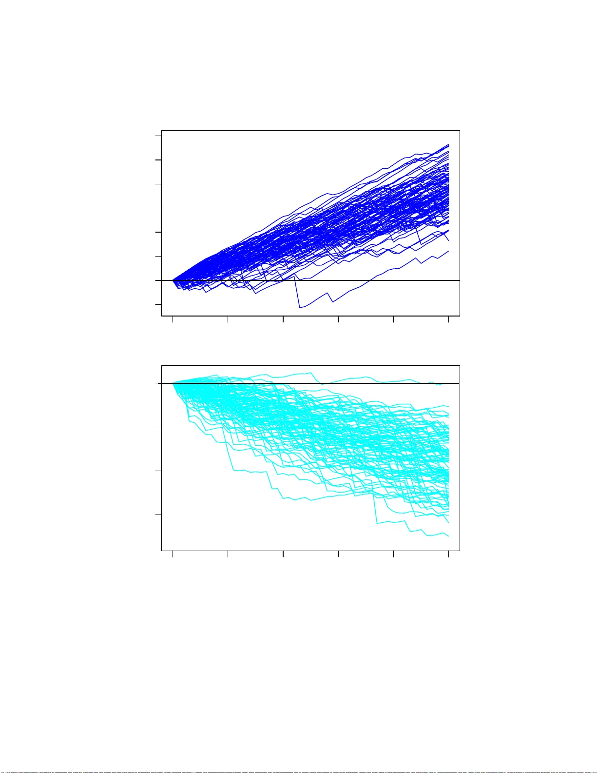
A defense of Colum b o (and of the use of Ba y esian inference in fo rensics) – A mu ltilevel in tro duction to probabilistic r easoning – G. D’Agostini Univ ersit` a “L a Sapien za” and INFN, Roma, Italia (giulio.dagos tini@roma1.infn.it, http:/ /www.roma1. i nfn.it/ ~ dagos ) Abstract T riggered b y a recent in tere s ting New Scient ist ar ticle on the to o fre q uen t incorr ect use of proba bilistic evidence in courts, I introduce the basic co nce pts of proba bilis- tic inference with a toy mo del, and discuss several imp ortant issues that need to b e understo od in order to extend the basic reasoning to r eal life cases. In par ticular, I emphasize the often neg lected point that degrees of beliefs are up dated not by ‘bare facts’ alone, but by all av ailable information p ertaining to them, including how they hav e b een acquired. In this lig ht I s ho w that, contrary to what claimed in that ar ticle, there was no “proba bilis tic pitfall” in the Columbo’s episo de p oin ted a s example of “bad mathematics” yielding “rough justice”. Instead, such a cr iticism could hav e a ‘negative reaction’ to the article itself and to the use of Bayesian rea soning in courts, as w ell as in all other places in which probabilities need to be a s sessed and decisio ns need to b e made. Anyw ay , besides in tro ductory/recr eational asp ects, the pa per touches impo rtan t questions , like: role and ev aluation of prior s; sub jective ev aluatio n of Bayes factors; r ole a nd limits of intuition; ‘weight s of evidence’ and ‘intensities of b eliefs’ (fol- lowing Peirce) a nd ‘judgments leaning’ (here introduced), including their uncerta inties and combinations; role of r elativ e freq uencies to as sess a nd express b eliefs; pitfalls due to ‘standar d’ statistical e ducation; w eight o f evidences mediated by testimonies. A small in tro duction to Bay esian netw ork s, based on the same toy mo del (complicated by the p ossibility of incorrect testimonies) and implement ed us ing Hugin softw are, is a lso provided, to str ess the imp ortance o f for mal, c omputer aided pro babilistic reaso ning. “Use eno ugh c ommon sense to k no w when ordinary common se nse do es no t apply” (I.J. Go od’s guiding p rinciple of al l scienc e ) 1 Figure 1 : Peter Galesco, p l a yed by Dick Van Dyke, tak i ng the picture of its wife b efore killing her. 1 In tro duc tion A r ec en t New Scien tist article [1] deals with errors in courts d ue to “b ad mathematics”, adv o cat ing the use of the so-called Ba y esian metho ds to a v oid them. Although most ex- amples of resulting “rough jus ti ce” come from real life cases, the ﬁrst “p r obabilistic p itfal l” is tak en from cr im e ﬁction, namely fr om a “1974 episo de of th e cult US television series” Columb o , in wh ic h a “so cie t y p h oto grapher has killed his wife and disguised it as a bungled kidnapping.” The pretended mistak e happ ens i n the concluding sce ne, when “the hangdog detectiv e [. . . ] in duces the m urderer to grab f r om a shelf of 12 cameras the exact one used to snap the victim before she w as killed.” According to the a rticle author (or to experts on whic h scien tiﬁ c journ alist s ofte n rely on) the qu estio n is that “killer or not, any one w ould ha ve a 1 in 1 2 c hance of picking th e same camera at random. That kind o f evidence w ould neve r stand up in court.” Then a sad doubt is raised, “Or w ould it? In fact, such probabilistic pitfalls a re not limited to crime ﬁction.” Being myse lf not p artic ularly fond of this kind of ente rtainment (p erhaps w it h a little exception of the Colum b o series, that I w atc h casually), I cannot tell how muc h crime ﬁction literature and m o vies are aﬀected by “probabilistic p itfal ls”. Instead, I can giv e ﬁ rm witness that scient iﬁc practice is p lent y of mistak es of the kind r ep orted in Ref.[1], that happ en ev en in ﬁ elds the general p ublic would hardly susp ect, lik e front ier physics, w hose protagonists are su pp osed to hav e a skill in mathematics sup erior to p olice oﬃcers and la wyers. But it is not ju s t a question of math skill (complex calculations are usually done without mistak es), bu t of pr ob abilistic r e asoning (what to calculate!). This is a quite old story . In 2 fact, as Da vid Hum e complained 260 ye ars ago [2], ”The celebrated Monsieur Leibniz h as observe d it to b e a defect in th e common systems of logic, that they are v ery copious when they explain the op eratio ns of the und erstanding in the forming of d emons trat ions, b ut are to o concise when they treat of probabilities, an d those other measures of evidence on whic h life an d action en tirely d epend , and whic h are our guides eve n in most of our philosophical sp eculations.” It seems to me that the general situation has not improv ed muc h. Y es, ‘statistics’ (a name that, meaning to o muc h , risks to m ea n little) is taugh t in colleges and un iversities to student s of several ﬁelds, bu t distorted by the ‘frequentisti c approac h’, according to which one is not allo wed to sp eak of probabilities of causes. This is, in m y opinion, the original sin that giv es grounds for a large num b er of pr obabilisti c mistak es ev en by otherwise very v aluable scien tists and practitioners (see e.g. chapter 1 of Ref. [3 ]). Going bac k to the “sh am bling sleuth Columb o” , b eing m y wife and m y daught er his fans, it h appen s we own th e DVD collec tions of the ﬁrst sev en seasons. It o ccurred then I wa tc hed with them, not m uch time ago (p erhaps last winte r), the ‘incriminated’, su p erb episo de N e gative R e action [4], one of the b est p erformances of Pet er F alk pla ying the r ol e of the famous lieutenan t. Ho wev er, r ea ding th e m en tioned New S cie nt ist article, I did not remem b er I had a ‘n egativ e reaction’ from the ﬁ nal scene, although I use and teac h Ba y esian metho ds for a large v ariety of applications. Did I ov erlo ok something? I w atc hed again th e episo de and I w as aga in convinced Columb o’s last mo ve was a conclusiv e c heckmate . 1 Then I ha v e in vited some f riends, all with physics or mathematics degree and somewhat knowledgea ble of the Ba yesia n approac h, to enjoy an ev enin g together during th e r ec en t end of yea r holidays in ord er to let them make up th ei r minds whether Colum b o had go od reasons to tak e P aul Galesco, magniﬁcen tly imp ersonated by Dic k V an Dyk e, in front of the court (Ba y es or n o t, w e had some f u n. . . ). The v erdict was unanimous : Colum b o w as fully absolve d or, more precisely , th ere was nothing to repr oa c h the story writer, P eter S. Fisc her. The convivial after dinner jury also requested me to write a n ot e on the qu esti on, p ossibly with a short, self-con tained in tro duction to th e ‘required math’. Not only to ‘defend Colum b o’ or, more prop erly , his writer, but, and more seriously , to defend the Ba y esian appr oa c h, an d in particular its applications in foren s ic science. In fact, we all deemed the b eginning paragraph s of the New Scien tist article could thro w a bad ligh t on the r est of the con ten ts. Imagine a casual reader of the article, p ossibly a lawy er, a jud ge or a student in forens ic science, to wh ich th e article was virtually addressed, and wh o might ha v e seen Ne gative R e action . Most lik ely he/she considered legitimate the charges of the p olicemen against the 1 Just writing this note, I hav e realized that the ﬁnal scene is directed so w ell that, not only th e w ay the photographer loses control and commits his fatal mistake looks very credible, bu t also sp ectators forget he could play v alid countermo ves, not d ep ending on the negative of the preten ded destro yed picture (see footnote 32). Therefore, rather than chess, th e name of the game is p oker , and Columbo’s blu ﬀ is able to induce the murderer to provide a crucial p iece of evid ence to ﬁnally incriminate him. 3 photographer. T he ‘negativ e reaction’ would b e that the r eader w ould consider the r est of the article a supp ort of du bious v alidit y to some ‘strange math’ that can nev er su bstitute the h uman in tu ition in a trial. 2 Not a go o d service to the ‘Ba yesia n cause’. (Imagine someb od y tryin g to convi nce y ou with arguments you hardly understand and who b egins asserting something yo u consid er manifestly false.) In th e f ol lo wing section I introdu ce the basic element s of Ba yesia n reasoning (sub sect ion 2.4 can b e skipp ed on ﬁrst reading), using a to y mo del as guid ing example in which the analysis of ref. [1] (“1 in 12”, or, m ore pr ec isely “1 in 13”) holds. S ect ion 4 sho ws h o w su c h a kind of evid en ce would change Colum b o’s and jury’s opinion. T hen I discu ss in s ec tion 5 wh y a similar argument do es n ot app ly to the clip in whic h Columb o ﬁn a lly frames Galesco, and why all witnesses of th e crucial actions (includin g TV watc hers, with the exception of the author of Ref. [1] and p erhaps a f ew others) and an hyp othetic al court jur y (pr o vided the scene h ad b een p r operly r eported) h ad to b e absolutely p ositiv e th e photographer killed his wife (or at least he knew wh o did it in his p lace). The rest of the p aper might b e marginal, if you are just cur io us to k n o w why I ha v e a diﬀeren t opinion than Ref. [1], although I agree on the v alidit y of Ba yesian reasoning. In fact, at the en d of th e wo rk, this p aper is n ot th e ‘short n ote’ initially plann ed. The r ea son is that the past mont hs I had m an y d iscussions on s ome of the questions treated her e with p eople from seve ral ﬁelds. I ha v e realized once more that it is not easy to p ut the basic principles at wo rk if some imp ortant issues are not wel l un derstoo d. Peo ple are used to solving their statistical p roblems with ‘ad ho c’ formulae (see Ap p end ix H) and therefore tend to add some ‘Ba yesian recip es’ in their formularium. It is then to o high the risk that one lo oks at simpliﬁed metho ds – Ba y esian m et ho ds requ ire a bit m ore thinking and computation that others! – that are eve n adv ertised as ‘ob jectiv e’. Or one just refu ses to use any math, on the d efense of p u re in tuition. (By th e w a y , this is an imp ortan t p oint and I will tak e th e opp ortunit y to comment on the apparent con tradictions b et wee n intuitio n and formal ev aluation of b eliefs, defendin g . . . b oth, but encouraging the use of th e latter, sup erior to the f ormer in complex situations – see in particular App endix C). So, to conclude the introdu ct ion, this do cument oﬀers sev eral leve ls of r ea ding: • If yo u are only interested to C olum b o’s story , you can just ju m p straight to section 5. • If yo u also (or regardless of C o lumb o) w an t to ha ve an opp ortunit y to learn the basic rules of Ba y esian inferen ce , sub sect ions 2.1 , 2.2 an d 2.3, based on a simple master example, ha v e b een written on the pur pose. Then y ou might appreciate the adv an tage of logarithmic up dating (section 2.4) and p erhaps see ho w it app lie s to the AIDS examp le of Ap p end ix F. 2 This kind of ob jection, in defense of what is often nothing bu t “the capricious ipse dixit of authorit y”[5], from which we should instead “emancipate”[5 ], is quite frequent. It is raised not only by judges, who tend to claim t h eir job is ”to ev aluate ev idence not by means of a formula... bu t by the joint application of their individu al common sense.”[1], but also by other categories of p eople who take important decisions, like doct ors , managers and p oliticians. 4 • If y ou already kno w the basics of the probabilistic reasoning, but y ou wonder how it can b e app lie d into real cases, then section 3 s hould help, together with some of the app endices. • If none of the p revious cases is yours (y ou migh t eve n b e an exp ert of the ﬁeld), you can s imply bro wse the d ocument. P erhaps some app end ice s or sub sec tions might s till b e of y our interest. • Finally , there is the question of the many fo otnotes, w hic h can break the pace of the reading. They are not mean t to b e n ec essarily read sequen tially along with the main text and could b e skipp ed on a ﬁrst fast reading (in fact, this do cumen t is closer to an hyp ertext than to a standard article.) Enjo y! 2 One in thirteen – Ba y esian reasoning illustrated with a to y mo del Let us lea ve aside Columb o’s cameras for a while and b egin with a diﬀerent , sim p ler, stereot yp ed situ ation easier to analyze. Imagine th ere are t w o t yp es of b o xes, B 1 , that only con tain wh ite balls ( W ), and B 2 , that con tain one wh ite b all s and t w elv e blac k (incidenta lly , ju st to b e precise, although the detail is absolutely irrelev an t, w e hav e to inf er from Columb o’s wo rds, “Y ou didn ’t touch any of these twelve c amer as. Y ou picke d up that one” , the cameras were th ir te en). Y ou take at rand om a b o x and extract a ball. The resulting color is white . Y ou migh t b e in terested to ev aluate the p robabilit y that the b o x is of t yp e B 1 , in the sense of s ta ting in a quan titativ e w a y h o w m uch you b eliev e this h yp othesis. In formal terms we are in terested in P ( B 1 | W, I ), kn o wing that P ( W | B 1 , I ) = 1 and P ( W | B 2 , I ) = 1 / 13, a problem that can b e sketc hed as  P ( W | B 1 , I ) = 1 P ( W | B 2 , I ) = 1 / 13 ⇒ P ( B 1 | W, I ) = ? (1) [Here ‘ | ’ stands for ‘giv en’, or ‘conditioned by’; I is th e general (‘bac kground’) status of information und er whic h this probab ility is assessed; ‘ W , I ’ or ‘ B i , I ’ after ‘ | ’ ind ica tes that b oth conditions are relev an t for the ev aluation of the probabilit y .] A typical mistak e at this p oin t is to confuse P ( B 1 | W, I ) with P ( W | B 1 , I ), or, more often, P ( B 2 | W, I ) with P ( W | B 2 , I ), as largely discussed in Ref. [1 ]. Hence w e need to learn ho w to turn p rop er ly P ( W | B 1 , I ) in to P ( B 1 | W, I ) u sing the rules of probabilit y theory . 5 2.1 Ba y es t heorem and Ba y es factor The ‘pr obabilisti c inv ersion’ P ( W | B 1 , I ) → P ( B 1 | W, I ) can only 3 b e p erformed using the so-calle d Bayes’ the or em , a s im p le consequence of the fact that, giv en the eﬀe c t E and some hyp otheses H i concerning its p ossible cause, th e joint probabilit y of E and H i , conditioned b y the b ackgr ound information 4 I , can b e written as P ( E ∩ H i | I ) = P ( E | H i , I ) · P ( H i | I ) = P ( H i | E , I ) · P ( E | I ) , (2) where ‘ ∩ ’ stands for a logical ‘AND’. F rom the second equalit y of the last equation we get P ( H i | E , I ) = P ( E | H i , I ) P ( E | I ) · P ( H i | I ) , (3) that is one of the wa ys to exp ress Ba y es’ theorem. 5 Since a sim ilar expr ession h ol ds for an y other hyp ot hesis H j , d ividing member by m em- b er the tw o expr essions we can restate the theorem in terms of the relativ e b eliefs, that is P ( H i | E , I ) P ( H j | E , I ) | {z } up dated o dds = P ( E | H i , I ) P ( E | H j , I ) | {z } up dating factor (‘ Bayes f actor ’) × P ( H i | I ) P ( H j | I ) | {z } initial o dds : (4) the initial ratio of b eliefs (‘od ds’) is up dated by th e so-called Bayes factor , th at dep ends on how lik ely e ach hypothesis can pro duce that eﬀect. 6 In tro ducing O i,j and BF i,j , w ith ob vious meanings, we can rewrite E q . (4) as O i,j ( E , I ) = BF i,j ( E , I ) × O i,j ( I ) . (5) 3 Bew are of metho ds that provide ‘levels of conﬁdence’, or something like that, without using Ba yes’ theorem! See also fo otnote 9 and A ppendix H. 4 The background information I rep rese nts all we k no w ab out the hypoth ese s and the eﬀect considered. W riting I in all expressions could seem a p edantry , but it isn’t. F or ex amp le , if we w ould just write P ( E ) in these formula e, instead of P ( E | I ), one migh t b e tempted to take this probabilit y eq u al to one, “b ecause the observed even t is a well established fact’, that h as happ ened and is then certain. But it is not this certain ty that enters these form ulae, but rather the probabilit y ‘that fact could happ en’ in the ligh t of ‘everything w e knew’ ab out it (‘ I ’). 5 Ba yes’ theorem can b e often found in th e form P ( H i | E , I ) = P ( E | H i , I ) · P ( H i | I ) P i P ( E | H i , I ) · P ( H i | I ) , v alid if we deal with a class of incompatible hypotheses [i.e. P ( H i ∩ H j | I ) = 0 and P i P ( H i | I ) = 1]. In fact, in this case a general rule of p robabil ity theory [Eq. (35) in A ppendix A] allo ws us to rewrite th e denominator of Eq. (3) as P i P ( E | H i , I ) · P ( H i | I ). In this note, dealing only with tw o hypotheses, we prefer to reason in terms of probability ratios, as shown in Eq. (4). 6 Note that, while in the case of only tw o hyp otheses entering the in ferential game their initial p robabili ties are related by P ( H 2 | I ) = 1 − P ( H 1 | I ), t he probabilities of the eﬀects P ( E | H 1 , I ) and P ( E | H 2 , I ) hav e usually nothing to do with each oth er. 6 Note that, if th e initial o dds are unitary , than the ﬁn al o dds are equal to the u p dating factor. Then , Bayes f a ctors c an b e interpr ete d as o dds due only to an individual pie c e of evidenc e, if the two hyp otheses wer e c onsider e d i nitial ly e qual ly likely . 7 This allo w s us to rewrite BF i,j ( E , I ) as ˜ O i,j ( E , I ), where the tilde is to remind th at they ar e not pr op erly o dds , bu t rather ‘ pseudo-o dds ’. W e get then an expr essio n in wh ic h all terms hav e virtual ly uniform meaning: O i,j ( E , I ) = ˜ O i,j ( E , I ) × O i,j ( I ) . (6) If w e ha ve only t w o hypotheses, w e get simply O 1 , 2 ( E , I ) = ˜ O 1 , 2 ( E , I ) × O 1 , 2 ( I ) . If the up dating factor is unitary , then the p iec e of evidence d oes n ot mo dify our opinion on the t wo h yp otheses (no matter ho w small can numerator and den o minator b e, as long as th eir r atio remains ﬁnite and unitary! – see App endix G for an example wo rke d out in d eta ils); wh en ˜ O 1 , 2 ( E , I ) v anishes, then hypothesis B 1 b ecomes imp ossible (“ it is falsiﬁe d ”); if instead it is in ﬁnite (i.e. the d enominato r v anishes), then it is the other hyp othesis to b e imp ossible. (The un deﬁned case 0 / 0 means that we h a v e to lo ok for other hypotheses to explain the eﬀect. 8 ) 2.2 Role of priors Applying the up dating r ea soning to our b o x game, th e Ba y es factor of interest is ˜ O 1 , 2 ( W , I ) = P ( W | B 1 , I ) P ( W | B 2 , I ) = 1 1 / 13 = 13 . (7) As it wa s remark ed, this num b er wo uld giv e the required o dds if the hypotheses we re ini- tially equally likel y . But ho w strong are the initial relativ e b eliefs on the t wo hyp otheses? ‘Unfortunately’, we cannot p erform a probabilistic inv ersion if w e are unab le to assign some- ho w prior pr ob abilities to the hyp otheses we are in terested in. 9 Indeed, in the formulatio n 7 Those who wa nt to base the inference only on the p robabili ties of the observ ations given the hypotheses, in order to “let the data sp eak themselves” , might b e in go od faith, but their noble inten tion do es dot sa ve them from d ire mistakes [3]. (See also fo otnotes 9 and 43 , as well as Ap pendix H.) 8 Pieces of ev idence mo dify , in general, relativ e b eliefs. Wh en we turn relative b eliefs into absolute ones in a scale ranging from 0 to 1, we are al w ays making th e implicit assumption t h at the p ossi ble hyp otheses are only those of the class considered. If other hypotheses are added, th e relative b elief s do not change, while the absolute on es do. This is the reason why an hypoth esis can even tually b e falsiﬁed, if P ( E | H i , I ) = 0, but an absolute tru th, i.e. P ( E | H j , I ) = 1, dep ends on which class of hyp otheses is considered. Stated in other w ords, in the realm of probabilistic inference falsities c an b e absolute, but truths ar e always r elative . 9 Y ou might b e reluctant to adopt th is wa y of reasoning, ob jecting “I am unable to state priors!”, or “I don’t wan t to b e inﬂuenced by prior!”, or even “I don’t wan t to state degrees of b eliefs, but only real probabilities”. N o problem, provided you stay aw ay from probabilistic inference (for example you can enjo y ﬁshing or hiking – bu t I hop e you are aw are of t he large amount of p rio r b eliefs inv olved in these activities too!). Here I can only advice you, provided you are interested in ev aluating p robabili ties of ‘causes’ from eﬀects, not to ov erlo ok prior information and not to b li ndly trust statistical meth o ds and soft w are pack ages advertise d as p rio r-free, unless yo u d on’t w ant to risk to arrive at ve ry bad conclusions. F or more comments on the q uestion see Ref. [3], fo otnote 43 an d App endix H. 7 Figure 2: Graphical representation o f th e causal connections Box → E i , where E i ar e the eﬀects (White/Black a t each extractio n). Th e se eﬀects are then causes o f other eﬀects ( E i T ), the rep orted colors, where ‘ T ’ stands for ‘testimon y’. T he arro ws connecting the var ious ‘no des’ represent c o nditional pr obabi l ities. The mo del will b e full y exploited in App endix J. of the problem I on purp ose p a ssed o v er the relev an t pieces of information to ev aluate the prior probabilities (it w as said that “there are t w o t yp es of b o xes”, n ot “there are tw o b o xes”!). If we sp ecify that we h ad n 1 b o xes of typ e B 1 and n 2 of the other kind, then the initial o dds are n 1 /n 2 and the ﬁnal ones will b e O 1 , 2 ( W , I ) = ˜ O 1 , 2 ( W , I ) × O 1 , 2 ( I ) (8) = 13 × n 1 n 2 , (9) from whic h we get (just r equ iring that the probabilit y of the tw o hyp otheses ha v e to su m up to one 10 ) P ( B 1 | W, I 0 ) = 13 13 + n 2 /n 1 . (10) If th e t wo hyp otheses were initial ly considered equally lik ely , then the evidence W mak es B 1 13 times more b eliev able than B 2 , i.e. P ( B 1 | W, I 0 ) = 13 / 14, or approxi mately 93%. On the other h and, if B 1 w as a priori muc h less credible than B 2 , for example by a factor 10 If H 1 and H 2 are generic, complementary hypotheses we get, calling b the Bay es factor of H 1 versus H 2 and x 0 the initial o dds to simplify the notation, the follo wing conve nient expressions to ev aluate the probabilit y of H 1 : P ( H 1 | x 0 , b ) = b x 0 1 + b x 0 = b b + 1 /x 0 = x 0 x 0 + 1 /b . 8 13, ju st to pla y with roun d num b ers, the same evidence made B 1 and B 2 equally lik ely . Instead, if we were initially in strong f av or of B 1 , considering it for instance 13 times more plausible than B 2 , that evidence tur ned this factor into 169, making us 99.4% conﬁdent – highly c onﬁdent , some would even say ‘practically sur e’ ! – that the b o x is of t yp e B 1 . 2.3 Adding pieces of evidence Imagine now the follo wing v arian t of the previous to y exp eriment. After the w h ite ball is observ ed, you put it again in the b o x, shake w ell and make a second extraction. Y ou get white the second time to o. Calling W 1 and W 2 the t w o observ ations, w e hav e now: 11 P ( B 1 | W 1 , W 2 , I 0 ) P ( B 2 | W 1 , W 2 , I 0 ) = P ( W 1 , W 2 | B 1 , I 0 ) P ( W 1 , W 2 | B 2 , I 0 ) × P ( B 1 | I 0 ) P ( B 2 | I 0 ) (11) = P ( W 2 | W 1 , B 1 , I 0 ) · P ( W 1 | B 1 , I 0 ) P ( W 2 | W 1 , B 2 , I 0 ) · P ( W 1 | B 2 , I 0 ) × P ( B 1 | I 0 ) P ( B 2 | I 0 ) (12) = P ( W 2 | B 1 , I 0 ) P ( W 2 | B 2 , I 0 ) × P ( W 1 | B 1 , I 0 ) P ( W 1 | B 2 , I 0 ) × P ( B 1 | I 0 ) P ( B 2 | I 0 ) (13) = P ( W 2 | B 1 , I 0 ) P ( W 2 | B 2 , I 0 ) × P ( B 1 | W 1 , I 0 ) P ( B 2 | W 1 , I 0 ) , (14) that, using the compact n ot ation in tro duced ab o ve, we can r ewrite in th e follo wing enligh t- ing forms. Th e ﬁrst is [Eq. (14)] O 1 , 2 ( W 1 , W 2 , I ) = ˜ O 1 , 2 ( W 2 , I ) × O 1 , 2 ( W 1 , I ) , (15) that is, the ﬁnal o dds after the ﬁrst infer enc e b e c ome the ini tial o dds of the se c ond infer enc e (and so on, if there are sev eral pieces of evidence). Therefore, b eginning from a situation in whic h B 1 w as thirteen times more credible than B 2 is exactly equiv alen t to ha ving started from unitary o dds u pd at ed by a f actor 13 due to a piece of evidence. The second form comes fr om Eq. (13): O 1 , 2 ( W 1 , W 2 , I ) = ˜ O 1 , 2 ( W 1 , I ) × ˜ O 1 , 2 ( W 2 , I ) × O 1 , 2 ( I ) (16) = ˜ O 1 , 2 ( W 1 , W 2 , I ) × O 1 , 2 ( I ) , (17) i.e. 12 ˜ O 1 , 2 ( W 1 , W 2 , I ) = ˜ O 1 , 2 ( W 1 , I ) × ˜ O 1 , 2 ( W 2 , I ) : (18) 11 Note that w e are still using Eq . (4), although we are d ea ling now with more complex even ts and complex hypotheses, logical AN D of simpler ones. Moreov er, Eq . (12 ) is obtained from Eq. (11 ) making use of the form ula (2 ) of joint probability , that gives P ( W 1 , W 2 | B 1 , I ) = P ( W 2 | W 1 , B 1 , I ) × P ( W 1 | B 1 , I ) and an analogous formula for B 2 . Note also th at, going from Eq . (12) to Eq. (13), P ( W 2 | W 1 , B i , I 0 ) has b een rewritten as P ( W 2 | B i , I 0 ) t o emphasize th at the probability of a second white ball, conditioned by the b ox composition an d the result of the ﬁ rst ex t racti on, dep ends ind eed only on the b o x conten t an d not on the previous outcome (‘extraction after re-introduction’). 12 Eq. (17) follo ws from Eq. (16) b ecause a Bay es factor can b e deﬁned as the ratio of ﬁn al o dds ov er the 9 Bayes factors due to indep endent 13 pieces of evidence multiply . Th at is, tw o indep endent pieces of evidence ( W 1 and W 2 ) are equiv alent to a single p iec e of evidence (‘ W 1 ∩ W 2 ’), whose Ba y es factor is the p rodu ct of th e individual ones. In our case ˜ O 1 , 2 ( W 1 ∩ W 2 , I ) = 169. In general, if w e hav e seve ral hyp otheses H i and several indep endent pieces of evidence, E 1 , E 2 , . . . , E n , indicated all together as E , then Eq. (4) b ecomes O i,j ( E , I ) = " n Y k =1 ˜ O i,j ( E k , I ) # × O i,j ( I ) , (19) i.e. ˜ O i,j ( E , I ) = n Y k =1 ˜ O i,j ( E k , I ) , (20) where Q stand for ‘pr o duct’ (analogous to P for sums). 2.4 Ho w the indep enden t argumen ts sum up in our judgemen t – loga- rithmic up dating and its in t erpretation The remark that Ba y es factors du e to indep endent pieces of evidence multiply together and the o v erall f a ctor ﬁ nally m ultiplies the initial o dds suggests a c hange of v ariables in order to p la y with additive quantit ies. 14 This can b e done taking th e logarithm of b oth sid es of Eq. (19), that then b ecome log 10 [ O i,j ( E , I )] = n X k =1 log 10 [ ˜ O i,j ( E k , I )] + log 10 [ O i,j ( I )] , (21) initial od ds, dep ending on the evidence. Therefore ˜ O 1 , 2 ( W 1 , W 2 , I ) = O 1 , 2 ( W 1 , W 2 , I ) O 1 , 2 ( I ) = ˜ O 1 , 2 ( W 1 , I ) × ˜ O 1 , 2 ( W 2 , I ) . 13 Probabilistic, or ‘sto chastic’, indep endence of the observ ations is related to the val idity of th e relation P ( W 2 | W 1 , B i , I ) = P ( W 2 | B i , I ), that we hav e used ab o ve to tu rn Eq . (12) into Eq. (13) and that can b e expressed, in general terms as P ( E 2 | E 1 , H i , I ) = P ( E 2 | H i , I ) , i.e., under the c ondition of a wel l pr e cise hyp othesis ( H i ), the probability of the eﬀect E 2 does not dep end on t he knowledge of wheth er E 1 has o ccurred or not. Note that, in general, although E 1 and E 2 are indep enden t giv en H i (they are said t o b e c onditional ly indep endent ), they might b e otherwise dep endent , i.e. P ( E 2 | E 1 , I 0 ) 6 = P ( E 2 | I 0 ). (Going to the examp le of th e b o x es, it is rath er easy to grasp, althou gh I cannot enter in details here, th at, if we do not know the kind of b o x, the observ ation of W 1 changes our opinion about the box comp osition and, as a consequence, t h e probabilit y of W 2 – see the examples in App endix J) 14 The idea of transforming a multiplicativ e u p dating in to an additive one via the use of logarithms is quite natural and seems to h a ve b een ﬁrstly u sed in 1878 by Charles Sanders Peirce [6] and ﬁ nally introduced in the statistical practice mainly due to th e wo rk of I.J. Go od [7]. F or more details see the App endix E. 10 0 2 4 6 8 10 -2 -4 -6 -8 -10 J L Figure 3: Judgem e n t lea ning. resp ectiv ely , where the base 10 is chosen for practical conv enience b ecause, as w e s hall discuss later, wh at s ubstan tially matters are p ow ers of ten of the o dds. In tro ducing the new symb ol JL, we can rewrite Eq. (21 ) as JL i,j ( E , I ) = JL i,j ( I ) + n X k =1 ∆JL i,j ( E k , I ) (22) = JL i,j ( I ) + ∆JL i,j ( E , I ) (23) or ∆JL i,j ( E , I ) = JL i,j ( E , I ) − JL i,j ( I ) , (24) where JL i,j ( E , I ) = log 10 [ O ij ( E , I )] (25) JL i,j ( I ) = log 10 [ O i,j ( I )] (26) ∆JL i,j ( E k , I ) = log 10 h ˜ O i,j ( E k , I ) i (27) ∆JL i,j ( E , I ) = n X k =1 ∆JL i,j ( E k , I ) . (28) The letter ‘L’ in the s ym b ol is to remind lo garithm . But it h as also the mnemonic meaning of le aning , in the s en se of ‘inclination’ or ‘p rop en sion’. Th e ‘J’ is for judgment . Therefore ‘JL’ stands for judgement le aning , that is an inclination of the judgement , an expression I ha v e tak en the lib ert y to int ro duce, using words n ot already engaged in p robabilit y and statistics, b ecause in these ﬁelds many con tro ve rsies are d ue to d iﬀeren t meanings attributed to the same word, or expr ession, b y diﬀerent p eople (see App endices B and G f or further commen ts). JL can th en b e visualized as the indicator of the ‘justice balance’ 15 (ﬁgure 15 I hav e realized only later that JL sounds a bit like ‘jail’. That might b e not so b ad, if H 1 to which JL 1 , 2 ( E k ) refers stands for ‘guilty’. 11 3), that d ispla ys zero if there is no unbalance, but it could m o v e to the p ositiv e or the negativ e side dep ending on the w eigh t of the sev eral arguments p ro and con. Th e r ole of the evidence is to v ary the JL in d ica tor b y quantit ies ∆JL’s equal to base 10 logarithms of the Ba y es factors, that hav e th en a meaning of weig ht of evidenc e , an exp ression due to Charles Sanders Peirce [6] (see App end ix E). But the judgement is rarely initially unbalanced. This the role of J L i,j ( I ), that can b e considered as a a kind of initial weight of evi d enc e du e to our pr io r kno wledge ab out the h yp otheses H i and H j [and that could ev en b e wr itt en as ∆JL i,j ( E 0 , I ), to stress that it is related to a 0-th piece of evidence] T o und erstand the rationale b ehind a p ossible u niform treatmen t of the pr io r as it would b e a piece of evidence, let u s start from a case in wh ic h y ou no w absolutely nothing . F or example Y ou ha v e to state your b eliefs on which of my friends, Dino or Pao lo, w ill ﬁrst run next Rome marathon. It is absolutely reasonable you assign to the tw o hypotheses equal probabilities, i.e. O 1 , 2 = 1, or JL 1 , 2 = 0 (y our judgement is p erfectly balanced). Th is is b ecause in Y our brain these names are only p ossibly related to Italian males. Nothing more. (But no w ada ys searc h engines ov er the w eb allo w to mo dify y our opinion in minutes.) As so on as yo u d ea l with r e al hypotheses of y our inte rest, things get quite diﬀerent. It is in fact very rare the case in wh ic h the hyp otheses tell y ou not more than th eir names. It is enough y ou thin k at the hyp otheses ‘rain’ or ‘n ot rain’, the d a y after yo u read these lines in the place w here you liv e. I n general the in formatio n yo u ha v e in yo ur brain r ela ted to the h yp otheses of your in terest can b e considered the in itial piece of evidence you hav e, usually diﬀeren t from that someb o d y else might ha v e (this the role of I in all our expressions). I t follo ws that p rior o dds of 10 (JL = 1) w ill inﬂu ence y our leaning tow ards one hypothesis, exactly like u nitary o dds (JL = 0) follo w ed by a Ba yes factor of 10 (∆JL = 1). This the reason they enter on equal fo ot w hen “balancing argument s” (to use an expr ession ` a la P eirce – see the App end ix E) pr o and against h yp otheses. Finally , table 1 compares j udgemen ts leanings, o dds and pr ob ab ilities, to show that th e h uman sen s iti vit y to b elief (that is something lik e P eirce’s intensity of b elief – see App endix E) is not linear with p robabilit y . F or example, if w e assign probabilities of 44%, 50% or 56% to ev ents E 1 , E 2 and E 3 w e d o not exp ect one of them really more s trongly th an the others, in the sense th at w e are not m uc h surprise d of any of the three o ccurs. But the same diﬀerences in probabilit y pro duce qu ite d iﬀe rent sentiment of surprise if w e shift the probabilit y s ca le (if they we re, instead, 1%, 7% and 13%, we w ould b e highly sur prised if E 1 o ccurs). Similarly 99.9% probab ility on H is substantia lly diﬀerent from 99.0%, although the diﬀerence in probabilit y is ‘only’ 0.9%. This is well understo o d, and in fact it is known that the b est wa y to express the p erception of probabilit y v alues very close to 1 is to think to the opp osite h yp othesis H , that is 0.1% pr obable in the ﬁrst case and 1% probab le in the second – we could b e qu ite diﬀerently s u rprised if H d oes not result to b e true in the tw o cases! 16 16 The ‘switc h of p erspective’ from E to H is d one in a w ay somewhat automatic if, instead of the 12 Judg. leaning Odds(1:2) P ( H 1 ) Judg. leaning Odd s(1: 2) P ( H 1 ) [JL 1 , 2 ] [ O 1 , 2 ] (%) JL 1 , 2 ] [ O 1 , 2 ] (%) 0 1.0 50 − 0 . 1 0.79 44 0 . 1 1.3 56 − 0 . 2 0.63 39 0 . 2 1.6 61 − 0 . 3 0.50 33 0 . 2 2.0 67 − 0 . 4 0.40 28 0 . 4 2.5 71 − 0 . 5 0.32 24 0 . 5 3.2 76 − 0 . 6 0.25 20 0 . 6 4.0 80 − 0 . 7 0.20 17 0 . 7 5.0 83 − 0 . 8 0.16 14 0 . 8 6.3 86 − 0 . 9 0.13 11 0 . 9 7.9 89 − 1 . 0 0.10 9.1 1 . 0 10 91 − 1 . 1 0.079 7.4 1 . 1 13 92.6 − 1 . 2 0.063 5.9 1 . 2 16 94.1 − 1 . 3 0.050 4.7 1 . 0 20 95.2 − 1 . 4 0.040 3.8 1 . 4 25 96.2 − 1 . 5 0.032 3.1 1 . 5 32 96.9 − 1 . 6 0.025 2.5 1 . 6 40 97.5 − 1 . 7 0.020 2.0 1 . 7 50 98.0 − 1 . 8 0.016 1.6 1 . 8 63 98.4 − 1 . 9 0.013 1.2 1 . 9 80 98.8 − 2 . 0 0.010 1.0 2 . 0 100 99.0 T able 1: A co m p a riso n b et ween probabilit y , o dds and judg ement leanings F rom the table w e can see that the human r esolution is ab out 1/10 of th e JL, although this d oes n ot imp ly that a probability v alue of 53.85% (JL = 0 . 0670) cannot b e stated. It all dep ends h ow th is v alue has b een ev aluated and what is the purp ose of it. 17 probabilit y , we t ak e the logarithm of the o dds, for example our JL (obviously t he base of the logarithm is irrelev ant). Since JL H ( I ) = log 10 [ P ( H | I ) /P ( H | I )], in the limit P ( H | I ) → 0 we hav e that JL H ( I ) ≈ log 10 [ P ( H | I )], while the limit P ( H | I ) → 1 it is JL H ( I ) ≈ − log 10 [ P ( H | I )]. 17 This is more or less what h appens in measurements. T ak e for example the probabilities that app ears in the E 1 ‘monitor’ of ﬁgure 11: 53.85% for white and 46.15% for b lack. This is like to sa y that tw o b od ies w eigh 53.85 g and 46.15 g, as resulting from a measurement with a precise balance (the Bay esian n et work tool describ ed in App endix J app li ed t o the b o x t oy model is th e analogue of the precise balance). F or some purp oses tw o, three and even four signiﬁcant digits can b e important. But, an yhow, as far as our p erception is concerned, not only the least digits are absolutely irrelev ant bu t w e can hardly distinguish b et ween 54 g and 46 g. 13 2.5 Recap of the sect ion This section h ad th e purp ose of introdu cing the so-called Ba yesian reasoning (that is, in realit y , nothing more than just probab ilistic reasoning) with an aseptic, simp le example, that sho ws how ev er the in gredien ts n eeded to up date our opinion on the ligh t of new observ ations. A t th is p oin t the role of the priors and of the eviden ce in formin g our opinion ab out the hypotheses of interest should b e clear. Note also how I hav e used on purp ose sev eral expressions to mean essen tially the same thing, expressions that inv olv e words such as ‘probabilit y’, ‘b elief ’, ‘plausibilit y’, ‘credibility’, ‘conﬁd ence’ , and so on. 3 W eigh t of priors and w eigh t of evidence in real life The b o x example used to in tro duce the Ba y esian reasoning wa s p artic ularly simple for t wo reasons. First, the up dating factor w as calculated from elemen tary probabilit y rules in an ‘ob jectiv e wa y’ (in the sens e that ev eryb o dy w ould agree on a Ba y es factor of 13, corre- sp onding to a ∆JL of 1.1). Second, also the pr io r o dds n 1 /n 2 w ere u niv o cally d et ermined b y the formulatio n of the problem. In real life the situations are neve r so simple. Not only priors can d iﬀer a lot from a p erson to another. Also the probabilities that ent er the Ba y es factor migh t not b e the same for ev eryb o dy . Simply b ecause they are probabilities, and p robabilities, mean t as degree of b elief, ha v e an int rinsic subje ctiv e nature [10]. T he very reason for this trivial remark (although not accepted by ev ery b o dy , b ecause of id eo logical reasons) is that probabilit y dep ends on the a v ailable inform ation and – fortunately! – th ere are no t wo iden tical brains in the world, made exactly the same wa y and s haring exactly the same in f ormati on. Therefore, the same even t is not exp ected with the same security by diﬀerent su b jects, and the same h yp othesis is not considered equally credib le . 18 A t most d eg rees of b elief can b e inter-subje ctive , b ecause in man y cases there are p eople or entire communities th at s hare th e same in itia l b eliefs (the same cultur e ), reason more or less the same wa y (similar br ains and similar e duc ation ) and hav e access to the same data . 18 The follow ing quotes can b e rather en li ghting, esp ecially for those who thin k they t h ink, just for ed u- cational reasons, ‘they hav e to b e frequentist’: “Giv en t he state of our k no wledge ab out everything that could p ossibly hav e any b earing on the coming true of a certain even t (thus in dubio : of th e sum total of our knowledge), the numerical probabilit y p of this even t is to b e a real num b er by t h e indication of whic h we try in some cases to set u p a q uan titative measure of the strength of our conjecture or anticipation, founded on the said kn owledge, th at the event comes true. . . . Since the knowledge may b e d iﬀeren t with diﬀerent p ersons or with the same p erson at diﬀerent times, they may anticipate th e same even t with more or less conﬁd en ce, and thus diﬀerent numerical probabilities may b e attached to the same even t . . . . Thus whenever we sp eak loosely of the ‘probability of an even t,’ it is alwa ys to b e understo od: probabilit y with regard to a certain given state of knowledge.” [11] 14 Finally , there are stereot yp ed ‘games’ in whic h probabilities can ev en b e obje ctive , in the sense that eve ryb o dy will agree on its v alue. But these situ ations h a v e to b e considered the exceptions rather than th e rule (and ev en when we state with great securit y th at the probabilit y of head tossing a regular coin is exactly 1/2, w e forget it could r emain ve rtically , a p ossibilit y usually excluded but th at I ha v e p ersonally exp erienced a couple of times in m y life.) Therefore, although edu ca tional games with b o xes and balls might b e u seful to learn the grammar and syntax of probab ilistic reasoning, at a giv en p oin t we need to mov e to real situations. 3.1 Assessing sub jective degrees of b eliefs – virt ua l b ets A go od wa y to force exp erts to pro vide the initial b eliefs they ha ve formed in their mind s, elab orate d someho w by their ‘educated intuitio n’ (see App endix C ), is to prop ose them a virtual lottery , in whic h they can choose the ev en t on whic h to b et to w in a ric h prize. One is the ev en t of inte rest (let us call it A ), the other one is a simp le r one, based on coins, urns, dice or card games. The latter can b e considered a kin d of ‘standard’, or a ‘r eference’ (as it is done in measurements to calibrate instru m en ts), wh ose probabilit y is the same for ev eryone. W e can ask our selv es (or the exp erts), for example, if we (or they) pr efer to b et on A rather than on head resulting from a regular coin; or on white extracting a ball from a b o x conta ining 100 balls, 90 of w h ic h white; and so on. Ob viously , none can state initial o dds with very high precision. 19 But this do es not matter (table 1 can help to get the p oin t). W e w ant to und erstand if they are of the order of 1 (equally likely) , of th e order of a few units (one is a bit more lik ely than the other one), or of suitable p o w ers of 10 (muc h more or muc h less like ly than the other one). If one has doubts ab out the ﬁnal resu lt, one can mak e a ‘sens iti vit y analysis’, i.e. v ary the v alue inside a wide but still b eliev able range and chec k how the r esult changes. The sensitivit y (or in sensitivit y) w ill dep end also on the other pieces of evidence to draw the ﬁnal conclusion. T ak e for example tw o diﬀerent evidences, c h arac terized b y Ba y es factors of H 1 v ersus H 2 v ery h igh (e.g. 10 4 ) or ve ry sm al l (e.g. 10 − 4 ), corresp onding to ∆JL’s of +4 or − 4, resp ectiv ely (for the momen t we assume all sub jects agree on the ev aluation of these factors). Giv en these v alues, it is easy to chec k that, for many p ract ical p urp oses, the 19 Those who are n ot familia r with th is app roa ch hav e und ersta ndable initial diﬃculties and risk to b e at lost. A formula, they might argue, can b e of p ractical use only if we can replace the symb ols by num b ers, and in pure mathematics a num b er is a well deﬁned ob ject, b eing, for example, 49.999999 d iﬀeren t from 50. Therefore, they might conclude that, b eing u nable to c ho ose the number, the ab o ve form ulae, that seem to work nicely in die/coin/ball games, are u sel ess in other domains of applications (the most interesting of all, as it was clear already centuries ago to Leibniz and H ume). But in the realm of un certai nt y things go quite diﬀerently , as everybo dy understands, apart from hyp othetical Pyth ago rean monk s living in a ivory monastery . F or practical purp oses not only 49.999999% is ‘identical’ to 50%, b ut also 49% and 51% give to our mind essentiall y the same exp ectations of what it could occur. In practice we are interested to understand if someb ody else’s degrees of b elief are lo w, very low , high, very very high, ad so on. A nd th e same is what oth er p eople exp ect from us. 15 conclusions will b e th e s ame even if the initial o dds are in the r ange 1 / 10 to 10, i.e. a JL b et ween − 1 and +1, that can b e stated as JL 1 , 2 ( E 0 ) = 0 ± 1. Add ing ‘w eigh ts of evidence’ of +4 or − 4, w e get ﬁ nal JL’s of 4 ± 1 or − 4 ± 1, resp ectiv ely . 20 The limit case in wh ic h the Ba yes factor is zero or inﬁnity (i.e. ∆JL’s −∞ or + ∞ ) mak es the conclusion absolutely in dep enden t from priors, as it seems obvious. 3.2 Beliefs v ersus frequencies A t this p oin t a remark on the imp ortan t (and often misun derstoo d) issue of the relation b et ween degrees of b eliefs and relativ e f requencies is in order. The concept of sub jectiv e pr obabilit y d o es not preclude the u s e of r elative fr e quencies in the reasonings. In particular, b eliefs can b e ev aluated f r om th e relativ e frequen cies of other even ts, analogous to the one of in terest, ha v e o ccurred in the p ast. This can b e don e roughly (see Hume’s qu ote in App endix B) or in a r igorous w a y , using p robabilit y theory under well deﬁn ed assu mptions (Ba ye s’ theorem applied to the inference of the p aramet er p of a binomial distribu tio n). Similarly , if w e b eliev e that a giv en ev en t will o ccur with 80% p r obabilit y , it is absolutely correct to sa y that, if we think at a large num b er of analogous in dep enden t ev ents that w e consider equ ally probable, w e exp ect that in ab out 80% of the cases the eve nt will o ccur. This also comes from probability theory (Bernoulli theorem). This means that, con trary to w hat one reads often in the literature and on th e we b, ev aluating p robabilities from past frequencies and exp ressing b eliefs b y exp ecte d frequencies do es n ot imp ly to adhere to f r e quentism . 21 The imp ortance of this remark in the conte xt of th is pap er is that p eople migh t ﬁnd n at ural, for their reasons, to ev aluate and to express b eliefs this wa y , although they are p erfectly a wa re that th e eve nt ab out th ey are r easoning is uniqu e. F or fu rther commen ts see App endix B. 3.3 Sub jective ev aluation of Bay es factors As we hav e men tioned ab o ve, and as w e shall s ee later, not alw a ys the ev aluation of u p dat- ing factors can b e done with the help of mathematical formulae lik e in the b o x example. Ho wev er, w e can m ake u se of the virtual b et in this case to o, rememb ering that a Bay es factor can b e considered as th e o dds du e a single piece of evidence, provided the tw o hy- p otheses are consid er ed otherwise equally lik ely (hence, let us rememb er, th e symbol ˜ O used here to indicate Bay es f actors). 20 That is, the ﬁnal p robabili ty of H 1 w ould range b et ween 99.90% and 99.999% in the ﬁrst case, b et ween 0.001% and 0.1% in the second one, mak in g u s ‘p ractically su re’ of either hypoth esis in the tw o cases. 21 Sometimes frequen cy is eve n confused with ‘prop orti on’ when it is said, for example, t hat t h e probability is ev aluated t hinking how many p erso ns in a given p opulation would b ehav e in a given w ay , or h a ve a well deﬁned character. 16 0 2 4 6 8 10 -2 -4 -6 -8 -10 J L 10 × Figure 4: Combi ned eﬀect of 10 weak an d ‘vague’ pie c e s of evidence, each yield ing a ∆ JL of 0 . 5 ± 0 . 5 (see text). 3.4 Com bining uncertain priors and uncertain weigh ts of evidence When w e hav e set up our problem, listed the pieces of evid en ce p ro and con, including th e 0-th one (the p rior), and attribu ted to eac h of th em a weigh t of evidence, qu an tiﬁed by the corresp onding ∆ JL’s, we can ﬁnally sum up all con tributions. As it is easy to unders ta nd, if the num b er of pieces of evidence b ecomes large, the ﬁnal judgment can b e r a ther p recise and far from b eing p erfectly balanced, ev en if eac h con tr ib ution is we ak and ev en un ce rtain. This is an eﬀect of the famous ‘cen tral limit theorem’ that dumps the wei gh t of the v alues far from the av erage. 22 T ak e for example the case of 10 JL’s eac h unif orm ly 23 ranging b et wee n 0 and 1, i.e. ∆JL 1 , 2 ( E i , I ) = 0 . 5 ± 0 . 5. 22 The reason b ehind it is rather easy to grasp. When we h ave uncertain b eliefs it is like if our mi nd oscil lates among p oss ible v alues, without b eing able to choose an exact v alue. Exactly as it happ ens when w e try to guess, just by eye, the length of a stick, t h e w eight of an ob ject or a temp erature in a ro om: extreme va lues are promptly rejected, and our judgement oscillates in an interv al, whose width dep ends on our estimation abilit y , based on previous exp erience. Ou r guess will b e somehow the center of the interv al. The follo wing minimalist example helps t o understand th e rule of com bination of uncertain eval uations. Imagine t h at the (not b etter deﬁned) quantities x and y might eac h hav e, in our opinion, the va lues 1, 2 or 3, among which we are un able to choose. If we now th ink of a z = x + y , its v alue can then range b et w een 2 and 6. But, if our mind oscillates un if ormly and indep endently ov er the three p ossibilities of x and y , the oscillatio n ov er th e va lues of z is not uniform. The reason is th at z = 2 can is only related to x = 1 and y = 1. Instead, we think at z = 3 if w e thin k at x = 1 and y = 2, or at x = 2 and y = 1. Pla ying with a cross table of p ossibilities, it is rather easy to p rove that z = 4 gets a w eight three times larger than that of z = 2. W e can add a third quantit y v , similar to x an d y , and contin ue the exercise, u nderstanding then the essence of what is called in probability th eory c entr al limi t the or em , which then applies also to the w eight of our JL’s. [Solution and comment: if w = z + v , the weig hts of the 7 p ossibilities, from 3 to 9 are in the follo wing prop ortions: 1:3:6:7:6:3:1 . Note t hat, contrary to z , the w eights d o not go linearly up and dow n, but there is a non-linear concen tration at th e cen ter. Wh en many v ariables of th is kind are combined together, then the distribution of w eights exhibits th e well known b ell shap e of the Gaussian distribution. The widths of the red arrows in ﬁgure 4 tail oﬀ from the central one according to a Gaussian fun ction.] 23 It easy to und erstand that if th e judgement would b e un if orm in th e o dds, ranging then from 1 to 10, the conclusion could b e diﬀerent. H ere it is assumed that the ‘intensit y of b elief ’[6 ] is prop ortional t o th e logarithm of the odd s, as ex tensiv ely discussed in Ap pendix E. 17 Eac h piece of evidence is marginal, b ut the sum leads to a com bined ∆JL 1 , 2 ( E , I ) of 5 . 0 ± 1 . 8, where “[3 . 2 , 6 . 8]” deﬁnes now an eﬀectiv e range of leanings 24 , as depicted in ﬁgure 4. Note that in th is graphical representa tion the 5 y ello w arr o ws (the ligh ter ones if yo u are reading the text in blac k/wh ite ) do not represent individual v alues of JL, but its int erv al. Th ese arro ws hav e all the same wid th to ind ica te that the exact v alue is indiﬀeren t to u s. The red arro w h av e instead d iﬀeren t widths to ind ica te that we prefer the v alues around 5 and the p reference go es do wn as w e m ov e far form it. The 12 arro ws only indicate an eﬀectiv e range, b ecause the f u ll range go es from 0 to 10, although ∆ JL v alues very far from 5 must ha v e n eg ligible weig ht in ou r reasoning. 3.5 Agatha Christie’s “three pieces of evidence” As we hav e seen, a single evidence, yielding a Ba y es f actor of the ord er of 10, or a ∆J L around 1, is not a strong evidence. Bu t many ind ivid ual, ind ep end ent pieces of evidence of that w eigh t sh ould hav e muc h a greater consid er ation in our judgement . This is, someho w, the r at ional b ehind Agatha Chr istie ’s “three pieces of evidence”. Ho wev er it is worth remarking that something is to say there is a rational b ehind this expression, that can b e u sed as a rough rule of th umb, something else is to tak e it as a ‘principle’, as it is often su pp osed in the Italian dictum “tre indizi fann o u na pro v a”. First, p ieces of evidence are usually not ‘equally str on g’, in the s ense they do not carry th e same w eigh t of evidence and sometimes ev en several pieces of evid en ce are not en ough. 25 Second, the pr ior – that is our ‘0-th evidence – can completely balance the w eigh t of evidence. Finally , we h a v e also to rememb er that sometimes they are not ev en completely indep endent , in which case the pro duct r ule is not an y longer v alid. 26 A ﬁnal remark on th e com bination of pieces of evidence is s till in order. F r om a math- ematical p oin t of view there is no d iﬀerence b et ween a single p iec e of evid en ce yielding a tremendous Ba yes factor of 10 10 (∆JL = 10) and ten indep endent pieces of evidence, eac h h a ving the more mo dest Ba y es factor of 10 (∆JL = 1). Ho w ev er, I ha v e someho w the imp ression (mainly got fr om media and from ﬁction, since I h av e no d irect exp erience of courts) that th e ﬁrs t is considered as the in criminating evidence (the ‘smoking gun’), while the ten w eak pieces of evidence are ju st tak en as some mar ginal indic ations , that all together are not as relev ant as the single incriminating ‘pro of ’. Not only this reasoning is 24 Using th e language of fo otnote 22, this is the range in which the mind s oscillate in 95% of t he times when thinking of ∆JL 1 , 2 ( E , I ). 25 I wish judges state Ba yes factors of e ach piece of evidence, as v aguely as they like (muc h b etter than telling nothing! – Brun o de Finetti was u sed to say that “ it is b etter to bui ld on sand that on void ”), instead of sa ying t hat somebo dy is guilty “behin d any reasonable d oubt” – and I am really curious to c heck to what degree of b eli ef that level of doubt corresp onds! 26 What to do in t h is case? As it easy t o imagine, when the structure of d ep endencies among ev idences is complex, things might b ecome qu ite complicated. Anywa y , if one is able to isolate tw o o more pieces of evidence that are correlated with t hemselv es (let they b e E 1 and E 2 ), then, one can consider the joint event E 1&2 = E 1 ∩ E 2 as the eﬀective ev idence to b e used. I n t he extreme case in which E 1 implies logically E 2 (think at th e even ts ‘ev en’ and ’2’ rolling a die), then P ( E 2 | E 1 , I ) = 1, from which it follo ws that P ( E 1 ∩ E 2 | I ) = P ( E 1 | I ): t he second evidence E 2 is th eref ore simply sup erﬂuous. 18 mathematicall y incorrect, as we hav e learned , but, if I w ere called to state my opinion on the tw o s et s of evid en ce , I had no doubt to consider the ten wea k pieces of evidence more incriminating than the single ‘strong’ one, although they seem to b e formally equiv alen t. Where is the p oin t? In all reasonings done u n til no w we ha v e fo cused on th e weigh t of evidence, assuming eac h evidence is a tru e and not a fak e one, for instance incorrectly re- p orted, or even fabricated by th e inv estigators. In real cases one has to tak e into accoun t also this p ossibilit y . 27 As a consequence, if there is an y slight d oubt on the v alidit y of eac h piece of evidence, it is r at her simple to understand that the single evidence is somewh at w eak er than the ten ones all together (Agatha Christie’s three pieces of evidence are in qualitativ e agreemen t w ith this remark). F or fur th er d etails see Ap p end ix I. 3.6 Critical v alues for guilt/inno cence – Assessing b eliefs v ersus making decisions A t this p oin t a natural question raises sp onta neously . What is the p ossible threshold of o dds or of JL’s to condemn or to absolv e someb o dy? This is a problem of a diﬀerent kind. It is not just a question of b elieving something, b ut on d ec iding w hic h action to tak e. Decision issues are a bit more complicate than p robabilit y ones. Not only they inherit all p robabilistic questions, but they need careful considerations of all p ossible b eneﬁts and losses resu lti ng from the action. I am n ot a judge and fortun at ely I hav e neve r b een called to join a p opular jur y , on the v alidit y of whic h I hav e, by the wa y , quite some doub ts. 28 So I do not know exactly ho w they make their decisions, but p ersonally , b eing 99% conﬁd en t that someb o dy is guilty (that is a JL of 2), I would not b ehav e the same wa y if the p erson is accused of a ‘simple’ crime of p assion, or of b eing a Maﬁa or a s eria l killer. 3.6.1 I ha v e a dream I h ope judges kno w w h at they d o, but I w ish one da y th ey will ﬁnally state s omehow, in a quantita tiv e wa y , with all p ossible uncertain ties, the b eliefs they ha v e in their mind, the individual con tributions they h a v e considered and the so ciet y b eneﬁts and losses tak en into accoun t to b eha v e the wa y they did. 27 When w e are called t o make critical d ecis ions even very remote hypoth ese s, although with very low probabilit y , should b e present to our minds – that is Dennis Lind ley ’s Cr omwel l’ s rule [18 ]. [The very recent news from New Y ork oﬀer material for reﬂ ectio n [19].] 28 Again, my impression comes from media, literature and ﬁction, but I cannot see how ‘casual judges’ can b e b etter than professional ones to ev aluate all elemen ts of a complex trial, or ho w to distinguish sound arguments from pure rhetoric of the lawy ers. This is particularly t rue when t he ‘netw ork of evid ences’ is so intric ate that even well trained human minds might hav e diﬃculties, and artiﬁcial intel li genc e to ols would b e more appropriated (see App endices C and J). 19 4 Colum b o’s pr iors v ersus jury’s priors Going bac k to Columbo’s episo de, the prior of in terest here is the probabilit y that Pe ter Galesco killed his wife, taking in to accoun t ‘all’ pieces of evidence bu t those deriving fr om the last scene. It is in teresting to observe how pr ob abilities c h ange as the story goes on. Diﬀerent c h arac ters develo p d iﬀe rent opinions, d epend ing on their pr evious exp erience, on the in - formation they get and on their capabilit y to pro cess the information qu ickly . Also eac h sp ectato r forms his/her o wn opinion, although all of th em get virtually the same ‘external’ pieces of information (that ho we ve r are combined with internal pre-existing ones, whose com b inati on and rapidit y of combinatio n dep end on many other int ernal things and envi- ronment al conditions) – and th is is part of the fun of watc hing a thriller with friends. 4.1 Colum b o’s priors By deﬁnition a p erson susp ected b y a detectiv e is not just an yb o dy , whose n ame w as extracted at rand om from the list of citizens in the r eg ion where the crime was committed. P olice d oes not like to lose time, m oney and repu ta tion, if it d oes not h a v e v alid sus picio ns, and inv estigations p roceed in diﬀerent d irecti ons, with priorities pr oportional to the c h ance of success. The pr obabiliti es of th e v arious h yp otheses go up and do wn as the story go es on, and an alibi or a witness could dr op a p robabilit y to zero (but p olicemen are a w are of fak e alibis or lying witnesses). If w e see Colum b o lo osing sleep follo win g some hints, w e understand he has strong suspicions. Or, at least, he is not con vinced of the oﬃcial version of the facts, sw allo wed instead by his colleagues: some elemen ts of the p uzzle do n ot ﬁ t nicely together or, told in probabilistic term s , the network of b eliefs 29 he has in mind 30 mak es h im highly conﬁden t that the susp ected p erson is guilt y . 4.2 Court priors But a p oliceman is n ot th e court that ﬁ nally return s the v erdict. Judges tend, by their exp erience, to trust p oliceme n, bu t they cannot ha v e exactly the same information the direct inv estigators hav e, th at is not limited to wh at app ears in the oﬃcial rep orts. Colum b o might h av e formed h is opinion on instinctiv e r eactions of Galesco, on s ome photographer’s h ints of smile or on nervous replies to fastidious questions, and so on, all little th ings the lieutenant kno ws they cannot enter in the formal su it. 31 W e can form 29 See Ap pendices C and J. 30 Obviously , saying Colum b o has a netw ork of b elie fs in his head, I don’t mean he is thinking at t hese mathematical to ols . On the other w ay around, these to ols try to mo del the wa y we reason, with the adv antage th ey can b etter hand le complex situations (see A ppendices C and J). 31 There is, for example, the interesting case of the clochard who w as on the scene of t he crime and, although still drunk , tells, among other veriﬁable things, to hav e h eard tw o gun shots with a remark able time gap in b etw een, something in absolute contradiction with Galesco reconstruction of t he facts, in which 20 ourself an idea ab out th e prior probabilit y that th e court can assign to the hyp ot hesis that the p hoto grapher is guilt y fr om the reaction of Colum b o’s colleagues and sup eriors, wh o try to con vince him the case is settled: quite low . 4.3 Eﬀect of a Ba y es factor of 13 T o ev aluate ho w a new piece of evidence mo diﬁes these lev els of conﬁdence, we need to quan tify somehow the diﬀerent pr iors. Since, as we ha v e s ee n ab o v e, what really matters in these cases are th e p o wers of ten of th e o dds, w e could place Columbo’s ones in th e r eg ion 10 2 -10 3 , the h yp othetical ju r y ones around 10 − 2 , p erhaps up to 10 − 1 . Multiplying these v alues by 13 we see that, while the lieutenan t w ould b e pr ac tically sure Galesco is guilt y , the jury comp onen t could hardly reac h th e lev el of a soun d suspicion. Using the expr essio ns of sub sect ion 2.4, a Ba yes factor of 13 corresp onds to ∆ JL = 1 . 1, that, added to initial leanings of ≈ 2 . 5 ± 0 . 5 (Colom b o) and ≈ − 1 . 5 ± 0 . 5 (ju ry), could lead to com b ined J L’s of 3 . 6 ± 0 . 5 or − 0 . 4 ± 0 . 5 in th e t wo cases. Ho wev er, although such a small weigh t of evidence is n o t enough, by itself, to condemn a p erson, I do not agree that “that kind of evidenc e would never stand up in c ourt” [1] for the reasons exp ounded in section 3.4. Nev erth eless, my main p oin t in this pap er is not that ev en such a mo dest piece of evidence should stand up in court (pro vided it is not the only one), but rather that the w eigh t of evidence pr ovided by the rash Galesco’s act is not 1.1, but muc h higher, in ﬁnitely higher. 5 The w eigh t of evidence of the full sequence of actions In the previous section we hav e done the exercise of assuming a Bay es factor of 13, that is a w eigh t of evidence of 1.1, as if taking that camera would b e th e same as extracting a ball from a b o x, as in the introductory example. Bu t do es th is lo ok reasonable? 5.1 The ‘negative r eact ion’ Let us summarize what happ ens in the last scene of the episo de. • Galesco is su d denly tak en to the p olice station, where he is waited for b y Columb o, who receiv es him not in his oﬃce b ut in a kind of rep ository con taining shelfs full of he states to h a ve killed Alvin Deschler, that he pretends to b e the k idnapper and murderer of his wife, for self-defense, thus sho oting practically sim ultaneously with him. Unfortunately , days after, when t he clochard is interview ed by Colum b o, he sa ys, apparently honestly , to remember nothing of what happ ened the day of the crime, b ecause he was completely dru nk. He confesses h e do esn’t even remember what he declared to the p olice immediately after. Therefore h e could never b e able to testify in a court. How ever, it is diﬃcult an inv estigator would remov e such a piece of evidence from his mind , a piece of ev idence that ﬁts w ell with the alternative hyp othesis that starts to account b etter for many other ma jor and minor details. He knows he cann ot present it to the court , but it pushes him to go furth er, looking for more ‘presentable’ pieces of ev idence, and p ossi bly for conclusive p roofs. 21 ob jects (see ﬁgure 6), in cl udin g the cameras in question, a few of which are visible b ehind Columbo, although nob o dy mentions them. • Colum b o starts arguing ab out the r est of the newspap er f ou n d in Desc hler’s motel ro om and used to cut out the words glued in the kidnapp er’s n o te. The m issing bits and pieces supp ort the h yp othesis that the collage was not done by Desc hler. Galesco, usually very prompt in suggesting explanations to Columb o’ s d oubts and insinuatio ns, is surprised by the frontal attac k of the lieutenan t, who u ntil that moment only expressed h im a series of doub ts. He gets then quite u p set. • Immediately after, Colum b o ann ounces his ﬁnal pr oof, mean t to destroy Galesco’s alibi. He h as p repared a gian t enlargemen t of the picture of Mrs Galesco take n b y the m urderer just b efore sh e was killed. The photograph shows clearly a clo c k ind ic ating exactly ten (A.M.), time at whic h the lady h a d to b e with her h usban d , while Desc hler had a very s olid alibi, that morning doing the d riving test to get his licence. • The exp ert photographer refuses this n ew reconstruction, on the ground that, he claims, there is a m ista k e in the enlargemen t, in whic h, he says, the picture has b een erroneously r ev ersed, thus transforming the original 2:00 (P .M.) into 10:00 (obvio usly , the analog clo c k had no d ig its, but ju st marks to indicate the hours). He asks then Colum b o to chec k on th e original. • But Columb o acts v ery well in p retending he destroy ed the original by acciden t when he was in the dark ro om to su per v ise the w ork (his often go o fy wa y to b eha v e mak es the thin g plausible). • This clev er mo ve is able to s tress the otherwise alwa ys lucid Galesco, wh o sudd enly thinks he is going to fall into a trap, based on a false, incriminating evidence fabricated b y the p olice. He gets then so nervo us to lo ose control and, with a kind of desp erate jump of a feline who sees itself lost, do es his fatal mistak e. • Sudd enly he has a kind of in spiration. He says the n egativ e can prov e the picture has b een reve rsed. 32 Then he rapidly goes to the shelf, d isp lac es one camera and, with 32 In realit y he has several w ays out, not dep ending on that negative (t his could b e a w eak p oint of the story , but it is p la usible, and the d rama tic force of the action induces also TV wa tchers to neglect this particular, as my friends and I have ex perienced): 1. He kn ew Columbo o wns a second picture, discarded by the k ill er b ecause of minor defects and left on the crime scene. (That was one of the several hints against Galesco, because only a maniac photographer – and certainly n ot Alvin Deschler – would care of th e artistic quality of a picture shot just to prov e a p erson w as in his h ands – th ink at the very p oor quality pictures from real kidnapp ers and terrorists). 2. As an exp ert ph otog rapher, he had to think th at the asymmetries in the picture w ould sav e h im. In particular (a) The pictu re shows an asymmetric disp osition of the furniture. Obviously h e cannot tell which one is the correct one, bu t he could simply sa y that he was so sure it was 2:00 PM that, for 22 Figure 5: The discarded pho tograph i n Co lumbo’s h ands. no hesitation and no sign of doubt, he pic ks u p the one he used, that was visible, but clev erly placed in the back of others. Then, he op ens that kind of old Pol aroid-lik e camera and sh o ws the n eg ativ e inside it as the pr o v e th e picture was r ev ersed and h is alibi still v alid. But according to Columbo and his three colleagues, as we ll as to an y TV-watc her, the fu l l action in criminates him. [Finally , although the confession is irr ele v ant here, he realizes his mistak e and his loss – murderers in the Colum b o series ha v e usually some dignity .] 5.2 Ho w lik ely w ould ha v e an inno cen t p erson b eha ve that w a y? As it easy to grasp, it is n ot just a qu esti on of pic king up a camera out of 13. It is the entire sequence that is incompatible with an in n ocent p erson. Nob od y , asked dir e ctly to p ic k up the camera used in a crime, would h a v e done it on p urp ose, as a clear evidence of gu ilt. example, th e d resser had to b e right of ﬁreplace and not on its left. H e could simply req uire to chec k it. (b) Finally , his wife wo re a white rosette on her left. This det ail would allo w h im to claim with certain ty th at the picture has b een reversed (he kn ew how his wife was dressed, something that could b e easily veriﬁed by the p olice, and, moreo ver, rosettes hang regularly left). 23 Figure 6: Final photo gram of Ne gative R e action . The incriminat i ng camera is on the desk. The remaining tw elve ar e in the shelf jus t b e hind Columb o’s head. Des k a nd ﬂo or are full of the bits and pieces of the news p aper from whi c h the l ieutenant tried to reproduce t h e k idnapper’s note. 24 Certainly there was an indir e ct r equest, implicit in the Columbo str atagem: “ﬁnd the negativ e”. But even an exp ert ph oto grapher would ha ve not reacted th at wa y if he had b een inn ocen t. Let us assume it is reasonable he could ov erlo ok, in that p artic ular, d ramatic momen t, he h ad other w a ys out (see fo otnote 32) and only thought at the negativ e of th e destro y ed picture. In this case he could hav e asked the p olicemen to tak e the camera and to lo ok inside it. Or he would hav e ind ica ted the cameras b ehind Colum b o’s sh oulder, suggesting that the negativ e c ould b e in one of th ose cameras. 33 An inno cen t p erson, ev en put un der dead stress and thinking that only the negativ e of the d estroy ed p ict ure could sa v e h im , would p erh aps jump to w ards th e sh elf, tak e the ﬁrst camera or the ﬁr st few cameras he could r ea c h and ev en desp erately sh out “lo ok in s ide them!”. But he could ha v e neve r resolutely disp la ced other cameras, tak en the corr ect one on the bac k row and op ened it, sure of ﬁn ding the n eg ativ e inside it. But n ot eve n a co ol m urderer would ha v e reacted that wa y , as Galesco realized a bit to o late. T h e clev er trick of Columbo w as not only to ask indirectly th e killer to grasp the camera he used and that only he could recognize, b ut, b efore th at , to put him und er str ess in order to mak e h im lo ose self con trol. 5.3 The verdict In sum mary , these are our reasonable b eliefs that a p erson w ould hav e b eha ved that w a y pro ducing that sequence of actions ( A ), dep ending on whether he was a killer ( K ) or not ( K ), mainta ining or not self-con trol ( S C / S C ): P ( A | K , I ) = 0 : this is the main p oin t, that mak es the h yp othesis inno cen t deﬁn ite ly imp ossible. P ( A | K ∩ S C , I ) = 0 : a co ol murderer wo uld hav e nev er reacted that wa y . P ( A | K ∩ S C , I ) > 0 : th is is the only hypotheses that can explain the action. Here ‘ > 0’ stands for ‘not imp ossible’, although n ot necessarily ‘very probable’ 34 . Let us sa y that, if Columbo had planned his stratagem, based on a blu ﬀ, he knew there w ere some chances Galesco could reacted that wa y , but he could not b e s ure ab out it. Giv en this scenario, the ‘probabilistic in ve rsion’ is rather easy , as only one h yp othesis remains p ossible: that of a killer, wh o even h ad lost self-con tr ol . 33 Nob ody mentioned the camera w as in t hose shelfs or even in that ro om! (A nd TV watc hers did n’t get the information that Galesco knew that the camera was found by the p olice – bu t this could just b e a minor detail.) Moreo ver, only the killer and few p olicemen knew th at the negative was left inside it by the murderer, a particular that is no ob vious at all. A s it w as very improbable the killer used suc h an old-fashioned of camera. Note in fact that the camera was considered a quite old one already at the time the episod e wa s set and it w as b ough t in a second hand shop. In fact I remember b eing wondering ab out that writer’s choice, until t h e very end: it w as done on t h e purp ose, so that n obo d y but the k ill er could think it w as used to snap Mrs Galesco. Clever! 34 Note that it is not required that one of the hyp otheses should give with probability one, as it occu rred instead of the t o y example of section 2. (See also Ap pendix G.) 25 6 Commen ts and conclusions W ell, this w as mean t to b e a short note. Obviously it is not just a commen t to the New Scien tist article, that could hav e b een con tained in a couple of s entences. In f ac t, discus sing with sev eral p eople, I felt that ye t another in tro duction to Bay esian reasoning, n ot fo cused on p h ysics issues, m ig ht b e useful. S o, at th e end of the wo rk, Columb o’s cameras were just an excuse. Let us now s u mmarize w h at we ha v e learned and mak e fur ther comments on some imp ortan t issues. First, w e ha ve to b e aw are that often we d o not see ‘a fact’ (e.g. Galesco killing his wife), but w e in fer it from other facts, assuming a causal connection among them. 35 But sometimes the observed eﬀect can b e attributed to sev eral causes and, therefore, h a ving observ ed an eﬀect we cannot b e sure ab out its cause. F ortunately , since our b eliefs that eac h p ossible cause could p rod uce that eﬀect are not equal, the observ ation mo diﬁes our b eliefs on th e diﬀeren t causes. That is th e essence of Ba ye sian reasoning. Since ‘Ba yesia n’ has sev eral ﬂav ors 36 in the literature, I su mmarize the p oints of view expr essed here: • Probabilit y simply states, in a q u an titativ e wa y , how muc h we b eliev e something. (If y ou lik e, y ou can reason th e other wa y arou n d, thin k in g that something is highly improbable if y ou would b e highly surpr ised if it o ccurs. 37 ) 35 A q uote by David Hume is in order (the sub division in paragraphs is mine): All reasonings concerning matter of fact seem to b e founded on the relation of Cause and Eﬀect. By means of that relation alone we can go b ey ond th e evidence of our memory and senses. If you w ere to ask a man, why he b elieves an y matter of fact, whic h is absent; for instance, that his friend is in th e country , or in F rance; he would give you a reason; and th is reason would b e some other fact; as a letter received from him, or the knowledge of his former resolutions and p romi ses. A man ﬁnd in g a watc h or any other machine in a desert island, w ould conclude that there had once b een men in that island. A ll our reasonings concerning fact are of the same nature. And here it is constantly supp osed that there is a connexion b etw een the present fact and th at whic h is inferred from it. W ere t here nothing to bin d them together, the inference would b e entirel y precarious. The hearing of an articulate voice and rational discourse in the dark assures us of th e presence of some p erson: Why? b ecause these are the eﬀects of t h e human make and fabric, and closely connected with it. If we anatomize all the other reasonings of th is nature, we shall ﬁ nd that they are founded on t h e relation of cause and eﬀ ect, and that th is relation is eith er near or remote, direct or collateral. ” [17] I w ould like to observe th at to o often we tend to take for granted ‘a fact’, forgetting that we didn’t really observed it, but w e are r elying on a chain of testimonies and assumptions that le ad to it . But some of them migh t fail (see footnote 27 and App endix I). 36 Already in 1950 I.J. Go od listed in Ref. [7] 9 ‘theories of probability’, some of which could b e called ‘Ba yesi an’ and among which de Finetti’s app roac h, just to make an example, do es not app ear. 37 It is very interesting to observe how p eople are diﬀerently surp ris ed, in the sense of their emotional 26 • “Since the knowledge m a y b e diﬀeren t with d iﬀeren t p ersons or with the same p erson at d iﬀeren t times, they ma y an ticipate the same even t with m ore or less conﬁd ence, and th u s diﬀerent n umerical probabilities ma y b e attac h ed to the same ev en t.” [11] This is the sub jectiv e nature of probability . • Initial probabilities can b e elicited, with all the v agueness of th e case, 38 on a pur e sub jectiv e b ase (see App endix C ). Virtual b ets or comparisons with referen ce ev en ts can b e useful ‘tools’ to force ourselv es or exp erts to pr o vide q u an titativ e statemen ts of our /t heir b eliefs. (See also App endix C.) • Probabilities can (but need not) b e ev aluated by past fr equencies and can ev en b e expressed in terms of exp ected frequencies of ‘successes’ in hyp ot hetical trials. (See App endix B.) • Probabilities of causes are n ot generated, but only up dated by new p iec es of eviden ce. • Evidence is not only the ‘bare fact’, bu t also all a v ailable information ab out it (see App endix D). This p oin t is often o verlooke d, as in the criticisms to Columb o’ s episo de raised by New Scien tist [1]. • The up date dep ends on ho w diﬀeren tly w e b eliev e that the v arious causes might pro duce the same eﬀect (see also App endix G). reaction, dep ending on the o ccurrence of events that they considered more or less probable. Therefo re, contra ry to I.J. Go od – I hav e b een a quite surprised ab out th is – according to whom “to say that one degree of b elief is more intense than another one is n ot intended to mean th at there is more emotion attac hed to it” [7], I am deﬁnitively closer to the p osition of Hume: Nothing is more free than the imagination of man; and th ough it cannot exceed th at original stock of ideas furnished by th e internal and external senses, it has un li mited p o w er of mixing, compou n ding, separating, and d ividing these ideas, in all th e v arieties of ﬁction and vision. It can feign a train of even ts, with all the app earance of reality , ascrib e to them a particular t ime and place, conceive them as existent, and paint them out t o itself with every circumstance, that b elo ngs to any historical fact, which it b eliev es with th e greatest certaint y . Wherein, therefore, consists the diﬀerence b etw een such a ﬁct io n and b elief ? It lies not merely in any p eculiar idea, whic h is ann ex ed to such a conception as commands our assen t, and which is wa nting to every known ﬁction. F or as the mind has authority ov er all its ideas, it could volun tarily annex t his particular idea to any ﬁction, and consequently b e able to b eliev e whatever it pleases; contrary to what we ﬁnd by d ai ly ex perience. W e can, in our conception, join the head of a man to the b ody of a horse; but it is not in our p o wer to b eliev e that suc h an animal has ev er really existed. It follo ws, therefore, that th e diﬀerence b et wee n ﬁction and b elief lies in some sentimen t or feeling, which is annexed to th e latter, n ot to the former. [17] 38 T o state it in an explicit w ay , I admit, contrary to others, that p robabili ty v alues can b e t h emsel ves uncertain, as d is cussed in footnote 22. I understand that probabilistic statements ab out probability va lues migh t seem strange concepts (and this is the reason why I tried to av oid th em in fo otnote 22), b u t I see nothing un natural in statements of the k ind “I am 50% conﬁdence th at th e exp ert will provide a v alue of probabilit y in th e range b etw een 0.4 and 0.6”, as I would b e ready to place a 1:1 b et on the even t that the quoted probability v alue will b e in th at in terv al or outside it. 27 • The probabilit y of a single hyp ot hesis cannot b e up dated, if there isn ’t at least a second hypothesis to compare with, unless th e hyp ot hesis is absolutely incompatible with the eﬀect [ P ( E | H , I ) = 0, and not ‘as little’, for example, 10 − 9 or 10 − 23 ]. Only in this sp ecial case an hyp othesis is deﬁnitely falsiﬁed. (See Ap p end ix G.) • In particular, if there is only one hyp othesis in the game, the ﬁnal probabilit y of this hypothesis will b e one, no matter if it could pr o duce the eﬀect with v ery sm al l probabilit y (but n ot zero). 39 • Initial probabilities dep end on the information stored someho w in our brain; b eing, fortunately , eac h brain diﬀerent from all others, it is quite n a tural to admit that, in lac k of ‘exp erimen tal d ata ’,“ quot c apita, tot sententiae ”. (See App end ix C.) • In the probab ilistic inference (i.e. that stems from probabilit y theory) the u p d at ing rule is u niv o cally deﬁned by Bay es’ th eo rem (hence the adjectiv e ‘Ba y esian’ r el ated to these metho ds). • This ob jectiv e up d ating ru le mak es ﬁ nal b eliefs virtually in dep enden t from th e initial ones, if rational p eople all sh are the same ‘solid’ exp eriment al information and are ready to change their opinion (the latter d isposition has b een named Cr omwel l’s rule b y Dennis Lindley [18]). • In the simple case th at tw o hyp otheses are inv olv ed, the most con ve nient w a y to express the Ba yes’ rule is ﬁnal o dds = Ba yes factor × initial o dds , where the Ba y es factor can b e seen as the o dds due to a single p ie ce of evidence, if the tw o hyp otheses were considered otherwise equally lik ely . (See also examples in App endices F and G, as well as App endix H, for comments on statistical metho ds based on lik eliho o d.) • In s ome cases – almost alwa ys in s cientiﬁc applications – Ba ye s factors can b e calcu- lated exactly , or almost exactly , in the sens e th at all exp erts will agree. In many other real life cases their interpretatio n as ‘virtual’ o dds (in the sen se stated ab o ve) allo ws to elicit them with th e b et mec hanism as any sub jectiv e probability . (See App end ix C.) • Ba yes factors due to seve ral indep endent pieces of evidence f ac torize. • The multiplicativ e u p d ati ng r ule can b e tu rned int o an additiv e one using logarithms of the factors. (See App endix E.) 39 I ha ve just learned from R ef . [7] of the follo wing Sherlock Holmes’ principle: “ If a hyp othesis is initial ly very impr ob able but is the only one that explains the facts,then i t must b e ac c epte d ”. How ever, a few lines after, Go od warns us that “if the only hyp othesis that seems to explains the facts has very small initial odd s, then this is itself ev idence that some alternative hypoth eses has b een ov erlooked”. . . 28 • The base 10 logarithms has b een preferr ed h ere b ecause they are easily related to the ord er s of m ag nitudes of the o dds and the n ame ‘judgement leanings’ (JL ) has b een chosen to ha v e n o conﬂict with other terms already engaged in probability and statistics. • Eac h logarithmic add en d has the meaning of weigh t of evidence, if the initial o dds are tak en as 0-th evidence. • Individu al con tribution to the judgement migh t b e small in mo dule and ev en someho w uncertain, but, nevertheless, their com bination migh t resu lt in to strong con vin cing- ness. (See App endix G.) • In most real life cases there are n ot j ust t wo alternativ e causes and tw o p ossible eﬀects. Moreo ve r, causes can b e eﬀects of other causes an d eﬀects can b e themselv es causes of other eﬀects. All h yp otheses in the game mak e up a complex ‘b elie f net work’. Exp erts can certainly pro vide kinds of educated guesses to state h o w lik ely a cause can generate seve ral eﬀects, bu t th e analysis of the fu ll net wo rk goes w ell b eyo nd h uman capabilities, as discussed m ore extensiv ely in App endix C and J. • A n ext to simply case is w hen th e evidence is mediated by a testimon y . The f ormal treatmen t in App endix I sho ws that, although exp erts can easily assess the required ingredien ts, the conclusions are r ea lly not so obvio us. • The qu esti on of the cr itical v alue of the ju dgemen t leaning, ab o v e which a susp ected can b e condemned, go es b ey ond the p urp ose of this notes, fo cused on b elief. That is a d elic ate d ecision problem that inherits all issu es of assessing b eliefs, to whic h the ev aluations of b eneﬁts and losses need to b e added . And Galesco? Come on, there is little to argue. [Nev ertheless, the reading of the instructive New Scien tist article is wa rmly recommended!] It is a pleasure to thank Pia and Maddalena, who in tro duced me Columbo, and Dino Esp osito, P aolo Agnoli and Stefania Scaglia for having tak en p art to the p ost din ner j ury that absolv ed him. The text h as b eneﬁtted of the careful reading by Dino, P aolo and Enr ico F ranco (see in p artic ular h is in teresting r ema rk in fo otnote 44). 29 References [1] A. Saini, Pr ob ably guilty: Bad mathematics me ans r ough justic e , nr. 2731, 24 Octob er 2009, p p. 42-45, http://w ww.newscientis t. com/issue/2731 . [2] D. Hume, Abstr act of a T r e atise on Human Natur e , 1740. [3] G. D’Agostini, Bayesian r e asoning in data analysis – a critic al intr o duction , W orld Scien tiﬁc 2003. [4] http://w ww.tv.com/colu mb o/negative- reac t ion/episode/101367/recap.html . http://w ww.imdb.com/ti tl e/tt0071348/plotsummary [5] J.H. Newman, An Essay in Aid of a Gr ammar of Assent , 1870. http://w ww.newmanreade r. org/works/grammar/ [6] C.S. P eirce, The Pr ob ability of Induction , in P opular Science Mon thly , V ol. 12, p . 705, 1878. http://w ww.archive.org /s tream/popscimonthly12yoummiss#page/715 . [7] I.J. Go o d, Pr ob ability and the weighing of E videnc e , Charles Griﬃn and Co., 1950. [8] Myron T rib us, M. T r ibus, “R ational descriptions, de cisions and designs” , Pergamo n Press, 1969. [9] E.T. Ja ynes, “Pr ob ability the ory: the lo gic of scienc e” , Cambridge Universit y Press, 2003. preliminary v ersion a v ailable at h ttp://omega.al bany.edu:8008/JaynesBook.html (for mysterious reasons, c hapter 12 ment ioned in f ootnote 43 is not a v ailable in the preliminary , on lin e v ersion, since a d oz en of ye ars). [10] B. de Finetti, “The ory of pr ob ability” , J . Wiley & Sons, 1974. [11] E. S c hr¨ odinger, “The foundation of the the ory of pr ob ability – I” , Pro c. R . Irish Acad. 51A (1947 ) 51; r eprin ted in Col le cte d p ap ers V ol. 1 (Vienna 1984: Austrian Academ y of Science) 463. [12] Hugin Exp ert, h ttp://www.hugi n.com/ . [13] Netica, http ://www.norsys. com/ . [14] F. T aroni, C. Aitk en, P . Garb olino and A. Biedermann Bayesian Networks and Pr ob abilistic Infer e nc e in F or ensic Scienc e , Wiley , 2006. [15] J.B. Kad an e and D.A. S c h um, “A Pr ob abilistic analysis of the Sac c o and V anzetti evidenc e” , J. Wiley and S ons, 1996. 30 [16] J.B. Kadane, Bayesian Thought in Early Mo dern Dete ctive S tories: Mon- sieur L e c o q, C. Auguste Dupin and Sherlo ck Holmes , arXiv:1 001.325 3, http://a rxiv.org/abs/1 00 1.3253 . [17] D. Hume, An Enquiry Conc erning Human Understanding , 1748, http://w ww.gutenberg.o rg /dirs/etext06/8echu10h.htm [18] D. Lindley , Making De cisions , John Wiley , 2 edition 1991. [19] ABC Lo cal, N Y PD Oﬃc er claims pr essur e to make arr ests , http://a bclocal.go.com /w abc/story?section=news/investigators&id=7305356 . [20] P .L. Galison, “How e xp eriments end” , The Universit y of Ch ica go Pr ess, 1987. [21] J. Pea rl, P r ob abilistic r e asoning in intel lig e nt systems: Networks of Plausible Infer- enc e , Morgan Kauf m ann Publishers, San Mateo, 1988 [22] G. D’Agostini, R ole and me aning of subje ctiv e pr ob ability: some c omments on c om- mon misc onc eptions , XXth International W orkshop on Bay esian Inference and Max- im um Entrop y Metho ds in Science and Engineering, July 8-13,2 000, Gif su r Yve tte (P aris), F rance, AIP Conference Pro ceedings (Melville) V ol. 568 (2001) 23-30. http://a rxiv.org/abs/p hy sics/0010064/ [23] E.T. Ja ynes, Information The ory and Statistic al Me chanics , 1962 Brandais Su m mer Sc ho ol in Theoretical Physics, pub lished in Statistic al Physics , K. F ord (ed.), Ben- jamin, New Y ork, 1963. Scanned v ersion: http://baye s.wustl.edu/etj/articles/brandeis.ps.gz . [24] P .G.L. Po rta Mana, On the r elation b etwe en plausibility lo gic and the maximum- entr opy principle: a numeric al study , ht tp://arxiv.org /abs/0911.2197 . [25] F. James an d M. Ro os, Err ors on r atios of smal l numb ers of events Nucl. Phys. B172 (1980) 475. Scanned v ersion: http://www- lib.kek .jp/cgi- bin/img_index?8101205 . [26] G. D’Agostini, “Over c oming priors anxiety” , Bayesian Me tho ds in the Scienc es , J. M. Bernardo Ed., sp ecial issu e of R ev. A c ad. Cien. Madrid , V ol. 93, Nu m. 3, 1999, http://a rxiv.org/abs/p hy sics/9906048 . [27] G. D’Agostini, On the Peir c e’s “b alancing r e asons rule” failur e in his “lar ge b ag of b e ans” example , htt p://arxiv.org/ abs/1003.3659 31 A The rules of pr ob abilit y Let us summarize here the ru les that degrees of b elief ha v e to satisfy . A.1 Basic rules Giv en an y hypothesis H (or H i if we h av e many of them), also concerning the o ccurrence of an even t, an d a give n s ta te of information I , probab ility assessments ha v e to satisfy the follo wing relations: 1. 0 ≤ P ( H | I ) ≤ 1 2. P ( H ∪ H | I ) = 1 3. P ( H i ∪ H j | I ) = P ( H i | I ) + P ( H j | I ) if H i and H j cannot b e tru e together 4. P ( H i ∩ H j | I ) = P ( H i | H j , I ) · P ( H j | I ) = P ( H j | H i , I ) · P ( H i | I ) The ﬁrst basic rule represents basically a con v en tional scale of p robabilit y , also indicated b et ween 0 and 100%. Basic r ule 2 states that p robabilit y 1 is assigned to a lo gic al truth , b ecause either is true H or its opp osite (“ tertium non datur ”). Ind ee d H ∪ H r epresen t a logica l, tautological certain ty (a tautolo gy , usually ind ica ted with Ω), wh ile H ∩ H is a c ontr adiction , that is something imp ossible, in dica ted by ∅ . The ﬁrst thr ee basic rules are also known the ‘axioms’ of p r obabilit y , 40 while th e in v erses of the f ourth one, e.g. P ( H i | H j , I ) = P ( H i ∩ H j | I ) /P ( H j | I ), are called in most literature “deﬁnition of conditional probabilit y ”. In the approac h follo w ed here suc h a statemen t has no sense, b ecause p robabilit y is alw a ys conditional pr obabilit y (note the u biquitous ‘ I ’ in all our formulae – for fu rther commen ts see section 10.3 of Ref. [3]). Note that when the condition H i do es not c hange the probabilit y of H j , i.e. P ( H i | H j , I ) = P ( H i | I ), then H i and H j are said to b e indep endent in pr ob ability . In this case the j oint pr ob ability P ( H i ∩ H j | I ) is given by the so-called pr o duct rule , i.e. P ( H i ∩ H j | I ) = P ( H i | I ) · P ( H j | I ). These ru les are automatical ly satisﬁed if probabilities are ev aluated from fa vorable ov er p ossible, equally pr ob ab ly cases. Also relativ e frequencies of o ccurrences in the past r espect 40 Sometimes one hears of axiomatic appr o ach (or even axiomatic i nt erpr etation – an expression that in my opinion has very little sense) of probability , also known as axiomatic Kolmo gor ov appr o ach . In th is app roa ch ‘probabilities’ are just real ‘num b ers’ in th e range [0 , 1] that satisfy the axioms, with n o interest on th eir me aning , i.e. how they ar e p er c ei ve d by the human mind . This kin d of app roa ch might b e p erfect for a pure mathematician, only interested to develop all mathematical consequences of the axioms. How ever it is not suited for applications, b ecause, b efore we can use the ‘num b ers’ resulting from such a probabilit y theory , we ha ve to un d erstand what they mean. F or t h is reason one might also hear that “probabilities are real numbers whic h ob ey the axioms and that we need to ‘interpret’ them”, an expression I d eeply dislike. I like muc h more the other wa y around: pr ob abili t y is pr ob ability (how muc h w e b eliev e something) and probabilit y v alues c an b e pr ove d to ob ey the four basic ru les listed ab o ve, which can then considered by a pure math emati cian th e ‘axioms’ from which a th eory of probability can b e built. 32 these rules, with the little diﬀerence that the p robabilistic in terpretation of past relativ e frequencies is not really straigh tforward, as brieﬂy discussed in the follo wing app endix. That b eliefs satisfy , in general, the same basic rules can b e pr ov ed in s everal wa ys. If w e calibrate our d egrees of b eliefs against ‘standard s ’, as illustrated in section 3, this is quite easy to under s ta nd. Otherwise it can b e prov ed by the normativ e principle of the c oher ent b et [10]. A.2 Other imp ortan t rules Imp ortan t r elations that follo w fr om the basic rules are ( A is also a generic hyp othesis): P ( H | I ) = 1 − P ( H | I ) (29) P ( H ∩ H | I ) = 0 (30) P ( H i ∪ H j | I ) = P ( H i | I ) + P ( H j | I ) − P ( H i ∩ H j | I ) (31) P ( A | I ) = P ( A ∩ H | I ) + P ( A ∩ H | I ) (32) = P ( A | H , I ) · P ( H | I ) + P ( A | H , I ) · P ( H | I ) (33) P ( A | I ) = X i P ( A ∩ H i | I ) (if H i form a c omplete class ) (34) = X i P ( A | H i , I ) · P ( H i | I ) (idem) . (35) The ﬁr st t w o rules are q u ite obvio us. Eq. (31) is an extension of th e third basic r u le in the case t w o h yp otheses are not mutually exclusiv e. In fact, if this is n ot case, the probabilit y of H i ∩ H j is double counted and needs to b e subtracted. Eq . (32) is also ve ry intuitiv e, b ecause either A is tru e together with H or with its opp osite. F ormally , Eq. (33) f ollo ws from Eq. (32) and b asic rule 4. Its interpretatio n is that the probabilit y of any hyp othesis can b e seen as ‘weigh ted av erage’ of cond it ional probabilities, with we igh ts giv en b y the probabilities of the cond iti onands [remem b er that P ( H | I ) + P ( H | I ) = 1 and therefore Eq. (33) can b e rewritten as P ( A | I ) = P ( A | H , I ) · P ( H | I ) + P ( A | H , I ) · P ( H | I ) P ( H | I ) + P ( H | I ) , that mak es self evident its weigh ted a v erage interpretatio n]. Eq. (34) and (35) are simple extensions of Eq . (32) and (33) to a generic ‘complete class’, deﬁned as a set of mutually exclusiv e hyp otheses [ H i ∩ H j = ∅ , i.e. P ( H i ∩ H j | I ) = 0], of whic h at least one m ust b e true [ ∪ i H i = Ω, i.e. P i P ( H i | I ) = 1]. It follo ws then th at Eq. (35) can b e r ewritte n as the (‘more explicit’) we igh ted a verage P ( A | I ) = P i P ( A | H i , I ) · P ( H i | I ) P i P ( H i | I ) . [Note that an y hyp othesis H and its opp osite H form a complete class, b ecause P ( H ∩ H | I ) = 0 and P ( H ∪ H | I ) = 1.] 33 B Belief v ersus frequenc y B.1 Beliefs fr om past frequencies There is no doub t that “where diﬀerent eﬀects hav e b een found to follo w from causes, whic h are to app e ar anc e exactly similar, all these v arious eﬀects must o ccur to the m ind in transfer r ing th e p a st to the futu re, and enter into our consider ation, wh en w e d ete rmine the probability of the ev ent. Thou gh we giv e the preference to that wh ic h has b een found most usual, and b eliev e that this eﬀect will exist, w e m ust n ot o v erlo ok the other eﬀects, but m ust assign to eac h of them a particular weigh t and authority , in prop ortion as w e hav e found it to b e more or less frequent.” [17] Ho wev er, some comments ab out ho w our minds p erform these op erations are in order. Before th ey are tur ned in to b eliefs, obs er ved frequ en ci es are some- ho w smo othed, either intuitiv ely or by mathematical algorithms. I n b oth cases, consciously or unconsciously , some mo dels of r eg ularities are someho w ‘assum ed’ (a word that in this con text means exactly ‘b eliev ed’). Th ink, for example, at an exp erimen t in which the num- b er of counts are recorded in a d eﬁned in terv al of time, under con- ditions apparently iden tical. Imagine th at th e num b ers of counts in 20 in dep enden t measuremen ts are: 0, 0, 1, 0, 0, 0, 1, 2, 0, 0, 1, 1, 0, 4, 2, 0, 0, 0, 0, 1. T he results are rep orted in the h isto gram. Th e question is “what do w e exp ect in the 21-st observ ation, pro vided the exp erimenta l conditions remain unc hanged?”. It is rather out of d iscu ssion that, if a prize is oﬀered on the o ccurrence of a count, ev eryone will b et on 0, b ecause it h app ened most fr equ en tly . But × × × × × × × × × × × × × × × × × × × × 0 1 2 3 4 5 5 10 can w e state th at ou r b elief is exactly 60% (12/20)? Moreo v er, I am also prett y sur e that, if yo u w ere ask ed to place yo ur b et on 3 or 4, y ou would prefer 3, although th is num b er of count h as not occurr ed in the ﬁ rst 20 ob s erv ations. In an analogous w a y y ou migh t not b eliev e th at 5 is imp ossible. That is b ecause we tend to see regularities in nature. 41 Therefore going from past frequencies to pr ob ab ilities can b e qu ite a sophisticated pro cess, that requires a lot of assum ptions (again priors !). 41 I ﬁnd that the follo wing old joke conv eys well the message. A philosopher, a physicist and a m ath emati - cian tra vel by train through Scotland. The train is going slo wly and they see a co w w alking along a country road parallel to the railw ay . The philosopher look at th e others, then very seriously states “In Scotland co ws are black”. The physicist replies that we cannot make such a generalization from a single individual. W e are only authorized to state, he maintai ns, that “In Scotland there is at least one b la ck cow”. The mathematician lo oks well at cow, th in k s a while, and th en, he said, “I am afraid you are b oth incorrect. The most we can say is that in Scotland at least one cow has a black side”. 34 B.2 Relativ e frequencies from b eliefs The question of ho w relativ e f requencies of o ccurrence follo w f rom b eliefs is muc h easier. It is a simple consequence of probabilit y theory and can b e easily un derstoo d by any one familiar with the binomial distribu tio n, taught in an y elemen tary course on p r obabilit y . If w e thin k at n indep endent trials, for eac h of wh ich we b eliev e that the ‘success’ will o ccur with probabilit y p , the exp e cte d numb er of successes is np , with a standar d unc ertainty p np (1 − p ) . W e exp ect then a relativ e f requency p [that is ( np ) /n ] with an uncertain t y p p (1 − p ) /n [that is p np (1 − p ) /n ]. When n is v ery large, the uncertaint y go es to zero and we b ecome ‘practically sur e’ to observe a relativ e frequency very close to p . This asymptotic feature go es un der the name of Bernoul li the or em . It is imp ortant to remark that this reasoning can b e pur ely hyp othetic al and has nothing to do with the so calle d frequent istic d eﬁnition of probabilit y . T o conclude this section, probabilities can b e ev aluated from (past) frequ encie s and (future, or hyp othetic al) frequ encie s can b e ev aluated from pr ob ab ilities, bu t pr ob ability is not fr e quency . 42 C In tuitions v ersus formal, p ossibly computer aided, reason- ing Con trary to ‘rob otized Ba y esians’ 43 I think it is qu ite n atural that diﬀerent p ersons m ig ht ha v e in itially diﬀerent opinions, th a t will necessarily inﬂ uence the b eliefs up dated by ex- 42 The follow ing de Finetti’s q uote is in order. “F or those who seek to connect the n otio n of p robabili ty with th at of frequency , results which relate probabilit y and frequency in some w ay (and esp ecially those results like the ‘law of large numbers’) play a pivotal rˆ ole, providing supp ort for the approach and for the identiﬁcatio n of the concept s. Logically sp eaking, how ever, one cannot escap e from the d il emma p osed by the fact t h at the same thing cannot b oth b e assumed ﬁrst as a deﬁn itio n and t h en pro ved as a th eore m; n or can one av oid the contradiction that arises from a deﬁnition which w ould assume as certain something that the theorem only states to b e very probable.” [10] 43 This exp ress ion refers the rob ot of E.T. Ja ynes’ [9] and follo wers, according to which p robabili ties should not b e sub jective. Nevertheless, contrary to frequen tists, they allo w the p oss ibility of ‘p robab ility in versions’ via Bay es’ th eo rem, b u t th ey h ave d iﬃculties with priors, t hat, according to them, shouldn ’t b e sub jective. Their solution is t hat the ev aluation of priors should b e then delegated to some ‘principles’ (e.g. Maximum Entr opy or Jeﬀr ey priors ). But it is a matter of fact that unnecessary princip les (that can b e, anyw ay , used as conv enient rules in particular, well understo od situations) are easily misused (see e.g. commen ts on maximum like liho od principle in the A ppendix H – several years ago, remarking th is attitude by several Ba yesia n fello ws, I wrote a note on Jeﬀr eys priors versus exp erienc e d physicist priors; ar guments against obje ctive Bayesian the ory , whose main conten ts wen t lately into Ref. [26]), the approach b eco mes dogmatic and un critica l use of some metho ds might easily lead to absurd conclusions. F or comments on an ti-sub jective criticisms (mainly t hose expressed in chapter 12 of Ref. [9]), see section 5 of R ef. [22]. As an examp le of a bizarre result, although considered by man y Ja y nes’ follo wers as one of the jewel s of their teac her’s t hough t, let me mention the famous die problem. “A die has b een tossed a very large num b er N of times, and we are told that the a verage num b er of sp ots up p er toss wa s not 3.5, as we might exp ect from an honest die, but 4.5. T ranslate this information into a probab ility assignment P n , n = 1 , 2 , . . . , 6, for the n -th face to come up on the next toss.”[23] The celebrated Maximum Entrop y solution is that the probabilities for the six faces are, in in crea sing order, 5.4%, 7.9%, 11.4%, 18.5%, 24.0% and 34.8%. I have severa l times raised my 35 p erimen tal evidence, although the up d ating r ule is w ell deﬁn ed, b ecause b ased on prob - abilit y th eo ry . But we ha v e also seen, in a form al wa y , that w hen the com b ined w eigh t of evidence in fa v or of either h yp othesis is muc h larger than the prior judgemen t lean- ing, i.e. | ∆JL 1 , 2 ( E , I ) | ≫ | J L 1 , 2 ( I ) | , then priors b ecome irrelev ant and we reac h highly in ter-sub jectiv e conclusions. I am not in the p osition to try to discuss th e int ernal pro cesses of the human mind that lead us to react in a certain wa y to d iﬀeren t stimuli . I only ac knowle dge that th ere are exp erts of d iﬀe rent ﬁ elds that can make (in most case go od ) d ec isions in an fanta stically short reacting time. Th ere is no need to think to do cto rs or engineer in emergency situations, fo otball p la y ers, ﬁgh ter pilots, and many other examples. It is enough to observe us in the ev eryda y actions of dr iving a car or recognizing p eople f rom v ery partial in formatio n (and the con text pla ys and imp ortan t role! Ho w many times has happ ened to you not to immediately r ec ognize/iden tify a neigh b or, a wait er or a clerk if you meet him/h er in a place yo u didn ’t exp ect h im/her at all?). W e are brought to think that muc h of the w a y in whic h external in formatio n is pro cessed is not analytical, b ut somehow hard -wired in the brain. A part of the automatic reasoning of the mind is inn ate, as we can und er s ta nd observing c h ildren, animals, or ev en rational adults wh en they are p ossessed b y p ulsions and emotions. Another part comes from th e exp erience of the ind ividual, where by ‘exp erience’ it is meant all inputs receiv ed, of which he/she might b e conscious (lik e education and training) or unconscious, but all pro cessed and organized (again consciously or not) b y the c ausality principle [17], that allo ws us to an ticipate (again consciously or not) the consequences of our and s omeb o dy else’s actions. As a m at ter of fact, and coming to the main issue of this pap er, there is no doubt that exp erienced p olicemen, la wyers and jud ge s, thanks to th ei r exp erience, hav e deve lop ed kinds of automatic reasonings, that we migh t call in stinct or in tuitiv e b ehavi or (see fo otnote 2) and that certainly h elp them in their work. W e h a v e seen in section 3 that pr iors and even individu a l we igh ts of evidence can b e elicited on a pure sub jectiv e wa y , p ossibly with the help of v ir tual b ets or of comparison to reference ev ents. The p roblem arriv es when the situation b ecomes a bit more complicate than just one cause and a couple of eﬀects, and the net wo rk of causes-eﬀects b ecome com- plex. App endix I sho ws that the little complication of considering the p ossibility th at th e evidence could b e someho w rep orted in an err oneous wa y , as well kno wn to p syc hologists, of ev en fabricated by the in v estigators mak es the p roblem diﬃcult and the in tuition could f ai l. App endix J shows an extension of th e to y mo del of s ec tion 2 in w h ic h several ‘testimonies’ p erplexities abou t the solution, but the reaction of Jaynes’ follo w ers was, let’s say , exaggerated. Recently this result has b een questioned by t he somewhat quibbling Ref. [24] (on e has to recognize that the original form ulation of the problem had anyhow the assumption that the d ie w as tossed a large num b er of times), whic h, ho wev er, also misses the crucial p oin t: numb ers on a die fac es ar e just lab el s , having no intrinsic order, as instead it wo uld b e th e case of the indications on a measuring d evice. I ﬁ nd absurd mak in g this kind of inferences without even giving a look at a real d ie! (Any reasonable p erson, used to try to observe and understand nature, w ould ﬁrst observe careful a die and try to guess how it could hav e b een loaded to fa vor th e faces having larger num b er of sp ots.) 36 need to b e tak en in to accoun t. In su mmary , the in tuition of exp erts is fun d amen tal to deﬁne the pr iors of the problem. It can b e also very imp ortant, and sometimes it is the only p ossibilit y w e h av e, to assess the degree of b elief that some causes can pro duce some eﬀects, needed to ev aluate the Ba yes factors and , when the situation b ecomes complex, to s et up a ‘netw ork of b eliefs’ (see Ap pen dix J). A diﬀerent story is to pro cess the resulting net wo rk, on the base of the acquired evidences, in order to ev aluate the p robabilitie s of in terest. In tuition can b e at lost, or miserably fail. T o mak e clearer the p oint consider this v ery rud e example. Imagine you are interested in the v ariable z , that y ou think for some reasons is related to x and y by the follo wing relation: z = y × sin( π 4 + x 2 ) p x 3 + y 2 . Y ou might ha v e go od r eason to state that x is ab out 10, most lik ely not less th an 9 and not more than 11, and that in this in terv al you ha ve no reasons to prefer a v alue with r espect to an other one. Similarly , y ou might thing that the v alue of y y ou trust mostly is 20, bu t it could go down to 15 and up to 30 with decreasing b eliefs. What d o you exp ect for z . Whic h v alues of z shou ld you b eliev e, consisten tly w ith yo ur basic assumptions? If a ric h prize is giv e to the p erson that predicts th e interv al of width 0.02 in whic h z will o ccur, whic h int erv al w ould yo u c ho ose? What is th e v alue of z (let us call it z m ) su c h that there is 50% c h ance that z will o ccur b elo w this v alue? What is the p r obabilit y that z will b e ab o ve 10? [The solution is in next page (ﬁgure 7).] An yw a y , if yo u consider this example a bit to o ‘tec hnical’ y ou might w ant to c hec k th e capabilities of yo ur intuition on th e m uc h s impler one of App endix J. (T ry ﬁrs t to r ea d the caption of ﬁgure 11 and to rep ly the questions.) D Bare facts and complete state of information As it has b een extensive ly discuss ed in section 5, saying th at a p erson has take n a camera out of th irtee n is a piece of information, but it is n ot all, and it is not enough to up date correctly our b eliefs. This is true in general, ev en in ﬁelds of researc h that are considered by outsider to b e the realm of ob j ec tivit y , where only ‘f acts’ count. Stated with Pete r Galison wo rds [20], “Exp erimen ts b egin and end in a matrix of b eliefs. . . . b eliefs in instrument t yp e, in programs of exp eriment enqu iry , in the trained, individu al judgments ab out ev ery lo cal b eha vior of pieces of apparatus.” 37 P(inter v al) / 0.02 −0.5 0.0 0.5 0.0 0.4 0.8 1.2 Figure 7: This histogram shows in a g raphical wa y ‘a’ solutio n to the question at the end of App endix C (detail s dep end, obvious ly , on how the i n itial as sumptions have b een mo d- elled, but the gross features do not change if diﬀerent reasonab l e mo dels, co nsistent with the as- sumptions, are used – here x has b een taken uniform b et ween 9 and 11; y has b een mo delled with an asymmetric triangular distributio n ranging b et ween 1 5 and 30 , with maximum b elief in 20). The values of z we have to b e lieve mostly are those ar ound − 0 . 5 , but also all o thers in the range − 0 . 7 to 0 . 7 canno t b e real ly negl ected. In particula rly , values around 0.5 are almo st as l ik ely as those ar ound − 0 . 5 . As we can see, th ere is ab out 50% that z o ccurs b elo w 0 ( − 0 . 02 , to b e precise) and 50% ab ove. Note th at, althoug h the center of the distribution is around 0 ( − 0 . 1 4 , to b e precise), the most b e lievable values are far from it. In o ther wo rds, even if the exp e cte d value is − 0 . 1 4 and the standar d unc ert ai nty (quantiﬁe d by the standar d deviation ) is 0 . 40 , if a pr ize is assig ned to who m predicts the interval of width 0.02 in which the unc ertain nu m b er z will o ccur, we should place that interval at − 0 . 5 . Apar t from the technica l co mplications, the message of this example is that o n e thing is to state the basic assumptio ns and subjective b eliefs in some of the variables of the game, a much more compli cate issue is to evaluate all lo gic al c onse quenc es of the pr emises . In othe r wo rds, if you ag ree on the pr emises of this problem, but not on the co nclusions, you run into contradiction . Now, it is a matter of fact that c ontr adictions of t hi s kind ar e ra ther fr e quent b ecause the evaluatio n of th e c onsequences is not commonly done us ing formal logic and probability theory . Th e extension to co mplex b elief netw orks i s straightforw ard, altho ugh, as w e shall see in Appendix J, also a very simple netw ork is enoug h to challenge our ability to provide intui tive ans w e rs. 38 [Then, taking as an example the disco v ery of the p ositron:] “T ak en ou t of time there is n o sense to the ju dgmen t that And erson’s trac k 75 is a p ositiv e electron; its textb o ok repr oduction has b een denuded of the prior exp erience that made Anderson conﬁdent in the cloud c ham b er, the m ag net, the optics, and the photography .” My p referred toy examples to con v ey this im p ortant messages are the thr e e b ox pr oblem(s)’ and the two enve lo p es ‘p ar adox’ (see section 3.13 of Ref. [3] – I remind br ieﬂy h ere only the b o x ones). T h e b o x p roblems are a series of recreational/educational problems, the basic one b eing rather famous as ‘Mon thy Hall problem’. Th e great m a jorit y of p eople (m y usual target are physics PhD students) get mad with them b ecause they ha v e n ot b een edu ca ted to tak e into accoun t all a v ailable in formatio n. Therefore they hav e qu ite some diﬃculties to understand that if a con testan t has tak en one b o x (y et un op ened) and there is still another un-op ened b o x to choose, the pr obabilit y th at this b o x con tains th e pr iz e (only one of the three b o xes do es) dep ends on whether the op ened (and empt y) b o x w as got by c h ance or w as c hosen with the in ten tion to tak e a b o x w ithout prize. 44 (And there is often someb o dy in the aud ie nce that wh en h e/she listens the form ulation of the problem in w hic h the b o x w as op ened by c hance, he/she smiles at the others, and than giv es the solution. . . of the v ersion in wh ich the condu ct or op ens on p urp ose and empt y b o x.) I f ound that the iss ue of consid ering into accoun t all a v ailable information is shown in a particular convi ncing wa y in the ‘three prisoner parado x’ (isomorph 45 to Mont hy Hall, but more a h eadac he than this, p erhaps b ecause it inv olv es humans) and in the ‘thou s a nd prisoner problem’ of Ref. [21]: n ot only bare f acts enter the ev aluation of pr obabilit y , but also all cont extual kn o wledge ab out them, including the question asked to acquir e th eir kno wledge. 44 Reading the d raft of this pap er, m y colleague Enrico F ranco has remarked th at in th e wa y the b o x problems (or the Month y Hall) are presented t h ere are additional pieces of information which are usually neglected, as I also did in Ref. [3] (‘then’ was not un d erli ned in t he original): (1) In the ﬁ rst case, imagine tw o con testants, each of whom chooses one b ox at random. Con testant B op ens his chose n box and ﬁnds it does not contain the p rize. Then the presenter oﬀers p laye r A the opp ortunit y t o exchange his b o x, still un-op ened, with the third b o x . . . . (2) In the second case there is only one contestan t, A . After he has chosen one b ox the presenter tells him t hat, although t h e b o x es are identical, he knows which one contai ns the prize. Then he says that, out of th e tw o remaining b oxes, he will op en on e that do es not conta in the prize.. . . [3] It makes q uite some diﬀerence if the conductor ann ounces he will p rop ose the exchange b efore the b oxe(s) is/are initially taken by the contestan t(s) th at, or if he d o es it later , as I usually formulate the problems. In the latter case, in fact, contestan t A can hav e a legitimate dou b t concern ing the malicious inten tion of the condu ctor, who might w ant t o indu ce him to lose. Mathematics oriented guys would argue th en that the problem d oes hav e a solution. But the question is that in real life one has to act, and one has to ﬁnally make his decision, based on the b est k no wledge of the game and of the condu ctor, in a ﬁnite amount of time. 45 This is true only n eglecting th e complication taken into account in the prev io us footn ote. In deed, in one case th e ‘exchange game’ is initiated by the condu ct or, while in the second by th e prisoner, therefore Enrico F ranco’s comment do es not app ly to the th ree prisoner problem. 39 E Some remarks on the use of logarithmic u p dating of the o dds The id ea of using (natural) logarithms of the o dds is qu ite old, going back, as far as I kno w, to Charles S an d ers Pei rce [6]. He related them to what he called fe eling of b elief (or intensity of b elief ), th at, according to him, “should b e as the logarithm of the chance, this latter b eing the expression of the state of f ac ts wh ic h pr odu ce s th e b elief ” [6], where by ‘c h ance ’ he meant exactly probab ility ratios, i.e. the o dds. P eirce pr op osed h is ”thermometer for the pr oper in tens ity of b elief ” [6] for sev er al reasons. • First b ecause of considerations that when the o dds go to zero or to inﬁnit y , then the intensit y of b elief on either h yp othesis go es to inﬁnit y; 46 when “an ev en c hance is r ea c hed [the feeling of b elieving] s h ould completely v anish and not incline either to ward or a wa y from the prop osition.” [6] The logarithmic fun ction is the simplest one to ac hiev e the desired feature. (Another interesting feature of the o dds is describ ed in fo otnote 16.) • Then b ecause (expr essing the question in our terms), if w e started from a state of indiﬀerence (initial o dds equal to 1), eac h piece of evid en ce s hould pro duce od ds equal to its Ba yes factor [our ˜ O i,j ( E i )]. The com b ined o dds will b e the p r odu ct of the in dividual o dds [Eq. 19]. But, mixing no w Pierce’s and our terminology , w hen w e com b ine sev eral arguments (pieces of evidence), th ey “ough t to pro duce a b elief equal to the sum of the in tensities of b elief wh ic h either w ould pro duce separately”. [6] Then “b ecause we hav e seen that the c hances of ind epen d en t concurrent argum en ts are to b e multiplied together to get the c hance of their com b inati on, and ther efore the quan tities w h ic h b est express the in tensities of b elief sh ould b e su c h that they are to b e adde d when the chanc es are multiplied. . . No w, the logarithm of the chance is the only quant it y wh ich fulﬁ lls this condition”. [6] • Finally , P eirce justiﬁes his choice by the f ac t that human p erceptions go often as the logarithm of the stim ulus (think at sub j ec tiv e f eeling of sound and ligh t – ev en ‘u til it y’, mean t as th e ‘v alue of money’ is su p p ose d to gro w logarithmically with the amount of money): “There is a general la w of sensibilit y , called F ec hner’s ps yc hophysica l law. I t is th at the intensit y of an y sensation is pr oportional to the logarithm of the external force wh ich pro duces it.”[6] (T able 1 provides a comparisons b et wee n the d iﬀeren t quan tities inv olv ed, to sho w that the human sensitivit y on probabilistic judgement is indeed logarithmic, with a resolution ab out the ﬁrst decimal digit of the base 10 logarithms.) 46 In this resp ect, b elie f b ecomes similar to other human sentimen t s, for which in normal sp eec h we u se a scale th at goes to inﬁnity – thin k at expressions like ‘inﬁn ite lov e’, ‘inﬁnite h ate’, and so on (see also footnote 37). 40 As far as the logarithms in q u estio n, I h a v e done a short researc h on their us e, which, actually , lead m e to d isco v er P eirce’s P r ob ability of Intui tion [6] and Go o d’s Pr ob ability and the weighing of E videnc e [7]. 47 As far as I understand , without pr ete nsion of completeness or historical exactness: • P eirce’ ‘c hances’ are in tro duced as if they w ere our o dds, bu t are used if they w ere Ba yes factors (“the c hances of ind epend en t concurrent arguments are to b e multiplied together to get the c han ce of th ei r com bination” [6]). Then he tak es the natur al logarithm of these ‘c hances’, to which he also asso ciates an idea of weight of evidenc e (“our b elief ought to b e p r oportional to the we igh t of evidence, in the sense, that tw o argumen ts wh ic h are en tirely ind epend en t, neither weak ening nor s trengthening eac h other, ou ght, when th ey concur, to pro duce a b elief equal to the sum of the int ensities of b elief wh ic h either would pro duce separately” [6]). • According to Ref. [8] the mo dern use of the logarithms of the o dds seem to go bac k to I.J. Go od, who used to call lo g-o dds the natur al logarithm of the o dds. 48 • Ho wev er, r ea ding later Ref. [8] it is clear that Go od , follo wing a suggestion of A.M. T urin g, prop oses a decib el-lik e (d b) notation 49 , giving prop er n ames b oth to the logarithm of the o dds and to the logarithm of the Ba yes factor: – “(10 log 10 f ) db . . . ma y b e also describ ed as th e weight of evidenc e or amount of information f or H giv en E ” [7]; – “(10 log 10 o ) db m a y b e called the plausibility corresp onding to o dds o ” [7]. It follo ws then that “Plausibilit y gained = weigh t of eviden ce” . [7] (3 6) 47 P eirce article is a mix of in teresting in tuitions and confused argumen ts, as in t he “bag of b eans” example of pages 709-710 (he does not understand the diﬀerence b et w een the observ ation of 20 blac k b eans and that of 1010 b la ck and 990 white for th e ev aluation of the probability that another b ean ex tracted from the same bag is white or black, arriving t hus to a kind of paradox – from Bay es’ ru le it is clear that weig hts of evidence sum u p to form the intensit y of b elief on tw o bag comp ositions, not on the outcomes from th e b o xes [27]). Of a diﬀerent class is Goo d’s b ook, one of the b est on probabilistic reasoning I h a ve met so far, p erhaps b ecause I feel myself often in tun e with Go o d thinking (includ ing t he passion for footnotes and internal cross references show n in Ref. [7]). 48 But Goo ds mentions that “In 1936 Jeﬀreys had already appreciated the imp ortance of the logarithm of the [Ba yes] factor and had suggested for it the name ‘supp ort’.” [7] 49 “In acoustic and electrical engineering the b el is t h e logarithm to base 10 of the ratio of tw o inten- sities of sound. Similarly , if f is the [Bay es] factor in fa vor of a hyp othesis has gained log 10 f b els, or (10 log 10 f ) d b.” [7] [Goo d uses th e name ‘factor’ for what we call Bay es factor, “the factor by which the initial o dds of H must b e multiplied in order to obtain the ﬁnal o dds. Dr. A.M. T uring suggested in a conv ersation in 1940 that the word ‘factor’ shou ld b e regarded as the technical term in this connexion, and that it could b e more fully describ ed as the f act or in f av or of the hyp othesis H in virtue of the r esult of the exp eriment .” [7]] 41 • Decib el-l ik e logarithms of the o dds are u s ed sin ce at least fort y y ears with und er th e name ev idenc e . [23] . P ersonally , I th ink that the decib el-lik e deﬁn it ion is not very essentia l (decib els themselve s tend already to confuse normal p eople, also b ecause for some app lic ations the factor 10 is replaced by a factor 20). In s te ad, as f a r as names are concerned: • ‘plausibilit y’ is diﬃcult to defend, b ecause it is to o similar to probability in ev eryda y use, an d , as far as I under s ta nd, has deca yed; • ‘w eigh t of evidence’ s eems to b e a go od c h oice, for the reasons already w ell clear to P eirce. • ‘evidence’ in the sense of Ref. [23] seems, instead, quite bad for a couple of r ea sons: – First, b ecause ‘evidence’ has already too man y meanings, includ in g, in the Ba yesia n literature, the den omin at or of th e r.h.s. of Eq. (3). – Second, b ecause this name is giv en to th e logs of the o dds (in clud ing the initial ones), but not to those of the Bay es factors to which no name is giv en. T herefore, the n ame ‘evidence’, as used in Ref. [23] in this context, is not related to the evidence. I h a v e tak en the lib ert y to use the expression ‘judgment leaning’ ﬁ rst b ecause it ev ok es the famous b alanc e of Justic e , then b ecause all other expressions I though t ab out ha ve already a sp eciﬁc meaning, and some of them ev en sev eral meanin gs. 50 It is clear, esp ecially comparing Eq. (36) with E q. (24), that, b esides the factor ten m ultiplying the b ase ten logarithms and the n ota tion, I am qu ite in tun e with Go o d. I h a v e also to admit I like P eirce’ ‘in tensit y of b elief ’ to name the J L’s, although it is to o similar to ‘degree of b elief ’, already widely us ed to mean something else. So, in summary , these are th e sym b ols and n ames used here: JL i,j ( · ) is the judgement le aning in fa v or of hypothesis i and against j , w ith th e conditions in paren thesis. If we only consider an hyp othesis ( H ) and its opp osite H , that could 50 Man y contro versie s in p robabili ty and statistics arise b ecause there is no agreement on t h e meaning of the words (including ‘probabilit y’ and ‘statistics’), or b ecause some refuse to accept this fact. F or example, I am p erf ectly aw are that many p eople, esp ecially my friends physicists, tend to to assign to the wo rd ‘probabilit y’ th e meaning of a k in d of pr op ension ‘natu re’ has to b ehav e more in a particular wa y th an in other wa y , although in many other cases – and more often! – they also mean by the same word h o w much they b eliev e something (see e.g. c hapters 1 and 10 of R ef. [3]). F or example, one might like to think that kind B 1 b o xes of section 2 h a ve a 100% pr op ensity t o produce white b all s and 0 to pro duce blac k balls, while type B 2 hav e 7.7% prop ension to pro duce white and 92.3% t o pro duce black. Therefore, if one kn o ws the b o x comp ositio n and is only interested to the outcome of the extraction, then probability and prop ensit y coincide in v alue. But if th e comp ositio n is unknown t h is is n o longer true, as we shall see in App endix J. [By t h e wa y , all interesting questions w e shall see in App endix J hav e no meaning (and no clean answers ) for ideologizied guy who refuse to accept th at probability primarily means ho w much w e b eliev e something. (See also comments in A ppendix H.)] 42 b e p ossibly relate d to the o ccurrence of th e ev ent E or its opp osite E , also the notation JL H ( · ), or JL E ( · ), will b e u sed (as in table 2 of Ap pen d ix I). (Sometimes I hav e also tempted to call a JL ‘intensit y of b elief ’ if it is clear from the con test that the expression do es not refer to a pr ob ab ility .) ∆ JL i,j ( · ) , with the same meaning of the subscript and of the argumen t, is the v ariation of judgement leaning pro duced b y a piece of evidence and it is called h ere weight of evidenc e , although it d iﬀers by a factor from th e analogous names us ed b y Peirce and Go od 51 . F AIDS test Let us m ak e an example of general int erest, that exhibits some of the issues that also arise in forensics. Imagine an Italian citizen is c h osen at r andom to u ndergo an AIDS test. Let us assu me the analysis used to test for HIV infection is n o t p erfect. In particular, infected p eople (HIV) are declared ‘p ositiv e’ (Pos) with 99.9% pr obabilit y and ‘negativ e’ (Neg) with 0.1%; there is, instead, a 0.2% chance a healthy p erson ( HIV) is told p ositiv e (and 99.8% negativ e). The other information we need is the prev alence of th e virus in Italy , from whic h w e ev aluate our initial b elief that the r an d omly c hosen p erson is in f ec t. W e tak e 1/4 00 or 0.25% (roughly 150 thousand s in a p opulation of 60 millions). T o sum m arize , these are the p iec es of in f ormati on relev an t to w ork the exercise: 52 P (Pos | HIV , I ) = 99 . 9% , P (Neg | HIV , I ) = 0 . 1% , P (Pos | HIV , I ) = 0 . 2% P (Neg | HIV , I ) = 99 . 8% P (HIV | I ) = 0 . 25 % P (HIV | I ) = 99 . 7 5% , from whic h we can calculate initial o dds, Ba yes factors and J L’s [w e use here the notation O HIV ( I ), instead of our usu al O 1 , 2 ( I ) to indicate o dds in fa v or of the hyp ot hesis HIV and against the opp osite hyp othesis (HIV); similarly for JL H I V and ∆JL H I V ]: O HIV ( I ) = 1 / 39 9 = 0 . 0025 ⇒ JL HIV ( I ) = − 2 . 6 ˜ O HIV (P os , I ) = 99 . 9 / 0 . 2 = 499 . 5 ⇒ ∆JL HIV (P os , I ) = +2 . 7 ˜ O HIV (Neg , I ) = 0 . 1 / 99 . 8 = 1 / 998 = 0 . 001002 ⇒ ∆JL HIV (Neg , I ) = − 3 . 0 . 51 log 10 x = ln x / ln 10 = (10 log 10 x ) / 10. 52 The p erformance of the test are of pure fantas y , while the prev alence is someho w realistic, although not pretended to b e the real one. But it will b e clear that the result is rather insensitive on t h e precise ﬁgures. 43 0 2 4 6 8 10 -2 -4 -6 -8 -10 Pos Pos’ Neg J L Figure 8: AIDS test illustrated with ju d gement leanings . A p ositiv e resu lt adds a w eigh t of evidence of 2.7 to − 2 . 6, yielding the n eg ligible leaning of +0 . 1. Instead a negativ e result has the negativ e w eigh t of − 3 . 0, sh ifting th e leaning to − 5 . 6, deﬁn itely on the safe sid e (see ﬁg. 8). The ﬁgu r e sh o ws also the eﬀect of a second, indep endent 53 analysis, having the same p erformances of th e ﬁ rst one and in wh ic h the p erson results again p ositiv e. As it clear from the ﬁgure, the s a me conclusion would b e reac h ed if only one test was d one on a sub ject for whic h a do ctor could b e in serious d oubt if he/she had AIDS or not (J L ≈ 0). F rom this little example we learn that if we wa nt to ha v e a go o d discrimin ation p o w er of a test, it sh ould hav e a ∆JL very large in mo dule. Absolute d iscr im in at ion can on ly b e ac hieved if the weig ht of evidence is inﬁ nite, i.e. if either hyp othesis is imp ossible giv en th e observ ation. G Whic h generator? Imagine t wo (pseu do-) random num b er generators: H 1 , Gaussian with mean 0 and standard deviation 1, and H 2 , also Gaussian, but with mean 0.4 and standard deviation 2 (see ﬁgure 9). A program c ho oses at r andom, with equal probability , H 1 or H 2 ; then the generator pro duces a num b er, that, rounded to the 7-th decimal digit, is x E = 0 . 398 6964. The question is, fr om wh ic h random generator do es x E come f rom? A t this p oin t, the prob lem is rather easy to solv e, if we kno w the p robabilit y of eac h 53 Note that ‘indep endent’ do es not mean the analysis has simply b een d one by someb ody else, p ossibly in a diﬀerent laboratory , but also that the principle of m e asur ement is in d ependent. 44 0 1 2 3 4 5 − 1 − 2 − 3 − 4 − 5 − 6 0 . 1 0 . 2 0 . 3 0 . 4 f ( x | H i ) x H 1 H 2 x E × × Figure 9: Which random numb er generator has pr o duced x E ? Which hyp othesis favor s the p oints indicated by ‘ × ’ ? generator to giv e x E . Th ey are 54 P ( x E | H 1 , I ) = 3 . 68 × 10 − 8 (1 in ≈ 27 m illions ) P ( x E | H 2 , I ) = 1 . 99 × 10 − 8 (1 in ≈ 50 m illions ) , from whic h we can calculate Bay es factor and w eigh t of evidence: ˜ O 1 , 2 ( x E , I ) = 1 . 85 ⇒ ∆JL 1 , 2 ( x E , I ) = +0 . 27 . Therefore, the observ ation of x E pro vides a sligh t evidence in fa v or of H 1 , no matter if this gener ator has very little pr ob ability to give x E , as it h as v ery little probab ility to giv e any particular num b er. What matters w h en comparin g h yp otheses is n ev er, stated in general terms, the absolute probabilit y P ( E | H i , I ). In particular, it d oesn’t mak e sens e sa ying “ P ( H i | E , I ) is small b ecause P ( E | H i , I ) is small”. 55 As a consequence, from a consisten t probabilistic p oin t of view, it makes no sense to test a single, isolate d hyp othesis , using ‘fun n y arguments’, 54 The cu rv es f ( x | H i ) in ﬁgure 9 represent pr ob ability density functions (‘p df ’), i.e. they give th e prob- abilit y p er unit x , i.e. P ([ x − ∆ x / 2 , x + ∆ x/ 2]) / ∆ x , for small ∆ x (remember that ‘densities’ are alw ays local). Roun ding to the 7-th digit means that the n umber b ef ore rounding wa s in the interv al of ∆ x = 10 − 7 centered x E . It follo ws that the probability a generator wo uld pro duce that num b er can b e calculated as f ( x E | H i ) × ∆ x . Indeed, w e can see th at in th e calculation of Bay es factors t he width ∆ x simpliﬁes and what really matter is t he ratio of th e tw o p df ’s, i.e. ˜ O 1 , 2 ( x E , I ) = P ( x E | H 1 ) P ( x E | H 2 ) = f ( x E | H 1 ) × ∆ x f ( x E | H 2 ) × ∆ x = f ( x E | H 1 ) f ( x E | H 2 ) . The Bay es factor is th eref ore the ratio of th e ordinates of the curves in ﬁgure 9 for the same x E . Note that f ( x E | H 1 ) × ∆ x can b e small at will, bu t, nevertheless, hypoth esis H 1 can receive a very high w eight of evidence from x E if f ( x E | H 1 ) ≫ f ( x E | H 2 ). 55 Sometimes this might b e qualitatively correct, b ecause it easy to imagine ther e c oul d b e an alternative 45 lik e ho w f ar if x E from the p eak of f ( x | H i ), or h o w large is th e area b elo w f ( x | H i ) from x = x E to inﬁnity . In particular, if tw o mo dels giv e exactly the same probabilit y to pro duce an observ ation, lik e the t w o p oin ts indicated by ‘ × ’ in ﬁ g . 9, the evidence pro vided by this observ ation is absolutely irr ele v ant [∆J L 1 , 2 (‘ × ’) = 0]. T o get a b it familiar with the w eigh t of evidence in fav or of either h yp othesis p ro vided b y diﬀerent observ ations, the f ollo wing table, rep orting Ba y es factors and JL ’s du e to the in tegers b et w een − 6 and +6, m ig ht b e useful. x E ˜ O 1 , 2 ( x E ) ∆ JL 1 , 2 ( x E ) − 6 5 . 1 × 10 − 6 − 5 . 3 − 5 2 . 9 × 10 − 4 − 3 . 5 − 4 7 . 5 × 10 − 3 − 2 . 1 − 3 9 . 4 × 10 − 2 − 1 . 0 − 2 0 . 56 − 0 . 3 − 1 1 . 5 0 . 2 0 2 . 0 0 . 3 1 1 . 3 0 . 1 2 0 . 37 − 0 . 4 3 5 . 2 × 10 − 2 − 1 . 3 4 3 . 4 × 10 − 3 − 2 . 5 5 1 . 0 × 10 − 4 − 4 . 0 6 1 . 5 × 10 − 6 − 5 . 8 As we see from this table, and as w e b etter un derstand from ﬁ gure 9, num b ers large in mo dule are in fav or of H 2 , and v ery large ones are in its strong fav or. In stea d, the num b ers la ying in the inte rv al deﬁned b y the t wo p oin ts marked in the ﬁgure b y a cross provide evidence in fa v or of H 1 . How ev er, while in dividual p iec es of evidence in fav or of H 1 can only b e w eak (the m axi mum of ∆J L is ab out 0.3, reac hed aroun d x = 0, n amely − 0 . 13, to b e precise, for wh ic h ∆JL reac hes 0.313), those in fa vor of the alternativ e hyp othesis can b e sometimes very large. It follo ws then th at one gets easier con vinced of H 2 rather than of H 1 . W e can c h ec k this by a little sim ulation. W e c ho ose a mo del, extract 50 rand om v ari- ables and an alyze the d ata as if we didn ’t k n o w which generator pro duced them, although considering H 1 and H 2 equally likely . W e exp ect that, as w e go on with the extractions, the pieces of evidence accum ulate until we p ossibly reac h a lev el of p ract ical certain t y . Obvi- ously , the individual pieces of evidence do n ot pr o vide the same ∆JL, and also the sign can ﬂuctuate, although w e exp ect more p ositiv e con tributions if the p oint s are generated b y H 1 hypothesis H j such that: 1. P ( E | H j , I ) ≫ P ( E | H i , I ), such that the Ba yes factor is strongly in fa vor of H j ; 2. P ( H j | I ) ≈ P ( H i | I ), that is H j is roughly as credible as H i . (F or details see section 10.8 of Ref.[3].) 46 and the other wa y around if they came from H 2 . Therefore, as a fu nctio n of the num b er of extractions the accum u lat ed w eigh t of evidence follo ws a k in d of asymmetric r andom walk (imagine the JL in dicat or ﬂuctuating as the simulated exp erimen t go es on, but d r ifting ‘in a verage ’ in one d ir ec tion). Figure 10 shows 200 in feren tial stories, half p er generator. W e see that, in general, we get practically sure of the mo del after a couple of dozens of extractions. But there are also cases in which we need to wa it longer b efore w e can feel enou gh s u re on one hyp ot hesis. It is interesti ng to remark th at the leaning in fav or of eac h hypothesis grows, in aver age , linearly with the num b er of extractions. Th at is, a little piece of evidence, which is in av erage p ositiv e for H 1 and negativ e for H 2 , is added after eac h extraction. Ho wev er, around the a verage trend , there is a large v arieties of individual inferential h isto ries. They all start at ∆JL = 0 for n = 0, b u t in p racti ce there are no tw o id en tical ‘tra jectories’. All together they form a k in d of ‘fu zzy b and’, whose ‘eﬀectiv e width’ grows also with the num b er of extractions, bu t not line arly . The widths gro ws as the square ro ot of n . 56 This is the reason wh y , as n increases, the bands tend to mo v e a wa y from the line JL = 0. Neverthele ss, individual tra jectories can exhibit v ery ‘irregular’ 57 b eha viors as we can also see in ﬁgu r e 10. 56 W e can ev aluate the pr evision (‘exp ected va lue’) of the v ariation of leaning at eac h random extraction for eac h hyp otheses, calculated as the av erage v alue of ∆JL 1 , 2 ( H i ). W e can also eva luate the unc ertainty of pr evision , qu an t iﬁ ed by th e standard deviation. W e get for the tw o hypoth eses    E[∆JL 1 , 2 ( H 1 )] = 0 . 15 σ [∆JL 1 , 2 ( H 1 )] = 0 . 24 u R [∆JL 1 , 2 ( H 1 )] = 1 . 6    E[∆JL 1 , 2 ( H 2 )] = − 0 . 38 σ [∆JL 1 , 2 ( H 2 )] = 0 . 97 u R [∆JL 1 , 2 ( H 2 )] = 2 . 6 where also th e r elative unc ertainty u R has b een rep orted, deﬁned as the u ncertain ty divid ed b y the absolute v alue of the prevision. The fact that th e uncertainties are relatively large tells clearly that we do not exp e ct th at a single extraction will b e suﬃcient to convince us of either mod el . But this d o es not mean we cannot take the decision b ecause the number of ex tractio n has b e en to o small. If a very large ﬂuctuation provides a ∆JL of − 5 (the table in this section shows that th is is not very rare), we hav e already got a very strong evidence in fav or of H 2 . Rep eating what has b een told several time, what matters is the cumulated judgement leaning. It is irrelev ant if a JL of − 5 comes from ten individual p ieces of evidence, only from a single one, or p arti ally from evidence and partially from prior judgement. When we plan to make n ext racti ons from a generator, probability theory allo ws us to calculate exp ected v alue and uncertaint y of JL 1 , 2 ( n ): E[∆JL 1 , 2 ( n, H i )] = n × E[∆JL 1 , 2 ( H i )] σ [∆JL 1 , 2 ( n, H i )] = √ n × σ [∆JL 1 , 2 ( H i )] u R [∆JL 1 , 2 ( n, H i )] = 1 √ n × u R [∆JL 1 , 2 ( H i )] . In particular, for n = 50 we get ∆JL 1 , 2 ( H 1 ) = 7 . 5 ± 1 . 7 ( u R = 22%) and ∆JL 1 , 2 ( H 2 ) = − 19 ± 7 ( u R = 37%), that explain t he gross feature of the bands in ﬁgure 10. 57 I ﬁnd the issue of ‘statistical regularities’ t o b e often misundersto o d. F or example, the tra jectories in ﬁgure 10 that do not follo w t he general trend ar e not exc eptions , b eing generated by the same rules t h at prod uces all of them. 47 0 10 20 30 40 50 −2 0 2 4 6 8 10 12 0 10 20 30 40 50 −30 −20 −10 0 ∆JL ∆JL Extract ion Figure 10: Combined weights of evidence i n simulated exp eriments. The abo ve (blue) combi ned JL sequences have b een obtain e d by the generator H 1 , as it can b e recognize d b e cause they tend to large p o sitive values as the numb er of extractions i ncreases. The b e lo w on e are generated by H 2 . 48 H Lik eliho o d and maxim um lik eliho o d metho ds Some commen ts on like liho o d are also in order, b ecause the reader migh t ha ve heard th is term and might wonder if and how it ﬁts in the s cheme of reasoning exp ound ed h ere. One of the problems with this term is that it tend s to ha v e sev eral meanings, and then to create misu nderstandings. In p lane English ‘lik eliho o d’ is “1. the condition of b eing likely or probable; probabilit y”, or “2. s o mething that is probable” 58 ; but also “3. (Mathematics & Measurement s / Statistics) the probabilit y of a giv en sample b eing rand omly drawn regarded as a fun ct ion of the parameters of the p opu lation”. T ec hnically , with r eference to the example of the previous app endix, the lik eliho od is simply P ( x E | H i , I ), where x E is ﬁxed (the observ ation) and H i is the ‘parameter’. Th en it can tak e tw o v alues, P ( x E | H 1 , I ) = 3 . 68 × 10 − 8 and P ( x E | H 2 , I ) = 1 . 99 × 10 − 8 . If, instead of only t w o mo dels we h ad a con tinuit y of mo dels, for example the family of all Gaussian distributions c haracterized by cen tral v alue µ and ‘eﬀectiv e width’ (standard deviation) σ , our lik eliho od wo uld b e P ( x E | µ, σ, I ), i.e. L ( µ, σ ; x E ) = P ( x E | µ, σ, I ) , (37) written in this wa y to remem b er that: 1) a lik eliho od is a function of the mo del p aramet ers and not of the data; 2) L ( µ, σ ; x E ) is not a probability (or a p robabilit y den s it y function) of µ and σ . Anyw a y , for the rest of the d iscu ssion we stick to the ve ry simple lik eliho od based on the tw o Gaussians. That is, instead of a d ouble inﬁ nit y of p ossibilities, ou r space of parameters is made only of t wo p oin ts, { µ 1 = 0 , σ 1 = 1 } and { µ 1 = 0 . 4 , σ 2 = 2 } . Thus the situation gets simpler, although the main conceptual issues remain substanti ally th e same. In principle there is nothing bad to giv e a sp ecial name to this fu nction of the parameters. But, frankly , I had p referred statistics gur us named it after their dog or their lo ver, rather than call it ‘lik eliho od’. 59 The problem is that it is very frequent to hear students, teac hers and r esearcher exp lainin g that the ‘lik eliho od’ tells “ho w lik ely the parameters are” (this is the pr ob ability of the p ar ameters! not the ‘likeliho o d’ ). Or they w ould sa y , with reference to our example, “it is the probability that x E comes from H i ” (again, this exp ression w ould b e the probabilit y of H i giv en x E , and not th e probability of x E giv en the mo dels!) Imagine if we ha v e only H 1 in the game: x E comes w ith certain ty from H 1 , although H 1 do es n ot yield with certain t y x E . 60 58 See e.g. http://www.thef reedictionary .com/likelihood . 59 Note added: I ha ve just learned, while making the short researc h on the use of t he logari thmic up dating of the o dds presented in A ppend ix E, that “the term [lik eliho o d] was introduced by R . A. Fisher with the ob ject of avoiding the use of Ba yes’ theorem” [7]. 60 As further example, y ou might look at http://en.wikipe dia.org/wiki/ Likelihood_principle , where it is stated (January 28, 2010, 15:40) that a likelihoo d “gives a measure of how ‘likel y’ any particular val ue of θ is” (note the quote mark of ‘likely’, as in th e example of footnote 61). Bu t , fortunately w e ﬁnd in http://en. wikipedia.org /wiki/Likelihood_function th at “This is not the same as the p robab ility that those parameters are the right ones, given the observed sample. Attempting to interpret t he likelihoo d of a 49 Sev eral metho ds in ‘conv en tional statistics’ u se someho w the lik eliho o d to decide which mo del or which set of parameters describ es at b est the data. Some ev en use the lik eliho od ratio (our Ba ye s factor), or ev en the logarithm of it (something equal or prop ortional, dep ending on the base, to the w eigh t of evidence we ha ve ind ica ted here by JL). T he most famous metho d of the series is the maximum likeliho o d principle . As it is easy to guess from its name, it states that the b est estimates of the parameters are th ose which maximize the lik eliho o d. All that se ems reasonable and in agreemen t with wh a t it has b een exp ounded here, but it is not quite so. First, for those who sup p ort this approac h, lik eliho o ds are not just a part of the inferen tial to ol, they are ev erything. Pr iors are completely neglected, more or less b ecause of the ob jections in fo otnote 9 . This can b e acceptable, if the evidence is o verwhelming, but this is not alw a ys the case. Unfortunately , as it is no w easy to under- stand, neglecting priors is mathematically equiv alent to consider the alternativ e hypotheses equally lik ely! As a consequence of th is statistics miseducation (most s tatistics courses in the universities all around th e w orld only teac h ‘con ven tional statistics’ and never, little, or badly pr obabilistic inference) is that to o many unsusp ectable p eople fail in solving the AIDS problem of app endix B, or confuse the lik eliho od with th e probabilit y of the h yp othesis, resulting in misleading scientiﬁc claims (see also fo otnote 60 and Ref. [3]). The second diﬀerence is that, since “there are no priors”, th e r esult cannot ha v e a p rob- abilistic meanin g, as it is op enly recognized by the promoters of this metho d, wh o , in fact, do not admit we can talk ab out pr obabilit ies of causes (bu t most practitioners seem not to b e a w are of this ‘little ph ilo sophical detail’, also b ecause f r equen tistic gurus, ha ving d iﬃcul- ties to explain w hat is the m eanin g of their metho ds, they s ay they are ‘probabilities’, b ut in quote m arks! 61 ). As a consequence, the resu lti ng ‘error analysis’, that in human terms hypothesis given observed evidence as the p rob ab ility of the hypoth esi s is a common error, with p otentiall y disastrous real-world consequences in medicine, engineering or jurisprud ence. S ee prosecutor’s fallacy[*] for an example of th is. ” ([*] see http://en. wikipedia.org /wiki/Prosecutor%27s_fallacy .) Now you migh t und erstand why I am particular upset with the name likel iho od. 61 F or example, we read in R ef. [25] (the authors are inﬂuential supp orters of the use frequentistic metho ds in the p articl e physics communit y): When the result of a measurement of a physics qu an tity is published as R = R 0 ± σ 0 without further exp lanatio n, it simply implied that R is a Gaussia n-distribu ted measurement with mean R 0 and va riance σ 2 0 . This allo ws to calculate v arious conﬁd ence interv als of give n “probability”, i.e. the “probability” P th at the true val ue of R is within a given interv al. (Quote marks are original and nowhere in th e paper is exp la ined why probability is in quote marks!) The follo wing Goo d’s words about frequentistic c onﬁdenc e intervals (e.g. ‘ R = R 0 ± σ 0 ’ of the previous citation) and “probability” might b e very en li ghting (and p erhaps sho c k ing, if you alwa ys thought they meant something like ‘how m uch one is conﬁdent in something’): Now supp ose that the fun ctio ns c ( E ) and c ( E ) are selected so that [ c ( E ) , c ( E )] is a conﬁd en ce interv al with coeﬃcient α , where α is near to 1. Let us assume that the follo wing instructions are issued to all statisticians. “Carry out your ex p eriment, calculate the conﬁden ce in terv al, and state th at c b elong t o this interv al. If you are asked whether you ‘b eliev e’ that c b elongs to the conﬁdence interv al you must refuse to answer. In the long run your assertions, if indep endent of each other, will b e 50 means to assign diﬀeren t b eliefs to diﬀerent v alues of th e parameters, is cumb ersome. In practice th e results are reasonable only if the p ossible v alues of the parameters are initially equally lik ely and the ‘lik eliho od fun ct ion’ has a ‘kind s h ape’ (for more details see c hapters 1 and 12 of Ref. [3]). I Evidences mediated b y a testimon y In most cases (and pr actically alw a y s in courts) pieces of evidence are not acquired d irectl y b y the p erson who h as to form his mind ab out the plausibilit y of a hyp othesis. They are usually accoun ted by an int ermediate p erson, or b y a c hain of individuals. Let us call E T the rep ort of the evidence E p r o vided in a testimony . T he inference b ecomes n o w P ( H i | E T , I ), generally diﬀerent from P ( H i | E , I ). In order to apply Bay es’ th eo rem in one of its form we n ee d ﬁrst to ev aluate P ( E T | H i , I ). Probabilit y th eory teac hes us ho w to get it [see Eq. (33) in App endix A]: P ( E T | H i , I ) = P ( E T | E , I ) · P ( E | H i , I ) + P ( E T | E , I ) · P ( E | H i , I ) (38) ( E T could b e due to a tru e evidence or to a fak e one). Th ree new in gredien ts enter the game: • P ( E T | E , I ), that is the probability of the evidence to b e correctly rep orted as suc h. • But the testimon y could also b e incorrect the other wa y around (it could b e incorrectly rep orted, simply b y mistak e, but also it could b e a ‘fabricated evidence’), and therefore also P ( E T | E , I ) is needed. Note th at the prob ab ilities to lie could b e in general asymmetric, i.e. P ( E T | E , I ) 6 = P ( E T | E , I ), as w e ha ve seen in the AIDS prob lem of App end ix F, in whic h the resp onse of the analysis mo dels false w itn ess well. • Finally , since P ( E | H i , I ) en ters no w dir ec tly , the ‘na ¨ ıv e’ Ba yes factor, only dep ending on P ( E | H i , I ), is not longer enough. T aking our usual t w o hyp otheses, H 1 = H = ‘guilt y’ and H 2 = H = ‘inn ocen t’, we get the follo wing Ba y es factor b ased on the testiﬁe d evidenc e E T (hereafter, in order to simplify the notation, we use the sub script ‘ H ’ in o dds and Ba yes factors, instead of ‘ i, j ’, to in d ica te righ t in approximately a prop ortion α of cases.” ( C f. Neyman (1941), 132-3) [7] [Neyman (1941) stands for J. Neyman’s “Fiducial argument and the t heory of conﬁ dence interv als”, Bi o- metric a , 32 , 128-150.] (F or comments ab out what is in my opinion a “kind of cond en sa te of frequentistic nonsense”, see Ref. [3], in particular section 10.7 on fr e quentistic c over age . Y ou might get a feeling of what happ ens t ak ing Ney- man’s prescriptions literally playing with the ‘the ultimate conﬁd ence interv als calculator’ av ailable in http://www .roma1.infn.i t/ ~ dagos/ci_c alc.html .) 51 that th ey are in fav or of H and against H , as w e already d id in the AIDS example of App endix F): ˜ O H ( E T , I ) = P ( E T | E , I ) · P ( E | H , I ) + P ( E T | E , I ) · P ( E | H , I ) P ( E T | E , I ) · P ( E | H , I ) + P ( E T | E , I ) · P ( E | H , I ) . (39) As exp ected, this form ula is a bit m ore complicate that the Ba y es factor calculated taking E for grant ed, wh ic h is reco v ered if the lie prob ab ilities v anish ˜ O H ( E T , I ) − − − − − − − − − − − → P ( E T | E , I ) → 0 ˜ O H ( E , I ) , (40 ) i.e. only when w e are absolutely sure the witness do es not err or lie rep orting E (but P eirce remind s us that “absolute certain ty , or an inﬁnite c hance, can nev er b e attained by mortals” [6]). In order to single out the eﬀects of the new ingredien ts, Eq. (39) can b e rewritten as 62 ˜ O H ( E T , I ) = ˜ O H ( E , I ) × 1 + λ ( I ) · h 1 P ( E | H,I ) − 1 i 1 + λ ( I ) · h ˜ O H ( E ,I ) P ( E | H,I ) − 1 i , (41) where λ ( I ) = P ( E T | E , I ) P ( E T | E , I ) , (42) under the c ondition 63 P ( E | H , I ) > 0 and P ( E | H , I ) > 0, i.e. ˜ O H ( E , I ) p ositive and ﬁnite . The parameter λ ( I ), ratio of the pr ob ability of fake evi denc e and the pr ob ability that the evidenc e is c orr e ctly ac c ounte d , can b e in terpreted as a k in d of lie f a ctor . Give n the human 62 F actorizing P ( E | H , I ) and P ( E | H , I ) resp ectiv ely in the numerator and in the denominator, Eq. ( 39 ) b ecomes ˜ O H ( E T , I ) = ˜ O H ( E , I ) × 1 + P ( E T | E ,I ) P ( E T | E ,I ) · P ( E | H ,I ) P ( E | H, I ) 1 + P ( E T | E ,I ) P ( E T | E ,I ) · P ( E | H ,I ) P ( E | H ,I ) . Then P ( E T | E , I ) /P ( E T | E , I ) can b e indicated as λ ( I ), P ( E | H i , I ) is eq ual to 1 − P ( E | H i , I ) and , ﬁnally , P ( E | H , I ) can b e written as P ( E | H , I ) / ˜ O H ( E , I ). 63 Otherwise, obviously ˜ O H ( E , I ) cannot b e factorized. The eﬀective odd s ˜ O H ( E T , I ) can how ever b e written in the follow ing conv enient forms ˜ O H ( E T , I )    P ( E | H ,I )=0 = 1 P ( E | H ) + P ( E | H ) /λ ˜ O H ( E T , I )    P ( E | H ,I )=0 = λ P ( E | H ) + P ( E | H ) , although less interesti ng than Eq. (41). 52 roughly logarithmic sensibilit y to probability ratios, it m ig ht b e u seful to d eﬁ ne, in an alogy to the JL, J λ ( I ) = log 10 [ λ ( I )] . (43) Let us mak e some instr uctiv e limits of Eq . (41 ). ˜ O H ( E T , I ) − − − − − − → λ ( I ) → 0 ˜ O H ( E , I ) (44) ˜ O H ( E T , I ) − − − − − − → λ ( I ) → 1 1 (45) ˜ O H ( E T , I ) − − − − − − − − − − → P ( E | H , I ) → 0 1 (46) ˜ O H ( E T , I ) − − − − − − − − − − → ˜ O H ( E , I ) → ∞ P ( E | H , I ) λ ( I ) + 1 − P ( E | H , I ) (47 ) As w e h av e seen, the ideal case is r eco v er ed if the lie factor v anishes. In stea d, if it is equal to 1, i.e. J λ ( I ) = 0, th e rep orted evidence b ecomes useless. The same happ ens if P ( E | H , I ) v anishes [this implies that P ( E | H , I ) v anishes to o, b eing P ( H , I ) = P ( E | H , I ) / ˜ O H ( E , I )]. Ho wev er, the most r emark able limit is the last one. It states that, even if ˜ O H ( E , I ) is v ery high, the eﬀectiv e Ba yes factor cannot exceed the in v erse of the lie factor: ˜ O H ( E T , I ) ≤ P ( E | H , I ) λ ( I ) ≤ 1 λ [if ˜ O H ( E , I ) → ∞ ] , (48) or, using logarithmic qu antitie s ∆JL( E T , I ) ≤ − J λ + log 10 P ( E | H , I ) ≤ − J λ [if ∆JL( E , I ) → ∞ ] . (49) A t this p oint some n umerical examples are in ord er (and those w ho claim they can form their mind on pure intuitio n get all my admiration. . . i f they really can). Let u s imagine that E would ideally pr ovide a w eigh t of evidence of 6 [i.e. ∆ J L H ( E , I ) = 6]. W e can study , with the help of table 2, h o w the weight of the r ep orte d evidenc e ∆JL H ( E T , I ) dep ends on the other b eliefs [in this table logarithmic quantit ies ha v e b een u sed th roughout, therefore JL E ( H , I ) is the b ase ten logarithm of th e o dds in fa v or of E giv en the hyp othesis H ; the table provides, for comparisons, also ∆JL H ( E T , I ) fr om ∆JL H ( E , I ) equal to 3 and 1]. The table exhibits the limit b ehavio rs we h a v e seen analytically . In particular, if we fully trust the rep ort, i.e. J λ ( I ) = −∞ , then ∆J L H ( E T , I ) is exactly equal to ∆JL H ( E , I ), as we already kno w. But as so on as the absolute v alue of the lie factor is close to JL H ( E , I ), there is a sizeable eﬀect. The u pp er b ound can b e the b e rewritten as ˜ O H ( E T , I ) ≤ min [ ˜ O H ( E , I ) , 1 λ ] , (50) or ∆JL H ( E T , I ) ≤ min [∆JL H ( E , I ) , − J λ ( I )] , (51) 53 ∆JL H ( E , I ) = 6 J λ ( I ) JL H ( E T , I ) JL E ( H , I ): 10 3 2 1 0 − 1 − 3 − 10 → −∞ 6.00 6.00 6.0 0 6.00 6.00 6.0 0 6.00 6.0 0 − 8 6.00 6.00 6.0 0 6.00 5.99 5.9 5 4.96 4 × 10 − 3 − 7 5.96 5.96 5.9 6 5.95 5.92 5.6 8 4.00 4 × 10 − 4 − 6 5.70 5.70 5.7 0 5.68 5.52 4.9 2 3.00 4 × 10 − 5 − 5 4.96 4.96 4.9 5 4.92 4.68 3.9 5 2.00 4 × 10 − 6 − 4 4.00 4.00 3.9 9 3.95 3.70 2.9 6 1.04 4 × 10 − 7 − 3 3.00 3.00 3.0 0 2.96 2.70 1.9 6 0.30 4 × 10 − 8 − 2 2.00 2.00 2.0 0 1.95 1.70 1.0 0 0.04 4 × 10 − 9 − 1 1.00 1.00 1.0 0 0.96 0.74 0.2 6 0.004 4 × 10 − 10 0 0 0 0 0 0 0 0 0 ∆JL H ( E , I ) = 3 J λ ( I ) JL H ( E T , I ) JL E ( H , I ): 10 3 2 1 0 − 1 − 3 − 10 → −∞ 3.00 3.00 3.0 0 3.00 3.00 3.0 0 3.00 3.0 0 − 5 3.00 3.00 3.0 0 3.00 2.99 2.9 5 1.96 4 × 10 − 6 − 4 2.96 2.96 2.9 6 2.95 2.92 2.6 8 1.04 4 × 10 − 7 − 3 2.70 2.70 2.7 0 2.68 2.52 1.9 3 0.30 4 × 10 − 8 − 2 1.96 1.96 1.9 6 1.92 1.68 1.0 0 0.04 4 × 10 − 9 − 1 1.00 1.00 0.9 9 0.96 0.74 0.2 6 0.004 4 × 10 − 10 0 0 0 0 0 0 0 0 0 ∆JL H ( E , I ) = 1 J λ ( I ) JL H ( E T , I ) JL E ( H , I ): 10 3 2 1 0 − 1 − 3 − 10 → −∞ 1.00 1.00 1.0 0 1.00 1.00 1.0 0 1.00 1.0 0 − 3 1.00 1.00 1.0 0 1.00 0.99 0.9 6 0.26 4 × 10 − 8 − 2 0.96 0.96 0.9 6 0.96 0.93 0.7 2 0.04 4 × 10 − 9 − 1 0.72 0.72 0.7 2 0.70 0.58 0.2 3 0.003 4 × 10 − 10 − 0 . 5 0.41 0.41 0.4 1 0.39 0.27 0.0 7 8 × 10 − 4 4 × 10 − 10 0 0 0 0 0 0 0 0 0 T able 2: Dep endence of the judgement leaning due to a rep or ted evidence [ ∆ JL H ( E T , I ) ] fo r ∆ JL H ( E , I ) = 6 , 3 and 1 as a function th e o ther ing redi ents of the inference (see text). Note the upp er limit of ∆ JL H ( E T , I ) to − J λ , if this valu e i s ≤ ∆ JL H ( E , I ) . 54 a relation v alid in the region of interest wh en thinkin g ab out an evidence in fa vo r of H , i.e. ∆JL H ( E , I ) > 0 and J λ ( I ) < 0. This upp er b ound is very in teresting. Since minimum conceiv able v alues of J λ ( I ) for h uman b eings can b e of the order of − 6 (to p erhaps ≈ − 8 or ≈ − 9, but in many practical applications − 2 or − 3 can already b e very generous!), in practice the eﬀectiv e weigh ts of evidence cannot exceed v alues of ab out +6 (I hav e no strong opinion on th e exact v alue of this limit, my main p oin t is that you c onsider ther e might b e su c h a pr actic al human limit .) This observ ation has an imp ortan t consequence in the com bin at ion of evidences, as an ticipated at the end of section 3.5. Should we give m ore consideration to a sin gl e strong piece of evidence, virtually w eighing ∆JL( E ) = 10, or 10 indep endent w eak er evidences, eac h ha ving a ∆JL of 1? As it was said, in the id ea l case they yield the same global leaning factor. But as so on as human f al lacy (or conspiracy) is tak en into accoun t, and we remem b er that our b elief is based on E T and not on E , then we realize that ∆JL( E T ) = 10 is well ab o ve the range of J L th at w e can reasonably conceiv e. Instead the weak er p ie ces of evidence are little aﬀected b y this doubt and wh en they sum up together, they really can pro vide a ∆J L of ab out 10. J A simple B a y esian n et w ork Let us go b ack to our to y mo del of s ection 2 and let us complicate it just a little b it, addin g the p ossibilit y of incorrect testimon y (bu t w e also simp lify it using uniform priors, so that w e can fo cus on the eﬀect of the unc ertain e v idenc e ). F or example, imagine y ou do not see directly the color of the b all , bu t th is is r eported to y ou by a collab orato r, who, h o w ev er, migh t not tell y ou alw a ys th e truth . W e can mo del the p ossibilit y of a lie in follo wing wa y: after eac h extraction he tosses a die and rep orts the true color only if the d ie gives a num b er smaller than 6. Using th e formalism of App end ix I, we ha v e P ( E T | E , I ) = 5 / 6 (52) P ( E T | E , I ) = 1 / 6 , (53) i.e. λ ( I ) = 1 / 5 . (54) The resulting b elief network , 64 relativ e to ﬁ v e extracti ons and to the corresp ondin g ﬁve rep orts is sho w n in ﬁgure 2, r edra wn in a diﬀerent wa y in ﬁgure 11. In this diagram th e 64 In complex situations an eﬀects might hav e several (con-)causes; or an eﬀect can b e itself a cause of other eﬀects; and so on. As it can b e easily imagined, causes and eﬀects can b e represented by a graph, as that of ﬁgure 2. Sin ce the connections b et wee n the no des of the resulting network h a ve u su al ly the meaning of probabilistic link s (but also deterministic relations can b e in cluded), th is graph is called a b elief network . Moreo ver, since Bay es’ th eore m is used to up date th e probabilities of the p ossi ble states of th e no des ( t he nod e ‘Box’, with reference to our to y model, h as states B 1 and B 2 ; the nod e ‘Ball’ has states W and B ), they are also called Bayesian networks . F or more info, as w ell as tutorials and demos of p ow erful pac k ages having also a friendly graphical user interf ace, I recommend visiting Hugin [12 ] and Netica [13] w eb sites. (My 55 Figure 11: Same b e lief netw ork of ﬁg ure 2. T his repr esentatio n s ho ws the ‘monitors’ givin g the ini tial pr obabi l ities o f all s tates o f the variables. If you l ik e to test your intuition , try th e gues s how al l probabilities chan ge wh en the information ch a nges in the following order: a) witness 1 says white ( E 1 T = W ); b) w itness 2 also rep orts white ( E 2 T = W ); c) the n witness 3 claims, contrary to the pr evious two, to h ave obs erved black ( E 3 T = B ); c) ﬁ n a lly we directly observe the result of the fourth extraction, resulting black ( E 4 = B ). T he s olutions are in ﬁ gures 1 3 to 16. no des are repr ese nte d by ‘monitors’ that provide the probability of eac h state of the variable . The green bars mean th at w e are in condition of uncertaint y with r espect to all states of all v ariable. Let us describ e the several n odes: • Initial b o x comp ositions hav e p robabilit y 50% eac h , that w as our assum ption. • The probability of white and blac k are th e same for all extractions, with wh ite a b it more p robable than blac k (14/26 v ersus 12/26, that is 53.85% versus 46.15%). • There is also higher probabilit y that the ‘witness’ rep orts w hite, rather than blac k, but the diﬀerence is attenuate d by the ‘lie f ac tors’. 65 In fact, calling W T and B T the rep orted colors we ha v e P ( W T | I ) = P ( W T | W, I ) · P ( W | I ) + P ( W T | B , I ) · P ( B | I ) (55) P ( B T | I ) = P ( B T | W, I ) · P ( W | I ) + P ( B T | B , I ) · P ( B | I ) . (56) Let us now see what happ ens if w e observe white (red bar in ﬁgur e 12). All p robabilities of preference for Hugin is mainly d ue to t h e fact t h at it is multi-platform and runs nicely under Linux.) F or a b ook introducing Ba yesian netw orks in forensics, Ref. [14] is recommended. F or a monumen t al probabilistic netw ork on the ‘ case that wil l ne v e r end ’, see R ef. [15] (if you like classic thrillers, the recent pap er of the same author might be of your interest [16]). 65 Note that th ere are in general tw o lie factors, one for E and one for E . F or simplicity we assume h ere they hav e the same v alue. 56 Figure 12: Status of the netw ork after the observatio n of a white ball. the n et w ork ha v e b een u p dated (Hugin [12] has n icely done the j ob f or us 66 ). W e recognize the 93% of b o x B 1 , that we already know. W e also see that th e increased b elief on this b o x mak es us m ore conﬁden t to observe white b al ls in the follo wing extractions (after re-in tro duction). More interesting is the case in whic h our inference is based on the r eported color (ﬁgur e 13). The fact that the witness could lie reduces, with resp ect to the previous case, our conﬁdence on B 1 and on wh ite balls in futur e extractions. As an exercise on what we ha ve learned in app endix H, we can ev aluate the ‘eﬀectiv e’ Ba yes factor ˜ O B 1 ( W T , I ) that tak es in to accoun t the testimony . App lying Eq. (41) we get ˜ O B 1 ( W T , I ) = ˜ O B 1 ( W , I ) × 1 + λ ( I ) · h 1 P ( W | B 1 ,I ) − 1 i 1 + λ ( I ) · h ˜ O H ( W,I ) P ( W | H ,I ) − 1 i (57) = 13 × 5 17 = 3 . 82 , (58) or ∆JL B 1 ( W T , I ) = 0 . 58, ab out a factor of tw o sm al ler than ∆JL B 1 ( W , I ), that was 1.1 (this mean we need t wo pieces of eviden ce of th is kin d to r ec o v er the loss of information due to the testimon y). The net w ork give s u s also the pr obabilit y that the witness has really told us the truth, i.e. P ( W | W T , I ), th at is diﬀer ent from P ( W T | W, I ), the reason b eing that white wa s initially a bit more p r obable than blac k. Let us see now wh at happ ens if we get tw o concording testimonies (ﬁgur e 14 ). As ex- 66 The Hugin ﬁ le can b e found in http://www .roma1.infn.i t/ ~ dagos/prob +stat.html#Co lumbo . 57 Figure 13: Status of the netw ork after the rep o rt of a white ball (co mpa re w ith ﬁ gure 12). Figure 14: Netw ork of ﬁg ure 1 3 up dated by a seco nd testimo ny in favor of white. 58 Figure 15: Netw ork of ﬁ gure 14 up dated by a third testi m o ny in favor of black. p ected, the p robabilit y of B 1 increases and b ecomes closer to the case of a direct observ ation of white. As u sual, also the probabilities of f uture white balls increase. The most in teresting thing that comes from the result of the net w ork is how the proba- bilities that the tw o witness lie c hange. First w e s ee that they are the same, ab out 95%, as exp ected for s y m metry . But the surprise is that the probabilit y the th e ﬁrst w itness said the truth has increased, passing f r om 85% to 95%. W e can justify the v ariation b ecause, in qualitativ e agreemen t with intuition, if w e hav e concordant witnesses, we tend to b elieve to e ach of them mor e than what we b elieve d individual ly . Once again, the resu lt is, p erhaps after an initial surp rise, in qualitativ e agreemen t with in tuition. The imp ortan t p oin t is that intuitio n is u nable to get quan titativ e estimates. Again, the message is that, once we agree on the basic assu mption and w e c hec k, whenev er it is p ossible, that the results are reasonable, it is b etter to rely on automatic computation of b eliefs. Let’s go on with the exp erimen t and supp ose the third witness sa ys b lac k (ﬁgure 15). This last information r educes the p r obabilit y of B 1 , but do es not falsify this h yp othesis, as if, instead, we had observe d blac k. Obviously , it d oes also r educe the p robabilit y of white balls in the follo wing extractions. The other in teresting feature concerns the probability that eac h witness has rep orted the truth. Our b elief that the previous t wo witn esses really saw wh at th ey said is r educed to 83%. But, nev ertheless we are m ore conﬁdent on the ﬁ rst t wo witnesses than on th e third one, th at we trust only at 76%, although the lie factor is the same for all of them. T he result is again in agreemen t with in tuition: if man y w itn esses state something an d fewe r sa y the opp osite, we tend to b elieve the majority , if we initially consider all witnesses equally reliable. But a Ba yesian net wo rk tells u s also how muc h w e hav e to b eliev e the many m ore then the fewe r. 59 Figure 16: Netw ork of ﬁ gure 15 up dated by a direct ob servation of a black ball. Let us do, also in this case the exercise of calculating the eﬀectiv e Bay es factor, u sing ho w ev er the ﬁrst form ula in fo otnote 63: the eﬀectiv e o dds ˜ O H ( B T , I ) can b e written as ˜ O B 1 ( B T , I ) = 1 P ( W | B 2 ) + P ( B | B 2 ) /λ , (59) i.e. 1 / [1 / 1 3 + (12 / 13) / (1 / 5)] = 13 / 61 = 0 . 213, smaller then 1 b ecause they pro vid e an evidence against b o x B 1 (∆JL = − 0 . 67). It is also easy to c h eck that th e r esulting p rob- abilit y of 75.7% of B 1 can b e obtained summing u p the th ree weigh ts of evidence, tw o in fa vor of B 1 and t w o against it: ∆JL B 1 ( W T , W T , B T , I ) = 0 . 58 + 0 . 58 − 0 . 67 = 0 . 49, i.e. ˜ O B 1 ( W T , W T , B T , I ) = 10 0 . 49 = 3 . 1, that giv es a pr obabilit y of B 1 of 3.1/(1+3.1)=76 %. Finally , let us see what happ ens if we really see a blac k b all ( E 4 in ﬁgur e 16). Only in th is case we b ecome certain that the b ox is of the kind B 2 , and the game is, to sa y , ﬁnished. But, nev ertheless, we still remain in a state on uncertaint y with r espect to sev eral things. The ﬁrst one is the probabilit y of a w hite ball in fu tu re extractions, that, from no w b ecomes 1/13, i.e. 7.7%, and do es n ot c hange an y longer. But w e also remain un certa in on whether the w itnesses told us the truth , b ecause wh at they s ai d is not incompatible w ith the b ox comp ositio n. But, and again in qualitativ e agreemen t with th e intuitio n, we trust m uc h m ore whom told blac k (1.6% h e lied) than the tw o wh o told white (70.6% they lied). Another in teresting wa y of analyzing the ﬁnal net wo rk is to consider the probabilit y of a blac k ball in the ﬁv e extractions considered. Th e fourth is one, b ecause we h a v e s een it. The ﬁ fth is 92.3% (12 / 13 ) b ecause we kno w the b o x comp osition. But in the ﬁ rst tw o extractions the pr obabilit y is smaller than it (70.6%), wh ile in th e third is higher (98.4%). That is b ecause in th e t wo diﬀerent cases we had an evidence resp ectiv ely against and in fa vor of them. 60

A defense of Columbo (and of the use of Bayesian inference in forensics): A multilevel introduction to probabilistic reasoning

Original Paper

Comments & Academic Discussion

Leave a Comment

Original Paper

Related Papers

Comments & Academic Discussion

Leave a Comment