A Test for Equality of Distributions in High Dimensions

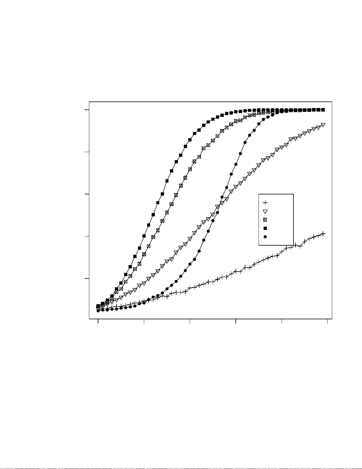
A T est for E qualit y of Distr ibution s in High Dimension s W olfga ng A. Ro lke a a Dep a rtment of Math ematics, University of Puerto Ric o - Mayag¨ uez, Mayag¨ uez, PR 00681, USA, Postal A ddr ess: PO Box 3486 , Mayag¨ uez, PR 00681, T el: (787) 255-1793, Email: wolfgang@puerto-ric o.net Angel M. L´ op ez b b Dep artment of Physics, University of Puerto Ric o - Mayag¨ uez, M ayag¨ uez, P R 00681 , USA Abstract W e presen t a metho d whic h tests wh ether or not t w o d atasets (one of whic h could b e Mon te Carlo generated) might come from the same distribution. Ou r method w orks in arbitrarily high dimensions. Key wor ds: k-nearest neigh b or, Kolmog oro v-Smrin o v test, curse of dimensionalit y Preprint submitted to Elsevier Science 19 S eptem b er 2018 1 In tro duction Man y sciences to day rely hea vily on the use of Monte Carlo sim ulation. In High Energy Ph ysics (HEP) fo r example it is used in practically ev ery stage of an exp eriment fr om the design of the detectors to the final analyses . This brings up the question of the precision of t he MC sim ulation. In other w ords, ho w close are the probability distributions of the MC to those of the exp eri- men t al da t a ? T esting whether t w o da t asets come from the same distribution is a classical problem in Sta tistics, and for one-dimensional dat a sets a larg e n um b er of methods ha v e b een dev elop ed. T es ts in higher dimensions ha v e b een prop osed by Bic k el [1] a nd F riedman and Rafsky [2] . Zec h [3] discussed a test based on the concept of minim um energy . The test prop osed here b elongs to a class of consisten t, asymptotically distribution fr ee tests based on nearest neigh b ors (Narsky [4], Bic k el and Breiman [5], Henze [6], and Sc hilling [7] ). W e concen trate in this pap er on comparing tw o dat asets, either b oth real data or one real and o ne Mon te Carlo, but the prop osed metho d also allow s us to test whether a dataset comes f r om a known theoretical distribution as long as w e can sim ulate data from this distribution. 2 2 The Metho d T o set the stage, let’s say w e hav e observ ations (ev en ts) X 1 , .., X n from some distribution F , and observ ations Y 1 , .., Y m from some distribution G . In the application we hav e in mind one of these w ould b e MC generated da t a and the other ”real” data, but this is not crucial fo r the fo llo wing. W e a re inte rested in testing H 0 : F = G vs H a : F 6 = G . The idea of our test is this: let’s c oncen trate on one of the X observ ations, say X j . What is its nearest neigh b or, that is, the observ ation closest to it ? If the n ull hy p ot hesis is correct and b oth datasets w ere generated b y the same probabilit y distribution, then this nearest neighbor is equally likely to b e one of the X or Y observ ations (prop ortional to n a nd m ). If F 6 = G there should b e regions in space where there a re relatively more X or Y observ ations than could b e expected otherwise. More formally , let Z j = 1 if the nearest neigh b or of X j is from the X data and 0 otherwise. Then, under the n ull hy p ot hesis, Z j is a Bernoulli r a ndom v ariable with succes s probabilit y ( n − 1) / ( n + m − 1). Therefore Z = P n j =1 Z j has a n appro ximate binomial distribution with parameters n and ( n − 1) / ( n + m − 1). The distribution is only approx imately bino mia l b ecause the Z ′ j s are not indep enden t, but f o r datasets of an y reasonable size the dep endence is v ery slight and can b e ignored. There is an immediate g eneralization of the test: instead o f j ust considering the nearest neigh b or we can find the k-nearest neigh b ors. No w Z j = ( Z j 1 , .., Z j k ) 3 with Z j i = 1 if the i th nearest neigh b or of X j is from the X dataset, 0 other- wise. Under the n ull h yp othesis Z = P n j =1 P k i =1 Z j i has aga in an approx imate binomial distribution with parameters nk a nd ( n − 1) / ( n + m − 1). (Actually , P k i =1 Z j i has a hy p ergeometric distribution, but b ecause we will use a k m uc h smaller than n or m the difference is negligible.) W e can find the p- v alue of the test with p = P ( V ≥ Z ) where V ∼ B in ( nk, ( n − 1) / ( n + m − 1)). Esp ecially if n and m are small or if a relativ ely la rge k is desired it w ould b e p ossible to use a p erm utatio n t yp e method to estimate the n ull distribution. The idea is as fo llo ws: under H 0 all the ev en ts come from the same distribu- tion, so an y permutation of the ev en ts will a gain ha ve the same distribution. Therefore if w e join the X and Y ev ents together, sh uffle them around and then split them again in to n a nd m ev en ts X ′ and Y ′ , these are now guaran- teed to ha v e the same distribution. Applying the k-nearest neighbor test and rep eating the ab ov e ma ny times ( say 1000 times) will give us an estimate of the null distribution. F o r more on the idea of p erm utation tests, see G o o d [8 ]. This metho d will ac hiev e the correct t yp e I error probability by construction, but it also requires a muc h greater computational effort. There are a n um b er of choices to b e made when using this metho d. First o f all, there is the question of whic h dataset should b e our X data. Clearly , if n = m , 4 this do es not matter but it migh t well otherwise. Indeed, in our application of comparing MC data t o r eal data, we hav e control o f the size of t he MC data although sometimes there ar e computational limits o n its size. Next we need to decide on k . Again there is no ob viously optimal choice here. Finally , w e need to decide on a metric to use when finding the nearest neighbor. If the o bserv atio ns differ greatly in ”size” in differen t dimensions, the standard Euclidean metric cannot b e expected to w ork w ell b ecause small differences in dimensions with a large spread would ov erwhelm small but significan t differ- ences in dimensions with a small spread. This last issue w e will deal with by standardizing eac h dimension separately , using the mean and standard devia- tion of the combine d X and Y dat a. If the da t a come f rom a distribution that is sev erely sk ewe d, ot her measures of lo catio n and spread (suc h as the median and the interquartile rang e) could also b e used to standa r dize the data . In the next section we will show the results of some mini MC studies which giv e some guidelines for the c hoices. 3 P erformance of this Method If w e use the binomial appro ximation in our test, w e will need to v erify that the metho d works , that is, that it ac hiev es the desired t yp e I error probabilit y α . Of course, we are also in terested in the pow er of the test, that is, the probabilit y to reject the null h yp ot hesis if indeed F 6 = G . In this sec tion w e 5 will carry out sev eral mini MC studies to in v estigate these questions. W e start with the situation whe re there exist o ther methods for this test, namely in one dimension. F or comparison w e will use a metho d that is kno wn to ha v e generally very go o d p o we r, t he Kolmogoro v-Smirnov (KS) test. In the first sim ulation w e generate n = m observ ations from 1000 to 20 000 in steps of 1000 each for X and Y from the uniform distribution on [0 , 1]. Because o f the probabilit y inte gral transform this is actually a v ery general case, and similar conclusions will hold fo r all ot her con tin uous distributions in one dimension. F or eac h of these cases we use our test with k = 1 , 2 , 5 , 10 , 20 , 50 a nd 100 as w ell as the KS t est. This is rep eated 1 0 000 times. Figure 1 shows the results, using a nominal t yp e I error probabilit y of α = 5%. As w e see the true t yp e I error probabilit y is close to nominal but increases slo wly as k increases. This is due to the lac k of indep endence b etw een t he Z j ’s. Esp ecially if k is larg e relativ e to n or m , the true ty p e I error probabilit y is larger than what is acceptable. Based on this and similar sim ulation studies, w e recommend k = 10 if b ot h n and m are at least 1000, otherwise k = 0 . 01 min( n, m ). Alternativ ely , one can use the p erm utation metho d describ ed ab ov e which will ha v e the correct t yp e I error b y construction. Ev en for k = 1 w e hav e a sligh tly higher than nominal t yp e I error probabilit y , ab out 5 . 5% if α = 5%. This is partly due to the dep endence b et w een the Z j ’s, and partly to the discrete nature of the bino mia l distribution. F or example, 6 if w e defined the p-v alue as P ( V ≥ Z − 1) w e w ould get a t r ue t yp e I error probabilit y sligh tly smaller than the nominal one. In an y case, w e b eliev e this difference to b e acceptable. Next a sim ulation to study the p o wer of t he test, ag a in in one dimension. W e use the uniform on [0 , 1 ] distribution for F and the uniform on [0 , θ ] for G , where θ go es from 1 to 1 . 1 W e generate n = m = 1 000 ev en ts and a pply our test with k = 1, 5, 15 and 25 as w ell as the KS test. This is rep eated 10000 times. The result is sho wn in Figure 2. Clearly , the higher the k the b etter the p ow er of the test. In fact, f o r this example already with k = 15 the test has b etter p ow er than the KS test! G enerally sp eaking, in one dimension, our test has pow er somewhat inferior to the KS test. Ho w ev er, our test is not meant to b e used in one dimension. It is encouraging to find that it do es fairly w ell ev en in that situation. Ho w should one c ho ose the size of the Monte Carlo data set r elat ive to the size of the true data? In the next simulation w e g enerate n = 100 0 ev en ts from a uniform [0 , 1] and a ssume this to b e the real data. Then we generate m ev en ts from the same distribution, with m going from 50 to 2 500. In Figure 3 w e sho w the results which indicate that the MC data set should hav e the same size as the real data b ecause in that case the true type I erro r probability is ab o ut the same as the nominal one. This agrees with general statistical exp erience whic h suggests that, in t w o-sample problems, equal sample sizes are often preferable. 7 Finally w e presen t a m ulti- dimensional example. W e generate n = m = 10 00 ev ents. The F distribution is a m ultiv ariate standard normal in 9 dimensions, and the G distribution a mu ltiv aria te normal in 9 dimensions with means 0, standard deviations 1 and cor r elat io n co efficien ts cor ( X i , X j ) = ρ if | i − j | = 1 and 0 if | i − j | > 1, where ρ go es from 0 to 0 . 5. This example illus trates the need for a test in higher dimensions. Here all the marginals are standard normals, and an y one-dimension-at-a-t ime method is certain t o miss the dif- ference b etw een F and G . This is shown in Figure 4 where with k = 10 we reject the n ull hypothesis quite easily (at ρ = 0 . 5) whereas the KS test a pplied at any of t he marginals fails completely . 4 Implemen tation A C++ routine that carries out the test is av a ilable from one o f the authors at h ttp://math.uprm.edu/˜wrolk e/ . It allows the use of the binomial approx- imation as w ell as the p erm utation metho d. It uses a simple searc h for the k-nearest neigh b ors. k-NN searc hing is a we ll kno wn problem in computer science, and more sophisticated and faster routines exist and could also b e used in combin ation with our co de. (See, f or example, F riedman, Bask ett a nd Sh ustek [9] .) 8 5 Summary W e describ e a test for t he equalit y of distributions of tw o datasets in higher dimensions. The test is conceptually simple and do es not suffer from the curse of dimensionalit y . Sim ulation studies show that it approx imately ac hiev es t he desired t yp e I error probabilit y , or do es so exactly at a higher computational cost. They also sho w that this test is capable to detect differences b et w een the distributions only ” visible” in higher dimensions. References [1] Bic k el, P . J. (1969). A distribution fr ee v ersion of the Smirnov t w o-sample test in the multiv ariate case. Annals of Mathematical Statistics 40 1-2 3 . [2] F riedman, J. H. a nd Raf sky , L. C. (1979). Multiv a r ia te generalizations o f the W ald-W olfowitz and Smirno v t wo-sample t ests. Annals o f Statistics 7(4) 69 7 -717. [3] Zec h, G. and Aslan, B. A Multiv ariate Tw o-Sa mple T est Based o n the Concept of Minimum Energy , Pro ceedings of Ph ystat200 3, SLA C, Stan- ford. [4] Narsky , Ily a (1993) Estimation of Go o dness-of-Fit in Multidime n- sional Analysis Us ing Distance to Nearest Neighbor, Ph ystat2003, arXiv:ph ysics/0306171v1 [ph ysics.data-an] [5] Bic k el, P . J. and Breiman, L. (1983). Sums of functions of nearest neigh- 9 b or distances, momen t b ounds, limit t heorems and a go o dness of fit test. Annals of Probabilit y 11 185-2 1 4. [6] Henze , N. (1988). A m ultiv ariate tw o-sample test based o n the nu mber of nearest neigh b o r coincidences. Annals of Statistics 16 772-783 . [7] Sc hilling, M. F. (198 6). Multiv ariate t wo-sample tests based on nearest neigh b ors. Journal of the American Statistical Asso ciatio n 81 799-806 . [8] Phillip G o o d, (2000 ) Pe rmutation T ests: A Practical Guide to Resampling Metho ds fo r T esting Hyp otheses, Springer V erla g . [9] F riedman, J.H., Bask ett F. and Shustek L.J.(1975) An Algorithm for Find- ing Nearest Neigh b ors. IEEE T ransactions on Computers 24, 10 0 0-1006 6 App endix 10 0 5000 10000 15000 20000 4 5 6 7 8 9 Sample Size Type I error probability (in %) 1 2 5 10 20 50 100 KS Fig. 1. The true t yp e I error probabilit y in a one dimensional example as a fun ction of sample size. X and Y ha v e a uniform distrib ution on [0 , 1]. n = m , an d the nominal type I err or probabilit y is 5%. Eac h curve represent s a different k v alue. The KS test giv es a flat lin e at 5%. 11 1.00 1.02 1.04 1.06 1.08 1.10 0.2 0.4 0.6 0.8 1.0 θ Power k=1 k=5 k=15 k=25 KS Fig. 2. F = U [0 , 1], G = U [0 , θ ] where θ goes from 1 to 1 . 1 W e generate n = m = 1000 ev en ts. k = 1, 5, 15 and 25. 12 0 500 1000 1500 2000 2500 2 4 6 8 10 m Type I error probability (in %) k=1 k=5 k=15 k=25 KS Fig. 3. n = 1000 from F = U [0 , 1], m go es from 50 to 2500, G = F . 13 0.0 0.1 0.2 0.3 0.4 0.5 0 20 40 60 80 100 ρ P ower Fig. 4. n = m = 1000. The F distribution is a m ultiv ariate standard n orm al in 9 di- mensions, and the G distribu tion a multiv ariate normal in 9 dimensions with means 0, standard deviations 1 and correlation co efficient s cor ( X i , X j ) = ρ if | i − j | = 1 and 0 if | i − j | > 1, where ρ go es from 0 to 0 . 5. Th e m ultidimensional test has m uc h b etter p o w er than an y of the one-dimensional KS tests. 14