The Weibull-Geometric distribution

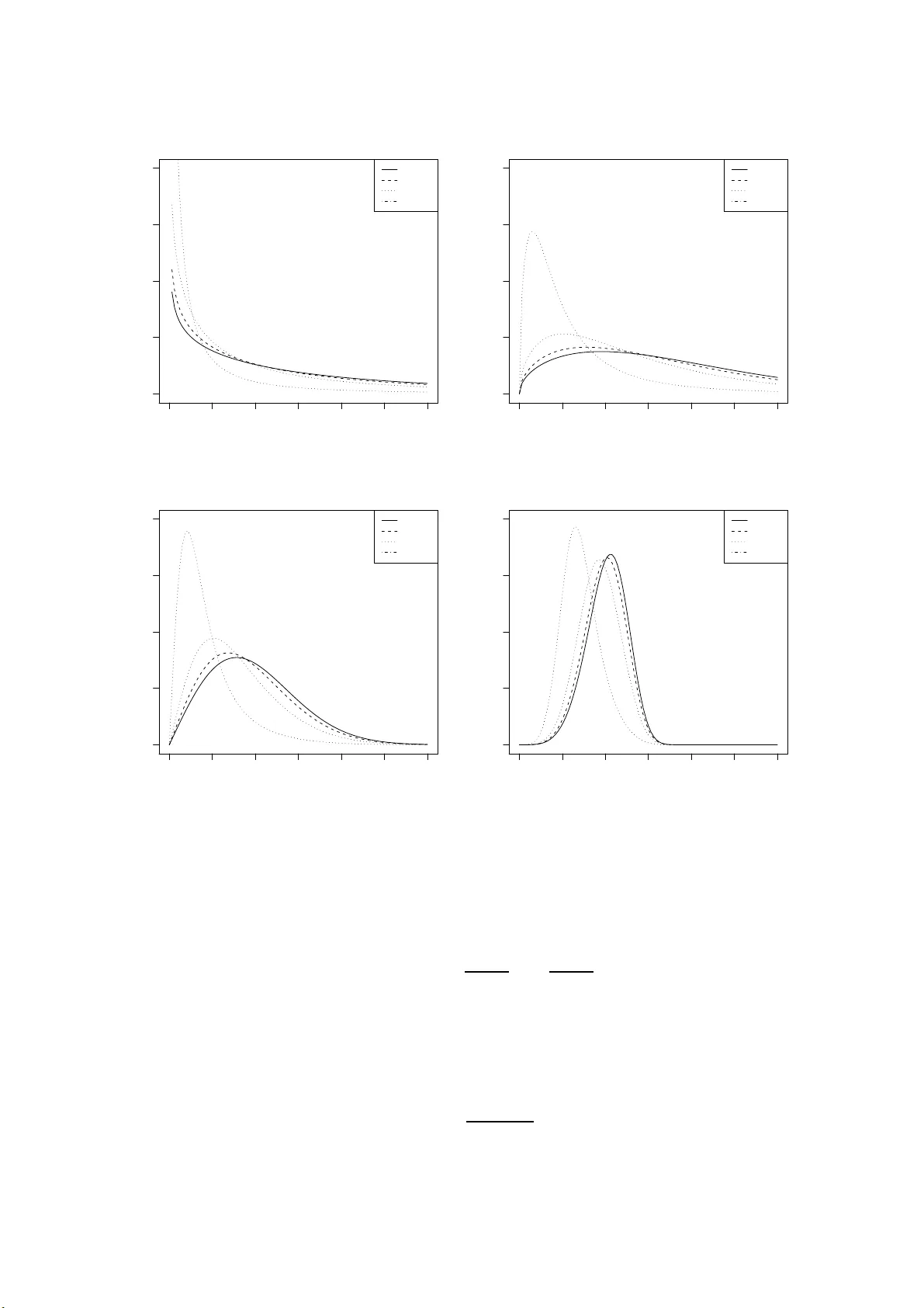
The W eibull-Geometric Distribution W agner Barreto -Souza a , Alice Lemos de Morais a and Gauss M. Cordeiro b a Departamento de Estat ´ ıstica, Univ ersidade F edera l de P ernam buco, Cidade Univ ersit´ aria, 5074 0-540 – Recife, PE, Brazi l (e-mail : w agnerbs85@hot mail. com, alice.l m@hotma i l.com) b Departamento de Estat ´ ıstica e Infor m´ atica, Univ ersidade F edera l Rural de Pernam buco, Rua Dom Mano el de Medeiros s/n, 50171-90 0 – Reci f e, PE, Brazil (e-mail : gausscordeir o@uol.co m.br) Abstract In this pap er w e i n tro d uce, for the first time, the W eibull-Geome tric distrib ution whic h generali zes the exp onenti al-geo metric distribution prop osed b y Adamidis and Louk as (1998 ). T he hazard function of th e last distribution is monotone decreasing but the hazard function of the new distribu tion can tak e more general f orms. Un lik e the W eibull distribution, the prop osed distribution is useful for mo deling unimo d al failure rates. W e deriv e the cumula tiv e distribution and hazard functions, the den- sit y of the order statistics and calculate expressions for its moments and for the momen ts of the order sta tistics. W e giv e expr essions for the R ´ en yi and Shan n on en tropies. The maxim um lik eli ho o d estimation pr o cedure is discussed and an algo- rithm EM (Dempster et al., 1977; McLac h lan and Krishnan, 1997) is provided for estimating the parameters. W e obtain the inf orm ation matrix and d iscuss inference. Applications to real data sets are giv en to sho w the flexibilit y and p oten ti alit y of the prop osed distribution. k eywords : EM algorithm; E xp onen tial distribution; Geometric d istribution; Hazard function; In formation matrix; Maxim um lik eliho o d estimatio n; W eibull dis- tribution 1 In tro duction Sev eral distributions hav e b een prop osed in the literature to mo del lifetime data. Adamidis and Louk as (1998) in t r o duced the t w o- par a meter exponentia l- geometric (EG) distribu- tion with decreasing f a ilure rat e. Kus (2007) in tro duced the exp onen tial-P oisson distri- bution (follo wing the same idea of the EG distribution) with decreasing failure rate and 1 discuss ed v a r io us o f its prop erties. Marshall and Olkin (1997) presen ted a metho d for adding a parameter to a family o f distributions with application to the exp onen tial and W eibull families. Adamidis et al. (2005) pro p osed the extended exp onen tial-geometric (EEG) distribution whic h generalizes the EG distribution and discus sed v arious of its statistical prop erties along with its reliabilit y features. The hazard function of the EEG distribution can b e monotone decreasing, increasing or constan t. The W eibull distribution is one of the most commonly used lifetime distribution in mo deling lifetime data. In practic e, it has b een shown to b e v ery flexible in mo deling v arious t yp es of lifetime distributions with monotone failure rates but it is not useful for modeling the bathtub shap ed and the unimo dal failure rates whic h are common in reliabilit y and biological studies. In this pap er we in tro duce a W eibull-geometric (W G) distribution whic h generalizes the EG and W eibul l distributions and study some of its prop erties. The pap er is org a nized as follow s. In Section 2 , w e define the W G distribution and plot its probabilit y densit y function (p df ). In Section 3, we giv e some prop erties of the new distribution. W e obtain the c um ulativ e distribution function (cdf ), surviv or and hazard functions and the p df of the order statistics. W e also giv e expressions for its momen ts and for the momen ts of the order statistics. The estimation b y maxim um lik eliho o d using the algorithm EM is studied in Section 4 and inference is disc ussed in Section 5. Illustrativ e examples based on real data are give n in Section 6 . Finally , Section 7 concludes the pap er. 2 The W G distribu tion The EG distribution (Adamidis and Louk as, 1998 ) can b e obtained by comp ounding an expo nen tial with a geometric distribution. In fact, if X follo ws a n exp onen tial distribution with para meter β Z , where Z is a g eometric v ariable with parameter p , then X has the EG distribution with parameters ( β , p ). Since the W eibull distribution generalizes the expo nen tial distribution, it is natural to extend the EG distribution b y replacing in the ab o v e comp ounding mec hanism the exp onen tial b y the W eibull distribution. Supp ose that { Y i } Z i =1 are indep enden t and iden tically dis tributed (iid) random v ari- ables follow ing the W eibull distribution W ( β , α ) with scale parameter β > 0, shap e parameter α > 0 a nd p df g ( x ; β , α ) = α β α x α − 1 e − ( β x ) α , x > 0 , and N a discrete random v ariable ha ving a geometric distribution with probabilit y func- tion P ( n ; p ) = (1 − p ) p n − 1 for n ∈ N and p ∈ (0 , 1). Let X = min { Y i } N i =1 . The marginal p df o f X is f ( x ; p, β , α ) = αβ α (1 − p ) x α − 1 e − ( β x ) α { 1 − p e − ( β x ) α } − 2 , x > 0 , (1) whic h defines the WG distribution. It is eviden t that (1) is muc h more flexible than the W eibull distribution. The EG distribution is a sp ecial case of the W G distribution for α = 1 . When p approac hes zero, the WG distribution leads to the W eibull W ( β , α ) distribution. Figure 1 plots the W G densit y for some v alues of t he v ector φ = ( β , α ) when p = 0 . 01 , 0 . 2 , 0 . 5 , 0 . 9. F or all v alues of parameters, the densit y tends to zero a s x → ∞ . 2 0.0 0.5 1.0 1.5 2.0 2.5 3.0 0.0 0.5 1.0 1.5 2.0 φ =(0.5,0.8) x f ( x ) p=0.01 p=0.2 p=0.5 p=0.9 0.0 0.5 1.0 1.5 2.0 2.5 3.0 0.0 0.5 1.0 1.5 2.0 φ =(0.5,1.5) x f ( x ) p=0.01 p=0.2 p=0.5 p=0.9 0.0 0.5 1.0 1.5 2.0 2.5 3.0 0.0 0.5 1.0 1.5 2.0 φ =(0.9,2) x f ( x ) p=0.01 p=0.2 p=0.5 p=0.9 0.0 0.5 1.0 1.5 2.0 2.5 3.0 0.0 0.5 1.0 1.5 2.0 φ =(0.9,5) x f ( x ) p=0.01 p=0.2 p=0.5 p=0.9 Figure 1: Pdf of the WG distribution for selec ted v alues of the parameters. F or α > 1, the W G densit y is unimo dal (see app endix A) and the mo de x 0 = β − 1 u 1 /α 0 is o btained by solving the nonlinear equation u 0 + pe − u 0  u 0 + α − 1 α  = α − 1 α . (2) The p df of the W G dis tribution can b e express ed as an infinite mixture of W eibull dis- tributions with the same shap e parameter α . If | z | < 1 and k > 0, w e hav e t he series represen ta tio n (1 − z ) − k = ∞ X j = 0 Γ( k + j ) Γ( k ) j ! z j . (3) 3 Expanding { 1 − p e − ( β x ) α } − 2 as in (3), w e can write (1) as f ( x ; p, β , α ) = αβ α (1 − p ) x α − 1 e − ( β x ) α ∞ X j = 0 ( j + 1) p j e − j ( β x ) α . F rom the W eibull p df giv en b efor e, w e ha v e f ( x ; p, β , α ) = (1 − p ) ∞ X j = 0 p j g ( x ; β ( j + 1) 1 /α , α ) . (4) Hence, some mathematical prop erties (cdf, momen ts, p ercen tiles, momen t generating function, fa ctorial momen ts, etc.) of the WG distribution can b e obtained using (4) from the corresponding prop erties of the W eibull distribution. 3 Prop e rties of the W G distrib ution 3.1 The distribution and hazard functions and order statistics Let X b e a random v ariable suc h that X follo ws the W G distribution with parameters p , β and α . In the sequel, the distribution of X will b e referred to W G ( p, β , α ). The cdf is g iv en b y F ( x ) = 1 − e − ( β x ) α 1 − p e − ( β x ) α , x > 0 . (5) The surviv or and hazard functions are S ( x ) = (1 − p ) e − ( β x ) α 1 − p e − ( β x ) α , x > 0 (6) and h ( x ) = αβ α x α − 1 { 1 − p e − ( β x ) α } − 1 , x > 0 , (7) respectiv ely . The hazard function (7) is decreasing for 0 < α ≤ 1. Ho w ev er, for α > 1 it can tak e differen t forms. As the W G distribution conv erges to the W eibull distribution when p → 0 + , the hazard function for v ery small v alues o f p can b e decreasing, increasing and almost constan t. When p → 1 − , the W G distribution con ve rges to a distribution degen- erate in zero. Hence , the parameter p can b e interprete d as a concen tration parameter. Figure 2 illustrates some of the p o ssible shap es of the hazard function for selec ted v alues of the ve ctor φ = ( β , α ) when p = 0 . 01 , 0 . 2 , 0 . 5 and 0 . 9. These plots sho w that the hazard function of the new distribution is quite flexible. 4 0.0 0.5 1.0 1.5 2.0 2.5 3.0 0.0 0.5 1.0 1.5 2.0 φ =(0.5,0.8) x h ( x ) p=0.01 p=0.2 p=0.5 p=0.9 0.0 0.5 1.0 1.5 2.0 2.5 3.0 0.0 0.5 1.0 1.5 2.0 φ =(0.5,1.5) x h ( x ) p=0.01 p=0.2 p=0.5 p=0.9 0.0 0.5 1.0 1.5 2.0 2.5 3.0 0 1 2 3 4 φ =(0.9,2) x h ( x ) p=0.01 p=0.2 p=0.5 p=0.9 0.0 0.5 1.0 1.5 0 2 4 6 8 10 φ =(0.9,5) x h ( x ) p=0.01 p=0.2 p=0.5 p=0.9 Figure 2: Hazard rate function of the WG distribution for selected v alues of the param- eters. W e no w calculate the p df of the order statistics. Let X 1 , . . . , X n b e random v ariables iid suc h that X i ∼ W G ( p, β , α ) for i = 1 , . . . , n . The p df of the i th order statistic, X i : n sa y , is g iv en b y (for x > 0) f i : n ( x ) = αβ α (1 − p ) n − i +1 B ( i, n − i + 1) x α − 1 e − ( n − i +1)( β x ) α { 1 − e − ( β x ) α } i − 1 { 1 − pe − ( β x ) α } n +1 , (8) where B ( a, b ) = R ∞ 0 ω a − 1 (1 − ω ) b − 1 dω denotes the b eta function. Let g i : n ( x ) b e the p df of t he i th W eibu ll order statistic with parameters β a nd α giv en b y g i : n ( x ) = αβ α B ( i, n − i + 1) x α − 1 e − ( n − i +1)( β x ) α { 1 − e − ( β x ) α } i − 1 . 5 Equation (8 ) can b e rewritten in terms of g i : n ( x ) as f i : n ( x ) = (1 − p ) n − i +1 { 1 − pe − ( β x ) α } − ( n +1) g i : n ( x ) . F urther, we can express the p df of X i : n as a mixture of W eibull order statistic densities . Using (3 ) in (8), w e obtain f i : n ( x ) = (1 − p ) n − i +1 n !( n + j − i )! ( n + j )!( n − i )! ∞ X j = 0  n + j n  p j g i : n + j ( x ) . (9) Hence, using (9), some mathematical prop erties fo r the order statistics of the W G dis- tribution can b e immediate ly o btained fro m the corresponding prop erties of the W eibull order statistics . 3.2 Quan tiles and momen ts The quan tile γ ( x γ ) of the W G distribution follow s f rom (5) as x γ = β − 1  log  1 − p γ 1 − γ  1 /α . In particular, the median is simply x 0 . 5 = β − 1 { log(1 − p ) } 1 /α . The r th momen t of X is giv en b y E ( X r ) = αβ α (1 − p ) Z ∞ 0 x r + α − 1 e − ( β x ) α  1 − p e − ( β x ) α  − 2 dx. Expanding the term { 1 − p e − ( β x ) α } − 2 as in (3) yields E ( X r ) = (1 − p )Γ( r /α + 1) p β r L ( p ; r /α ) , where L ( p ; a ) = P ∞ j = 1 p j j − a is Euler’s p olylogarithm function (see , Erdely i et al., 1953, p. 31) whic h is readily a v ailable in standard softw a re suc h as Mathematica. Figure 3 plots the sk ewness and kurtosis of the WG distribution as functions of p for β = 1 and some v alues of α . When p → 1 − , the co efficien ts of sk ewness and kurtosis tend to zero as exp ected, since the WG distribution con v erges to a degenerate distribution (in zero) when p → 1 − . The r th momen t of the i th order statistic X i : n is g iv en b y E ( X r i : n ) = αβ α (1 − p ) n − i +1 B ( i, n − i + 1) Z ∞ 0 x α + r − 1 e − ( n − i +1)( β x ) α { 1 − e − ( β x ) α } i − 1 { 1 − pe − ( β x ) α } n +1 dx. Expanding the term { 1 − pe − ( β x ) α } − ( n +1) as in (3) and using the binomial expansion for { 1 − e − ( β x ) α } i − 1 , the r th momen t of X i : n b ecomes E ( X r i : n ) = (1 − p ) n − i +1 Γ( r /α + 1) B ( i, n − i + 1) β r ∞ X j = 0 i − 1 X k =0 ( − 1) k  n + j n  i − 1 k  p j ( n + j + k − i + 1) r /α +1 . (10) 6 0.0 0.2 0.4 0.6 0.8 1.0 0.00 0.05 0.10 0.15 0.20 0.25 p skewness α =1.5 α =1.6 α =1.7 α =1.8 0.0 0.2 0.4 0.6 0.8 1.0 0.00 0.05 0.10 0.15 0.20 0.25 0.30 p kurtosis α =1.5 α =1.6 α =1.7 α =1.8 Figure 3: Sk ewness and kurtosis of the W G distribution as functions o f p for β = 1 and some v alues of α . W e now giv e an alternativ e express ion to (10) b y using a result due to Barak a t and Ab delk ader (2004) . W e ha v e E ( X r i : n ) = r n X k = n − i +1 ( − 1) k − n + i − 1  k − 1 n − i  n k  Z ∞ 0 x r − 1 S ( x ) k dx, where S ( x ) is the surviv or function (6). Using the expans ion (3) and c hanging v ariables u = ( k + j )( β x ) α , w e ha v e Z ∞ 0 x r − 1 S ( x ) k dx = (1 − p ) k ∞ X j = 0  k + j − 1 k − 1  p j Z ∞ 0 x r − 1 e − ( k + j )( β x ) α dx = (1 − p ) k αβ r Z ∞ 0 u r /α − 1 e − u du ∞ X j = 0  k + j − 1 k − 1  p j ( k + j ) r /α = (1 − p ) k Γ( r /α ) αβ r ∞ X j = 0  k + j − 1 k − 1  p j ( k + j ) r /α . Hence, E ( X r i : n ) = Γ( r /α + 1) ( − 1) n − i +1 β r ∞ X j = 0 n X k = n − i +1 ( − 1) k  n k  k − 1 n − i  k + j − 1 k − 1  p j (1 − p ) k ( k + j ) r /α . (11) Express ions (10) and (11) give the moments of the order statistics and can b e compared n umerically . T able 1 giv es nume rical v alues for the first four momen ts of the or der 7 statistics X 1:15 , X 7:15 and X 15:15 from (10) a nd (11) with the index j stopping at 1 00 and b y n umerical in tegration. W e take the parameter v alues as p = 0 . 8, β = 0 . 4 and α = 2. The figures in this table show go o d agreemen t among t he three methods. X i :15 ↓ r th momen t → r = 1 r = 2 r = 3 r = 4 Express ion (10) 0.25717 0.08697 0.035116 0.016265 i = 1 Express ion (11) 0.25717 0.08697 0.03 5116 0.0162 6 5 Numerical 0.2610 2 0.087 95 0.03 5408 0.01636 4 Express ion (10) 0.96660 0.98827 1.06643 1.21249 i = 7 Express ion (11) 0.98502 0.99295 1.06784 1.21298 Numerical 0.96674 0.98836 1.06649 1.21253 Express ion (10) 3.33109 11.97872 46.35371 19 2.32090 i = 15 Express ion (11) 3.33126 11.97875 46.35375 19 2.32090 Numerical 3.3312 6 11.97875 46.35375 192.32 0 90 T able 1: First fo ur moments of some order statistics from (10) and (11) and by n umerical in tegration. 3.3 R ´ en yi and Shannon en tropies En tropy has b een used in v arious situations in scienc e and engineering. The en trop y of a random v ariable X is a measure of v ariation of the uncertaint y . R ´ en yi en trop y is defined b y I R ( γ ) = 1 1 − γ log { R R f γ ( x ) dx } , where γ > 0 and γ 6 = 1 . By using (3), we hav e Z ∞ 0 f γ ( x ; p, β , α ) dx = [ αβ α (1 − p )] γ Γ(2 γ ) ∞ X j = 0 p j Γ(2 γ + j ) j ! Z ∞ 0 x ( α − 1) γ e − ( γ + j )( β x ) α dx. If ( α − 1)( γ − 1 ) ≥ 0, this expression reduces to Z ∞ 0 f γ ( x ; p, β , α ) dx = Γ( α )[ α (1 − p )] γ β α (1 − γ ) Γ(2 γ ) ∞ X j = 0 p j Γ(2 γ + j ) j !( α + j ) E ( Y ( α − 1)( γ − 1) j ) , where Y j follo ws a gamma distribution with scale parameter ( γ + j ) 1 /α and shap e param- eter α . Hence, w e obtain I R ( γ ) = 1 1 − γ log ( [ α (1 − p )] γ Γ( γ ( α − 1) + 1 ) β 1 − γ Γ(2 γ ) ∞ X j = 0 p j Γ(2 γ + j ) j !( α + j ) ( α − 1)( γ − 1) /α +1 ) . Shannon en trop y is defined as E {− log[ f ( X )] } . This is a sp ecial case obtained from lim γ → 1 I R ( γ ). Then, E [ − log f ( X )] = − log[ α β α (1 − p )] − ( α − 1) E [log ( X )] + β α E ( X α ) − 2 E { log [1 − pe − ( β X ) α ] } . 8 W e can sho w that E [log ( X )] = ψ (1) /α, E ( X α ) = − (1 − p ) pβ α log(1 − p ) , E { log [1 − pe − ( β X ) α ] } = − 1 − p p { 1 + (1 − p )[1 + log (1 − p )] } . Hence, the Shannon en tropy reduces to E [ − log f ( X )] = − log[ α β α (1 − p )] − α − 1 α ψ (1) − 1 − p p [4 − 2 p + (3 − 2 p ) log(1 − p )] . 4 Estimation Let x = ( x 1 , . . . , x n ) b e a random sample of the W G distribution with unkno wn parameter v ector θ = ( p, β , α ). The log lik eliho o d ℓ = ℓ ( θ ; x ) for θ is ℓ = n [log α + α log β + log (1 − p )] + ( α − 1) n X i =1 log( x i ) − n X i =1 ( β x i ) α − 2 n X i =1 log[1 − p e − ( β x i ) α ] . The score function U ( θ ) = ( ∂ ℓ/∂ p, ∂ ℓ/∂ β , ∂ ℓ/∂ α ) T has components ∂ ℓ ∂ p = − n (1 − p ) − 1 + 2 n X i =1 e − ( β x i ) α [1 − p e − ( β x i ) α ] − 1 , ∂ ℓ ∂ β = nα β − 1 − α β α − 1 n X i =1 x α i { 1 + 2 p e − ( β x i ) α [1 − p e − ( β x i ) α ] − 1 } , ∂ ℓ ∂ α = nα − 1 + n X i =1 log( β x i ) − n X i =1 ( β x i ) α log( β x i ) { 1 + 2 p e − ( β x i ) α [1 − p e − ( β x i ) α ] − 1 } . The maxim um lik eliho o d estimate (MLE) b θ of θ is calculated n umerically from the nonlinear equations U ( θ ) = 0. W e use the EM algorithm (Dempster et a l., 19 7 7; McLac h- lan and Krishnan, 1997) to obtain b θ . F or doing this, w e define an hypothetical complete- data distribution with densit y function f ( x, z ; θ ) = α β α (1 − p ) z x α − 1 p z − 1 e − z ( β x ) α , for x, β , α > 0, p ∈ (0 , 1) and z ∈ N . Under this form ulation, the E-step of an EM cycle require s the conditional expectation of ( Z | X ; θ ( r ) ), where θ ( r ) = ( p ( r ) , β ( r ) , α ( r ) ) is the curren t estimate o f θ . Using that P ( z | x ; θ ) = z p z − 1 e − ( z − 1)( β x ) α × { 1 − pe − ( β x ) α } 2 for z ∈ N , it fo llo ws E ( Z | X ; θ ) = { 1 + pe − ( β x ) α }{ 1 − pe − ( β x ) α } − 1 . The EM cycle is completed with the M-step b y using the maxim um like liho o d estimation ov er θ , with the missing Z ’s 9 replaced b y their conditional exp ectations giv en ab ov e. Hence , an EM iteration reduces to p ( r +1) = 1 − n P n i =1 w ( r ) i , β ( r +1) = n ( n X i =1 x α ( r +1) i w ( r ) i ) − 1 /α ( r +1) , where α ( r +1) is t he solution of the nonlinear equation n α ( r +1) + n X i =1 log x i − n P n i =1 w ( r ) i x α ( r +1) i log x i P n i =1 w ( r ) i x α ( r +1) i = 0 , where w ( r ) i = 1 + p ( r ) e − ( β ( r ) x i ) α ( r ) 1 − p ( r ) e − ( β ( r ) x i ) α ( r ) . An impleme n tation o f this algorithm using the soft w are R is giv en in Appendix B. 5 Inference F or interv al estimation and hy p othesis tests on the mo del parameters, we require the information matrix. The 3 × 3 observ ed information matrix J n = J n ( θ ) is giv en b y J n =   J pp J pβ J pα J pβ J β β J β α J pα J β α J αα   , where − J pp = ∂ 2 ℓ ∂ p 2 = 2 n X i =1 T ( i ) 0 , 0 , 2 , 2 − n (1 − p ) − 2 , − J pα = ∂ 2 ℓ ∂ p ∂ α = − 2 β α n X i =1 ( p T ( i ) 1 , 1 , 2 , 2 + T ( i ) 1 , 1 , 1 , 1 ) , − J pβ = ∂ 2 ℓ ∂ p ∂ β = − 2 αβ α − 1 n X i =1 ( p T ( i ) 1 , 0 , 2 , 2 + T ( i ) 1 , 0 , 1 , 1 ) , − J αα = ∂ 2 ℓ ∂ α 2 = − nα − 2 + n X i =1 (2 p 2 β 2 α T ( i ) 2 , 2 , 2 , 2 + 2 pβ 2 α T ( i ) 2 , 2 , 1 , 1 − β α T ( i ) 1 , 2 , 0 , 0 − 2 pβ α T ( i ) 1 , 2 , 1 , 1 ) , − J β α = ∂ 2 ℓ ∂ α ∂ β = nβ − 1 − β α − 1 n X i =1 ( αT ( i ) 1 , 1 , 0 , 0 + T ( i ) 1 , 0 , 0 , 0 )(1 + 2 pT ( i ) 0 , 0 , 1 , 1 ) + 2 pαβ 2 α − 1 n X i =1 ( p T ( i ) 2 , 1 , 2 , 2 + T ( i ) 2 , 1 , 1 , 1 ) , 10 − J β β = ∂ 2 ℓ ∂ β 2 = − nαβ − 2 − α ( α − 1) β α − 2 n X i =1 ( T ( i ) 1 , 0 , 0 , 0 + 2 pT ( i ) 1 , 0 , 1 , 1 ) + 2 α 2 β 2 α − 2 p n X i =1 ( pT ( i ) 2 , 0 , 2 , 2 + T ( i ) 2 , 0 , 1 , 1 ) . Here, T ( i ) j,k ,l, m = T ( i ) j,k ,l, m ( x i , θ ) = x αj i { log( β x i ) } k { 1 − p e − ( β x i ) α } − l e − m ( β x i ) α , for ( j, k , l , m ) ∈ { 0 , 1 , 2 } and i = 1 , . . . , n . Under conditions that a re fulfilled for the parameter θ in the inte rior of the parameter space but not on the b oundary , the asymp- totic distribution of √ n ( b θ − θ ) is multiv ariate normal N 3 (0 , K ( θ ) − 1 ), whe re K ( θ ) = lim n →∞ n − 1 J n ( θ ) is the unit informatio n matrix. This asymptotic b ehav ior remains v alid if K ( θ ) is replaced b y the a v erage sample information matrix ev aluated at b θ , i.e., n − 1 J n ( b θ ). W e can use the asymptotic m ultiv ariate normal N 3 (0 , J n ( b θ ) − 1 ) distribution of b θ to cons- truct a ppro ximate confidence regions for some parameters and fo r the hazard and surviv al functions. In fact, an 10 0 (1 − γ )% a symptotic confidence inte rv al for each parameter θ i is g iv en b y AC I i = ( b θ i − z γ / 2 p b J θ i θ i , b θ i + z γ / 2 p b J θ i θ i ) , where b J θ i θ i represen ts t he ( i, i ) diagonal elemen t of J n ( b θ ) − 1 for i = 1 , 2 , 3 , 4 a nd z γ / 2 is the quan tile 1 − γ / 2 of the standard normal distribution. The asymptotic normalit y is also useful for testing go o dness of fit of the three param- eter W G distribution and f o r comparing this distribution with some of its sp ecial sub- mo dels via the likel iho o d ratio (LR) statistic. W e consid er the par titio n θ = ( θ T 1 , θ T 2 ) T , where θ 1 is a subset of parameters of intere st o f the WG distribution and θ 2 is a subset of the remaining parameters. The LR statistic for testing the n ull h yp othesis H 0 : θ 1 = θ (0) 1 v ersus the alternativ e h yp othesis H 1 : θ 1 6 = θ (0) 1 is giv en by w = 2 { ℓ ( ˆ θ ) − ℓ ( ˜ θ ) } , where ˜ θ and b θ denote the MLEs under the n ull and a lternative h yp otheses, resp ectiv ely . The statistic w is asymptotically (as n → ∞ ) distributed as χ 2 k , where k is the dimension of the subset θ 1 of intere st. F or example, w e can compare the EG model against the W G mo del b y t esting H 0 : α = 1 vers us H 1 : α 6 = 1 and the W eib ull mo del against the W G mo del b y testing H 0 : α = 1 , p = 0 v ersus H 1 : H 0 is f alse. 6 Applications In this section, we fit the W G mo dels to t wo real data sets. The first data set consist of the num b er of successiv e failures fo r the air conditioning system o f eac h mem b er in a fleet of 13 Bo eing 720 jet airplanes. The p o oled data with 214 observ ations w ere first analyzed b y Prosc han (1963) and discussed further b y Dahiy a and Gurland (1972), G leser (1989), Adamidis and Louk as (1998) and K us (2007). The second data set is an uncensored data set fr o m Nic ho ls a nd P adgett (2006) consisting of 100 observ ations on breaking stress o f carb on fibres (in Gba). 11 F or the first data set, the estimated parameters using an EM algorithm w ere ˆ p = 0 . 7841, ˆ β = 0 . 0 0 48 and ˆ α = 1 . 22 4 6. The fitted p df and the estimated quan tiles v ersus observ ed quan tiles are give n in Figures 4. This figure sho ws a go o d fit of the W G mo del for the first data set. Densidade 0 100 200 300 400 500 600 0.000 0.002 0.004 0.006 0.008 0.010 0 100 200 300 400 500 600 0 200 400 600 800 1000 1200 1400 Quantil Empírico Quantil Teórico − WG Figure 4: Plots of the fitted p df and of the estimated quan tiles v ersus observ ed quantile s for the first data set. F or the second data set, the estimates obtained using an EM algorithm are ˆ p = 0 . 3073, ˆ β = 0 . 3148 and ˆ α = 3 . 0 0 93. The plot of the fitted p df and the estimated quan tiles ve rsus observ ed quan tiles in F ig ure 5 sho ws a go o d fit of the W G mo del. 7 Conclus i o ns W e define a new mo del so called the W eibull-geometric (WG) distribution that generalizes the exp onen tial-g eometric (EG) distribution introduced b y Adamidis and Louk as (19 9 8). Some mathematical prop erties are deriv ed a nd plots of the p df and hazard functions are presen ted to sho w the flexibilit y of the new distribution. W e giv e closed form expres sions for the momen ts of the distribution. W e obtain the p df of the order statistics and pro vide expansions for the momen ts of the order statistics. Estimation b y maxim um lik eliho o d is discussed and an a lg o rithm EM is prop osed. W e discuss inference, giv e asymptotic confidence in terv als f o r the mo del parameters and presen t the use of the LR statistic to compare the fit of the WG mo del with sp ecial sub-mo dels. Finally , w e fitted W G mo dels to tw o real data sets to sho w the flexibilit y and the p oten tially of t he new distribution. 12 Densidade 0 1 2 3 4 5 6 0.0 0.1 0.2 0.3 0.4 0.5 1 2 3 4 5 0 1 2 3 4 5 6 7 Quantil Empírico Quantil Teórico − WG Figure 5: Plots of the fitted p df and of the estimated quan tiles v ersus observ ed quantile s for the second data set. App endix A W e now sho w that the W G densit y is unimo dal when α > 1. L et h ( u ) = u + pe − u  u + α − 1 α  . When u → 0 + , h ( u ) → p α − 1 α and when u → ∞ , h ( u ) → ∞ . Th us, if h ( u ) is an increasing function, the solution in (2) is uniqu e and the W G distribution is unimo dal. W e hav e h ′ ( u ) = 1 − pe − u  u + α − 1 α  + pe − u . Using the inequalities − pe − u α − 1 α > − pe − u and − pe − u u > e − 1, it follows that h ′ ( u ) > 1 − e − 1 > 0, ∀ u > 0. Hence , h ( u ) is an increasing function and the W G distribution is unimodal if α > 1. App endix B The following R function estimates the mo del para meters p , β a nd α through an EM algorithm. fit.WG<- function (x,par,t ol=1e-4,maxi=100){ # x Numerica l vector of data. # par Vector of initial values for the parameter s p, beta and a lpha # to be optimized over, on this exactly order. # tol Convergenc e tolerance . 13 #maxi Upper end point of the interval to be searched. p<-par[1 ] beta<-pa r[2] alpha<-p ar[3] n<-lengt h(x) z.temp<- function (){ (1+p*exp (-(beta* x)^alpha ))/(1-p*exp(-(beta*x)^alpha)) } alpha.sc <-functi on(alpha ){ n/alpha+ sum(log( x))-n*su m(z*x^alpha*log(x))/sum(z*x^al pha) } test<-1 while(te st>tol){ z<-z.tem p() alpha.ne w<-(alph a.sc,int erval=c(0,maxi))$root beta.new <-(n/sum (x^alpha .new*z))^(1/alpha.new) p.new<-1 -n/sum(z ) test<-ma x(abs(c( ((alpha. new-alpha)), ((beta.n ew-beta) ), ((p.new- p))))) alpha<-a lpha.new beta<-be ta.new p<-p.new } c(p,beta ,alpha) } References [1] Adamidis K, D imitrak op oulou, T, Louk as S (2005) On a g eneraliz ation of the expo nen tial-geometric distribution. Statist. and Probab. Lett., 7 3:259-269 [2] Adamidis K, Louk a s S (199 8) A lifetime distribution with decreasing failure rate. Statist. and Probab. Lett., 39:35-42 [3] Barak at HM, Ab delk ader YH (2004) Computing the moments of order statistics from noniden tical random v ariables. Statistical Methods and Applications, 1 3 :15-26 [4] Dahiy a R C, Gurland J (1972 ) Go o dness of fit tests for the gamma and exp onential distributions. T ec hnometrics, 14 :791-801 [5] Dempster AP , Laird NM, Rubim DB (1977 ) Maxim um lik eliho o d from incomplete data via the EM algorithm (with discussion). J. Roy . Statist. So c. Ser. B, 39:1-38 [6] Erdelyi A, Magnus W, Ob erhettinger F, T ricomi FG (1953 ) Hi gher T ranscenden tal F unctions . McGra w-Hill, New Y o rk 14 [7] Gleser LJ (1989) The g amma distribution a s a mixture of exponential distributions. Amer. Statist., 43:115- 117 [8] Kus C (2007) A new lifetime distribution. Computat. Statist. Data Analysis, 51:4497- 4509 [9] Nic hols MD, P adgett WJ (2006). A bo otstrap con trol c hart for W eibull p ercen tiles. Qualit y and Reliabilit y Engineering In ternational, 22:141-1 5 1 [10] Marshall A W, O lkin I (1997) A new metho d for a dding a parameter to a family of distributions with application to the exp onenti al and W eibu ll families. Biometrik a, 84:641-652 [11] McLac hlan GJ, Krishnan T (1997) The EM Algorithm and Extension. Wiley , New Y ork [12] Prosc han (1963) Theoretical explanation of o bserv ed decre asing failure rate. T echno- metrics, 5:375-383 15