Large Scale Variational Inference and Experimental Design for Sparse Generalized Linear Models

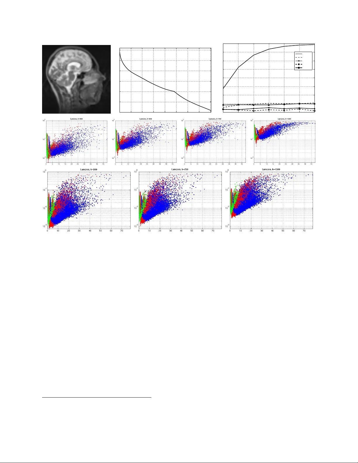
Large Scale V ariational Inference and Exp erimen tal Design for Sparse Generalized Linear Mo dels Matthias W. Seeger ∗ Hannes Nic kisch † Octob er 22, 2018 Abstract Man y problems of low-lev el computer vision and image pro cessing, suc h as denoising, de- con volution, tomographic reconstruction or super-resolution, can b e addressed b y maximizing the p osterior distribution of a sparse linear model (SLM). W e sho w how higher-order Ba yesian decision-making problems, suc h as optimizing image acquisition in magnetic resonance scanners, can be addressed b y querying the SLM posterior co v ariance, unrelated to the densit y’s mode. W e prop ose a scalable algorithmic framework, with which SLM p osteriors o ver full, high-resolution images can b e approximated for the ﬁrst time, solving a v ariational optimization problem which is con vex iﬀ posterior mo de ﬁnding is con vex. These methods successfully driv e the optimization of sampling tra jectories for real-w orld magnetic resonance imaging through Ba yesian experimen- tal design, which has not been attempted before. Our metho dology provides new insigh t into similarities and diﬀerences b etw een sparse reconstruction and appro ximate Bay esian inference, and has imp ortan t implications for compressiv e sensing of real-world images. Parts of this work app eared at conferences [33, 22]. 1 In tro duction Natural images ha ve a sparse lo w-lev el statistical signature, represented in the prior distribution of a sparse linear model (SLM). Imaging problems suc h as reconstruction, denoising or decon volu- tion can successfully b e solved by maximizing its p osterior density (maxim um a p osteriori (MAP) estimation), a conv ex program for certain SLMs, for whic h eﬃcien t solv ers are a v ailable. The suc- cess of these techniques in modern imaging practice has somewhat shrouded their limited scop e as Bay esian tec hniques: of all the information in the posterior distribution, they make use of the densit y’s mode only . Consider the problem of optimizing image ac quisition , our ma jor motiv ation in this work. Mag- netic resonance images are reconstructed from F ourier samples. With scan time prop ortional to the num b er of samples, a central question to ask is which sampling designs of minimum size still lead to MAP reconstructions of diagnostically useful image qualit y? This is not a direct recon- struction problem, the fo cus is on improving measuremen t designs to b etter supp ort subsequent ∗ Saarland Univ ersity and Max Planc k Institute for Informatics, Campus E1.4, 66123 Saarbr ¨ uc ken, German y ( mseeger@mmci.uni-saarland.de ). † Max Planc k Institute for Biological Cyb ernetics, Sp emannstraße 38, 72076 T¨ ubingen, Germany ( hn@tuebingen.mpg.de ). 1 reconstruction. Goal-directed acquisition optimization cannot sensibly b e addressed b y MAP es- timation, y et w e show how to successfully driv e it b y Ba yesian p osterior information b eyond the mo de. Adv anced decision-making of this kind needs uncertain t y quan tiﬁcation (posterior co v ari- ance) rather than p oint estimation, requiring us to step out of the sp arse r e c onstruction scenario and approximate sp arse Bayesian infer enc e instead. The Bay esian inference relaxation w e fo cus on is not new [11, 23, 17], yet when it comes to problem c haracterization or eﬃcien t algorithms, previous inference work lags far behind standards estab- lished for MAP reconstruction. Our contributions range from theoretical c haracterizations o v er no vel scalable solv ers to applications not previously attempted. The inference relaxation is sho wn to b e a conv ex optimization problem if and only if this holds for MAP estimation (Section 3), a prop ert y not previously established for this or any other SLM inference appro ximation. More- o ver, we develop nov el sc alable double lo op algorithms to solve the v ariational problem orders of magnitude faster than previous metho ds w e are a w are of (Section 4). These algorithms exp ose an imp ortan t link betw een v ariational Ba yesian inference and sparse MAP reconstruction, reducing the former to calling v arian ts of the latter few times, interlea v ed by Gaussian co v ariance (or PCA) appro ximations (Section 4.4). By wa y of this reduction, the massive recen t interest in MAP estima- tion can play a role for v ariational Bay esian inference just as well. T o complement these similarities and clarify confusion in the literature, w e discuss computational and statistical diﬀerences of sparse estimation and Ba yesian inference in detail (Section 5). The ultimate motiv ation for no vel dev elopments presen ted here is sequen tial Ba yesian experimental design (Section 6), applied to acquisition optimization for medical imaging. W e present a p o werful v ariant of adaptiv e compressive sensing, which succeeds on real-world image data where theoretical prop osals for non-adaptive compressive sensing [9, 6, 10] fail (Section 6.1). Among our experimental results is part of a ﬁrst successful study for Bay esian sampling optimization of magnetic resonance imaging, learned and ev aluated on real-world image data (Section 7.4). An implementation of the algorithms presented here is publicly a v ailable, as part of the glm-ie to olbox (Section 4.6). It can b e downloaded from mloss.org/software/view/269/ . 2 Sparse Ba y esian Inference. V ariational Appro ximations In a sparse linear model (SLM), the image u ∈ R n of n pixels is unknown, and m linear measure- men ts y ∈ R m are given, where m  n in many situations of practical interest. y = X u + ε , ε ∼ N ( 0 , σ 2 I ) , (1) where X ∈ R m × n is the design matrix , and ε is Gaussian noise of v ariance σ 2 , implying the Gaussian lik eliho o d P ( y | u ) = N ( y | X u , σ 2 I ). Natural images are characterized b y histograms of simple ﬁlter resp onses (deriv ativ es, w a velet co eﬃcien ts) exhibiting sup er-Gaussian (or sp arse ) form: most coeﬃcients are close to zero, while a small fraction hav e signiﬁcan t sizes [35, 28] (a precise deﬁnition of sup er-Gaussianit y is giv en in Section 2.1). Accordingly , SLMs hav e sup er- Gaussian prior distributions P ( u ). The MAP estimator ˆ u MAP := argmax u [log P ( y | u ) + log P ( u )] can outp erform maximum lik eliho o d ˆ u ML := argmax u log P ( y | u ), when u represen ts an image. In this pap er, w e fo cus on priors of the form P ( u ) ∝ Q q i =1 t i ( s i ), where s = B u . The p oten tial functions t i ( · ) are p ositiv e and b ounded. The op erator B ∈ R q × n ma y contain deriv ative ﬁlters or a 2 w av elet transform. Both X and B hav e to b e structured or sparse, in order for an y SLM algorithm to b e scalable. L aplac e (or double exp onen tial) p oten tials are sparsity-enforcing: t i ( s i ) = e − τ i | s i | , τ i > 0 . (2) F or this particular prior and the Gaussian lik eliho od (1), MAP estimation corresponds to a quadratic program, known as LASSO [37] for B = I . Note that log t i ( s i ) is concav e. In gen- eral, if lo g-c onc avity holds for all mo del p oten tials, MAP estimation is a conv ex problem. Another example for sparsit y p oten tials are Student’s t : t i ( s i ) = (1 + ( τ i /ν ) s 2 i ) − ( ν +1) / 2 , τ i , ν > 0 . (3) F or these, log t i ( s i ) is not conca ve, and MAP estimation is not (in general) a conv ex program. Note that − log t i ( s i ) is also known as Lorentzian p enalt y function. 2.1 V ariational Lo w er Bounds Ba yesian inference amounts to computing momen ts of the p osterior distribution P ( u | y ) = Z − 1 N ( y | X u , σ 2 I ) Y q i =1 t i ( s i ) , s = B u , Z = Z N ( y | X u , σ 2 I ) Y q i =1 t i ( s i ) d u . (4) This is not analytically tractable in general for sparse linear mo dels, due to tw o reasons coming together: P ( u | y ) is highly coupled ( X is not blo ckdiagonal) and non-Gaussian. W e fo cus on vari- ational appro ximations here, rooted in statistical ph ysics. The lo g p artition function log Z (also kno wn as log evidence or log marginal lik eliho o d) is the prime target for v ariational metho ds [42]. F ormally , the p oten tials t i ( s i ) are replaced by Gaussian terms of parametrized width, the p osterior P ( u | y ) b y a Gaussian approximation Q ( u | y ). The width parameters are adjusted by ﬁtting Q ( u | y ) to P ( u | y ), in what amoun ts to the v ariational optimization problem. ← γ → 0 2 4 6 8 0 2 4 6 8 h( γ ) ← γ → 0 2 4 6 8 1.4 1.6 1.8 2 h( γ ) ← γ → 0 2 4 6 8 0 1 2 3 4 h( γ ) Figure 1: Sup er-Gaussian distributions admit tigh t Gaussian-form low er b ounds of an y width γ . Left: Laplace (2); middle: Bernoulli (6); right: Student’s t (3). 3 Our v ariational relaxation exploits the fact that all p oten tials t i ( s i ) are (str ongly) sup er-Gaussian : there exists a b i ∈ R such that ˜ g i ( s i ) := log t i ( s i ) − b i s i is ev en, and conv ex and decreasing as a function of x i := s 2 i [23]. W e write g i ( x i ) := ˜ g i ( x 1 / 2 i ), x i ≥ 0 in the sequel. This implies that t i ( s i ) = max γ i ≥ 0 e b i s i − s 2 i / (2 γ i ) − h i ( γ i ) / 2 , h i ( γ i ) := max x i ≥ 0 ( − x i /γ i − 2 g i ( x i )) . (5) A sup er-Gaussian t i ( s i ) has tight Gaussian-form lo wer bounds of all widths (see Figure 1). W e replace t i ( s i ) b y these low er b ounds in order to step from P ( u | y ) to the family of appro ximations Q ( u | y ) ∝ P ( y | u ) e b T s − 1 2 s T (diag γ ) − 1 s , where γ = ( γ i ). T o establish (5), note that the extended-v alue function g i ( x i ) (assigning g i ( x i ) = ∞ for x i < 0) is a closed prop er conv ex function, th us can b e represen ted b y F enchel dualit y [26, Sect. 12]: g i ( x i ) = sup λ i x i λ i − g ∗ i ( λ i ), where the conjugate function g ∗ i ( λ i ) = sup x i x i λ i − g i ( x i ) is closed con vex as well. F or x i ≥ 0 and λ i > 0, we hav e that x i λ i − g i ( x i ) ≥ x i λ i − g i (0) → ∞ with x i → ∞ , whic h implies that g ∗ i ( λ i ) = ∞ for λ i > 0. Also, g ∗ i (0) = − lim x i →∞ g i ( x i ), so that − g ∗ i (0) < g i ( x i ) for an y x i < ∞ . Therefore, for any x i ∈ [0 , ∞ ), g i ( x i ) = sup λ i < 0 x i λ i − g ∗ i ( λ i ). Reparameterizing γ i := − 1 / (2 λ i ), w e ha ve that g i ( x i ) = max γ i ≥ 0 − x i / (2 γ i ) − g ∗ i ( − 1 / (2 γ i )) (note that in order to accommo date g i (0) in general, we hav e to allo w for γ i = 0). Finally , h i ( γ i ) := 2 g ∗ i ( − 1 / (2 γ i )). The class of super-Gaussian p oten tials is large. All scale mixtures (mixtures of zero-mean Gaussians t i ( s i ) = E γ i [ N ( s i | 0 , γ i )]) are sup er-Gaussian, and h i ( γ i ) can b e written in terms of the density for γ i [23]. Both Laplace (2) and Studen t’s t p oten tials (3) are super-Gaussian, with h i ( γ i ) given in App endix A.6. Bernoulli p oten tials, used as binary classiﬁcation likelihoo ds, t i ( s i ) =  1 + e − y i τ i s i  − 1 , y i ∈ {± 1 } , τ i > 0 (6) are sup er-Gaussian, with b i = y i τ i / 2 [17, Sect. 3.B]. While the corresp onding h i ( γ i ) cannot be determined analytically , this is not required in our algorithms, which can be implemen ted based on g i ( x i ) and its deriv ativ es only . Finally , if the t ( l ) i ( s i ) are sup er-Gaussian, so is the p ositiv e mixture P L l =1 α l t ( l ) i ( s i ), α l > 0, b ecause the lo gsumexp function x 7→ log 1 T exp( x ) [4, Sect. 3.1.5] is strictly conv ex on R L and increasing in each argument, and the log-mixture is the concatenation of lo gsumexp with (log t ( l ) i ( s i ) + log α l ) l , the latter conv ex and decreasing for x i = s 2 i > 0 in each comp onen t [4, Sect. 3.2.4]. A natural criterion for ﬁtting Q ( u | y ) to P ( u | y ) is obtained b y plugging these b ounds in to the partition function Z of (4): Z ≥ e − h ( γ ) / 2 Z N ( y | X u , σ 2 I ) e b T s − 1 2 s T Γ − 1 s d u , h ( γ ) := X q i =1 h i ( γ i ) , (7) where Γ := diag γ and s = B u . The right hand side is a Gaussian integral and can b e ev aluated easily . The v ariational problem is to maximize this low er b ound w.r.t. the v ariational parameters γ  0 ( γ i ≥ 0 for all i = 1 , . . . , q ), with the aim of tightening the appro ximation to log Z . This criterion can b e interpreted as a divergence function: if the family of all Q ( u | y ) contained the true p osterior P ( u | y ), the latter would maximize the b ound. This relaxation has frequently b een used b efore [11, 23, 17] on inference problems of mo derate size. In the following, w e pro vide results that extend its sc ope to large scale imaging problems of interest here. In the next section, w e characterize the conv exity of the underlying optimization problem precisely . In Section 4, w e provide a new class of algorithms for solving this problem orders of magnitude faster than previously used techniques. 4 3 Con v exit y Prop erties of V ariational Inference In this section, we c haracterize the v ariational optimization problem of maximizing the right hand side of (7). W e show that it is a conv ex problem if and only if all p oten tials t i ( s i ) are log-conca ve, whic h is equiv alen t to MAP estimation b eing conv ex for the same mo del. W e start b y conv erting the low er b ound (7) into a more amenable form. The Gaussian posterior Q ( u | y ) has the cov ariance matrix Co v Q [ u | y ] = A − 1 , A := σ − 2 X T X + B T Γ − 1 B , Γ = diag γ . (8) W e hav e that Z P ( y | u ) e b T s − 1 2 s T Γ − 1 s d u = | 2 π A − 1 | 1 / 2 max u P ( y | u ) e b T s − 1 2 s T Γ − 1 s , s = B u , since max u Q ( u | y ) = | 2 π A − 1 | − 1 / 2 R Q ( u | y ) d u . W e ﬁnd that Z ≥ C 1 e − φ ( γ ) / 2 , where φ ( γ ) := log | A | + h ( γ ) + min u R ( u , γ ) , R := σ − 2 k y − X u k 2 + s T Γ − 1 s − 2 b T s (9) and C 1 = (2 π ) ( n − m ) / 2 σ − m . The v ariational problem is min γ  0 φ ( γ ), and the Gaussian posterior appro ximation is Q ( u | y ) with the ﬁnal parameters γ plugged in. W e will also write φ ( u , γ ) := log | A | + h ( γ ) + R ( u , γ ), so that φ ( γ ) = min u φ ( u , γ ). It is instructive to compare this v ariational inference problem with maximum a p osteriori (MAP) estimation: min u − 2 log P ( u | y ) = min u σ − 2 k y − X u k 2 − 2 X i log t i ( s i ) + C 2 = min u , γ  0 h ( γ ) + R ( u , γ ) + C 2 , (10) where C 2 is a constant. The diﬀerence b et ween these problems rests on the log | A | term, presen t in φ ( γ ) y et absen t in MAP . Ultimately , this observ ation is the key to the characterization provided in this section and to the scalable solvers developed in the subsequen t section. Its full relev ance will b e clariﬁed in Section 5. 3.1 Con v exity Results In this section, w e pro ve that φ ( γ ) is conv ex if all potentials t i ( s i ) are log-conca ve, with this condition b eing necessary in general. W e address each term in (9) separately . Theorem 1 L et X ∈ R m × n , B ∈ R q × n b e arbitr ary matric es, and ˜ A ( d ) := σ − 2 X T X + B T (diag d ) B , d  0 , so that ˜ A ( d ) is p ositive deﬁnite for al l d  0 . (1) L et f i ( γ i ) b e twic e c ontinuously diﬀer entiable functions into R + , so that log f i ( γ i ) ar e c onvex for al l i and γ i . Then, γ 7→ log | ˜ A ( f ( γ )) | is c onvex. Esp e cial ly, γ 7→ log | A | is c onvex. 5 (2) L et f i ( π i ) b e c onc ave functions into R + . Then, π 7→ log | ˜ A ( f ( π )) | is c onc ave. Esp e cial ly, γ − 1 7→ log | A | is c onc ave. (3) L et f i ( γ i ) b e c onc ave functions into R + . Then, γ 7→ 1 T (log f ( γ )) + log | ˜ A ( f ( γ ) − 1 ) | is c onc ave. Esp e cial ly, γ 7→ 1 T (log γ ) + log | A | is c onc ave. (4) L et Q ( u | y ) b e the appr oximate p osterior with c ovarianc e matrix given by (8). Then, for al l i : V ar Q [ s i | y ] = δ T i B A − 1 B T δ i ≤ γ i . A proof is provided in App endix A.1. Instantiating part (1) with f i ( γ i ) = γ − 1 i , w e see that γ 7→ log | A | is conv ex. Other v alid examples are f i ( γ i ) = γ − β i i , β i > 0. F or f i ( γ i ) = e γ i , we obtain the con vexit y of γ 7→ log | ˜ A (exp( γ )) | , generalizing the lo gsumexp function to matrix v alues. P art (2) and part (3) will b e required in Section 4.2. Finally , part (4) gives a precise characterization of γ i as sparsity parameter, regulating the v ariance of s i . Theorem 2 The function γ 7→ φ ( γ ) − h ( γ ) = log | A | + min u  σ − 2 k y − X u k 2 + s T Γ − 1 s − 2 b T s  is c onvex for γ  0 , wher e s = B u . Pr o of . The con v exity of log | A | has b een sho wn in Theorem 1(1). σ − 2 k y − X u k 2 − 2 b T s is con vex in u , and ( u , γ ) 7→ s T Γ − 1 s is jointly con v ex, since the quadratic-o ver-linear function ( s i , γ i ) 7→ s 2 i /γ i is join tly conv ex for γ i > 0 [4, Sect. 3.1.5]. Therefore, min u R ( u , γ ) is conv ex for γ  0 [4, Sect. 3.2.5]. This completes the pro of. T o put this result into context, note that φ ( γ ) − h ( γ ) = − 2 log Z P ( y | u ) e b T s − 1 2 s T Γ − 1 s d u , s = B u is the ne gative log partition function of a Gaussian with natural parameters γ − 1 : it is well known that γ − 1 7→ φ ( γ ) − h ( γ ) is a c onc ave function [42]. How ev er, γ − 1 7→ h ( γ ) is c onvex for a mo del with sup er-Gaussian potentials (recall that h i ( γ i ) = 2 g ∗ i ( − 1 / (2 γ i )), where g ∗ i ( · ) is con vex as dual function of g i ( · )), whic h means that in general γ − 1 7→ φ ( γ ) need not b e con vex or conca ve. The c onvexity of this negative log partition function w.r.t. γ seems sp eciﬁc to the Gaussian case. Giv en Theorem 2, if all h i ( γ i ) are conv ex, the whole v ariational problem min γ  0 φ is conv ex. With the following theorem, we characterize this case precisely . Theorem 3 Consider a mo del with Gaussian likeliho o d (1) and a prior P ( u ) ∝ Q q i =1 t i ( s i ) , s = B u , so that al l t i ( s i ) ar e str ongly sup er-Gaussian, me aning that ˜ g i ( s i ) = log t i ( s i ) − b i s i is even, and g i ( x i ) = ˜ g i ( x 1 / 2 i ) is strictly c onvex and de cr e asing for x i > 0 . (1) If ˜ g i ( s i ) is c onc ave and twic e c ontinuously diﬀer entiable for s i > 0 , then h i ( γ i ) is c onvex. On the other hand, if ˜ g 00 i ( s i ) > 0 for some s i > 0 , then h i ( γ i ) is not c onvex at some γ i > 0 . (2) If al l ˜ g i ( s i ) ar e c onc ave and twic e c ontinuously diﬀer entiable for s i > 0 , then the variational pr oblem min γ  0 φ is a c onvex optimization pr oblem. On the other hand, if ˜ g 00 i ( s i ) > 0 for some i and s i > 0 , then h ( γ ) is not c onvex, and ther e exist some X , B , and y such that φ ( γ ) is not a c onvex function. 6 The pro of is giv en in Appendix A.2. Our theorem provides a complete c haracterization of con vexit y for the v ariational inference relaxation of Section 2, which is the same as for MAP estimation. Log- conca vity of all p oten tials is suﬃcient, and necessary in general, for the conv exit y of either. W e are not a ware of a comparable equiv alence ha ving been established for an y other non trivial appro ximate inference metho d for contin uous v ariable mo dels. W e close this section with some examples. F or Laplacians (2), h i ( γ i ) = τ 2 i γ i (see App endix A.6). F or SLMs with these p oten tials, MAP estimation is a con v ex quadratic program. Our result implies that v ariational inference is a con v ex problem as w ell, alb eit with a diﬀeren tiable criterion. Bernoulli p oten tials (6) are log-concav e. MAP estimation for generalized linear mo dels with these p oten tials is kno wn as p enalized logistic regression, a con vex problem t ypically solv ed by the iterativ ely rew eighted least squares (IRLS) algorithm. V ariational inference for this mo del is also a con vex problem, and our algorithms introduced in Section 4 make use of IRLS as well. Finally , Studen t’s t p oten tials (3) are not log-conca ve, and h i ( γ i ) is neither conv ex nor concav e (see App endix A.6). Neither MAP estimation nor v ariational inference are conv ex in this case. Con vexit y of an algorithm is desirable for man y reasons. No restarting is needed to a v oid lo cal minima. T ypically , the result is robust to small p erturbations of the data. These stability prop erties b ecome all the more imp ortan t in the con text of sequen tial exp erimental design (see Section 6), or when Bay esian model selection 1 is used. How ev er, the conv exity of φ ( γ ) do es not necessarily imply that the minim um p oint can b e found eﬃciently . In the next section, we prop ose a class of algorithms that solve the v ariational problem for v ery large instances, by decoupling the criterion (9) in a nov el wa y . 4 Scalable Inference Algorithms In this section, w e prop ose nov el algorithms for solving the v ariational inference problem min γ φ in a scalable wa y . Our algorithms can b e used whether φ ( γ ) is conv ex or not, they are guaran teed to con verge to a stationary p oin t. All eﬀorts are reduced to well known, scalable algorithms of signal reconstruction and numerical mathematics, with little extra technology required, and no additional heuristics or step size parameters to b e tuned. W e begin with the sp ecial case of log-concav e p otentials t i ( s i ), such as Laplace (2) or Bernoulli (6), extending our framework to full generality in Section 4.1. The v ariational inference problem is con vex in this case (Theorem 3). Previous algorithms for solving min γ φ ( γ ) [11, 23] are of the c o or dinate desc ent type, minimizing φ w.r.t. one γ i at a time. Unfortunately , suc h algorithms cannot b e scaled up to imaging problems of in terest here. An update of γ i dep ends on the marginal p osterior Q ( s i | y ), whose computation requires the solution of a linear system with matrix A ∈ R n × n . At the pro jected scale, neither A nor a decomp osition thereof can be main tained, systems ha ve to b e solv ed iterativ ely . Now, eac h of the q potentials has to be visited at least once, t ypically sev eral times. With q , n , and m in the h undred thousands, it is certainly infeasible to solve O ( q ) linear systems. In con trast, the algorithms we develop here often con verge after less than h undred systems hav e b een solv ed. W e could also feed φ ( γ ) and its gradient ∇ γ φ in to an oﬀ-the-shelf gradient-based optimizer. Ho wev er, as already noted in Section 3, φ ( γ ) is the sum of a standard penalized least squares (MAP) part and a highly coupled, computationally diﬃcult term. The algorithms we prop ose take accoun t of this decomp osition, decoupling the troublesome term in inner lo op standard form problems whic h 1 Mo del selection (or hyperparameter learning) is not discussed in this pap er. It can b e implemented easily by maximizing the lo wer b ound − φ ( γ ) / 2 + log C 1 ≤ log Z w.r.t. hyperparameters. 7 can b e solved b y an y of a large num b er of sp ecialized algorithms not applicable to min γ φ ( γ ). The exp ensiv e part of ∇ γ φ has to b e computed only a few times for our algorithms to conv erge. W e mak e use of a p ow erful idea kno wn as double lo op or c onc ave-c onvex algorithms. Sp ecial cases of suc h algorithms are frequently used in machine learning, computer vision, and statistics: the exp ectation-maximization (EM) algorithm [8], v ariational mean ﬁeld Bay esian inference [1], or CCCP for discrete approximate inference [48], among man y others. The idea is to tangen tially upp er b ound φ b y decoupled functions φ z whic h are m uch simpler to minimize than φ itself: algo- rithms iterate b et w een reﬁtting φ z to φ and minimizing φ z . F or example, in the EM algorithm for maximizing a log marginal lik eliho o d, these stages corresp ond to “E step” and “M step”: while the criterion could well b e minimized directly (at the exp ense of one “E step” p er criterion ev aluation), “M step” minimizations are muc h easier to do. As noted in Section 3, if the v ariational criterion (9) lack ed the log | A | part, it would corresp ond to a p enalized least squares MAP ob jectiv e (10), and simple eﬃcien t algorithms w ould apply . As discussed in Section 4.4, ev aluating log | A | or its gradient are computationally challenging. Crucially , this term satisﬁes a concavit y prop ert y . As shown in Section 4.2, F enchel duality implies that log | A | ≤ z T 1 ( γ − 1 ) − g ∗ 1 ( z 1 ). F or an y ﬁxed z 1  0 , the upp er bound is tangentially tigh t, con vex in γ , and decouples additiv ely . If log | A | is replaced b y this upp er bound, the resulting ob jectiv e φ z 1 ( u , γ ) := z T 1 ( γ − 1 ) + h ( γ ) + R ( u , γ ) − g ∗ 1 ( z 1 ) is of the same decoupled penalized least squares form than a MAP criterion (10). This decomp osition suggests a double lo op algorithm for solving min γ φ ( γ ). In inner lo op minimizations , w e solve min u , γ  0 φ z 1 for ﬁxed z 1  0 , and in interjacen t outer lo op up dates , we reﬁt z 1 ← argmin φ z 1 ( u , γ ). The MAP estimation ob jectiv e (10) and φ z 1 ( u , γ ) ha v e a similar form. Sp eciﬁcally , recall that − 2 g i ( x i ) = min γ i ≥ 0 x i /γ i + h i ( γ i ), where g i ( x i ) = ˜ g i ( x 1 / 2 i ) and ˜ g i ( s i ) = log t i ( s i ) − b i s i . The inner lo op problem is min u , γ  0 φ z 1 ( u , γ ) = min u σ − 2 k y − X u k 2 − 2 X q i =1  g i ( z 1 ,i + s 2 i ) + b i s i  , (11) where s = B u . This is a smoothed version of the MAP estimation problem, whic h w ould b e obtained for z 1 ,i = 0. How ev er, z 1 ,i > 0 in our approximate inference algorithm at all times (see Section 4.2). Upon inner lo op conv ergence to u ∗ , γ ∗ ,i = − 1 / [2( dg i /dx i ) | x i = z 1 ,i + s 2 ∗ ,i ], where s ∗ = B u ∗ . Note that in order to run the algorithm, the analytic form of h i ( γ i ) need not b e known. F or Laplace p otentials (2), the inner lo op p enalizer is 2 P i τ i q z 1 ,i + s 2 i , and γ ∗ ,i = q z 1 ,i + s 2 ∗ ,i /τ i . Imp ortan tly , the inner lo op problem (11) is of the same simple p enalized least squares form than MAP estimation, and an y of the wide range of recent eﬃcient solv ers can b e plugged into our metho d. F or example, the iter atively r eweighte d le ast squar es (IRLS) algorithm [14], a v ariant of the Newton-Raphson metho d, can b e used (details are given in Section 4.3). Each Newton step requires the solution of a linear system with a matrix of the same form as A (8), the con vergence rate of IRLS is quadratic. It follows from the deriv ation of (9) that once an inner loop has con v erged to ( u ∗ , γ ∗ ), the minimizer u ∗ is the mean of the approximate p osterior Q ( u | y ) for γ ∗ . The rationale behind our algorithms lies in de c oupling the v ariational criterion φ via a F enchel dual- it y upp er b ound, thereby matching algorithmic scheduling to the computational complexity struc- ture of φ . T o appreciate this p oin t, note that in an oﬀ-the-shelf optimizer applied to min γ  0 φ ( γ ), b oth φ ( γ ) and the gradient ∇ γ φ hav e to b e computed frequen tly . In this resp ect, the log | A | cou- pling term pro ves by far more computationally c hallenging than the rest (see Section 4.4). This ob vious computational diﬀerence b et w een parts of φ ( γ ) is not exploited in standard gradien t based 8 algorithms: they require all of ∇ γ φ in eac h iteration, all of φ ( γ ) in every single line searc h step. As discussed in Section 4.4, computing log | A | to high accuracy is not feasible for mo dels of inter- est here, and most oﬀ-the-shelf optimizers with fast con vergence rates are v ery hard to run with suc h approximately computed criteria. In our algorithm, the critical part is recognized and decou- pled, resulting inner lo op problems can b e solved b y robust and eﬃcien t standard co de, requiring a minimal eﬀort of adaptation. Only at the start of eac h outer lo op step, φ z 1 has to b e reﬁtted: z 1 ← ∇ γ − 1 log | A | (see Section 4.2), the computationally critical part of ∇ γ φ is required there. F enchel dualit y b ounding 2 is used to minimize the num b er of these costly steps (further adv antages are noted at the end of Section 4.4). Resulting double lo op algorithms are simple to implemen t based on eﬃcien t p enalized least squares reconstruction co de, taking full adv antage of the very w ell-researched state of the art for this setup. 4.1 The General Case In this section, w e generalize the double lo op algorithm along t w o directions. First, if p oten tials log t i ( s i ) are not log-concav e, the inner lo op problems (11) are not con vex in general (Theorem 3), y et a simple v ariant can b e used to remedy this defect. Second, as detailed in Section 4.2, there are diﬀeren t wa ys of decoupling log | A | , giving rise to diﬀerent algorithms. In this section, w e concen trate on dev eloping these v ariants, their practical diﬀerences and implications thereof are elab orated on in Section 5. If t i ( s i ) is not log-concav e, then h i ( γ i ) is not conv ex in general (Theorem 3). In this case, w e can write h i ( γ i ) = h ∩ ,i ( γ i ) + h ∪ ,i ( γ i ), where h ∩ ,i is concav e and nondecreasing, h ∪ ,i is conv ex. Such a decomp osition is not unique, and has to b e c hosen for each h i at hand. With hindsigh t, h ∩ ,i should b e c hosen as small as possible (for example, h ∩ ,i ≡ 0 if t i ( s i ) is log-conca ve, the case treated abov e), and if IRLS is to b e used for inner loop minimizations (see Section 4.3), h ∪ ,i should b e twice con tinuously diﬀeren tiable. F or Studen t’s t p oten tials (3), such a decomp osition is given in App endix A.6. W e deﬁne h ∩ ( γ ) = P i h ∩ ,i ( γ i ), h ∪ ( γ ) = P i h ∪ ,i ( γ i ), and mo dify outer loop up dates b y applying a second F enc hel dualit y b ounding operation: h ∩ ( γ ) ≤ ˜ z T 2 γ − ˜ g ∗ 2 ( ˜ z 2 ), resulting in a v arian t of the inner lo op criterion (11). If h ∩ ,i is diﬀerentiable, the outer lo op up date is ˜ z 2 ← h 0 ∩ ,i ( γ i ), otherwise an y elemen t from the subgradien t can be c hosen (note that ˜ z 2 ≥ 0, as h ∩ ,i is nondecreasing). Moreo ver, as shown in Section 4.2, F enc hel dualit y can b e emplo yed in order to b ound log | A | in t wo diﬀeren t wa ys, one emplo y ed ab o v e, the other b eing log | A | ≤ z T 2 γ − 1 T (log γ ) − g ∗ 2 ( z 2 ), z 2  0 . Com bining these b ounds (by adding ˜ z 2 to z 2 ), we obtain φ ( γ , u ) ≤ φ z ( u , γ ) := z T 1 ( γ − 1 ) + z T 2 γ − z T 3 (log γ ) + h ∪ ( γ ) + R ( u , γ ) − g ∗ ( z ) , where z 3 ,i ∈ { 0 , 1 } , and g ∗ ( z ) collects the oﬀsets of all F enchel duality b ounds. Note that z j  0 for j = 1 , 2 , 3, and for each i , either z 1 ,i > 0 and z 3 ,i = 0, or z 1 ,i = 0 and z 2 ,i > 0 , z 3 ,i = 1. W e hav e that φ z ( u ) := min γ  0 φ z ( u , γ ) = σ − 2 k y − X u k 2 + 2 X q i =1 h ∗ i ( s i ) − 2 b T s , h ∗ i ( s i ) := 1 2 min γ i ≥ 0 ( z 1 ,i + s 2 i ) /γ i + z 2 ,i γ i − z 3 ,i log γ i + h ∪ ,i ( γ i ) , s = B u . (12) 2 Note that F enchel dualit y b ounding is also used in diﬀerence-of-conv ex programming, a general framework to address non-con vex, typically non-smo oth optimization problems in a double lo op fashion. In our application, φ ( γ ) is smo oth in general and conv ex in many applications (see Section 3): our reasons for applying b ound minimization are diﬀeren t. 9 Note that h ∗ i ( s i ) is conv ex as minimum (ov er γ i ≥ 0) of a join tly con vex argument [4, Sect. 3.2.5]. The inner lo op minimization problem min u (min γ φ z ) is of p enalized least squares form and can b e solv ed with the same arra y of eﬃcien t algorithms applicable to the special case (11). An application of the second order IRLS metho d is detailed in Section 4.3. A schema for the full v ariational inference algorithm is giv en in Algorithm 1. Algorithm 1 Double lo op v ariational inference algorithm rep eat if ﬁrst outer lo op iteration then Initialize b ound φ z . u = 0 . else Outer lo op up date: Reﬁt upp er b ound φ z to φ (tangent at γ ). Requires marginal v ariances ˆ z = diag − 1 ( B A − 1 B T ) (Section 4.4). Initialize u = u ∗ (previous solution). end if rep eat Newton (IRLS) iteration to minimize min γ  0 φ z (12) w.r.t. u . En tails solving a linear system (by LCG) and line search (Section 4.3). un til u ∗ = argmin u (min γ  0 φ z ) conv erged Up date γ = argmin γ  0 φ z ( u ∗ , · ). un til outer lo op conv erged The algorithms are sp ecialized to the t i ( s i ) through h ∗ i ( s i ) and its deriv atives. The imp ortan t special case of log-concav e t i ( s i ) has b een detailed ab ov e. F or Student’s t p oten tials (3), a decomp osition is detailed in App endix A.6. In this case, the o verall problem min γ  0 φ ( γ ) is not conv ex, y et our double lo op algorithm iterates o v er standard-form con vex inner lo op problems. Finally , for log- conca ve t i ( s i ) and z 2 ,i 6 = 0 (type B bounding, Section 4.2), our algorithm can be implemen ted generically as detailed in App endix A.5. W e close this section establishing some characteristics of these algorithms. First, w e found it useful to initialize them with constan t z 1 and/or z 2 of small size, and with u = 0 . Moreov er, eac h subsequen t inner lo op minimization is started with u = u ∗ from the last round. The developmen t of our algorithms is inspired b y the sparse estimation metho d of [43], relationships to whic h are discussed in Section 5. Our algorithms are globally conv ergen t, a stationary p oin t of φ ( γ ) is found from any starting p oin t γ  0 (recall from Theorem 3 that for log-concav e p oten tials, this stationary p oin t is a global solution). This is seen as detailed in [43]. In tuitively , at the b eginning of eac h outer lo op iteration, φ z and φ ha v e the same tangent plane at γ , so that eac h inner lo op minimization decreases φ signiﬁcantly unless ∇ γ φ = 0 . Note that this conv ergence pro of requires that outer lo op up dates are done exactly , this p oint is elab orated on at the end of Section 4.4. Our v ariational infer enc e algorithms diﬀer from previous metho ds 3 in that orders of magnitude larger models can successfully b e addressed. They apply to the particular v ariational relaxation in tro duced in Section 3, whose relationship to other inference appro ximations is detailed in [29]. While most previous relaxations attain scalability through many factorization assumptions con- cerning the appro ximate p osterior, Q ( u | y ) in our metho d is fully coupled, sharing its conditional indep endence graph with the true p osterior P ( u | y ). A high-level view on our algorithms, discussed 3 This commen t holds for appro ximate infer enc e methods. F or sparse estimation , large scale algorithms are av ailable (see Section 5). 10 in Section 4.4, is that we replace a priori indep endence (factorization) assumptions by less damaging lo w rank approximations, tuned at runtime to the p osterior shap e. 4.2 Bounding log | A | W e need to upp er b ound log | A | by a term which is conv ex and decoupling in γ . This can b e done in tw o diﬀerent w a ys using F enc hel dualit y , giving rise to b ounds with diﬀerent c haracteristics. Details for the developmen t here are given in App endix A.4. Recall our assumption that A  0 for each γ  0 . If π = γ − 1 , then π 7→ log | ˜ A ( π ) | = log | A | is conca ve for π  0 (Theorem 1(2) with f ≡ id). Moreo ver, log | ˜ A ( π ) | is increasing and unbounded in eac h component of π (Theorem 4). F enc hel duality [26, Sect. 12] implies that log | ˜ A ( π ) | = min z 1  0 z T 1 π − g ∗ 1 ( z 1 ) for π  0 , th us log | A | = min z 1  0 z T 1 ( γ − 1 ) − g ∗ 1 ( z 1 ) for γ  0 . Therefore, log | A | ≤ z T 1 ( γ − 1 ) − g ∗ 1 ( z 1 ). F or ﬁxed γ  0 , this is an equality for z 1 , ∗ = ∇ γ − 1 log | A | = ˆ z := (V ar Q [ s i | y ]) = diag − 1  B A − 1 B T   0 , and g ∗ 1 ( z 1 , ∗ ) = z T 1 , ∗ ( γ − 1 ) − log | A | . This is called b ounding type A in the sequel. On the other hand, γ 7→ 1 T (log γ ) + log | A | is conca ve for γ  0 (Theorem 1(3) with f ≡ id). Emplo ying F enc hel duality once more, w e ha ve that log | A | ≤ z T 2 γ − 1 T (log γ ) − g ∗ 2 ( z 2 ), z 2  0 . F or an y ﬁxed γ , equality is attained at z 2 , ∗ = γ − 1 ◦ ( 1 − γ − 1 ◦ ˆ z ), and g ∗ 2 ( z 2 , ∗ ) = z T 2 , ∗ γ − log | A | − 1 T (log γ ) at this p oin t. This is referred to as b ounding type B. 0 2 4 6 8 10 0 1 2 3 4 5 Type A: z 1 T ( γ −1 ) − g 1 * (z 1 ) Type B: z 2 T γ − 1 T (log γ ) − g 2 * (z 2 ) Function: log|A| = log(1+2/ γ ) γ * Figure 2: Comparison of t yp e A and B upp er b ounds on log (1 + 2 /γ ). In general, type A b ounding is tighter for γ i a wa y from zero, while type B b ounding is tighter for γ i close to zero (see Figure 2), implications of this p oin t are discussed in Section 5. Whatever b ounding t yp e we use, reﬁtting the corresp onding upper b ound to log | A | requires the computation of ˆ z = (V ar Q [ s i | y ]): all marginal varianc es of the Gaussian distribution Q ( s | y ). In general, computing Gaussian marginal v ariances is a hard numerical problem, which is discussed in more detail in Section 4.4. 11 4.3 The Inner Lo op Optimization The inner loop minimization problem is given b y (12), its special case (11) for log-conca ve p oten tials and log | A | b ounding t yp e A is given by h ∗ i ( s i ) = − g i ( z 1 ,i + s 2 i ). This problem is of standard p enalized least squares form, and a large n um b er of recent algorithms [12, 3, 46] can be applied with little customization eﬀorts. In this section, w e pro vide details ab out how to apply the iter atively r eweighte d le ast squar es (IRLS) algorithm [14], a sp ecial case of the Newton-Raphson metho d. W e describ e a single IRLS step here, starting from u . Let r := X u − y denote the residual vector. If θ i := ( h ∗ i ) 0 ( s i ) − b i , ρ i := ( h ∗ i ) 00 ( s i ), then ∇ u ( φ z / 2) = σ − 2 X T r + B T θ , ∇∇ u ( φ z / 2) = σ − 2 X T X + B T (diag ρ ) B . Note that ρ i ≥ 0 by the conv exit y of h ∗ i . The Newton search direction is d := − ( σ − 2 X T X + B T (diag ρ ) B ) − 1 ( σ − 2 X T r + B T θ ) . The computation of d requires us to solv e a system with a matrix of the same form as A , a rew eighted least squares problem otherwise used to compute the means in a Gaussian mo del of the structure of Q ( u | y ). W e solve these systems appro ximately by the (preconditioned) line ar c onjugate gr adients (LCG) algorithm [13]. The cost p er iteration of LCG is dominated by matrix- v ector multiplications (MVMs) with X T X , B , and B T . A line search along d can b e run in negligible time. If f ( t ) := φ z ( u + t d ) / 2, then f 0 ( t ) = σ − 2 (( X d ) T r + t k X d k 2 ) + ( B d ) T θ ( t ) , where θ ( t ) is the gradien t at s ( t ) = s + t B d . With ( X d ) T r , k X d k 2 , and B d precomputed, f ( t ) and f 0 ( t ) can b e ev aluated in O ( q ) without any further MVMs. The line search is started with t 0 = 1. Finally , once u ∗ = argmin u φ z ( u ) is found, γ is explicitly up dated as argmin φ z ( u ∗ , · ). Note that at this p oin t, u ∗ = E Q [ u | y ], which follo ws from the deriv ation at the b eginning of Section 3. 4.4 Estimation of Gaussian V ariances V ariational inference do es require marginal v ariances ˆ z = diag − 1 ( B A − 1 B T ) = (V ar Q [ s i | y ]) of the Gaussian Q ( s | y ) (see Section 4.2), whic h are m uc h harder to appro ximate than means. In this section, w e discuss a general metho d for (co)v ariance appro ximation. Empirically , the p erformance of our double lo op algorithms is remark ably robust in the ligh t of substantial o v erall v ariance appro ximation errors, some insights into this ﬁnding are giv en b elo w. Marginal p osterior v ariances ha ve to b e computed in any appro ximate Bay esian inference metho d, while they are not required in t ypical sparse point estimation tec hniques (see Section 5). Our double lo op algorithms reduce approximate inference to p oin t estimation and Gaussian (co)v ariance appro ximation. Not only do they exp ose the latter as missing link b et ween sparse estimation and v ariational inference, their main rationale is that Gaussian v ariances hav e to b e computed a few times only , while oﬀ-the-shelf v ariational optimizers query them for ev ery single criterion ev aluation. Marginal v ariance approximations ha v e been proposed for sparsely connected Gaussian Marko v random ﬁelds (MRFs), iterating ov er embedded spanning tree mo dels [41] or exploiting rapid cor- relations deca y in mo dels with homogeneous prior [20]. In applications of interest here, A is neither sparse nor has useful graphical mo del structure. Committing to a lo w-rank appro ximation of the co v ariance A − 1 [20, 27], an optimal c hoice in terms of preserving v ariances is principal comp onents analysis (PCA), based on the smallest eigen v alues/-vectors of A (the largest of A − 1 ). The L anczos algorithm [13] provides a scalable appro ximation to PCA and was emplo y ed for v ariance estimation 12 in [27]. After k iterations, we ha ve an orthonormal basis Q k ∈ R n × k , within which extremal eigen- v ectors of A are rapidly w ell appro ximated (due to the nearly line ar sp ectral deca y of typical A ma- trices (Figure 6, upp er panel), b oth largest and smallest eigenv alues are obtained). As Q T k A Q k = T k is tridiagonal, the Lanczos v ariance approximation ˆ z k = diag − 1 ( B Q k T − 1 k Q T k B T ) can b e computed eﬃcien tly . Importantly , ˆ z k,i ≤ ˆ z k +1 ,i ≤ ˆ z i for all k and i . Namely , if Q k = [ q 1 . . . q k ], and T k has main diagonal ( α l ), sub diagonal ( β l ), let ( e l ) and ( d l ) b e the main and subdiagonal of the bidi- agonal Cholesky factor L k of T k . Then, d k − 1 = β k − 1 /e k − 1 , e k = ( α k − d 2 k − 1 ) 1 / 2 , with d 0 = 0. If V k := B Q k L − T k , we hav e V k = [ v 1 . . . v k ], v k = ( B q k − d k − 1 v k − 1 ) /e k . Finally , ˆ z k = ˆ z k − 1 + v 2 k (with ˆ z 0 = 0 ). Unfortunately , the Lanczos algorithm is muc h harder to run in practice than LCG, and its cost grows sup erlinearly in k . A promising v ariant of selectively reorthogonalized Lanczos [24] is given in [2], where contribu tions from undesired parts of the sp ectrum ( A ’s largest eigenv alues in our case) are ﬁltered out by replacing A with p olynomials of itself. Recently , randomized PCA approac hes hav e b ecome p opular [15], although their relev ance for v ariance approximation is unclear. Nevertheless, for large scale problems of in terest, standard Lanczos can be run for k  n iterations only , at whic h p oin t most of the ˆ z k,i are sev erely underestimated (see Section 7.3). Since Gaussian v ariances are essen tial for v ariational Bay esian inference, yet scalable, uniformly accurate v ariance estimators are not known, r obustness to v ariance approximations errors is critical for any large scale approximate inference algorithm. What do the Lanczos v ariance approximation errors imply for our double lo op algorithms? First, the global conv ergence pro of of Section 4.1 requires exact v ariances ˆ z , th us ma y b e compromised if ˆ z k is used instead. This problem is analyzed in [31]: the con vergence pro of remains v alid with the PCA approximation, which ho wev er is diﬀerent from the Lanczos 4 appro ximation. Empirically , we did not encoun ter conv ergence problems so far. Surprisingly , while ˆ z k is muc h smaller than ˆ z in practice, there is little indication of substan tial negativ e impact on performance. This imp ortan t robustness property is analyzed in Section 7.3 for an SLM with Laplace p oten tials. The underestimation bias has systematic structure (Figure 6, middle and low er panel): moderately small ˆ z i are damp ed most strongly , while large ˆ z i are ap- pro ximated accurately . This happ ens b ecause the largest coeﬃcients ˆ z i dep end most strongly on the largest cov ariance eigen vectors, which are shap ed in early Lanczos iterations. This particular error structure has statistical consequences. Recalling the inner lo op p enalty for Laplacians (2): h ∗ i ( s i ) = τ i ( ˆ z i + s 2 i ) 1 / 2 , the smaller ˆ z i , the stronger it enforces sparsity . If ˆ z i is underestimated, the p enalt y on s i is stronger than in tended, y et this strengthening do es not happ en uniformly . Co eﬃcien ts s i deemed most relev ant with exact v ariance computation (largest ˆ z i ) are least aﬀected (as ˆ z k,i ≈ ˆ z i for those), while already sub dominan t ones (smaller ˆ z i ) are suppressed even stronger (as ˆ z k,i  ˆ z i ). At least in our exp erience so far (with sparse linear mo dels), this selective v ariance underestimation eﬀect seems b enign or even somewhat b eneﬁcial. 4.5 Extension to Group Poten tials There is substantial recen t interest in methods incorporating sparse gr oup p enalization , meaning that a num b er of latent co eﬃcien ts (such as the column of a matrix, or the incoming edge weigh ts for a graph) are penalized join tly [47, 40]. Our algorithms are easily generalized to mo dels with 4 While Lanczos can b e used to compute the PCA appro ximation (ﬁxed num ber L of smallest eigenv alues/-vectors of A ), this is rather wasteful. 13 p oten tials of the form t i ( k s i k ), s i a sub vector of s , k · k the Euclidean norm, if t i ( · ) is ev en and sup er-Gaussian. Such gr oup p otentials are frequen tly used in practice. The isotropic total v ariation p enalt y is the sum of k ( dx i , dy i ) k , dx i , dy i diﬀerences along diﬀerent axes, whic h corresp onds to group Laplace p oten tials. In our MRI application (Section 7.4), we deal with complex-v alued u and s . Eac h entry is treated as elemen t in R 2 , and potentials are placed on | s i | = k ( < s i , = s i ) k . Note that with t i on k s i k , the single parameter γ i is shared b y the co eﬃcien ts s i . The generalization of our algorithms to group p oten tials is almost automatic. F or example, if all s i ha ve the same dimensionality , Γ − 1 is replaced by Γ − 1 ⊗ I in the deﬁnition of A , and ˆ z is replaced b y ( I ⊗ 1 T ) diag − 1 ( B A − 1 B T ) in Section 4.2. Moreo ver, x i = s 2 i is replaced b y x i = k s i k 2 , whereas the deﬁnition of g i ( x i ) remains the s ame. Apart from these simple replacemen ts, only IRLS inner lo op iterations hav e to b e mo diﬁed (at no extra cost), as is detailed in App endix A.7. 4.6 Publicly Av ailable Co de: The glm-ie T o olb o x Algorithms and techniques presen ted in this pap er are implemen ted 5 as part of the gener alize d line ar mo del infer enc e and estimation to olb o x ( glm-ie ), maintained as mloss.org pro ject at mloss.org/ software/view/269/ . The co de runs with b oth Matlab 7 and the free Octave 3.2 . It comprises algorithms for MAP (p enalized least squares) estimation and v ariational inference in generalized linear mo dels (Section 4), along with Lanczos co de for Gaussian v ariances (Section 4.4). Its generic design allo ws for a range of applications, as illustrated by a num b er of example programs included in the pac k age. Many sup er-Gaussian p oten tials t i ( s i ) are included, others can easily b e added by the user. In particular, the to olb o x contains a range of solv ers for MAP and inner lo op problems, from IRLS (or truncated Newton, see Section 4.3) o v er conjugate gradients to Quasi- Newton, as w ell as a range of commonly used op erators to construct X and B matrices. 5 Sparse Estimation and Sparse Ba y esian Inference In this section, we con trast appro ximate Bay esian inference with p oin t estimation for sparse linear mo dels (SLMs): sp arse Bayesian infer enc e v ersus sp arse estimation . These problem classes serv e distinct goals and come with diﬀerent algorithmic c haracteristics, y et are frequen tly confused in the literature. Brieﬂy , the goal in sparse estimation is to eliminate v ariables not needed for the task at hand, while sparse inference aims at quantifying uncertaint y in decisions and dep endencies b et w een comp onents. While v ariable elimination is a b o on for eﬃcient computation, it cannot be relied upon in sparse inference. Sensible uncertain ty estimates lik e posterior co v ariance, at the heart of decision-making problems such as Bay esian exp erimen tal design, are eliminated alongside. W e restrict ourselves to sup er-Gaussian SLM problems in terms of v ariables u and γ  0 , relating the sparse Bay esian inference relaxation min γ  0 φ ( γ ) with tw o sparse estimation principles: maxi- m um a p osteriori (MAP) reconstruction (10) and automatic relev ance determination (ARD) [43], a sparse reconstruction metho d whic h inspired our algorithms. W e b egin b y establishing a key dif- ference b et w een these settings. Recall from Theorem 1(4) that γ i = 0 implies 6 V ar Q [ s i | y ] = 0: s i is eliminate d , ﬁxed at zero with absolute certaint y . Exact sparsity in γ do es not happ en for infer enc e , while sparse estimation metho ds are characterized b y ﬁxing many γ i to zero. 5 Our exp erimen ts in Section 7 use diﬀerent C++ and F ortran co de, which diﬀers from glm-ie mainly by b eing somewhat faster on large problems. 6 While the pro of of Theorem 1(4) holds for γ  0 , V ar Q [ s i | y ] is a contin uous function of γ . 14 Theorem 4 L et X ∈ R m × n , B ∈ R q × n b e matric es such that ˜ A ( π ) = σ − 2 X T X + B T (diag π ) B  0 for e ach π  0 , and no r ow of B is e qual to 0 T . • The function log | ˜ A ( π ) | is incr e asing in e ach c omp onent π i , and unb ounde d ab ove. F or any se quenc e π t with k π t k → ∞ ( t → ∞ ) and π t  ε 1 for some ε > 0 , we have that log | ˜ A ( π t ) | → ∞ ( t → ∞ ). • Assume that log P ( u | y ) is b ounde d ab ove as function of u . R e c al l the variational criterion φ ( γ ) fr om (9). F or any b ounde d se quenc e γ t with ( γ t ) i → 0 ( t → ∞ ) for some i ∈ { 1 , . . . , q } , we have that φ ( γ t ) → ∞ . In p articular, any lo c al minimum p oint γ ∗ of the variational infer enc e pr oblem min γ  0 φ ( γ ) must have p ositive c omp onents: γ ∗  0 . A pro of is given in App endix A.3. log | A | acts as barrier function for γ  0 . Any lo cal minimum p oin t γ ∗ of (9) is p ositive throughout, and V ar Q [ s i | y ] > 0 for all i = 1 , . . . , q . Co eﬃcien t elimination do es not happ en in v ariational Ba yesian inference. Consider MAP estimation (10) with even sup er-Gaussian p otentials t i ( s i ). F ollo wing [25], a suﬃcien t condition for sparsit y is that − log t i ( s i ) is concav e for s i > 0. In this case, if rk X = m and rk B = n , then an y lo cal MAP solution u ∗ is exactly sparse: no more than m co eﬃcien ts of s ∗ = B u ∗ are nonzero. Examples are t i ( s i ) = e − τ i | s i | p , p ∈ (0 , 1], including Laplace p oten tials ( p = 1). Moreo ver, γ ∗ .i = 0 whenev er s ∗ ,i = 0 in this case (see App endix A.3). Lo cal minimum p oin ts of SLM MAP estimation are substan tially exactly sparse, with matching sparsity patterns of s ∗ = B u ∗ and γ ∗ . A p o werful sparse estimation method, automatic r elevanc e determination (ARD) [43], has in- spired our approximate inference algorithms developed ab o v e. The ARD criterion φ ARD is (9) with h ( γ ) = 1 T (log γ ), obtained as zero-temp erature limit ( ν → 0) of v ariational inference with Studen t’s t p otentials (3). The function h i ( γ i ) is given in Appendix A.6, and h i ( γ i ) → log γ i ( ν → 0) if additive constan ts indep enden t of γ i are dropp ed. 7 ARD can also b e seen as marginal likelihoo d maximization: φ ARD ( γ ) = − 2 log R P ( y | u ) N ( s | 0 , Γ ) d u up to an additive constan t. Sparsity p e- nalization is implied by the fact that the prior N ( s | 0 , Γ ) is normalize d (see Figure 3, left). The ARD problem is not conv ex. A prov ably con vergen t double lo op ARD algorithm is obtained b y emplo ying b ounding type B (Section 4.2), along similar lines to Section 4.1 we obtain min γ  0 φ ARD ( γ ) = min z 2  0  min u σ − 2 k y − X u k 2 + 2 X q i =1 z 1 / 2 2 ,i | s i |  − g ∗ 2 ( z 2 ) . The inner problem is ` 1 p enalized least squares estimation, a rew eighted v ariant of MAP reconstruc- tion for Laplace p oten tials. Its solutions s ∗ = B u ∗ are exactly sparse, along with corresp onding γ ∗ (since γ ∗ ,i = z − 1 / 2 2 ,i | s ∗ ,i | ). ARD is enforcing sparsit y more aggressively than Laplace ( ` 1 ) MAP reconstruction [44]. The log | A | barrier function is counterbalanced by h ( γ ) = 1 T (log γ ) = log | Γ | . If B = I , then log | A | + log | Γ | = log | I + σ − 2 X Γ X T | → 0 ( γ → 0 ) . The conceptual diﬀerence b et w een ARD and our v ariational inference relaxation is illustrated in Figure 3. In sparse inference, Gaussian functions e − s 2 i / (2 γ i ) − h i ( γ i ) / 2 lo wer b ound t i ( s i ). Their mass v anishes as γ i → 0, driving φ ( γ ) → ∞ . F or ARD, Gaussian functions N ( s i | 0 , γ i ) are normalized, and γ i → 0 is encouraged. 7 Note that the term dropp ed ( C i in App endix A.6) b ecomes un b ounded as ν → 0. Removing it is essential to obtain a we ll-deﬁned problem. 15 γ 1 γ 2 γ 1 γ 2 Figure 3: Diﬀeren t roles of Gaussian functions (width γ i ) in sparse estimation v ersus sparse in- ference. Left: Sparse estimation (ARD). Gaussian functions are normalized, there is incentiv e to driv e γ i → 0. Right: V ariational inference for Laplace p oten tials (2). Gaussian functions are low er b ounds of t i ( s i ), their mass v anishes as γ i → 0. No incentiv e to eliminate γ i . A t this p oint, the roles of diﬀerent b ounding types in tro duced in Section 4.2 b ecome transparent. log | A | is a barrier function for γ  0 (Theorem 4), as is its type A b ound z T 1 ( γ − 1 ) − g ∗ 1 ( z 1 ), z 1  0 (see Figure 2). On the other hand, log | A | + 1 T (log γ ) is b ounded b elo w, as is its type B b ound z T 2 γ − g ∗ 2 ( z 2 ). These facts suggest that t yp e A b ounding should be preferred for v ariational inference, while t yp e B b ounding is b est suited for sparse estimation. Indeed, exp erimen ts in Section 7.1 show that for appro ximate inference with Laplace potentials, type A b ounding is b y far the better choice, while for ARD, type B b ounding leads to the very eﬃcien t algorithm just sketc hed. Sparse estimation metho ds eliminate a substan tial fraction of γ ’s co eﬃcients, v ariational inference metho ds do not zero any of them. This diﬀerence has imp ortant computational and statistical implications. First, exact sparsity in γ is computationally b eneﬁcial. In this regime, ev en co ordinate descen t algorithms can b e scaled up to large problems [39]. Within the ARD sparse estimation algorithm, v ariances ˆ z ← diag − 1 ( B A − 1 B T ) ha v e to b e computed, but since ˆ z is as sparse as γ , this is not a hard problem. V ariational inference metho ds hav e to cop e without exact sparsity . The double lo op algorithms of Section 4 are scalable nevertheless, reducing to n umerical techniques whose p erformance do es not dep end on the sparsity of γ . While exact sparsit y in γ implies computational simpliﬁcations, it also rules out proper mo del-based uncertain ty quantiﬁcation. 8 If γ i = 0, then V ar Q [ s i | y ] = 0. If Q ( u | y ) is understo od as representation of uncertain ty , it asserts that there is no p osterior varianc e in s i at all: s i is eliminated with absolute certain ty , along with all correlations b et ween s i and other s j . Sparsit y in γ is computationally useful only if most γ i = 0. Q ( u | y ), a degenerate distribution with mass only in the subspace corresp onding to surviving co eﬃcien ts, cannot sensibly b e regarded as approximation to a Ba yesian p osterior. As zero is just zero, even basic queries suc h as a conﬁdence ranking o ver eliminated co eﬃcients cannot b e based on a degenerate Q ( u | y ). In particular, Ba yesian exp erimen tal design (Section 6) cannot sensibly be driv en by underlying sparse estimation tec hnology , while it excels for a range of real-world scenarios (see Section 7.4) 8 Uncertain ty quantiﬁcation may also b e obtained by running sparse estimation many times in a b o otstrapping fashion [21]. While suc h pro cedures cure some robustness issues of MAP estimation, they are probably too costly to run in order to drive exp erimen tal design, where dep endencies b et ween v ariables are of interest. 16 when based on a sparse infer enc e method [36, 28, 32, 34]. The former approach is tak en in [18], emplo ying the sp arse Bayesian le arning estimator [38] to driv e inference queries. Their approac h fails badly on real-world image data [32]. Started with few initial measuremen ts, it iden tiﬁes a v ery small subspace of non-eliminated co eﬃcien ts (as exp ected for sparse estimation fed with little data), whic h it essentially remains lock ed in ever after. T o sensibly score a candidate X ∗ , w e ha v e to reason ab out what happ ens to al l co eﬃcien ts, which is not p ossible based on a “p osterior” Q ( u | y ) ruling out mos t of them with full certain ty . Finally , ev en if the goal is point reconstruction from giv en data, the sparse inference posterior mean E Q [ u | y ] (obtained as byproduct u ∗ in the double lo op algorithm of Section 4) can b e an imp ortan t alternativ e to an exactly sparse estimator. F or the former, E Q [ s | y ] = B u ∗ is not sparse in general, and the degree to which co eﬃcients are p enalized (but not eliminated) is determined by the choice of t i ( s i ). T o illustrate this p oin t, w e compare the mean estimator for Laplace and Student’s t p oten tials (diﬀerent ν > 2) in Section 7.2. These results demonstrate that contrary to some folklore in signal and image pro cessing, sp arser is not ne c essarily b etter for p oin t reconstruction of real- w orld images. Enforcing sparsity too strongly leads to ﬁne details b eing smoothed out, which is not acceptable in medical imaging (ﬁne features are often diagnostically most relev an t) or photograph y p ostprocessing (most users strongly dislike unnaturally hard edges and ov ersmo othed areas). Sparse estimation metho dology has seen impressiv e adv ancements to wards what it is intended to do: solving a given o v erparameterized reconstruction problem b y eliminating nonessen tial v ariables. Ho wev er, it is ill-suited for addressing decision-making sce narios driv en by Bay esian infer enc e . F or the latter, a useful (nondegenerate) p osterior approximation has to b e obtained without relying on computational beneﬁts of exact sparsit y . W e sho w how this can b e done, b y reducing v ariational inference to numerical tec hniques (LCG and Lanczos) whic h can be scaled up to large problems without exact v ariable sparsity . 6 Ba y esian Exp erimen tal Design In this section, we show ho w to optimize the image acquisition matrix X b y wa y of Ba yesian sequen tial exp erimen tal design (also kno wn as Bay esian active learning), maximizing the exp ected amoun t of information gained. Unrelated to the output of p oin t reconstruction m ethods, information gain scores depend on the posterior co v ariance matrix Co v[ u | y ] ov er full images u , whic h within our large scale v ariational inference framework is appro ximated by the Lanczos algorithm. In each round, a part X ∗ ∈ R d × n is app ended to the design X , a new (partial) measuremen t y ∗ to y . Candidates { X ∗ } are ranked by the information gain 9 score H[ P ( u | y )] − E P ( y ∗ | y ) [H[ P ( u | y , y ∗ )]], where P ( u | y ) and P ( u | y , y ∗ ) are p osteriors for ( X , y ) and ( X ∪ X ∗ , y ∪ y ∗ ) resp ectiv ely , and P ( y ∗ | y ) = R N ( y ∗ | X ∗ u , σ 2 I ) P ( u | y ) d u . Replacing P ( u | y ) by its b est Gaussian v ariational ap- pro ximation Q ( u | y ) = N ( u ∗ , A − 1 ) and P ( u | y , y ∗ ) b y Q ( u | y , y ∗ ) ∝ N ( y ∗ | X ∗ u , σ 2 I ) Q ( u | y ), w e obtain an appro ximate information gain score ∆( X ∗ ) := − log | A | + log   A + σ − 2 X T ∗ X ∗   = log   I + σ − 2 X ∗ A − 1 X T ∗   . (13) Note that Q ( u | y , y ∗ ) has the same v ariational parameters γ as Q ( u | y ), whic h simpliﬁes and robus- tiﬁes score computations. Reﬁtting of γ is done at the end of each round, once the score maximizer X ∗ is app ended along with a new measurement y ∗ . 9 H[ P ( u )] = E P [ − log P ( u )] is the (diﬀeren tial) entrop y , measuring the amount of uncertaint y in P ( u ). F or a Gaussian, H[ N ( µ , Σ )] = 1 2 log | 2 π e Σ | . 17 With N candidates of size d to be scored, a naiv e computation of (13) would require N · d linear systems to b e solved, which is not tractable (for example, N = 240, d = 512 in Section 7.4). W e can mak e use of the Lanczos approximation once more (see Section 4.4). If Q T k A Q k = T k = L k L T k ( L k is bidiagonal, computed in O ( k )), let V ∗ := σ − 1 X ∗ Q k L − T k ∈ R d × k . Then, ∆( X ∗ ) ≈ log | I + V ∗ V T ∗ | = log | I + V T ∗ V ∗ | (the latter is preferable if k < d ), at a total cost of k matrix-vector m ultiplications (MVMs) with X ∗ and O (max { k, d } · min { k , d } 2 ). Just as with marginal v ariances, Lanczos approximations of ∆( X ∗ ) are underestimates, nondecreasing in k . The impact of Lanczos appro ximation errors on design decisions is analyzed in [31]. While absolute score v alues are muc h to o sm all, decisions only dep end on the r anking among the highest-scoring candidates X ∗ , which often is faithfully repro duced even for k  n . T o understand this p oin t, note that ∆( X ∗ ) measures the alignment of X ∗ with the directions of largest v ariance in Q ( u | y ). F or example, the single b est unit-norm ﬁlter x ∗ ∈ R n is given by the maximal eigenv ector of Co v Q [ u | y ] = A − 1 , which is obtained after few Lanczos iterations. In the con text of Ba yesian exp erimen tal design, the conv exit y of our v ariational inference relax- ation (with log-conca ve p oten tials) is an imp ortan t asset. In con trast to single image reconstruction, whic h can b e tuned b y the user until a desired result is obtained, sequential acquisition optimiza- tion is an autonomous pro cess consisting of many individual steps (a real-world example is given in Section 7.4), each of whic h requires a v ariational reﬁtting Q ( u | y ) → Q ( u | y , y ∗ ). Within our framew ork, each of these has a unique solution whic h is found by a very eﬃcient algorithm. While w e are not aw are of Bay esian acquisition optimization b eing realized at comparable scales with other inference approximations, this would b e diﬃcult to do indeed. Diﬀerent v ariational appro x- imations are non-conv ex problems coming with notorious local minima issues. F or Marko v c hain Mon te Carlo metho ds, there are not even reliable automatic tests of con vergence. If appro ximate inference drives a multi-step automated scheme free of human exp ert in terven tions, prop erties like con vexit y and robustness gain relev ance normally ov erlo oked in the literature. 6.1 Compressiv e Sensing of Natural Images The main application we address in Section 7.4, automatic acquisition optimization for magnetic resonance imaging, is an adv anced real-world instance of c ompr essive sensing (CS) [6, 5]. Giv en that real-w orld images come with lo w en trop y sup er-Gaussian statistics, ho w can w e tractably reconstruct them from a sample b elow the Nyquist-Shannon limit? Ho w do small successful designs X for natural images lo ok like? Recent celebrated results ab out recov ery properties of conv ex sparse estimators [10, 6, 5] ha ve been interpreted as suggesting that up from a certain size, successful designs X may simply b e drawn blindly at random. T echnically sp eaking, these results are ab out highly exactly sparse signals (see Section 5), yet adv ancements for image reconstruction are typically b eing implied [6, 5]. In contrast, Bay esian exp erimental design is an adaptive approach, optimizing X based on real-world training images. Our work is of the latter kind, as are [18, 32, 16] for muc h smaller scales . The question whether a design X is useful for measuring images, can (and should) be resolved empirically . Indeed, it takes not more than some reconstruction code and a range of realistic images (natural photographs, MR images) to convince oneself that MAP estimation from a subset of F ourier co eﬃcients dra wn uniformly at random (say , at 1 / 4 Nyquist) leads to v ery po or results. This failure of blindly dra wn designs is well established b y now b oth for natural images and MR images [32, 34, 19, 7], and is not hard to motiv ate. In a nutshell, the assumptions whic h curren t CS theory relies up on do not sensibly describ e realistic images. Marginal statistics of the latter are not 18 exactly sparse, but exhibit a p o wer la w (sup er-Gaussian) decay . More imp ortant, their sparsity is highly structured, a fact whic h is ignored in assumptions made b y current CS theory , therefore not reﬂected in recov ery conditions (such as incoherence) or in designs X drawn uniformly at random. Suc h designs fail for a num b er of reasons. First, they do not sample where the image energy is [32, 7]. A more subtle problem is the inheren t v ariabilit y of indep endent sampling in F ourier space: large gaps o ccur with high probability , which leads to serious MAP reconstruction errors. These p oin ts are reinforced in [32, 34]. The former study ﬁnds that for go od reconstruction qualit y of real-w orld images, the choice of X is far more imp ortan t than the t yp e of reconstruction algorithm used. In real-w orld imaging applications, adaptive approaches promise remedies for these problems (other prop osals in this direction are [18] and [16], whic h ho w ever ha ve not successfully b een applied to real-w orld images). Instead of relying on simplistic signal assumptions, they learn a design X from realistic image data. Ba yesian exp erimental design provides a general framework for adaptive design optimization, driv en not by p oint reconstruction, but by predicting information gain through p osterior cov ariance estimates. 7 Exp erimen ts W e b egin with a set of exp erimen ts designed to explore asp ects and v ariants of our algorithms, and to understand appro ximation errors. Our main application concerns the optimization of sampling tra jectories in magnetic resonance imaging (MRI) sequences, with the aim of obtaining useful images faster than previously p ossible. 7.1 T yp e A v ersus Type B Bounding for Laplace P otentials Recall that the critical coupling term log | A | in the v ariational criterion φ ( γ ) can b e upp er b ounded in tw o diﬀerent w ays, called t yp e A and type B in Section 4.2. T yp e A is tight for mo derate and large γ i , t yp e B for small γ i (Section 5). In this section, we run our inference algorithm with type A and t yp e B b ounding resp ectively , comparing the sp eed of conv ergence. The setup (SLM with Laplace p oten tials) is as detailed in Section 7.4, with a design X of 64 phase enco des (1 / 4 Nyquist). Results are given in Figure 4, av eraged o ver 7 diﬀerent slices from sg88 (256 × 256 pixels, n = 131072). In this case, the b ounding type strongly inﬂuences the algorithm’s progress. While tw o outer lo op (OL) iterations suﬃce for conv ergence with t yp e A, con vergence is not attained ev en after 20 OL steps with t yp e B. More inner lo op (IL) steps are done for t yp e A (30 in ﬁrst OL iteration, 3–4 afterw ards) than for type B (5–6 in ﬁrst OL iteration, 3–4 afterwards). The double lo op strategy , to mak e substan tial progress with far less expensive IL up dates, w orks out for t yp e A, but not for type B b ounding. These results indicate that bounding t yp e A should b e preferred for SLM v ariational infer enc e , certainly with Laplace p oten tials. Another indication comes from comparing IL p enalties h ∗ i ( s i ) resp ectiv ely . F or type A, h ∗ i ( s i ) = τ i ( z 1 ,i + s 2 i ) 1 / 2 is sparsity-enforcing for small z 1 ,i , retaining an imp ortan t prop ert y of φ ( γ ), while for type B, h ∗ i ( s i ) do es not enforce sparsity at all (see App endix A.6). 19 2 4 6 8 10 12 14 16 18 20 3.6 3.8 4 4.2 4.4 4.6 4.8 5 5.2 5.4 5.6 x 10 4 Outer loop iteration Criterion value Type A Type B 2 4 6 8 10 12 14 16 18 20 4.45 4.5 4.55 4.6 4.65 4.7 4.75 4.8 4.85 4.9 4.95 Outer loop iteration L 2 reconstruction error Type A Type B Figure 4: Comparison of b ounding t yp es A, B for SLM with Laplace p oten tials. Shown are φ ( γ ) criterion v alues (left) and ` 2 errors of p osterior mean estimates (not MAP , as in Section 7.4), at the end of each outer lo op iteration (starting from second). 7.2 Studen t’s t P oten tials In this section, w e compare SLM v ariational inference with Studen t’s t (3) potentials to the Laplace setup of Section 7.1. Studen t’s t potentials are not log-conca ve, so neither MAP estimation nor v ariational inference are conv e x problems. Student’s t p oten tials enforce sparsit y more strongly than Laplacians do, whic h is often claimed to b e more useful for image reconstruction. Their parameters are ν (degrees of freedom; regulating sparsity) and α = ν /τ (scale). W e compare Laplace and Studen t’s t p oten tials of same v ariance (the latter has a v ariance for ν > 2 only): α a = 2( ν − 2) /τ 2 a , where τ a is the Laplace parameter, α r , α i resp ectiv ely . The mo del setup is the same as in Section 7.1, using slice 8 of sg88 only . Result are given in Figure 5. Compared to the Laplace setup, reconstruction errors for Student’s t SLMs are worse across all v alues of ν . While ν = 2 . 1 outp erforms larger v alues, the reconstruction error gr ows with iterations for ν = 2 . 01, ν = 2 . 001. This is not a problem of sluggish con vergence: φ ( γ ) decreases rapidly 10 in this case. A glance at the mean reconstructions ( | u ∗ ,i | ) (Figure 5, low er row) indicates what happ ens. F or ν = 2 . 01 , 2 . 001, image sparsit y is clearly enforced to o str ongly , leading to ﬁne features b eing smoothed out. The reconstruction for ν = 2 . 001 is merely a caricature of the real image complexit y , and rather useless as the output of a medical imaging procedure. When it comes to r e al-world image reconstruction, more sparsity do es not necessarily lead to b etter results. 7.3 Inaccurate Lanczos V ariance Estimates The diﬃculty of large scale Gaussian v ariance approximation is discussed in Section 4.4. In this section, w e analyse errors of the Lanczos v ariance approximation we emplo y in our exp erimen ts. W e do wnsampled our MRI data to 64 × 64, to allo w for ground truth exact v ariance computations. The setup is the same as abov e (Laplacians, t yp e A b ounding), with X consisting of 30 phase enco des. Starting with a single common OL iteration, we compare diﬀerent w ays of up dating z 1 : 10 F or Student’s t p oten tials (as opp osed to Laplacians), type A and type B b ounding b eha ve very similar in these exp erimen ts. 20 −2 −1.5 −1 −0.5 0 0.5 1 1.5 2 0 0.2 0.4 0.6 0.8 1 1.2 1.4 1.6 Laplace ν =2.1 ν =2.2 ν =2.5 1 2 3 4 5 6 7 8 5.4 5.6 5.8 6 6.2 6.4 6.6 6.8 7 7.2 Outer loop iteration L 2 reconstruction error Laplace ν =2.001 ν =2.01 ν =2.1 ν =2.2 ν =2.5 50 100 150 200 250 50 100 150 200 250 50 100 150 200 250 50 100 150 200 250 Figure 5: Comparison of SLM with Studen t’s t and Laplace p otentials (type A b ounding). Shown are p oten tial densit y functions (upp er left), ` 2 errors of p osterior mean estimates (upp er right), ov er 8 outer lo op iterations. Low er ro w: P osterior mean reconstructions ( | u ∗ ,i | ) after 8 OL iterations: ν = 2 . 1; ground truth; ν = 2 . 01; ν = 2 . 001. exact v ariance computations v ersus Lanczos appro ximations of diﬀerent size k . Results are given in Figure 6 (upp er and middle row). The sp ectrum of A at the b eginning of the second OL iteration sho ws a roughly linear decay . Lanc- zos approximation errors are rather large (middle row). In terestingly , the algorithm do es certainly not work b etter with exact v ariance computations (judged b y the developmen t of p osterior mean reconstruction errors, upp er right). W e oﬀer a heuristical explanation in Section 4.4. A clear struc- ture in the relative errors emerges from the middle row: the largest (and also smallest) true v alues ˆ z i are approximated rather accurately , while smaller true entries are strongly damp ed. The role of sparsit y p oten tials t i ( s i ), or of γ i within the v ariational approximation, is to shrink co eﬃcien ts se- lectiv ely . The structure of Lanczos v ariance errors serv es to strengthen this eﬀect. W e rep eated the relativ e error estimation for the full-scale setup used in the previous sections and b elo w (256 × 256), ground truth v alues ˆ z i w ere obtained by separate conjugate gradients runs. The results (shown in the low er row) exhibit the same structure, although relativ e errors are larger in general. Both our exp erimen ts and our heuristic explanation are giv en for sparse linear mo del inference, w e do not exp ect them to generalize to other mo dels. Within the same mo del and problem class, the impact of Lanczos appro ximations on ﬁnal design outcomes is analyzed in [31]. As noted in Section 4.4, understanding the real impact of Lanczos (or PCA) appro ximations on appro ximate inference and decision-making is an imp ortant topic for future researc h. 21 1000 2000 3000 4000 5000 6000 7000 8000 0 0.5 1 1.5 2 2.5 3 Spectrum of A 1 2 3 4 5 6 7 1.88 1.9 1.92 1.94 1.96 1.98 2 2.02 2.04 Outer loop iteration exact k=1500 k=750 k=500 k=100 Figure 6: Lanczos appro ximations of Gaussian v ariances, at b eginning of second OL iteration. F or 64 × 64 data (upp er left), spectral deca y of in verse co v ariance matrix A is roughly linear (upper middle). ` 2 reconstruction error of p osterior mean estimate after subsequent OL iterations, for exact v ariance computation vs. k = 250 , 500 , 750 , 1500 Lanczos steps (upp er right). Middle row: Relative accuracy ˆ z i 7→ ˆ z k,i / ˆ z i at b eginning of second OL iteration, separately for “a” potentials (on w av elet co eﬃcien ts; red), “r” p oten tials (on deriv atives; blue), and “i” potentials (on = ( u ); green), see Section 7.4. Lo wer ro w: Relative accuracy ˆ z i 7→ ˆ z k,i / ˆ z i at b eginning of second OL iteration, for full size setup (256 × 256), k = 500 , 750 , 1500 (ground truth ˆ z i determined by separate LCG runs). 7.4 Sampling Optimization for Magnetic Resonance Imaging Magnetic resonance imaging [45] is among the most imp ortant medical imaging modalities. Without applying any harmful ionizing radiation, a wide range of parameters, from basic anatom y to blo od ﬂo w, brain function or metab olite distribution, can be visualized. Image slices are reconstructed from co eﬃcien ts sampled along smo oth tra jectories in F ourier space ( phase enc o des ). In Cartesian MRI , phase enco des are dense columns or rows in discrete F ourier space. The most serious limiting factor 11 is long scan time, whic h is prop ortional to the num b er of phase enco des acquired. MRI is a prime candidate for compressive sensing (Section 6.1) in practice [19, 34]: if images of diagnostic qualit y can b e reconstructed from an undersampled design, time is sav ed at no additional hardware costs or risks to patients. 11 P atient mov ement (blo od ﬂow, heartb eat, thorax) is strongly detrimental to image quality , which necessitates uncomfortable measures such as breath-hold or ﬁxation. In dynamic MRI, temp oral resolution is limited by scan time. 22 In this section, w e address the problem of MRI sampling optimization: whic h smallest subset of phase encodes results in MAP reconstructions of useful quality? T o b e clear, w e do not use ap- pro ximate Bay esian technology to improv e reconstruction from ﬁxed designs (see Section 5), but aim to optimize the design X itself, so to b est supp ort subsequent standard MAP reconstruction on real-world images. As discussed in Section 5 and Section 6.1, the fo cus for most w ork on com- pressiv e sensing is on the reconstruction algorithm, the question of how to choose X is t ypically not addressed (exceptions include [18, 16]). W e follow the adaptive Bay esian exp erimental design scenario describ ed in Section 6, where { X ∗ } are phase enco des (columns in F ourier space), u the unkno wn (complex-v alued) image. Implemen ting this prop osal requires the approximation of dom- inating p osterior co v ariance directions for a large scale non-Gaussian SLM ( n = 131072), which to our knowledge has not been attempted b efore. Results shown b elo w are part of a larger study [34] on human brain data acquired with a Siemens 3T scanner (TSE, 23 ec hos / exc, 120 ◦ refo cus- ing pulses, 1 × 1 × 4 mm 3 v oxels, resolution 256 × 256). Note that for Nyquist dense acquisition, resolution is dictated by the num b er of phase enco des, 256 in this setting. W e employ tw o datasets sg92 and sg88 here (sagittal orientation, echo time ≈ 90ms). W e use a sparse linear model with Laplace potentials (2). In MRI, u , y , X , and s = B u are naturally complex-v alued, and we make use of the group p oten tial extension discussed in Section 4.5 (co ding C as R 2 ). The v ector s is comp osed of multi-scale w av elet co eﬃcien ts s a , ﬁrst deriv atives (horizon tal and vertical) s r , and the imaginary part s i = = ( u ). A matrix-v ector multiplication (MVM) with X requires a fast F ourier transform (FFT), while an MVM with B costs O ( n ) only . Laplace scale parameters were τ a = 0 . 07, τ r = 0 . 04, τ i = 0 . 1). The algorithms describ ed abov e w ere run with n = 131072, q = 261632, candidate size d = 512, and m = d · N col , where N col is the num b er of phase enco des in X . W e compare diﬀerent w ays of constructing designs X , all of whic h start with the cen tral 32 columns (low est horizontal frequencies): Ba yesian sequential optimization, with all remaining 224 columns as candidates ( op ); ﬁlling the grid from the cen ter out wards ( ct ; suc h lo w-pass designs are typically used with line ar MRI reconstruction); cov ering the grid with equidistant columns ( eq ); and dra wing encodes at random (without replacement), using the v ariable-density sampling approach of [19] ( rd ). The latter is motiv ated by compressive sensing theory (see Section 6.1), yet is substantially reﬁned compared to naive i.i.d. sampling. 12 Results for sparse MAP reconstruction of the most diﬃcult slice in sg92 are shown in Figure 7 (the error metric is ` 2 distance k| u ∗ | − | u true |k , where u true is the complete data reconstruction). Obtained with the same standard sparse reconstruction method (conv ex ` 1 MAP estimation), results for ﬁxed N col diﬀer “only” in terms of the comp osition of X (recall that scan time gro ws prop ortional to N col ). Designs c hosen b y our Ba yesian techn ique substan tially outp erform all other choices. These results, along with [32, 34], are in stark con trast to claims that indep enden t random sampling is a go od wa y to c ho ose designs for sub-Nyquist reconstruction of r e al-world images . The improv emen t of Ba yesian optimized o ver randomly drawn designs is larger for smaller N col . In fact, v ariable-density sampling do es worse than conv entional lo w-pass designs b elo w 1 / 2 Nyquist. Similar ﬁndings are obtained in [32] for diﬀeren t natural images. In the regime far b elo w the Nyquist limit, it is all the more imp ortant to judiciously optimize the design, using criteria informed ab out realistic images in the ﬁrst place. A larger range of results is given in [34]. Ev en at 1 / 4 Nyquist, designs optimized b y our method lead to images where most relev an t details are preserved. In Figure 7, testing and design optimization 12 Results for dra wing phase enc o des uniformly at random are muc h w orse than the alternatives show, even if started with the same central 32 columns. Reconstructions b ecome even worse when F ourier c o eﬃcients are drawn uniformly at random. 23 70 80 90 100 110 120 130 140 150 160 1.8 2 3 4 5 7.5 10 12 N col , Number of columns L 2 reconstruction error MAP−eq MAP−ct MAP−rd MAP−op Figure 7: Results for Cartesian undersampling with diﬀeren t measurement des igns, on sagittal slice (TSE, TE=92ms). All designs con tain 32 central columns. Equispaced [eq]; low-pass [ct]; random with v ariable densit y [rd] (av eraged o ver 10 repetitions); optimized b y our Ba yesian tec hnique [op]. Sho wn are ` 2 distances to u true for MAP reconstruction with the Laplace SLM. Designs optimized on the same data. is done on the same dataset. The generalization capabilit y of our optimized designs is tested in this larger study , applying them to a range of data from diﬀerent sub jects, diﬀerent con trasts, and diﬀeren t orien tations, ac hieving improv ements on these test sets comparable to what is sho wn in Figure 7. Finally , we ha ve concentrated on single image slice optimization in our exp erimen ts. In realistic MRI exp erimen ts, a n umber of neighbouring slices is acquired in an in terleav ed fashion. Strong statistical dep endencies b et ween slices can b e exploited, both in reconstruction and joint design optimization, b y combining our framew ork with structured graphical mo del message passing [30]. 8 Discussion In this pap er, we in tro duce scalable algorithms for approximate Bayesian infer enc e in sparse linear mo dels, complementing the large b ody of w ork on p oint estimation for these mo dels. If the Ba y esian p osterior is not just tak en for a criterion to b e optimized, but as global picture of uncertaint y in a reconstruction problem, adv anced decision-making problems suc h as mo del calibration, feature rele- v ance ranking or Ba yesian exp erimen tal design can be addressed. W e settle a long-standing question 24 for contin uous-v ariable v ariational Bay esian inference, proving that the relaxation of interest here [17, 23, 11] has the same conv exity proﬁle than MAP estimation. Our double lo op algorithms are scalable b y reduction to common computational problems, p enalized least squares optimization and Gaussian cov ariance estimation (or principal comp onents analysis). The large and growing b ody of w ork for the latter, both in theory and algorithms, is put to no v el use in our metho ds. More- o ver, the reductions oﬀer v aluable insigh t in to similarities and diﬀerences betw een sparse estimation and approximate Ba y esian inference, as do our fo cus on decision-making problems b ey ond p oin t reconstruction. W e apply our algorithms to the design optimization problem of improving sampling tra jectories for magnetic resonance imaging. T o the b est of our knowledge, this has not b een attempted b efore in the context of sparse nonlinear reconstruction. Ours is the ﬁrst approximate Bay esian framework for adaptive compressive sensing that scales up to and succeeds on full high-resolution real-world images. Results here are part of a larger MRI study [34], where designs optimized b y our Bay esian tec hnique are found to signiﬁcantly and robustly improv e sparse image reconstruction on a wide range of test datasets, for measurements far b elo w the Nyquist limit. In future w ork, we will address adv anced joint d esign scenarios, such as MRI sampling optimization for multiple image slices, 3D MRI, and parallel MRI with array coils. Our tec hnique can be sped up along man y directions, from algorithmic impro v ements (adv anced algorithms for inner lo op optimization, mo dern Lanczos v arian ts) down to parallel computation on graphics hardware. An imp ortan t future goal, curren tly out of reach, is supp orting real-time MRI applications b y automatic on-line sampling optimization. Ac kno wledgments The MRI application is joint w ork with Rolf Pohmann and Bernhard Sch¨ olk opf, MPI for Biological Cyb ernetics, T ¨ ubingen. W e thank Florian Steink e and Da vid Wipf for helpful discussions and input. Supp orted in part b y the IST Programme of the Europ ean Comm unity , under the P ASCAL Netw ork of Excellence, IST-2002-506778, and the Excellence Initiativ e of the German research foundation (DF G). A Details and Pro ofs A.1 Pro of of Theorem 1 In this section, we provide a pro of of Theorem 1. F or notational conv enience, w e absorb σ − 2 in to X T X , by replacing X by σ − 1 X . W e b egin with part (2). It is well known that π 7→ log | ˜ A ( π ) | is conca ve and nondecreasing for π  0 [4, Sect. 3.1.5]. Both prop erties carry ov er to the extended- v alue function. 13 The statement follows from the concatenation rules of [4, Sect. 3.2.4]. W e con tinue with part (1). W rite ˜ A = ˜ A ( f ( γ )), ψ 1 := log | ˜ A | , Γ = diag γ , and f ( Γ ) = diag f ( γ ). First, γ 7→ ψ 1 is the comp osition of t wice con tinuously diﬀeren tiable mappings, th us inherits this prop ert y . No w, dψ 1 = tr S f 0 ( Γ )( d Γ ), where S := B ˜ A − 1 B T , moreov er d 2 ψ 1 = − tr S f 0 ( Γ )( d Γ ) S f 0 ( Γ )( d Γ ) + tr S f 00 ( Γ )( d Γ ) 2 = tr( d Γ ) S ( d Γ ) E 1 , where E 1 := f 00 ( Γ ) − 13 In general, we extend con vex contin uous functions f ( π ) on π  0 by f ( π ) = lim d & π f ( d ), π  0 , and f ( π ) = ∞ elsewhere. 25 f 0 ( Γ ) S f 0 ( Γ ). Since S  0 , we ha ve S = V V T for some matrix V , and d 2 ψ 1 = tr(( d Γ ) V ) T E 1 ( d Γ ) V . No w, if E 1  0 , then for γ ( t ) = γ + t (∆ γ ), we hav e ψ 00 1 (0) = tr N T E 1 N ≥ 0 for any ∆ γ , where N := (diag ∆ γ ) V , so that ψ 1 is conv ex. The log-conv exity of f i ( γ i ) implies that f i ( γ i ) f 00 i ( γ i ) ≥ ( f 0 i ( γ i )) 2 for all γ i , so that E 1 = f ( Γ ) − 1 ( f ( Γ ) f 00 ( Γ )) − f 0 ( Γ ) S f 0 ( Γ )  f ( Γ ) − 1 ( f 0 ( Γ )) 2 − f 0 ( Γ ) S f 0 ( Γ ) = f 0 ( Γ )  f ( Γ ) − 1 − S  f 0 ( Γ ) . Therefore, it remains to b e shown that f ( Γ ) − 1 − S  0 . W e use the identit y v T M − 1 v = max x 2 v T x − x T M x , (14) whic h holds whenever M  0 . F or an y r ∈ R q : r T B ˜ A − 1 B T r = max x 2 r T B x − x T  X T X + B T f ( Γ ) B  x ≤ max k = B x 2 r T k − k T f ( Γ ) k , using (14) and x T X T X x = k X x k 2 ≥ 0. Therefore, r T S r ≤ max k 2 r T k − k T f ( Γ ) k = r T f ( Γ ) − 1 r , using (14) once more, which implies f ( Γ ) − 1 − S  0 . This completes the pro of of part (1). Since A = ˜ A ( γ − 1 ), we can employ this argument with f i ( γ i ) = γ − 1 i and r = δ i in order to establish part (4). W e contin ue with part (3). W rite ˜ A = ˜ A ( f ( γ ) − 1 ) and ψ 2 := 1 T (log f ( γ )) + log | ˜ A | . Assume for no w that X T X  0 . Let B = ( B T 1, (15) implies ψ 2 = 1 T (log f ( γ 0. Then, κ ( f + ∆ δ i ) = ˜ b T  ˜ A 0. F or an y γ  0 suc h that ψ 2 ( γ ) > −∞ , ψ ε 2 con verges uniformly to ψ 2 on a closed en vironment of γ ( ψ 2 and all ψ ε 2 are con tinuous), so that ψ 2 is conca ve at γ . This completes the pro of of part (3). A.2 Pro of of Theorem 3 In this section, we provide of proof of Theorem 3. W e b egin with part (1), fo cussing on a single p oten tial i and dropping its index. Since b 6 = 0 is dealt with separately , assume that t ( s ) is ev en: log t ( s ) = ˜ g ( s ) = g ( s 2 ) = g ( x ), where x = s 2 . If f ( x, γ ) := − x/γ − 2 g ( x ) and ˜ f ( s, γ ) := − s 2 /γ − 2 ˜ g ( s ), then h ( γ ) = max x ≥ 0 f ( x, γ ), and f ( x, γ ) = ˜ f ( x 1 / 2 , γ ). It suﬃces to consider s ≥ 0. Denote x ∗ = x ∗ ( γ ) := argmax x ≥ 0 f ( x, γ ) (unique, since g ( x ) is strictly con vex). If γ 0 := sup { γ | f ( x, γ ) ≤ − 2 g (0) ∀ x } ( γ 0 = 0 for an empty set), then • x ∗ = 0, h ( γ ) = − 2 g (0) for γ ∈ (0 , γ 0 ] • x ∗ > 0, h ( γ ) strictly increasing for γ > γ 0 Namely , if γ 0 < γ 1 < γ 2 , then x ∗ ( γ 1 ) > 0 b y deﬁnition of γ 0 , and h ( γ 1 ) = − x ∗ ( γ 1 ) /γ 1 − 2 g ( x ∗ ( γ 1 )) < − x ∗ ( γ 1 ) /γ 2 − 2 g ( x ∗ ( γ 1 )) ≤ − x ∗ ( γ 2 ) /γ 2 − 2 g ( x ∗ ( γ 2 )) = h ( γ 2 ). Note that γ 0 > 0 iﬀ lim ε & 0 g 0 ( ε ) is ﬁnite. It suﬃces to show that h is conv ex at all γ > γ 0 , where x ∗ = s 2 ∗ > 0. W e use the notation ˜ f s = ∂ ˜ f / ( ∂ s ), functions are ev aluated at ( x ∗ = s 2 ∗ , γ ) if nothing else is said. No w, ˜ f s = − 2 s ∗ /γ − 2 ˜ g s ( s ∗ ) = 0, so that ˜ g s ( s ∗ ) = − s ∗ /γ . Next, g ( x ) is t wice con tinuously diﬀeren tiable, and x ∗ = s 2 ∗ at γ . Therefore, f x = ∂ f / ( ∂ x ) is contin uously diﬀerentiable. Moreov er, g x,x ( x ) > 0 b y the strict conv exit y of g ( x ). By the implicit function theorem, x ∗ ( γ ) is con tinuously diﬀeren tiable at γ , and since h ( γ ) = f ( x ∗ ( γ ) , γ ), h 0 ( γ ) exists. Moreov er, 0 = ( d/dγ ) f x ( x ∗ ( γ ) , γ ) = f x,γ + f x,x · ( dx ∗ ) / ( dγ ), so that ( dx ∗ ) / ( dγ ) = γ − 2 / (2 g x,x ( x ∗ )) > 0: x ∗ ( γ ) is increasing. F rom f x = 0, w e hav e that h 0 ( γ ) = f γ = s 2 ∗ /γ 2 = ( ˜ g s ( s ∗ )) 2 , since ˜ g s ( s ∗ ) = − s ∗ /γ . Now, ˜ g s ( s ) is nonincreasing b y the concavit y of ˜ g ( s ), and ˜ g s ( s ∗ ) < 0, so that s ∗ 7→ h 0 ( γ ) is nondecreasing. Since s 2 ∗ = x ∗ is increasing in γ , so is s ∗ . Therefore, γ 7→ h 0 ( γ ) is nondecreasing, which means that h ( γ ) is con vex for γ > γ 0 . The conca vity of ˜ g ( s ) is necessary . Supp ose that ˜ g s,s ( ˜ s ) > 0 for some ˜ s > 0. If ˜ x = ˜ s 1 / 2 , g ( x ) is diﬀeren tiable at ˜ x , and if ˜ γ = − 1 / (2 g 0 ( ˜ x )), then s ∗ ( ˜ γ ) = ˜ s . But if ˜ g s,s ( s ∗ ) > 0 at ˜ γ , then s ∗ 7→ h 0 ( γ ) is decreasing at s ∗ = ˜ s , and just as ab o ve γ 7→ h 0 ( γ ) is decreasing at ˜ γ , so that h is not con vex at ˜ γ . This concludes the pro of of part (1). P art (2) is a direct consequence of part (1) and Theorem 2. F or the ﬁnal statemen t, supp ose that h 0 i ( γ i ) is decreasing at γ i = ˜ γ i . Pic k the other co eﬃcien ts in ˜ γ  0 arbitrary , and choose m = n = 1, y = 0 , X = X , B = δ i , so that φ ( γ ) − h ( γ ) = r ( γ i ) := log (1 + X 2 γ i ) − log γ i , ignoring additiv e constan ts. Consider ˜ φ ( t ) = φ ( ˜ γ + t δ i ). Since r 0 ( ˜ γ i ) = X 2 / (1 + X 2 ˜ γ i ) − 1 / ˜ γ i → 0 for X → ∞ , ˜ φ 0 ( t ) is decreasing at t = 0 for large enough X , and φ is not con vex at ˜ γ . 27 A.3 Pro of of Theorem 4 In this section, we provides pro ofs related to Section 5. W e begin with Theorem 4. F or the ﬁrst part, ﬁx any π  0 , any i ∈ { 1 , . . . , q } , and any ∆ > 0. If b i = B T δ i 6 = 0 , then using the determinant iden tity previously employ ed in App endix A.1, we ha ve log | ˜ A ( π + ∆ δ i ) | = log | ˜ A ( π ) | + log    I + ∆ ˜ A ( π ) − 1 b i b T i    = log | ˜ A ( π ) | + log(1 + ∆ b T i ˜ A ( π ) − 1 b i ) > log | ˜ A ( π ) | , since b T i ˜ A ( π ) − 1 b i > 0 and log (1 + x ) > 0 for x > 0. Therefore, log | ˜ A ( π ) | is increasing in eac h comp onen t. Moreo ver, w e hav e that log | ˜ A ( π + ∆ δ i ) | → ∞ (∆ → ∞ ), since log(1 + x ) is un b ounded ab o v e for x → ∞ . If π t is a sequence with k π t k → ∞ and π t  ε 1 , there m ust be some i ∈ { 1 , . . . , q } suc h that ( π t ) i → ∞ . If ˜ π t := ε 1 + (( π t ) i − ε ) δ i  π t , then log | ˜ A ( π t ) | ≥ log | ˜ A ( ˜ π t ) | → ∞ ( t → ∞ ). F or the second part, recall that φ ( γ ) = log | A | + h ( γ ) + min u  R ( u , γ ) = σ − 2 k y − X u k 2 + s T Γ − 1 s − 2 b T s  , − 2 log P ( u | y ) = min γ  0 h ( γ ) + R ( u , γ ) + C 2 , s = B u for some constant C 2 . If γ t is a b ounded sequence suc h that ( γ t ) i → 0 ( t → ∞ ) for some i ∈ { 1 , . . . , q } , then log | A ( γ t ) | = log | ˜ A ( γ − 1 t ) | → ∞ . Supp ose that φ ( γ t ) remains b ounded ab o v e. Let u t = argmin u R ( u , γ t ). Then, φ ( γ t ) − log | A ( γ t ) | = h ( γ t ) + R ( u t , γ t ) → −∞ , so that − 2 log P ( u t | y ) − C 2 ≤ h ( γ t ) + R ( u t , γ t ) → −∞ , in con tradiction to the b oundedness of the log p osterior. This concludes the pro of. Next, assume we run MAP estimation (10) with even sup er-Gaussian potentials t i ( s i ), so that | s i | 7→ − log t i ( s i ) = − ˜ g i ( s i ) is concav e. As argued in Section 5, any local minimum p oin t s ∗ = B u ∗ is exactly sparse. W e sho w that the corresp onding γ ∗ has the same sparsit y pattern: γ ∗ ,i = 0 whenev er s ∗ ,i = 0. Dropping the index, since γ ∗ ∈ argmin γ ≥ 0 s 2 ∗ /γ + h ( γ ), we hav e to show that h ( γ ) > h (0) for all γ > 0 (or, in terms of Appendix A.2, that γ 0 = 0). Fix γ > 0, and recall that h ( γ ) = max s ≥ 0 { ˜ f ( s, γ ) = − s 2 /γ − 2 ˜ g ( s ) } ≥ − 2 ˜ g (0) = h (0). Now, ˜ f ( s, γ ) = − 2 ˜ g ( s ) + O ( s 2 ), s & 0, where − 2 ˜ g ( s ) is conca ve, nondecreasing and not constant. Therefore, lim s & 0 ∂ ˜ f / ( ∂ s ) ∈ (0 , ∞ ], and ˜ f ( ˜ s, γ ) > ˜ f (0 , γ ) for some ˜ s > 0, so that h ( γ ) ≥ ˜ f ( ˜ s, γ ) > h (0). A.4 Details for Bounding log | A | In this section, w e provide details concerning the log | A | b ounds discussed in Section 4.2. Recall that ˜ A ( π ) = σ − 2 X T X + B T (diag π ) B for π  0 . Deﬁne the extended-v alue extension g 1 ( π ) = lim d & π log | ˜ A ( d ) | , π  0 , g 1 ( π ) = −∞ elsewhere (note that log | ˜ A ( π ) | is con tin uous). Since g 1 is lo wer semicontin uous, and concav e for π  0 (Theorem 1(2)), it is a closed prop er concav e function. F enchel dualit y [26, Sect. 12] implies that g 1 ( π ) = inf z 1 z T 1 π − g ∗ 1 ( z 1 ), where g ∗ 1 ( z 1 ) = inf π z T 1 π − g 1 ( π ) is closed conca ve as w ell. As g 1 ( π ) is un b ounded ab o ve as k π k → ∞ (Theorem 4), z T 1 π − g 1 ( π ) is un b ounded b elo w whenever z 1 ,i ≤ 0 for any i , and g ∗ 1 ( z 1 ) = −∞ in this case. Moreo ver, for any π  0 , the corresp onding minimizer z 1 , ∗ is given in Section 4.2, so that g 1 ( π ) = min z 1  0 z T 1 π − g ∗ 1 ( z 1 ). Second, deﬁne the extended-v alue extension g 2 ( γ ) = lim d & γ 1 T (log d ) + log | ˜ A ( d ) | , γ  0 , g 2 ( γ ) = −∞ elsewhere (note that 1 T (log π ) + log | ˜ A ( π ) | is contin uous). Since g 2 is low er semicon tin uous, 28 and concav e for γ  0 (Theorem 1(3)), it is a closed proper conca v e function. F enc hel dualit y [26, Sect. 12] implies that g 2 ( γ ) = inf z 2 z T 2 γ − g ∗ 2 ( z 2 ), where g ∗ 2 ( z 2 ) = inf γ z T 2 γ − g 2 ( γ ) is closed conca ve as well. Since z T 2 γ − g 2 ( γ ) is un b ounded below whenev er z 2 ,i < 0 for any i , we see that g ∗ 2 ( z 2 ) = −∞ in this case. F or any γ  0 , the corresp onding minimizer z 2 , ∗ is given in Section 4.2, so that g 2 ( γ ) = min z 2  0 z T 2 γ − g ∗ 2 ( z 2 ). A.5 Implicit Computation of h i and h ∗ i Recall from Section 4 and Section 4.3 that our algorithms can be run whenever h ∗ i ( s i ) and its deriv atives can b e ev aluated. F or log-concav e p oten tials, these ev aluations can b e done generically , ev en if no closed form for h i ( γ i ) is a v ailable. W e focus on a single p oten tial i and drop its index. As noted in Section 4, if z 2 = z 3 = 0, then h ∗ ( s ) = − g ( z 1 + s 2 ). With p := z 1 + s 2 , we hav e that θ = − 2 g 0 ( p ) s − b , ρ = − 4 g 00 ( p ) s 2 − 2 g 0 ( p ). With a view to Appendix A.7, ˜ θ = − 2 g 0 ( p ), p = z 1 + k s k 2 , and κ = 2[ g 00 ( p )] 1 / 2 . If z 2 6 = 0 (and t ( s ) log-concav e), w e hav e to employ scalar con vex minimization. W e require h ∗ ( s ) = 1 2 min γ k ( x, γ ), k := ( z 1 + x ) /γ + z 2 γ − z 3 log γ + h ( γ ), x = s 2 , as w ell as θ = ( h ∗ ) 0 ( s ) and ρ = ( h ∗ ) 00 ( s ). Let γ ∗ = argmin k ( x, γ ). Assuming for no w that h and its deriv ativ es are a v ailable, γ ∗ is found b y univ ariate Newton minimization, where γ 2 k γ = − ( z 1 + x ) − z 3 γ + γ 2 ( z 2 + h 0 ( γ )), γ 3 k γ ,γ = 2( z 1 + x ) + γ z 3 + γ 3 h 00 ( γ ). No w, k γ = 0 (alwa ys ev aluated at ( x, γ ∗ )), so that θ = ( h ∗ ) 0 ( s ) = s/γ ∗ . Moreo ver, 0 = ( d/ds ) k γ = k s,γ + k γ ,γ · ( dγ ∗ ) / ( ds ), so that ρ = ( h ∗ ) 00 ( s ) = γ − 1 ∗ (1 − sγ − 1 ∗ ( dγ ∗ ) / ( ds )) = γ − 1 ∗ (1 − 2 x/ ( γ 3 ∗ k γ ,γ ( x, γ ∗ ))). With a view to App endix A.7, ˜ θ = 1 /γ ∗ and κ = [2 / ( γ 4 ∗ k γ ,γ ( x, γ ∗ ))] 1 / 2 (note that ˜ θ ≥ ρ ). By F enc hel dualit y , h ( γ ) = − min x l ( x, γ ), l := x/γ + 2 g ( x ), where g ( x ) is strictly con vex and decreasing. W e need methods to ev aluate g ( x ) and its ﬁrst and second deriv ativ e (note that g 00 ( x ) > 0). The minimizer x ∗ = x ∗ ( γ ) is found by conv ex minimization once more, started from the last recen tly found x ∗ for this p oten tial. Note that x ∗ = 0 iﬀ γ ≤ γ 0 := − 1 / (2 g 0 (0)) (where γ 0 = 0 if g 0 ( x ) → −∞ as x → 0), which has to b e c heck ed up fron t. Giv en x ∗ , w e ha ve that γ h ( γ ) = − x ∗ − 2 γ g ( x ∗ ). Since l x = 0 for γ > γ 0 (alw ays ev aluated at ( x ∗ , γ )), then γ 2 h 0 ( γ ) = − γ 2 l γ = x ∗ (this holds even if l x > 0 and x ∗ = 0). Moreo ver, if x ∗ > 0 (for γ > γ 0 ), then ( d/dγ ) l x ( x ∗ , γ ) = 0, so that ( dx ∗ ) / ( dγ ) = γ − 2 / (2 g 00 ( x ∗ )), and γ 3 h 00 ( γ ) = (2 γ g 00 ( x ∗ )) − 1 − 2 x ∗ . If x ∗ = 0 and l x > 0, then x ∗ ( ˜ γ ) = 0 for ˜ γ close to γ , so that h 00 ( γ ) = 0. A critical case is x ∗ = 0 and l x = 0, which happ ens for γ = γ 0 > 0: h 00 ( γ ) does not exist at this p oin t in general. This is not a problem for our co de, since w e employ a robust Newton/bisection searc h for γ ∗ . If γ > γ ∗ , but is very close, note that ( dx ∗ ) / ( dγ ) ≈ ξ 0 /γ with ξ 0 := − g 0 (0) /g 00 (0), therefore x ∗ ( γ ) ≈ R γ γ 0 ξ 0 /t dt = ξ 0 (log γ − log γ 0 ). W e use γ 2 h 0 ( γ ) = x ∗ ≈ ξ 0 (log γ − log γ 0 ) and γ 3 h 00 ( γ ) ≈ ξ 0 − 2 x ∗ in this case. A.6 Details for Sp eciﬁc P otentials Our algorithms are conﬁgured b y the dual functions h i ( γ i ) for each non-Gaussian t i ( s i ), and the inner lo ops require h ∗ i ( s i ) and its deriv atives (see (12), and recall that for each i , either z 1 ,i > 0 and z 3 ,i = 0, or z 1 ,i = 0 and z 2 ,i > 0 , z 3 ,i = 1). In this section, w e show how these are computed for the p oten tials used in this pap er. W e use the notation of App endix A.5, fo cus on a single p oten tial i and drop its index. 29 Laplace P oten tials These are t ( s ) = exp( − τ | s | ), τ > 0, so that g ( x ) = τ x 1 / 2 . W e ha ve that h ( γ ) = h ∪ ( γ ) = τ 2 γ , so that k ( x, γ ) = ( z 1 + x ) /γ + ( z 2 + τ 2 ) γ − z 3 log γ . The stationary equation for γ ∗ is ( z 2 + τ 2 ) γ 2 − z 3 γ − ( z 1 + x ) = 0. If z 3 = 0 (b ounding type A), this is just a sp ecial case of App endix A.5. With p := z 1 + x , q := ( z 2 + τ 2 ) 1 / 2 , we ha ve that γ ∗ = p 1 / 2 /q , h ∗ ( s ) = q p 1 / 2 , and θ = ( h ∗ ) 0 ( s ) = q p − 1 / 2 s , ρ = ( h ∗ ) 00 ( s ) = q z 1 p − 3 / 2 . With a view to App endix A.7, ˜ θ = q p − 1 / 2 and κ = [ q p − 3 / 2 ] 1 / 2 . If z 3 = 1 (b ounding type B), note that z 1 = 0, z 2 > 0. Let q := 2( z 2 + τ 2 ), p := (1 + 2 q x ) 1 / 2 . Then, γ ∗ = ( p + 1) /q , and k ( x, γ ∗ ) = p − log( p + 1) + log q after some algebra, so that h ∗ ( s ) = 1 2 ( p − log( p + 1) + log q ). With dp/ ( ds ) = 2 q p − 1 s , w e hav e θ = q s/ ( p + 1), ρ = q / ( p ( p + 1)). With a view to App endix A.7, ˜ θ = q / ( p + 1). Using p 2 − 1 = 2 xq , some algebra giv es κ = (2 /p ) 1 / 2 q / ( p + 1) = (2 /p ) 1 / 2 ˜ θ . Studen t’s t P oten tials These are t ( s ) = (1 + ( τ /ν ) x ) − ( ν +1) / 2 , ν > 0, τ > 0. If α := ν /τ , the critical p oint of App endix A.2 is γ 0 := α/ ( ν + 1), and h ( γ ) = [ α/γ + ( ν + 1) log γ + C ]I { γ ≥ γ 0 } with C := − ( ν + 1)(log γ 0 + 1). h ( γ ) is not conv ex. W e c ho ose a decomp osition such that h ∪ ( γ ) is con v ex and twice contin uously diﬀeren tiable, ensuring that h ∗ ( s ) is con tin uously diﬀeren tiable, and the inner loop optimization runs smo othly . Since h ( γ ) do es not hav e a second deriv ative at γ 0 , neither has h ∩ ( γ ). h ∩ ( γ ) =  ( ν + 1 − z 3 ) log γ | γ ≥ γ 0 (2( ν + 1) − z 3 ) log γ − a ( γ − γ 0 ) − b | γ < γ 0 , h ∪ ( γ ) =  α/γ + C | γ ≥ γ 0 − 2( ν + 1) log γ + a ( γ − γ 0 ) + b | γ < γ 0 , where b := ( ν + 1) log γ 0 , a := ( ν + 1) /γ 0 . Here, the − z 3 log γ term of k ( x, γ ) is folded into h ∩ ( γ ). W e follo w Appendix A.5 in determining h ∗ ( s ) and its deriv atives, but solv e for γ ∗ directly . Note that z 2 > 0 ev en if z 3 = 0 (b ounding t yp e A), due to the F enchel bound on h ∩ ( γ ). W e minimize k ( x, γ ) for γ ≥ γ 0 , γ < γ 0 resp ectiv ely and pic k the minim um. F or γ ≥ γ 0 : k ( x, γ ) = ( z 1 + α + x ) /γ + z 2 γ + C , whose minim um point γ ∗ , 1 := [( z 1 + α + x ) /z 2 ] 1 / 2 is a candidate if γ ∗ , 1 ≥ γ 0 , with k ( x, γ ∗ , 1 ) = 2[ z 2 ( z 1 + α + x )] 1 / 2 + C . F or γ < γ 0 : k ( x, γ ) = ( z 1 + x ) /γ + ( z 2 + a ) γ − 2( ν + 1) log γ + b − aγ 0 , with minim um p oin t γ ∗ , 2 := [ ν + 1 + (( ν + 1) 2 + ( z 2 + a )( z 1 + x )) 1 / 2 ] / ( z 2 + a ) < γ 0 . If z 2 ≤ a , then γ ∗ , 2 ≥ γ 0 (not a candidate). This can b e tested up front. If c := ( z 2 + a )( z 1 + x ), d := (( ν + 1) 2 + c ) 1 / 2 ≥ ν + 1, then k ( x, γ ∗ , 2 ) = c/ ( ν + 1 + d ) + d + ( ν + 1)[2 log ( z 2 + a ) − 2 log( ν + 1 + d ) + log γ 0 ] = 2 d + ( ν + 1)[2 log( z 2 + a ) − 2 log ( ν + 1 + d ) + log γ 0 − 1]. Now, θ and ρ are computed as in App endix A.5 ( h ( γ ) there is h ∪ ( γ ) here, and z 3 = 0, since this is folded in to h ∩ here), where γ 3 ∗ h 00 ∪ ( γ ∗ ) = 2 α for γ ∗ ≥ γ 0 , and γ 3 ∗ h 00 ∪ ( γ ∗ ) = 2( ν + 1) γ ∗ for γ ∗ < γ 0 . Bernoulli P oten tials These are t ( s ) = (1 + e − y τ s ) − 1 = e y τ s/ 2 (2 cosh v ) − 1 , v := ( y τ / 2) x 1 / 2 = ( yτ / 2) | s | . They are not ev en, b = yτ / 2. While h ( γ ) is not kno wn analytically , we can plug in these expressions into the generic setup of App endix A.5. Namely , g ( x ) = − log(cosh v ) − log 2, so that g 0 ( x ) = − C (tanh v ) /v , g 00 ( x ) = ( C / 2) x − 1 ((tanh v ) /v + tanh 2 v − 1), C := ( y τ / 2) 2 / 2. F or x close to zero, w e use tanh v = v − v 3 / 3 + 2 v 5 / 15 + O ( v 7 ) for these computations. Moreov er, γ 0 = 1 / (2 C ) and ξ 0 = 3 / (2 C ). 30 A.7 Group Poten tials An extension of our framework to group potentials t i ( k s i k ) is describ ed in Section 4.5. Recall the details ab out the IRLS algorithm from Section 4.3. F or group p oten tials, the inner Hessian is not diagonal anymore, but of similarly simple form dev elop ed here. h ∗ i ( s i ) b ecomes h ∗ i ( k s i k ), and x i = k s i k 2 . If θ i , ρ i are as in Section 4.3, ds i → d k s i k , and ˜ θ i := θ i / k s i k , w e hav e that ∇ s i h ∗ i = ˜ θ i s i , since ∇ s i k s i k = s i / k s i k . Therefore, the gradient θ is giv en by θ i = ˜ θ i s i . Moreov er, ∇∇ s i h ∗ i = ˜ θ i I − ( ˜ θ i − ρ i ) k s i k − 2 s i s T i . F or simplicit y of notation, assume that all s i ha ve the same dimensionality . F rom App endix A.5, w e see that ˜ θ i ≥ ρ i . Let κ i := ( ˜ θ i − ρ i ) 1 / 2 / k s i k , and ˆ s := ((diag κ ) ⊗ I ) s . The Hessian w.r.t. s is H ( s ) = (diag ˜ θ ) ⊗ I − X i w i w T i , w i = ( δ i δ T i ⊗ I ) ˆ s . If w is given b y w i = ˆ s T i v i , then H ( s ) v = ((diag ˜ θ ) ⊗ I ) v − ((diag w ) ⊗ I ) ˆ s . The system matrix for the Newton direction is σ − 2 X T X + B T H ( s ) B . F or n umerical reasons, ˜ θ i and κ i should b e computed directly , rather than via θ i , ρ i . If s i ∈ R 2 , w e can av oid the subtraction in computing H ( s ) v and gain numerical stability . Namely , ∇∇ s i h ∗ i = ρ i I + κ 2 i  k s i k 2 I − s i s T i  . Since k s i k 2 I − s i s T i = M s i ( M s i ) T , M = δ 2 δ T 1 − δ 1 δ T 2 , if w e redeﬁne ˆ s := ((diag κ ) ⊗ ( δ 2 δ T 1 − δ 1 δ T 2 )) s , then H ( s ) v = ((diag ρ ) ⊗ I ) v + ((diag w ) ⊗ I ) ˆ s , w =  ˆ s T i v i  . References [1] H. Attias. A v ariational Bay esian framework for graphical mo dels. In S. Solla, T. Leen, and K.-R. M ¨ uller, editors, A dvanc es in Neur al Information Pr o c essing Systems 12 , pages 209–215. MIT Press, 2000. [2] C. Bek as, E. Kokiop oulou, and Y. Saad. Computation of large in v ariant subspaces using p olynomial ﬁltered Lanczos iterations. SIAM J. Mat. Anal. Appl. , 30(1):397–418, 2008. [3] J. Bioucas-Dias and M. Figueiredo. Two-step iterative shrink age/thresholding algorithms for image restoration. IEEE T r ansactions on Image Pr o c essing , 16(12):2992–3004, 2007. [4] S. Boyd and L. V andenberghe. Convex Optimization . Cambridge Universit y Press, 2002. [5] A. Bruc kstein, D. Donoho, and M. Elad. F rom sparse solutions of systems of equations to sparse mo deling of signals and images. SIAM R eview , 51(1):34–81, 2009. [6] E. Cand` es, J. Rom b erg, and T. T ao. Robust uncertain ty principles: Exact signal reconstruction from highly incomplete frequency information. IEEE T r ansactions on Information The ory , 52(2):489–509, 2006. [7] H. Chang, Y. W eiss, and W. F reeman. Informative sensing. T ec hnical Rep ort 0901.4275v1 [cs.IT], ArXiv, 2009. 31 [8] A. Dempster, N. Laird, and D. Rubin. Maxim um lik eliho o d from incomplete data via the EM algorithm. Journal of R oy. Stat. So c. B , 39:1–38, 1977. [9] D. Donoho. Compressed sensing. IEEE T r ansactions on Information The ory , 52(4):1289–1306, 2006. [10] D. Donoho and M. Elad. Optimally sparse representation in general (nonorthogonal) dictio- naries via l 1 minimization. Pr o c. Natl. A c ad. Sci. USA , 100:2197–2202, 2003. [11] M. Girolami. A v ariational metho d for learning sparse and ov ercomplete represen tations. Neur al Computation , 13:2517–2532, 2001. [12] T. Goldstein and S. Osher. The split Bregman metho d for L1 regularized problems. SIAM Journal of Imaging Scienc es , 2(2):323–343, 2009. [13] G. Golub and C. V an Loan. Matrix Computations . Johns Hopkins Univ ersity Press, 3rd edition, 1996. [14] P . Green. Iterativ ely rew eighted least squares for maxim um lik eliho o d estimation, and some robust and resistan t alternatives. Journal of R oy. Stat. So c. B , 46(2):149–192, 1984. [15] N. Halko, P . Martinsson, and J. T ropp. Finding structure with randomness: Sto c hastic algo- rithms for constructing appro ximate matrix decompositions. T echnical Rep ort 0909.4061v1 [math.NA], ArXiv, 2009. [16] J. Haupt, R. Castro, and R. No wak. Distilled sensing: Selectiv e sampling for sparse signal reco very . In D. v an Dyk and M. W elling, editors, Workshop on A rtiﬁcial Intel ligenc e and Statistics 12 , pages 216–223, 2008. [17] T. Jaakk ola. V ariational Metho ds for Infer enc e and Estimation in Gr aphic al Mo dels . PhD thesis, Massach usetts Institute of T echnology , 1997. [18] S. Ji and L. Carin. Ba yesian compressive sensing and pro jection optimization. In Z. Ghahra- mani, editor, International Confer enc e on Machine L e arning 24 . Omni Press, 2007. [19] M. Lustig, D. Donoho, and J. Pauly . Sparse MRI: The application of compressed sensing for rapid MR imaging. Magnetic R esonanc e in Me dicine , 58(6):1182–1195, 2007. [20] D. Malioutov, J. Johnson, and A. Willsky . Lo w-rank v ariance estimation in large-scale GMRF mo dels. In Pr o c e e dings of ICASSP , 2006. [21] N. Meinshausen and P . Buehlmann. Stabilit y selection. T echnical Report 0809.2932v2 [stat.ME], ArXiv, 2009. T o app ear in JRSS B. [22] H. Nickisc h and M. Seeger. Conv ex v ariational Bay esian inference for large scale generalized linear mo dels. In L. Bottou and M. Littman, editors, International Confer enc e on Machine L e arning 26 , pages 761–768. Omni Press, 2009. [23] J. Palmer, D. Wipf, K. Kreutz-Delgado, and B. Rao. V ariational EM algorithms for non- Gaussian laten t v ariable mo dels. In Y. W eiss, B. Sch¨ olk opf, and J. Platt, editors, A dvanc es in Neur al Information Pr o c essing Systems 18 . MIT Press, 2006. 32 [24] B. P arlett and D. Scott. The Lanczos algorithm with selective orthogonalization. Mathematics of Computation , 33(145):217–238, 1979. [25] B. Rao, K. Engan, S. Cotter, J. P almer, and K. Kreutz-Delgado. Subset selection in noise based on diversit y measure minimization. IEEE T r ansactions on Signal Pr o c essing , 51(3):760–770, 2003. [26] R. Ro c k afellar. Convex Analysis . Princeton Universit y Press, 1970. [27] M. Schneider and A. Willsky . Krylov subspace estimation. SIAM Journal on Scientiﬁc Com- puting , 22(5):1840–1864, 2001. [28] M. Seeger. Bay esian inference and optimal design for the sparse linear mo del. Journal of Machine L e arning R ese ar ch , 9:759–813, 2008. [29] M. Seeger. Sparse linear models: V ariational appro ximate inference and Ba yesian experimental design. Journal of Physics: Confer enc e Series , 197(012001), 2009. [30] M. Seeger. Speeding up magnetic resonance image acquisition by Bay esian multi-slice adap- tiv e compressed sensing. In Y. Bengio, D. Sc huurmans, J. Laﬀert y , C. K. I. Williams, and A. Culotta, editors, A dvanc es in Neur al Information Pr o c essing Systems 22 , pages 1633–1641, 2009. [31] M. Seeger. Gaussian co v ariance and scalable v ariational inference. In J. F ¨ urnkranz and T. Joachims, editors, International Confer enc e on Machine L e arning 27 . Omni Press, 2010. [32] M. Seeger and H. Nickisc h. Compressed sensing and Bay esian exp erimen tal design. In A. Mc- Callum, S. Row eis, and R. Silv a, editors, International Confer enc e on Machine L e arning 25 . Omni Press, 2008. [33] M. Seeger, H. Nic kisch, R. P ohmann, and B. Sch¨ olk opf. Ba yesian experimental design of magnetic resonance imaging sequences. In D. Koller, D. Sch uurmans, Y. Bengio, and L. Bottou, editors, A dvanc es in Neur al Information Pr o c essing Systems 21 , pages 1441–1448. MIT Press, 2009. [34] M. Seeger, H. Nickisc h, R. Pohmann, and B. Sch¨ olk opf. Optimization of k-space tra jectories for compressed sensing by Ba yesian exp erimen tal design. Magnetic R esonanc e in Me dicine , 63(1):116–126, 2010. [35] E. Simoncelli. Mo deling the joint statistics of images in the W a velet domain. In Pr o c e e dings 44th SPIE , pages 188–195, 1999. [36] F. Steink e, M. Seeger, and K. Tsuda. Experimental design for eﬃcien t identiﬁcation of gene regulatory netw orks using sparse Bay esian mo dels. BMC Systems Biolo gy , 1(51), 2007. [37] R. Tibshirani. Regression shrink age and selection via the Lasso. Journal of R oy. Stat. So c. B , 58:267–288, 1996. [38] M. Tipping. Sparse Bay esian learning and the relev ance vector mac hine. Journal of Machine L e arning R ese ar ch , 1:211–244, 2001. 33 [39] M. Tipping and A. F aul. F ast marginal lik eliho od maximisation for sparse Bay esian mo dels. In C. Bishop and B. F rey , editors, Workshop on Artiﬁcial Intel ligenc e and Statistics 9 , 2003. Electronic Pro ceedings (ISBN 0-9727358-0-1). [40] J. T ropp. Algorithms for simultaneous sparse approximation. P art I I: Con vex relaxation. Signal Pr o c essing , 86:589–602, 2006. [41] M. W ain wright, E. Sudderth, and A. Willsky . T ree-based mo deling and estimation of Gaussian pro cesses on graphs with cycles. In T. Leen, T. Dietterich, and V. T resp, editors, A dvanc es in Neur al Information Pr o c essing Systems 13 , pages 661–667. MIT Press, 2001. [42] M. J. W ainwrigh t and M. I. Jordan. Graphical mo dels, exp onenti al families, and v ariational inference. F oundations and T r ends in Machine L e arning , 1(1–2):1–305, 2008. [43] D. Wipf and S. Nagara jan. A new view of automatic relev ance determination. In J. Platt, D. Koller, Y. Singer, and S. Row eis, editors, A dvanc es in Neur al Information Pr o c essing Sys- tems 20 . MIT Press, 2008. [44] D. Wipf and S. Nagara jan. Latent v ariable Ba y esian models for promoting sparsity . Submitted, 2010. [45] G. W right. Magnetic resonance imaging: F rom basic physics to imaging principles. IEEE Signal Pr o c essing Magazine , 14(1):56–66, 1997. [46] S. W right, R. Now ak, and M. Figueiredo. Sparse reconstruction by separable appro ximation. IEEE T r ansactions on Signal Pr o c essing , 57(7):2479–2493, 2009. [47] M. Y uan and Y. Lin. Model selection and estimation in regression with group ed v ariables. Journal of R oy. Stat. So c. B , 68(1):49–67, 2006. [48] A. Y uille and A. Rangara jan. The concav e-conv ex pro cedure. Neur al Computation , 15(4):915– 936, 2003. 34

Large Scale Variational Inference and Experimental Design for Sparse Generalized Linear Models

Original Paper

Comments & Academic Discussion

Leave a Comment

Original Paper

Related Papers

Comments & Academic Discussion

Leave a Comment