Penalized Likelihood Regression in Reproducing Kernel Hilbert Spaces with Randomized Covariate Data

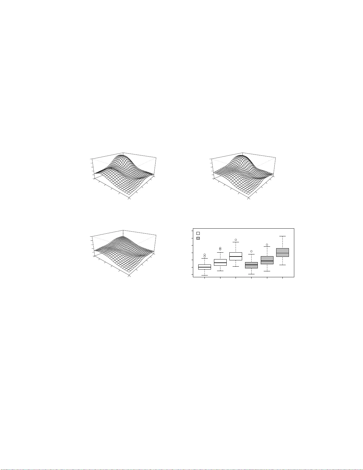
Submitted to the Annals of Appl ie d St atistics PENALIZED LIKELIHO OD REGR ESSION IN REPR ODUCING KERNEL HILBER T SP A CES WITH RANDOMIZED CO V ARIA TE D A T A By Xiwen Ma ∗ , Bin D ai ∗ , Ronald Klein † , Barbara E.K. Klein † , Kristine E. Lee ‡ and Gra ce W ah ba ∗ University o f Wisc onsin Classica l p enalized lik elihoo d regression prob lems d eal with the case that the indep endent v ariables data are know n exactly . In p rac- tice, how ev er, it is common t o observe data with incomplete co v ariate information. W e are concerned with a fund amentally imp ortant case where some of the observ ations do not rep resent the exact cov ariate information, but only a probability distribution. In this case, th e max- im um p enalized likelihoo d method can b e still applied to estimating the regression funct ion. W e ﬁrst show that the maxim um pen alized lik elihoo d estimate exists un der a mild condition. In the compu t ation, w e prop ose a dimension reduction technique to minimize th e p enal- ized likeli ho od and derive a GACV (Generalized Approximate Cross V alidation) to choose the smoothin g parameter. Ou r meth od s are ex- tended to handle more complicated incomplete data prob lems, such as, cov ariate measuremen t error and partially missing cov ariates. Con ten ts. 1 In tro duction . . . . . . . . . . . . . . . . . . . . . . . 2 1.1 P enalized likelihoo d regression in repro d ucing kernel Hilb ert spaces . . . . . . . . . . . . . . . . . . . . . . . . . . . . . . . 2 1.2 Randomized co v ariate d ata and related p roblems . . . . . . . 3 1.3 Outline of p ap er . . . . . . . . . . . . . . . . . . . . . . . . . 5 2 Randomized co v ariate p enalized lik elihoo d estimation (theory) . . 5 3 Randomized co v ariate p enalized likel iho o d estimation (computation) 7 3.1 Quadrature p en alized lik elihoo d estimates . . . . . . . . . . . 8 3.2 Construction of quadrature rules . . . . . . . . . . . . . . . . 9 3.2.1 Univ ariate quadratur e rules . . . . . . . . . . . . . . . 9 3.2.2 Multiv ariate quadr ature rules . . . . . . . . . . . . . . 10 ∗ Researc h supp orted in part by NIH Grant EY09946, NSF Grant DMS-0604572, NSF Gran t DMS-0906818 and ONR Grant N 0014-09-1-0655 . † Supp orted in part by NIH Grant EY 06594, and by the Researc h to Preven t Blindness Senior S cien tiﬁc Inv estigator Aw ards, New Y ork, NY . ‡ Supp orted in part by NI H Grant EY06594. Keywor ds and phr ases: Penalized likelihoo d regression, reprodu cing kernel Hilbert spaces, ra ndomized co va riate data, generalized approximate cross v alidation, errors in v ariables, cov ariate measuremen t error, partially missing cov ariates. 1 2 MA, DAI, KLEIN , KLEIN, LEE AND W AHBA 3.3 Choice of the smo othing parameter . . . . . . . . . . . . . . . 10 3.3.1 The comparativ e KL distance and lea vin g-out-one- sub ject CV . . . . . . . . . . . . . . . . . . . . . . . . 10 3.3.2 P arametric formulatio n of I Z, Π λ . . . . . . . . . . . . . 13 3.3.3 Generalized a v erage of submatrices, r andomized esti- mator . . . . . . . . . . . . . . . . . . . . . . . . . . . 13 3.3.4 The GA CV and rand omized GA CV . . . . . . . . . . 14 4 Co v ariate measurement error (mo del) . . . . . . . . . . . . . . . . 16 5 Co v ariate measurement error (computation) . . . . . . . . . . . . . 17 6 Missing co v ariate d ata (mo del) . . . . . . . . . . . . . . . . . . . . 18 6.1 Notatio ns and m o del . . . . . . . . . . . . . . . . . . . . . . . 1 8 6.2 Existence of th e estimator . . . . . . . . . . . . . . . . . . . . 20 7 Missing co v ariate d ata (computation) . . . . . . . . . . . . . . . . 20 8 Numerical Studies . . . . . . . . . . . . . . . . . . . . . . . . . . . 21 8.1 Examples of measur emen t error . . . . . . . . . . . . . . . . . 22 8.2 Examples of miss ing co v ariate data . . . . . . . . . . . . . . . 26 8.3 Case study . . . . . . . . . . . . . . . . . . . . . . . . . . . . 30 9 Conclud ing remarks . . . . . . . . . . . . . . . . . . . . . . . . . . 34 A T ec hnical pro ofs . . . . . . . . . . . . . . . . . . . . . . . . . . . . 35 B Deriv ation of GACV . . . . . . . . . . . . . . . . . . . . . . . . . . 39 C Extension to SS-ANOV A mo del . . . . . . . . . . . . . . . . . . . . 43 Ac kn o wledgmen ts . . . . . . . . . . . . . . . . . . . . . . . . . . . . . 44 References . . . . . . . . . . . . . . . . . . . . . . . . . . . . . . . . . . 44 Author’s addresses . . . . . . . . . . . . . . . . . . . . . . . . . . . . . 46 1. In tro duction. 1.1. Penalize d likeliho o d r e gr ession in r epr o ducing kernel Hilb ert sp ac es. W e are concerned with non or semi p arametric regression for d ata from a n on-Gaussian exp onential family . Supp ose that w e h a v e n in dep end en t observ ations ( y i , x i ) , i = 1 , ..., n , where eac h y i denotes the r esp onse and eac h x i denotes the co v ariate in f ormation. The goal is to ﬁt a probabilit y mec h anism, assu m ing that the conditional distribution of y i giv en x i has a densit y in th e exp onential family with the form p ( y i | x i , f ) = exp { ( y i · f ( x i ) − b ( f ( x i ))) /a ( φ ) + c ( y i , φ ) } (1.1) where b ( · ) and c ( · ) are giv en functions with b ( · ) s tr ictly con v ex, φ is the scale p arameter and f is the regression fu nction to b e estimated. W e assume PENALIZED LI KELIHOOD WITH RAND OMIZED COV AR IA TE 3 throughout this p ap er that φ is kn o w n, as, for example, Binomial data and P oisson data. In this case, ( 1.1 ) can b e simpliﬁed by p ( y i | x i , f ) = exp { y i · f ( x i ) − b ( f ( x i )) + c ( y i ) } . (1.2) Note th at the metho ds of this pap er can also b e extend ed to the situation when φ is unk n o wn, but ma y b e more computationally complicated. The regression fu nction f will b e estimated non or s emi parametrically in some repro d ucing k ernel Hilb ert space (RKHS) H by minimizing the p enalized likeli ho o d I λ ( f ) = − 1 n n X i =1 log p ( y i | x i , f ) + λ 2 J ( f ) (1.3) where th e p enalt y J ( · ) is a norm or semi-norm in H with ﬁnite d imensional n ull sp ace H 0 = { f ∈ H | J ( f ) = 0 } and λ is the smo othing p arameter whic h balances the tradeoﬀ b etw een mo del ﬁtting and smo othn ess. In this case, if the null space H 0 satisﬁes some condition, sa ying that I λ ( f ) has a unique min imizer in H 0 , then the minimizer of I λ ( f ) in H exists in a kno wn n -dimensional sub space sp anned b y H 0 and functions of the repro ducing k er- nel. See, for example, Kimeldorf and W ah ba (197 1)[ 25 ], O ’Sulliv an, Y andell and Ra ynor (1983)[ 32 ], W ahba (1990)[ 35 ] and Xiang and W ahba (1996)[ 3 6 ]. This mo del b uilding tec hn ique, kno wn as p enalized likeli ho o d r egression with RKHS p enalt y , allo ws for more ﬂexibility than parametric r egression mo dels. W e will not review the general literature, other than to note t wo b o oks and references therein. W ah ba (1990)[ 35 ] oﬀers a general in tro duc- tion of sp line mo dels. Gu (2002)[ 17 ] comprehensiv ely reviews the smo othing spline analysis of v ariance (SS-ANOV A), an imp ortant imp lemen tatio n of p enalized likeli ho o d regression in multiv ariate function estimation. 1.2. R andomize d c ovariate data and r e late d pr oblems. In this pap er, the issue w e are concerned ab out is the situation where comp onen ts of x i are not observ able b ut only kno wn to h a v e come from a particular probability dis- tribution. This concept of rand omized co v ariate, without the requ ir emen t of an y actual measure of x i , is more ﬂexible than the common sens e of co v ariate measuremen t err or. In this case, a n atural likel iho o d-based appr oac h is to treat x i ’s as laten t v ariables and minimize a randomized ve rsion of p enalized lik elihoo d that integrate s x i ’s out of the like liho o d. Th is ap p roac h , h o wev er, t ypically leads to a non-conv ex and in ﬁnite dimensional optimization prob- lem in RKHS. Therefore we s hall ﬁrst pro v e that the randomized p enalized lik elihoo d is minimizable. T his is the sub ject of Section 2. Afterwards, tw o 4 MA, DAI, KLEIN , KLEIN, LEE AND W AHBA computational issues will b e addressed in Section 3: (1) how to numerically compute an estimator and (2) ho w to select the smo othing parameter. Randomized co v ariate data is a b asic v er s ion of in complete data. Our metho ds can b e extended to other incomplete d ata problems. F or example, in the surv ey or medical researc h, it is common to obtain data where the co v ariate s are m easured with error. More sp eciﬁcally , x i is not directly ob- serv ed b ut instead x er r i = x i + u i is obser ved, where u i , i = 1 , ..., n are iid random p ertur bations. F an and T ru ong (1993)[ 12 ] regarded this measure- men t error problem in the con text of non p arametric regression, using the metho ds based on kernel decon v olution. Their tec hnique w as later studied and extended b y , for example, Ioannides and Alevizo (1997) [ 21 ], S c hennac h (2004 )[ 31 ], Carr oll, Rup p ert and Stefanski (2006)[ 6 ] and Delaigle, F an and Carroll (2009)[ 11 ]. More recentl y , p enalized lik eliho o d regression ha v e b een considered in the measuremen t error literature. Carroll, Maca and Rupp ert (1999 )[ 5 ] suggested to use the S IMEX metho d (Co ok and Stefanski, 1994[ 9 ]) to b uild n onparametric regression mo dels including b oth k ernel regression and p enalized lik eliho o d regression. Berry , C arroll and Rupp ert (2001)[ 2 ] de- scrib ed Bay esian approac h es for s mo othing splines and r egression P-splines. Cardot, Cram b es, Kneip and Sarda (2007)[ 4 ] u sed the total least square metho d (V an Huﬀel and V andew alle, 1991 [ 33 ]) to compute a s mo othing spline estimat or from noisy co v ariates. Th ese pap ers mainly discussed the situation of Gaussian resp onses bu t very little literature concerns other re- sp onses. As a sequel to these w orks, in this pap er, w e tr eat measuremen t error as a sp ecial case of r andomized co v ariates, b ecause eac h x i can b e view ed as a random v ariable (ve ctor) distribu ted as x er r i − u i . Th er efore the metho dology of r andomized p enalized lik eliho o d estimate can b e emplo yed. W e will as w ell b e able to m ake an other mo dest extension to treat the imp ortant situation where some comp onents of some x i ’s are completely missing. I n this case, w e ma y write x i = ( x obs i , x mis i ), wh ere x obs i and x mis i denote th e observ ed and the missing comp onen ts. It is w ell-kno wn (Lit- tle and Rubin, 2002[ 29 ]) that a complete case analysis th at deletes the cases with miss ing information often leads to bias or ineﬃcien t estimate s. V arious metho d s for missing co v ariate data ha v e b een d ev eloped in the con text of parametric regression mo dels, but to date few metho ds h av e b een pr op osed f or nonp arametric p enalized lik eliho o d regression in RK HS. F or p arametric regression, one p opu lar approac h is the method of weig h ts initially pr op osed by Ibrahim (1990)[ 18 ]. His su ggestio n is to assum e th e x i ’s to b e in dep end en t ob s erv ations from a marginal distribu tion dep end- ing on some p arameters and to maximize the joint distribution of ( y i , x i ) b y the exp ectation-maximizati on (EM) algorithm. Discussions and exten- PENALIZED LI KELIHOOD WITH RAND OMIZED COV AR IA TE 5 sions of this metho d app ear in Ibr ahim, Lipsitz and Ch en (1999)[ 19 ], Hor- ton and Laird (199 9)[ 22 ], Huang, Chen and Ib rahim (2005 )[ 24 ], Ibr ahim, Chen, L ipsitz and Herring (2005) [ 20 ], Horton and Kleinman (2007)[ 23 ], C hen and Ib rahim (2006)[ 7 ], C hen, Z eng and Ibrahim (2007)[ 8 ] and elsewhere. Ibrahim’s metho d can also b e emp loy ed to b uild nonparametric regression mo dels. Actually , in the framew ork of Ibr ahim’s metho d, the missing com- p onents x mis i can b e view ed as a random vect or dep end ing on the observed comp onent s x obs i and the cov ariate marginal distribu tion. T h erefore in this pap er, missin g co v ariate data is treated as a sp ecial case of randomized co v ariate data, and thus our metho ds can b e extended. 1.3. Outline of p ap er. The rest of the p ap er is organized as follo ws. In Section 2, w e pr ov e the existence of the rand omized co v ariate p enalized lik e- liho o d estimation in the general smo othin g spline set-up. Comp utational tec hn iques are presen ted in Section 3. Sections 4 and 5 extend our metho ds to the problem of cov ariate measuremen t error. Sections 6 and 7 describ e p e- nalized likeli ho o d regression with missing co v ariate data. Section 8 pro vides some numerical results. W e conclude our pap er in S ection 9. 2. Randomized co v ariate p enalized lik eliho o d es timation (the- ory). Consider the general smo othing splin e set-up, where x is allo w ed to b e from some arbitrary index set T on which an RHKS can b e d eﬁ ned. Randomized co v ariate data is d eﬁned in the w a y that we “observ e” for eac h sub ject i a pr ob ability sp ac e ( X i , F i , P i ), rather than a realiza tion of x i , where X i ⊆ T denotes the domain of x i , F i is a σ − algebra and P i is a pr obabilit y measure ov er ( X i , F i ). In this case, eac h x i can b e treated as a laten t rand om v ariable. Thus, giv en a regression fun ction f , th e distribu tion of [ y i | f ] h as a density (2.1) p ( y i | f ) = Z X i p ( y i | x i , f ) dP i . Note that, th r oughout this pap er, we use the lab els [ A | B ] and p ( A | B ) to denote the conditional distr ibution of A giv en B and the d ensit y fun ction for this d istribution. According to ( 2.1 ), the p enalized like liho o d estimate of f is the minimizer of (2.2) I R λ ( f ) = − 1 n n X i =1 log Z X i p ( y i | x i , f ) dP i + λ 2 J ( f ) where R denotes the “rand omness” of the co v ariates and f is restricted on the Borel measur able sub set (2.3) H B = { f ∈ H : f is Borel measurable on ( X i , F i ) , i = 1 , ..., n } 6 MA, DAI, KLEIN , KLEIN, LEE AND W AHBA in wh ich the Leb esgue integ rals in ( 2.2 ) can b e deﬁned. It can b e shown that H B is a sub space of H . PR OPOSITIO N 2.1. H B is a subsp ac e of H . Pro of See Ap p end ix A.  This metho dology can b e r eferred to as randomized co v ariate p e - nalized likelihoo d est imation or R C-PLE . Note th at RC-PLE includes the classica l p enalized like liho o d regression where x i ’s are observed exactly . Actually , I R λ ( f ) equals I λ ( f ) if ev ery ( X i , F i , P i ) stands for a single p oint probabilit y . Ho wev er, computation of RC-PLE is extremely diﬃcult. Firstly , since eac h p ( y i | x i , f ) is log-conca ve as a function of f , I R λ ( f ) is in general not con v ex d u e to th e in tegrals. Secondly , if at least one ( X i , F i , P i ) has inﬁnite supp ort, then there is n o ﬁn ite dimen sional su bspace in whic h f λ is known a prio ri to lie, as can b e concluded fr om the argumen ts in Kimeldorf and W ah ba (1971)[ 25 ]. T herefore, w e shall ﬁrst p ro v e that I R λ ( f ) is minimizable and hen ce th e phrase “p enalized lik elihoo d estimate” is meaningful. Com- putational tec hniques will b e d escrib ed in S ection 3. Recall that for the classical p enalized likeli ho o d regression, the un ique so- lution in th e n ull space is suﬃcient to en s ure the existence of the p enalized lik elihoo d estimate. In the case of rand omized co v ariate data, we extend this condition as follo ws: ASSUMPTION A.1 (Null space condition). There exist exactly observ ed sub jects ( y k 1 , x k 1 ) , ( y k 2 , x k 2 ) , ..., ( y k s , x k s ) su c h that P s i =1 log p ( y k i | x k i , f ) has a uniqu e maximizer in H 0 . No w we state our main theorem. THEOREM 2.2. Under A.1, ∃ f λ ∈ H B such that I R λ ( f λ ) = inf f ∈H B I R λ ( f ) . Theorem 2.2 guaran tees the existence of the RC-PLE estimate, wh ic h justiﬁes the title of the p ap er. In particular, if the null sp ace of the p enalty functional J ( · ) con tains only constan ts, then A.1 can b e ignored. In this case, the p enalized lik eliho o d estimate alw a ys exists. Our pro of of the th eorem is based on lo wer-semico n tin uit y in the w eak top ology . W e ﬁ rst recall some d eﬁnitions. PENALIZED LI KELIHOOD WITH RAND OMIZED COV AR IA TE 7 DEFINITION 1. A sequence { f k } k ∈ N in a Hilb ert sp ace H is said to con- v erge w eakly to f if h f k , g i → h f , g i for all g ∈ H . Here h· , ·i denotes the inner pr o duct of H . DEFINITION 2. Let H b e a Hilb ert sp ace, a f u nctional γ : H → R is (w eakly) sequentially low er semicon tin uous at f ∈ H if γ ( f ) ≤ lim inf γ ( f k ) for any sequence { f k } k ∈ N that (we akly) con v erges to f . DEFINITION 3. Let H b e a Hilb ert space, a f unctional γ : H → R is p ositiv ely co erciv e if || f || H → + ∞ im p lies γ ( f ) = + ∞ . Here || · || H de- notes the norm of H . Theorem 2.2 can b e sh o w n by com b ining Pr op osition 2.3 and Lemmas 2.4-2.6 b elo w . Note that Prop osition 2.3 is obtained from Theorem 7.3.7 in Kurd ila and Z abarankin (2005)[ 27 ], P age 217. T he p r o ofs of lemmas are giv en in App endix A. PR OPOSITIO N 2.3. L et H b e a Hilb ert sp ac e. Supp ose that γ : M ⊆ H → R is p ositively c o er cive and we akly se que ntial ly lower semic ontinuous over the close d and c onvex set M , then ∃ f 0 ∈ M such that γ ( f 0 ) = inf f ∈M γ ( f ) . LEMMA 2.4. Under A.1, the p enalize d likeliho o d I R λ ( f ) is p ositively c o er- cive over H B . LEMMA 2.5. The functional log R X i p ( y i | x i , f ) dP i : H B → R is we akly se quential ly c ontinuous. LEMMA 2.6. The p enalty functional J ( · ) is we akly se quential ly lower semi-c ontinuous. Pro of of Theorem 2 .2. Consider the f u nctional I R λ : H B ⊆ H → R . Theorem 2.2 follo ws from Prop osition 2.2, Lemma 2.4-2.6 and Pr op osition 2.3  . 3. Randomized co v ariat e p enalized likelihoo d estimation (com- putation). In the preceding section, we theoretically extended p enalized lik elihoo d regression in RKHS to randomized co v ariate data, wh ere f w as restricted on the Borel measurable subspace H B . In p ractical app licatio ns, ho w ev er, w e often face the case that all functions in th e RKHS are Borel measurable. In this case, w e no longer n eed th e restriction ment ioned in 8 MA, DAI, KLEIN , KLEIN, LEE AND W AHBA ( 2.3 ). Th us, we wo uld like to pro ceed our discussion under the follo w ing condition ASSUMPTION A.2. Consider the Borel- σ ﬁeld of H (generated by the op en sets). Mapp ing: T → H x 7→ K x ( · ) = K ( · , x ) is Borel measurable for all ( X i , F i ), i = 1 , ...n . Here K ( · , · ) denotes the re- pro du cing kernel of H . Under A.2, by Theorem 90 of Berlinet and Thomas-Agnan (200 4)[ 1 ], Page 195, every fun ction in H is Borel m easurable. It can b e ve riﬁed that if the domain T ⊆ R d and ev ery F i is a Borel σ -ﬁeld, then A.2 is satisﬁed w ith • Ev ery con tinuous kernel; • Kernels built fr om tensor sums or pro d u cts of con tinuous k ernels; • An y radial b asis kernel K ( x, z ) = r ( || x − z || d ) such that r ( · ) is contin- uous at 0. Here || · || d denotes the us u al Euclidian norm. 3.1. Quadr atur e p enalize d lik eliho o d estimates. As previously d iscussed, there is in general no ﬁnite dimensional subspace in which th e R C-PLE estimate f λ is known a priori to lie, so direct computation is not attracti v e. In th is case we shall ﬁnd a ﬁ nite dimens ional appr oximati ng sub space and compute an estimator in this space. W e consider the follo w ing p enalized lik elihoo d : (3.1) I Z, Π λ ( f ) = − 1 n n X i =1 log m i X j =1 π ij p ( y i | z ij , f ) + λ 2 J ( f ) where Z = { z 11 , ..., z 1 m 1 , z 21 , ..., z nm n } with z ij ∈ T and Π = { π 11 , ..., π 1 m 1 , π 21 , ..., π nm n } w ith π ij > 0. In words, when we ev aluate the in tegrals on the righ t hand side of ( 2.2 ), eac h ( X i , F i , P i ) is replaced by a discrete probabilit y distribution deﬁned o v er { z i 1 , z i 2 , ..., z im i } with probabilit y mass function P ( x i = z ij ) = π ij , j = 1 , ..., m i . T h us z ij , 1 ≤ j ≤ m i and π ij , 1 ≤ j ≤ m i are referr ed to as no des and weigh ts of a quadrat ure rule for probabilit y measure P i . In ( 3.1 ), f is only ev aluated on a ﬁn ite n um b er of qu adrature no des. Und er A.1, it can b e seen from Theorem 2.2 and the argument s in Kimeldorf and W ah ba (1971)[ 25 ] that th e minimizer of I Z, Π λ ( f ) in H is in a ﬁ nite dimen- sional su bspace H Z spanned by H 0 and { K ( · , z ij ) : z ij ∈ Z } . Thus, I Z, Π λ ( f ) PENALIZED LI KELIHOOD WITH RAND OMIZED COV AR IA TE 9 can b e formulat ed as a p arametric p enalized lik elihoo d. Green (1990)[ 16 ] ga ve a general discussion on th e u se of the EM algorithm for parametric p enalized lik elihoo d estimation with incomplete data. His m etho d can b e extended to minimize I Z, Π λ ( f ). It can b e s h o wn that the E-step at iteration t + 1 has th e form of (3.2) Q ( f | f ( t ) ) = 1 n n X i =1 m i X j =1 w ( t ) ij · log p ( y i | z ij , f ) − λ 2 J ( f ) where f ( t ) is estimated at iteration t and the w eigh t (3.3) w ( t ) ij = π ij p ( y i | z ij , f ( t ) ) P k π ik p ( y i | z ik , f ( t ) ) indicates the cond itional probabilit y of [ z ij | y i , f ( t ) ]. The M-step u p dates f b y maximizing Q ( f | f ( t ) ) in H . Th is is straigh tforw ard b ecause − Q ( f | f ( t ) ) is seen to b e a w eigh ted complete data p enalized lik elihoo d . When the EM algo rithm con v erges, we will ob tain an estimato r ˆ f λ whic h appro ximates the R C-PLE estimate f λ . Note that ˆ f λ can b e interpreted as a minimizer of I R λ ( f ) when the integ rals are appr o ximated b y quadrature rules. Hence, this computational tec hnique is referr ed to as quadrat ure p enalized lik eliho o d estimation or QPLE . Th e motiv ation b ehind this approac h is that an eﬃcient quadrature rule often requires only a few n o des for a go o d approxima tion to the in tegral. This con v enien t p rop erty eases the computation b urden at eac h M-step. 3.2. Construction of quadr atur e rules. Construction of quadr ature ru les is a pr actica l issue. In order to deriv e more applicable results, we fu rther assume that eac h x i = ( x i 1 , ..., x id ) T is a rand om v ector, i.e., T ⊂ R d . 3.2.1. Univariate quadr atur e rules. Supp ose that x i is univ ariate (i.e., d = 1). I n this case, if x i is a catego rical rand om v ariable or exactly ob- serv ed, then ( X i , P i ) itself can b e u sed as a qu ad r ature rule. Otherwise, if x i is a con tin u ous random v ariable, we will construct a Gaussian quadra- ture rule . Devel opmen t of computational m etho ds and r ou tin es of Gaussian quadrature in tegrat ion formula e for probability measures is a mathematical researc h topic. W e w ill not survey the general literature here, other than to sa y th at the metho d s considered in this pap er can b e obtained f rom, Golub and W elsc h (1969)[ 15 ], F ernandes and Atc hley (2006)[ 13 ], Bosserhoﬀ (2008 )[ 3 ] and Rahman (2009)[ 30 ]. T hough a k -no de Gaussian quadrature rule t ypically r equires the ﬁr st 2 k moment s of th e m easur e P i to b e ﬁnite, 10 MA, DAI, KLEIN , KLEIN, LEE AND W AHBA this con v en tion can b e satisﬁed b y most p opular probabilit y distribu tions including normal, uniform, exp onen tial, gamma, b eta and others. Besides Gaussian quadrature rules, if x i has a densit y with resp ect to the Leb esgue measure, w e also consider a quadrature r u le w ith equally-spaced p oin ts. More sp eciﬁcally , supp ose th at x i ranges ov er [ a, b ], then w e tak e equally- spaced p oints in [ a, b ] as qu adrature n o des while the quadr ature w eigh ts are p rop ortional to the dens it y ev aluated at the c hosen n o des. Note that if a = −∞ (or b = + ∞ ), we set a = µ i − 3 σ i (or b = µ i + 3 σ i ) where µ i and σ i denote the ﬁrst and second moment s of P i . W e refer to this simple quadrature ru le as the grid quadrature rule . 3.2.2. Multivariate quadr atur e rules. Supp ose that x i = ( x i 1 , ..., x id ) T is a m u ltiv ariate random v ector (i.e., d > 1). In this case, a quadrature r ule can b e generated recursiv ely with one-dimensional conditional quad r ature rules. T h e algo rithm is su mmarized as follo ws: 1. Set s = 1. Compute the marginal distribution of x i 1 and generate a quadrature ru le for x i 1 b y using th e metho d for univ ariate r an d om v ariables. 2. Let { z ( s ) 1 , ..., z ( s ) m s } and { π ( s ) 1 , ..., π ( s ) m s } b e the quad r ature r ule generated for the marginal d istr ibution of ( x i 1 , ..., x is ) T . F or eac h z ( s ) j , 1 ≤ j ≤ m s , compute the one-dimensional conditional distribu tion of [ x i ( s +1) | ( x i 1 , ..., x is ) T = z ( s ) j ] Then generate a quadrature rule for this distribution, d enoted by { z ∗ j 1 , ..., z ∗ j n j } and { π ∗ j 1 , ..., π ∗ j n j } . Th en { (( z ( s ) j ) T , z ∗ j r ) T , 1 ≤ r ≤ n j , 1 ≤ j ≤ m s } and { π ( s ) j · π ∗ j r , 1 ≤ r ≤ n j , 1 ≤ j ≤ m s } comp ose a quadrature rule for the marginal distribution of ( x i 1 , ..., x is , x i ( s +1) ) T . 3. Set s = s + 1. Rep eat step 2 until s = d . The ord er that x ij ’s ju mp in to the algorithm is not imp ortan t. O n e ma y r e- arrange the order to simplify the computation of the qu adrature rules. F rom our exp erience, a quadrature rule with 7 to 12 n o des for eac h comp onen t of x i usually yields a ve ry go o d approximat ion. In this case, the ab o v e EM algorithm u s ually con v erges very rapidly . 3.3. Choic e of the smo othing p ar ameter. 3.3.1. The c omp ar ative KL distanc e and le aving-out-one-subj e ct CV . So far the smo othing p arameter λ , is assumed to b e ﬁxed. Choice of λ is a k ey problem in the p enalized like liho o d regression. F or n on -Gaussian d ata, PENALIZED LI KELIHOOD WITH RAND OMIZED COV AR IA TE 11 Kullbac k-Leibler (KL) distance is commonly used as the risk fun ction f or the estimator f λ (3.4) KL( f ∗ , f λ ) = 1 n n X i =1 E y 0 i | f ∗  log p ( y 0 i | f ∗ ) p ( y 0 i | f λ )  where f ∗ denotes the true regression fun ction and the exp ectatio n is tak en o ver y 0 i ∼ p ( y | f ∗ ) indep endent of y i . In order to estimate KL( f ∗ , f λ ), Xiang and W ah ba (1996)[ 36 ] prop osed genera lized appro ximat e cross v ali- dation (GA C V) b eginning with a lea ving-out-one argumen t to c ho ose the smo othing p arameter, wh ic h wo rks w ell for Bernoulli data. L in , W ahba, Xi- ang, Gao, Klein and Klein (200 0)[ 28 ] d eriv ed a randomized version of GA CV (ranGA CV) which is more computatio nally friendly for large data sets. In this section w e obtain a con v enient form of lea vin g-out-one-sub ject CV f or randomized co v ariate d ata and extend GA CV and randomized GACV to randomized co v ariate data in subsequent sections. In the situation wh en eac h observe d co v ariate is actually a probabilit y space ( X i , F i , P i ), [ y 0 i | f ] h as a density of (3.5) p ( y 0 i | f ) = Z X i p ( y 0 i | x i , f ) dP i . F ollo win g ( 3.4 ) and lea ving out the qu an tities whic h do not d ep end on λ , the comparativ e K L (CKL) distance can b e written as (3.6) C K L( λ ) = − 1 n n X i =1 E y 0 i | f ∗  log Z X i exp  y 0 i f λ ( x i ) − b ( f λ ( x i ))  dP i  . T o simp lify the n otation, let’s denote (3.7) L ( y , f , P i ) = log Z X i exp { y f ( x i ) − b ( f ( x i )) } dP i the log-lik eliho o d fun ction for randomized co v ariate data. Using ﬁ r st order T a ylor exp ansion to expand L at the p oint y i , w e hav e that L ( y 0 i , f λ , P i ) ≈ L ( y i , f λ , P i ) + ( y 0 i − y i ) ∂ L ∂ y ( y i , f λ , P i ) . (3.8) Direct calculation yields ∂ L ∂ y ( y i , f λ , P i ) = R X i f λ ( x i ) exp { y i f λ ( x i ) − b ( f λ ( x i )) } dP i R X i exp { y i f λ ( x i ) − b ( f λ ( x i )) } dP i = E x i | y i ,f λ f λ ( x i ) . (3.9) 12 MA, DAI, KLEIN , KLEIN, LEE AND W AHBA Plugging ( 3.8 ) and ( 3.9 ) in to ( 3.6 ), w e hav e that CKL( λ ) ≈ OBS( λ ) + 1 n n X i =1 E y 0 i | f ∗ ( y i − y 0 i ) E x i | y i ,f λ f λ ( x i ) = OBS( λ ) + 1 n n X i =1 ( y i − µ ∗ i ) E x i | y i ,f λ f λ ( x i ) (3.10) where µ ∗ i = E y 0 i | f ∗ y 0 i is the tru e mean resp onse and OBS( λ ) = − 1 n n X i =1 log Z X i exp { y i f λ ( x i ) − b ( f λ ( x i )) } dP i (3.11) is the observed log-lik eliho o d. Denote f [ − i ] λ the lea ving-out-one estimator, i.e., th e min imizer of I R λ ( f ) with the i th sub ject omitted. Sin ce E x i | y i ,f λ f λ ( x i ) is the p osterior mean estimate of f ∗ ( x i ), follo wing Xiang and W ahba (1996)[ 36 ], w e may replace µ ∗ i E x i | y i ,f λ f λ ( x i ) by y i E x i | y i ,f [ − i ] λ f [ − i ] λ ( x i ) and deﬁne the lea ving- out-one-sub ject cr oss v alidation (CV) by (3.12) CV( λ ) = OBS( λ ) + 1 n n X i =1 y i ( E x i | y i ,f λ f λ ( x i ) − E x i | y i ,f [ − i ] λ f [ − i ] λ ( x i )) . It can b e seen that ( 3.10 ) and ( 3.12 ) generaliz e th e complete d ata C KL and CV formulas prop osed in Xiang and W ah ba (1996)[ 36 ]. I f ˆ f λ denotes the QPLE estimate, then we ma y f urther approximat e ( 3.12 ) by quadr ature rules. More sp eciﬁcally , O BS( λ ) can b e ev aluated b y (3.13) [ OBS( λ ) = − 1 n n X i =1 log m i X j =1 π ij exp n y i ˆ f λ ( z ij ) − b ( ˆ f λ ( z ij )) o where z ij ’s and π ij ’s repr esen t no des and weig h ts of the quadr ature rules giv en in the preceding section. Deﬁne th e wei gh t functions (3.14) w ij ( τ ) = π ij exp { y i τ j − b ( τ j ) } P k π ik exp { y i τ k − b ( τ k ) } , j = 1 , ..., m i where τ = ( τ 1 , ..., τ m i ) T is an arbitrary v ector of length m i . Let us use the notations ~ f λi = ( ˆ f λ ( z i 1 ) , ..., ˆ f λ ( z im i )) T (3.15) ~ f [ − i ] λi = ( ˆ f [ − i ] λ ( z i 1 ) , ..., ˆ f [ − i ] λ ( z im i )) T . (3.16) PENALIZED LI KELIHOOD WITH RAND OMIZED COV AR IA TE 13 Then ( 3.9 ) yields E x i | y i , ˆ f λ ˆ f λ ( x i ) ≈ m i X j =1 w ij ( ~ f λi ) ˆ f λ ( z ij ) = m i X j =1 w λ,ij ˆ f λ ( z ij ) (3.17) E x i | y i , ˆ f [ − i ] λ ˆ f [ − i ] λ ( x i ) ≈ m i X j =1 w ij ( ~ f [ − i ] λi ) ˆ f [ − i ] λ ( z ij ) = m i X j =1 w [ − i ] λ,ij ˆ f [ − i ] λ ( z ij ) (3.18) where w λ,ij = w ij ( ~ f λi ) and w [ − i ] λ,ij = w ij ( ~ f [ − i ] λi ) equal the weigh ts at the ﬁnal iteration of the EM algorithm, resp ectiv ely , when ˆ f λ and ˆ f [ − i ] λ w ere com- puted. Ther efore a more conv enient v ersion of CV can b e obtained as (3.19) CV( λ ) ≈ [ OBS( λ ) + 1 n n X i =1 y i m i X j =1 ( w λ,ij ˆ f λ ( z ij ) − w [ − i ] λ,ij ˆ f [ − i ] λ ( z ij )) . 3.3.2. Par ametric formulation of I Z, Π λ . Based on ( 3.19 ) and b y us in g sev eral ﬁrst ord er T a ylor expan s ions, a generalized app ro ximate cross v al- idation (GA CV) can b e deriv ed for rand omized co v ariate d ata. Before w e pro ceed, we w ould lik e to establish some n otatio ns. As w e previously discussed, I Z, Π λ ( f ) can b e f ormulate parametrically as (3.20) I Z, Π λ ( ~ y , ~ f ) = − 1 n n X i =1 log m i X j =1 π ij p ( y i | f ij ) + λ 2 ~ f T Σ λ ~ f where ~ f = ( f 11 , ..., f 1 m 1 , f 21 , ..., f nm n ) T denotes the v ector of f ev aluated at { z ij , 1 ≤ i ≤ n, 1 ≤ j ≤ m i } , ~ y = ( ~ y T 1 ..., ~ y T n ) T with ~ y i = ( y i , ..., y i ) T b e- ing m i replicates of y i and Σ λ is the p ositiv e semi-deﬁnite matrix satisfying λJ ( f ) = ~ f T Σ λ ~ f . Note that m inimizing I Z, Π λ ( f ) in H is equiv alent to mini- mizing I Z, Π λ ( ~ y , ~ f ) in R m 1 + ··· + m n . Hence ~ f λ = ( ˆ f λ ( z 11 ) , ..., ˆ f λ ( z 1 m 1 ) , ˆ f λ ( z 21 ) , ..., ˆ f λ ( z nm n )) T minimizes ( 3.20 ). Similarly , w e can denote ~ f [ − i ] λ = ( ˆ f [ − i ] λ ( z 11 ) , ..., ˆ f [ − i ] λ ( z 1 m 1 ) , ˆ f [ − i ] λ ( z 21 ) , ..., ˆ f [ − i ] λ ( z nm n )) T the minimizer of ( 3.20 ) with i th sub- ject omitted. 3.3.3. Gener alize d aver age of su bmatric es, r andomize d estimator. T o de- ﬁne the GA CV and r andomized GA CV we use th e concept of generalized a v era ge of submatrices and its randomized estima tor introd uced in Gao, W ah ba, Klein and Klein (2001)[ 14 ] for the multiv ariate outcomes case. Let A b e a square matrix with submatrices A ii , 1 ≤ i ≤ n on the diagonal. 14 MA, DAI, KLEIN , KLEIN, LEE AND W AHBA Denote A ii = ( a i st ) m i × m i , 1 ≤ s, t ≤ m i . Because A ii ’s ma y ha v e diﬀerent dimensions, we calculat e for eac h A ii (3.21) δ i = 1 nm i n X k =1 m k X j =1 a k j j = 1 nm i tr ( A ) and (3.22) γ i =  0 , if m i = 1 1 / ( nm i ( m i − 1)) P n k =1 P s 6 = t a k st , if m i > 1 . Then the generalized a v erage of A ii is deﬁn ed b y (3.23) ¯ A ii = ( δ i − γ i ) I m i × m i + γ i · e i e T i =      δ i γ i · · · γ i γ i δ i · · · γ i . . . . . . . . . . . . γ i γ i · · · δ i      where e i = (1 , 1 ..., 1) T is the u n it v ector of length m i . In this case, the inv erse of ¯ A ii can b e easily obtained by (3.24) ¯ A − 1 ii = 1 δ i − γ i I m i × m i − γ i ( δ i − γ i )( δ i + ( m i − 1) γ i ) e i e T i . No w we discuss ho w to obtain a rand omized estimator of ¯ A ii . Let ǫ = ( ǫ T 1 , ..., ǫ T n ) T , w here ǫ i = ( ǫ i 1 , ..., ǫ im i ) T with eac h ǫ ij generated indep endentl y from N (0 , σ 2 ). Denote ¯ ǫ = (¯ ǫ 1 , ..., ¯ ǫ 1 , ¯ ǫ 2 , ..., ¯ ǫ n ) T the corresp onding mean vec- tor w ith m i replicates of ¯ ǫ i for eac h 1 ≤ i ≤ n , where ¯ ǫ i = 1 / √ m i P m i j =1 ǫ ij . Then we observ e the follo wing f acts E ǫ T Aǫ = σ · tr ( A ) (3.25) E  ¯ ǫ T A ¯ ǫ − ǫ T Aǫ  = σ · n X k =1 X s 6 = t a k st . (3.26) Th us, a r andomized estimate of ¯ A ii can b e obtained by r eplacing δ i and γ i with their unbiased estimates 1 nm i σ ǫ T Aǫ and 1 nm i ( m i − 1) σ (¯ ǫ T A ¯ ǫ − ǫ T Aǫ ). 3.3.4. The GACV and r andom ize d GA CV. W e now present the result of GA CV as follo w. Details of the deriv ation can b e f ou n d in App endix B. Denote H the inﬂuence matrix of ( 3.20 ) with resp ect to ~ f ev aluated at ~ f λ . W rite (3.27) H =      H 11 ∗ ∗ ∗ ∗ H 22 · · · ∗ . . . . . . . . . . . . ∗ ∗ · · · H nn      P m i × P m i PENALIZED LI KELIHOOD WITH RAND OMIZED COV AR IA TE 15 where eac h H ii is a m i × m i submatrix matrix on the diagonal with resp ect to to ( f i 1 , ..., f im i ) T . Deﬁne W i = diag( b ′′ ( ˆ f λ ( z i 1 )) , ..., b ′′ ( ˆ f λ ( z im i ))) th e diag- onal matrix of estimated v ariances. Let W = diag( W 1 , ..., W n ) b e the “big” v ariance m atrix for all the observ atio ns. Denote G = I − H W with subm a- trices G ii = I m i × m i − H ii W i , 1 ≤ i ≤ n on the d iagonal. No w let ¯ H ii and ¯ G ii denote the generalized av erage of submatrices H ii and G ii . Then the generalized appr o xim ate cross v alidati on (GA CV) can b e written as (3.28) GA C V( λ ) = [ OBS( λ ) + 1 n n X i =1 y i ( d i 1 , ..., d im i ) ¯ G − 1 ii ¯ H ii    y i − ˆ µ λ ( z i 1 ) . . . y i − ˆ µ λ ( z im i )    where ˆ µ λ ( z ij ) = b ′ ( ˆ f λ ( z ij )) denote the estimated mean r esp onse and (3.29) d ij = w λ,ij " ( y i − ˆ µ λ ( z ij ))( ˆ f λ ( z ij ) − m i X k =1 w λ,ik ˆ f λ ( z ik )) + 1 # . In practice, ho w ev er, computation of the inﬂuence matrix H for large data sets is exp ensiv e and may b e unstable. Note that, in order to compute ¯ H ii and ¯ G ii , w e only n eed the sum of traces and th e s um of oﬀ-diagonal en tries of H ii ’s and G ii ’s. Therefore, the exact computation of H and G can b e av oided using randomized estimates of ¯ H ii and ¯ G ii . T o d o this, w e ﬁrst generate a random p ertur bation vecto r ǫ = ( ǫ T 1 , ..., ǫ T n ) T , where ǫ i = ( ǫ i 1 , ..., ǫ im i ) T and ǫ ij ’s are iid fr om N (0 , σ 2 ). T hen compute the mean v ector ¯ ǫ = (¯ ǫ 1 , ..., ¯ ǫ 1 , ¯ ǫ 2 , ..., ¯ ǫ n ) T where ¯ ǫ i = 1 / √ m i P m i j =1 ǫ ij . Denote ~ f ~ y + ǫ λ and ~ f ~ y + ¯ ǫ λ the minimizers of ( 3.20 ) with the p ertu rb ed data ~ y + ǫ and ~ y + ¯ ǫ . Similarly , denote ~ f ~ y λ (= ~ f λ ) the min imizer with the original d ata. T o ease the computational burd en, we can set ~ f ~ y λ as the initial v alue for the EM algorithm of ~ f ~ y + ǫ λ and ~ f ~ y + ¯ ǫ λ . Because H is the inﬂuence matrix, we ha v e that (3.30) ~ f ~ y + ǫ λ ≈ ~ f ~ y λ + H ǫ, ~ f ~ y + ¯ ǫ λ ≈ ~ f ~ y λ + H ¯ ǫ. This yields (3.31) ǫ T H ǫ ≈ ǫ T ( ~ f ~ y + ǫ λ − ~ f ~ y λ ) , ¯ ǫ T H ¯ ǫ ≈ ¯ ǫ T ( ~ f ~ y +¯ ǫ λ − ~ f ~ y λ ) . Th us, a rand omized estimate of ¯ H ii can b e obtained as w e previously de- scrib ed. Also it is straightfo rwa rd to sh o w that (3.32) ǫ T Gǫ ≈ ǫ T ǫ − ǫ T W ( ~ f ~ y + ǫ λ − ~ f ~ y λ ) , ¯ ǫ T G ¯ ǫ ≈ ¯ ǫ T ¯ ǫ − ¯ ǫ T W ( ~ f ~ y + ¯ ǫ λ − ~ f ~ y λ ) 16 MA, DAI, KLEIN , KLEIN, LEE AND W AHBA whic h implies a randomized estimate of ¯ G ii . In ord er to reduce the v ari- ance of randomized trace estimat es, one ma y d r a w R in dep end en t p ertur- bation vecto rs ǫ 1 , ..., ǫ R and compu te for eac h ǫ r the rand omized estimates ˆ ¯ H r ii , 1 ≤ i ≤ n and ˆ ¯ G r ii , 1 ≤ i ≤ n . Then th e ( R -replicated) ranGA CV fu nc- tion is (3.33) ranGA CV( λ ) = [ OBS( λ )+ 1 nR R X r =1 n X i =1 y i ( d i 1 , ..., d im i )( ˆ ¯ G r ii ) − 1 ˆ ¯ H r ii    y i − ˆ µ λ ( z i 1 ) . . . y i − ˆ µ λ ( z im i )    . 4. Co v ariate measuremen t error (mo del) . C o v ariate measurement error is a common o ccurren ce in man y exp erimen tal settings includ ing su r- v eys, clinical tr ials and medical stud ies. S upp ose that x i = ( x i 1 , ..., x id ) T tak es v alues in the real space R d . I n the p resence of measur emen t error, x i is not directly observ ed but instead x er r i = x i + u i is observed, where u i , 1 ≤ i ≤ n are iid rand om errors, indep end en t of ( y i , x i ). T o estimate the regression function, our idea is to treat measuremen t error as a sp ecial case of r andomized co v ariate s. More sp eciﬁcally , eac h x i is considered as a ran- dom v ector distrib uted as x er r i − u i . When the error distr ibution is kno wn, the distribution for x i can b e obtained immediately , and therefore R C-PLE can b e directly emplo y ed without an y extra eﬀort. Ho wev er, in practical applications, we often face the case that the error distribution is unknown. O ne common appr oac h in the measurement er r or literature is to assume a parametric mo del for the error densit y and to estimate the unkn o wn parameters from th e data. Let p ( u i | θ ) denote the sp eciﬁed error density indexed b y a real v ector θ ranging o v er Θ ⊆ R q and let F ( u i | θ ) denote the corresp ond ing c.d.f. function. Since our goal is to estimate the regression function, θ is treated as a nuisance parameter. Giv en ( f , θ ), y i has a marginal densit y of (4.1) p ( y i | f , θ ) = Z R d p ( y i | x er r i − u i , f ) p ( u i | θ ) du i . Th us RC-PLE can b e extended b y (4.2) I E λ ( f , θ ) = − 1 n n X i =1 log Z R d p ( y i | x er r i − u i , f ) p ( u i | θ ) du i + λ 2 J ( f ) . In this case, we still need Ass u mption A.1 to obtain the existence of th e p enalized lik eliho o d estimate. In addition w e state the f ollo wing extra as- sumption wh ic h can b e s atisﬁed with most p arametric mo dels for the error PENALIZED LI KELIHOOD WITH RAND OMIZED COV AR IA TE 17 distribution. ASSUMPTION B.1. The c.d.f. fun ction F ( u | θ ) is con tinuous in θ f or any u ∈ R d and the parameter space Θ is compact. No w w e can sho w the existe nce of p enalized lik eliho o d estimate by the follo win g T h eorem whic h is actually a corollary to Theorem 2.2. THEOREM 4.1. Under A.1, A .2 and B.1, ther e exi st f λ ∈ H and θ λ ∈ Θ such that I E λ ( f λ , θ λ ) = inf f ∈H ,θ ∈ Θ I E λ ( f , θ ) . Pro of See Ap p end ix A.  5. Co v ariate measuremen t error (computation). In order to com- pute an estimato r, w e extend Q PLE describ ed in Section 3.1 as follo ws. De- note ( f ( t ) , θ ( t ) ) th e p arameters estimated at iteration t . Let z ( t ) j , 1 ≤ j ≤ m and π ( t ) j , 1 ≤ j ≤ m denote the quadrature r u le based on the d en sit y fu n c- tion p ( u | θ ( t ) ). Note that the qu adrature rules can b e generated u sing the metho d introd uced in Section 3.1. It is n ot hard to s ee that the E-step at iteration t + 1 is to compute the exp ectatio n of th e p enalized likeli ho o d − 1 n P n i =1 log p ( y i | x er r i − u i , f ) p ( u i | θ ) + λ 2 J ( f ) with resp ect to the conditional distributions [ u i | y i , x er r i , f ( t ) , θ ( t ) ] , 1 ≤ i ≤ n . Usin g the qu adrature rule, eac h [ u i | y i , x er r i , f ( t ) , θ ( t ) ] can b e app ro ximated by a d iscrete d istr ibution with su pp ort { z ( t ) j , 1 ≤ j ≤ m } and mass function P ( u i = z ( t ) j ) = w ( t ) ij , where (5.1) w ( t ) ij = π ( t ) j p ( y i | x er r i − z ( t ) j , f ( t ) ) P k π ( t ) k p ( y i | x er r i − z ( t ) k , f ( t ) ) . Th us the E-step can b e written as Q ( f , θ | f ( t ) , θ ( t ) ) = 1 n n X i =1 m X j =1 w ( t ) ij · log p ( y i | x er r i − z ( t ) j , f ) − λ 2 J ( f ) + 1 n n X i =1 m X j =1 w ( t ) ij · log p ( z ( t ) j | θ ) . (5.2) Then the M-step maximizes Q ( f , θ | f ( t ) , θ ( t ) ), which can b e done by sepa- rately maximizing a complete data p enalized lik eliho o d of f (5.3) 1 n n X i =1 m X j =1 w ( t ) ij · log p ( y i | x er r i − z ( t ) j , f ) − λ 2 J ( f ) 18 MA, DAI, KLEIN , KLEIN, LEE AND W AHBA and a complete data log likeli ho o d of θ (5.4) 1 n n X i =1 m X j =1 w ( t ) ij · log p ( z ( t ) j | θ ) . Therefore the M-step b ecomes a s tand ard problem w hic h can b e solved by m uc h existing soft w are. When the EM algorithm conv erges, we will obtain the QPLE estimate ( ˆ f λ , ˆ θ λ ). Finally , we show ho w to select the sm o othing parameter λ in the case of co v ariate measuremen t error. Note th at our goa l is to construct a go o d estimator of f , and θ is treated as a n uisance parameter. In other w ords, we only care ab out the goo d n ess of ﬁt of the ˆ f λ . Therefore λ can b e selected in the same wa y as randomized cov ariate data. T o do this, we ﬁrst estimate the error distribution by p ( u i | ˆ θ λ ) and then determine eac h cov ariate distribu tion P i according to the relation x i = x er r i − u i . After that, the metho d in tro duced in Section 3.3 can emp loy ed directly for the c hoice of λ . Correcting for measurement error is a broad statistical research topic. In the in terest of space, we only discuss the situation when w e hav e a p ara- metric mo del for the error distribu tion. I t wo uld b e p ossible to extend ou r metho d to other situations of measurement error. F or examp le, when ad- ditional data is av ailable, such as a sample from the error distrib ution or rep eated observ ations for some x i , we may estimate the error distribution more accurately by using other approac hes. Also, sometimes, the parametric mo del p ( u i | θ ) ma y not b e a v ailable and in th is case, w e ma y wan t to esti- mate the error distribution n onparametrically . These are inte resting topics for futur e r esearc h . 6. Missing co v ariate data (mo del). No w we describ e p enalized lik e- liho o d regression with missing cov ariate d ata. W e assum e the missing mec h- anism to b e missing at random. 6.1. Notations a nd m o del. Let x i = ( x i 1 , ..., x id ) denote the vect or of co v ariate s ranging o ver a sub space of R d . By the idea of I b rahim’s metho d of w eigh ts (Ib rahim, 1990[ 18 ] and Ibr ahim, Lipsitz and Chen, 1999[ 19 ]), we ﬁrst assume a parametric m o del for the marginal d ensit y of x i , denoted as p ( x i | θ ) > 0, w here θ ∈ Θ ⊆ R q is a real ve ctor of indexing parameters. Here θ is tr eated as a n uisance parameter. W rite x i = ( x obs i , x mis i ) where x obs i is a v ector of observed comp onents and x mis i is a d i × 1 ve ctor of missing comp onents. F ollo wing Little and R u bin, (2002 )[ 29 ], the likelihoo d of ( f , θ ) can b e obtained b y in tegrating or su mming PENALIZED LI KELIHOOD WITH RAND OMIZED COV AR IA TE 19 out the missing comp onents in the joint densit y for ( y i , x i ) L ( f , θ ) = n X i =1 log Z R d i p ( y i | x i , f ) p ( x i | θ ) dx mis i (6.1) where R R d i p ( y i | x i , f ) p ( x i | θ ) dx mis i ≡ p ( y i | x i , f ) p ( x i | θ ) if x i is completely ob- serv ed. Then ( f , θ ) can b e estimat ed by minimizing the follo wing missin g data p en alized lik elihoo d : I M λ ( f , θ ) = − 1 n n X i =1 log Z R d i p ( y i | x i , f ) p ( x i | θ ) dx mis i + λ 2 J ( f ) . (6.2) W e note th at this metho d can b e view ed as an extension of R C-PLE. De- ﬁne P θ i,mis the probabilit y measur e o ver R d i , with resp ect to th e cond itional densit y of [ x mis i | x obs i ] (6.3) p ( x mis i | θ , x obs i ) = p ( x i | θ ) R R d i p ( x i | θ ) dx mis i , x mis i ∈ R d i . Note that ( 6.3 ) is w ell-deﬁned sin ce R R d i p ( x i | θ ) dx mis i < ∞ f rom the F u bini’s Theorem. Let (6.4) δ x obs i ( A ) =  1 if x obs i ∈ A 0 if x obs i / ∈ A denote the dirac measure deﬁn ed for x obs i . Consider the pro du ct measure P θ i = δ x obs i × P θ i,mis whic h satisﬁes that for any Borel sets A 1 ⊂ R d − d i , A 2 ⊂ R d i and their Cartesian pro d uct A 1 × A 2 , we ha ve (6.5) P θ i ( A 1 × A 2 ) = δ x obs i ( A 1 ) · P θ i,mis ( A 2 ) . Then it is not h ard to see that (6.6) I M λ ( f , θ ) = − 1 n n X i =1 log Z R d p ( y i | x i , f ) dP θ i + λ 2 J ( f ) − 1 n n X i =1 log Z R d i p ( x i | θ ) dx mis i is comp osed of a randomized co v ariate p enalized like liho o d of f and a log- lik elihoo d of θ . Hence missing co v ariate data can b e treated as a sp ecial case of randomized co v ariate data, allo wing co v ariate d istributions to b e ﬂexible. 20 MA, DAI, KLEIN , KLEIN, LEE AND W AHBA 6.2. Existenc e of the estimator. The follo wing assumptions can b e easily satisﬁed in the most exp erimen tal settings. ASSUMPTION M.1. D θ i = { x mis i ∈ R d i : p ( x i | θ ) > 0 } is compact for all 1 ≤ i ≤ n and θ ∈ Θ. ASSUMPTION M.2. The densit y fun ction p ( x | θ ) is contin uous in θ for an y x ∈ R d and the parameter space Θ is compact. The existence of the p enalized lik eliho o d estimate can b e guaran teed by the follo wing Theorem which is actually a corollary to Th eorem 2.2. THEOREM 6.1. Under A. 1, A.2, M.1 and M.2, ther e exist f λ ∈ H and θ λ ∈ Θ suc h that I M λ ( f λ , θ λ ) = inf f ∈H ,θ ∈ Θ I M λ ( f , θ ) . Pro of See Ap p end ix A.  7. Missing co v ariat e dat a (computation). In order to compu te an estimator, w e can extend QPLE in the same wa y as co v ariate measur emen t error. Denote ( f ( t ) , θ ( t ) ) the parameters estimated at iteration t . Let z ( t ) ij , 1 ≤ j ≤ m i and π ( t ) ij , 1 ≤ j ≤ m i denote th e quadrature ru le based on the probabilit y measure P θ ( t ) i deﬁned in ( 6.5 ). Then the E-step at iteration t + 1 can b e written as Q ( f , θ | f ( t ) , θ ( t ) ) = 1 n n X i =1 m i X j =1 w ( t ) ij · log p ( y i | z ( t ) ij , f ) − λ 2 J ( f ) + 1 n n X i =1 m i X j =1 w ( t ) ij · log p ( z ( t ) ij | θ ) (7.1) where (7.2) w ( t ) ij = π ( t ) ij p ( y i | z ( t ) ij , f ( t ) ) P k π ( t ) ik p ( y i | z ( t ) ik , f ( t ) ) . Then the M-step can b e done by sep arately maximizing (7.3) 1 n n X i =1 m i X j =1 w ( t ) ij · log p ( y i | z ( t ) ij , f ) − λ 2 J ( f ) PENALIZED LI KELIHOOD WITH RAND OMIZED COV AR IA TE 21 and (7.4) 1 n n X i =1 m i X j =1 w ( t ) ij · log p ( z ( t ) ij | θ ) whic h is computationally straigh tforw ard assuming the log-conca vit y of p ( x | θ ) as a function of θ . Again, when the EM algorithm con v er ges, the QP LE es- timate ( ˆ f λ , ˆ θ λ ) can b e obtained. In order to select the smo othing parameter, w e note that θ is a nuisance parameter and the choic e of λ only dep en ds on the go o dness of ﬁt of ˆ f λ . Therefore, we m a y select λ in the s ame wa y as r andomized co v ariate data. This is straightforw ard, since w e can tak e P ˆ θ λ i deﬁned in ( 6.5 ) as the co v ari- ate distribu tion. After that the metho d in Section 3.3 can emplo yed directly . F ollo win g Ibrahim, Lipsitz and Chen (1999)[ 19 ], our metho d can also b e extend ed to the non-ignorable missing data mec h anism. In this case, w e ma y sp ecify a parametric mo del for the m issing data mec hanism and incorp orate it in to the p enalized like liho o d. The extension is similar but more complicated. Thus this is another topic for fu tu re researc h. 8. Numerical Studies. In this section, we illustrate our metho d by sev eral sim u lated examp les with co v ariate measuremen t error and missing co v ariate s. F or eac h sim ulated data set, we will compare: (a) QPLE; (b) f ull data analysis b efore measurement error or missing co v ariates; and (c) n aiv e estimator that ignores measurement error or lea v es out the observ ations with missing co v ariates. Note that the c hoice of the smo othing parameter h as strong eﬀect on the p enalized likel iho o d estimator. Hence in order to show the p oten tial gain of our method , for eac h d ata set, λ is selecte d by b oth ranGA CV and the optimal v alue th at minimizes the Theoretical Kullback- Leibler distance (TKL), wh ic h do es n ot d ep end on the nuisance parameter θ . (8.1) TKL = 1 n n X i =1 E y 0 i | x i ,f ∗ ( log p ( y 0 i | x i , f ∗ ) p ( y 0 i | x i , ˆ f ) ) where f ∗ is the true r egression function, ˆ f den otes its estimator and x i denotes th e true co v ariate vec tor b efore measur ement error or ’missing’. Note that tunin g by minimizing TKL is only a v ailable in a simulation study when the ”truth ” is known. Our n umerical studies fo cus on P oisson distribution and Bernoulli distri- bution whic h are also the cases in our r eal d ata s et. The goal is to illustr ate: • the gain of Q PLE; 22 MA, DAI, KLEIN , KLEIN, LEE AND W AHBA • the p erformance of r anGA C V; • the robustness of Q PLE to the choice of quadr ature rules. All th e simulat ions are condu cted usin g R-2.9.1 installed in Red Hat Enter- prise Linux 5. 8.1. Examples of me asur ement err or. Cubic spline regression is p erhaps the most p opular case of p enalized lik eliho o d regression. W e consider the follo win g examples from Binomial and Po isson d istr ibutions: (i) p ( y | x ) =  2 y  p ( x ) y (1 − p ( x )) 2 − y , y = 0 , 1 , 2, where p ( x ) = 0 . 63 x cos (2 π x ) + 0 . 36; (ii) p ( y | x ) = Λ( x ) y e − Λ( x ) /y ! , y = 0 , 1 , 2 ... , wh er e Λ( x ) = 16 e − 18( x − 0 . 4) 2 − 5 e − 7( x − 0 . 5) 2 + 5; (iii) Same distribution as (ii) except Λ( x ) = 10 6 ( x 11 (1 − x ) 6 ) + 10 4 ( x 3 (1 − x ) 10 ) + 2 whic h is a m o diﬁcation of Example 5.5 of Gu (2002) [ 17 ]. In eac h case, w e tak e X ∼ U [0 , 1] and generate a sample of n = 101 ( x, y ) pairs. F or eac h sample generated, measur ement errors are created with the follo win g scheme. W e ﬁrst randomly select ﬁve ( x, y ) pairs as complete ob- serv ations and then in th e rest of the 96 pairs, random errors are generated b y x i + u i , wh er e u i ’s are iid either N(0 , σ 2 ) or U[ − δ, δ ] for v arious v alues of the noise-to- signal r atio v ar( u ) / v ar ( X ). F or eac h generated data set, QPLE is conducted u sing either the Gaussian quadrature rule or the grid quadra- ture ru le, where the Gaussian quadrature rule is compu ted by the statmo d pac k age in R-2.9.1. Note that we generate the same n um b er of n o des for eac h n oisy x i . Simulatio n r esults are su mmarized by the follo wing ﬁgures. Figure 1 sh o ws the estimated cur v es from one simulated data set of case (i) with normal error and v ar( u ) / v ar( X ) = 0 . 25. QPLE is computed via Gaussian qu adrature wh ere 11 no des are created for eac h noisy x i . P anel (c) plots for eac h regression m etho d the b o x p lot of theoretical Ku llbac k -Leibler distances ( 8.1 ) calculated from 100 rep eated sim ulations. W e also rep ort in (d) the TKL distances calculated in the same simulatio n setting except that u is u niform (with the s ame noise-to-signal r atio). PENALIZED LI KELIHOOD WITH RAND OMIZED COV AR IA TE 23 0.0 0.2 0.4 0.6 0.8 1.0 0.0 0.4 0.8 (a) Normal error s, TKL T uning x p(x) T r ue QPLE Full Naive 0.0 0.2 0.4 0.6 0.8 1.0 0.0 0.4 0.8 (b) Normal error s, ranGA CV T uning x p(x) T r ue QPLE Full Naive Full QPLE Naive Full QPLE Naive 0.00 0.10 0.20 (c) TKL/ranGA CV , normal errors TKL T uned by TKL T uned by ranGACV Full QPLE Naive Full QPLE Naive 0.00 0.10 0.20 (d) TKL/ranGA CV , uniform err ors TKL T uned by TKL T uned by ranGACV Fig 1 . Estimate d curves and TKL distanc es for c ase (i). Panels (a) and (b) c omp ar e the tar get (T rue) curve, and thr e e estimate d curves obtaine d fr om the f ul l data analysis (F ul l), the QPLE estimate, and the Naive estimate. (a) T uning: T K L, (b) T uning: r anGACV. In (a) and (b) u ∼ N (0 , 0 . 1 45 2 ) , assume d known. Panels (c) and (d) pr ovide plots of TKL distanc es. (c) u ∼ N (0 , 0 . 14 5 2 ) , assume d known. (d) u ∼ U [ − 0 . 25 , 0 . 25] , assume d known. 24 MA, DAI, KLEIN , KLEIN, LEE AND W AHBA Remark 1 Thr oughout Se ction 8, the choic e of the curves to display fr om the various 100 simulations is primarily subje ctive but de eme d to b e typic al of the b ulk of the visual images of the c omp arisons b etwe en the estimates. An ide a of the sc atter in the TKL distanc es over the 100 simulations may b e se en in the b ox plots. Figure 2 sho ws the estimated cu r v es from one sim ulation for case (ii) with uniform error and v ar( u ) / v ar ( X ) = 0 . 3. W e assu me th at δ is un kno wn when QPLE is conducted. A t eac h EM iteration, we use Gaussian quadrature and create 9 no des for eac h noisy x i . Panel (c) sh o ws the T KL distances from 100 simulat ions. Panel (d ) is obtained in the same simulat ion setting except that u is normal (with the same n oise-to- signal ratio), σ is u nknown. Our results indicate the signiﬁcan t gain of QPLE, when th e smo othing p a- rameter is selected by either TKL or ranGA CV. As w e p r eviously d iscussed, QPLE incorp orates the information ab out the error distr ib ution and hence is more informativ e. Generally sp eaking, wh en measurement errors are ig- nored, the estimated curve of naiv e metho d tends to b e ov ersmo othed and more biased near the mo des and b oundaries. S im ilar p henomenon has b een noted for other nonparametric regression metho d s, for example, Lo cal p oly- nomial estimate, as in Delaigle, F an and Carroll (2009)[ 11 ]. F or the choic e of smo othing p arameter, the p rop osed ranGACV inherits the prop ert y of tra- ditional ranGACV. As simulati ons suggest, it is capable of p ic kin g λ close to its optimal v alue even when θ is estimated. W e summarize the inﬂuence of quadrature rules on QPLE at Figure 3 , using case (iii) with normal error and v ar( u ) / v ar( X ) = 0 . 25. In the compu ta- tion, v ar( u ) is assu med to b e unknown and λ is selected b y TKL . W e consider four QPLE estimators (QPLE1, QPLE 2, QP LE3 and QP LE4) compu ted via, r esp ectiv ely , Gaussian quadrature, grid quadrature, Gaussian qu adra- ture when u is wrongly assum ed to b e uniform and grid quadrature when u is wrongly assumed to b e uniform. W e ﬁrst compare these quadrature rules b y setting the n um b er of no des (for eac h noisy x i ) to b e 11. The top tw o panels sh o w the estimated curv es from one sim ulation and panel (c) rep orts the TKL distances calculated from 100 sim ulations. Then we study the inﬂ u- ence of th e n um b er of th e n o des. On panel (d), we plot for eac h quadratur e the mean TKL distance (b ased on 100 sim ulations) ve rsus the num b er of no des. F rom the sim ulation results, we observ ed no signiﬁ can t d iﬀeren ce b e- t w een Gaussian quadr ature and grid qu adrature, though, as w e exp ected, Gaussian qu adrature is more eﬃcien t. Surp risingly , eve n with a wrong er- ror d istribution presp eciﬁed, th e p oten tial gain of QPLE is s till signiﬁcant. Hence we ma y sa y that QPLE is robust to the c hoice of the quadr atur e. W e PENALIZED LI KELIHOOD WITH RAND OMIZED COV AR IA TE 25 0.0 0.2 0.4 0.6 0.8 1.0 5 10 15 20 (a) Uniform err ors, TKL T uning x Λ ( x ) T r ue QPLE Full Naive 0.0 0.2 0.4 0.6 0.8 1.0 5 10 15 20 (b) Uniform err ors, ranGA CV T uning x Λ ( x ) T r ue QPLE Full Naive Full QPLE Naive Full QPLE Naive 0.0 0.2 0.4 0.6 0.8 (c) TKL/ranGA CV , uniform err ors TKL T uned by TKL T uned by ranGACV Full QPLE Naive Full QPLE Naive 0.0 0.2 0.4 0.6 (d) TKL/ranGA CV , normal errors TKL T uned by TKL T uned by ranGACV Fig 2 . Estimate d curves and TKL di stanc es for c ase (ii). Panels (a) and (b) c omp ar e the tar get (T rue) curve, and thr e e estimate d curves obtaine d fr om the f ul l data analysis (F ul l), the QPLE estimate, and the Naive estimate. (a) T uning: TKL, (b) T uning: r anGACV. In (a) and (b) u ∼ U [ − 0 . 27 3 , 0 . 273] , δ = 0 . 273 assume d unknown. Panels (c) and (d) pr ovide pl ots of TKL distanc es. (c) u ∼ U [ − 0 . 273 , 0 . 273 ] , δ = 0 . 273 assume d unknown. (d) u ∼ N (0 , 0 . 158 2 ) , σ = 0 . 158 assume d unknown. 26 MA, DAI, KLEIN , KLEIN, LEE AND W AHBA also note th at QPLE d o es not r equire a large n um b er of qu adrature no des to compute a go o d estimator. There is not m uc h gain to create more no des if w e already h a ve enough. Hence, in our numerical exp eriments, we generally compute 7-12 n o des for eac h n oisy or missin g comp onen t in th e co v ariate s. 0.0 0.2 0.4 0.6 0.8 1.0 0 5 10 15 20 25 (a) Normal error s, correctly assumed normal x Λ ( x ) T r ue Full Naive QPLE1 QPLE2 0.0 0.2 0.4 0.6 0.8 1.0 0 5 10 15 20 25 (b) Normal error s, incorrectly assumed unif orm x Λ ( x ) T r ue Full Naive QPLE3 QPLE4 Full QPLE1 QPLE2 QPLE3 QPLE4 Naive 0.0 0.2 0.4 0.6 0.8 (c) TKL distances by quadrature e xample TKL 0.0 0.2 0.4 0.6 (d) TKL distances by number of nodes number of nodes mean TKL 5 7 9 11 15 19 QPLE1 QPLE2 QPLE3 QPLE4 Full Naive Fig 3 . Estimate d curves and TKL distanc es for c ase (iii). u ∼ N (0 , 014 5 2 ) , assume d unknown. T uning: TKL. Panels (a) and (b) give the tar get curve, and estimate d curves fr om F ul l and Nai ve estimate. Panel (a) c omp ar es the Gaussian quadr atur e (QPLE1) and the grid quadr atur e (QPLE2) when the err ors ar e c orr e ctly assume d to b e zer o-me an normal (with unknown varianc e), and p anel (b) c omp ar es the Gaussian quadr atur e (QPLE3) and the grid quadr atur e (QPLE4) when the err ors ar e inc orr e ctly assume d to b e uniform (with unknown r ange); (a) and (b) use 11 no des. Panel (c) plots TKL distanc es, using 11 no des. Panel (d) plots me an TKL versus numb er of no des. The dotte d upp er and solid lower lines r epr esent the me an TK L for the naive metho d and the ful l data analysis. . 8.2. Examples of missing c ovariate data. In this section, w e consider F rank e’s “principal test function” T ( x ) = 3 4 e − ((9 x 1 − 2) 2 +(9 x 2 − 2) 2 ) / 4 + 3 4 e − ((9 x 1 +1) 2 / 49+(9 x 2 +1) 2 / 10) + 1 2 e − ((9 x 1 − 7) 2 +(9 x 2 − 3) 2 ) / 4 − 1 5 e − ((9 x 1 − 4) 2 +(9 x 2 − 7) 2 ) (8.2) PENALIZED LI KELIHOOD WITH RAND OMIZED COV AR IA TE 27 whic h wa s used as a test function of smo othing splin es in W ahba (1983 )[ 34 ]. T ( x ) is sho wn in Figure 4 . Consider the follo w in g examples x_1 0.0 0.2 0.4 0.6 0.8 1.0 x_2 0.0 0.2 0.4 0.6 0.8 1.0 T(x) 0.0 0.2 0.4 0.6 0.8 1.0 Fig 4 . F r anke’s princip al test function (i) Binomial distribu tion: p ( y | x ) =  5 y  p ( x ) y (1 − p ( x )) 5 − y , wher e (8.3) p ( x ) = 1 1 . 24 ( T ( x ) + 0 . 198); (ii) P oisson distribu tion: p ( y | x ) = Λ( x ) y e − Λ( x ) /y !, where (8.4) Λ( x ) = 15 T ( x ) + 3 . In eac h case, we take X = ( X 1 , X 2 ) ∼ U [0 , 1] × [0 , 1] and generate a s ample of n = 300 obs erv ations from the distr ibution of ( Y , X ). Afterw ards, a m iss ing data is created in a w a y that if y > 3 in case (i) or y > 10 in case (ii), we randomly tak e on e of the f ollo wing actions with equal pr obabilit y: (1) delete x 1 only; (2) delete x 2 only and (3) delete b oth x 1 and x 2 . On a v erage, we create 47 incomplete observ ations (out of 300) in case (i) and 61 incomplete observ ations in case (ii). W e will test our metho d b y thin plate spline regression. In order to im- plemen t Q PLE, we sp ecify for x a b iv ariate n ormal distribution N ( µ, Σ), where µ = ( µ 1 , µ 2 ) T and Σ = { σ ij } 2 × 2 (an arbitrary co v ariance matrix) are to b e estimated. At eac h EM iteration, w e construct for eac h incomplete x i 28 MA, DAI, KLEIN , KLEIN, LEE AND W AHBA x1 0.0 0.2 0.4 0.6 0.8 1.0 x2 0.0 0.2 0.4 0.6 0.8 1.0 p(x) 0.0 0.2 0.4 0.6 0.8 1.0 (a) Full x1 0.0 0.2 0.4 0.6 0.8 1.0 x2 0.0 0.2 0.4 0.6 0.8 1.0 p(x) 0.0 0.2 0.4 0.6 0.8 1.0 (b) QPLE x1 0.0 0.2 0.4 0.6 0.8 1.0 x2 0.0 0.2 0.4 0.6 0.8 1.0 p(x) 0.0 0.2 0.4 0.6 0.8 1.0 (c) Naive Full QPLE Naive Full QPLE Naive 0.02 0.06 0.10 0.14 (d) TKL/ranGA CV TKL T uned by TKL T uned by ranGACV Fig 5 . Estimate d functions of p ( x 1 , x 2 ) and TKL distanc es f or c ase (i). (a) F ul l data estimate. (b) QPLE estimate. (c) Naive estimate. The λ ’ s in (a), (b) and (c) ar e tune d by r anGACV. (d) Box plots of TKL distanc es when tune d by TKL and by r anGA CV. PENALIZED LI KELIHOOD WITH RAND OMIZED COV AR IA TE 29 x1 0.0 0.2 0.4 0.6 0.8 1.0 x2 0.0 0.2 0.4 0.6 0.8 1.0 Lambda(x) 0 5 10 15 20 (a) Full x1 0.0 0.2 0.4 0.6 0.8 1.0 x2 0.0 0.2 0.4 0.6 0.8 1.0 Lambda(x) 0 5 10 15 20 (b) QPLE x1 0.0 0.2 0.4 0.6 0.8 1.0 x2 0.0 0.2 0.4 0.6 0.8 1.0 Lambda(x) 0 5 10 15 20 (c) Naive Full QPLE Naive Full QPLE Naive 0.05 0.15 (d) TKL/ranGA CV TKL T uned by TKL T uned by ranGACV Fig 6 . Estimate d f unctions of Λ( x 1 , x 2 ) and TKL distanc es for c ase (ii). (a) F ul l data estimate. (b) QPLE estimate. (c) Naive estimate. The λ ’ s in (a), (b) and (c) ar e tune d by r anGACV. (d) Box plots of TKL distanc es when tune d by TKL and by r anGA CV. 30 MA, DAI, KLEIN , KLEIN, LEE AND W AHBA a Gauss ian q u adrature rule, wh ere 11 no des are created f or eac h m issing comp onent . Simulatio n results are su mmarized at Figure 5 and 6 . Figure 5 and 6 sho w the estimated fun ctions where the sm o othing pa- rameter is tun ed b y ranGACV. Th e b ottom right panel rep orts the TK L distances based on 100 simulations, w hen λ is selected b y TKL and ran- GA C V. T he p erf ormance of QPLE is also im p ressiv e in the case of missing co v ariate data. Note that most incomplete observ ations app eared n ear th e ‘p eak’ of the test function. In this case, if these incomplete observ ations are left out, w e will miss the information ab out th e p eak, as ind icated by the naiv e estimator. On th e other hand , by incorp orating most information in the data includ ing the observ ations with paritally missing co v ariates, QPLE pro vides encouraging results, ev en though w e actually sp eciﬁed a wrong co- v ariate d istr ibution. 8.3. Case study. In this section, we illustr ate our m etho d on an obser - v ational data set that has b een previously analyzed, by d eleting some co- v ariates, and then comparing our metho d with the original analysis and the naiv e metho d of dropp ing ﬁles with miss in g co v ariate s. The Bea ve r Dam Eye Stu dy is an ongoing p opu lation-based study of age-rela ted ocular disorders . Sub jects w ere a group of 4926 p eople aged 43-86 years at the start of the study wh o lived in Bea ver Dam, WI and w ere examined at baseline, b et ween 1988 an d 1990. A description of the p opulation and details of the study at baseline m a y b e found in Klein, Klein, Lin ton and Demets (1991 )[ 26 ]. Pigmenta ry abnormalities are one of the o cular disorders of int erest in that study . Pigmenta ry abnormalities are an early sign of age-rela ted macular degeneration and are d eﬁned by the presence of r etinal depigment ation and increased r etinal pigmen tation. Lin, W ah ba, Xiang, Gao, Klein and K lein (2000) [ 28 ] an d Gao, W ahba, Klein an d Klein(2001)[ 14 ] considered only th e n = 2545 wome m mem b ers of this cohort. 11 . 88% of them sho w ed evidence of pigmen tary abnormalities. They examined the asso ciation of pigmen tary abn ormalities with six other attributes at baseline, b y ﬁtting a Smo othing Spline ANOV A (SS-ANOV A) mo del. Th e six attributes are are listed in T able 1 . Let p ( x ) b e the probabilit y th at a sub ject with attribute v ecto r x at baseline will b e f ound to hav e a pigmen tary abnormalit y in at least one eye, at baseline. The mo del ﬁ tted w as of th e form f ( x ) = constan t + f 1 ( sy s ) + f 2 ( chol ) + f 12 ( sy s, chol ) (8.5) + d age · ag e + d bmi · bm i + d hor m · I 2 ( hor m ) + d drin · I 2 ( dr in ) . PENALIZED LI KELIHOOD WITH RAND OMIZED COV AR IA TE 31 Attributes unit range code systolic b loo d pressure mmH g 71-221 sys serum cholesterol mg /dL 102-503 chol age at baseline y ear s 43-86 ag e b od y mass index kg /m 2 15-64.8 bmi undergoing h ormone replacement therapy yes/no yes, no horm history of heavy drinking yes/ no yes,no drin T able 1 Covariates for Pigmentary Abnormalities Here x denotes the v ector of co v ariates listed in T able 1 and f ( x ) is the logit form of th e probabilit y: f ( x ) = log p ( x ) 1 − p ( x ) . The data analysis is summarized in Figure 7 , whic h is adapted from L in, W ah ba, Xiang, Gao, Klein and Klein (200 0)[ 28 ]. O n eac h panel, we plot the estimated probabilit y of pigmen tary abnormalities as a function of chol , f or v arious v alues of sy s, ag e and hor m . Note th at we only plot for b mi = 27.5 and drin = no, b ecause bmi has relativ ely small eﬀec t in the ﬁtted mo del while only 152 out of 2585 sub j ects hav e drin = 1. Hence Figure 7 is ade- quate to demons trate the estimated asso ciation patterns. Generally s p eaking, h igher chol w as asso ciated with a protectiv e eﬀect. Ho wev er, wh en chol go es from 250 to 350, a “bump” app ears on the es- timated curves. T h is phenomenon pro vides us a go o d opp ortunit y to test our metho d. In order to ‘hide’ the bu mp, w e create a data set with missing co v ariate s b y deleting some attribute v alues for those su b jects whose c h oles- terol is b et w een 250 and 350. Consequen tly , 517 incomplete sub jects are created with v alues of sys , bmi and horm r andomly remov ed. More exactly , 30 su b jects missed sys , bmi and horm , 109 sub jects missed b oth sys and bmi , 118 s ub jects missed b oth sys and horm and 260 sub ject s missed only one attribute v alue. W e s hall ﬁ rst claim that the metho dology in this pap er can b e extended to SS -ANO V A mo dels without any extra eﬀort, as illustrated in Ap p endix C. I n this case, QPLE can b e condu cted follo wing Ibrahim, Lipsitz and Chen (1999 )[ 19 ]. W e ﬁ rst mo del the join t co v ariate distribution via a sequen ce of one-dimensional cond itional distrib u tions. Note th at ( age , chol , drin ) are alw a ys observe d and h ence w e do not n eed to mo del them. Also, very f ew sub jects ha v e dr in = 1, hence dr in will b e ignored in the mo deling. Give n ( age , chol ), we adopt a biv ariate normal distribu tion ( sys , bmi ) ∼ N ( µ, Σ ), where µ = ( µ 1 , µ 2 ) with µ k = a k 0 + a k 1 sy s + a k 2 bmi, k = 1 , 2 and Σ = { σ ij } 2 × 2 is an arbitrary co v ariance matrix, and the a ’s and Σ are to b e estimated. No w conditionally on other attribu tes, hor m is mo deled via a 32 MA, DAI, KLEIN , KLEIN, LEE AND W AHBA 100 150 200 250 300 350 400 0.0 0.1 0.2 0.3 0.4 cholesterol(mg/dL) probability age =52, horm=no sys 157 sys 137 sys 123 sys 108 100 150 200 250 300 350 400 0.0 0.1 0.2 0.3 0.4 cholesterol(mg/dL) probability age =62, horm=no 100 150 200 250 300 350 400 0.0 0.1 0.2 0.3 0.4 cholesterol(mg/dL) probability age =71, horm=no 100 150 200 250 300 350 400 0.0 0.1 0.2 0.3 0.4 cholesterol(mg/dL) probability age =52, horm=yes 100 150 200 250 300 350 400 0.0 0.1 0.2 0.3 0.4 cholesterol(mg/dL) probability age =62, horm=yes 100 150 200 250 300 350 400 0.0 0.1 0.2 0.3 0.4 cholesterol(mg/dL) probability age =71, horm=yes Fig 7 . Pr ob ability curves estimate d f r om the ful l data analysis. This ﬁgur e is adapte d fr om Figur es 9 and 10 fr om Lin, Wahb a, Xiang, Gao, Klein and Klein (2000)[ 28 ] . Each p anel plots the estimate d pr ob ability of pigmentary abnormalities as a f unction of cholester ol, for four diﬀer ent values of sy s . The six p anels c orr esp ond to diﬀer ent values of ag e and horm , when drin =no and bmi =27.5 ar e ﬁxe d. PENALIZED LI KELIHOOD WITH RAND OMIZED COV AR IA TE 33 logistic regression mo del p ( hor m = 1) = exp { a 30 + a 31 ag e + a 32 chol + a 33 sy s + a 34 bmi } 1 + exp { a 30 + a 31 ag e + a 32 chol + a 33 sy s + a 34 bmi } . F ollo win g this constru ction of co v ariate d istributions and using the metho d describ ed in Sectio n 3.1, a quadr ature r ule can b e obtained recursiv ely at eac h EM iteratio n. In the computation, the num b ers of no des generated for sys , b mi and horm are 10, 10 and 2 resp ectiv ely . Results of QPLE are giv en at Figure 8 . Figure 9 shows the naive estimator computed ov er th e 2068 sub jects without missing co v ariates. 100 150 200 250 300 350 400 0.0 0.1 0.2 0.3 0.4 cholesterol(mg/dL) probability age =52, horm=no sys 157 sys 137 sys 123 sys 108 100 150 200 250 300 350 400 0.0 0.1 0.2 0.3 0.4 cholesterol(mg/dL) probability age =62, horm=no 100 150 200 250 300 350 400 0.0 0.1 0.2 0.3 0.4 cholesterol(mg/dL) probability age =71, horm=no 100 150 200 250 300 350 400 0.0 0.1 0.2 0.3 0.4 cholesterol(mg/dL) probability age =52, horm=yes 100 150 200 250 300 350 400 0.0 0.1 0.2 0.3 0.4 cholesterol(mg/dL) probability age =62, horm=yes 100 150 200 250 300 350 400 0.0 0.1 0.2 0.3 0.4 cholesterol(mg/dL) probability age =71, horm=yes Fig 8 . Pr ob ability curves obtaine d fr om QPLE. Each p anel plots the estimate d pr ob ability of pigmentary abnormalities as a function of cholester ol, for four diﬀer ent values of sy s . The six p anels c orr esp ond to diﬀer ent values of a g e and hor m , when drin = no and bmi =27.5 ar e ﬁxe d. Note th at only the incomplete sub jects con tain information ab out the bumps . Consequent ly , the n aiv e estimator omitted these bump s, leading to monotone d ecreasing pr obabilit y curves. In words, high choleste rol app ears to generally low er the risk of p igmen tary abnormalities esp eciall y in the 34 MA, DAI, KLEIN , KLEIN, LEE AND W AHBA older, hor m = no group, aside f rom th e “bump”, from the full data analysis sho wn at Figure 7 . Ho w ev er, the naive estimator app ears to mak e this risk decrease substantial ly more rapidly d ue to missing the “bump ” completely , while the QPLE did an excellen t job of reco v ering the original analysis– the QPLE estimated curves are very close to those of the full d ata analysis. This can b e un dersto o d from the fact that most of the incomplete sub jects missed only one or t w o (out of six) co v ariates. Hence most information is still r etained in the miss ing data. 100 150 200 250 300 350 400 0.0 0.1 0.2 0.3 0.4 cholesterol(mg/dL) probability age =52, horm=no sys 157 sys 137 sys 123 sys 108 100 150 200 250 300 350 400 0.0 0.1 0.2 0.3 0.4 cholesterol(mg/dL) probability age =62, horm=no 100 150 200 250 300 350 400 0.0 0.1 0.2 0.3 0.4 cholesterol(mg/dL) probability age =71, horm=no 100 150 200 250 300 350 400 0.0 0.1 0.2 0.3 0.4 cholesterol(mg/dL) probability age =52, horm=yes 100 150 200 250 300 350 400 0.0 0.1 0.2 0.3 0.4 cholesterol(mg/dL) probability age =62, horm=yes 100 150 200 250 300 350 400 0.0 0.1 0.2 0.3 0.4 cholesterol(mg/dL) probability age =71, horm=yes Fig 9 . Pr ob ability curves obtaine d fr om the naive metho d. Each p anel plots the estimate d pr ob abi lity of pigmentary abnormalities as a function of cholester ol, f or f our diﬀer ent val- ues of sy s . The six p anels c orr esp ond to diﬀer ent values of ag e and hor m , when drin =no and bmi =27.5 ar e ﬁxe d. 9. Concluding remarks. W e ha v e presen ted a direct extension of p e- nalized like liho o d regression to the s itu ation w hen the observed cov ariates are probabilit y spaces. The r egression function is estimated b y minimizing a p enalized lik eliho o d that incorp orates distrib utional inf ormation of the co v ariate s. Numerically , we compute a ﬁnite dim en sional estimator after appro ximating the integral s in the likeli ho o d fu nction b y quadrature ru les. PENALIZED LI KELIHOOD WITH RAND OMIZED COV AR IA TE 35 Using the same approximati on, GA C V and its randomized version hav e b een deriv ed to select the sm o othing p arameters. Our m etho d is computationally eﬃcien t, as it only require a small n um b er of quadrature no des to obtain a go o d estimate. A direct imp lementat ion of our metho d is to hand le in- complete cov ariate data suc h as co v ariate measuremen t error and partially missing co v ariates. In the examples w e h a v e inv estigated, the resulting es- timator substan tially outp erformed the n aiv e estimator and app eared to b e close to the full d ata analysis. Our metho ds can also b e extend to other regularization settings, for ex- ample, the LASSO and supp ort v ecto r machine with hinge loss fu nction and L 2 p enalt y . In these cases, it might b e more complicated to dev elop a lik eliho o d-based frequentist app roac h . W e would like to inv estigate these extensions in th e futur e researc h. APPENDIX A: TECHNICAL PROOFS Pro of of Prop osition 2.1. An y linear com b in ation of measurable func- tions is still measurable. Th erefore it suﬃces to prov e that H B is complete. Let f 1 , f 2 , ... b e a C auc h y sequence in H B and f ∗ b e its limit in H . Then f 1 , f 2 , ... con v erge p oin t wise to f ∗ . Note that the p oin t wise limit of measur- able fun ctions is still a measurable fun ction. Therefore f ∗ ∈ H B .  No w to s imply the n otation in the pro ofs of Lemm a 2.4-2.6, let’s d eﬁne (A.1) l i ( t ) = y i · t − b ( t ) + c ( y i ) the log-densit y as a fun ction of th e natural parameter. Then l i ( t ) is strictly conca ve and b ounded fr om ab ov e. T herefore there are three p ossible cases of the limit of l i ( t ): (1) lim t →−∞ l i ( t ) = l i and lim t → + ∞ l i ( t ) = −∞ ; (A.2) (2) lim t →−∞ l i ( t ) = −∞ and lim t → + ∞ l i ( t ) = l i ; (A.3) (3) lim t →−∞ l i ( t ) = −∞ and lim t → + ∞ l i ( t ) = −∞ (A.4) where l i = sup t l i ( t ) < ∞ . Pro of of Lemma 2.4. Without loss of generalit y , we supp ose that A.1 is satisﬁed with the ﬁrs t m cases (hence they are completely observ ed). In order to sh ow Lemma 2.4, we ﬁ rst pr o v e that und er A.1, L ( f ) = P m i =1 log p ( y i | x i , f ) is p ositiv ely co erciv e o ver H 0 . Su pp ose to the cont rary that th is is not tru e. 36 MA, DAI, KLEIN , KLEIN, LEE AND W AHBA Then there exists a constant U > 0 and a sequence { g k } k ∈ N ⊆ H 0 with || g k || H = 1 s uc h that (A.5) − m X i =1 l i ( k · g k ( x i )) ≤ U, k ∈ N . Since the unit sph ere { g ∈ H 0 : || g || H = 1 } is sequence compact, there exists a subsequence { g k j } j ∈ N con v erging to some g ∗ with || g ∗ || H = 1. W e claim that (A.6) g ∗ ( x i )    ≤ 0 , if i b elongs to Case 1 as ( A.2 ) ≥ 0 , if i b elongs to Case 2 as ( A.3 ) = 0 , if i b elongs to Case 3 as ( A.4 ) . Supp ose to the con trary that ( A.6 ) is n ot true. If i b elong to case (1), then g ∗ ( x i ) = a > 0. S ince { g k j } j ∈ N con v erges to g ∗ , there exists N > 0 suc h that (A.7) g k j ( x i ) ≥ a/ 2 , f or all j > N . F rom ( A.5 ), w e hav e (A.8) l i ( k j · g k j ( x i )) ≥ U − X s 6 = i l s < ∞ , j ∈ N . This is a con tradiction of ( A.2 ) since when j > N (A.9) k j · g k j ( x i ) ≥ k j · a/ 2 → + ∞ . Similar con trad iction can b e observ ed wh en i b elongs to case (2) or case (3). Therefore the claim in Equation ( A.6 ) follo ws. No w let g 0 b e the u nique m in imizer of − P m i =1 l i ( g ( x i )) in H 0 . C onsider g 0 + r g ∗ with r > 0. Combining ( A.2 )–( A.4 ) and ( A.6 ), w e can see that (A.10) − m X i =1 l i ( g 0 ( x i ) + r g ∗ ( x i )) ≤ − m X i =1 l i ( g 0 ( x i )) , ∀ r > 0 . But this is a con tradiction. Hence L ( f ) is p ositiv ely co erciv e o ver H 0 , wh ic h means that (A.11) || g || H → ∞ ⇒ − m X i =1 l i ( g ( x i )) → + ∞ , g ∈ H 0 . Consider the orthogonal decomp osition f = g + h where g ∈ H 0 T H B and h ∈ H 1 T H B . The L emma can b e pro v ed in steps. PENALIZED LI KELIHOOD WITH RAND OMIZED COV AR IA TE 37 (i) || h || H → + ∞ . In this case (A.12) I R λ ( f ) ≥ − 1 n n X i =1 l i + 1 2 λ || h || H → + ∞ . (ii) || h || H ≤ U for some U > 0 bu t || g || H → + ∞ . In this case | h ( x i ) | = |h h, K ( · , x i ) i| ≤ || h || H K 1 / 2 ( x i , x i ) ≤ U · K 1 / 2 ( x i , x i ) , i = 1 , 2 , ...m whic h implies th at f ( x i ) = g ( x i ) + h ( x i ) = g ( x i ) + O (1) , i = 1 , ..., m, || h || H ≤ U. Let || g || H → ∞ , w e ha v e I R λ ( f ) ≥ − 1 n n X i =1 log Z X i p ( y i | x i , f ) dP i ≥ − 1 n m X i =1 l i ( g ( x i ) + h ( x i )) − 1 n n X j = m +1 l j = − 1 n m X i =1 l i ( g ( x i ) + O (1)) − 1 n n X j = m +1 l j → + ∞ (A.13) where ( A.13 ) follo ws f rom the claim in Equation ( A.11 ). The Lemma is no w prov ed b y com bining (i) and (ii).  Pro of of Lemma 2.5. Let { f k } k ∈ N b e a sequ en ce in H B whic h con- v erges w eakly to f ∗ . Since p oin t w ise limit of measurable fu nctions is still a measurable fu nction, f ∗ ∈ H B . F rom the con tin u it y of l i ( t ), { e l i ( f k ( x i )) } k ∈ N p oint wise con v erges to e l i ( f ∗ ( x i )) o ver X i . Note that e l i ( f k ( x i )) ≤ e l i and ev- ery constant is integrable with r esp ect to ( X i , F i , P i ). By the Dominated Con v ergence Theorem, w e hav e that lim k →∞ Z X i e l i ( f k ( x i )) dP i = Z X i e l i ( f ∗ ( x i )) dP i . (A.14) The Lemma no w follo ws since log( · ) is con tin uous.  Pro of of Lemma 2.6. Let { f k } k ∈ N b e a sequ ence in H B whic h w eakly con v erges to f ∗ . Consider the orthogonal d ecomp osition of eac h f k b y f k = 38 MA, DAI, KLEIN , KLEIN, LEE AND W AHBA g k + h k with g k ∈ H 0 T H B and h k ∈ H 1 T H B . It is straigh tforw ard to see that { h k } k ∈ N w eakly con v erges to h ∗ , the smo oth part of f ∗ . Therefore w e can write (A.15) 0 ≤ || h k − h ∗ || 2 H = || h k || 2 H + || h ∗ || 2 H − 2 h h k , h ∗ i . Let k → ∞ , we observ e that 0 ≤ lim inf k || h k || 2 H − || h ∗ || 2 H (A.16) and the Lemma is p ro v ed b y d eﬁnition.  Pro of of Theorem 4.1. F or any ﬁxed θ ∈ Θ, by Theorem 2.2, I E λ ( f , θ ) is minimizable in H . Let (A.17) T ( θ ) , min f ∈H I E λ ( f , θ ) denote the min im um p enalized lik eliho o d give n θ . W e claim that T ( θ ) is con tin u ous. F or any sequence { θ k } k ∈ N ∈ Θ that con v erges to θ ∗ , let P θ k and P θ ∗ denote the probabilit y measures on R d with densit y functions p ( u | θ k ) and p ( u | θ ∗ ). S ince F ( u | θ k ) → F ( u | θ ∗ ) for any u ∈ R d , P θ k w eakly con verges to P θ ∗ . Note that, for any ﬁxed f ∈ H , G ( u ) , p ( y i | x er r i − u, f ) is a real-v alued, con tin u ous and b ounded fu nction on R d . T h us R G ( u ) dP θ k → R G ( u ) dP θ ∗ . Equiv alen tly , that is (A.18) Z R d p ( y i | x er r i − u i , f ) p ( u i | θ k ) du i → Z R d p ( y i | x er r i − u i , f ) p ( u i | θ ∗ ) du i whic h implies that I E λ ( f , θ ) is contin uous in θ for any ﬁx ed f . T his is suf- ﬁcien t to prov e the con tin u it y of T ( θ ). Th e theorem no w follo w s fr om the compactness of Θ .  . Pro of of Theorem 6.1. F or any ﬁ xed θ ∈ Θ, by ( 6.6 ) and T heorem 2.2, I M λ ( f , θ ) is minimizable in H . Thus, we can deﬁne (A.19) T ( θ ) , min f ∈H I M λ ( f , θ ) . W e claim that T ( θ ) is contin uous. By Assu mption M.1 and M.2, there exists U > 0 suc h that p ( x i | θ ) < U for all x mis i ∈ D θ i , θ ∈ Θ and 1 ≤ i ≤ n . No w for any sequence { θ k } k ∈ N ∈ Θ that PENALIZED LI KELIHOOD WITH RAND OMIZED COV AR IA TE 39 con v erges to θ ∗ , p ( y i | x i , f ) p ( x i | θ k ) p oint wise con v erges to p ( y i | x i , f ) p ( x i | θ ∗ ). Note th at p ( y i | x i , f ) p ( x i | θ k ) ≤ e l i · U and an y constan t is in tegrable on the compact domain D θ i . By Dominated Conv ergence Theorem, we conclude that (A.20) lim k →∞ Z D θ i p ( y i | x i , f ) p ( x i | θ k ) dx mis i = Z D θ i p ( y i | x i , f ) p ( x i | θ ∗ ) dx mis i whic h implies that I M λ ( f , θ ) is con tin u ou s in θ for an y ﬁ xed f . This is suf- ﬁcien t to prov e the con tin u it y of T ( θ ). Th e theorem no w follo w s fr om the compactness of Θ .  APPENDIX B: DERIV A TION OF GACV Our GACV is deriv ed b ased on the cross v alidation fu nction ( 3.19 ). Let us use the notations ( 3.15 ) and ( 3.16 ). It can b e seen fr om ( 3.1 8 ) that P m i j =1 w [ − i ] λ,ij ˆ f [ − i ] λ ( z ij ) can b e treated as a function of ~ f [ − i ] λi . Note that ~ f [ − i ] λi is exp ected to b e close to ~ f λi , Thus using the ﬁrst order T a ylor expansion to expand P m i j =1 w [ − i ] λ,ij ˆ f [ − i ] λ ( z ij ) at ~ f λi , we hav e that CV( λ ) ≈ [ OBS( λ ) + 1 n n X i =1 y i ( ~ f λi − ~ f [ − i ] λi ) T ∂ P m i j =1 w ij ( τ ) τ j ∂ τ    ~ f λi = [ OBS( λ ) + 1 n n X i =1 y i ( ~ f λi − ~ f [ − i ] λi ) T    d i 1 . . . d im i    (B.1) where w ij ( τ ) and d ij are deﬁned b y ( 3.14 ) and ( 3.29 ), resp ectiv ely . Thus, it remains to estimate ~ f λi − ~ f [ − i ] λi . T o do this, we ﬁrst extend the leav e-out-one lemma (Crav en an d W ahba,1 979[ 1 0 ]) to rand omized co v ariate data. LEMMA B.1 (le ave-out- one-subje ct lemma) L et l ( y i , t ) = y i · t − b ( t ) + c ( y ) b e the lo g-likeliho o d function and I Z, Π λ ( ~ y , f ) = − P n i =1 log P m i j =1 π ij exp { l ( y i , f ( z ij )) } + nλ 2 J ( f ) , wher e ~ y = ( ~ y T 1 ..., ~ y T n ) T with ~ y T i = ( y i , ..., y i ) T b eing m i r eplic ates of y i . Supp ose that τ = ( τ 1 , ..., τ m i ) T is a m i × 1 ve c tor and h λ ( i, τ , · ) is the minimizer in H of I Z, Π λ ( ~ Y , f ) , wher e ~ Y = ( ~ y T 1 , ..., ~ y T i − 1 , τ T , ~ y T i +1 , ..., ~ y T n ) T . Then (B.2) h λ ( i, ~ µ [ − i ] λi , · ) = ˆ f [ − i ] λ 40 MA, DAI, KLEIN , KLEIN, LEE AND W AHBA wher e ˆ f [ − i ] λ minimizes − P k 6 = i log P m k j =1 π k j exp { l ( y i , f ( z k j )) } + nλ 2 J ( f ) , and ~ µ [ − i ] λi = ( b ′ ( ˆ f [ − i ] λ ( z i 1 )) , ..., b ′ ( ˆ f [ − i ] λ ( z im i ))) T is the ve ctor of me ans c orr esp ond- ing to ˆ f [ − i ] λ . Pro of of L emma B.1. Firstly , we claim that (B.3) l ( b ′ ( ˆ f [ − i ] λ ( z ij )) , ˆ f [ − i ] λ ( z ij )) ≥ l ( b ′ ( ˆ f [ − i ] λ ( z ij )) , f ( z ij )) , 1 ≤ j ≤ m i , ∀ f ∈ H . This follo ws since ∂ l ( b ′ ( ˆ f [ − i ] λ ( z ij )) , t ) ∂ t = b ′ ( ˆ f [ − i ] λ ( z ij )) − b ′ ( t ) and u sing the fact that ∂ 2 l ( y ,t ) ∂ t 2 = − b ′′ ( t ) < 0. Therefore l ( b ′ ( ˆ f [ − i ] λ ( z ij )) , t ) ac h iev es its un ique maxim um for t = ˆ f [ − i ] λ ( z ij ). Deﬁne ~ y [ − i ] = ( ~ y T 1 , ..., ~ y T i − 1 , ( ~ µ [ − i ] λi ) T , ~ y T i +1 , ..., ~ y T n ) T . Then for any f ∈ H , I Z, Π λ ( ~ y [ − i ] , f ) = − log m i X j =1 π ij exp { l ( b ′ ( ˆ f [ − i ] λ ( z ij )) , f ( z ij )) } − X k 6 = i log m k X j =1 π k j exp { l ( y k , f ( z k j )) } + nλ 2 J ( f ) ≥ − log m i X j =1 π ij exp { l ( b ′ ( ˆ f [ − i ] λ ( z ij )) , ˆ f [ − i ] λ ( z ij )) } − X k 6 = i log m k X j =1 π k j exp { l ( y k , f ( z k j )) } + nλ 2 J ( f ) ≥ − log m i X j =1 π ij exp { l ( b ′ ( ˆ f [ − i ] λ ( z ij )) , ˆ f [ − i ] λ ( z ij )) } − X k 6 = i log m k X j =1 π k j exp { l ( y k , ˆ f [ − i ] λ ( z k j )) } + nλ 2 J ( ˆ f [ − i ] λ ) . The ﬁrst inequalit y is due to ( B.3 ) and the second one is du e to th e fact that ˆ f [ − i ] λ minimizes − P k 6 = i log P m k j =1 π k j exp { l ( y i , f ( z k j )) } + nλ 2 J ( f ). Thus w e ha v e h λ ( i, ~ µ [ − i ] λi , · ) = ˆ f [ − i ] λ .  Consider the parametric form of the p enalized lik elihoo d in ( 3.20 ) and denote ~ y [ − i ] = ( ~ y T 1 , ..., ~ y T i − 1 , ( ~ µ [ − i ] λi ) T , ~ y T i +1 , ..., ~ y T n ) T . Then Lemma B.1 sa ys PENALIZED LI KELIHOOD WITH RAND OMIZED COV AR IA TE 41 that ~ f [ − i ] λ = ( ˆ f [ − i ] λ ( z 11 ) , ..., ˆ f [ − i ] λ ( z 1 m 1 ) , ˆ f [ − i ] λ ( z 21 ) , ..., ˆ f [ − i ] λ ( z nm n )) T minimizes I Z, Π λ ( ~ y [ − i ] , ~ f ). Note that ~ f λ = ( ˆ f λ ( z 11 ) , ..., ˆ f λ ( z 1 m 1 ) , ˆ f λ ( z 21 ) , ..., ˆ f λ ( z nm n )) T minimizes I Z, Π λ ( ~ y , ~ f ). Thus, (B.4) ∂ I Z, Π λ ∂ ~ f ( ~ y , ~ f λ ) = 0 , ∂ I Z, Π λ ∂ ~ f ( ~ y [ − i ] , ~ f [ − i ] λ ) = 0 . Using ﬁr st order T a ylor expansion, we h a v e that 0 = ∂ I Z, Π λ ∂ ~ f ( ~ y [ − i ] , ~ f [ − i ] λ ) = ∂ I Z, Π λ ∂ ~ f ( ~ y , ~ f λ ) + ∂ 2 I Z, Π λ ∂ ~ f ∂ ~ f T ( ~ y ∗ , ~ f ∗ λ )( ~ f [ − i ] λ − ~ f λ ) + ∂ 2 I Z, Π λ ∂ ~ y ∂ ~ f T ( ~ y ∗ , ~ f ∗ λ )( ~ y [ − i ] − ~ y ) = ∂ 2 I Z, Π λ ∂ ~ f ∂ ~ f T ( ~ y ∗ , ~ f ∗ λ )( ~ f [ − i ] λ − ~ f λ ) + ∂ 2 I Z, Π λ ∂ ~ y ∂ ~ f T ( ~ y ∗ , ~ f ∗ λ )( ~ y [ − i ] − ~ y ) (B.5) where ( ~ y ∗ , ~ f ∗ λ ) is a p oint b et ween ( ~ y , ~ f λ ) and ( ~ y [ − i ] , ~ f [ − i ] λ ). Consider any arb itrary vect or ~ f = ( ~ f T 1 , ..., ~ f T n ) with ~ f i = ( f i 1 , ..., f im i ) T b eing an m i × 1 vec tor. F or 1 ≤ i ≤ n and 1 ≤ s, t ≤ m i , let’s d enote b i st ( ~ f ) = ( − w is ( ~ f ) h 1 + (1 − w is ( ~ f )) f is ( y i − b ′ ( f is )) i , if s = t w is ( ~ f ) w it ( ~ f ) f is ( y i − b ′ ( f it )) , if s 6 = t d i st ( ~ f ) = ( w is ( ~ f ) h b ′′ ( f is ) − (1 − w is ( ~ f ))( y i − b ′ ( f is )) 2 i , if s = t w is ( ~ f ) w it ( ~ f )( y i − b ′ ( f is ))( y i − b ′ ( f it )) , if s 6 = t. Deﬁne submatrices B i ( ~ f ) =  b i st ( ~ f )  m i × m i and D i ( ~ f ) =  d i st ( ~ f )  m i × m i and let B ( ~ f ) = diag( B 1 ( ~ f ) , ..., B n ( ~ f )) and D ( ~ f ) = diag( D 1 ( ~ f ) , ..., D n ( ~ f )) b e blo ck diagonal matrices. Th en direct calculation yields (B.6) ∂ 2 I Z, Π λ ∂ ~ f ∂ ~ f T ( ~ y ∗ , ~ f ∗ λ ) = 1 n D ( ~ f ∗ λ ) + Σ λ , ∂ 2 I Z, Π λ ∂ ~ y ∂ ~ f T ( ~ y ∗ , ~ f ∗ λ ) = 1 n B ( ~ f ∗ λ ) . Therefore, fr om ( B.5 ), we ha ve (B.7) ~ f λ − ~ f [ − i ] λ = − ( D ( ~ f ∗ λ ) + n Σ λ ) − 1 B ( ~ f ∗ λ )( ~ y − ~ y [ − i ] ) . Appro ximate B ( ~ f ∗ λ ) and D ( ~ f ∗ λ ) b y B ( ~ f λ ) and D ( ~ f λ ). Then denote H = − ( D ( ~ f λ ) + n Σ λ ) − 1 B ( ~ f λ ) the inﬂuence matrix of I Z, Π λ ( ~ y , ~ f ) with resp ect to 42 MA, DAI, KLEIN , KLEIN, LEE AND W AHBA ~ f ev aluated at ~ f λ . F rom ( B.7 ), we ha ve (B.8)          ~ f λ 1 − ~ f [ − i ] λ 1 . . . ~ f λi − ~ f [ − i ] λi . . . ~ f λn − ~ f [ − i ] λn          ≈ H         0 . . . ~ y i − ~ µ [ − i ] λi . . . 0         P m i × 1 . W rite (B.9) H =      H 11 ∗ ∗ ∗ ∗ H 22 · · · ∗ . . . . . . . . . . . . ∗ ∗ · · · H nn      P m i × P m i where eac h H ii is a m i × m i submatrix matrix on the diagonal with resp ect to ( f i 1 , ..., f im i ) T . W e observ e from ( B.8 ) that (B.10) ~ f λi − ~ f [ − i ] λi ≈ H ii ( ~ y i − ~ µ [ − i ] λi ) . Recall that ~ µ [ − i ] λi = ( b ′ ( ˆ f [ − i ] λ ( z i 1 )) , ..., b ′ ( ˆ f [ − i ] λ ( z im i ))) T is a vec tor of b ′ ( · ) ev aluated at ~ f [ − i ] λi . Hence, usin g a ﬁrst order T a ylor expansion to expand b ′ ( · ) at ~ f λi , w e hav e (B.11) ~ µ [ − i ] λi − ~ µ λi ≈ W i ( ~ f [ − i ] λi − ~ f λi ) where W i = diag( b ′′ ( ˆ f λ ( z i 1 )) , ..., b ′′ ( ˆ f λ ( z im i ))) is a diagonal matrix of v ari- ances. Com bining ( B.10 ) and ( B.11 ), we can show th at ~ f λi − ~ f [ − i ] λi ≈ H ii ( ~ y i − ~ µ [ − i ] λi ) = H ii ( ~ y i − ~ µ λi + ~ µ λi − ~ µ [ − i ] λi ) ≈ H ii ( ~ y i − ~ µ λi + W i ( ~ f λi − ~ f [ − i ] λi )) . (B.12) No w , an approxima tion of ~ f λi − ~ f [ − i ] λi can b e obtained by s olving ( B.12 ) (B.13) ~ f λi − ~ f [ − i ] λi ≈ ( I m i × m i − H ii W i ) − 1 H ii ( ~ y i − ~ µ λi ) . PENALIZED LI KELIHOOD WITH RAND OMIZED COV AR IA TE 43 Plug ( B.13 ) int o the CV function ( B.1 ), w e obtain the approxima te cross v alidation (ACV) function (B.14) A CV( λ ) = [ OBS( λ ) + 1 n n X i =1 y i ( d i 1 , ..., d im i )( I m i × m i − H ii W i ) − 1 H ii ( ~ y i − ~ µ λi ) where [ OBS( λ ) is giv en in ( 3.13 ). Deﬁne G ii = I m i × m i − H ii W i . Then a generalized f orm of appro ximate cross v alidation (GACV) can b e obtained b y replacing eac h H ii and G ii with the generalized a v erage of su bmatrices deﬁned in ( 3.23 ). Let ¯ H ii and ¯ G ii denote the generalized av erage of H ii and G ii . Th en the generalized ap p ro ximate cross v alidation (GA CV) can b e deﬁned GA C V( λ ) = [ OBS( λ ) + 1 n n X i =1 y i ( d i 1 , ..., d im i ) ¯ G − 1 ii ¯ H ii ( ~ y i − ~ µ λi ) = − 1 n n X i =1 log m i X j =1 π ij exp n y i ˆ f λ ( z ij ) − b ( ˆ f λ ( z ij )) o (B.15) + 1 n n X i =1 y i ( d i 1 , ..., d im i ) ¯ G − 1 ii ¯ H ii    y i − ˆ µ λ ( z i 1 ) . . . y i − ˆ µ λ ( z im i )    . W e remark that if all the x i ’s are exactly observ ed, then th e ab o v e GA CV function w ill reduce to the original GA C V f orm ula in Xiang and W ah b a (1996 )[ 36 ]. APPENDIX C: EXTENSION TO SS-ANOV A MODEL Smo othing s p line analysis of v ariance (SS-ANO V A) pro vides a general framew ork for m u ltiv ariate nonparametric f unction estimation. The app li- cation is very b road. T o extend the method ologie s of the pap er, it suﬃces to sh o w that the p enalized lik elihoo d for SS-ANOV A mo del can b e f ormu- lated in the f orm of ( 1.3 ). The follo wing argumen ts are derived from W ahba (1990 )[ 35 ]. The p enalized lik eliho o d of smo othing S pline ANO V A mo d el tak es the form of I λ ( f ) = − 1 n n X i =1 log p ( y i | x i , f ) + b X β =1 λ β || P β 1 f || 2 H β 1 (C.1) where H β 1 are nonp arametric sub spaces (smo oth s paces) wh ic h are assumed to b e R K HS with repro du cing k ernel K β 1 ( · , · ) and P β 1 pro jects f on to H β 1 . 44 MA, DAI, KLEIN , KLEIN, LEE AND W AHBA No w F or λ β > 0, d eﬁne H 1 = P b β =1 ⊕H β 1 with norm (C.2) || η || 2 H 1 = b X β =1 λ β || P β 1 η || 2 H β 1 , η ∈ H 1 . It can b e sho wn that H 1 is a RKHS equipp ed with RK P b β =1 1 λ β K β 1 ( s, t ). Then we can write that I λ ( f ) = − 1 n n X i =1 log p ( y i | x i , f ) + || P 1 f || 2 H 1 (C.3) where P 1 pro jects f ∈ H onto H 1 . Set J ( f ) = || P 1 f || 2 H 1 . Then the ab o v e expression takes the form of ( 1.3 ). T herefore our discussion in this p ap er can b e extended to SS -ANOV A mo d el. A CKNO WLEDGMENTS This wo rk w as partially su pp orted b y NIH Gran t EY09946, NSF Grant DMS-0604 572, NSF Gran t DMS-0906 818, ONR Gran t N0014-09-1 -0655( X.M., B.D. and G.W.), NIH Gr ant E Y06594 (R.K., B.K. and K.L.) and the Re- searc h to Pr ev en t Blind ness Sen ior S cientiﬁc Inv estigator Awa rds (R.K. and B.K.). REFERENCES [1] Berlinet, A. and Thomas–Agnan, C. (2004). R epr o ducing Kernel Hi lb ert Sp ac es i n Pr ob ability and Statistics . Kluw er Academic Publishers, N orw ell, Massac husetts. [2] Berr y, S. M. , Carroll, R. J. and Rupper t, D. (2001). Bay esian smo othing and regression splines for measurement error problems. J. Amer. Statist. Asso c. 97 160– 169. [3] Bosserhoff, V. (2008). The bit- complexity of ﬁnding nearly optimal quadrature rules for weig hted integratio n. Journal of Universal Computer Scienc e 14 938–955. [4] Cardot, H. , Crambes, C. , Kne ip, A. and Sarda, P. (2007). S moothing splines esti- mators in functional linear regression with errors-in-v ariables. Computational Statistics and Data Analysis 51 4832–4848. [5] Carroll , R. J. , Maca, J. D. and Rupper t, D. (1999). Nonparametric regression with errors in co v ariates. Biometrika 86 541–554. [6] Carroll , R. J. , Rupper t, D . and Stef anski, L. A. (2006). Me asur ement Err or i n Nonline ar Mo dels . Chapman an d Hall CRC Press, Bo ca Raton. [7] Chen, Q. and Ibrahi m, J. G . (2006). Semiparametric mo dels for missing cov ariate and resp onse data in regression mod els. Bi ometrics 62 177–184. [8] Chen, Q. , Zeng, D. and Ibrahim, J. G. (2007). S ieve maximum likelihood estimation for regression mod els with cov ariates missing at random. J. Amer. Statist. Asso c. 102 1309–13 17. [9] Cook, J . R. and Stef an ski, L. A. (1994). Simulation-extrapolation estimation in parametric measurement error mo dels. J. Amer. Statist. Asso c. 89 1314–1328. PENALIZED LI KELIHOOD WITH RAND OMIZED COV AR IA TE 45 [10] Cra ve n, P. and W ahba, G. (1979). Smo othing noisy data with spline functions: es- timating th e correct degree of smoothing by the meth od of generalized cross-va lidation Numer. Math. 31 377–403. [11] Delaigle, A. , F an, J. and Carroll, R. J. (2009). A design-adaptive lo cal p oly- nomial estimator for the errors-in-v ariables problem. J. Amer. Statist. Asso c. 104 348–359 . [12] F an, J. and Truong, Y. K. ( 1993). N onparametric regression with errors in v ari- ables. Ann. Statist. 21 1900–1925. [13] Fernandes, A . D. and A tchley, W. R. (2006). Gaussian quadrature form ulae for arbitrary p ositive measures. Evolutionary Bi oinformatics Online 2 251–25 9. [14] Gao, F. , W ah ba, G. , Klein, R. and Klein, B. E. K. (2001). S moothing spline ANOV A for m ultiv ariate Bernoulli observ ation, with app lication to ophthalmology data. J. A mer. Statist. Asso c. 96 127–160. [15] Golub, G . H. and W elsch, J. H. (1969). Calculation of Gauss qu adrature rules. Mathematics of C om putation 23 221–230. [16] Green, P. J. (1990). On use of the EM for p enalized likelihoo d estimation. J. R oy. Statist. So c. Ser. B 52 443–452. [17] Gu, C . (2002). Smo othing Spline ANOV A Mo dels . Sp ringer, New Y ork. [18] Ibrahim, J. G . (1990). Incomplete d ata in generalized linear mo dels. J. Amer . Statist. Asso c. 85 765–769. [19] Ibrahim, J. G. , Lipsitz, S. R. and Chen, M. (1999). Missi ng co v ariates in general- ized linear mo dels when the missing data mechanism is nonignorable. J. R oy. Statist. So c. Ser. B 61 173–190. [20] Ibrahim, J. G. , Chen , M. , Li psitz, S. R. and Herring, A. H. (2005). Missing data metho d s for generalized linear mo dels: a comparative review. J. Amer. Statist. Asso c. 100 332–346. [21] Io annides, D. A. and Alevizo, P. D. (1997). Nonp arametric regression with errors in v ariables and applications. Statist. Pr ob ab. L ett. 32 35–43. [22] Hor ton, N. J. and Laird, N. M. (1999). Maximum likeli ho od analysis of generalized linear mo d els with missing cov ariates. Statistic al Metho ds in Me dic al R ese ar ch 8 37–50. [23] Hor ton, N. J. and Ke n, P. K. (2007). Muc h ado about noth ing: a comparison of missing d ata metho ds and soft w are to ﬁt incomplete data regressio n mod els. J. Amer. Statist. Asso c. 61 79–90. [24] Huang, L. , Chen, M. and Ibrahi m, J. ( 2005). Ba yesi an analysis for generalized linear mo dels with nonignorably missing cov ariates. B i ometrics 61 767–780. [25] Kimeldorf, G. and W ah ba, G . (1971). Some results on tcheb yc heﬃan spline func- tions. J. Math. Anal. Appl. 33 82–95. [26] Klein, R. , Klein, B. E. K. , Linton, K. L. an d Demets, D. L. (1991). The Bea ver Dam eye study : Visual acuity .. Ophthalmolo gy 98 1310–1315. [27] Kurdila, A. and Za barankin, M. (2005). Convex Functional Analysis (Systems and Contr ol: Foundations and Applic ations) . Birkhauser Basel, Switzerland. [28] Lin, X. , W ah ba, G. , Xi ang, D. , Gao, F. , Klei n, R. and Klein, B. E. K. (2000). Smo oth ing Spline ANOV A mo dels for large data sets with Bernoulli observ ations and the randomized GACV. Ann. Statist. 28 1570–16 00. [29] Little, R. J. A. and Rubin, D. B . (2002). Statistic al Analysis with Missing Data , 2nd ed. Wiley , New Y ork. [30] Rahman, S. (2009). Extended polynomial dimensional decomposition for arbitrary probabilit y distributions. Journal of Engine ering Me chanics 135 1439–1451. [31] Schennach, S. M. (2004). Nonparametric regression in the presence of measuremen t error. Ec onometr ic The ory 20 1046–1093. 46 MA, DAI, KLEIN , KLEIN, LEE AND W AHBA [32] O’Sulliv a n, F. (1983). The analysis of some p enalized likelihoo d estimation schemes. T echnical Rep ort 726, Dept. Statistics, Univ . Wisconsin-Madison. [33] V an Huffel, S. and V andew alle, J. (1991). The Total Le ast Squar es Pr oblem: Computational Asp e cts and Analysis . S I AM, Philadelphia. [34] W ahba, G. (1983). Bay esian “conﬁdence interv als” for the cross-v alidated smo othing spline. J. Roy . Statist. So c. Ser. B 45 133–150. [35] W ahba, G. (1990). Spline Mo dels for Observational Data . SIA M, Philadelphia. [36] Xiang, D. and W ah ba, G. (1996). A generalized approximate cross vali dation for smoothing splines with non-Gaussian d ata. Statist. Sinic a 6 675–69 2. Xiwen Ma Grace W ahba Bin Dai Dep ar tment of St a tistics University of Wisconsin 1300 University A venue Madison, WI 5 3706 E-mail: xiwen ma@stat.wisc.edu dai@stat.wisc.edu wa hb a@stat.wisc.edu R onald Klein Barbara E.K. Klein Kristine E. Lee Dep ar tment of Epidemiology and Visual Science University of Wisconsin 610 N. W alnut Street Madison, WI 53726 E-mail: kleinr@epi.ophth .wisc.edu kleinb @epi.opht h.wisc.edu klee@epi.oph th.wisc.edu

Penalized Likelihood Regression in Reproducing Kernel Hilbert Spaces with Randomized Covariate Data

Original Paper

Comments & Academic Discussion

Leave a Comment

Original Paper

Related Papers

Comments & Academic Discussion

Leave a Comment