Risk bounds in linear regression through PAC-Bayesian truncation

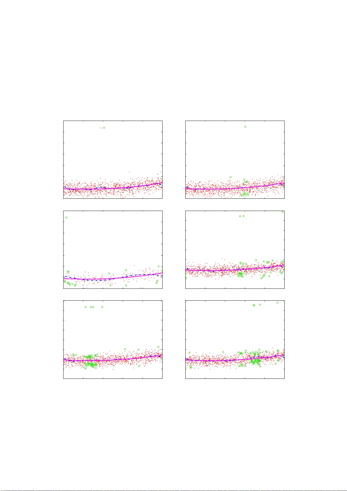
Risk bounds in linear re gre ssion through P A C-Bayesian t runcation J E A N - Y V E S A U D I B E RT 1 , 2 , O L I V I E R C A T O N I 3 Novembe r 1, 2018 A B S T R A C T : W e consi der the problem of predictin g as well as the bes t linear combi- nation of d gi ven f unctio ns in lea st squares regr ession , and va riants of this prob lem i nclud - ing constraint s on the paramete rs of the linear combinat ion. When the input distrib ution is kno wn, there already ex ists an algor ithm havin g an expe cted excess risk of order d/n , where n is the size of the training data. W ithou t this strong assumption, standard results often contain a multiplicati ve log n factor , and require some additiona l assumptio ns like unifor m boun dedne ss of t he d -dimensi onal input representa tion and expo nentia l moments of the output. This work pro vides ne w risk bounds for the rid ge estimator and the ordinary leas t square s estimator , and their varian ts. It also provide s shrinkage procedures with con ver - gence rate d/n (i.e., without the logarithmic factor) in expec tation and in de viatio ns, un- der vari ous a ssumpti ons. The k ey c ommon surprisi ng facto r of th ese results is the abse nce of exponen tial m oment condition on the output distrib ution while achiev ing expon ential de viati ons. All risk bounds are obtained through a P A C -Bayesian analys is on truncated dif ferences of loss es. Finally , we show that some of these results are not parti cular to the least squares loss, b ut can be generalize d to similar strong ly con vex loss function s. 2 0 0 0 M A T H E M A T I C S S U B J E C T C L A S S I FI C ATI O N : 62J05, 62J07. K E Y W O R D S : Linear reg ressio n, G enerali zation error , Shrinkage, P A C-Bayesian theo- rems, Risk bounds , Robus t statistics , Resistant estimator s, Gibbs posterior distrib utions , Randomize d estimator s, S tatistic al learning theory C O N T E N T S I N T R O D U C T I O N . . . . . . . . . . . . . . . . . . . . . . . . 3 O U R S TA T I S T I C A L T A S K . . . . . . . . . . . . . . . . . . . . 3 W H Y S H O U L D W E B E I N T E R E S T E D I N T H I S T A S K . . . . . . . . . . 5 O U T L I N E A N D C O N T R I B U T I O N S . . . . . . . . . . . . . . . . . 6 1 Université Paris-Est, Ecole des Ponts ParisT ech , Imagine, 6 avenue Blaise Pascal, 7 7455 Marne-la-V allée, France, audibert@imagine. enpc.fr 2 W illow , CNRS/ENS/INRIA — UMR 8548, 45 rue d’Ulm, F75230 P aris cedex 05, France 3 Départemen t de Math ématiques et Applications, CNRS – UMR 8553, École No rmale Supérieur e, 45 rue d’Ulm, F75230 Paris cedex 0 5, olivier . catoni@ens.fr 1 1 . V A R I A N T S O F K N OW N R E S U LT S . . . . . . . . . . . . . . . . 7 1 . 1 . O R D I N A RY L E A S T S Q U A R E S A N D E M P I R I C A L R I S K M I N I M I Z A - T I O N . . . . . . . . . . . . . . . . . . . . . . . . . 7 1 . 2 . P RO J E C T I O N E S T I M A T O R . . . . . . . . . . . . . . . . . . 11 1 . 3 . P E N A L I Z E D L E A S T S Q U A R E S E S T I M A T O R . . . . . . . . . . . 11 1 . 4 . C O N C L U S I O N O F T H E S U RV E Y . . . . . . . . . . . . . . . 12 2 . R I D G E R E G R E S S I O N A N D E M P I R I C A L R I S K M I N I M I Z A T I O N . . . . . 13 3 . A M I N - M A X E S T I M A T O R F O R RO B U S T E S T I M A T I O N . . . . . . . 15 3 . 1 . T H E M I N - M A X E S T I M A T O R A N D I T S T H E O R E T I C A L G U A R A N T E E . . . 15 3 . 2 . T H E V A L U E O F T H E U N C E N T E R E D K U RT O S I S C O E FFI C I E N T χ . . . . 17 3 . 3 . C O M P U T ATI O N O F T H E E S T I M A T O R . . . . . . . . . . . . . . 20 3 . 4 . S Y N T H E T I C E X P E R I M E N T S . . . . . . . . . . . . . . . . . 2 2 3.4.1. Noise dist ributions . . . . . . . . . . . . . . . . . 22 3.4.2. Independent nor malized covariates (I NC ( n, d ) ) . . . . . 23 3.4.3. Highly corr elated covariates (HCC ( n, d ) ) . . . . . . . 23 3.4.4. T rigonometr ic series (TS ( n, d ) ) . . . . . . . . . . . . 23 3.4.5. Experiments . . . . . . . . . . . . . . . . . . . 23 4 . A S I M P L E T I G H T R I S K B O U N D F O R A S O P H I S T I C A T E D P AC - B A Y E S A L G O R I T H M . . . . . . . . . . . . . . . . . . . . . 25 5 . A G E N E R I C L O C A L I Z E D P AC - B A Y E S A P P R OA C H . . . . . . . . . 27 5 . 1 . N OTA T I O N A N D S E T T I N G . . . . . . . . . . . . . . . . . . 27 5 . 2 . T H E L O C A L I Z E D P A C - B A Y E S B O U N D . . . . . . . . . . . . . 29 5 . 3 . A P P L I C A T I O N U N D E R A N E X P O N E N T I A L M O M E N T C O N D I T I O N . . . 30 5 . 4 . A P P L I C A T I O N W I T H O U T E X P O N E N T I A L M O M E N T C O N D I T I O N . . . . 32 6 . P R O O F S . . . . . . . . . . . . . . . . . . . . . . . . . . 35 6 . 1 . M A I N I D E A S O F T H E P R O O F S . . . . . . . . . . . . . . . . 35 6.1.1. Sub-exponential ta ils under a non-exponential mo ment assumption via truncatio n . . . . . . . . . . . . . . 36 6.1.2. Localized P A C-Bayesian in equalities to eliminate a log- arithm factor . . . . . . . . . . . . . . . . . . . 37 6 . 2 . P RO O F S O F T H E O R E M S 2 . 1 A N D 2 . 2 . . . . . . . . . . . . . 40 6.2.1. Pr oof of Theor em 2.1 . . . . . . . . . . . . . . . . 46 6.2.2. Pr oof of Theor em 2.2 . . . . . . . . . . . . . . . . 47 6 . 3 . P RO O F O F T H E O R E M 3 . 1 . . . . . . . . . . . . . . . . . . 50 2 6 . 4 . P RO O F O F T H E O R E M 5 . 1 . . . . . . . . . . . . . . . . . . 57 6.4.1. Pr oof of E n R exp  V 1 ( ˆ f )  ρ ( d ˆ f ) o ≤ 1 . . . . . . . . . 58 6.4.2. Pr oof of E h R exp( V 2 ) ρ ( d ˆ f ) i ≤ 1 . . . . . . . . . . . 59 6 . 5 . P RO O F O F L E M M A 5 . 3 . . . . . . . . . . . . . . . . . . 61 6 . 6 . P RO O F O F L E M M A 5 . 4 . . . . . . . . . . . . . . . . . . 62 6 . 7 . P RO O F O F L E M M A 5 . 6 . . . . . . . . . . . . . . . . . . 63 6 . 8 . P RO O F O F L E M M A 5 . 7 . . . . . . . . . . . . . . . . . . 64 A . U N I F O R M L Y B O U N D E D C O N D I T I O NA L V A R I A N C E I S N E C E S S A RY T O R E AC H d/n R A T E . . . . . . . . . . . . . . . . . . . . 64 B . E M P I R I C A L R I S K M I N I M I Z A T I O N O N A B A L L : A NA LY S I S D E - R I V E D F R O M T H E W O R K O F B I R G É A N D M A S S A RT . . . . . . . . 65 C . R I D G E R E G R E S S I O N A N A L Y S I S F RO M T H E W O R K O F C A P O N - N E T T O A N D D E V I T O . . . . . . . . . . . . . . . . . . . . 6 7 D . S O M E S TA N D A R D U P P E R B O U N D S O N L O G - L A P L A C E T R A N S - F O R M S . . . . . . . . . . . . . . . . . . . . . . . . . . 68 E . E X P E R I M E N TA L R E S U LT S F O R T H E M I N - M A X T R U N C A T E D E S - T I M A T O R D E FI N E D I N S E C T I O N 3 . 3 . . . . . . . . . . . . . . 70 I N T R O D U C T I O N O U R S T A T I S T I C A L T A S K . Let Z 1 = ( X 1 , Y 1 ) , . . . , Z n = ( X n , Y n ) be n ≥ 2 pairs of input-output and assume that each pair has bee n independently drawn from the same un known distribution P . Let X denote t he input space and let th e output sp ace be the s et of real num bers R , so t hat P is a probability di stribution on the product space Z , X × R . The target o f learning algorithms is to predict the output Y associated wit h an i nput X for pairs Z = ( X , Y ) drawn from the distribution P . The quality of a (prediction) function f : X → R is measured by the least squares risk : R ( f ) , E Z ∼ P  [ Y − f ( X )] 2  . Through t he paper , we assum e that the output and all the predict ion functions we consider are square inte grable. Let Θ b e a closed con ve x set o f R d , and ϕ 1 , . . . , ϕ d be d prediction functions. Consider the regression model F =  f θ = d X j =1 θ j ϕ j ; ( θ 1 , . . . , θ d ) ∈ Θ  . 3 The best function f ∗ in F is d eﬁned by f ∗ = d X j =1 θ ∗ j ϕ j ∈ ar gmin f ∈ F R ( f ) . Such a function always e x ists but is not necessarily unique. Besides it is unknown since the probabilit y genera ting the data is unknown. W e will study t he problem of predicting (at least) as wel l as function f ∗ . In other words, we w ant t o deduce from t he ob serva tions Z 1 , . . . , Z n a functio n ˆ f having with high probability a ri sk bou nded by the m inimal risk R ( f ∗ ) on F plus a small re mainder term, which i s typi cally of order d/n up to a possi ble logarithmi c factor . Except in particular settings (e.g., Θ is a sim plex and d ≥ √ n ), i t is known that t he con ver gence rate d/n cannot be improved in a minim ax sens e (see [20], and [21] for related results). More formally , the tar get of the paper is to de velop esti mators ˆ f for which the excess risk is cont rolled in deviations , i.e., such th at for an appropriate constant κ > 0 , for any ε > 0 , with probabili ty at least 1 − ε , R ( ˆ f ) − R ( f ∗ ) ≤ κ d + log ( ε − 1 ) n . (0.1) Note that by integrating t he de viations (using the identi ty E W = R + ∞ 0 P ( W > t ) dt which holds true for any nonnegative random variable W ), Inequality (0.1) implies E R ( ˆ f ) − R ( f ∗ ) ≤ κ d + 1 n . (0.2) In this work, we do not assume that the function f (reg) : x 7→ E [ Y | X = x ] , which m inimizes t he ri sk R am ong all poss ible measurable functions, belongs to the model F . So we mi ght ha ve f ∗ 6 = f (reg) and in this case, bounds of the form E R ( ˆ f ) − R ( f (reg) ) ≤ C [ R ( f ∗ ) − R ( f (reg) )] + κ d n , (0.3) with a const ant C larger than 1 d o no t even ensure that E R ( ˆ f ) tends to R ( f ∗ ) when n goes to inﬁnity . This kind of bou nds wit h C > 1 hav e been developed to analy ze non parametric estim ators using linear approxim ation spaces, in which case th e dimens ion d is a function of n chosen so that the bias term R ( f ∗ ) − R ( f (reg) ) has th e o rder d/n of the estimation term (see [11] and references within). Here we intend to assess the generalization ability of the esti mator e ven when the 4 model is mi sspeciﬁed (namely when R ( f ∗ ) > R ( f (reg) ) ). Moreo ver we do not assume either that Y − f (reg) ( X ) and X are independent. Notation. When Θ = R d , the function f ∗ and the space F will be written f ∗ lin and F lin to emphasize that F is the whole linear space spanned by ϕ 1 , . . . , ϕ d : F lin = span { ϕ 1 , . . . , ϕ d } and f ∗ lin ∈ ar gmin f ∈ F lin R ( f ) . The Euclidean n orm will simpl y be written as k · k , and h · , ·i will be its associated inner produ ct. W e will cons ider the vector valued functio n ϕ : X → R d deﬁned by ϕ ( X ) =  ϕ k ( X )  d k =1 , so that for any θ ∈ Θ , we hav e f θ ( X ) = h θ , ϕ ( X ) i . The Gram matrix is the d × d -matrix Q = E  ϕ ( X ) ϕ ( X ) T  , and i ts sm allest and lar gest eigen values will respectively be writ ten as q min and q max . The empirical risk of a function f is r ( f ) = 1 n n X i =1  f ( X i ) − Y i  2 and for λ ≥ 0 , the ridge regression estimator on F is deﬁned by ˆ f (ridge) = f ˆ θ (ridge) with ˆ θ (ridge) ∈ arg min θ ∈ Θ r ( f θ ) + λ k θ k 2 , where λ is some non negati ve real parameter . In the case when λ = 0 , th e ri dge regression ˆ f (ridge) is nothing but t he empirical risk minim izer ˆ f (erm) . In the same way , we i ntroduce the opt imal rid ge function optimi zing th e expected ridge risk: ˜ f = f ˜ θ with ˜ θ ∈ arg min θ ∈ Θ  R ( f θ ) + λ k θ k 2  . (0.4) Finally , let Q λ = Q + λI be t he ridge regularization of Q , where I is the identity matrix. W H Y S H O U L D W E B E I N T E R E S T E D I N T H I S T A S K . There are three main rea- sons. First we aim at a bett er understandin g of the parametric l inear least squares method (c lassical te xtbooks can be misleading on this subject as we w ill point out later), and intend to provide a non-asymptotic analysis of it. Secondly , t he task i s central in nonparametric estimati on for li near app roxima- tion s paces (piecewise polynom ials b ased on a regular partition, wav elet expan- sions, trigonomet ric polynomials. . . ) Thirdly , it naturall y arises in two-stage model selection. Precisely , when fac- ing the data, the st atistician has often to cho ose se veral model s which are likely to 5 be rele vant for the task. T hese models can be of similar structures (like embedded balls of functi onal s paces) or o n th e cont rary of very di f ferent natu re (e.g., b ased on k ernels, spli nes, wa velets or on parametric approaches). For each of t hese models, we assume that we ha ve a learning scheme which produces a ’good ’ pre- diction function in the sense that it predicts as well as the best function of the model up to some small addi tive term . Then the question is to decide on ho w we use or combi ne/aggregate t hese schemes. One possibl e answer is to spli t the data into two groups, use the ﬁrst group to train the predi ction funct ion associated with each mo del, and ﬁnally use the second group t o build a p rediction function which i s as good as (i) the best of the pre viously learnt prediction functions, (ii) the best con vex combi nation of these functi ons or (iii) the best linear com bination of these functio ns. This point of view has been intro duced by Nemirovski in [17] and optimal rates of aggregation are gi ven in [20] and references within . This pa- per focuses mo re on the linear aggregation task (eve n if (ii) enters i n our setting), assuming implicitly here t hat the m odels are gi ven in advance and are beyond our control and that the goal is to combine them appropriately . O U T L I N E A N D C O N T R I B U T I O N S . The paper i s organized as follows. Section 1 is a survey on risk bound s in li near least squares. Theorems 1.3 and 1. 5 are the results w hich come closer to our target. Section 2 provides a ne w analysis of the ridge estimato r and the ordinary least squares estimator , and their variants. Theorem 2.1 provides an asymptotic result for the ridge estimator while Theorem 2.2 gives a n on asymp totic risk boun d of the empirical risk m inimizer , which i s complementary to the t heorems put in the survey section. In particular , t he result has the beneﬁt to hold for the ordinary least squares estimator and for hea vy- tailed o utputs. W e show q uantitatively that the ridge penalty leads to an implici t reduction of the input s pace dim ension. Section 3 sh ows a non asymp totic d /n exponential de viation risk bound under weak moment conditions on the output Y and on the d -dimensional i nput representation ϕ ( X ) . Section 4 presents stronger results under boundedness assumption of ϕ ( X ) . Ho we ver the latter results are concerned with a not easily computable estim ator . Section 5 gives risk bo unds for general loss functions from which the results of Section 4 are deriv ed. The main contribution of th is paper i s to show through a P A C-Bayesian anal- ysis on truncated differ ences of los ses that the o utput distribution do es not need to have bounded conditi onal exponential mo ments i n order for t he excess ris k of appropriate estim ators to concentrate exponentially . Our results tend t o say that truncation leads to more rob us t algorithms. Local robustness t o contaminati on is usually inv oked to advoc ate the removal of outliers, claiming that esti mators should b e made insensitive to sm all amount s of spurious data. Our work leads to a different theoretical e xp lanation. The observed points ha v ing unusually large 6 outputs when compared with the (empirical) variance s hould b e down-weighted in t he estimation of the mean, since they contain less in formation than noise. In short, huge outputs should be truncated because of their low s ignal to noise ratio. 1 . V A R I A N T S O F K N OW N R E S U LT S 1 . 1 . O R D I NA RY L E A S T S Q UA R E S A N D E M P I R I C A L R I S K M I N I M I Z A T I O N . The ordinary least squares estim ator is the most standard meth od in this case. It m ini- mizes the empirical risk r ( f ) = 1 n n X i =1 [ Y i − f ( X i )] 2 , among functions in F lin and produces ˆ f (ols) = d X j =1 ˆ θ (ols) j ϕ j , with ˆ θ (ols) = [ ˆ θ (ols) j ] d j =1 a column vec tor satisfying X T X ˆ θ (ols) = X T Y , (1.1) where Y = [ Y j ] n j =1 and X = ( ϕ j ( X i )) 1 ≤ i ≤ n, 1 ≤ j ≤ d . It is well-known that • the li near system (1.1) has at least one sol ution, and in fact, the s et of so- lutions is exactly { X + Y + u ; u ∈ ke r X } ; where X + is the Moore-Penrose pseudoin verse of X and k er X is the kernel of the linear operator X . • X ˆ θ (ols) is the (unique) orth ogonal proj ection of the vector Y ∈ R n on the image of the linear map X ; • if sup x ∈ X V ar( Y | X = x ) = σ 2 < + ∞ , we h a ve (see [11, Theorem 1 1.1]) for any X 1 , . . . , X n in X , E  1 n n X i =1  ˆ f (ols) ( X i ) − f (reg) ( X i )  2     X 1 , . . . , X n  − min f ∈ F lin 1 n n X i =1  f ( X i ) − f (reg) ( X i )  2 ≤ σ 2 rank ( X ) n ≤ σ 2 d n , (1.2) where we recall th at f (reg) : x 7→ E [ Y | X = x ] i s the optimal regression function, and th at when this function belongs to F lin (i.e., f (reg) = f ∗ lin ), the minimum term in (1.2) va nishes; 7 • from Pythagoras’ theorem for the (semi)norm W 7→ √ E W 2 on the space of the square integrable random v ariabl es, R ( ˆ f (ols) ) − R ( f ∗ lin ) = E  ˆ f (ols) ( X ) − f (reg) ( X )   Z 1 , . . . , Z n  2 − E  f ∗ lin ( X ) − f (reg) ( X )  2 . (1.3) The ana lysis of the ordinary least squares often stops at this poi nt in classical statistical t extbooks. ( Besides, to simplify , the strong assumption f (reg) = f ∗ lin is often made.) This can be m isleading since Inequali ty (1.2) d oes not imply a d/n upper bound on the risk of ˆ f (ols) . Neve rtheless the follo wing result holds [11, Theorem 11.3]. T H E O R E M 1 . 1 If sup x ∈ X V ar( Y | X = x ) = σ 2 < + ∞ an d k f (reg) k ∞ = sup x ∈ X | f (reg) ( x ) | ≤ H for some H > 0 , then the truncated estimator ˆ f (ols) H = ( ˆ f (ols) ∧ H ) ∨ − H sa tisﬁes E R ( ˆ f (ols) H ) − R ( f (reg) ) ≤ 8[ R ( f ∗ lin ) − R ( f (reg) )] + κ ( σ 2 ∨ H 2 ) d log n n (1.4) for some numerical constant κ . Using P A C-Bayesian inequ alities, Catoni [8, Proposition 5.9.1] has proved a diffe rent type of results on the generalization ability of ˆ f (ols) . T H E O R E M 1 . 2 Let F ′ ⊂ F lin satisfying for some positive constants a, M , M ′ : • ther e exists f 0 ∈ F ′ s.t. for any x ∈ X , E n exp h a   Y − f 0 ( X )   i    X = x o ≤ M . • for any f 1 , f 2 ∈ F ′ , sup x ∈ X | f 1 ( x ) − f 2 ( x ) | ≤ M ′ . Let Q = E  ϕ ( X ) ϕ ( X ) T  and ˆ Q =  1 n P n i =1 ϕ ( X i ) ϕ ( X i ) T  be r esp ectively the e xpected and empirical Gram mat rices. If det Q 6 = 0 , then ther e e xist positi ve constants C 1 and C 2 (depending only on a , M and M ′ ) such that with pr obabilit y at least 1 − ε , as soon as  f ∈ F lin : r ( f ) ≤ r ( ˆ f (ols) ) + C 1 d n  ⊂ F ′ , (1.5) we have R ( ˆ f (ols) ) − R ( f ∗ lin ) ≤ C 2 d + log ( ε − 1 ) + log( det ˆ Q det Q ) n . 8 This result can be understood as follows. Let us assume we have some p rior knowledge suggesting t hat f ∗ lin belongs to the interio r of a set F ′ ⊂ F lin (e.g., a b ound on the coef ﬁcients of the expansion of f ∗ lin as a linear combination of ϕ 1 , . . . , ϕ d ). It i s likely th at (1.5 ) hol ds, and it is indeed proved in Catoni [8, section 5.11] that the probability that it does not hold goes to zero exponentially fast with n i n the case when F ′ is a Euclidean ball. If it is the case, th en we know that the e xcess r isk is of order d/n up to the unpleasant r atio of d eterminants, which, fortunately , almost surely tends to 1 as n go es to inﬁnity . By using localized P A C-Bayes i nequalities introduced in Catoni [7, 9], on e can deriv e from Inequality (6.9) and Lemma 4.1 of Alquier [1] the follo wing result. T H E O R E M 1 . 3 Let q min be the small est eigen value of the Gram matr ix Q = E  ϕ ( X ) ϕ ( X ) T  . Assume that th er e exist a function f 0 ∈ F lin and positive con- stants H and C such that k f ∗ lin − f 0 k ∞ ≤ H . and | Y | ≤ C almost surely . Then for an appr op riate r andomized estimator r equiring the knowledge of f 0 , H and C , for any ε > 0 w ith pr o bability at least 1 − ε w .r .t. the distri bution generating the observations Z 1 , . . . , Z n and the r andomized pr edictio n functio n ˆ f , we have R ( ˆ f ) − R ( f ∗ lin ) ≤ κ ( H 2 + C 2 ) d log(3 q − 1 min ) + log(( lo g n ) ε − 1 ) n , (1.6) for some κ n ot depending on d and n . Using the result of [8, Section 5 .11], one can prove that A lquier’ s result sti ll holds for ˆ f = ˆ f (ols) , but with κ also depending on t he det erminant of the prod- uct matrix Q . The lo g [log ( n )] f actor is uni mportant and could be removed in the special case quoted here (it comes from a union bound o n a grid of pos- sible temperature parameters, whereas th e t emperature could be set here t o a ﬁxed v alu e). The result differs from Theorem 1.2 essentially by the fa ct that the ratio of the determinants of the empirical and expected prod uct matrices h as been replaced by the inv erse of t he smallest eigen value of the quadratic form θ 7→ R ( P d j =1 θ j ϕ j ) − R ( f ∗ lin ) . In the case wh en the expected Gram matrix is known, (e.g., in the case of a ﬁxed design, and also in th e sligh tly different context of transdu ctiv e inference), t his s mallest eigenv alue can be s et to one b y choosi ng the quadratic form θ 7→ R ( f θ ) − R ( f ∗ lin ) to deﬁne the Euclidean m etric on the parameter space. Localized Rademacher com plexities [13, 4] allow to prove the following p rop- erty of the empirical risk minimi zer . 9 T H E O R E M 1 . 4 Assume that the input r epr esentation ϕ ( X ) , the set of parameters and the o utput Y ar e a lmost surely bounded, i.e., for some positive const ants H and C , sup θ ∈ Θ k θ k ≤ 1 ess sup k ϕ ( X ) k ≤ H , and | Y | ≤ C a.s. . Let ν 1 ≥ · · · ≥ ν d be the eigen values of the Gram matrix Q = E  ϕ ( X ) ϕ ( X ) T  . The empi rical risk minimiz er satisﬁes for any ε > 0 , with pr obability at leas t 1 − ε : R ( ˆ f (erm) ) − R ( f ∗ ) ≤ κ ( H + C ) 2 min 0 ≤ h ≤ d  h + q n ( H + C ) 2 P i>h ν i  + log ( ε − 1 ) n ≤ κ ( H + C ) 2 rank ( Q ) + log( ε − 1 ) n , wher e κ is a numerical constant . P R O O F . The resu lt i s a modiﬁed version of Theorem 6.7 in [4] applied to the linear kernel k ( u, v ) = h u, v i / ( H + C ) 2 . Its proof fol lows the same lines as in Theorem 6.7 mutatis mutan di : Corollary 5.3 and Lemm a 6.5 should be used as in termediate steps instead of Theorem 5.4 and Lemma 6.6, the nonzero eigen values of th e integral operator induced by the k ernel being the nonzero eigen values of Q .  When we kno w that th e tar get function f ∗ lin is in side so me L ∞ ball, it is natural to consider the empirical risk minimi zer on this ball. This allows to compare Theorem 1.4 to excess risk bounds with respect to f ∗ lin . Finally , from the work of Bir gé and Mass art [5], we may derive t he following risk bound for the empirical risk minim izer on a L ∞ ball (see Appendix B). T H E O R E M 1 . 5 Assume that F has a diameter H f or L ∞ -norm, i.e., for any f 1 , f 2 in F , sup x ∈ X | f 1 ( x ) − f 2 ( x ) | ≤ H and ther e exists a function f 0 ∈ F satisfying the ex ponential moment condition: for any x ∈ X , E n exp h A − 1   Y − f 0 ( X )   i    X = x o ≤ M , (1.7) for some positive constants A an d M . Let ˜ B = inf φ 1 ,...,φ d sup θ ∈ R d −{ 0 } k P d j =1 θ j φ j k 2 ∞ k θ k 2 ∞ wher e the inﬁmum is tak en with r espect to all possible or thonormal basis of F for the dot pr oduct h f 1 , f 2 i = E f 1 ( X ) f 2 ( X ) (when the set F admits no basis with 10 e xactly d functio ns, we set ˜ B = + ∞ ). Then the empiri cal risk minimizer satisﬁ es for any ε > 0 , with pr obab ility at least 1 − ε : R ( ˆ f (erm) ) − R ( f ∗ ) ≤ κ ( A 2 + H 2 ) d log [2 + ( ˜ B /n ) ∧ ( n/d )] + log ( ε − 1 ) n , wher e κ is a positi ve constant depending only on M . This result com es c loser to what we are looking for: it gi ves exponential devi- ation inequalit ies of order at worse d log( n/d ) /n . It shows that, e ven if t he Gram matrix Q has a very s mall eigen value, there is an algorithm satisfyi ng a con ver - gence rate of order d log( n/d ) /n . W it h this respect, th is result is stronger than Theorem 1.3. Howev er there are cases in which the smallest eigen value of Q is of order 1 , whi le ˜ B is large (i .e., ˜ B ≫ n ). In these cases, Theorem 1.3 does not contain the logarithmic factor which appears in Theorem 1.5. 1 . 2 . P RO J E C T I O N E S T I M A T O R . When t he input distribution is kno wn, an alter - nativ e t o the ordin ary l east squares estim ator is the following proj ection estima- tor . One ﬁrst ﬁnds an orthonormal basis of F lin for the dot product h f 1 , f 2 i = E f 1 ( X ) f 2 ( X ) , and then uses th e projection estim ator on this basis. Speciﬁcally , if φ 1 , . . . , φ d form an orthono rmal basis of F lin , t hen the projectio n esti mator on this basis is: ˆ f (proj) = d X j =1 ˆ θ (proj) j φ j , with ˆ θ (proj) = 1 n n X i =1 Y i φ j ( X i ) . Theorem 4 in [20] gives a simple bound of order d /n on the expected excess risk E R ( ˆ f (proj) ) − R ( f ∗ lin ) . 1 . 3 . P E NA L I Z E D L E A S T S Q U A R E S E S T I M A T O R . It is well establish ed that pa- rameters of the ordinary least squares estim ator are numerically unstable, and that the phenomenon can be corrected by addin g an L 2 penalty ([15, 18]). This solu- tion has been labeled ridge re gression in statistics ([12]), and consists in replacing ˆ f (ols) by ˆ f (ridge) = f ˆ θ (ridge) with ˆ θ (ridge) ∈ ar gmin θ ∈ R d  r ( f θ ) + λ d X j =1 θ 2 j  , where λ is a positive parameter . The t ypical value of λ s hould be small to av oid excessi ve s hrinkage of the coefﬁcients, b ut not t oo sm all i n order to make the optimizatio n task nu merically more stable. 11 Risk bounds for this estimator can be deri ved from general results concerning penalized least s quares on reproducing kernel Hil bert spaces ([6]), but as i t is shown in Appendix C , t his ends up wi th comp licated results having the desired d/n rate only under strong assumptions . Another popular re g ularizer is the L 1 norm. This procedure is known as Lasso [19] and is deﬁned by ˆ θ (lasso) ∈ ar gmin θ ∈ R d  r ( f θ ) + λ d X j =1 | θ j |  . As the L 2 penalty , t he L 1 penalty s hrinks the coefﬁcients. The diffe rence is that for coef ﬁcients which tend to be close to zero, the shrinkage makes them equal to zero. This all ows to select relev ant variables (i.e., ﬁnd the j ’ s such that θ ∗ j 6 = 0 ). If we assume that the regression fun ction f (reg) is a linear combination of only d ∗ ≪ d variables/functions ϕ j ’ s, the typical result is to prove that the risk of the Lasso estimato r for λ of order p (log d ) /n is of order ( d ∗ log d ) / n . Since this quantity is much smaller than d/n , this makes a huge improve ment (provided that t he sparsit y assum ption is true). This ki nd o f results usually requires stron g conditions on the eigen values of submatrices of Q , essentially ass uming th at the functions ϕ j are near orthogonal. W e do not know to whi ch extent these condit ions are required. Ho wever , i f we do no t consi der t he speciﬁc algorithm of Lasso, but the model s election approach dev eloped in [1], one can change these conditions into a single condit ion concerning on ly the minimal eigen v alue of th e subm atrix of Q corresponding to relev ant v ariables. In f act, we will see that e ven t his cond ition can be removed. 1 . 4 . C O N C L U S I O N O F T H E S U RV E Y . Previous resul ts clearly leav e room to im- provements. The projectio n estimator requires th e unrealistic assump tion that the input dist ribution is kn own, and the result holds onl y in e xp ectation. Results usi ng L 1 or L 2 regularizations require strong a ssumptio ns, in particular on the eigen val- ues of (sub matrices of) Q . Th eorem 1.1 provides a ( d log n ) / n con ver gence rate only when the R ( f ∗ lin ) − R ( f (reg) ) is at most of order ( d log n ) /n . Theorem 1.2 giv es a different type of gu arantee: the d /n is indeed achiev ed, but th e random ratio of determi nants app earing in the bound may raise some eyebrows and forbid an explicit computation of the bound and comparison w ith o ther boun ds. Theorem 1.3 seems to i ndicate that the rate of con vergence will be de graded when the Gram matrix Q is un known a nd ill-conditi oned. Theorem 1 .4 does not put any assump - tion on Q to reach the d/n rate, b ut requires particular boundedness constraints on the p arameter set, the input vector ϕ ( X ) and the outpu t. Finally , Theorem 1.5 comes closer t o what we are looking for . Y et there is sti ll an unwanted l oga- 12 rithmic factor , and the result holds only when the output has uniformly bounded conditional exponential moments, which as we will sho w is not necessary . 2 . R I D G E R E G R E S S I O N A N D E M P I R I C A L R I S K M I N I M I Z A T I O N W e recall the deﬁnition F =  f θ = d X j =1 θ j ϕ j ; ( θ 1 , . . . , θ d ) ∈ Θ  , where Θ i s a closed conv ex set, not necessarily bounded (so that Θ = R d is allowed). In this section, we provide e xponential de viation inequalities for the empirical ris k mi nimizer and the ridge re gression esti mator on F under weak con- ditions on the tail of the output distribution. The mos t general theorem which can be obtain ed from the rou te foll owed in this section is Theorem 6.5 (page 46) stated along with the p roof. It is expressed in terms o f a series of empi rical bounds. The ﬁrst deduction we can make from this technical result is of asym ptotic nature. It is stated under weak hypotheses, taking advantage of the weak law of lar ge numb ers. T H E O R E M 2 . 1 F or λ ≥ 0 , let ˜ f be its associated optimal rid ge function (see (0.4) ). Let us assu me that E  k ϕ ( X ) k 4  < + ∞ , (2.1) and E n k ϕ ( X ) k 2  ˜ f ( X ) − Y  2 o < + ∞ . (2.2) Let ν 1 , . . . , ν d be the eigen values of the G ram mat rix Q = E  ϕ ( X ) ϕ ( X ) T  , and let Q λ = Q + λI be the ridge r e gularizat ion of Q . Let us deﬁne the effecti ve ridge dimension D = d X i =1 ν i ν i + λ 1 ( ν i > 0) = T r  ( Q + λI ) − 1 Q  = E  k Q − 1 / 2 λ ϕ ( X ) k 2  . When λ = 0 , D is equal to the rank of Q and is otherwise smaller . F or any ε > 0 , ther e is n ε , such th at for any n ≥ n ε , with pr o bability at least 1 − ε , R ( ˆ f (ridge) ) + λ k ˆ θ (ridge) k 2 ≤ min θ ∈ Θ  R ( f θ ) + λ k θ k 2  + 30 E  k Q − 1 / 2 λ ϕ ( X ) k 2  ˜ f ( X ) − Y  2  E  k Q − 1 / 2 λ ϕ ( X ) k 2  D n 13 + 100 0 sup v ∈ R d E h h v , ϕ ( X ) i 2  ˜ f ( X ) − Y  2 i E ( h v , ϕ ( X ) i 2 ) + λ k v k 2 log(3 ε − 1 ) n ≤ min θ ∈ Θ  R ( f θ ) + λ k θ k 2  + ess sup E  [ Y − ˜ f ( X )] 2   X  30 D + 100 0 log(3 ε − 1 ) n P R O O F . See Section 6.2 (page 4 0).  This theorem s hows that the ordinary least squares estimator (obtained when Θ = R d and λ = 0 ), as well as the empirical risk minimizer o n any closed con vex set, asympt otically reaches a d/n speed of conv er g ence u nder very weak hypotheses. It s hows also the regularization effect of t he ridge regression. There emer ges an effective dimension D , where the ridge penalty has a t hreshold effect on the eigen values of the Gram matrix. On t he other hand, the weakness of thi s result is its asymptotic nature : n ε may be arbit rarily large u nder such weak hypotheses, and t his shows even in t he simplest c ase of the estim ation of the m ean of a real v alu ed random variable by its empirical mean (which is the case when d = 1 and ϕ ( X ) ≡ 1 ). Let us now g iv e some non asymptoti c rate under stron ger h ypotheses and for the empirical risk mini mizer (i.e., λ = 0 ). T H E O R E M 2 . 2 Let d ′ = rank ( Q ) . Ass ume that E  [ Y − f ∗ ( X )] 4  < + ∞ and B = sup f ∈ span { ϕ 1 ,...,ϕ d }−{ 0 } k f k 2 ∞ / E [ f ( X ) 2 ] < + ∞ . Consider t he (unique) empirical r isk minimizer ˆ f (erm) = f ˆ θ (erm) : x 7→ h ˆ θ (erm) , ϕ ( x ) i on F for which ˆ θ (erm) ∈ span { ϕ ( X 1 ) , . . . , ϕ ( X n ) } 4 . F o r any values of ε and n s uch that 2 /n ≤ ε ≤ 1 and n > 12 80 B 2  3 B d ′ + log (2 /ε ) + 16 B 2 d ′ 2 n  , with pr ob ability at least 1 − ε , R ( ˆ f (erm) ) − R ( f ∗ ) ≤ 1 920 B p E [ Y − f ∗ ( X )] 4 " 3 B d ′ + log (2 ε − 1 ) n +  4 B d ′ n  2 # . 4 When F = F lin , we have ˆ θ (erm) = X + Y , with X = ( ϕ j ( X i )) 1 ≤ i ≤ n, 1 ≤ j ≤ d , Y = [ Y j ] n j =1 and X + is the Moore-Pen rose pseudoin verse of X . 14 P R O O F . See Section 6.2 (page 40).  It is quite surprisin g that th e traditional ass umption of un iform bou ndedness of the conditional exponential moments of the output can be r eplaced by a simple moment condi tion for re asonable conﬁdence le vels (i.e., ε ≥ 2 /n ). For high- est conﬁdence lev els, th ings are more tricky since we need to control wi th hi gh probability a t erm of order [ r ( f ∗ ) − R ( f ∗ )] d/n (see Th eorem 6 .6). The cost to pay to get the exponential de vi ations under only a fourth-order moment c ondition on the outp ut i s the appearance of the geometrical quantit y B as a mul tiplicative factor , as opposed to Theorems 1.3 and 1.5. More precisely , from [5, Inequality (3.2)], we have B ≤ ˜ B ≤ B d , but the quant ity ˜ B appears inside a lo garithm in Theorem 1.5. Ho we ver , T heorem 1.5 i s restricted to th e empirical risk minim izer on a L ∞ ball, while the result here is valid for any closed con ve x set Θ , and in particular applies to the ordinary least squares estimator . Theorem 2.2 is still limited in at least three ways: it applies only to uniformly bounded ϕ ( X ) , the out put needs to hav e a fourth moment, and the conﬁdence lev el should be as great as ε ≥ 2 /n . These li mitation s wil l be addressed i n the next sections by considering more in volve d algorithms. 3 . A M I N - M A X E S T I M A T O R F O R RO B U S T E S T I M A T I O N 3 . 1 . T H E M I N - M A X E S T I M A T O R A N D I T S T H E O R E T I C A L G U A R A N T E E . This section provides an alternative t o the empirical risk m inimizer with non asy mp- totic exponential risk deviations of order d/ n for any conﬁdence level. Moreover , we will assume onl y a second order moment condi tion on the o utput and cover the case of unboun ded inputs, the requirement on ϕ ( X ) being only a ﬁnit e fourth order m oment. On the ot her h and, we assume t hat the set Θ of the vectors of co- ef ﬁcients is bounded. Th e computability of th e proposed estimator a nd numerical experiments are discussed at the end of the section. Let α > 0 , λ ≥ 0 , and consider the truncation function: ψ ( x ) =      − log  1 − x + x 2 / 2  0 ≤ x ≤ 1 , log(2) x ≥ 1 , − ψ ( − x ) x ≤ 0 , For an y θ, θ ′ ∈ Θ , introduce D ( θ , θ ′ ) = nαλ ( k θ k 2 − k θ ′ k 2 ) + n X i =1 ψ  α  Y i − f θ ( X i )  2 − α  Y i − f θ ′ ( X i )  2  . W e recall ˜ f = f ˜ θ with ˜ θ ∈ arg min θ ∈ Θ  R ( f θ ) + λ k θ k 2  , and the effe ctiv e ridge 15 dimension D = d X i =1 ν i ν i + λ 1 ( ν i > 0) = T r  ( Q + λI ) − 1 Q  = E  k Q − 1 / 2 λ ϕ ( X ) k 2  . Let us assume in this section that for any j ∈ { 1 , . . . , d } , E  ϕ j ( X ) 2 [ Y − ˜ f ( X )] 2  < + ∞ , (3.1) and E  ϕ 4 j ( X )  < + ∞ . (3.2) Deﬁne S = { f ∈ F lin : E [ f ( X ) 2 ] = 1 } , (3.3) σ = q E  [ Y − ˜ f ( X )] 2  = q R ( ˜ f ) , (3.4) χ = max f ∈ S p E [ f ( X ) 4 ] , (3.5) κ = q E  [ ϕ ( X ) T Q − 1 λ ϕ ( X ) ] 2  E  ϕ ( X ) T Q − 1 λ ϕ ( X )  , (3.6) κ ′ = q E  [ Y − ˜ f ( X )] 4  E  [ Y − ˜ f ( X )] 2  = q E  [ Y − ˜ f ( X )] 4  σ 2 , (3.7) T = max θ ∈ Θ ,θ ′ ∈ Θ p λ k θ − θ ′ k 2 + E [ f θ ( X ) − f θ ′ ( X )] 2 . (3.8) T H E O R E M 3 . 1 Let us as sume that (3.1) an d (3.2) hold. F or some numerical con- stants c and c ′ , for n > cκχD , by taking α = 1 2 χ  2 √ κ ′ σ + √ χT  2  1 − cκχD n  , (3.9) for any estimator f ˆ θ satisfying ˆ θ ∈ Θ a.s ., f or any ε > 0 and any λ ≥ 0 , with pr obab ility at least 1 − ε , we have R ( f ˆ θ ) + λ k ˆ θ k 2 ≤ min θ ∈ Θ  R ( f θ ) + λ k θ k 2  + 1 nα  max θ 1 ∈ Θ D ( ˆ θ , θ 1 ) − inf θ ∈ Θ max θ 1 ∈ Θ D ( θ , θ 1 )  + cκκ ′ D σ 2 n + 8 χ  log( ε − 1 ) n + c ′ κ 2 D 2 n 2  2 √ κ ′ σ + √ χT  2 1 − cκχD n . 16 P R O O F . See Section 6.3 (page 50).  By choosing an estimator such that max θ 1 ∈ Θ D ( ˆ θ , θ 1 ) < inf θ ∈ Θ max θ 1 ∈ Θ D ( θ , θ 1 ) + σ 2 D n , Theorem 3.1 provides a non as ymptotic bound for the excess (ridge) risk with a D /n conv ergence rate and an e xponential t ail e ven wh en neither the output Y nor the i nput vector ϕ ( X ) has exponential m oments. This stronger non asym ptotic bound com pared to the bounds of t he previous s ection comes at th e price of re- placing the empiri cal ris k minim izer by a more in volved estimator . Section 3.3 provides a w ay of computing it approximately . 3 . 2 . T H E V A L U E O F T H E U N C E N T E R E D K U RT O S I S C O E FFI C I E N T χ . Let us discuss here the value of constant χ , whi ch plays a critical role in th e speed of con ver gence of our bound. W i th the con vention 0 0 = 0 , we have χ = sup u ∈ R d E  h u, ϕ ( X ) i 4  1 / 2 E  h u, ϕ ( X ) i 2  . Let us ﬁrst examine the case when ϕ 1 ( X ) ≡ 1 and  ϕ j ( X ) , j = 2 , . . . , d  are independent. T o compute χ , we can assu me without loss of generality t hat they are centered and o f unit variance, which wi ll be the case after Q − 1 / 2 is applied t o them. In this situat ion, introducing χ ∗ = max j =1 ,...,d E  ϕ j ( X ) 4  1 / 2 E  ϕ j ( X ) 2  , we see that for any u ∈ R d with k u k = 1 , we hav e E  h u, ϕ ( X ) i 4  = d X i =1 u 4 i E ( ϕ i ( X ) 4 ) + 6 X 1 ≤ i 0 and W i ( f , f ′ ) = λ  Y i − f ( X i )  2 −  Y i − f ′ ( X i )  2  . Introduce ˆ E ( f ) = lo g Z π ( d f ′ ) Q n i =1 [1 − W i ( f , f ′ ) + 1 2 W i ( f , f ′ ) 2 ] . (4.1) W e consider the “posterior” distribution ˆ π on the set F w ith density: d ˆ π dπ ( f ) = exp[ − ˆ E ( f ) ] R exp[ − ˆ E ( f ′ )] π ( d f ′ ) . (4.2) T o un derstand in tuitively wh y thi s dis tribution concentrates on functions with low risk, one shou ld t hink that when λ is s mall eno ugh, 1 − W i ( f , f ′ ) + 1 2 W i ( f , f ′ ) 2 is close to e − W i ( f ,f ′ ) , and consequently ˆ E ( f ) ≈ λ n X i =1 [ Y i − f ( X i )] 2 + log Z π ( d f ′ ) exp n − λ n X i =1  Y i − f ′ ( X i )  2 o , and d ˆ π dπ ( f ) ≈ exp {− λ P n i =1 [ Y i − f ( X i )] 2 } R exp {− λ P n i =1 [ Y i − f ′ ( X i )] 2 } π ( d f ′ ) . The following theorem g iv es a d/n con vergence rate for the random ized algo rithm which draws the prediction function from F according to the distribution ˆ π . T H E O R E M 4 . 1 Assume that F has a diameter H for L ∞ -norm: sup f 1 ,f 2 ∈ F , x ∈ X | f 1 ( x ) − f 2 ( x ) | = H (4.3) and that, for some σ > 0 , sup x ∈ X E  [ Y − f ∗ ( X )] 2   X = x  ≤ σ 2 < + ∞ . (4.4) 25 Let ˆ f be a prediction function drawn fr om the distri bution ˆ π deﬁned in (4.2, page 25) and depending on t he parameter λ > 0 . Then fo r any 0 < η ′ < 1 − λ (2 σ + H ) 2 and ε > 0 , with pr obab ility (with r espect to the distr ibution P ⊗ n ˆ π generating the observations Z 1 , . . . , Z n and the randomized prediction function ˆ f ) at least 1 − ε , we have R ( ˆ f ) − R ( f ∗ ) ≤ (2 σ + H ) 2 C 1 d + C 2 log(2 ε − 1 ) n with C 1 = log( (1+ η ) 2 η ′ (1 − η ) ) η (1 − η − η ′ ) and C 2 = 2 η (1 − η − η ′ ) and η = λ (2 σ + H ) 2 . In particular for λ = 0 . 32(2 σ + H ) − 2 and η ′ = 0 . 1 8 , we get R ( ˆ f ) − R ( f ∗ ) ≤ (2 σ + H ) 2 16 . 6 d + 12 . 5 log(2 ε − 1 ) n . Besides if f ∗ ∈ ar gmin f ∈ F lin R ( f ) , then with pr o bability at least 1 − ε , we have R ( ˆ f ) − R ( f ∗ ) ≤ (2 σ + H ) 2 8 . 3 d + 12 . 5 log(2 ε − 1 ) n . P R O O F . This is a direct consequence of Theorem 5.5 (page 33), Lemma 5.3 (page 31) and Lemma 5.6 (page 35).  If we know th at f ∗ lin belongs to some bou nded ball in F lin , then on e can deﬁne a bounded F as this ball, us e the previous theorem and obtain an excess risk bou nd with respect to f ∗ lin . R E M A R K 4 . 1 Let us discuss t his result. On the positive side, we ha ve a d/n con- ver gence rate in expectation and i n deviations. It has no extra logarithmic factor . It does not require any particul ar assumption on the smallest eigen value of the cov ariance matrix. T o achieve exponential de viations, a unifo rmly bounded sec- ond m oment of the output knowing the inpu t is s urprisingly sufﬁcient: we do no t require the traditional exponential m oment condition on the ou tput. Appendix A (page 64) ar gues that the uniformly bounded conditional second moment assump- tion cannot be replaced with just a bounded second moment condition. On the negative side, th e estimator is rather compl icated. When the target is to predict as well as t he best linear combination f ∗ lin up to a small additive t erm, it requires t he knowledge of a L ∞ -bounded ball in whi ch f ∗ lin lies and an upp er bound on sup x ∈ X E  [ Y − f ∗ lin ( X )] 2   X = x  . The loos er t his knowledge is, the bigger the constant in front of d/n is. Finally , we propose a randomized algorithm consist ing in drawing the pre- diction functio n according to ˆ π . As usu al, by con vexity of the loss function, 26 the ris k o f the deterministic estim ator ˆ f determ = R f ˆ π ( d f ) satisﬁes R ( ˆ f determ ) ≤ R R ( f ) ˆ π ( d f ) , so that, after some pretty st andard comput ations, one can prove t hat for any ε > 0 , with probabili ty at least 1 − ε : R ( ˆ f determ ) − R ( f ∗ lin ) ≤ κ (2 σ + H ) 2 d + log ( ε − 1 ) n , for some appropriate numerical constant κ > 0 . R E M A R K 4 . 2 The previous result wa s expressing boundedness in terms of th e L ∞ diameter of t he set of function s F . By using Lemma 5.7 (page 35) instead of Lemma 5 .6 (page 35), Th eorem 4.1 still hol ds without assum ing (4.3) and (4.4), but by re placing (2 σ + H ) 2 by V =  2 r sup f ∈ F lin : E [ f ( X ) 2 ]=1 E  f 2 ( X )[ Y − f ∗ ( X )] 2  + r sup f ′ ,f ′′ ∈ F E  [ f ′ ( X ) − f ′′ ( X )] 2  r sup f ∈ F lin : E [ f ( X ) 2 ]=1 E  f 4 ( X )   2 . The quantity V is ﬁnite when simultaneously , Θ is boun ded, and for any j in { 1 , . . . , d } , the quantiti es E  ϕ 4 j ( X )  and E  ϕ j ( X ) 2 [ Y − f ∗ ( X )] 2  are ﬁnite. 5 . A G E N E R I C L O C A L I Z E D P AC - B AY E S A P P R O AC H 5 . 1 . N OTA T I O N A N D S E T T I N G . In t his section, we drop the restricti ons o f the linear least sq uares settin g consi dered in the other section s in order t o focus on the ideas underlying the esti mator and the results presented i n Section 4. T o do t his, we cons ider that the lo ss incurred by predicting y ′ while the correct output is y i s ˜ ℓ ( y , y ′ ) (and is not n ecessarily equal to ( y − y ′ ) 2 ). The qualit y of a (prediction) function f : X → R is measured by its risk R ( f ) = E  ˜ ℓ  Y , f ( X )  . W e sti ll cons ider the prob lem of predi cting (at l east) as well as the best function in a gi ven set of functio ns F (but F is not necessarily a subset of a ﬁnite dimensional linear space). Let f ∗ still denot e a fun ction m inimizin g the risk among functions in F : f ∗ ∈ argmin f ∈ F R ( f ) . F or simpli city , we assume that i t exists. The excess risk is deﬁned by ¯ R ( f ) = R ( f ) − R ( f ∗ ) . 27 Let ℓ : Z × F × F → R be a function s uch that ℓ ( Z , f , f ′ ) represents 5 how worse f predicts t han f ′ on the data Z . Let us in troduce the real-v alued ran- dom processes L : ( f , f ′ ) 7→ ℓ ( Z , f , f ′ ) and L i : ( f , f ′ ) 7→ ℓ ( Z i , f , f ′ ) , where Z , Z 1 , . . . , Z n denote i.i.d. random variables with distribution P . Let π and π ∗ be two (prior) probabi lity di stributions on F . W e assume the following in tegrability condition. Condition I. F or any f ∈ F , we ha ve Z E  exp[ L ( f , f ′ )]  n π ∗ ( d f ′ ) < + ∞ , (5.1) and Z π ( d f ) R E  exp[ L ( f , f ′ )]  n π ∗ ( d f ′ ) < + ∞ . (5.2) W e consider the real-v alued processes ˆ L ( f , f ′ ) = n X i =1 L i ( f , f ′ ) , (5.3) ˆ E ( f ) = lo g Z exp[ ˆ L ( f , f ′ )] π ∗ ( d f ′ ) , (5.4) L ♭ ( f , f ′ ) = − n log  E  exp[ − L ( f , f ′ )]  , (5.5) L ♯ ( f , f ′ ) = n log  E  exp[ L ( f , f ′ )]  , (5.6) and E ♯ ( f ) = log n R exp  L ♯ ( f , f ′ )  π ∗ ( d f ′ ) o . (5.7) Essentially , t he quantities ˆ L ( f , f ′ ) , L ♭ ( f , f ′ ) and L ♯ ( f , f ′ ) represent how worse is the predictio n from f than from f ′ with respect to the t raining data or in expecta- tion. By Jensen’ s inequality , we ha ve L ♭ ≤ n E ( L ) = E ( ˆ L ) ≤ L ♯ . (5.8) The quantit ies ˆ E ( f ) and E ♯ ( f ) should be und erstood as s ome kind of (empirical or expected) excess risk of t he p rediction funct ion f with respect to an impl icit reference induced by the integral ov er F . For a di stribution ρ on F absolutely cont inuous w .r .t. π , let dρ dπ denote the density of ρ w .r .t. π . For any real-valued (measurable) functio n h deﬁned o n F 5 While the natu ral c hoice in the le ast squares setting is ℓ (( X, Y ) , f , f ′ ) = [ Y − f ( X )] 2 − [ Y − f ′ ( X )] 2 , we will see that for h eavy-tailed outputs, it is prefer able to consider the following soft-trunc ated version of it, up to a scaling f actor λ > 0 : ℓ (( X , Y ) , f , f ′ ) = T  λ  ( Y − f ( X )) 2 − ( Y − f ′ ( X )) 2  , with T ( x ) = − log(1 − x + x 2 / 2) . E quality (5.4, page 28) corresponds to (4.1, page 25) with this choice of func tion ℓ and for the choice π ∗ = π . 28 such that R exp[ h ( f )] π ( d f ) < + ∞ , we deﬁne the distribution π h on F b y its density: dπ h dπ ( f ) = exp[ h ( f )] R exp[ h ( f ′ )] π ( d f ′ ) . (5.9) W e will use the posterior distribution: d ˆ π dπ ( f ) = dπ − ˆ E dπ ( f ) = exp[ − ˆ E ( f )] R exp[ − ˆ E ( f ′ )] π ( d f ′ ) . (5.10) Finally , for any β ≥ 0 , we will us e the following measures of the s ize (or com - plexity) of F around the target function: I ∗ ( β ) = − log n R exp  − β ¯ R ( f )  π ∗ ( d f ) o and I ( β ) = − log n R exp  − β ¯ R ( f )  π ( d f ) o . 5 . 2 . T H E L O C A L I Z E D P AC - B A Y E S B O U N D . W i th the notati on introduced in the previous section, we have the following risk bound for any randomized esti- mator . T H E O R E M 5 . 1 Assume that π , π ∗ , F and ℓ satisfy the inte grability conditio ns (5.1) and (5.2, page 28) . Let ρ be a (posterior ) pr oba bility dis tribution on F ad- mitting a density with r espect to π depending on Z 1 , . . . , Z n . Let ˆ f be a pr ediction function drawn fr om t he dis tribution ρ . Then for any γ ≥ 0 , γ ∗ ≥ 0 and ε > 0 , with pr obabil ity (with r espect to t he distribution P ⊗ n ρ ge nerating the observa- tions Z 1 , . . . , Z n and the randomized pr ediction function ˆ f ) at least 1 − ε : Z  L ♭ ( ˆ f , f ) + γ ∗ ¯ R ( f )  π ∗ − γ ∗ ¯ R ( d f ) − γ ¯ R  ˆ f  ≤ I ∗ ( γ ∗ ) − I ( γ ) − log n R exp  − E ♯ ( f )  π ( d f ) o + log h dρ d ˆ π  ˆ f  i + 2 log(2 ε − 1 ) . (5.11) P R O O F . See Section 6.4 (page 57).  Some extra work will be needed to prove that Inequality (5.11) provides an upper bound on the e xcess risk ¯ R ( ˆ f ) of the estimator ˆ f . As we will s ee in the n ext sections, desp ite the − γ ¯ R ( ˆ f ) term and provided that γ i s sufﬁciently small, the lefthand-side will be essentially lower bou nded by λ ¯ R ( ˆ f ) with λ > 0 , whil e, by choosing ρ = ˆ π , the est imator does not appear in the righthand-side. 29 5 . 3 . A P P L I C A T I O N U N D E R A N E X P O N E N T I A L M O M E N T C O N D I T I O N . The es- timator proposed in Section 4 and Theorem 5.1 seems rather unnatural (or at least complicated) at ﬁrst sight . The goal of t his s ection is twofold. First it shows that under exponential moment conditions (i.e., strong er assumptions than the ones in Theorem 4.1 when the linear least square setting i s consid ered), one can have a much simpl er estim ator than t he one consi sting in dra wi ng a function according to the dis tribution (4.2 ) with ˆ E given by (4.1) and yet still obtain a d /n con ver gence rate. Secondly it illus trates Theorem 5.1 in a di f ferent and simp ler way th an the one we will use to prove Theorem 4. 1. In this section, we consider the following variance and complexity assu mp- tions. Condition V1. There exist λ > 0 and 0 < η < 1 such that for any function f ∈ F , we ha ve E n exp  λ ˜ ℓ  Y , f ( X )  o < + ∞ , log n E n exp n λ h ˜ ℓ  Y , f ( X )  − ˜ ℓ  Y , f ∗ ( X )  iooo ≤ λ (1 + η )[ R ( f ) − R ( f ∗ )] , and log n E n exp n − λ h ˜ ℓ  Y , f ( X )  − ˜ ℓ  Y , f ∗ ( X )  iooo ≤ − λ (1 − η )[ R ( f ) − R ( f ∗ )] . Condition C. There exist a probabilit y distribution π , and constants D > 0 and G > 0 such that for any 0 < α < β , log  R exp {− α [ R ( f ) − R ( f ∗ )] } π ( d f ) R exp {− β [ R ( f ) − R ( f ∗ )] } π ( d f )  ≤ D log  Gβ α  . T H E O R E M 5 . 2 Assume that V1 an d C ar e satisﬁed. Let ˆ π (Gibbs) be the pr obability distribution on F deﬁned by its density d ˆ π (Gibbs) dπ ( f ) = exp {− λ P n i =1 ˜ ℓ [ Y i , f ( X i )] } R exp {− λ P n i =1 ˜ ℓ [ Y i , f ′ ( X i )] } π ( d f ′ ) , wher e λ > 0 and the dis tribution π are those appearing r espectively i n V1 and C . Let ˆ f ∈ F be a functi on drawn acc or ding to th is Gibbs distribution. Then for any η ′ such that 0 < η ′ < 1 − η (wher e η is the cons tant appeari ng i n V1 ) and any ε > 0 , with pr obab ility at least 1 − ε , we have R ( ˆ f ) − R ( f ∗ ) ≤ C ′ 1 D + C ′ 2 log(2 ε − 1 ) n with C ′ 1 = log( G (1+ η ) η ′ ) λ (1 − η − η ′ ) and C ′ 2 = 2 λ (1 − η − η ′ ) . 30 P R O O F . W e consider ℓ  ( X , Y ) , f , f ′  = λ  ˜ ℓ  Y , f ( X )  − ˜ ℓ  Y , f ′ ( X )  , where λ i s the const ant appearing in the variance assum ption. Let us take γ ∗ = 0 and let π ∗ be t he Dirac distribution at f ∗ : π ∗ ( { f ∗ } ) = 1 . Then Condition V1 implies Condition I (page 28) and we can apply Theorem 5.1. W e hav e L ( f , f ′ ) = λ  ˜ ℓ  Y , f ( X )  − ˜ ℓ  Y , f ′ ( X )  , ˆ E ( f ) = λ n X i =1 ˜ ℓ  Y i , f ( X i )  − λ n X i =1 ˜ ℓ  Y i , f ∗ ( X i )  , ˆ π = ˆ π (Gibbs) , L ♭ ( f ) = − n log n E h exp  − L ( f , f ∗ )  io , E ♯ ( f ) = n log n E h exp  L ( f , f ∗ )  io and Assumpti on V1 lea ds to: log n E h exp  L ( f , f ∗ )  io ≤ λ (1 + η )[ R ( f ) − R ( f ∗ )] and log n E h exp  − L ( f , f ∗ )  io ≤ − λ (1 − η )[ R ( f ) − R ( f ∗ )] . Thus choosing ρ = ˆ π , (5.11) giv es [ λn (1 − η ) − γ ] ¯ R ( ˆ f ) ≤ − I ( γ ) + I  λn (1 + η )  + 2 log(2 ε − 1 ) . Accordingly by the complexity assumption, for γ ≤ λ n (1 + η ) , we get [ λn (1 − η ) − γ ] ¯ R ( ˆ f ) ≤ D log  Gλn (1 + η ) γ  + 2 log(2 ε − 1 ) , which impli es the announced r esult.  Let us conclude thi s section by mentionin g settings in wh ich assum ptions V1 and C are satisﬁed. L E M M A 5 . 3 Let Θ be a bounded con vex set of R d , and ϕ 1 , . . . , ϕ d be d square inte grable pr ediction functio ns. As sume that F =  f θ = d X j =1 θ j ϕ j ; ( θ 1 , . . . , θ d ) ∈ Θ  , π is the unifo rm distribution on F (i.e., the one coming fr om the uniform distribu- tion on Θ ), and that th er e exist 0 < b 1 ≤ b 2 such that for any y ∈ R , the f unction ˜ ℓ y : y ′ 7→ ˜ ℓ ( y , y ′ ) a dmits a second derivative satisfying: for any y ′ ∈ R , b 1 ≤ ˜ ℓ ′′ y ( y ′ ) ≤ b 2 . 31 Then Condition C holds for the above uniform π , G = p b 2 /b 1 and D = d . Besides when f ∗ = f ∗ lin (i.e., min F R = min θ ∈ R d R ( f θ ) ), Condi tion C holds for the above uniform π , G = b 2 /b 1 and D = d/ 2 . P R O O F . See Section 6.5 (page 61).  R E M A R K 5 . 1 In particular , for the least squ ares loss ˜ ℓ ( y , y ′ ) = ( y − y ′ ) 2 , we have b 1 = b 2 = 2 s o that condit ion C holds with π the uniform distribution on F , D = d and G = 1 , and with D = d/ 2 and G = 1 when f ∗ = f ∗ lin . L E M M A 5 . 4 As sume th at ther e exist 0 < b 1 ≤ b 2 , A > 0 and M > 0 such that for an y y ∈ R , the functi ons ˜ ℓ y : y ′ 7→ ˜ ℓ ( y , y ′ ) ar e twice differ entiable and satisfy: for any y ′ ∈ R , b 1 ≤ ˜ ℓ ′′ y ( y ′ ) ≤ b 2 , (5.12) and for any x ∈ X , E n exp h A − 1   ˜ ℓ ′ Y [ f ∗ ( X )]   i    X = x o ≤ M . (5.13) Assume that F is con vex and has a diameter H for L ∞ -norm: sup f 1 ,f 2 ∈ F , x ∈ X | f 1 ( x ) − f 2 ( x ) | = H. In this case Condition V1 holds for any ( λ, η ) such that η ≥ λA 2 2 b 1 exp h M 2 exp  H b 2 / A  i . and 0 < λ ≤ (2 AH ) − 1 is small enough to ensur e η < 1 . P R O O F . See Section 6.6 (page 62).  5 . 4 . A P P L I C A T I O N W I T H O U T E X P O N E N T I A L M O M E N T C O N D I T I O N . When we do not have ﬁnite exponential moments as assu med by Condition V1 (page 30), e.g., when E  exp  λ  ˜ ℓ [ Y , f ( X )] − ˜ ℓ [ Y , f ∗ ( X )]  = + ∞ for any λ > 0 and some function f in F , we cannot apply Theorem 5.1 with ℓ  ( X , Y ) , f , f ′  = λ  ˜ ℓ  Y , f ( X )  − ˜ ℓ  Y , f ′ ( X )  (because of the E ♯ term). Ho wever , we can ap- ply it to the soft truncated excess loss ℓ  ( X , Y ) , f , f ′  = T  λ  ˜ ℓ  Y , f ( X )  − ˜ ℓ  Y , f ′ ( X )   , with T ( x ) = − log (1 − x + x 2 / 2) . This section provides a result simi lar t o Theorem 5.2 in which conditio n V1 is re placed by the following condi tion. Condition V2. For any functi on f , the random variable ˜ ℓ  Y , f ( X )  − ˜ ℓ  Y , f ∗ ( X )  is square integrable and there e xists V > 0 such that for any function f , E nh ˜ ℓ  Y , f ( X )  − ˜ ℓ  Y , f ∗ ( X )  i 2 o ≤ V [ R ( f ) − R ( f ∗ )] . 32 T H E O R E M 5 . 5 Assume tha t Condi tions V2 above and C (page 30) ar e sati sﬁed. Let 0 < λ < V − 1 and ℓ  ( X , Y ) , f , f ′  = T  λ  ˜ ℓ  Y , f ( X )  − ˜ ℓ  Y , f ′ ( X )   , (5.14) with T ( x ) = − log(1 − x + x 2 / 2) . (5.15) Let ˆ f ∈ F be a fu nction drawn accor ding to the distribution ˆ π deﬁned in (5.10, page 29) with ˆ E deﬁned in (5.4, page 28) and π ∗ = π the di stribution app earing in Condit ion C . Then for any 0 < η ′ < 1 − λV and ε > 0 , with pr oba bility at least 1 − ε , we have R ( ˆ f ) − R ( f ∗ ) ≤ V C ′ 1 D + C ′ 2 log(2 ε − 1 ) n with C ′ 1 = log( G (1+ η ) 2 η ′ (1 − η ) ) η (1 − η − η ′ ) and C ′ 2 = 2 η (1 − η − η ′ ) and η = λV . In particular , for λ = 0 . 3 2 V − 1 and η ′ = 0 . 1 8 , we get R ( ˆ f ) − R ( f ∗ ) ≤ V 16 . 6 D + 12 . 5 log(2 √ Gε − 1 ) n . P R O O F . W e apply Theorem 5.1 for ℓ giv en by (5.14) and π ∗ = π . Let W ( f , f ′ ) = λ  ˜ ℓ  Y , f ( X )  − ˜ ℓ  Y , f ′ ( X )  for any f , f ′ ∈ F . Since log u ≤ u − 1 for any u > 0 , we ha ve L ♭ = − n lo g E (1 − W + W 2 / 2) ≥ n ( E W − E W 2 / 2) . Moreover , from Assum ption V2, E W ( f , f ′ ) 2 2 ≤ E W ( f , f ∗ ) 2 + E W ( f ′ , f ∗ ) 2 ≤ λ 2 V ¯ R ( f ) + λ 2 V ¯ R ( f ′ ) , (5.1 6) hence, by introducing η = λV , L ♭ ( f , f ′ ) ≥ λn  ¯ R ( f ) − ¯ R ( f ′ ) − λV ¯ R ( f ) − λV ¯ R ( f ′ )  = λn  (1 − η ) ¯ R ( f ) − (1 + η ) ¯ R ( f ′ )  . (5.17) 33 Noting that exp  T ( u )  = 1 1 − u + u 2 / 2 = 1 + u + u 2 2  1 + u 2 2  2 − u 2 = 1 + u + u 2 2 1 + u 4 4 ≤ 1 + u + u 2 2 , we see that L ♯ = n log n E h exp  T ( W )  io ≤ n  E  W  + E  W 2  / 2  . Using (5.16) and still η = λV , we get L ♯ ( f , f ′ ) ≤ λn  ¯ R ( f ) − ¯ R ( f ′ ) + η ¯ R ( f ) + η ¯ R ( f ′ )  = λn (1 + η ) ¯ R ( f ) − λn (1 − η ) ¯ R ( f ′ ) , and E ♯ ( f ) ≤ λ n (1 + η ) ¯ R ( f ) − I ( λn (1 − η )) . (5.18) Plugging (5.17) and (5.18) in (5.11) for ρ = ˆ π , we obtain [ λn (1 − η ) − γ ] ¯ R ( ˆ f ) + [ γ ∗ − λn (1 + η )] R ¯ R ( f ) π − γ ∗ ¯ R ( d f ) ≤ I ( γ ∗ ) − I ( γ ) + I ( λn (1 + η )) − I ( λn (1 − η )) + 2 lo g(2 ε − 1 ) . By the complexity a ssumption , choosi ng γ ∗ = λn (1 + η ) and γ < λn (1 − η ) , we get [ λn (1 − η ) − γ ] ¯ R ( ˆ f ) ≤ D log  G λn (1 + η ) 2 γ (1 − η )  + 2 log(2 ε − 1 ) , hence the desired result by considering γ = λnη ′ with η ′ < 1 − η .  R E M A R K 5 . 2 The estimator s eems abnormally complicated at ﬁrst sight . This remark aims at explaining why we we re not able to consider a simpler estimato r . In Section 5.3, i n which we con sider the exponential mom ent condition V1, we took ℓ  ( X , Y ) , f , f ′  = λ  ˜ ℓ  Y , f ( X )  − ˜ ℓ  Y , f ′ ( X )  and π ∗ as the Dirac distribution at f ∗ . For these choices, one can easil y check th at ˆ π does n ot depend on f ∗ . In t he absence of an e xponential m oment condition, we cannot consi der t he function ℓ  ( X , Y ) , f , f ′  = λ  ˜ ℓ  Y , f ( X )  − ˜ ℓ  Y , f ′ ( X )  but a truncated version of it. The truncation functi on T we use in Theorem 5.5 can be replaced by the simpler function u 7→ ( u ∨ − M ) ∧ M for some appropriate constant M > 0 but t his would lead to a bound with worse constants, wi thout really simp lifying the algori thm. The precise choice T ( x ) = − lo g (1 − x + x 2 / 2) comes from the remarkable property: th ere exist second order polynomial P ♭ and P ♯ such that 1 P ♭ ( u ) ≤ exp  T ( u )  ≤ P ♯ ( u ) and P ♭ ( u ) P ♯ ( u ) ≤ 1 + O ( u 4 ) for u → 0 , w hich are 34 reasonable properties to ask in order to ensure t hat (5.8 ), and consequentl y (5.11), are tight. Besides, i f we take ℓ as in (5.14 ) with T a truncation function and π ∗ as the Dirac distribution at f ∗ , then ˆ π would depend on f ∗ , and is con sequently not observable. This i s the reason why we do no t consi der π ∗ as the Dirac dis tribution at f ∗ , but π ∗ = π . This lead to the estimato r c onsidered in Theorems 5.5 and 4.1. R E M A R K 5 . 3 Theorem 5.5 still holds for the same random ized est imator in which (5.15, page 33) is replaced with T ( x ) = lo g (1 + x + x 2 / 2) . Condition V2 holds under weak assumptions as illustrated by the fol lowing lemma. L E M M A 5 . 6 Consi der the l east squar es setting: ˜ ℓ ( y , y ′ ) = ( y − y ′ ) 2 . Assume that F is con vex and has a diameter H for L ∞ -norm: sup f 1 ,f 2 ∈ F , x ∈ X | f 1 ( x ) − f 2 ( x ) | = H and that for some σ > 0 , we have sup x ∈ X E  [ Y − f ∗ ( X )] 2   X = x  ≤ σ 2 < + ∞ . (5.19) Then Condition V2 holds for V = (2 σ + H ) 2 . P R O O F . See Section 6.7 (page 63).  L E M M A 5 . 7 Consi der the l east squar es setting: ˜ ℓ ( y , y ′ ) = ( y − y ′ ) 2 . Assume that F (i.e., Θ ) is bounded, and that for any j ∈ { 1 , . . . , d } , we have E  ϕ 4 j ( X )  < + ∞ and E  ϕ j ( X ) 2 [ Y − f ∗ ( X )] 2  < + ∞ . Then Conditio n V2 holds for V =  2 r sup f ∈ F lin : E [ f ( X ) 2 ]=1 E  f 2 ( X )[ Y − f ∗ ( X )] 2  + r sup f ′ ,f ′′ ∈ F E  [ f ′ ( X ) − f ′′ ( X )] 2  r sup f ∈ F lin : E [ f ( X ) 2 ]=1 E  f 4 ( X )   2 . P R O O F . See Section 6.8 (page 64).  6 . P RO O F S 6 . 1 . M A I N I D E A S O F T H E P R O O F S . The goal of this section is t o explain the key ingredients appearing in the proofs wh ich both allows to obtain sub-exponential tails for the excess risk under a non-exponential moment assumption and get rid of the logarithmi c f actor in the excess risk bound. 35 6.1.1. S ub-ex ponential tails under a non-exponential moment a ssumption via trun- cation. Let us start with the idea allowing us to prove exponential in equalities under j ust a moment assumption (i nstead of t he traditional exponential mom ent assumption ). T o understand it, we can consider the (apparently) simplisti c 1 - dimensional situation i n whi ch we have Θ = R and the marginal distribution o f ϕ 1 ( X ) is the Dirac distri bution at 1 . In this case, t he risk o f the predicti on functi on f θ is R ( f θ ) = E ( Y − θ ) 2 = E ( Y − θ ∗ ) 2 + ( E Y − θ ) 2 , so that the least s quares r e- gression problem boils down to th e estimation of the mean of the output v ariable. If we only assume t hat Y admits a ﬁnite second m oment, say E Y 2 ≤ 1 , it is not clear whether for any ε > 0 , it is possi ble to ﬁnd ˆ θ such t hat wit h probabi lity at least 1 − 2 ε , R ( f ˆ θ ) − R ( f ∗ ) = ( E ( Y ) − ˆ θ ) 2 ≤ c log( ε − 1 ) n , (6.1) for some n umerical const ant c . Indeed, from Chebyshev’ s in equality , t he t rivial choice ˆ θ = P n i =1 Y i n just satisﬁes: with probabilit y at least 1 − 2 ε , R ( f ˆ θ ) − R ( f ∗ ) ≤ 1 nε , which is far from the ob jectiv e (6.1) for small conﬁdence levels (consider ε = exp( − √ n ) for instance). The key id ea is thus to av erage (soft) truncated values of the outputs. This is performed by taking ˆ θ = 1 nλ n X i =1 log  1 + λY i + λ 2 Y 2 i 2  , with λ = q 2 log( ε − 1 ) n . Since we hav e log E exp( nλ ˆ θ ) = n log  1 + λ E ( Y ) + λ 2 2 E ( Y 2 )  ≤ nλ E ( Y ) + n λ 2 2 , the exponential Chebyshe v’ s inequali ty (see Lem ma 6.10) guarantees that with probability at least 1 − ε , we hav e nλ ( ˆ θ − E ( Y )) ≤ n λ 2 2 + log ( ε − 1 ) , hence ˆ θ − E ( Y ) ≤ r 2 log ( ε − 1 ) n . Replacing Y by − Y in the previous argument, we o btain that with p robability at least 1 − ε , we have nλ  E ( Y ) + 1 nλ n X i =1 log  1 − λY i + λ 2 Y 2 i 2  ≤ n λ 2 2 + log ( ε − 1 ) . 36 Since − log (1 + x + x 2 / 2) ≤ lo g(1 − x + x 2 / 2) , t his implies E ( Y ) − ˆ θ ≤ q 2 log( ε − 1 ) n . The two previous i nequalities imply Inequali ty (6.1) (for c = 2 ), showing that sub-exponential tails are achieva ble even when we onl y assume that the random var iable admits a ﬁnite second m oment (see [10] for more details on the robust estimation of the mean of a random variable). 6.1.2. Locali zed P AC -Bayesian inequalit ies to eliminate a logarithm f actor. High le vel description of the P A C-Bayesian appr oach and the localization ar - gument. The a nalysis of statistical inference generally re lies on upper bounding the supremum of an empirical process χ ind exe d by the functions in a model F . One central to ol t o obtain these bounds is the concentration inequali ties. An al- ternativ e approach, called the P AC -Bayesian one, consists in using the entrop ic equality E exp sup ρ ∈ M  Z ρ ( d f ) χ ( f ) − K ( ρ, π ′ )  ! = Z π ′ ( d f ) E exp  χ ( f )  . (6.2) where M is the set of probability distributions on F and K ( ρ, π ′ ) is the Kullback- Leibler div ergence (whose deﬁnition is recalled in (6.29)) between ρ and some ﬁxed distribution π ′ . Let ˇ r : F → R be an observable process such that for an y f ∈ F , we have E exp  χ ( f )  ≤ 1 for χ ( f ) = λ [ R ( f ) − ˇ r ( f )] and s ome λ > 0 . Then (6.2) leads to: for any ε > 0 , with probability at least 1 − ε , for any distribution ρ on F , we have Z ρ ( d f ) R ( f ) ≤ Z ρ ( d f ) ˇ r ( f ) + K ( ρ, π ′ ) + log( ε − 1 ) λ . (6.3) The lefthand-si de quant ity represents the expected risk with respect to the dis tri- bution ρ . T o get the sm allest upper bound on this q uantity , a natural choice of the (posterior) d istribution ρ is obtained by minimi zing the righthand-side, that is by taking ρ = π ′ − λ ˇ r (with the notation introduced in (5.9)). This di stribution con- centrates on fun ctions f ∈ F for which ˇ r ( f ) is small. W it hout prior k nowledge, one may want to choose a prio r di stribution π ′ = π which is rather “ﬂat” (e.g., the on e induced by the Lebesgue measure i n the case of a m odel F deﬁned by a b ounded parameter set in so me Eucli dean space). Consequentl y the Kullback- Leibler diver gence K ( ρ, π ′ ) , which should be seen as t he complexity term, might be excessi vely large. 37 T o overcome the l ack of prior information and the result ing h igh complexity term, one can alternativ ely use a m ore “localized” prior dist ribution π ′ = π − β R for some β > 0 . Since the righthand-side of (6.3) is then no longer observable, an empirical upper bound on K ( ρ, π − β R ) i s required. It is obtained by writing K ( ρ, π − β R ) = K ( ρ, π ) + log  Z π ( d f ) exp[ − β R ( f )]  + β Z ρ ( d f ) R ( f ) , and by controlling the two non-observ able terms by their empi rical ver sions, ca ll- ing for addition al P A C-Bayesian inequaliti es. Low level description of localization. T o simplify a more detail ed presentatio n of t he P A C-Bayesian l ocalization argument, we will cons ider a setting in whi ch F , ϕ 1 , . . . , ϕ d and the outputs are bounded almost surely , speciﬁcally assume P ( for any f ∈ F , | Y − f ( X ) | ≤ 1) = 1 . Introduce Ψ( u ) = [exp( u ) − 1 − u ] /u 2 for an y u > 0 , ¯ R ( f ) = R ( f ) − R ( f ∗ ) and ¯ r ( f ) = r ( f ) − r ( f ∗ ) for a ny f ∈ F . Let π be a distribution on F and ∆( f , f ′ ) = E  [ Y − f ( X )] 2 − [ Y − f ∗ ( X )] 2  2 . The starting point is the following P A C-Bayesian in equality: for an y ε > 0 and λ > 0 , with probability a t least 1 − ε , for any distribution ρ on F , we hav e Z ρ ( d f ) ¯ R ( f ) ≤ Z ρ ( d f ) ¯ r ( f ) + λ n Ψ  2 λ n  Z ρ ( d f )∆( f , f ∗ ) + K ( ρ, π ) + log ( ε − 1 ) λ . (6.4) This inequality deri ves from t he duality formula g iv en in (6.30), the inequali ty E exp  λ n  [ Y − f ∗ ( X )] 2 − [ Y − f ( X )] 2 + R ( f ) − R ( f ∗ )  − λ 2 n 2 Ψ  2 λ n  ∆( f , f ∗ )  ≤ 1 , and Lemma 6.10 (see [2, Theorem 8.1]). Since ∆( f , f ∗ ) = E  [ f ( X ) − f ∗ ( X )] 2 [2 Y − f ( X ) − f ∗ ( X )] 2  ≤ 4 E  [ f ( X ) − f ∗ ( X )] 2  ≤ 4 ¯ R ( f ) , by taking λ = n/ 6 , Inequality (6.4) implies Z ρ ( d f ) ¯ R ( f ) ≤ 2 Z ρ ( d f ) ¯ r ( f ) + 1 0 K ( ρ, π ) + log ( ε − 1 ) n . (6.5) The distribution ˆ π ( d f ) = exp[ − n ¯ r ( f ) / 5] R exp[ − n ¯ r ( f ′ ) / 5] π ( d f ′ ) · π ( d f ) m inimizes th e ri ghthand-side, and we hav e Z ˆ π ( d f ) ¯ R ( f ) ≤ 10 − log R π ( d f ) exp[ − n ¯ r ( f ) / 5 ]  + log ( ε − 1 ) n . 38 Let π U be t he un iform di stribution on F (i.e., th e one coming from the uniform distribution on Θ ). For π = π U , using si milar arguments t o the ones developed in Sec tion 6.5, it can be s hown that − log R π ( d f ) exp[ − n ¯ r ( f ) / 5 ] ≤ cd lo g( n ) for some constant c depending only on sup f ,f ′ ∈ F k f − f ′ k ∞ . This impl ies a d log n n con ver gence rate of t he excess risk of the randomized algorithm associated w ith ˆ π . The localization idea from [7] allows to prove Z ρ ( d f ) ¯ R ( f ) ≤ 2 Z ρ ( d f ) ¯ r ( f ) + 10 K ( ρ, ˆ π ′ ) + log( ε − 1 ) n , (6.6) with ˆ π ′ ( d f ) = exp[ − ζ n ¯ r ( f )] R exp[ − ζ n ¯ r ( f ′ )] π ( d f ′ ) · π ( d f ) for som e 0 < ζ < 1 / 5 . The ke y di f- ference with (6.5) is that the Kullback-Leibler term i s now much smaller for the distributions ρ which concentrates on low empi rical risk function s, like ˆ π . Since − log R ˆ π ′ ( d f ) exp[ − n ¯ r ( f ) / 5] ≤ cd for some const ant c depending only on ζ (see Lemma 5.3), this allows to get rid of the log n factor and obtain a con vergence rate of order d/n . The proof of (6.6) is rather intricate b ut the central idea is to use (6. 5) for π ( d f ) = exp[ − n ¯ R ( f ) / 5] R exp[ − n ¯ R ( f ′ ) / 5] π ( d f ′ ) · π U ( d f ) , and control the non-observable Kullback- Leibler term by c R ρ ( d f ) ¯ R ( f ) plus K ( ρ, ˆ π ′ ) u p to minor additive terms. Let us conclude thi s s ection by pointing out some difﬁculties and possibili- ties when considering unbound ed Y − f θ ( X ) . The sketches o f proof presented hereafter are far from being actual proofs as some technical problems are hidden. Full proofs wil l be given i n the later sections. For u nbounded Y − f θ ( X ) , In- equality (6.4) no longer holds , but by u sing the soft truncation ar gument of the pre vious s ection, one can prove a similar inequali ty in which R ρ ( d f ) ¯ r ( f ) is re- placed with 1 λ R ρ ( d f ) P n i =1 log  1 + W i ( f , f ∗ ) + W 2 i ( f , f ∗ ) / 2  for W i ( f , f ∗ ) = λ n  [ Y − f ( X i )] 2 − [ Y − f ∗ ( X i )] 2  for λ > 0 a parameter of the bound. One signiﬁcant difﬁculty is that the m inimizer of this qu antity is no lon ger observable (since f ∗ is unknown). Nev ertheless th e quantity can be upper bou nded by the observable one: max f ′ ∈ F 1 λ Z ρ ( d f ) n X i =1 log  1 + W i ( f , f ′ ) + W 2 i ( f , f ′ ) 2  . This explains why the p rocedures in Section 3 make appear a min-max. Another interesti ng idea is t o use Gauss ian distributions for π and ρ , which are respectively centered at θ ∗ and ˆ θ and with cov ariance m atrix proportional to the identity m atrix. The int erest of these choices comes essentially from th e co- existence of the tw o following properties: th e distribution π concentrates on a neighbourhood o f t he best prediction function so the complexity term K ( ρ, π ) can be much s maller than the o ne obt ained for π the uni form distri bution on F 39 (this is again t he localization idea), and K ( ρ , π ) and, when Θ = R d , the int egrals with respect to ρ can be explicitly computed i n t erms of ¯ R ( ˆ θ ) and oth er rather simple quantities, which impli es that the modiﬁed inequality (6.4) gets a tractable form for further comp utations, provided nevertheless som e assumption s o n the eigen values of the matrix Q . The idea of using P A C-Bayesian inequaliti es with Gaussian p rior and posterior distributions has ﬁrst been proposed by Langford and Shawe-T aylor [14] in the context of linear classiﬁcation. 6 . 2 . P RO O F S O F T H E O R E M S 2 . 1 A N D 2 . 2 . T o shorten the formulae, we will write X for ϕ ( X ) , which is equivalent to considering wit hout loss of generalit y that the input space is R d and that the functions ϕ 1 , . . . ,ϕ d are the coordinate functions. Therefore, the function f θ maps an input x to h θ , x i . W ith a slight abuse of notation, R ( θ ) will denote th e risk of this prediction function. Let us ﬁrst ass ume that the matrix Q λ = Q + λI i s p ositive deﬁnite. Th is indeed do es not restrict t he generality of our study , even in the case when λ = 0 , as we will discuss later (Remark 6.1). Consider the change of coordinates X = Q − 1 / 2 λ X . Let us introduce R ( θ ) = E  ( h θ , X i − Y ) 2  , so that R ( Q 1 / 2 λ θ ) = R ( θ ) = E  ( h θ , X i − Y ) 2  . Let Θ =  Q 1 / 2 λ θ ; θ ∈ Θ  . Consider r ( θ ) = 1 n n X i =1  h θ , X i i − Y i  2 , (6.7) r ( θ ) = 1 n n X i =1  h θ , X i i − Y i  2 , (6.8) θ 0 = arg min θ ∈ Θ R ( θ ) + λ k Q − 1 / 2 λ θ k 2 , (6.9) ˆ θ ∈ arg min θ ∈ Θ r ( θ ) + λ k θ k 2 , (6.10) θ 1 = Q 1 / 2 λ ˆ θ ∈ arg min θ ∈ Θ r ( θ ) + λ k Q − 1 / 2 λ θ k 2 . (6.11) For α > 0 , let us introduce the notation W i ( θ ) = α n  h θ , X i i − Y i  2 −  h θ 0 , X i i − Y i  2 o , 40 W ( θ ) = α n  h θ , X i − Y  2 −  h θ 0 , X i − Y  2 o . For any θ 2 ∈ R d and β > 0 , l et us consider the Gaussian dist ribution centered at θ 2 ρ θ 2 ( dθ ) =  β 2 π  d/ 2 exp  − β 2 k θ − θ 2 k 2  dθ . L E M M A 6 . 1 F or any η > 0 and α > 0 , with pr ob ability at least 1 − exp ( − η ) , for any θ 2 ∈ R d , − n R ρ θ 2 ( dθ ) lo g n 1 − E  W ( θ )  + E  W ( θ ) 2  / 2 o ≤ − n X i =1  R ρ θ 2 ( dθ ) lo g n 1 − W i ( θ ) + W i ( θ ) 2 / 2 o + K ( ρ θ 2 , ρ θ 0 ) + η , wher e K ( ρ θ 2 , ρ θ 0 ) is th e K ul lback-L eibler diver gence function : K ( ρ θ 2 , ρ θ 0 ) = Z ρ θ 2 ( dθ ) lo g  dρ θ 2 dρ θ 0 ( θ )  . P R O O F . E R ρ θ 0 ( dθ ) n Y i =1 1 − W i ( θ ) + W i ( θ ) 2 / 2 1 − E  W ( θ )  + E  W ( θ ) 2  / 2 ! ≤ 1 , thus with probability at least 1 − exp( − η ) log R ρ θ 0 ( dθ ) n Y i =1 1 − W i ( θ ) + W i ( θ ) 2 / 2 1 − E  W ( θ )  + E  W ( θ ) 2  / 2 ! ≤ η . W e conclude from the con vex i nequality (see [8, page 159]) log R ρ θ 0 ( dθ ) exp  h ( θ )  ≥ R ρ θ 2 ( dθ ) h ( θ ) − K ( ρ θ 2 , ρ θ 0 ) .  Let us compute some useful quantities K ( ρ θ 2 , ρ θ 0 ) = β 2 k θ 2 − θ 0 k 2 , (6.12) R ρ θ 2 ( dθ )  W ( θ )  = α R ρ θ 2 ( dθ ) h θ − θ 2 , X i 2 + W ( θ 2 ) = W ( θ 2 ) + α k X k 2 β , (6.13) 41 R ρ θ 2 ( dθ ) h θ − θ 2 , X i 4 = 3 k X k 4 β 2 , (6.14) R ρ θ 2 ( dθ )  W ( θ ) 2  = α 2 R ρ θ 2 ( dθ ) h θ − θ 0 , X i 2  h θ + θ 0 , X i − 2 Y  2 = α 2 R ρ θ 2 ( dθ ) h h θ − θ 2 + θ 2 − θ 0 , X i  h θ − θ 2 + θ 2 + θ 0 , X i − 2 Y  i 2 = R ρ θ 2 ( dθ ) h α h θ − θ 2 , X i 2 + 2 α h θ − θ 2 , X i  h θ 2 , X i − Y  + W ( θ 2 ) i 2 = R ρ θ 2 ( dθ ) h α 2 h θ − θ 2 , X i 4 + 4 α 2 h θ − θ 2 , X i 2  h θ 2 , X i − Y  2 + W ( θ 2 ) 2 + 2 α h θ − θ 2 , X i 2 W ( θ 2 ) i = 3 α 2 k X k 4 β 2 + 2 α k X k 2 β h 2 α  h θ 2 , X i − Y  2 + W ( θ 2 ) i + W ( θ 2 ) 2 . (6.15) Using the fact that 2 α  h θ 2 , X i − Y  2 + W ( θ 2 ) = 2 α  h θ 0 , X i − Y  2 + 3 W ( θ 2 ) , and that for any real numbers a and b , 6 ab ≤ 9 a 2 + b 2 , we get L E M M A 6 . 2 R ρ θ 2 ( dθ )  W ( θ )  = W ( θ 2 ) + α k X k 2 β , (6.16) R ρ θ 2 ( dθ )  W ( θ ) 2  = W ( θ 2 ) 2 + 2 α k X k 2 β h 2 α  h θ 0 , X i − Y  2 + 3 W ( θ 2 ) i + 3 α 2 k X k 4 β 2 (6.17) ≤ 1 0 W ( θ 2 ) 2 + 4 α 2 k X k 2 β  h θ 0 , X i − Y  2 + 4 α 2 k X k 4 β 2 , (6.18) and the same holds true when W is r eplaced with W i and ( X , Y ) with ( X i , Y i ) . Another important thing to realize is that E  k X k 2  = E  T r  X X T  = E  T r  Q − 1 / 2 λ X X T Q − 1 / 2 λ  = E  T r  Q − 1 λ X X T  = T r  Q − 1 λ E ( X X T )  = T r  Q − 1 λ ( Q λ − λI )  = d − λ T r( Q − 1 λ ) = D . (6.19) 42 W e can weake n Lemm a 6.1 (page 41) noticing that for any real number x , x ≤ − log (1 − x ) and − log  1 − x + x 2 2  = log  1 + x + x 2 / 2 1 + x 4 / 4  ≤ lo g  1 + x + x 2 2  ≤ x + x 2 2 . W e obtain with probability at least 1 − exp( − η ) n E  W ( θ 2 )  + nα β E  k X k 2  − 5 n E  W ( θ 2 ) 2  − E ( 2 nα 2 k X k 2 β  h θ 0 , X i − Y  2 + 2 nα 2 k X k 4 β 2 ) ≤ n X i =1 ( W i ( θ 2 ) + 5 W i ( θ 2 ) 2 + α k X i k 2 β + 2 α 2 k X i k 2 β  h θ 0 , X i i − Y  2 + 2 α 2 k X i k 4 β 2 ) + β 2 k θ 2 − θ 0 k 2 + η . Noticing that f or any real numbers a and b , 4 ab ≤ a 2 + 4 b 2 , we ca n then bound α − 2 W ( θ 2 ) 2 = h θ 2 − θ 0 , X i 2  h θ 2 + θ 0 , X i − 2 Y  2 = h θ 2 − θ 0 , X i 2 h h θ 2 − θ 0 , X i + 2  h θ 0 , X i − Y  i 2 = h θ 2 − θ 0 , X i 4 + 4 h θ 2 − θ 0 , X i 3  h θ 0 , X i − Y  + 4 h θ 2 − θ 0 , X i 2  h θ 0 , X i − Y  2 ≤ 2 h θ 2 − θ 0 , X i 4 + 8 h θ 2 − θ 0 , X i 2  h θ 0 , X i − Y  2 . T H E O R E M 6 . 3 Let us put b D = 1 n n X i =1 k X i k 2 (let us r emind th at D = E  k X k 2  fr om (6.19) ) , B 1 = 2 E h k X k 2  h θ 0 , X i − Y  2 i , b B 1 = 2 n n X i =1 h k X i k 2  h θ 0 , X i i − Y i  2 i , 43 B 2 = 2 E h k X k 4 i , b B 2 = 2 n n X i =1 k X i k 4 , B 3 = 40 sup n E  h u, X i 2  h θ 0 , X i − Y  2  : u ∈ R d , k u k = 1 o , b B 3 = sup  40 n n X i =1 h u, X i i 2  h θ 0 , X i i − Y i  2 : u ∈ R d , k u k = 1 o , B 4 = 10 sup n E h h u, X i 4 i : u ∈ R d , k u k = 1 o , b B 4 = sup  10 n n X i =1 h u, X i i 4 : u ∈ R d , k u k = 1  . W ith pr obabi lity a t least 1 − exp( − η ) , f or any θ 2 ∈ R d , n E  W ( θ 2 )  −  nα 2 ( B 3 + b B 3 ) + β 2  k θ 2 − θ 0 k 2 − nα 2 ( B 4 + b B 4 ) k θ 2 − θ 0 k 4 ≤ n X i =1 W i ( θ 2 ) + nα β ( b D − D ) + nα 2 β ( B 1 + b B 1 ) + nα 2 β 2 ( B 2 + b B 2 ) + η . Let us now assume that θ 2 ∈ Θ and let us use the fact that Θ is a con vex set and that θ 0 = arg min θ ∈ Θ R ( θ ) + λ k Q − 1 / 2 λ θ k 2 . Introduce θ ∗ = arg min θ ∈ R d R ( θ ) + λ k Q − 1 / 2 λ θ k 2 . As we hav e R ( θ ) + λ k Q − 1 / 2 λ θ k 2 = k θ − θ ∗ k 2 + R ( θ ∗ ) + λ k Q − 1 / 2 λ θ ∗ k 2 , the vector θ 0 is uniquely deﬁned as the projection of θ ∗ on Θ for the Euclidean distance, and for any θ 2 ∈ Θ α − 1 E  W ( θ 2 )  + λ k Q − 1 / 2 λ θ 2 k 2 − λ k Q − 1 / 2 λ θ 0 k 2 = R ( θ 2 ) − R ( θ 0 ) + λ k Q − 1 / 2 λ θ 2 k 2 − λ k Q − 1 / 2 λ θ 0 k 2 = k θ 2 − θ ∗ k 2 − k θ 0 − θ ∗ k 2 = k θ 2 − θ 0 k 2 + 2 h θ 2 − θ 0 , θ 0 − θ ∗ i ≥ k θ 2 − θ 0 k 2 . (6.20) This and the inequality α − 1 n X i =1 W i ( θ 1 ) + nλ k Q − 1 / 2 λ θ 1 k 2 − nλ k Q − 1 / 2 λ θ 0 k 2 ≤ 0 leads to the following r esult. 44 T H E O R E M 6 . 4 W ith pr ob ability at least 1 − exp( − η ) , R ( ˆ θ ) + λ k ˆ θ k 2 − inf θ ∈ Θ  R ( θ ) + λ k θ k 2  = α − 1 E  W ( θ 1 )  + λ k Q − 1 / 2 λ θ 1 k 2 − λ k Q − 1 / 2 λ θ 0 k 2 is not gr eater than the smal lest posit ive non de generate r oot of the following poly- nomial equation as soon as it has one n 1 −  α ( B 3 + b B 3 ) + β 2 nα  o x − α ( B 4 + b B 4 ) x 2 = 1 β max( b D − D , 0 ) + α β ( B 1 + b B 1 ) + α β 2 ( B 2 + b B 2 ) + η nα . P R O O F . Let us remark ﬁrst that when th e polyn omial appearing in the theorem has two distinct roots, they are of the same sign, due to the s ign of its const ant coef ﬁcient. Let b Ω be the event of probability at least 1 − exp( − η ) d escribed in Theorem 6.3 (page 4 3). For a ny realization of thi s event for which the po lynomial described in Theorem 6 .4 does not have two distinct pos itive roots, the stat ement of Theorem 6.4 is void, and therefore fulﬁlled. Let us consider now the case when the polyn omial in question has t wo dis tinct positive root s x 1 < x 2 . Consider in this case the random (trivially nonempty) clos ed con vex set b Θ =  θ ∈ Θ : R ( θ ) + λ k θ k 2 ≤ inf θ ′ ∈ Θ  R ( θ ′ ) + λ k θ ′ k 2  + x 1 + x 2 2  . Let θ 3 ∈ arg min θ ∈ b Θ r ( θ ) + λ k θ k 2 and θ 4 ∈ arg min θ ∈ Θ r ( θ ) + λ k θ k 2 . W e see from Theorem 6.3 that R ( θ 3 ) + λ k θ 3 k 2 < R ( θ 0 ) + λ k θ 0 k 2 + x 1 + x 2 2 , (6.21) because it cannot be larger from the const ruction of b Θ . On the other hand , sin ce b Θ ⊂ Θ , the lin e segment [ θ 3 , θ 4 ] is such that [ θ 3 , θ 4 ] ∩ b Θ ⊂ arg min θ ∈ b Θ r ( θ ) + λ k θ k 2 . W e can therefore apply equation (6.21) to any point of [ θ 3 , θ 4 ] ∩ b Θ , which proves that [ θ 3 , θ 4 ] ∩ b Θ is a n open subset of [ θ 3 , θ 4 ] . But it is also a clos ed subset by construction, and therefore, as it is n on empty and [ θ 3 , θ 4 ] is connected, it proves that [ θ 3 , θ 4 ] ∩ b Θ = [ θ 3 , θ 4 ] , and th us that θ 4 ∈ b Θ . This c an be appli ed to an y choice of θ 3 ∈ arg min θ ∈ b Θ r ( θ ) + λ k θ k 2 and θ 4 ∈ arg min θ ∈ Θ r ( θ ) + λ k θ k 2 , pro ving that arg min θ ∈ Θ r ( θ ) + λ k θ k 2 ⊂ arg min θ ∈ b Θ r ( θ ) + λ k θ k 2 and therefore that any θ 4 ∈ arg min θ ∈ Θ r ( θ ) + λ k θ k 2 is such that R ( θ 4 ) + λ k θ 4 k 2 ≤ inf θ ∈ Θ  R ( θ ) + λ k θ k 2  + x 1 . 45 because the values between x 1 and x 2 are excluded by Theorem 6.3.  The actual con vergence speed of the least squares estimato r ˆ θ on Θ will d epend on the sp eed of con ver gence of t he “empirical bounds” b B k tow ards their expecta- tions. W e can rephrase the pre vious theorem in the following more practical way: T H E O R E M 6 . 5 Let η 0 , η 1 , . . . , η 5 be positive r eal numbers. W it h pr obabil ity at least 1 − P ( b D > D + η 0 ) − 4 X k =1 P ( b B k − B k > η k ) − exp( − η 5 ) , R ( ˆ θ ) + λ k ˆ θ k 2 − in f θ ∈ Θ  R ( θ ) + λ k θ k 2  is sm aller than the smal lest no n de generate positive r oot of n 1 −  α (2 B 3 + η 3 ) + β 2 nα  o x − α (2 B 4 + η 4 ) x 2 = η 0 β + α β (2 B 1 + η 1 ) + α β 2 (2 B 2 + η 2 ) + η 5 nα , (6.22) wher e we can optim ize the values of α > 0 and β > 0 , since this equa tion has non random coef ﬁcient s. F or example , taking for simplicity α = 1 8 B 3 + 4 η 3 , β = nα 2 , we obtain x − 2 B 4 + η 4 4 B 3 + 2 η 3 x 2 = 16 η 0 (2 B 3 + η 3 ) n + 8 B 1 + 4 η 1 n + 32(2 B 3 + η 3 )(2 B 2 + η 2 ) n 2 + 8 η 5 (2 B 3 + η 3 ) n . 6.2.1. Proof of Theor em 2.1. Let us now deduce Theorem 2.1 (page 13) from Theorem 6.5. Let us ﬁrst remark that wit h probability at least 1 − ε / 2 b D ≤ D + r B 2 εn , because the variance of b D is less than B 2 2 n . For a given ε > 0 , let us take η 0 = q B 2 εn , η 1 = B 1 , η 2 = B 2 , η 3 = B 3 and η 4 = B 4 . W e get that R λ ( ˆ θ ) − inf θ ∈ Θ R λ ( θ ) i s smaller than the smallest positive non degenerate root of x − B 4 2 B 3 x 2 = 48 B 3 n r B 2 nε + 12 B 1 n + 288 B 2 B 3 n 2 + 24 log ( 3 /ε ) B 3 n , 46 with probability at least 1 − 5 ε 6 − 4 X k =1 P ( b B k > B k + η k ) . According to the weak law of lar ge numbers, there is n ε such that for any n ≥ n ε , 4 X k =1 P ( b B k > B k + η k ) ≤ ε/ 6 . Thus, increasing n ε and t he constants to abso rb the second order t erms, we see that for some n ε and any n ≥ n ε , with probability at least 1 − ε , the e xcess risk is less than the smallest positive root of x − B 4 2 B 3 x 2 = 13 B 1 n + 24 log ( 3 /ε ) B 3 n . Now , as s oon as ac < 1 / 4 , th e smallest posi tive root of x − ax 2 = c is 2 c 1+ √ 1 − 4 ac . This means that for n large enough, with probability at least 1 − ε , R λ ( ˆ θ ) − inf θ R λ ( θ ) ≤ 15 B 1 n + 25 log ( 3 /ε ) B 3 n , which is precisely the st atement of Th eorem 2.1 (page 13), up to so me change of notation. 6.2.2. Proof of Theore m 2.2. Let us now weaken Th eorem 6.4 in order to m ake a m ore explicit non asymptot ic result and obtain Th eorem 2.2. From now on, we will assume that λ = 0 . W e start by gi ving boun ds on the quantity deﬁned in Theorem 6.3 in terms of B = sup f ∈ span { ϕ 1 ,...,ϕ d }−{ 0 } k f k 2 ∞ / E [ f ( X )] 2 . Since we hav e k X k 2 = k Q − 1 / 2 λ X k 2 ≤ d B , we get b d = 1 n n X i =1 k X i k 2 ≤ d B , B 1 = 2 E h k X k 2  h θ 0 , X i − Y  2 i ≤ 2 dB R ( f ∗ ) , 47 b B 1 = 2 n n X i =1 h k X i k 2  h θ 0 , X i i − Y i  2 i ≤ 2 dB r ( f ∗ ) , B 2 = 2 E h k X k 4 i ≤ 2 d 2 B 2 , b B 2 = 2 n n X i =1 k X i k 4 ≤ 2 d 2 B 2 , B 3 = 40 sup n E  h u, X i 2  h θ 0 , X i − Y  2  : u ∈ R d , k u k = 1 o ≤ 4 0 B R ( f ∗ ) , b B 3 = sup  40 n n X i =1 h u, X i i 2  h θ 0 , X i i − Y i  2 : u ∈ R d , k u k = 1 o ≤ 4 0 B r ( f ∗ ) , B 4 = 10 sup n E h h u, X i 4 i : u ∈ R d , k u k = 1 o ≤ 10 B 2 , b B 4 = sup  10 n n X i =1 h u, X i i 4 : u ∈ R d , k u k = 1  ≤ 1 0 B 2 . Let us put a 0 = 2 dB + 4 dB α [ R ( f ∗ ) + r ( f ∗ )] + η αn + 16 B 2 d 2 αn 2 , a 1 = 3 / 4 − 40 α B [ R ( f ∗ ) + r ( f ∗ )] , and a 2 = 20 αB 2 . Theorem 6.4 applied w ith β = nα/ 2 impli es th at with probabi lity at l east 1 − η the excess risk R ( ˆ f (erm) ) − R ( f ∗ ) is upper bounded by the sm allest positive root of a 1 x − a 2 x 2 = a 0 as soon as a 2 1 > 4 a 0 a 2 . In particular , settin g ε = e xp( − η ) when (6.23) holds, we ha ve R ( ˆ f (erm) ) − R ( f ∗ ) ≤ 2 a 0 a 1 + p a 2 1 − 4 a 0 a 2 ≤ 2 a 0 a 1 . W e conclude that T H E O R E M 6 . 6 F or any α > 0 and ε > 0 , with pr obability at least 1 − ε , if the inequality 80 (2 + 4 α [ R ( f ∗ ) + r ( f ∗ )]) B d + log ( ε − 1 ) n +  4 B d n  2 ! <  3 4 B − 40 α [ R ( f ∗ ) + r ( f ∗ )]  2 (6.23) 48 holds, then we have R ( ˆ f (erm) ) − R ( f ∗ ) ≤ J (2 + 4 α [ R ( f ∗ ) + r ( f ∗ )]) B d + log ( ε − 1 ) n +  4 B d n  2 ! , (6.24) wher e J = 8 / (3 α − 160 α 2 B [ R ( f ∗ ) + r ( f ∗ )]) Now , the B ienaymé-Chebyshev in equality implies P  r ( f ∗ ) − R ( f ∗ ) ≥ t  ≤ E  r ( f ∗ ) − R ( f ∗ )  2 t 2 ≤ E [ Y − f ∗ ( X )] 4 /nt 2 . Under the ﬁni te moment assumption of T heorem 2.2, we obtain that for any ε ≥ 1 /n , with probability at least 1 − ε , r ( f ∗ ) < R ( f ∗ ) + p E [ Y − f ∗ ( X )] 4 . From Theorem 6.6 and a union bound, by taking α =  80 B [2 R ( f ∗ ) + p E [ Y − f ∗ ( X )] 4  − 1 , we get that with probability 1 − 2 ε , R ( ˆ f (erm) ) − R ( f ∗ ) ≤ J 1 B 3 B d ′ + log ( ε − 1 ) n +  4 B d ′ n  2 ! , with J 1 = 640  2 R ( f ∗ ) + q E  [ Y − f ∗ ( X )] 4   . T his concludes the proof of Theorem 2.2. R E M A R K 6 . 1 Let us i ndicate now how to handle th e case wh en Q is degenerate. Let us con sider the linear subsp ace S of R d spanned by the eigen vectors of Q cor- responding to posit iv e eigen values. Th en almost surely Span { X i , i = 1 , . . . , n } ⊂ S . Indeed for any θ in the kernel of Q , E  h θ , X i 2  = 0 impl ies t hat h θ , X i = 0 almost surely , and considerin g a basis of t he kernel, we see that X ∈ S almost surely , S being orthogonal to the kerne l of Q . Thus we can restrict the problem to S , as s oon as we choose ˆ θ ∈ span  X 1 , . . . , X n  ∩ arg min θ n X i =1  h θ , X i i − Y i  2 , or equiv alentl y with the no tation X = ( ϕ j ( X i )) 1 ≤ i ≤ n, 1 ≤ j ≤ d and Y = [ Y j ] n j =1 , ˆ θ ∈ im X T ∩ arg min θ k X θ − Y k 2 This proves that the results of thi s s ection app ly t o th is special choice of the em- pirical least s quares estimator . Since we have R d = ker X ⊕ im X T , this choice is unique. 49 6 . 3 . P RO O F O F T H E O R E M 3 . 1 . W e us e a s imilar notati on as i n Section 6.2: we write X for ϕ ( X ) . Th erefore, the function f θ maps an i nput x to h θ , x i . W e consider the change of coordinates X = Q − 1 / 2 λ X . Thus, from (6.19), we hav e E  k X k 2  = D . W e will use R ( θ ) = E  ( h θ , X i − Y ) 2  , so that R ( Q 1 / 2 θ ) = E  ( h θ , X i − Y ) 2  = R ( f θ ) . Let Θ =  Q 1 / 2 λ θ ; θ ∈ Θ  . Consider θ 0 = arg min θ ∈ Θ n R ( θ ) + λ k Q − 1 / 2 λ θ k 2 o . W e thus hav e ˜ θ = Q − 1 / 2 λ θ 0 , and σ = q E  h θ 0 , X i − Y  2  , χ = sup u ∈ R d E  h u, X i 4  1 / 2 E  h u, X i 2  , κ = E  k X k 4  1 / 2 E  k X k 2  = E  k X k 4  1 / 2 D , κ ′ = E  h θ 0 , X i − Y  4  1 / 2 σ 2 , T = k Θ k = max θ , θ ′ ∈ Θ k θ − θ ′ k . For α > 0 , we introduce J i ( θ ) = h θ , X i i − Y i , J ( θ ) = h θ , X i − Y L i ( θ ) = α  h θ , X i i − Y i  2 , L ( θ ) = α  h θ , X i − Y  2 W i ( θ ) = L i ( θ ) − L i ( θ 0 ) , W ( θ ) = L ( θ ) − L ( θ 0 ) , and r ′ ( θ , θ ′ ) = λ ( k Q − 1 / 2 λ θ k 2 − k Q − 1 / 2 λ θ ′ k 2 ) + 1 nα n X i =1 ψ  L ( θ ) − L ( θ ′ )  . 50 Let ¯ θ = Q 1 / 2 λ ˆ θ ∈ Θ . W e have − r ′ ( θ 0 , ¯ θ ) = r ′ ( ¯ θ , θ 0 ) ≤ max θ 1 ∈ Θ r ′ ( ¯ θ , θ 1 ) ≤ γ + max θ 1 ∈ Θ r ′ ( θ 0 , θ 1 ) , (6.25) where γ = max θ 1 ∈ Θ r ′ ( ¯ θ , θ 1 ) − inf θ ∈ Θ max θ 1 ∈ Θ r ′ ( θ , θ 1 ) i s a quantity which can be made arbitrary small by choice of the estimator . By using an upper bound r ′ ( θ 0 , θ 1 ) that holds uniformly in θ 1 , we will control both left and right hand sides of (6.25). T o achie ve this, we will upper bound r ′ ( θ 0 , θ 1 ) = λ ( k Q − 1 / 2 λ θ 0 k 2 − k Q − 1 / 2 λ θ 1 k 2 ) + 1 nα n X i =1 ψ  − W i ( θ 1 )  (6.26) by the expectation of a distribution depend ing on θ 1 of a quantity that do es n ot depend on θ 1 , and then use the P AC -Bayesian argument to c ontrol this expectation uniformly in θ 1 . The dist ribution dependi ng on θ 1 should therefore b e t aken such that for any θ 1 ∈ Θ , i ts Kullback-Leibler dive r gence with respect t o som e ﬁxed distribution is small (at least when θ 1 is close to θ 0 ). Let us start with the following result. L E M M A 6 . 7 Let f , g : R → R be two Lebesgue measurable f unctions s uch that f ( x ) ≤ g ( x ) , x ∈ R . Let us assume that ther e exists h ∈ R such that x 7→ g ( x ) + h x 2 2 is con vex. Then for any pr obabi lity distrib ution µ on the r eal li ne, f  Z xµ ( dx )  ≤ Z g ( x ) µ ( dx ) + min n sup f − inf f , h 2 V ar( µ ) o . P R O O F . Let u s put x 0 = R xµ ( dx ) T he function x 7→ g ( x ) + h 2 ( x − x 0 ) 2 is con vex. Thus, by Jens en’ s inequality f ( x 0 ) ≤ g ( x 0 ) ≤ Z µ ( dx )  g ( x ) + h 2 ( x − x 0 ) 2  = Z g ( x ) µ ( dx ) + h 2 V ar( µ ) . On the other hand f ( x 0 ) ≤ sup f ≤ sup f + Z  g ( x ) − inf f  µ ( dx ) = Z g ( x ) µ ( dx ) + sup f − inf f . 51 The lemma is a combinatio n of these t wo inequalities.  The above l emma will be used with f = g = ψ , where ψ is the i ncreasing inﬂuence function ψ ( x ) =          − log ( 2 ) , x ≤ − 1 , log(1 + x + x 2 / 2) , − 1 ≤ x ≤ 0 , − log ( 1 − x + x 2 / 2) , 0 ≤ x ≤ 1 , log(2) , x ≥ 1 . Since we hav e for an y x ∈ R − log  1 − x + x 2 2  = log  1 + x + x 2 2 1 + x 4 4  < log  1 + x + x 2 2  , the function ψ satis ﬁes for an y x ∈ R − log  1 − x + x 2 2  < ψ ( x ) < log  1 + x + x 2 2  . Moreover ψ ′ ( x ) = 1 − x 1 − x + x 2 2 , ψ ′′ ( x ) = x ( x − 2) 2  1 − x + x 2 2  2 ≥ − 2 , 0 ≤ x ≤ 1 , showing (by symm etry) that the functio n x 7→ ψ ( x ) + 2 x 2 is conv ex on the real line. For any θ ′ ∈ R d and β > 0 , we consider the Gaussi an d istribution with mena θ ′ and cov ariance β − 1 I : ρ θ ′ ( dθ ) =  β 2 π  d/ 2 exp  − β 2 k θ − θ ′ k 2  dθ . From Lemmas 6.2 and 6.7 (with µ t he dist ribution of − W i ( θ ) + α k X i k 2 β when θ i s drawn from ρ θ 1 and for a ﬁxed p air ( X i , Y i ) ), we can see that ψ  − W i ( θ 1 )  = ψ  R ρ θ 1 ( dθ )  − W i ( θ ) + α k X i k 2 β  ≤ Z ρ θ 1 ( dθ ) ψ  − W i ( θ ) + α k X i k 2 β  + min n log(4) , V a r ρ θ 1  L i ( θ )  o . 52 Let us compute 1 α 2 V ar ρ θ 1  L i ( θ )  = V a r ρ θ 1  J 2 i ( θ ) − J 2 i ( θ 1 )  = Z ρ θ 1 ( dθ )  J 2 i ( θ ) − J 2 i ( θ 1 )  2 − k X i k 4 β 2 = Z ρ θ 1 ( dθ ) h h θ − θ 1 , X i i 2 + 2 h θ − θ 1 , X i i J i ( θ 1 ) i 2 − k X i k 4 β 2 = 2 k X i k 4 β 2 + 4 L i ( θ 1 ) k X i k 2 αβ . (6.27) Let ξ ∈ (0 , 1) . N ow we can remark that L i ( θ 1 ) ≤ L i ( θ ) ξ + α h θ − θ 1 , X i i 2 1 − ξ . W e get min n log(4) , V a r ρ θ 1  L i ( θ )  o = min n log(4) , 4 α k X i k 2 L i ( θ 1 ) β + 2 α 2 k X i k 4 β 2 o ≤ Z ρ θ 1 ( dθ ) min n log(4) , 4 α k X i k 2 L i ( θ ) β ξ + 2 α 2 k X i k 4 β 2 + 4 α 2 k X i k 2 h θ − θ 1 , X i i 2 β (1 − ξ ) o ≤ Z ρ θ 1 ( dθ ) min n log(4) , 4 α k X i k 2 L i ( θ ) β ξ + 2 α 2 k X i k 4 β 2 o + min n log(4) , 4 α 2 k X i k 4 β 2 (1 − ξ ) o . Let us now put a = 3 log(4) < 2 . 17 , b = a + a 2 log(4) < 8 . 7 and let us remark that min  log(4) , x  + min  log(4) , y  ≤ lo g  1 + a min { log (4) , x }  + log (1 + ay ) ≤ lo g  1 + ax + by  , x, y ∈ R + . Thus min n log(4) , V a r ρ θ 1  L i ( θ )  o 53 ≤ Z ρ θ 1 ( dθ ) lo g  1 + 4 aα k X i k 2 L i ( θ ) β ξ + 2 α 2 k X i k 4 β 2  a + 2 b 1 − ξ  . W e can then remark that ψ ( x ) + log(1 + y ) = log  exp[ ψ ( x )] + y exp[ ψ ( x )]  ≤ lo g  exp[ ψ ( x )] + 2 y  ≤ lo g  1 + x + x 2 2 + 2 y  , x ∈ R , y ∈ R + . Thus, putting c 0 = a + 2 b 1 − ξ , we get ψ  − W i ( θ 1 )  ≤ Z ρ θ 1 ( dθ ) lo g[ A i ( θ )] , (6.28) with A i ( θ ) = 1 − W i ( θ ) + α k X i k 2 β + 1 2  − W i ( θ ) + α k X i k 2 β  2 + 8 aα k X i k 2 L i ( θ ) β ξ + 4 c 0 α 2 k X i k 4 β 2 . Similarly , we deﬁne A ( θ ) by replacing ( X i , Y i ) b y ( X, Y ) . Since we have E exp  n X i =1 log[ A i ( θ )] − n lo g[ E A ( θ )]  = 1 , from th e usual P A C-Bayesian argument, we hav e with probabili ty at least 1 − ε , for any θ 1 ∈ R d , Z ρ θ 1 ( dθ )  n X i =1 log[ A i ( θ )]  − n Z ρ θ 1 ( dθ ) lo g[ A ( θ ) ] ≤ K ( ρ θ 1 , ρ θ 0 ) + log( ε − 1 ) ≤ β k θ 1 − θ 0 k 2 2 + log ( ε − 1 ) From (6.26) and (6.28), with probability at least 1 − ε , for any θ 1 ∈ R d , we get r ′ ( θ 0 , θ 1 ) ≤ 1 α log  1 + E  Z ρ θ 1 ( dθ )  − W ( θ ) + α k X k 2 β + 1 2  − W ( θ ) + α k X k 2 β  2 + 8 aα k X k 2 L ( θ ) β ξ + 4 c 0 α 2 k X k 4 β 2  54 + β k θ 1 − θ 0 k 2 2 nα + log( ε − 1 ) nα + λ ( k Q − 1 / 2 λ θ 0 k 2 − k Q − 1 / 2 λ θ 1 k 2 ) . Now from (6.2 7) and α k X k 2 β = − L ( θ 1 ) + R ρ θ 1 ( dθ ) L ( θ ) , we have Z ρ θ 1 ( dθ )  − W ( θ ) + α k X k 2 β  2 = V ar ρ θ 1  L ( θ )  + W ( θ 1 ) 2 = W ( θ 1 ) 2 + 4 α L ( θ 1 ) k X k 2 β + 2 α 2 k X k 4 β 2 . P R O P O S I T I O N 6 . 8 W ith pr obabili ty at least 1 − ε , for any θ 1 ∈ R d , r ′ ( θ 0 , θ 1 ) ≤ 1 α log  1 + E  − W ( θ 1 ) + W ( θ 1 ) 2 2 +  2 + 8 a/ξ  α k X k 2 L ( θ 1 ) β +  1 + 8 a/ξ + 4 c 0  α 2 k X k 4 β 2  + β k θ 1 − θ 0 k 2 2 nα + log( ε − 1 ) nα + λ ( k Q − 1 / 2 λ θ 0 k 2 − k Q − 1 / 2 λ θ 1 k 2 ) ≤ E  J ( θ 0 ) 2 − J ( θ 1 ) 2 + 1 2 α W ( θ 1 ) 2 + (2 + 8 a/ξ ) k X k 2 L ( θ 1 ) β + (1 + 8 a/ξ + 4 c 0 ) α k X k 4 β 2  + β k θ 1 − θ 0 k 2 2 nα + log( ε − 1 ) nα + λ ( k Q − 1 / 2 λ θ 0 k 2 − k Q − 1 / 2 λ θ 1 k 2 ) . By using the triangular inequality and Cauchy-Scw arz’ s i nequality , we get 1 α 2 E  W ( θ 1 ) 2  = E n  h θ 1 − θ 0 , X i 2 + 2 h θ 1 − θ 0 , X i J ( θ 0 )  2 o ≤ n E  h θ 1 − θ 0 , X i 4  1 / 2 + 2 E  h θ 1 − θ 0 , X i 4  1 / 4 E  J ( θ 0 ) 4  1 / 4 o 2 ≤ ( χ k θ 1 − θ 0 k 2 E  θ 1 − θ 0 k θ 1 − θ 0 k , X  2  + 2 k θ 1 − θ 0 k σ p κ ′ χ s E  θ 1 − θ 0 k θ 1 − θ 0 k , X  2  ) 2 ≤ χq max q max + λ k θ 1 − θ 0 k 2  k θ 1 − θ 0 k r χq max q max + λ + 2 σ √ κ ′  2 , 55 and 1 α E  k X k 2 L ( θ 1 )  = E n  k X kh θ 1 − θ 0 , X i + k X k J ( θ 0 )  2 o ≤ E  k X k 4  1 / 2 n E  h θ 1 − θ 0 , X i 4  1 / 4 + E  J ( θ 0 ) 4  1 / 4 o 2 ≤ κD  k θ 1 − θ 0 k r χq max q max + λ + 2 σ √ κ ′  2 , Let us put e R ( θ ) = R ( θ ) + λ k Q − 1 / 2 λ θ k 2 , c 1 = 4(2 + 8 a/ξ ) , c 2 = 4(1 + 8 a/ξ + 4 c 0 ) , δ = c 1 κκ ′ D σ 2 n + 2 χ  log( ε − 1 ) n + c 2 κ 2 D 2 n 2  2 √ κ ′ σ + k Θ k √ χ  2 1 − 4 c 1 κχD n . W e ha ve proved the following result. P R O P O S I T I O N 6 . 9 W ith pr obabili ty at least 1 − ε , for any θ 1 ∈ R d , r ′ ( θ 0 , θ 1 ) ≤ e R ( θ 0 ) − e R ( θ 1 ) + α 2 χ k θ 1 − θ 0 k 2  2 √ κ ′ σ + k θ 1 − θ 0 k √ χ  2 + c 1 α 4 β κD  √ κ ′ σ + k θ 1 − θ 0 k √ χ  2 + c 2 ακ 2 D 2 4 β 2 + β k θ 1 − θ 0 k 2 2 nα + log( ε − 1 ) nα . Let us assume from now on that θ 1 ∈ Θ , our con ve x bound ed parameter s et. In this c ase, as seen in (6.20), we hav e k θ 0 − θ 1 k 2 ≤ e R ( θ 1 ) − e R ( θ 0 ) . W e can also use the fact that  √ κ ′ σ + k θ 1 − θ 0 k √ χ  2 ≤ 2 κ ′ σ 2 + 2 χ k θ 1 − θ 0 k 2 . W e deduce from these remarks that with probability at least 1 − ε , r ′ ( θ 0 , θ 1 ) ≤  − 1 + αχ 2  2 √ κ ′ σ + k Θ k √ χ  2 + β 2 nα + c 1 ακD χ 2 β   e R ( θ 1 ) − e R ( θ 0 )  + c 1 ακD κ ′ σ 2 2 β + c 2 ακ 2 D 2 4 β 2 + log( ε − 1 ) nα . Let us assume that n > 4 c 1 κχD and let us choose β = nα 2 , 56 α = 1 2 χ  2 √ κ ′ σ + k Θ k √ χ  2  1 − 4 c 1 κχD n  , to get r ′ ( θ 0 , θ 1 ) ≤ − e R ( θ 1 ) − e R ( θ 0 ) 2 + δ. Plugging this into (6.25), we get e R ( ¯ θ ) − e R ( θ 0 ) 2 − δ ≤ r ′ ( ¯ θ , θ 0 ) ≤ max θ 1 ∈ Θ  e R ( θ 0 ) − e R ( θ 1 ) 2  + γ + δ = γ + δ, hence e R ( ¯ θ ) − e R ( θ 0 ) ≤ 2 γ + 4 δ. Computing the numerical values of the constants when ξ = 0 . 8 giv es c 1 < 95 and c 2 < 1511 . 6 . 4 . P RO O F O F T H E O R E M 5 . 1 . W e use the standard way of obtaining P A C bounds through upper boun ds on Laplace transform of appropriat e rando m vari- ables. This argument is synthetized in the follo wing result. L E M M A 6 . 1 0 F or any ε > 0 and any real-valued random varia ble V such that E  exp( V )  ≤ 1 , with pr obability at l east 1 − ε , we have V ≤ log( ε − 1 ) . Let V 1 ( ˆ f ) = Z  L ♭ ( ˆ f , f ) + γ ∗ ¯ R ( f )  π ∗ − γ ∗ ¯ R ( d f ) − γ ¯ R ( ˆ f ) − I ∗ ( γ ∗ ) + I ( γ ) + log  Z exp  − ˆ E ( f )  π ( d f )  − log  dρ d ˆ π  ˆ f   , and V 2 = − log  Z exp  − ˆ E ( f )  π ( d f )  + log  Z exp  − E ♯ ( f )  π ( d f )  T o prove the theorem, according to Lemma 6.10, it sufﬁces to pro ve that E n R exp  V 1 ( ˆ f )  ρ ( d ˆ f ) o ≤ 1 and E h R exp( V 2 ) ρ ( d ˆ f ) i ≤ 1 . These two inequalities are prov ed in the follo wing tw o sections. 57 6.4.1. Proof of E n R exp  V 1 ( ˆ f )  ρ ( d ˆ f ) o ≤ 1 . From Jensen’ s i nequality , we ha ve Z  L ♭ ( ˆ f , f ) + γ ∗ ¯ R ( f )  π ∗ − γ ∗ ¯ R ( d f ) = Z  ˆ L ( ˆ f , f ) + γ ∗ ¯ R ( f )  π ∗ − γ ∗ ¯ R ( d f ) + Z  L ♭ ( ˆ f , f ) − ˆ L ( ˆ f , f )  π ∗ − γ ∗ ¯ R ( d f ) ≤ Z  ˆ L ( ˆ f , f ) + γ ∗ ¯ R ( f )  π ∗ − γ ∗ ¯ R ( d f ) + log Z exp  L ♭ ( ˆ f , f ) − ˆ L ( ˆ f , f )  π ∗ − γ ∗ ¯ R ( d f ) . From Jensen’ s inequali ty again, − ˆ E ( ˆ f ) = − log Z exp  ˆ L ( ˆ f , f )  π ∗ ( d f ) = − log Z exp  ˆ L ( ˆ f , f ) + γ ∗ ¯ R ( f )  π ∗ − γ ∗ ¯ R ( d f ) − log Z exp  − γ ∗ ¯ R ( f )  π ∗ ( d f ) ≤ − Z [ ˆ L ( ˆ f , f ) + γ ∗ ¯ R ( f )] π ∗ − γ ∗ ¯ R ( d f ) + I ∗ ( γ ∗ ) . From the two pre vious inequali ties, we get V 1 ( ˆ f ) ≤ Z  ˆ L ( ˆ f , f ) + γ ∗ ¯ R ( f )  π ∗ − γ ∗ ¯ R ( d f ) + log Z exp  L ♭ ( ˆ f , f ) − ˆ L ( ˆ f , f )  π ∗ ( d f ) − γ ¯ R ( ˆ f ) − I ∗ ( γ ∗ ) + I ( γ ) + log  Z exp  − ˆ E ( f )  π ( d f )  − log  dρ d ˆ π ( ˆ f )  , = Z  ˆ L ( ˆ f , f ) + γ ∗ ¯ R ( f )  π ∗ − γ ∗ ¯ R ( d f ) + log Z exp  L ♭ ( ˆ f , f ) − ˆ L ( ˆ f , f )  π ∗ ( d f ) − γ ¯ R ( ˆ f ) − I ∗ ( γ ∗ ) + I ( γ ) − ˆ E ( ˆ f ) − log  dρ dπ ( ˆ f )  , ≤ lo g Z exp  L ♭ ( ˆ f , f ) − ˆ L ( ˆ f , f )  π ∗ − γ ∗ ¯ R ( d f )( d f ) − γ ¯ R ( ˆ f ) + I ( γ ) − log  dρ dπ ( ˆ f )  = log Z exp  L ♭ ( ˆ f , f ) − ˆ L ( ˆ f , f )  π ∗ − γ ∗ ¯ R ( d f ) + log  dπ − γ ¯ R dρ ( ˆ f )  , hence, by using Fubini’ s inequality and the equality 58 E n exp  − ˆ L ( ˆ f , f )  o = exp  − L ♭ ( ˆ f , f )  , we obtain E Z exp  V 1 ( ˆ f )  ρ ( ˆ f ) ≤ E Z  Z exp  L ♭ ( ˆ f , f ) − ˆ L ( ˆ f , f )  π ∗ − γ ∗ ¯ R ( d f )  π − γ ¯ R ( d ˆ f ) = Z  Z E exp  L ♭ ( ˆ f , f ) − ˆ L ( ˆ f , f )  π ∗ − γ ∗ ¯ R ( d f )  π − γ ¯ R ( d ˆ f ) = 1 . 6.4.2. Proof of E h R exp( V 2 ) ρ ( d ˆ f ) i ≤ 1 . It relies on the foll owing result. L E M M A 6 . 1 1 Let W be a r eal-valued meas urable f unction deﬁned on a pr oduct space A 1 × A 2 and l et µ 1 and µ 2 be pr oba bility di stributions on r espectively A 1 and A 2 . • if E a 1 ∼ µ 1 n log h E a 2 ∼ µ 2  exp  − W ( a 1 , a 2 )  io < + ∞ , then we have − E a 1 ∼ µ 1 n log h E a 2 ∼ µ 2  exp  − W ( a 1 , a 2 )  io ≤ − log n E a 2 ∼ µ 2 h exp  − E a 1 ∼ µ 1 W ( a 1 , a 2 )  io . • if W > 0 on A 1 × A 2 and E a 2 ∼ µ 2 n E a 1 ∼ µ 1  W ( a 1 , a 2 )  − 1 o − 1 < + ∞ , then E a 1 ∼ µ 1 n E a 2 ∼ µ 2 h W ( a 1 , a 2 ) − 1 i − 1 o ≤ E a 2 ∼ µ 2 n E a 1 ∼ µ 1  W ( a 1 , a 2 )  − 1 o − 1 . P R O O F . • Let A be a measurable space and M denote the set of probability distribu- tions on A . The Kullback-Leibler diver gence between a distribution ρ and a distribution µ i s K ( ρ, µ ) ,    E a ∼ ρ log  dρ dµ ( a )  if ρ ≪ µ , + ∞ otherwise, (6.29) where dρ dµ denotes as usual t he density of ρ w .r .t. µ . The Kullback-Leibler div er gence satisﬁes the duality form ula (see, e.g., [8, page 159]): for any real-v alued measurable function h deﬁned o n A , inf ρ ∈ M  E a ∼ ρ h ( a ) + K ( ρ, µ )  = − log E a ∼ µ n exp  − h ( a )  o . (6.30) 59 By using twice (6.30) and Fubini’ s theorem, we ha ve − E a 1 ∼ µ 1 n log n E a 2 ∼ µ 2 h exp  − W ( a 1 , a 2 )  ioo = E a 1 ∼ µ 1 n inf ρ  E a 2 ∼ ρ  W ( a 1 , a 2 )  + K ( ρ, µ 2 )  o ≤ inf ρ n E a 1 ∼ µ 1 h E a 2 ∼ ρ  W ( a 1 , a 2 )  + K ( ρ, µ 2 ) io = − log n E a 2 ∼ µ 2 h exp  − E a 1 ∼ µ 1  W ( a 1 , a 2 )  io . • By using twice (6.30) and the ﬁrst assertion of Lemma 6.11, we hav e E a 1 ∼ µ 1 n E a 2 ∼ µ 2 h W ( a 1 , a 2 ) − 1 i − 1 o = E a 1 ∼ µ 1 n exp n − log h E a 2 ∼ µ 2  exp  − log W ( a 1 , a 2 )  ioo = E a 1 ∼ µ 1 n exp n inf ρ h E a 2 ∼ ρ  log  W ( a 1 , a 2 )  + K ( ρ, µ 2 ) ioo ≤ inf ρ n exp  K ( ρ, µ 2 )  E a 1 ∼ µ 1 n exp n E a 2 ∼ ρ h log  W ( a 1 , a 2 )  ioo ≤ inf ρ n exp  K ( ρ, µ 2 )  exp n E a 2 ∼ ρ n log h E a 1 ∼ µ 1  W ( a 1 , a 2 )  ioo = exp n inf ρ n E a 2 ∼ ρ h log  E a 1 ∼ µ 1  W ( a 1 , a 2 )  i + K ( ρ, µ 2 ) oo = exp n − log n E a 2 ∼ µ 2 n exp h − log  E a 1 ∼ µ 1  W ( a 1 , a 2 )  iooo = E a 2 ∼ µ 2 n E a 1 ∼ µ 1  W ( a 1 , a 2 )  − 1 o − 1 .  From Lemma 6.11 and Fubini’ s theorem, s ince V 2 does not depend on ˆ f , we hav e E h R exp( V 2 ) ρ ( d ˆ f ) i = E  exp( V 2 )  = R exp  − E ♯ ( f )  π ( d f ) E nh R exp  − ˆ E ( f )  π ( d f ) i − 1 o ≤ R exp  − E ♯ ( f )  π ( d f ) n R E h exp  ˆ E ( f )  i − 1 π ( d f ) o − 1 = R exp  − E ♯ ( f )  π ( d f ) n R E h Z exp  ˆ L ( f , f ′ )  π ∗ ( d f ′ ) i − 1 π ( d f ) o − 1 = R exp  − E ♯ ( f )  π ( d f ) n R h R exp  L ♯ ( f , f ′ )  π ∗ ( d f ′ ) i − 1 π ( d f ) o − 1 = 1 . 60 This concludes the proof that for any γ ≥ 0 , γ ∗ ≥ 0 and ε > 0 , with probability (with respect to the distribution P ⊗ n ρ generating the observations Z 1 , . . . , Z n and the randomized prediction function ˆ f ) at least 1 − 2 ε : V 1 ( ˆ f ) + V 2 ≤ 2 log ( ε − 1 ) . 6 . 5 . P RO O F O F L E M M A 5 . 3 . Let us look at F from the point of view of f ∗ . Precisely l et S R d ( O , 1 ) b e the sph ere of R d centered at the origi n and wit h radius 1 and S =  d X j =1 θ j ϕ j ; ( θ 1 , . . . , θ d ) ∈ S R d ( O , 1)  . Introduce Ω =  φ ∈ S ; ∃ u > 0 s.t. f ∗ + uφ ∈ F  . For any φ ∈ Ω , let u φ = sup { u > 0 : f ∗ + u φ ∈ F } . Since π is the uniform distribution on the conv ex set F (i.e., the on e coming from t he uniform distribution on Θ ), we hav e Z exp  − α [ R ( f ) − R ( f ∗ )]  π ( d f ) = Z φ ∈ Ω Z u φ 0 exp  − α [ R ( f ∗ + uφ ) − R ( f ∗ )]  u d − 1 dudφ. Let c φ = E [ φ ( X ) ˜ ℓ ′ Y ( f ∗ ( X )) ] and a φ = E  φ 2 ( X )  . Since f ∗ ∈ ar gmin f ∈ F E  ˜ ℓ Y  f ( X )  , we ha ve c φ ≥ 0 (and c φ = 0 if both − φ and φ belong to Ω ). Moreover from T aylor’ s e xpansion, b 1 a φ u 2 2 ≤ R ( f ∗ + uφ ) − R ( f ∗ ) − uc φ ≤ b 2 a φ u 2 2 . Introduce ψ φ = R u φ 0 exp  − α [ uc φ + 1 2 b 1 a φ u 2 ]  u d − 1 du R u φ 0 exp  − β [ uc φ + 1 2 b 2 a φ u 2 ]  u d − 1 du . For an y 0 < α < β , we have R exp  − α [ R ( f ) − R ( f ∗ )]  π ( d f ) R exp  − β [ R ( f ) − R ( f ∗ )]  π ( d f ) ≤ inf φ ∈ S ψ φ . 61 For an y ζ > 1 , by a change of variable, ψ φ < ζ d R u φ 0 exp  − α [ ζ uc φ + 1 2 b 1 a φ ζ 2 u 2 ]  u d − 1 du R u φ 0 exp  − β [ uc φ + 1 2 b 2 a φ u 2 ]  u d − 1 du ≤ ζ d sup u> 0 exp  β [ u c φ + 1 2 b 2 a φ u 2 ] − α [ ζ uc φ + 1 2 b 1 a φ ζ 2 u 2 ]  . By taking ζ = p ( b 2 β ) / ( b 1 α ) when c φ = 0 and ζ = p ( b 2 β ) / ( b 1 α ) ∨ ( β /α ) otherwise, we obtain ψ φ < ζ d , hence log  R exp  − α [ R ( f ) − R ( f ∗ )]  π ( d f ) R exp  − β [ R ( f ) − R ( f ∗ )]  π ( d f )  ≤        d 2 log  b 2 β b 1 α  when sup φ ∈ Ω c φ = 0 , d log  r b 2 β b 1 α ∨ β α  otherwise, which proves the announ ced result. 6 . 6 . P RO O F O F L E M M A 5 . 4 . For − (2 AH ) − 1 ≤ λ ≤ (2 AH ) − 1 , introdu ce t he random variables F = f ( X ) F ∗ = f ∗ ( X ) , Ω = ˜ ℓ ′ Y ( F ∗ ) + ( F − F ∗ ) Z 1 0 (1 − t ) ˜ ℓ ′′ Y ( F ∗ + t ( F − F ∗ )) dt, L = λ [ ˜ ℓ ( Y , F ) − ˜ ℓ ( Y , F ∗ )] , and the quantiti es a ( λ ) = M 2 A 2 exp( H b 2 / A ) 2 √ π (1 − | λ | AH ) and ˜ A = H b 2 / 2 + A log( M ) = A 2 log  M 2 exp  H b 2 / (2 A )  . From T ayl or- Lagrange formula, we hav e L = λ ( F − F ∗ )Ω . Since E  exp  | Ω | / A  | X  ≤ M exp  H b 2 / (2 A )  , Lemma D.2 give s log n E h exp  α [Ω − E (Ω | X )] / A  | X io ≤ M 2 α 2 exp  H b 2 / A  2 √ π (1 − | α | ) for any − 1 < α < 1 , and   E (Ω | X )   ≤ ˜ A. (6.31) 62 By considering α = Aλ [ f ( x ) − f ∗ ( x )] ∈ [ − 1 / 2; 1 / 2] for ﬁxed x ∈ X , w e get log n E h exp  L − E ( L | X )  | X io ≤ λ 2 ( F − F ∗ ) 2 a ( λ ) . (6.32) Let us put moreover ˜ L = E ( L | X ) + a ( λ ) λ 2 ( F − F ∗ ) 2 . Since − (2 AH ) − 1 ≤ λ ≤ (2 AH ) − 1 , we have ˜ L ≤ | λ | H ˜ A + a ( λ ) λ 2 H 2 ≤ b ′ with b ′ = ˜ A/ (2 A ) + M 2 exp  H b 2 / A  / (4 √ π ) . Since L − E ( L ) = L − E ( L | X ) + E ( L | X ) − E ( L ) , by using Lemma D.1, (6.32) and (6.31), we obtain log n E h exp  L − E ( L )  io ≤ lo g n E h exp  ˜ L − E ( ˜ L )  io + λ 2 a ( λ ) E  ( F − F ∗ ) 2  ≤ E  ˜ L 2  g ( b ′ ) + λ 2 a ( λ ) E  ( F − F ∗ ) 2  ≤ λ 2 E  ( F − F ∗ ) 2  ˜ A 2 g ( b ′ ) + a ( λ )  , with g ( u ) =  exp( u ) − 1 − u  /u 2 . Comput ations show that for any − (2 AH ) − 1 ≤ λ ≤ (2 AH ) − 1 , ˜ A 2 g ( b ′ ) + a ( λ ) ≤ A 2 4 exp h M 2 exp  H b 2 / A  i . Consequently , for any − (2 AH ) − 1 ≤ λ ≤ (2 AH ) − 1 , we hav e log n E h exp  λ [ ˜ ℓ ( Y , F ) − ˜ ℓ ( Y , F ∗ )]  io ≤ λ [ R ( f ) − R ( f ∗ )] + λ 2 E  ( F − F ∗ ) 2  A 2 4 exp h M 2 exp  H b 2 / A  i . Now it remains to not ice that E  ( F − F ∗ ) 2  ≤ 2 [ R ( f ) − R ( f ∗ )] /b 1 . Indeed consider the function φ ( t ) = R ( f ∗ + t ( f − f ∗ )) − R ( f ∗ ) , where f ∈ F and t ∈ [0; 1] . From t he deﬁnition of f ∗ and the con vexity of F , we ha ve φ ≥ 0 o n [0; 1] . Besides we hav e φ ( t ) = φ (0) + tφ ′ (0) + t 2 2 φ ′′ ( ζ t ) for some ζ t ∈ ]0; 1[ . So we hav e φ ′ (0) ≥ 0 , and using the lower bound on t he con vexity , we obtain for t = 1 b 1 2 E ( F − F ∗ ) 2 ≤ R ( f ) − R ( f ∗ ) . (6.33) 6 . 7 . P RO O F O F L E M M A 5 . 6 . W e hav e E   [ Y − f ( X )] 2 − [ Y − f ∗ ( X )] 2  2  = E  [ f ∗ − f ( X )] 2  2[ Y − f ∗ ( X )] + [ f ∗ − f ( X )]  2  63 = E  [ f ∗ − f ( X )] 2  4 E  [ Y − f ∗ ( X )] 2   X  + 4 E ( Y − f ∗ ( X ) | X )[ f ∗ ( X ) − f ( X )] + [ f ∗ ( X ) − f ( X )] 2   ≤ E  [ f ∗ − f ( X )] 2  4 σ 2 + 4 σ | f ∗ ( X ) − f ( X ) | + [ f ∗ ( X ) − f ( X )] 2   ≤ E  [ f ∗ − f ( X )] 2 (2 σ + H ) 2  ≤ (2 σ + H ) 2 [ R ( f ) − R ( f ∗ )] , where the last inequality is the usual relation between excess risk and L 2 distance using the con vexity of F (see above (6.33) for a proof). 6 . 8 . P RO O F O F L E M M A 5 . 7 . Let S = { s ∈ F lin : E [ s ( X ) 2 ] = 1 } . Using the triangular inequality in L 2 , we get E   [ Y − f ( X )] 2 − [ Y − f ∗ ( X )] 2  2  = E   2[ f ∗ − f ( X )][ Y − f ∗ ( X )] + [ f ∗ ( X ) − f ( X )] 2  2  ≤  2 q E  [ f ∗ ( X ) − f ( X )] 2 [ Y − f ∗ ( X )] 2  + q E  [ f ∗ ( X ) − f ( X )] 4   2 ≤  2 q E  [ f ∗ ( X ) − f ( X )] 2  r sup s ∈ S E  s 2 ( X )[ Y − f ∗ ( X )] 2  + E  [ f ∗ ( X ) − f ( X )] 2  r sup s ∈ S E  s 4 ( X )   2 ≤ V [ R ( f ) − R ( f ∗ )] , with V =  2 r sup s ∈ S E  s 2 ( X )[ Y − f ∗ ( X )] 2  + r sup f ′ ,f ′′ ∈ F E  [ f ′ ( X ) − f ′′ ( X )] 2  r sup s ∈ S E  s 4 ( X )   2 , where the last inequality is the usual relation between excess risk and L 2 distance using the con vexity of F (see above (6.33) for a proof). A . U N I F O R M L Y B O U N D E D C O N D I T I O N A L V A R I A N C E I S N E C E S S A RY T O R E A C H d /n R A T E In t his secti on, we will see t hat the target (0.2) cannot be reached if we just assume that Y has a ﬁnite v ariance and that the functions in F are bounded. 64 For this, consider an i nput space X partitioned i nto two set s X 1 and X 2 : X = X 1 ∪ X 2 and X 1 ∩ X 2 = ∅ . Let ϕ 1 ( x ) = 1 x ∈ X 1 and ϕ 2 ( x ) = 1 x ∈ X 2 . Let F =  θ 1 ϕ 1 + θ 2 ϕ 2 ; ( θ 1 , θ 2 ) ∈ [ − 1 , 1] 2  . T H E O R E M A . 1 F or any est imator ˆ f and any training set size n ≥ 1 , we have sup P  E R ( ˆ f ) − R ( f ∗ )  ≥ 1 4 √ n , (A.1) wher e the supr emum is t aken with r espect to all pr ob ability dis tributions s uch tha t f (reg) ∈ F an d V ar Y ≤ 1 . P R O O F . Let β satisfying 0 < β ≤ 1 be s ome parameter to b e chosen later . Let P σ , σ ∈ {− , + } , be two probabil ity distri butions on X × R such t hat for any σ ∈ {− , + } , P σ ( X 1 ) = 1 − β , P σ ( Y = 0 | X = x ) = 1 for any x ∈ X 1 , and P σ  Y = 1 √ β | X = x  = 1 + σ √ β 2 = 1 − P σ  Y = − 1 √ β | X = x  for any x ∈ X 2 . One can easily check that for an y σ ∈ {− , + } , V ar P σ ( Y ) = 1 − β 2 ≤ 1 and f (reg) ( x ) = σ ϕ 2 ∈ F . T o prove Theorem A.1, it sufﬁces to prove (A.1) when the supremum is taken among P ∈ { P − , P + } . This is done by applying Th eorem 8.2 of [3]. Indeed, the pair ( P − , P + ) forms a (1 , β , β ) -hypercube in the sens e of Deﬁnition 8. 2 with edge discrepancy of type I (see (8.5), (8.11 ) and (10.20) for q = 2 ): d I = 1 . W e obtain sup P ∈{ P − ,P + }  E R ( ˆ f ) − R ( f ∗ )  ≥ β (1 − β √ n ) , which gives the desired result by taking β = 1 / ( 2 √ n ) .  B . E M P I R I C A L R I S K M I N I M I Z A T I O N O N A B A L L : A NA LY S I S D E R I V E D F RO M T H E W O R K O F B I R G É A N D M A S S A RT W e will use the follo wing co vering number upper bound [16 , Lemma 1] 65 L E M M A B . 1 If F has a diameter H > 0 for L ∞ -norm (i.e., sup f 1 ,f 2 ∈ F , x ∈ X | f 1 ( x ) − f 2 ( x ) | = H ), then for any 0 < δ ≤ H , ther e exists a set F # ⊂ F , of car dinal- ity | F # | ≤ (3 H /δ ) d such tha t for any f ∈ F ther e exists g ∈ F # such that k f − g k ∞ ≤ δ. W e apply a sl ightly improved ver sion of Theorem 5 in Birgé and Massart [5]. First for hom ogeneity purpose, we m odify Assum ption M2 by replacing the con- dition “ σ 2 ≥ D /n ” by “ σ 2 ≥ B 2 D /n ” where the constant B is the one appearing in (5.3) of [5]. This modiﬁes Theorem 5 of [5 ] to the extent that “ ∨ 1 ” should be replaced with “ ∨ B 2 ”. Our second modiﬁcation is to remove the assumpti on th at W i and X i are ind ependent. A careful look at the proof shows that th e result s till holds when (5.2) is replaced by: for any x ∈ X , and m ≥ 2 E s [ M m ( W i ) | X i = x ] ≤ a m A m , for all i = 1 , . . . , n W e consider W = Y − f ∗ ( X ) , γ ( z , f ) = ( y − f ( x )) 2 , ∆( x, u , v ) = | u ( x ) − v ( x ) | , and M ( w ) = 2( | w | + H ) . From (1.7), for all m ≥ 2 , we have E  [(2( | W | + H )] m | X = x ] ≤ m ! 2 [4 M ( A + H )] m . Now consider B ′ and r such that Assumptio n M2 of [5] holds for D = d . Inequalit y (5.8) for τ = 1 / 2 of [5] implies that for any v ≥ κ d n ( A 2 + H 2 ) log (2 B ′ + B ′ r p d/n ) , with probabil ity at least 1 − κ exp h − nv κ ( A 2 + H 2 ) i , R ( ˆ f (erm) ) − R ( f ∗ ) + r ( f ∗ ) − r ( ˆ f (erm) ) ≤  E  ˆ f (erm) ( X ) − f ∗ ( X )  2  ∨ v  / 2 for some large enough constant κ depending on M . Now from Propos ition 1 of [5] and Lemma B.1, one c an take either B ′ = 6 and r √ d = p ˜ B or B ′ = 3 p n/d and r = 1 . By using E  ˆ f (erm) ( X ) − f ∗ ( X )  2  ≤ R ( ˆ f (erm) ) − R ( f ∗ ) (since F is con vex and f ∗ is the orthogonal projection of Y on F ), and r ( f ∗ ) − r ( ˆ f (erm) ) ≥ 0 (by deﬁnition of ˆ f (erm) ), the desired result can be deriv ed. Theorem 1.5 provides a d/n rate provided that the geom etrical quanti ty ˜ B is at m ost of order n . Inequality (3.2) o f [ 5] allo ws to bracket ˜ B i n terms of B = sup f ∈ span { ϕ 1 ,...,ϕ d } k f k 2 ∞ / E [ f ( X )] 2 , namely B ≤ ˜ B ≤ B d . T o understand better ho w this qu antity beha ves and to illustrate some of th e present ed r esults, let us give the following simple example. Example 1. Let A 1 , . . . , A d be a partitio n of X , i.e., X = ⊔ d j =1 A j . Now consider the i ndicator functions ϕ j = 1 A j , j = 1 , . . . , d : ϕ j is equal t o 1 o n A j and zero elsewhere. Consider that X and Y are independent and that Y i s a Gaussian rando m variable with mean θ and va riance σ 2 . In this situation: f ∗ lin = f (reg) = P d j =1 θ ϕ j . According t o Theorem 1.1, if we k now an upper bo und H on k f (reg) k ∞ = θ , we have that th e truncated estimator ( ˆ f (ols) ∧ H ) ∨ − H s atisﬁes E R ( ˆ f (ols) H ) − R ( f ∗ lin ) ≤ κ ( σ 2 ∨ H 2 ) d log n n 66 for some nu merical const ant κ . Let us n ow apply Theorem C.1. Introduce p j = P ( X ∈ A j ) and p min = min j p j . W e have Q =  E ϕ j ( X ) ϕ k ( X )  j,k = Diag ( p j ) , K = 1 and k θ ∗ k = θ √ d . W e can take A = σ and M = 2 . From Th eorem C.1, for λ = d L ε /n , as soon as λ ≤ p min , the ridge regression estim ator satisﬁes wit h probability at least 1 − ε : R ( ˆ f (ridge) ) − R ( f ∗ lin ) ≤ κ L ε d n  σ 2 + θ 2 d 2 L 2 ε np min  (B.1) for some n umerical cons tant κ . When d is large, the term ( d 2 L 2 ε ) / ( np min ) is felt, and leads to sub optimal rates. Speciﬁcally , si nce p min ≤ 1 / d , the r .h.s. of (B.1) is greater than d 4 /n 2 , which is much larger than d/n when d is much l ar ger than n 1 / 3 . If Y is not Gaussian but almo st su rely uniform ly bou nded by C < + ∞ , t hen the randomized estimat or propos ed in Theorem 1.3 satisﬁes the ni cer prop erty: wit h probability at least 1 − ε , R ( ˆ f ) − R ( f ∗ lin ) ≤ κ ( H 2 + C 2 ) d log(3 p − 1 min ) + log(( lo g n ) ε − 1 ) n , for so me numerical cons tant κ . In this example, one can check t hat ˜ B = ˜ B ′ = 1 /p min where p min = min j P ( X ∈ A j ) . As lo ng as p min ≥ 1 /n , the target (0.1) is reached from Corollary 1 .5. Otherwise, without this assumption, the rate is in ( d log ( n/d )) / n .  C . R I D G E R E G R E S S I O N A NA LY S I S F R O M T H E W O R K O F C A P O N N E T T O A N D D E V I T O From [6], one can deri ve th e following risk bound for the ridge estimato r . T H E O R E M C . 1 Let q min be t he smallest eigen value of the d × d -pr oduct matrix Q =  E ϕ j ( X ) ϕ k ( X )  j,k . Let K = sup x ∈ X P d j =1 ϕ j ( x ) 2 . Let k θ ∗ k be the Eu- clidean norm o f t he vector of parameters of f ∗ lin = P d j =1 θ ∗ j ϕ j . Let 0 < ε < 1 / 2 and L ε = log 2 ( ε − 1 ) . Assume that for any x ∈ X , E n exp  | Y − f ∗ lin ( X ) | / A  | X = x o ≤ M . F or λ = ( K d L ε ) /n , if λ ≤ q min , the ridge r e gr ession est imator satisﬁ es with pr obab ility at least 1 − ε : R ( ˆ f (ridge) ) − R ( f ∗ lin ) ≤ κ L ε d n  A 2 + λ q min KL ε k θ ∗ k 2  (C.1) for some positive constant κ depending only on M . 67 P R O O F . One can check that ˆ f (ridge) ∈ ar gmin f ∈ H r ( f ) + λ P d j =1 k f k 2 H , where H is t he reproducing kernel Hil bert space associated with the kernel K : ( x, x ′ ) 7→ P d j =1 ϕ j ( x ) ϕ k ( x ′ ) . Introdu ce f ( λ ) ∈ ar gmin f ∈ H R ( f ) + λ P d j =1 k f k 2 H . Let us use Theorem 4 in [6] and the not ation deﬁned i n th eir Section 5.2. Let ϕ be the colum n vector of functions [ ϕ j ] d j =1 , Diag ( a j ) denote the d iagonal d × d -matrix whose j -th element on the diagonal is a j , and I d be the d × d -identit y m atrix. Let U and q 1 , . . . , q d be such that U U T = I and Q = U Diag ( q j ) U T . W e hav e f ∗ lin = ϕ T θ ∗ and f ( λ ) = ϕ T ( Q + λI ) − 1 Qθ ∗ , hence f ∗ lin − f ( λ ) = ϕ T U Diag ( λ/ ( q j + λ )) U T θ ∗ . After some com putations, we obtain that t he residual, reconstruction error and ef fecti ve dimensio n respectiv ely satisfy A ( λ ) ≤ λ 2 q min k θ ∗ k 2 , B ( λ ) ≤ λ 2 q 2 min k θ ∗ k 2 , and N ( λ ) ≤ d . The result is obtained by noticing that the leading terms in (34) of [6] are A ( λ ) and the t erm with the ef fective dimension N ( λ ) .  The dependence in th e s ample size n is c orrect since 1 /n is kno wn to be mini - max optimal. The dependence on the dim ension d is not opt imal, a s it is observed in the example given page 66. B esides the high probability bound (C.1) holds only for a regularization parameter λ depending on t he conﬁdence level ε . So we do not have a single estimator satisfying a P A C bou nd for every conﬁdence lev el. Finally the dependence on the conﬁdence lev el is lar ger than expected. It c ontains an unusual square. The example giv en page 66 il lustrates Theorem C.1. D . S O M E S T A N D A R D U P P E R B O U N D S O N L O G - L A P L AC E T R A N S F O R M S L E M M A D . 1 Let V be a random variable almos t su r ely bounded by b ∈ R . Let g : u 7→  exp( u ) − 1 − u  /u 2 . log n E h exp  V − E ( V )  io ≤ E  V 2  g ( b ) . P R O O F . Since g is an incre asing function, we have g ( V ) ≤ g ( b ) . By using the inequality log ( 1 + u ) ≤ u , we obtain log n E h exp  V − E ( V )  io = − E ( V ) + log  E  1 + V + V 2 g ( V )  ≤ E  V 2 g ( V )  ≤ E  V 2  g ( b ) .  L E M M A D . 2 Let V be a r eal-valu ed random variable such tha t E  exp  | V |  ≤ M for some M > 0 . Then we have | E ( V ) | ≤ log M , and for any − 1 < α < 1 , log n E h exp  α  V − E ( V )  io ≤ α 2 M 2 2 √ π (1 − | α | ) . 68 P R O O F . First not e that by Jensen’ s inequality , we ha ve | E ( V ) | ≤ log ( M ) . By using log( u ) ≤ u − 1 and Stirl ing’ s formula, for any − 1 < α < 1 , we hav e log n E h exp  α  V − E ( V )  io ≤ E h exp  α  V − E ( V )  io − 1 = E n exp  α  V − E ( V )  − 1 − α  V − E ( V )  o ≤ E n exp  | α || V − E ( V ) |  − 1 − | α || V − E ( V ) | o ≤ E n exp  | V − E ( V ) |  o sup u ≥ 0 n  exp( | α | u ) − 1 − | α | u  exp( − u ) o ≤ E h exp  | V | + | E ( V ) |  i sup u ≥ 0 X m ≥ 2 | α | m u m m ! exp( − u ) ≤ M 2 X m ≥ 2 | α | m m ! sup u ≥ 0 u m exp( − u ) = α 2 M 2 X m ≥ 2 | α | m − 2 m ! m m exp( − m ) ≤ α 2 M 2 X m ≥ 2 | α | m − 2 √ 2 π m ≤ α 2 M 2 2 √ π (1 − | α | ) .  69 E . E X P E R I M E N TA L R E S U LT S F O R T H E M I N - M A X T RU N C A T E D E S T I M A T O R D E FI N E D I N S E C T I O N 3 . 3 T able 1: Comparison of the m in-max truncated esti mator ˆ f wi th the ordinary l east squares estim ator ˆ f (ols) for the mixture noise (see Section 3.4.1) with ρ = 0 . 1 and p = 0 . 005 . In parenthesis, t he 95% -conﬁdence interv als for the estimated quantities. nb of iterations nb of iter . with R ( ˆ f ) 6 = R ( ˆ f (ols) ) nb of iter . with R ( ˆ f ) < R ( ˆ f (ols) ) E R ( ˆ f (ols) ) − R ( f ∗ ) E R ( ˆ f ) − R ( f ∗ ) E R [( ˆ f (ols) ) | ˆ f 6 = ˆ f (ols) ] − R ( f ∗ ) E [ R ( ˆ f ) | ˆ f 6 = ˆ f (ols) ] − R ( f ∗ ) INC(n=200,d=1) 1000 419 405 0 . 567( ± 0 . 083) 0 . 178( ± 0 . 025 ) 1 . 191( ± 0 . 178) 0 . 262 ( ± 0 . 052) INC(n=200,d=2) 1000 506 498 1 . 055 ( ± 0 . 1 12) 0 . 271( ± 0 . 030) 1 . 884( ± 0 . 193) 0 . 334( ± 0 . 050) HCC(n=200,d=2) 1000 502 494 1 . 045( ± 0 . 10 3) 0 . 267( ± 0 . 024) 1 . 866( ± 0 . 174) 0 . 316( ± 0 . 032 ) TS(n=200,d=2) 1000 561 554 1 . 069 ( ± 0 . 089) 0 . 310( ± 0 . 027) 1 . 720( ± 0 . 132) 0 . 367( ± 0 . 03 6 ) INC(n=1000,d=2) 1000 402 392 0 . 204 ( ± 0 . 0 15) 0 . 109( ± 0 . 008) 0 . 316( ± 0 . 029) 0 . 081( ± 0 . 011) INC(n=1000,d=10) 1000 950 946 1 . 030( ± 0 . 041) 0 . 228( ± 0 . 0 16) 1 . 051 ( ± 0 . 042) 0 . 207( ± 0 . 014) HCC(n=1000,d=10) 1000 942 942 0 . 980( ± 0 . 0 38) 0 . 222( ± 0 . 015) 1 . 008( ± 0 . 039) 0 . 203( ± 0 . 015) TS(n=1000,d=10) 1000 976 973 1 . 009 ( ± 0 . 0 37) 0 . 228( ± 0 . 017) 1 . 018( ± 0 . 038) 0 . 217( ± 0 . 016) INC(n=2000,d=2) 1000 209 207 0 . 104 ( ± 0 . 0 07) 0 . 078( ± 0 . 005) 0 . 206( ± 0 . 021) 0 . 082( ± 0 . 012) HCC(n=2000,d=2) 1000 184 183 0 . 099 ( ± 0 . 0 07) 0 . 076( ± 0 . 005) 0 . 196( ± 0 . 023) 0 . 070( ± 0 . 010) TS(n=2000,d=2) 1000 172 171 0 . 101 ( ± 0 . 0 07) 0 . 080( ± 0 . 005) 0 . 206( ± 0 . 020) 0 . 083( ± 0 . 012) INC(n=2000,d=10) 1000 669 669 0 . 510( ± 0 . 018) 0 . 206( ± 0 . 0 12) 0 . 572 ( ± 0 . 023) 0 . 117( ± 0 . 009) HCC(n=2000,d=10) 1000 669 669 0 . 499 ( ± 0 . 0 18) 0 . 207( ± 0 . 013) 0 . 561( ± 0 . 023) 0 . 125( ± 0 . 011) TS(n=2000,d=10) 1000 754 75 3 0 . 516 ( ± 0 . 018) 0 . 195( ± 0 . 013) 0 . 558( ± 0 . 022) 0 . 131( ± 0 . 01 1 ) 70 T able 2: Comparison of the m in-max truncated esti mator ˆ f wi th the ordinary l east squares estim ator ˆ f (ols) for the mixture noise (see Section 3.4.1) with ρ = 0 . 4 and p = 0 . 005 . In parenthesis, t he 95% -conﬁdence interv als for the estimated quantities. nb of iterations nb of iter . with R ( ˆ f ) 6 = R ( ˆ f (ols) ) nb of iter . with R ( ˆ f ) < R ( ˆ f (ols) ) E R ( ˆ f (ols) ) − R ( f ∗ ) E R ( ˆ f ) − R ( f ∗ ) E R [( ˆ f (ols) ) | ˆ f 6 = ˆ f (ols) ] − R ( f ∗ ) E [ R ( ˆ f ) | ˆ f 6 = ˆ f (ols) ] − R ( f ∗ ) INC(n=200,d=1) 1000 234 211 0 . 551( ± 0 . 063) 0 . 409( ± 0 . 042 ) 1 . 211( ± 0 . 210) 0 . 606 ( ± 0 . 110) INC(n=200,d=2) 1000 195 186 1 . 046( ± 0 . 088) 0 . 788( ± 0 . 061) 2 . 174( ± 0 . 293 ) 0 . 848 ( ± 0 . 118) HCC(n=200,d=2) 1000 222 215 1 . 028 ( ± 0 . 0 79) 0 . 748( ± 0 . 051) 2 . 157( ± 0 . 243) 0 . 897( ± 0 . 112) TS(n=200,d=2) 1000 291 268 1 . 053 ( ± 0 . 079) 0 . 805( ± 0 . 058) 1 . 701( ± 0 . 186) 0 . 851( ± 0 . 09 3 ) INC(n=1000,d=2) 1000 127 117 0 . 201 ( ± 0 . 0 13) 0 . 181( ± 0 . 012) 0 . 366( ± 0 . 053) 0 . 207( ± 0 . 035) INC(n=1000,d=10) 1000 262 249 1 . 023( ± 0 . 035) 0 . 902( ± 0 . 0 30) 1 . 238 ( ± 0 . 081) 0 . 777( ± 0 . 054) HCC(n=1000,d=10) 1000 201 192 0 . 991( ± 0 . 0 33) 0 . 902( ± 0 . 031) 1 . 235( ± 0 . 088) 0 . 790( ± 0 . 067) TS(n=1000,d=10) 1000 171 162 1 . 009 ( ± 0 . 0 33) 0 . 951( ± 0 . 031) 1 . 166( ± 0 . 098) 0 . 825( ± 0 . 071) INC(n=2000,d=2) 1000 80 77 0 . 105( ± 0 . 007) 0 . 099( ± 0 . 00 6) 0 . 214 ( ± 0 . 0 42) 0 . 135( ± 0 . 029) HCC(n=2000,d=2) 1000 44 42 0 . 102( ± 0 . 007) 0 . 099( ± 0 . 00 7) 0 . 187 ( ± 0 . 0 50) 0 . 120( ± 0 . 034) TS(n=2000,d=2) 1000 47 47 0 . 101( ± 0 . 007) 0 . 099( ± 0 . 00 7) 0 . 147 ( ± 0 . 0 32) 0 . 103( ± 0 . 026) INC(n=2000,d=10) 1000 116 113 0 . 511( ± 0 . 016) 0 . 491( ± 0 . 0 16) 0 . 611 ( ± 0 . 052) 0 . 437( ± 0 . 042) HCC(n=2000,d=10) 1000 110 105 0 . 500 ( ± 0 . 0 16) 0 . 481( ± 0 . 015) 0 . 602( ± 0 . 056) 0 . 430( ± 0 . 044) TS(n=2000,d=10) 1000 101 98 0 . 511( ± 0 . 016 ) 0 . 499 ( ± 0 . 016) 0 . 60 1( ± 0 . 054) 0 . 486( ± 0 . 051) 71 T able 3: Comparison of the m in-max truncated esti mator ˆ f wi th the ordinary l east squares estimator ˆ f (ols) with the heavy-tailed noise (see Se ction 3.4.1). nb of iterations nb of iter . with R ( ˆ f ) 6 = R ( ˆ f (ols) ) nb of iter . with R ( ˆ f ) < R ( ˆ f (ols) ) E R ( ˆ f (ols) ) − R ( f ∗ ) E R ( ˆ f ) − R ( f ∗ ) E R [( ˆ f (ols) ) | ˆ f 6 = ˆ f (ols) ] − R ( f ∗ ) E [ R ( ˆ f ) | ˆ f 6 = ˆ f (ols) ] − R ( f ∗ ) INC(n=200,d=1) 1000 163 145 7 . 72( ± 3 . 46) 3 . 92( ± 0 . 409) 30 . 52( ± 20 . 8 ) 7 . 20( ± 1 . 61) INC(n=200,d=2) 1000 104 98 22 . 69( ± 23 . 14) 19 . 18( ± 23 . 09) 45 . 36 ( ± 14 . 1) 11 . 63( ± 2 . 19) HCC(n=200,d=2) 1000 120 117 18 . 16( ± 12 . 6 8) 8 . 07( ± 0 . 718) 99 . 39( ± 105) 15 . 3 4( ± 4 . 41) TS(n=200,d=2) 1000 110 105 43 . 89 ( ± 63 . 79) 39 . 71( ± 63 . 76) 48 . 55( ± 18 . 4) 10 . 59( ± 2 . 01) INC(n=1000,d=2) 1000 104 100 3 . 98( ± 2 . 2 5) 1 . 78( ± 0 . 128) 23 . 18( ± 21 . 3) 2 . 0 3 ( ± 0 . 56) INC(n=1000,d=10) 1000 253 242 16 . 3 6( ± 5 . 10) 7 . 90( ± 0 . 278) 41 . 25( ± 19 . 8) 7 . 81( ± 0 . 6 9) HCC(n=1000,d=10) 1000 220 211 13 . 57( ± 1 . 93) 7 . 88( ± 0 . 255) 33 . 13( ± 8 . 2) 7 . 28( ± 0 . 59) TS(n=1000,d=10) 1000 214 21 1 18 . 67 ( ± 11 . 62) 13 . 79( ± 11 . 52) 30 . 34 ( ± 7 . 2) 7 . 53( ± 0 . 58) INC(n=2000,d=2) 1000 113 103 1 . 56( ± 0 . 4 1) 0 . 89( ± 0 . 059) 6 . 74( ± 3 . 4) 0 . 86( ± 0 . 18) HCC(n=2000,d=2) 1000 105 97 1 . 66( ± 0 . 43) 0 . 95( ± 0 . 062) 7 . 87( ± 3 . 8) 1 . 13( ± 0 . 2 3 ) TS(n=2000,d=2) 1000 101 95 1 . 59( ± 0 . 64) 0 . 88( ± 0 . 058) 8 . 03( ± 6 . 2) 1 . 04( ± 0 . 2 2 ) INC(n=2000,d=10) 1000 259 255 8 . 77( ± 4 . 0 2) 4 . 23( ± 0 . 154) 21 . 54( ± 15 . 4) 4 . 0 3 ( ± 0 . 39) HCC(n=2000,d=10) 1000 250 242 6 . 98( ± 1 . 1 7 ) 4 . 13( ± 0 . 127) 15 . 35( ± 4 . 5) 3 . 94( ± 0 . 25) TS(n=2000,d=10) 1000 238 23 3 8 . 49 ( ± 3 . 6 1) 5 . 95( ± 3 . 486) 14 . 82( ± 3 . 8) 4 . 17( ± 0 . 30) 72 T able 4: Comparison of the m in-max truncated esti mator ˆ f wi th the ordinary l east squares estimator ˆ f (ols) with an asymetric variant of the heavy-tailed noise. nb of iterations nb of iter . with R ( ˆ f ) 6 = R ( ˆ f (ols) ) nb of iter . with R ( ˆ f ) < R ( ˆ f (ols) ) E R ( ˆ f (ols) ) − R ( f ∗ ) E R ( ˆ f ) − R ( f ∗ ) E R [( ˆ f (ols) ) | ˆ f 6 = ˆ f (ols) ] − R ( f ∗ ) E [ R ( ˆ f ) | ˆ f 6 = ˆ f (ols) ] − R ( f ∗ ) INC(n=200,d=1) 1000 87 77 5 . 49( ± 3 . 07) 3 . 00( ± 0 . 330 ) 35 . 44( ± 34 . 7) 6 . 85 ( ± 2 . 48) INC(n=200,d=2) 1000 70 66 19 . 25( ± 23 . 23) 17 . 4( ± 23 . 2) 37 . 95( ± 13 . 1) 11 . 05( ± 2 . 87) HCC(n=200,d=2) 1000 67 66 7 . 19( ± 0 . 88) 5 . 81( ± 0 . 397) 31 . 52( ± 10 . 5) 10 . 87( ± 2 . 64) TS(n=200,d=2) 1000 76 68 39 . 80( ± 64 . 09) 37 . 9 ( ± 64 . 1) 34 . 28( ± 14 . 8) 9 . 21( ± 2 . 0 5) INC(n=1000,d=2) 1000 101 92 2 . 81( ± 2 . 21) 1 . 31( ± 0 . 106) 16 . 76( ± 21 . 8) 1 . 88( ± 0 . 69 ) INC(n=1000,d=10) 1000 211 195 10 . 7 1( ± 4 . 53) 5 . 86( ± 0 . 222) 29 . 00( ± 21 . 3) 6 . 03( ± 0 . 7 1) HCC(n=1000,d=10) 1000 197 185 8 . 67( ± 1 . 1 6) 5 . 81( ± 0 . 177) 20 . 31( ± 5 . 59) 5 . 79( ± 0 . 43) TS(n=1000,d=10) 1000 258 23 3 13 . 62 ( ± 11 . 27) 11 . 3( ± 11 . 2) 14 . 68 ( ± 2 . 45) 5 . 60( ± 0 . 36) INC(n=2000,d=2) 1000 106 92 1 . 04( ± 0 . 37) 0 . 64( ± 0 . 042) 4 . 54( ± 3 . 4 5) 0 . 79( ± 0 . 16) HCC(n=2000,d=2) 1000 99 90 0 . 90( ± 0 . 11) 0 . 66( ± 0 . 042) 3 . 23( ± 0 . 93 ) 0 . 82( ± 0 . 16) TS(n=2000,d=2) 1000 84 81 1 . 11( ± 0 . 66) 0 . 60( ± 0 . 042) 6 . 80( ± 7 . 7 9 ) 0 . 69( ± 0 . 17) INC(n=2000,d=10) 1000 238 222 6 . 32( ± 4 . 1 8) 3 . 07( ± 0 . 147) 16 . 84( ± 17 . 5) 3 . 18( ± 0 . 51) HCC(n=2000,d=10) 1000 221 203 4 . 49( ± 0 . 9 8 ) 2 . 98( ± 0 . 091) 9 . 76( ± 4 . 39) 2 . 93( ± 0 . 22) TS(n=2000,d=10) 1000 412 35 0 5 . 93 ( ± 3 . 5 1) 4 . 59( ± 3 . 44) 6 . 07( ± 1 . 76) 2 . 84( ± 0 . 16) 73 T able 5: Comparison of the m in-max truncated esti mator ˆ f wi th the ordinary l east squares estimator ˆ f (ols) for standard Gaussian noise. nb of iter . nb of iter . with R ( ˆ f ) 6 = R ( ˆ f (ols) ) nb of iter . with R ( ˆ f ) < R ( ˆ f (ols) ) E R ( ˆ f (ols) ) − R ( f ∗ ) E R ( ˆ f ) − R ( f ∗ ) E R [( ˆ f (ols) ) | ˆ f 6 = ˆ f (ols) ] − R ( f ∗ ) E [ R ( ˆ f ) | ˆ f 6 = ˆ f (ols) ] − R ( f ∗ ) INC(n=200,d=1) 1000 20 8 0 . 541( ± 0 . 048) 0 . 541( ± 0 . 048) 0 . 401( ± 0 . 168) 0 . 397( ± 0 . 1 6 7) INC(n=200,d=2) 1000 1 0 1 . 051( ± 0 . 067) 1 . 051( ± 0 . 067) 2 . 566 2 . 757 HCC(n=200,d=2) 1000 1 0 1 . 051( ± 0 . 067) 1 . 051( ± 0 . 067) 2 . 566 2 . 757 TS(n=200,d=2) 1000 0 0 1 . 068( ± 0 . 067 ) 1 . 068( ± 0 . 067) – – INC(n=1000,d=2) 1000 0 0 0 . 203( ± 0 . 013) 0 . 203( ± 0 . 013) – – INC(n=1000,d=10) 1000 0 0 1 . 023( ± 0 . 029) 1 . 023( ± 0 . 029) – – HCC(n=1000,d=10) 1000 0 0 1 . 023( ± 0 . 029) 1 . 023( ± 0 . 029) – – TS(n=1000,d=10) 1000 0 0 0 . 997( ± 0 . 028 ) 0 . 997( ± 0 . 0 2 8) – – INC(n=2000,d=2) 1000 0 0 0 . 112( ± 0 . 007) 0 . 112( ± 0 . 007) – – HCC(n=2000,d=2) 1000 0 0 0 . 112( ± 0 . 007) 0 . 112( ± 0 . 007) – – TS(n=2000,d=2) 1000 0 0 0 . 098( ± 0 . 006) 0 . 098( ± 0 . 006) – – INC(n=2000,d=10) 1000 0 0 0 . 517( ± 0 . 015) 0 . 517( ± 0 . 015) – – HCC(n=2000,d=10) 1000 0 0 0 . 517( ± 0 . 015) 0 . 517( ± 0 . 015) – – TS(n=2000,d=10) 1000 0 0 0 . 501( ± 0 . 015 ) 0 . 501( ± 0 . 0 1 5) – – 74 Figure 1: Surrounding p oints are the poi nts of the t raining set generated several times from T S (1000 , 10) (with the mixture noise wit h p = 0 . 005 and ρ = 0 . 4 ) that are not t aken into account in the min -max truncated estimator (to the extent that th e est imator would not change by removing si multaneousl y all these poin ts). The mi n-max truncated estimator x 7→ ˆ f ( x ) appears i n dash -dot line, while x 7→ E ( Y | X = x ) is in sol id line. In these six simulat ions, it outperforms the ordinary least squares estimato r . 0 0.2 0.4 0.6 0.8 1 −20 0 20 40 60 80 100 120 0 0.2 0.4 0.6 0.8 1 −20 0 20 40 60 80 100 120 0 0.2 0.4 0.6 0.8 1 −20 0 20 40 60 80 100 120 0 0.2 0.4 0.6 0.8 1 −40 −20 0 20 40 60 80 100 120 0 0.2 0.4 0.6 0.8 1 −40 −20 0 20 40 60 80 100 120 0 0.2 0.4 0.6 0.8 1 −40 −20 0 20 40 60 80 100 120 75 Figure 2: Surrounding p oints are the poi nts of the t raining set generated several times from T S (20 0 , 2) (with the heavy-tailed noise) that are not taken into account in th e min-m ax truncated esti mator (to the e xtent that the estimator would not change by removing these points). The min-max truncated est imator x 7→ ˆ f ( x ) appears in dash -dot line, whil e x 7→ E ( Y | X = x ) is i n solid l ine. In th ese si x simulatio ns, it outperforms th e ordinary least squares estim ator . Note t hat in the last ﬁgure, it does not consider 64 points among the 200 traini ng points. 0 0.2 0.4 0.6 0.8 1 −600 −500 −400 −300 −200 −100 0 100 0 0.2 0.4 0.6 0.8 1 −500 −400 −300 −200 −100 0 100 200 0 0.2 0.4 0.6 0.8 1 −500 −400 −300 −200 −100 0 100 0 0.2 0.4 0.6 0.8 1 −350 −300 −250 −200 −150 −100 −50 0 50 100 150 0 0.2 0.4 0.6 0.8 1 −200 0 200 400 600 800 1000 1200 1400 0 0.2 0.4 0.6 0.8 1 −400 −350 −300 −250 −200 −150 −100 −50 0 50 100 76 R E F E R E N C E S [1] P . Alquier . P A C-bayesian bounds for randomi zed emp irical risk minimi zers. Mathematical Methods of Statisti cs , 17(4):279–304, 2008. [2] J.-Y . Audibert. A b etter variance control for P A C-Bayesian classiﬁcation. Preprint n.905, Laboratoire d e Probabili tés et Modèles Aléatoires, Uni ver - sités Paris 6 and P aris 7, 20 04. [3] J.-Y . Audibert. Fast learning rates in statistical inference th rough aggrega- tion. Annals of Statisti cs , 2009. [4] Peter L. Bartlett, Olivier Bousquet, and Shahar Mendelso n. Local rademacher complexities. A nnals of Statistics , 33(4):1497–153 7, 2005 . [5] L. Birgé and P . Massart. Minim um contrast estimato rs on siev es: exponential bounds and rates of con vergence. Bernoull i , 4(3):329–375, 1998. [6] A. Caponnetto and E. De V ito. Optimal rates for t he regularized l east- squares algorithm. F ound. Comput. Math. , pages 331–368, 2007. [7] O. Catoni. A P A C-Bayesian approach to adaptiv e classiﬁcation. T echnical report, Laboratoi re d e Probabilit és et M odèles Aléatoires, Universités Paris 6 and Paris 7, 2003. [8] O. Catoni. Stati stical Learning Theory and Stochastic Optimi zation, Lec- tur es on Pr obability Theory and Stati stics, École d’Été de Pr obabilités de Saint-Flour XXXI – 20 01 , volume 1851 of Lectur e Notes in Mathemat ics . Springer , 2004. Pages 1–269. [9] O. Catoni. P ac-Bayesian Supervised Classiﬁcati on: The Thermodynamics of Statistical Learning , volume 56 of IMS Lectur e Notes Monograph Series . Institute of Mathematical Statistics, 2007. Pages i-xii, 1-163. [10] O. Catoni. High conﬁdence est imates of the mean of heavy-tailed real ran- dom va riables. submitted to Ann. Inst. Henri P oincaré, Pr obab . St at. , 2009. [11] L. Györﬁ, M. K ohler , A. Krzy ˙ zak, and H. W alk. A Distribution-F r ee Theory of Nonparametric Re gr ession . Springer , 200 4. [12] A.E. Hoerl. Application of ridge analysis to regre ssion prob lems. Chem. Eng. Pr og. , 58:54–5 9, 1962. [13] V . K oltchinskii. Local rademacher complexities and oracle inequalities in risk minimization . An nals of Statistics , 34(6):2593–2656, 2006. 77 [14] J. Langford and J. Shawe-T aylo r . P A C-bayes & mar gins. In Advan ces in Neural Information Pr ocessing Systems , pages 423–430, 2002. [15] K. Lev enber g. A method for the solutio n of certain no n-linear probl ems in least squares. Quart. Appl. Math. , pages 164–168, 1944. [16] G. G. Lorentz. Metric entropy and approximati on. B ull. Amer . Math. Soc. , 72(6):903–937, 1966. [17] A. Nem irovski. Lectur es on pr obability theory and st atistics. P art II: topics in Non-parametric statis tics . Sprin ger -V erlag. Probability summ er school, Saint Flour , 1998 . [18] J. Riley . Solving systems o f l inear equations with a po sitive deﬁnite, sym- metric but poss ibly ill-conditi oned matri x. Math . T abl es A ids Comput. , 9 :96– 101, 1955. [19] R. Tibshirani. Regression shrinkage and selecti on via t he lasso. J. Roy . Stat. Soc. B , 58:267–288, 1994. [20] A.B. Ts ybakov . Optimal rates of aggregation. In B.Scholkopf and M.W armuth, editors, Computationa l Learning Theory and K ernel Ma- chines, Lec tur e Notes in Artiﬁcial Intelligence , v olume 2777, pages 303– 313. Springer , Heidelberg, 2003. [21] Y . Y ang. Aggregating re gression procedures for a b etter performance. Bernoulli , 10:25–47, 2004. 78

Risk bounds in linear regression through PAC-Bayesian truncation

Original Paper

Comments & Academic Discussion

Leave a Comment

Original Paper

Related Papers

Comments & Academic Discussion

Leave a Comment