Dempster-Shafer for Anomaly Detection

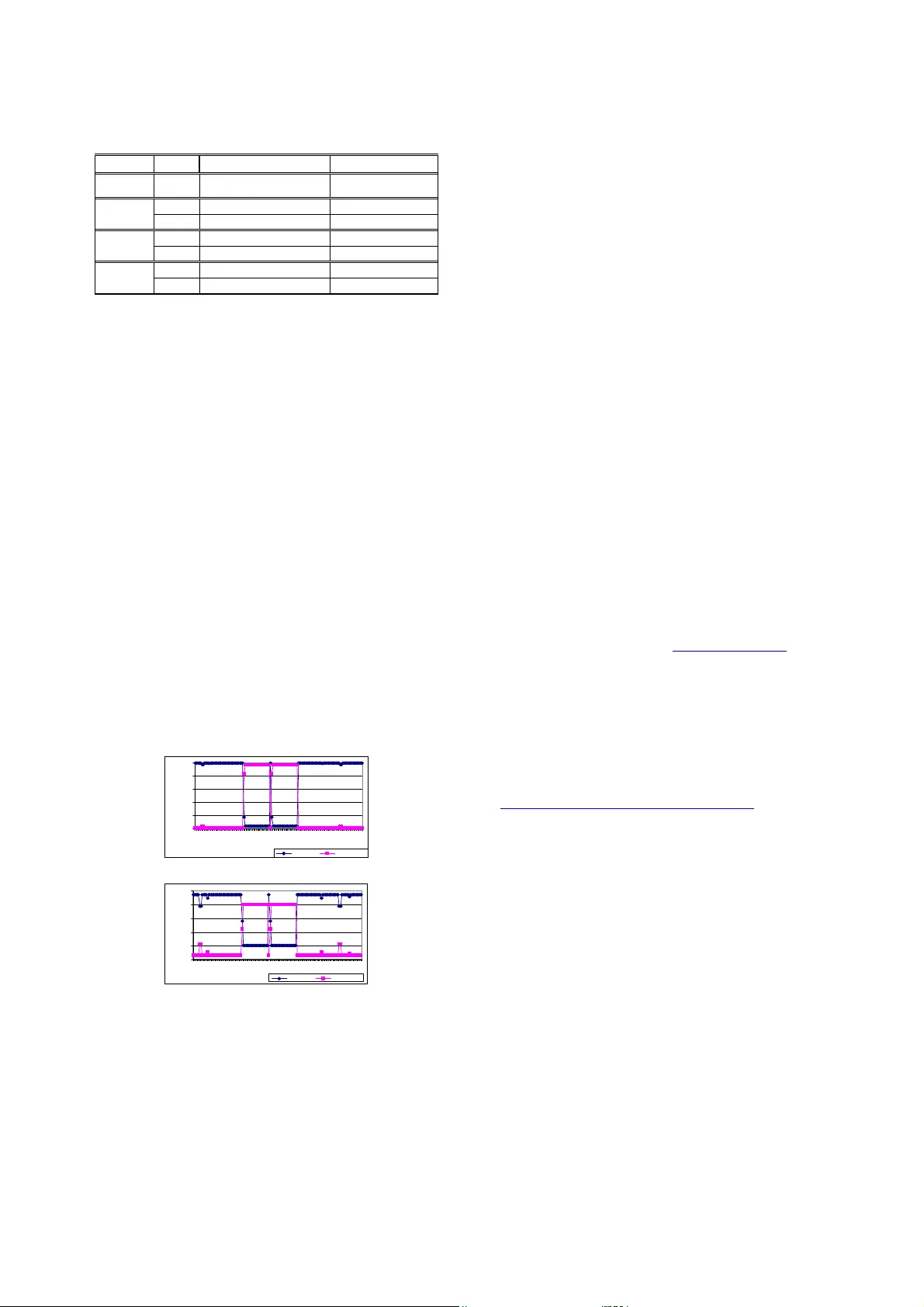
Abstract —In this paper, we imp lem ent an ano ma ly detect ion system using the Dem pster -Shafer m ethod . Using tw o st anda rd bench m ark problem s w e show that by co m bining mu ltiple signals it is possible to achieve better results than by usin g a single signal. We further show tha t by applying this ap proach to a r eal-world em ail dataset t he algorith m works fo r email w orm detection. Dem pster-Sha fer can be a prom ising m et hod for ano ma ly detection prob lems with multip le features ( data sourc es), and two or mo re classes. I. I NTRODUCTI ON Intrusion Detection Syst ems (IDSs) p lay a p ivotal ro le w ithin network security [1 ]. IDSs are one of many too ls used to detect attacks and intruders of computer sy stems. It is important to no te that the purpo se of IDSs is not to prevent the entry of int ruders to a system, but to notify the administ rator of any observed intruders. IDS techniques can be categorised a s eith er mi suse detectors or anomaly detectors. Misu se detection sys tems, such as Snort [2], rely on intrusion signatures to detect an attack. Such signatures are s tored in a database, whi c h relies on freq uent updates to r emain functional. System behaviours are matched against the sign atures within the da tabase. I f a successful match is formed, an alert is generated. An administ rator can use these aler ts t o investigat e the p otential problem, and generate ap prop riate res ponses. H owever, like many anti-virus scanners, mis use-detectors rel y on continual updates of the sign ature database. Hence the main drawback w ith this paradigm is that it will never d etect ‘day-zero’ intrusions to wh ich signatu res have not yet been created. Conversely, anomaly detection techniques generat e profiles of nor mal behaviour. Devia tions fro m the ‘normal profile’ result in the generation of alerts, whi ch ar e used by the system administrator for audit purp oses. T he major advantage of anomaly detectio n system s is that novel attacks can b e detected. Unfortunately, the pro files are not alw ays accurate, as user behaviour changes o ver tim e. This c an lead to the g ener ation of false positive alerts, w hen previously unseen user b ehaviour occurs for le gitim ate reasons. T he false po sitive rate can be suff iciently high that the anomaly detection system can b e flood ed by these alerts, forcing the administ rator to either ignore the alerts or disable t he system . Our work is part o f the research to reduce the num ber of false alerts prod uced by anomaly d etection system s. Q. Chen is with th e school of Computer Science & IT, Univers ity Of Nottingham, Nottin gham, NG8 1B B, UK. (phone: 0115-9 51-424 7; fax: 0115-9 51-425 4; e-mail: qxc@ cs.nott. ac.uk). U. Aickelin is with t he school of Comput er Sci ence & IT, University Of Nottingham, Notti ngham, NG8 1BB, UK. (e-mail: uxa@cs.nott.ac.uk ). A considerabl e number of ano maly detection system s have been developed . Examples i nclude [3] wh o employ ed statistical and grammatical m et rics to detect anomalies within system cal ls, and [4] w hich used an immun e-inspired system to detect ab normal processes. Anomal y detection is not r estricted to co mputer security. Other app lications such as threat assessment and m edical diagnosis rely on detecting deviations within dyn amic environments . One technique used for detection is Multisensor Da ta Fusion [5] . T his i s a form of signal proces sing, where data from multiple sources is used for analysis . The Dempster-Shafer t heory o f inference is a statistical method, considered as a generalised Bay es ian theory, whi ch can be used to combine multiple s treams of input data. We believe that the Dempster-S hafer method can be successfully app lied to anomaly detectio n through assigning ‘ belief values’ to inputs from v arious data sources. The remainder of this pap er is organised as fol low s. Section II disc usses the f undamentals of the Dempster-Shafer Theo ry and its advantages a nd d isadvantages. An anomaly detection appro ach using t he Dempster-Shafer theory is presented in III. We give some experi m ental results for two standard benchmark p roble m s in IV and V . These two datasets are the Wisconsin Bre ast Cancer Dataset and the Iris dataset of the UCI Machine Learning Re pository [6 ]. T he experiment results for the email worm dataset (collected b y our coll eague) are described in VI. VII co ncludes the paper . II. THE DEMPST ER - SHAF ER ( D - S ) THEORY The Dempster-Shafer (D-S ) theory is a m athematical theory o f evidence, introd uced in the 1960 's by Arthur Dempster [7] an d d eveloped in the 1 970's by Glenn Shafer [8]. T he D-S T heory is viewed as a mechanism for reasoning under ep istem ic (know ledge) uncertainty. T he p art of the D - S theory w hich is of direct relevance to our w ork is the Dempster’s rule of com bination . We present some e ssential mathem at ical terminologies in section A, before we introduce the Demp ster’s rule of combina tion in B . We introduce the advantages and d isadvantages of D-S in C. A. B asic mathem atical terminol ogy Frame o f d iscernment ( Θ Θ Θ Θ ) is a finite set mu tually exclusive propo sitions and hypotheses about some problem domain. Basic p robability a ssignment (b pa) is stated in [8] as : “If Θ is a frame of d iscernment, then a function m : [ ] 1 , 0 2 → Θ is called a basic prob ability assign ment wh enever 0 ) ( = φ m (1 ) and Anomaly Detection Using the Dempster -Shafer Method Qi Chen and Uwe Aickelin ∑ = Θ ⊂ A A m 1 ) ( . (2) The mass value of A (m ( A)) is also ca lled A’s basic proba bility num ber , and it is understood to be the measure of the belief that is commi tted exactly to A.” Belief function (Bel) is a b elief m easure of a pr oposition A, and it s um s the mass value of all the non-empty subsets of A. This subset is also called the focal element of the Bel . ∑ = ⊆ A B B m A Bel ) ( ) ( (3) Plausibility function (Pl) takes into acco unt all the el ement s related to A (either supported b y evidence or unknow n). ) ( 1 ) ( A Bel A Pl ¬ − = (4) For the subset A, Bel( A) and Pl (A) represent upper and lower belief bounds, a nd the int erval [Bel( A), P l(A)] represents the b elief range. T he relationships between Be l value, Pl value and uncertainty are describ ed in Figure 1. Fig. 1. The uncertainty int erval for a hypothesis [9] B. The Dempster’s Ru le of Combina tion ∑ − ∑ = = ∩ = ∩ φ C B A C B C m B m C m B m A m ) ( ) ( 1 ) ( ) ( ) ( 2 1 2 1 12 (5) We can use Dempster’s rule of co mbination to combine the mas s values of all features from each indi vidual sensor to achieve the overall summ a ry mass values for each sensor. These summ ary values fro m all sensors ar e combined to give the sum mary mass valu es for the system . Initially, the bpa s are used to assign the mass values t o appro priate hypothesis. Then the resulting mass values are used to calc ulate t he belief for the ap propr iate hy po thesis. Finally all beliefs are combined with D empster’s rule of combination to gain the over view belief for t he approp riate hypothesis, as show n in Equatio n (5). C. Advantages and Disa dvantag es of D-S The main advantage of D-S is that no a priori know l edge is r equired, making i t potentially suitable for anom al y detection of previously unseen information. Anoth er advantage is that a value for i gnorance can b e expressed, giving information on the uncertainty of a situation. Bayesian inference requires a p riori knowl e dge and does not allow allocating p robabi lity to ignorance. It can only express the proba bility of an event being either abnormal or normal. It is our opinion that a Bayesian app roach is not al w a ys suitable for anomaly detection because pre -existing knowledge may not alw ays be pro vided. In particular, if the aim is to detect previously unseen attacks, then a system which relies on existing k nowledge cannot be used. There are two m aj or problems as sociated with D-S: the computation complexity and conflicting belie fs managem ent. The computational complexity increases exponentially w it h the number of frames of discernment ( Θ ). If there are n elements in Θ , there will be up to 1 2 − n focal element s for the mass function. T he combination of two mass function s needs the computation of up to n 2 intersections. To overcome this, various algorithms, such as [10 ] and [11 ], have been suggested to reduce t he focal element number in the involved mass functions. For anomaly detection, the resulting computation co mplexi ty is lo w , as the frame o f discernm ent consists of only tw o e lem e nts ( normal and abno rmal). T here are up to three fo cal elements of belief functions: {normal}, {abnormal}, and {normal o r abnormal} (i.e. the uncertainty), resulting in low com putatio n complexity The Dempster’s r ule of co mbination redistrib utes the mass values o f empty p ropositions to non-empty p ropositions, also known as normalization step, due t o the d efinition of the mass f unction. This som et imes leads to erroneous results, whi ch causes the conflicting m a nagemen t problem. In order to solve this problem, som e alternative combination rules have been pr oposed, as in [12 ] and [13], but none have yet been accepted as a standard method. In ord er to illustrate this probl em, co nsider the following example: a car w i ndow has been bro ken, and the culprit needs to be id entified. T here are three suspicious peo ple (Jo n, Mary, and Mike) and two witness es (Witness1 and W itness2). W itness1 a ssigns “Jon broke it” w ith a mass value of 0.9 , and “Mary br oke it” with a m a ss value o f 0 .1; w itness2 assigns “Mike broke it” with a mass value of 0 .9, and “Mary b roke i t” with a mass value of 0.1. Both wi tnesses assign a very small mass value to “Mary broke it”. Applying the D empster’s rule o f combination for “Mary broke the window”, returns a value of 1, w hich is not accurate. Thi s is bec ause the mass val ue can be affected by taking into account conflicting opinions of multiple sources. For our anomaly detection applicatio n, each bpa w ill assign a non-zero mass value to {normal or ab normal} as the erro r rate; therefore we will not face any belief conf l ict problems. In sum mary, the D-S method is a combinat ion of a theory of evidence a nd pro bable r easoning, to derive a belief that an event has occurred. Individual beliefs are updated and combined to give a b elief of an event oc curring in the system as a whole. T hough a hotly deb ated point, D-S has advantages o ver B ayesian tec hniques w hen applied to anomaly de tection as described above. For o ur application, each b pa will assign a non-zero mass value to {normal or abnormal}, this avoids any belief conflict problems. III. THE AP PL I C ATI ON OF D - S I N ANOMA LY DETECT ION We implem ented a D-S sys tem and ap plied it to t w o standard b enchm ark prob lems of t he UCI datasets [6], the Wisconsin Breast C ancer Dat aset ( WBCD ) and the Iris Dataset, and one email dataset made by our colle ague. Two standard benchm ark dataset are chosen to co mpare our appro ach with the performance of o ther algorithms, and to investigate wh et her i t i s p ossible to achieve good results b y combining vario us features using D-S. The em ail d ataset is chosen, because it is in our interested applicatio n area. The anomaly d etection system uses a tra ining process to 0 1 Uncertainty Pl(A) Bel(A) Bel(⌐A) derive thresholds from the training data, and detects an event as normal or abnormal (as shown in figure 2). The bpa functions ar e built based on these thr esholds f or the purpose of assigning mass values. The anomaly detection appro ach is demonstrated in figu re 3. T he dat a from various sources are processed and sent to co rrespo nding bpa assignm ent functions. The mass values for each hypothesis are generat ed and s e nt to D-S combination component. This component uses the Dempster’s rule of combination t o combine all mass values; and g enerate the overall mass valu es for each hypothesis. T he data can be de tected as normal or abnormal based on the overall mass valu es for each hypothesis. Fig. 2. Data flow of the A n omaly Detection Syste m All exper iment s for the three chosen datasets w ere executed on an I ntel P entium 4 CPU, 1.5G Hz, 25 6MB RAM, Wi ndows 2 000 p latform computer. T he system was coded using Java 2 platform, Standard Edition (J2 SE) 1.4.0. The execution times (average running time of 10 r uns) for the three datasets a re: 30 seconds for the W BCD, 25 seco nds for the Iris datas et, and 12 second s for the email dataset. Fig. 3. Anomaly Detection Approach IV. EXPERI MENTS WI TH THE W B CD A. The Wisconsin breast ca ncer data set (WBCD) The WB CD is a standard benchmark d ataset of the UCI Machine Learning Repository [6]. This dataset is chosen for two obj ectives. O ne is to com p are our ap proach w ith the performance of o ther algorithms. T he o ther is to investigate w hether it is p ossible to achi eve good results by combining mu ltiple features using D-S, without excessive manual intervention or domain know l edge based p arameter tuning . The WBCD contains 699 data items: 241 malignan t items (abnormal data) , and 45 8 benign items ( normal d ata). T his dataset has nine features; all features ar e normalised integers in the ra nge b etw e en 1 and 10. A, B, C, D, E, F, G, H and I are u sed to represent the biological f e atures of A: Clum p Thickness, B: U niformit y of Cell Size, C: Uniformit y of Cell Shape, D: Marginal Adhesion, E: Single Epithelial Cell Size , F: Bare Nuclei, G : Bland Chromatin , H: Normal Nucleoli, and I: Mitoses, respectively. T here are 16 i nstances; each contains a single missing (i.e. un available) attribute value. Our D-S b ased anomal y det ection s y stem has the a bility to cope wi th this problem by omitting, i.e. not combining, the missing values of t he co rresponding data items. T his is an advantage of D-S o ver other app roaches, such as [14 ] [15], whi ch have to exclude the 16 items with m issing values. For the WBCD, the frame o f discernment of the system is {normal, a bnormal}. The bpa function and the t hreshold settings are illustrated in the next section. B. The classification a pproa ch We use ten fold cross validation in our exp erimen t . The dataset is d ivided i nto t en subsets of approximately equal size ( one subset size is e ither 69 or 7 0). Each time we use the data of one subset as test d ata, and the d ata o f t he other nine subsets as training data. T he training data is used to o btain the modif ied m edian threshold to build the bpa functions. The d ataset size i s 699, so the training d ata size is e ither 6 30 or 629. T he p ropor tional distrib ution of the WBCD is 65.5% :34.5% (normal: abnormal). We or der the training data feature values from small to large based on each feature. I f the trai ning data size is 630, t he 413 th small value o f one feature is chosen as the modified median threshold. If the training data size i s 62 9, the 412 th small value o f one feature is cho sen as the modified median threshold. W e use a general assum p tion that the lower value items tend t o be normal data. Then the bp a function for each feature is : ) ( 1 ) ( ) 1 ( 1 normal m abnormal m e m(normal) threshold) ( value − = + = − − (6). Figure 4 shows a graphical illustration of the shapes of functions using a sam p le threshold of 5. Note that for the probl ems we study , all data items ar e integers and hence the functions consist of discrete values only. 0 0.2 0.4 0.6 0.8 1 0 1 2 3 4 5 6 7 8 9 10 Fig. 4 . Part of the bpa fun ction for the WBCD, the x-axis shows feature values, y-axis show s mass values All thresholds for n ine featu res are found, and t he bpa functions are built for each feature. For each data item , the bpa fun c tions are used t o assign the mass values for each feature based o n that feature value. For that data item, all mass values are combined to obtain the over all mass values of the hypothesis normal and of the hypothesis abnormal. If the mass value of the ‘abnormal’ hypothesis is bigger than the mass valu e of the ‘normal’ hy po thesis, then it is classifi ed as abnormal; otherwise it is classified as normal. C. E xperimental results for the WBCD To j udge the q uality of results, w e compare the data from various sources/features data 1 data 2 data n bpa assignment bpa assignment bpa assignment …… …… m 1 (H) m 2 (H) m n (H) D-S combination m 12…n (H), m 12…n (¬H) …… Data is normal or a bnormal training dat a data training thr eshold(s) Anomaly Detection Event is no rmal o r abnormal classification accuracies, based on the followin g definition: classification accuracy = items of number Total items classified correctly of Number . 75 80 85 90 95 100 A B C D E F G H I A + D +I B +C +F N ine f e atu re s Used feature(s) C la s s if ic at io n A c c u ra c y (% ) Fig. 5. Classification accuraci es wit h various features for the WBCD Figure 5 s hows that feature A (classification rate 86.0 %), D (85.7%) and I (79.3%) give the poo rest perfor mance wh en using o nly o ne feature at a time. The result when combing mu ltiple features ( A, D and I) together (9 0.0%) is better than using either A, D or I a lone. Features B (92.7 %), C ( 92.1 %), and F (91.3%) are the best three features when using only one feature at a time. Similarly the result of combining these three (95.7%) is better than using either of them alone. T he result o f using all nine features (97 .6%) is bet ter than any other combination of features. Our first hy pothesis that co mbini ng features using D-S improves ac curacy is proven corre ct for the W BCD Moreover, o ur second assumption is a lso pr oven co rrect, i.e. a few b adly chosen features do not negatively influence the results, as long as m o st ch osen features ar e suitable. T hese two characteris tics make D-S very amenable for solving real- w orld I DS problems. D. Comparison with other method s To appr eciate the high quality of our res ults, we pro vide a comparison w i th o ther p ublished results. [14] used a generalized rank nearest neighbour rule and achieved a classification rate of 96.17%; also [15] used a fuzzy classification method, with a b est re sult o f a classification rate equal to 96.7%. Both methods i gnore the 16 W BCD data items w it h missi ng feature values. Our classification rate compares favourably w ith these being 97.6% (including all data with mi ss ing feature values). T he ability to deal with missi ng values is important for network security pr oblems. Our method has the advantage of having such ability. V. EXPERI M ENTS W ITH TH E IR IS PL ANT DATA SET A. The Iris pla nt dataset The Iris plant d ataset is another standard b enchm a rk problem o f the UCI data sets [6]. T his dataset is c hosen because it has fe w e r features and more classes than the WBCD. T his w i ll confirm whether D-S ca n work on problems with fewer features and m ore classes. This dataset has 1 50 instances with the follow ing four num er ic features: sepal length in cm; sepal width in cm; petal length i n c m; and petal width in cm. T he dataset also contains o ne p redictab le feature, namel y the class lab el. These 150 in stances are of three classes ( plant ty p e), Iris Setosa , Iris Versicolour, and I ris Virginica , with each class containing 50 instances. B. The classification a pproa ch The I ris instances distribution overlapping information, based on individual feature, is used to ro ughly classify the Iris data (as shown in Figure 6 ). A num ber of items ar e not classified into a single class, such as either Setosa o r Versicolo ur. For such data items, we use the difference between a da ta item value and the mean value of the sel ected suitable feature to provide classification into individual single classes. This classification approach is achieved in three steps, as descr ibed bel ow. In the first s tep , the sy stem use bpa A to assign m ass values to all the four features of one data item based on the boundary inform ation. For this data item, the sys tem combines the mass values using the Dempster’s rule of combination, and then generates the overall mass values and belief values for all p ossible. There are seven p ossible hypotheses for the Iris dataset: {Setosa}; {V ersicolour}; {Virginica}; {Seto sa, Versico lour}; {Setosa, Virginica}; {Versicolo ur, Virginica}; and {Setosa, Versicolour, Virginica}. The data item is classified to t he hypothesi s with the highest b elief value. If with the results of first step, the data item is not classified to a single cla ss, such as {Setosa, Versicolo ur}, then the sys tem uses the second step to classify it to a single class. In th e second step, initially th e mo st suitable feature is selected. Following this, the sys tem uses the bpa B to assign mass values based on t he distance to the mean values of the three cl asses of that feature. In the third step, the system combines the mass values of step one and step tw o . T he o verall mass values and the b elief values are calculated. T he items ar e classified to the hypothesis with the highest belief values. We use ten fold cross validation in our exp erimen t . The dataset is divided into ten subsets o f equal size , with nine out of ten subsets comprising tr aining d ata, with the remaining subset used as test d ata. The training data is used to obtain the thresholds to build the bpa assignment functions. The follo w ing parts of sectio n V ar e organised as b elow. Section B.1 detai ls how to use b pa A to assign mass values based on the b oundary information. I n section B.3, we demonstrate the use of bpa B a ssign ing mass values based on the d ifferences between a feature value and the mean feature values of three classes. Finally the selection o f suitable features is described in section B.2. B.1 bp a (basic p robability assig nment) funct ion A Firstly, we need to find the maximum and minimu m v al ues for each class based on one feature of the trai ning data. T hen we calculate the o verlapping part for the three class es, to obtain the boundary informat ion for each class, based on this feature of the training data, as show n in Figure 6. Fo r Figure 6 and 7, each o f the vertical lines is the value range for one class of one f eature; the horizontal lines are used for comparison to calculate the overl ap. class 1 , class 2 , class 3 ∈ {{Setosa}, {Ver s icolour}, {Viginica}}. Fig. 6. Example: for o n e feature, how to calculate the th ree cl ass overlap We use the example o f Figure 6 to illustrate how to calculate t he overlap. If the value is less than min(class 2 ), and greater th an or equal to min(class 1 ), the data item must belong to class 1 . T his is b ecause all the values of the data items belonging to class 2 shou ld not b e less than min(class 2 ). Sim ilarl y, the values of the data items belonging to class 3 should be not less t han min(class 3 ). In t his cas e, the min(class 3 ) i s b igger than min (class 2 ), so the values of the data items belong to cl ass 2 or c lass 3 should not be l ess than min(class 2 ). For the same reason, d ata items wit h values greater than max(class 2 ), belo ng to class 3 . D ata i tem s with values between min(class 2 ) and min(class 3 ) belong to class 1 or class 2. Data items with value betw een mi n(class 3 ) and max(class 1 ) belong t o class 1 or cl ass 2 or class 3. For data items containing val ue b etween max (class 1 ) and max(class 2 ) belong to class 2 or class 3. Fig. 7. Example of minimum, maximum value settings for F ig. 6. In Figure 7, we set example maximu m and minim um values, to illustrate the assignm ent of the mass values based on the boundary information. For one feature, if the feature value is less than min(class 1 )=1, then that dat a item is classified as class 1 . W e assign m(class 1 )=0.9, and 0.1 ) m( = Θ based on that feature alone. A s nothing is hundred percent accurate, we think t he trustiness of this measu rement is 0.9, and set the uncertainty ( ) m( Θ ) as 0.1. For each featur e, we have the bpa function A: 0.1; ) m( 0.9, m(class1) ), 5 . 2 , ( = Θ = −∞ ∈ value if 0.1; ) m( 0.9, class2) (class1 m ), 3 , 5 . 2 [ = Θ = ∪ ∈ value if 1; ) m( ], 4 , 3 [ = Θ ∈ value if 0.1; ) m( 0.9, class3) (class2 m ], 5 . 4 , 4 ( = Θ = ∪ ∈ value if 0.1 ) m( 0.9, m(class3) ), , 5 . 4 ( = Θ = +∞ ∈ value if . In the first step, w e app ly bpa function A to each feature of one data item, and use the Dempster’s rule o f combination to c ombine the mass values of the four fe atures. T his generates the overall mass values for that data item. The overall classification is d ecided b ased on the o verall mass values. If the d ata item is not classified to a single cl ass, then we w il l use the second step. B.2 Fea ture selection Suitable features m ust be sele cted in o rder to separate tw o or three cla sses using the d ifference between the data item value and the m ean value o f t he three classes. A feature is required with t he followin g characteristics: the d ata f eature values of o ne single class are close together; and the values of t w o c lasses view ed as a group ar e far a part. This is achieved by cal culating the standard d eviation for the two classes, and the standar d deviation for the union of these two classes. T his is defined as the Feature Se lection Value ( F SV ), shown in Eq uation 7. The fe ature wi th the smallest FSV is chosen as the suitable feature. The Feature Selection V alue (FSV) for n (a natura l number) classes is: ) ( ) ( ) ( ) ( 2 1 2 1 n n class class class sd class sd class sd class sd FSV ∪ ⋅ ⋅ ⋅ ∪ ∪ × ⋅ ⋅ ⋅ × × = (7 ) For e xam p le, to separate the class Setosa and the class Versicolour, we select the featu r e with the smallest FSV= r) Versicolou sd(Setosa lour) sd(Versico Setosa) ( ∪ × sd . B.3 bpa (basic probabi lity assignment) function B In the second step, a suitable feature is selected and the bpa function B is used to assign mass values. W e build bpa function B based on the inform ation of the absolute distances (defined as difference in Equation 8) between the data item value of the chosen feature and the mean feature value o f each class. Here, we wan t to classify the data item as the class wi t h the sm allest difference. class one of mean value difference − = (8). The inform atio n of bpa B is viewed as less important than the informat ion of bpa A . The mass value of one affected hypothes is is set as 0.8, the uncertainty as 0.2. We have the follow ing bpa function B: if Setosa has the smallest difference, then s et m ( Setosa )=0 .8, 0.2 ) m( = Θ ; if Versicolour has the sm allest difference, then s et m ( Versicolour )=0.8 , 0.2 ) m( = Θ ; if Virginica has the smal l est difference, then set m ( Virginica )= 0.8, 0.2 ) m( = Θ . C. Exp erimental results with the Iris Plant data set The classification accuracy with the Iris p lant dataset i s 95.47% ± 0.48% (of ten runs). Tab le 1 shows three out o f ten of the experimental results ( chosen randomly for illustrative p urpose). These r esults are based on the whole application ap proach w i th d etailed er ror information and results. The table label meanings are explained below. • ‘Id’: one item’s identifi cat ion number. 1-50: ids of Setosa, 51-100: ids of Versicolour, 101-150: ids of Virginica. • ‘Corre ct(1st)’: the number of correctly classified items using t he 1 st step wit h the boundary inf or mati on. min(class 1 ) class 3 class 1 class 2 or class 3 class 1 or class 2 class 1 or class 2 or class 3 min(class 2 ) min(class 3 ) max(class 2 ) max(class 1 ) max(class 3 ) class 1 ≠ class 2 ≠clas s 3 min class1 = 1 min class2 =2.5 min class3 =3 max class2 =4.5 max class1 =4 max class3 =5.5 class 1 ≠ class 2 ≠clas s 3 • ‘Error s(1st)’: the number of er rors caused by the first step w hich only use the boundary i nformation. • ‘In two(1st)’: the num ber of date items, wh ose results are not in a single cl ass after the first step. • ‘Error s(2nd)’: the erro rs caused by the second step which use the “ difference” inf ormation T ABLE 1 THE I RIS P LAN EXPERIMENTS USI NG THE WHOLE APPROACH 1 st Run of the experiments—classification accuracy=96.666 7 I d Correct(1 st ) Errors(1 st ) I n two(1 st ) Erro rs(2 nd ) 1-50 50 0 0 0 51-100 35 2 ( Id= 71, 86 ) 13 Id=78 101-15 0 42 2( Id=107,12 0 ) 6 0 2 nd Run of th e expe riments—classification accuracy=95.3 333% I d Correct(1 st ) Errors(1 st ) In two (1 st ) Erro rs(2 nd ) 1-50 50 0 0 0 51-100 33 4( Id=51,7 1,84, 86 ) 13 Id=78 101-15 0 42 2( Id=107,12 0 ) 6 0 3 rd Run of th e expe riments—classificati on accuracy=94.6 667% I d Correct(1 st ) Errors(1 st ) In two (1 st ) Errors(2 nd ) 1-50 50 0 0 0 51-100 34 5( Id=51,5 7,71,84 ,86 ) 11 Id=78 101-15 0 43 2( Id=107, 120 ) 5 0 The data items 71 , 86, 107 and 12 0 are w r ongly classif i ed in all these three runs, due to the first step of the classification ap proach. The 78 is wrongly class i fied in all three runs, due to the second step of the classifi cation. In Table 2, the parameters used in the 2 nd run of the experiment s for data 86 are show n. W e use this exam ple to show how some mi s takes may occur. 86: F1-6 (classified as class 23 ); F2-3.4( class 13 ); F3-4.5(class 23 ); and F4 -1.6 ( class 23 ). It is classified as class 3 using the 1 st step, which is wrong . F1, F3, and F4 express belief of class 23 , and F2 expresses belief of cl ass 13 . The combination r esult is class 3 . One plausible reason is that the training data does not include all the information of the tes t data; perhaps the param et ers are not totally accurate. For the same reason, t he data item 7 8 is w r ongly classified due to the 2 nd step. T his can b e improved by combining 1 st and 2 nd steps together. If w e use 1 st and 2 nd step together for all the d at a, the expected resu lts can be improved. W e can also use a finer grained model to extract these individual features of the Iris d ata, which can also lead to better perfor man ce. TABLE 2 THE PARAMETERS OF THE TRAI NING SET FOR THE DATA ITEM 86 Class 1 Class 2 Class 3 max 5.8 6.9 7.9 Feature1 (F1) min 4.3 4.9 4.9 max 4.4 3.3 3.8 Feature2 (F2) min 2.3 2.0 2.2 max 1.9 5.1 6.7 Feature3 (F3) min 1.0 3.3 4.5 max 0.6 1.7 2.5 Feature4 (F4) min 0.1 1 1.4 D. Co mparison with other metho ds The classification accuracy o f our method applied to the Iris data i s 95.4 7% ± 0.48% over 10 runs. It is sim ilar as published re sults of other established methods ( w hose results are be tw een 94.6 7% and 9 7.33%) [ 16]. T his d em onstrates the ability of D-S to successfully cl assify item s within datasets comprising few features and mu ltip le classes. VI. EXPERI MENTS WI TH EMAI L DA TASETS We have confirmed th e potential of D-S to produce rob ust, high quality results. T hen w e t urn our attention to the probl em of w orm detection. Due to t he lack of datasets, we have derived our o w n data suitable for t he detect ion of email worm s. Worm detection for ms a large subset of compu t er security and provides us with a m anaged prob lem to solve. A. Th e email dataset Email dat aset was created by combinin g a week's w orth of emails (90 emails) from a user's sent box w ith outgoing emails (42 emails) sent by a computer infected with the netsky-d worm. T he aim o f this experiment is to correctly detect the 42 worm infect ed emails. With expert experience, we deci de to use these attributes of each individual email: its sender is spoofed o r not; whether i t contains dangerous attachm ents, wh e ther it contains non-dangerous attachm ents, the tim e interval since last em ail w as sent. This information is listed in Table 3. Spoofed sender can be defi ned as a sender with a fake email address; pif: program information file, i.e. a d angerous file type; doc: word file (Considered as non-dangerous here). T ABLE 3 SUMMARY OF THE EMAIL DATAS ET Message Sp oofed Send er number & type of atta chments 39-59 (worm) Yes 1 pif 61-81 (worm) Yes 1 pif 12, 101 No 1 doc Others No 0 B. The worm detection process The four features used here are : signal1 – t he time interval from last message sent, sign al2 – the sender (spoo fed-1, normal- 0), s ignal3 – wheth er there are any dangerous attachm ent files (0 – no, 1 – yes), signal4 – wh ether there are some non-dangerous attachment files (0 - no, 1 - yes). Signal1 has a big range and varies from 0 t o 946 65, its bpa function is presented in Figu re 8, the bpa fu nctions used by the other three features are described in Ta ble5. 0.2 0.3 0.4 0.5 0.6 0.7 0 10 20 30 40 50 m a s s v a lu e Fig. 8. bpa for signal1, the x-axis shows seconds sin ce last email With experience, the signals can be r anked in order of importance (high to low): signal2, sign al3, si gnal1 and signal4. T hreshold settings were decided following this order (shown in Table 4). Fro m this information, mass value settings w ere deri ved, as show n in T able 5. TABL E 4 THRESHOLD SETTI NGS FOR EMAIL DATA SET Featur es thresho ld Min m(normal ) Max m(normal) Sign al 1 3 0 0.3 0.7 Sign al 2 1 0.1 0.9 Sign al 3 1 0.2 0.8 Sign al 4 1 0.4 0.6 TABL E 5 MASS VAL UE SETTINGS FOR EMAIL DATA SET ( M ( Θ )=0.01) value m(normal) m (a bnormal) Signa l 1 =value 3 . 0 ) 1 ( 4 . 0 1 30 + + − − ) ( value e 1- m ( normal )- ) ( Θ m =0 0.9 0.09 Signa l 2 =1 0.1 0.89 =0 0.8 0.19 Signa l 3 =1 0.2 0.79 =0 0.6 0.39 Signa l 4 =1 0.4 0.59 We a ssign the mass values for ea ch individual feature of one em ai l using the settings in Table 5. T hese mass values for the same em ai l are combined using t he co mbin a tion rule based on each individual hy pothesis. The overall mass valu es of each hy pothesis are generated. T hat email is classifi ed as the hy pothesis w ith the higher overall mass value. C. Experimental Results with email dataset When using four signals, all 42 worm infected emails were detected co rrectly, as show n in Figure 9. As it is not alway s easy to determine a spoofed sender, we re-run the experiment s r emovin g t his signal (Figure 10). Messages 39 and 61 were undetected wh en using the three r em aining features (i.e. signal1, signal3, and signal4). T he w r ongly classified m essages are those mes sages sent directly aft er legitim ate traffic. Hence, the time intervals sin ce last messag e sent of the two messag es appear normal, w i th the only ab norm al features being the executable attachment. Because all the three features have simi lar weight s, and tw o of them indicate that the emails are normal, they are wrongly classified as normal. T his can be corrected by w eight ing these features with greater d ifferent m ass values, or adding in more effective fe atures. A more effective feature can be the num be r of w o rds contained in an e mail. W e wil l look into these issues in fut ure experiments . 0 0.2 0.4 0.6 0.8 1 1 14 27 40 53 66 79 92 105 118 13 1 email Id m va l ue Nor mal Abno rmal Fig. 9. Results of email da ta usin g all four features 0 0.2 0.4 0.6 0.8 1 1 11 21 31 41 51 61 71 81 91 101 111 121 131 email _ ID m V al ue Nor m al Abnormal Fig. 10. Results of em ail da ta usin g signal1, signa l3, signal4 VII. C ONCLUS I ONS The experimental results for the WBCD (with nine features and two classes) show that we successf ully classify a standard dataset by co mbin g multiple feat ures usin g the D-S method. The results for the Iris dataset (with four f eatures, three classes) show that we ca n also use D-S for problems w i th more than two classes, w ith few er features. Our sy stem successfu lly detects email worms through experimen ts with a realistic email dat aset. These res ults indicate that D-S method works successfully for anomaly detection by combing the beliefs from mu ltiple sources. Based on these results, we can co nclude that D-S can b e a promising method for network security prob lems w ith mu ltiple features (from various data sources) and two or more classes. Of course, like other classification algorithm s, the initial feature selection influences overall performance. Howev er, due to the inherent ro bustness of D-S, as long as there the majority features are suitable, o ur system still works, even if some features ar e poor . Furtherm o re, our approach works in situations wh e re some feature values are miss ing, which is likely to o ccur in r eal world netw ork security scenarios. Our continuing aim is to find out how D -S b ased algorithms can be used m o re effectively for the purpose of anomaly detection withi n the domain of netw ork security . VIII. ACK NOWL EDGEMENTS The authors would like to thank Julie Gr eensm ith for useful co m men ts and J am ie T wy cr oss for collecting the email dataset. R EFERENCES [1] E. Schultz, “Demystify ing I ntru sion De tecti on: Sorting through the Confusion” , Hyperbole and Misconceptions . Networ k Securit y, 2002, pp. 12-17. [2] Snort Intrusion Detection Systems. http://www.snort.org [3] C. Kruegel, D. Mutz, F. Valeur, an d G. Vigna, “On the Detection of Abnormal System Call Ar gum ents”, Proceedings of ESORICS 2003, LNCS, Springer-Ve rlag Gjovik, Norw ay, 2 003, pp. 32 6-343. [4] A. Somayaji and S . F orrest., “Automated R esponse Using Sy stem- Call Delays”, Proceedings of t he 9th USENIX Security Symposium, The USENI X Associati on, Berkeley , CA, 2000 . [5] Hall, D. L., and H. A. Sonya, Mc Mullen, Mat hematical Techniques i n Multis ensor Data Fusion, 2 nd Edition, Artech House, Boston-London, 200 4. [6] C. Blak e and C . J. Merz, UCI machine learning repository, http ://www .ic s.uci.edu/ ~mlearn/MLRepository .html [7] A.P. Dempster, “Upper and lo wer probabiliti es induced by a multivalued map ping”, Ann. Mat h. Statis t., 196 7, pp. 325 -339. [8] Shafer, G., A M ath ematical Theory of Evidence, Princeton Uni versity Press, Princeton an d London, 1976 . [9] Law r ence, K . A, S ensor a nd Data F usion: A T ool for I nformation Assessme n t an d Decision Mak ing, SPIE, Washington, 20 04. [10 ] B. Tessem, “Approximations for efficient computation i n the theory of evidence”, Artificial Intellig ence, 199 3, pp . 315-3 29. [11 ] F. Voorbraak, “A comp utati onally efficien t app roximation of Dempster-Shafer theo ry”, Internat. J. Man-Ma chine Stud. 1989, pp. 525 -536. [12 ] R.R. Ya ger, “On the Dempster–Shafer framew ork and new combina tion rules”, Information Sciences, 1 987, pp . 93 –138. [13 ] C.K. Mu rphy, “Combini ng belief functi ons when evidence conflict s”, Decision Sup port System, 2000, pp. 1– 9. [14 ] S.C., Bagui, S. Bagui, K. Pal, and N. R. Pa l, Breast canc er detection using rank nearest neighb or classificati on rules, Pattern R ecognition, 200 3, pp. 25-34 . [15 ] D. Nauk , and R . Kruse, A neuro-fuzzy method t o learn fuzzy classifica tion rules from data, Fuzzy sets and Systems, 199 7, pp. 27 7- 288 . [16 ] Chen, S., a nd Fan g. Y, “A new appr oach fo r ha ndling the iris da ta classifica tion p roblem, International J ournal of Applied Science and Engineering, 2 005 3 , 1:37-49 .