Tropical Implicitization and Mixed Fiber Polytopes

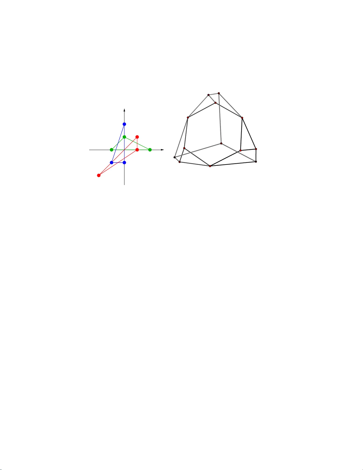
TR OPICAL IMPLICITIZA TION AND MIXED FIBER POL YTOPES BERND STURMFELS ∗ AND JOSEPHINE YU † Abstract. The softw are T rIm offers implement ations of tropical impli ci tization and tropical elimination, as dev elop ed by T evelev and the authors. Giv en a p olynomial map with generic coefficient s, T rIm co mputes the tropical v ariet y of the image. When the image is a hypersurface, the output is the Newton polytop e of the defining p olynomial. T rIm can th us b e used to compute mixed fib er p olytop es, including secondary polytop es. Key words. Elimination theory , fiber polytope, implicitization, mixed v olume, Newton p olytope, tropical algebraic geometry , secondary p olytop e. AMS(MOS) sub ject cla ssifications. 14Q10, 52B20, 52B55, 65D18 1. In tro duction. Implicitization is the problem of transforming a given parametric representation of an alge br aic v a riety into its implicit representation as the ze ro set of po lynomials. Most algor ithms for elimi- nation and implicitization are based o n m ultiv ar iate res ulta nt s or Gr¨ obner bases, but current implement ations of these metho ds are o ften too slow. When the v a riety is a h yp ersur face, the co efficients of the implicit equation can also be computed by wa y of numerical linear a lgebra [3, 7], provided the Newton p oly to pe of that implicit equatio n can be predicted a pr iori. The pr o blem of predicting the Newto n p olyto p e w as r e cently solv ed independently by three sets of authors, namely , by E miris, Kona xis and Palios [8], Ester ov and Khov ansk ii [13], a nd in our joint pap ers with T ev elev [18, 19]. A ma in conclusion of these papers can be summarized a s follows: The Newton p olytop e of the implicit e quation is a mixe d fib er p olytop e . The first ob jective of the pres ent article is to explain this conclusion and to pr esent the soft ware pac k a ge TrIm for computing suc h mixed fiber po lytop es. The name of our progra m stands for T r opic al Implicitization , and it underlines our view that the prediction of Newton po lytop es is best understo o d within the la r ger con text of tro pic a l algebraic geometry . The general theo ry o f tr o pical e limina tion developed in [18] unifies earlier results on discr iminants [4] and on ge ne r ic p olyno mial maps whose images can hav e any co dimension [19]. The second ob jectiv e of this a r ticle is to ex pla in the main res ults o f tropica l elimination theory a nd their implemen tation in TrIm . Numerous hands-on examples will illus tr ate the use of the s o ft ware. A t v arious places we give pre c ise po int ers to [8] and [13], s o as to highlight similarities and differences amo ng the different approa ches to the sub j ect. Our presentation is o rganized as follows. In Section 2 we start out with a quick g uide to TrIm b y showing so me simple computations. In Section ∗ Unive rsity of Californi a, Berkeley , CA 94720, bernd@math.b erkeley . edu † Massac huset ts Institute of T echnology , Cambridge, MA 02139, jyu@math.mit.edu 1 3 we explain mixed fibe r polytop es . That expo sition is self-co ntained and may be of indep endent interest to combinatorialists. In Section 4 we discuss the co mputation of mixed fib er p o lytop es in the co n text o f elimination theory , a nd in Section 5 we show how the tr opical implicitizatio n problem is solved in TrI m . Theorem 5.1 expresses the Newton p olytop e of the implicit equation a s a mixed fib e r p olytop e. In Section 6 we present results in tropical geometry on which the de velopment o f Tr Im is based, and we explain v arious details concerning o ur algo r ithms and their implementation. 2. Ho w to use TrIm . The first step is to do wnload TrIm from the following website which contains informatio n for installation in Linux : http:/ /math .mit.edu/ ~ jyu/Tr Im TrIm is a collection o f C++ pro grams which are glued tog e ther and in- tegrated with the ex ter nal s o ft ware polymake [9] using perl scripts. The language pe rl was c hosen fo r e a se of interfacing be t ween v a r ious progr ams. The fundamental pr oblem in tro pical implicitization is to compute the Newton p olytop e of a hyper surface which is parametr ized by Laur ent poly - nomials with sufficient ly ge neric co efficients. As an example we consider the following three La urent p o ly nomials in tw o unknowns x a nd y with sufficiently gener ic coe fficie nts α 1 , α 2 , α 3 , β 1 , β 2 , β 3 , γ 1 , γ 2 , γ 3 : u = α 1 · 1 x 2 y 2 + α 2 · x + α 3 · xy v = β 1 · x 2 + β 2 · y + β 3 · 1 x w = γ 1 · y 2 + γ 2 · 1 xy + γ 3 · 1 y . W e seek the unique (up to scaling) irre ducible p olynomial F ( u, v , w ) which v anishes on the image of the cor resp onding morphism ( C ∗ ) 2 → C 3 . Using our softw are TrIm , the Newton polytop e of the p olyno mial F ( u, v , w ) can be computed as follows. W e first create a file input with the con tents [x,y] [x^(-2)*y^ (-2) + x + x*y, x^2 + y + x^(-1), y^2 + x^(-1)*y^(-1 ) + y^(-1)] Here the co efficients are suppres sed: they ar e tacitly a ssumed to b e g eneric. W e next run a perl script using the command ./Tr Im.pr l in put . The output produced by this progra m call is quite long. It includes the lines VERTICES 1 9 2 0 1 0 9 2 1 0 9 0 2 1 0 0 9 1 6 6 0 1 2 2 8 1 0 6 6 1 2 8 2 1 6 0 6 1 0 0 0 1 9 0 0 1 2 0 9 1 8 2 2 Ignoring the initia l 1 , this list co ns ists of 13 lattice points in R 3 , and these are pr ecisely the v ertices of the Newton p o ly top e o f F ( u, v , w ). The ab ove output forma t is compatible with the po lyhedral s oft ware Poly make [9]. W e find that the Newton p olytop e has 10 facets, 21 edges, and 13 vertices. F urther do wn in the output, TrIm prin ts a list of a ll lattice points in the Newton polyto pe, and it e nds by telling us the n umber of lattice p oints: N_LATTICE_ POINTS 383 Each of the 38 3 lattice p o ints ( i, j, k ) represents a monomial u i v j w k which might o ccur with no n-zero co efficient in the expansio n of F ( u , v , w ). Hence, to recover the co efficients of F ( u, v , w ) w e mu st solve a linear sys tem of 3 8 2 equations with 383 unknowns. In terestingly , in this example, 3 9 o f the 383 monomials alwa ys have co efficient zero in F ( u, v , w ). E ven when α 1 , . . . , γ 3 are completely gener ic, the num ber of mo nomials in F ( u, v , w ) is only 344. The co mmand . /Trim. prl implemen ts a certa in algor ithm, to b e de- scrib ed in the next se ctions, whose input consists o f n la ttice p olytop es in R n − 1 and whose o utput consists of o ne lattice polytop e in R n . In our example, with n = 3, the input cons ists of thre e triang les and the output consisted of a three-dimensio nal p o lytop e. T hes e are depicted in Figur e 1. The program also works in higher dimensions but the running time quickly increa s es. F or instance, co nsider the hypersur fa ce in C 4 represented by the following four L a urent po ly nomials in x, y , z , written in Tr Im format: [x,y,z] [x*y + z + 1, x*z + y + 1, y*z + x + 1, x^3 + y^5 + z^7] It takes TrIm a few moments to inform us that the Newton p olytop e of this hypers urface has 40 vertices and contains precis ely 5026 la ttice p oints. The f -vector o f this four - dimensional p oly to pe equals (40 , 111 , 1 03 , 32). 3 11 9 3 10 8 5 0 4 12 6 4 2 1 7 Input Output Fig. 1 . T r opic al implicitization c onstructs the thr e e-dimensional Newton p olytop e of a p ar ametrize d surfac e fr om the thr e e Newton p olyg ons of the given p ar ametrization Remark 2.1 . The examples ab ov e may s erve a s illustrations for the results in the pape r s [8] and [13]. Emiris, Konaxis and Palios [8] place the emphasis on computational complexity , they pr esent a precise formula for plane parametric curves, and they allow for the map to given b y r ational functions. Esterov and Khov anskii develop a genera l theory of po lyhedral elimination, which pa rallels the tropical approa ch in [18], and which in- cludes implicitization as a very sp e cial c a se. A formula for the leading co efficients of the implicit equation is given in [8, § 4 ]. This formula is cur - rently not implemented in T rIm but it could b e added in a future version. What distinguishes Tr Im from the appro aches in [8] and [13] is the command TrCI which computes the tr opical v ar iety of a gener ic complete int ersectio n. The r e le v ant mathematics will b e reviewed in Section 6. This command is one o f the ingredients in the implemen tation o f tropic a l implic- itization. The input aga in consists of m Laur ent poly nomials in n v ariables whose coefficients are ta c itly assumed to b e generic, or, equiv alently , of m lattice p olytop es in n - s pace. Here it is assumed that m ≤ n . If equality holds then the progra m simply computes the mixed v olume of the giv en po lytop es. As a n example, delete the last line fr om the previous input file: [x,y,z] [x*y + z + 1, x*z + y + 1, y*z + x + 1] 4 The co mmand ./Tr CI.prl input computes the mixed volume of the three given lattice po lytop es in R 3 . Here the g iven p o lytop es are triangles. The last line in the output s hows that their mixed volume equals five. Now rep eat the exp eriment with the input file in put a s fo llows: [x,y,z] [x*y + z + 1, x*z + y + 1] The output is a one-dimensional tropical v a riety given by five rays in R 3 : DIM 1 RAYS 0 -1 -1 0 0 1 1 0 0 0 1 0 -1 1 1 MAXIMAL_CO NES 0 1 2 3 4 MULTIPLICI TIES 2 1 1 1 1 Note that the first ray , here indexed by 0 , has mult iplicity tw o. This s caling ensures that the sum of the five RAY S equals the zero vector (0 , 0 , 0). F or a mor e interesting example, let us tropicalize the complete inter- section of tw o generic hypers urfaces in C 5 . W e prepare i nput as follows: [a,b,c,d,e ] [a*b + b*c + c*d + d*e + a*e + 1, a*b*c + b*c*d + c*d*e + d*e*a + e*a*b] When applied to these tw o p olynomials in fiv e unkno wns, the command ./TrCI .prl input pro duces a three- dimensional fan in R 5 . This fan has 26 rays a nd it has 60 maximal cones. Each maximal cone is the co ne ov er a triangle o r a quadrangle, and it has multiplicit y one. The rays are 5 RAYS -1 1 0 0 1 -1 1 1 -1 3 0 1 0 0 1 -1 3 -1 1 1 · · · · · · · · · The rays are lab eled 0 , 1 , . . . , 2 5 , in the order in whic h they w ere printed. The maximal (three - dimensional) cones a pp ea r output in the for mat MAXIMAL_CO NES 0 1 2 3 0 1 7 10 0 1 12 0 3 4 7 0 3 12 0 7 12 · · · · · · It is instructive to compute the tropical intersection of tw o g eneric hypersurfaces with the same suppo rt. F or example, consider the input file [x,y,z] [1 + x + y + z + x*y + x*z + y*z + x*y*z, 1 + x + y + z + x*y + x*z + y*z + x*y*z] As b efore, the reader should imagine that the co efficie n ts are gener ic ra- tional num bers instead of o ne’s . The tropical co mplete intersection de- termined by these tw o equations c o nsists of the six rays normal to the six facets of the given three-dimens ional cub e. The s a me o utput would b e pro- duced b y Jensen’s softw are GFan [2, 12], whic h co mputes ar bitrary tro pical v ar ieties, pr ovided we input the tw o equa tio ns with generic coe fficie nts. 3. Mixed fib er p o lytop es. W e now descr ib e the construction of mixed fiber p olytop es. These g eneralize ordinary fiber p olytop es [1], and hence they genera lize secondary p olyto p es [10]. The existence of mixed fiber p o lytop es was predicted by McDonald [14] and Michiels and Co ols [1 6] in the context of p olyno mial systems solving. They w ere first constructed by McMullen [15], a nd later indep endently by Esterov and Khov anskii [13]. The presentation in this section is written entirely in the la nguage of combinatorial geometry , and it should be of indep endent int erest to some of the readers of Ziegler ’s text b o o k [20]. There are no po lynomials or v ar ieties in this section, neither classical nor tropical. The connection to elimination and tropica l g eometry will b e expla ined in subsequent sections . Consider a linear map π : R p → R q and a p -dimensional po ly top e P ⊂ R p whose image Q = π ( P ) is a q -dimensiona l p olytop e in R q . If x is any p oint in the in terior of Q then its fib er π − 1 ( x ) ∩ P is a po lytop e of 6 dimension p − q . The fi b er p olytop e is defined as the Minko wski in tegral Σ π ( P ) = Z Q ( π − 1 ( x ) ∩ P ) dx. (3.1) It was s hown in [1] that this integral defines a po lytop e of dimension p − q . The fib er po lytop e Σ π ( P ) lies in a n affine subspace of R p which is a par- allel tr anslate o f k ernel( π ). Billera and Sturmfels [1] used the notatio n Σ( P, Q ) for the fibe r p olytop e, and they show ed that its faces are in bijec- tion with the coher e n t p olyhedra l sub divisions of Q which ar e induced from the b oundary of P . W e her e prefer the notation Σ π ( P ) ov er the nota tio n Σ( P, Q ), so as to highlight the dep endence on π for fixed P and v a rying π . Example 3.1. Let p = 3 and take P to be the standard 3-cube P = conv  (000) , (001 ) , (010) , (011 ) , (1 0 0) , (101) , (110) , (111)  . W e als o set q = 1 and w e fix the linear map π : R 3 → R 1 , ( u, v , w ) 7→ u + 2 v + 3 w . Then Q = π ( P ) is the line segmen t [0 , 6 ]. F or 0 < x < 6 , each fib er π − 1 ( x ) ∩ P is either a triang le, a qua dr angle or a p entagon. Since the fiber s ha ve a fixed nor mal fan ov er each op en segment ( i, i + 1 ), we find Σ π ( P ) = 5 X i =0 Z i +1 i ( π − 1 ( x ) ∩ P ) dx = 5 X i =0  π − 1 ( i + 1 2 ) ∩ P  . Hence the fib er p olygo n is rea lly just the Mink owski sum of t w o triangles, t wo quadra ngles and tw o p entagon, and this turns out to b e a hexago n: Σ π ( P ) = conv  (1 , 10 , 5) , (1 , 4 , 9) , (5 , 2 , 9) , (11 , 2 , 7) , (11 , 8 , 3) , (7 , 10 , 3)  . In the ne x t section we sha ll demonstra te how TrIm can b e used to co mpute fiber p olytop es. The o utput pro duced will b e the planar hexago n which is gotten from the co ordinates ab ove by applying the linear map ( u , v , w ) 7→ ( w − 3 , v + w − 9). Hence Tr Im pro duces the following co ordinatiza tion: Σ π ( P ) = conv  (2 , 6) , (6 , 4) , (6 , 2) , (4 , 0) , (0 , 2) , (0 , 4)  . (3.2) It is no big news to p o ly top e aficionados that the fib er p olygon of the 3- cube is a hexa gon. Indeed, by [20, Example 9.8 ], the fib er p olytop e obta ine d by pro jecting the p -dimensional cube onto a line is the p ermu tohe dr on of dimension p − 1. F or p = 3 the vertices of the hexagon Σ π ( P ) corr esp ond to the six monotone edge paths on the 3 - cub e from (000) to (111 ). As a sp ecial case of the construction of fib e r po lytop es we get the secondary polytop es. Supp os e that P is a polyto pe with n vertices in R p and let ∆ denote the standard ( n − 1)-simplex in R n . There exists a linear 7 map ρ : R n → R p such that ρ (∆) = P , and this linear map is unique if we pres crib e a bijection from the vertices of ∆ o nto the vertices of P . The po lytop e Σ ρ (∆) is called the se c ondary p olytop e of P ; see [20, Definition 9.9]. Seco nda ry polytop es were first in tro duced in an alg e br aic co ntext by Gel’fand, Kapranov a nd Zelevinsky [1 0]. F or ex ample, if w e ta ke P to b e the 3 -dimensional cub e as ab ov e, then the s implex ∆ is 7-dimensional, and the seco ndary p olytop e Σ ρ (∆) is a 4- dimens ional p olytop e with 74 vertices. These v ertices are in bijection with the 74 triangulations of the 3-cub e. A deta iled introductio n to triangulations and a range of metho ds for computing secondary p olyto p es can be found in the forthcoming b o ok [5]. W e note that the computation of fiber p olyto pes ca n in principle b e reduced to the computation of secondary p oly top es, b y means of the formula Σ π ( ρ (∆)) = ρ (Σ π ◦ ρ (∆)) . (3.3) Here π ◦ ρ is the co mpo sition o f the following tw o linear maps o f p olytop es: ∆ ρ − → P π − → Q The fo rmula (3.3) appea r s in [1, Lemma 2.3] and in [20, E xercise 9.6 ]. The alg orithm of Emiris et al. [8, § 4] for computing Newton p olytop es o f sp ecialized resultants is based on a v ariant of (3.3). Neither our softw are TrIm nor the Esterov-Khov anskii construction [13] uses the form ula (3.3). W e now c o me to the main point of this section, namely , the cons truc- tion of mixe d fib er p olytop es . This is pr imarily due to McMullen [1 5], but was rediscov ered in the con text of elimination theo ry by Khov anskii and Esterov [13, § 3]. W e fix a linear ma p π : R p → R q as a bove, but w e now consider a collection o f c p oly to pe s P 1 , . . . , P c in R p . W e consider the Mink owski sum P λ = λ 1 P 1 + · · · + λ c P c where λ = ( λ 1 , . . . , λ c ) is a parameter vector of unsp ecified p ositive r eal num b er s. W e shall assume that P λ is o f full dimensio n p , but we do a llow its summands P i to b e low er-dimensional. The imag e of P λ under the map π is the q -dimensio nal po lytop e π ( P λ ) = λ 1 · π ( P 1 ) + · · · + λ c · π ( P c ) . The followin g r esult concerns the fib er po lytop e from P λ onto π ( P λ ). Theorem 3.2 ( [15, 13] ). The fi b er p olytop e Σ π ( P λ ) dep ends p oly- nomial ly on t he p ar ameter ve ctor λ . This p olynomial is homo gene ous of de gr e e q + 1 . Mor e over, ther e exist unique p olytop es M i 1 i 2 ··· i c such that Σ π ( λ 1 P 1 + · · · + λ c P c ) = X i 1 + ··· + i c = q +1 λ i 1 1 λ i 2 2 · · · λ i c c · M i 1 i 2 ··· i c . (3.4) T o appreciate this theore m, it helps to beg in with the ca se c = 1. That corres p o nds to scaling the p olytop es P a nd Q a bove by the same factor λ . 8 This results in the Minko wski in tegra l (3.1) b eing scaled by the factor λ q +1 . More generally , the c o efficients of the pure powers λ q +1 j in the expansion (3.4) are prec isely the fib er poly top es of the individual P j , that is, M 0 ,..., 0 ,q +1 , 0 ,..., 0 = Σ π ( P j ) . On the o ther e x treme, we may consider i 1 = i 2 = · · · = i c = 1, which is the term of in terest for elimination theory . Of course, if all i j ’s a re equal to one then the num ber c of po ly top es P j is one more than the dimensio n q of the image o f π . W e now as s ume that this ho lds, i.e., we as s ume that c = q + 1. W e define the mixe d fib er p olytop e to b e the co efficient of the monomia l λ 1 λ 2 · · · λ c in the for m ula (3.4 ). The mixed fiber p olytop e is denoted Σ π ( P 1 , P 2 , . . . , P c ) := M 11 ··· 1 . (3.5) The smallest non-trivial c a se arises when p = 3, c = 2 and q = 1, wher e we are pr o jecting t wo po lytop es P 1 and P 2 in R 3 . Their mixed fib er polyto pe with respec t to a linear form π : R 3 → R 1 is the co efficient o f λ 1 λ 2 in Σ π ( λ 1 P 1 + λ 2 P 2 ) = λ 2 1 · Σ π ( P 1 ) + λ 1 λ 2 · Σ π ( P 1 , P 2 ) + λ 2 2 · Σ π ( P 2 ) . The followin g is [18, Example 4.10]. It will be revisited in E xample 4.2. Example 3.3. Consider the following tw o tetra hedra in three-spa ce: P 1 = c o nv { 0 , 3 e 1 , 3 e 2 , 3 e 3 } and P 2 = conv { 0 , − 2 e 1 , − 2 e 2 , − 2 e 3 } . Their Mink owski sum P 1 + P 2 has 1 2 v ertices, 24 e dg es and 1 4 facets. If we take π : R 3 → R 1 to b e the linear form ( u , v , w ) 7→ u − 2 v + w then the fiber po lytop e Σ π ( P 1 + P 2 ) = M 20 + M 11 + M 02 is a p olygo n with ten vertices. Its summands M 20 = Σ π ( P 1 ) and M 02 = Σ π ( P 2 ) are quadrang les, while the mixed fib er poly to pe M 11 = Σ π ( P 1 , P 2 ) is a hexa gon. W e remark that fiber p oly top es are sp ecial instances of mixed fib er po lytop es. Supp ose that P 1 = P 2 = · · · = P c are all equa l to the sa me fixed polyto pe P in R p . Then the fiber p olytop e Σ π ( P λ ) in (3.4) equals Σ( λ 1 P 1 + · · · + λ c P c ) = ( λ 1 + · · · + λ c ) c · Σ π ( P ) . Hence the fiber p olytop e Σ π ( P ) is the mixed fiber po lytop e Σ π ( P, . . . , P ) scaled by a factor o f 1 /c !. Similarly , any of the co e fficie nts in the expansion (3.4) can b e expres s ed as mixed fiber poly top es. Up to scaling, we have M i 1 i 2 ··· i c = Σ π  P 1 , . . . , P 1 | {z } i 1 times , P 2 , . . . , P 2 | {z } i 2 times , . . . , P c , . . . , P c | {z } i c times  . In the next section w e shall expla in how mixed fiber p o lytop es, and henc e also fib er p olytop es and secondar y po lytop es, can b e co mputed using T rIm . 9 4. Elimi nation. Let f 1 , f 2 , . . . , f c ∈ C [ x ± 1 1 , x ± 1 2 , . . . , x ± 1 p ] b e Lau- rent po lynomials whose Newton p olyto pes are P 1 , P 2 , . . . , P c ⊂ R p , a nd suppo se that the co efficients of the f i are g eneric. This means that f i ( x ) = X a ∈ P i ∩ Z n c i,a · x a 1 1 x a 2 2 · · · x a p p , where the co efficients c i,a are assumed to be sufficien tly generic non-zer o complex n um b ers. The co rresp onding v ariety X =  u ∈ ( C ∗ ) p : f 1 ( u ) = f 2 ( u ) = · · · = f c ( u ) = 0  is a co mplete int ersectio n of co dimension c in the algebraic torus ( C ∗ ) p . W e set r = p − c + 1 and we fix an in teger matrix A = ( a ij ) of format r × p where the rows o f A a re ass umed to b e linearly indep endent. W e also let π : R p → R c − 1 be any linear map whose kernel equals the row spa ce o f A . The matrix A induce s the following monomial map: α : ( C ∗ ) p → ( C ∗ ) p − c +1 , ( x 1 , . . . , x p ) 7→  p Y j =1 x a 1 j j , . . . , p Y j =1 x a rj j  . (4.1) Let Y be the closure in ( C ∗ ) p − c +1 of the image α ( X ). Then Y is a hyper - surface, and we are in terested in its Newton p olyto pe . By this we mean the Newton p oly to pe of the ir reducible equation o f that hypersurfa c e. Theorem 4.1 ( Khov anskii and Esterov [13] ). The N ewton p olytop e of Y is affinely isomorph ic to t he mixe d fib er p olytop e Σ π ( P 1 , . . . , P c ) . A pro of of this result using tropica l geometry is given in [18]. The computation o f the hypersurfac e Y from the defining equations f 1 , . . . , f c of X is a k ey problem of elimination theory . Theor e m 4.1 offers a tr o pical solution to this pro blem. It predicts the Newton po lytop e of Y . This information is useful for symbolic - num eric soft ware. Knowing the Newton po lytop es reduces co mputing the equa tion o f Y to linear alg ebra. The numerical mathematics of this linea r algebra pro blem is interesting and c hallenging, as seen in [3] and confirmed by the exp eriments re po rted in [19, § 5.2 ]. W e hope that o ur softw are T rIm will eventually b e integrated with softw are exa ct linear alg ebra or n umerical linea r algebr a (e.g. L APack ). Such a combination w ould have the p otential of b ecoming a us eful to ol for practitioners of no n-linear c omputational geometry . In what follows, we demons trate how TrIm computes the Newton p o ly - top e of Y a nd hence the mixed fib er poly to pe Σ π ( P 1 , . . . , P c ). The input consists o f the p olyto p es P 1 , . . . , P c and the matrix A . The map π is tacitly understo o d as the map from R p onto the cokernel o f the transp ose of A . Example 4.2. Let p = 3 , c = 2 and co nsider [18, E x ample 1 .3]. Here the v ariety X is the curve in ( C ∗ ) 3 defined by the tw o Laurent p olyno mials f 1 = α 1 x 3 1 + α 2 x 3 2 + α 3 x 3 3 + α 4 and f 2 = β 1 x − 2 1 + β 2 x − 2 2 + β 3 x − 2 3 + β 4 . 10 W e seek to compute the Newton p olygo n of the image curve Y in ( C ∗ ) 2 where A =  1 1 1 0 1 2  . The curve is written on a file input as follows: [x1,x2,x3] [x1^3 + x2^3 + x3^3 + 1, x1^(-2)+x2^ (-2)+x3^(-2)+ 1] W e als o prepar e a second input file A.m atrix as follows: LINEAR_MAP 1 1 1 0 1 2 W e now exec ute the follo wing t wo commands in T rIm : ./TrCI.prl input > fan ./project. prl fan A.matrix The output we obta in is the Newton p olyg on of the curve Y : VERTICES 1 36 0 1 0 36 1 30 12 1 18 12 1 6 24 1 18 24 This hexagon coincides with the hex agon in [1 8, Examples 1.3 and 4.10]. It is isomor phic to the mixed fib er p olyto p e Σ π ( P 1 , P 2 ) in Example 3.3. W e may use Tr Im to compute a rbitrary fib er po lytop es. F or ex a mple, to ca rry out the computation of Example 3.1, w e prepare input as [x,y,z] [1 + x + y + z + x*y + x*z + y*z + x*y*z, 1 + x + y + z + x*y + x*z + y*z + x*y*z] and A .matr ix as LINEAR_MAP 1 1 -1 2 -1 0 The t wo comma nds above now pro duce the hexag o n in (3.2). O ur next example sho ws ho w to compute secondary polyto pes using TrIm . Example 4.3 . F ollowing [20, Example 9.11], we consider the hexago n with vertices (0 , 0) , (1 , 1 ) , (2 , 4) , (3 , 9) , (4 , 16 ) , (5 , 25). This hexagon is rep- 11 resented in TrIm b y the following file A . ma trix . The rows of this matrix span the linear relations among the five non-zer o vertices of the hexagon: LINEAR_MAP 3 -3 1 0 0 8 -6 0 1 0 15 -10 0 0 1 On the file input w e tak e thr ee co pies of the standard 5-simplex: [a,b,c,d,e ] [a+b+c+d+e +1, a+b+c+d+e+1, a+b+c+d+e+1] Running our t w o commands , w e obtain a 3-dimensional p olytop e with 14 vertices, 21 edges and 9 facets. That po lytop e is the asso ciahe dr on [2 0]. W e close this section with another applica tion o f tropical elimination. Example 4.4. F or t wo sub v a rieties X 1 and X 2 of ( C ∗ ) n we define their c o or dinate-wise pr o duct X 1 ⋆ X 2 to b e the clo s ure of the set of all p oints ( u 1 v 1 , . . . , u n v n ) where ( u 1 , . . . , u n ) ∈ X 1 and ( v 1 , . . . , v n ) ∈ X 2 . The exp ected dimension of X 1 ⋆ X 2 is the s um of the dimensions of X 1 and X 2 , so we can ex pec t X 1 ⋆ X 2 to b e a h yp ersur fa ce when dim ( X 1 ) + dim( X 2 ) = n − 1. Assuming that X 1 and X 2 are generic complete intersections then the Newton p olytop e of that hypersurfac e ca n b e computed using TrI m as follows. Let p = 2 n and define X as the direct product X 1 × X 2 . Then X 1 ⋆ X 2 is the ima ge of X under the monomial map α : ( C ∗ ) 2 n → ( C ∗ ) n , ( u 1 , . . . , u n , v 1 , . . . , v n ) 7→ ( u 1 v 1 , . . . , u n v n ) . Here is an exa mple where X 1 and X 2 are curves in three-dimensional space ( n = 3). The tw o input curves are sp ecified on the file input as follows: [u1,u2,u3, v1,v2,v3] [u1 + u2 + u3 + 1, u1*u2 + u1*u3 + u2*u3 + u1 + u2 + u3, v1*v2 + v1*v3 + v2*v3 + v1 + v2 + v3 + 1, v1*v2*v3 + v1*v2 + v1*v3 + v2*v3 + v1 + v2 + v3] The m ultiplication map α : ( C ∗ ) 3 × ( C ∗ ) 3 → ( C ∗ ) 3 is spe c ified o n A.matr ix : LINEAR_MAP 1 0 0 1 0 0 0 1 0 0 1 0 0 0 1 0 0 1 The image of X 1 × X 2 under the map α is the surface X 1 ⋆ X 2 . W e find that the Newton p oly to pe of this surface ha s ten vertices a nd seven facets: 12 VERTICES 1 8 4 0 1 0 8 4 1 0 8 0 1 0 0 8 1 4 8 0 1 4 0 8 1 0 4 8 1 8 0 0 1 0 0 0 1 8 0 4 FACETS 128 -16 0 0 0 0 0 32 128 0 -16 0 0 32 0 0 0 0 64 0 128 0 0 -16 192 -16 -16 -16 5. Implicitization. Implicitization is a sp ecial case of elimination. Suppo se we a re given n Laurent p olynomia ls g 1 , . . . , g n in C [ t ± 1 1 , . . . , t ± 1 n − 1 ] which ha ve Newton p olytop es Q 1 , . . . , Q n ⊂ R n − 1 and whose co efficients are generic complex num b er s. These data defines the morphis m g : ( C ∗ ) n − 1 → ( C ∗ ) n , t 7→  g 1 ( t ) , . . . , g n − 1 ( t )  . (5.1) Under mild hypotheses, the clos ur e o f the image of g is a hypersur face Y in ( C ∗ ) n . Our problem is to compute the Newton p olytop e of this hypersurface. A first example of how this is done in TrIm was shown in the beg inning of Section 2 , and mor e exa mples will b e fea tured in this section. The problem o f implicitization is reduced to the elimination co mpu- tation in the previo us section as follows. W e intro duce n new v aria bles y 1 , . . . , y n and we consider the following n auxiliary La urent p o lynomials: f 1 ( x ) = g 1 ( t ) − y 1 , f 2 ( x ) = g 2 ( t ) − y 2 , . . . , f n ( x ) = g n ( t ) − y n . (5.2) Here we s e t p = 2 n − 1 and ( x 1 , . . . , x p ) = ( t 1 , . . . , t n − 1 , y 1 , . . . , y n ) s o as to match the earlier notation. The sub v a riety of ( C ∗ ) p = ( C ∗ ) n − 1 × ( C ∗ ) n defined b y f 1 , . . . , f n is a generic complete intersection of codimension n , namely , it is the graph of the ma p g . The image of g is obtained by pro - jecting the v ariety { f 1 = · · · = f n = 0 } onto the last n co ordina tes . This pro jection is the monomial map α sp ecified by the n × p - matrix A = ( 0 I ) where 0 is the n × ( n − 1) matrix of zer o es and I is the n × n identit y matrix. This shows that we can s olve the implicitization proble m by doing the same calcula tion as in the pre v ious sectio n. Since tha t calcula tion is a main 13 application of TrIm , we ha ve har d- wired it in the command ./TrIm.p rl . Here is an example that illustra tes the adv an tage of using tropical implic- itization in ana lyzing parametric sur fa ces of high degree in three-s pa ce. Example 5. 1. Consider the pa rametric surfac e spec ified by the input [x,y] [x^7*y^2 + x*y + x^2*y^7 + 1, x^8*y^8 + x^3*y^4 + x^4*y^3 + 1, x^6*y + x*y^6 + x^3*y^2 + x^2*y^3 + x + y] Using the technique shown in Section 2, w e learn in a few seconds to learn that the irreducible equation of this surface ha s degree 90. The command ./TrIm .prl input r eveals that its Newto n p olyto p e has six vertices VERTICES 1 80 0 0 1 0 45 0 1 0 0 80 1 0 10 80 1 0 0 0 1 28 0 54 This p olytop e also has six fa cets, namely four tr iangles and t wo quadran- gles. The exp ected n umber of monomials in the implicit equatio n equals N_LATTICE_ POINTS 62778 A t this p oint the user can make an informed choice as to whether she wishes to a ttempt solving for the coe fficient s using n umerical linear algebr a. Returning to o ur p o lyhedral discussion in Sectio n 3, we next give a conceptual formula for the Newton p oly to pe of the implicit equation as a mixed fib er p olytop e. The given input is a list of n lattice p olyto p es Q 1 , Q 2 , . . . , Q n in R n − 1 . T aking the direct pro duct of R n − 1 with the space R n with standa rd basis { e 1 , e 2 , . . . , e n } , we consider the auxiliar y p olytop es conv( Q 1 ∪ { e 1 } ) , conv( Q 2 ∪ { e 2 } ) , . . . , co nv( Q n ∪ { e n } ) ⊂ R n − 1 × R n , where conv denotes the con vex h ull. These are the Newton p o lytop es of the equations f 1 , f 2 , . . . , f n in (5.2). W e now define π to b e the pro jection onto the first n − 1 coo rdinates π : R n − 1 × R n → R n − 1 , ( u 1 , . . . , u n − 1 , v 1 , v 2 , . . . , v n ) 7→ ( u 1 , . . . , u n − 1 ) . The following result is an immediate corollar y to Theo r em 4 .1. W e prop o s e that it b e named the F undamental The or em of T r opic al Im plicitization . 14 Theorem 5.2. The Newton p olytop e of an irr e ducible hyp ersur fac e in ( C ∗ ) n which is p ar ametric al ly r epr esente d by generic L aur ent p olynomials with given Newton p olytop es Q 1 , . . . , Q n e quals the mixe d fib er p olytop e Σ π  conv( Q 1 ∪ { e 1 } ) , conv( Q 2 ∪ { e 2 } ) , . . . , co nv( Q n ∪ { e n } )  . (5.3) This theorem is the geo metr ic characteriza tion of the Newton p oly- top e of the implicit equation, and it summar izes the essence of the recen t progre s s obta ine d b y Emiris , Konaxis and P alios [8], Esterov and Khov an- skii [1 3], and Sturmfels, T ev elev a nd Y u [1 8, 19]. Our implementation of in TrIm computes the mixed fib er p olyto pe (5.3) for any given Q 1 , Q 2 , . . . , Q n , and it sugge sts that the F undamental Theor em of T ropical Implicitization will be a tool of considerable pr actical v alue for co mputatio nal a lgebra. Example 5. 3. W e conside r a threefold in C 4 which is par ametrically represented by four triv ar ia te p olynomials . On the file i nput we write [x,y,z] [x + y + z + 1, x^2*z + y^2*x + z^2*y + 1, x^2*y + y^2*z + z^2*x + 1, x*y + x*z + y*z + x + y + z] The Newton p olytop e of this thr eefold has the f-vector (8 , 16 , 14 , 6 ), and it contains precisely 619 lattice p oints. The eight v ertices among them are VERTICES 1 15 0 0 0 1 0 6 0 0 1 0 0 0 9 1 0 0 6 0 1 0 0 0 0 1 12 0 0 3 1 9 3 0 0 1 9 0 3 0 This four-dimensional po lytop e is the mixed fib er p olytop e (5.3) for the tetrahedra Q 1 , Q 2 , Q 3 and the o ctahedr on Q 4 sp ecified in the file inp ut . In (5.1) we a ssumed that the g i ( t ) ar e Laurent polyno mials but this hypothesis can b e r elaxed to other settings discuss ed in [8, 13]. In partic- ular, the F undamental Theorem of T r opical Implicitization extends to the case when the g i ( t ) ar e rational functions. Here is ho w this works in TrIm . Example 5.4. Let α 1 , . . . , α 5 and β 1 , . . . , β 5 be gener al complex nu m- ber s and co nsider the plane curve whic h has the ra tional par ametrization x = α 1 t 3 + α 2 t + α 3 α 4 t 2 + α 5 and y = β 1 t 4 + β 2 t 3 + β 3 β 4 t 2 + β 5 . (5.4) 15 This curve app ea rs in [8, Example 4.7]. The input for TrIm is as follows: [ t, x, y ] [ t^3 + t + 1 + x*t^2 + x , t^4 + t^3 + 1 + y*t^2 + y ] The equation of the pla ne curve is gotten by eliminating the unknown t from the t wo equations (5.4). T ropical eliminatio n using TrIm pr edicts that the Newton p olygo n of that plane curve is the follo wing pentagon: POINTS 1 4 2 1 0 3 1 2 3 1 0 0 1 4 0 This prediction is the correct Newton p oly gon for generic coefficie n ts α i and β j . In particular, generically the pair s of co efficients ( α 4 , α 5 ) and ( β 4 , β 5 ) in the denominators ar e distinct. If we assume, ho wev er, that the deno minators ar e the s a me, then the correct Newton po lytop e is a quadrangle inside this p ent ago n, as computed in [8, Exa mple 5.6 ]. 6. T ropical v arieties. W e now explain the mathematics o n which TrIm is based. The k ey idea is to embed the study of Newton poly top es int o the co nt ext of tr o pical g eometry [2, 4, 18, 1 9]. Let I b e any ideal in the Laurent p o lynomial ring C [ x ± 1 1 , . . . , x ± 1 p ]. Then its tr opic al variety is T ( I ) =  w ∈ R p : in w ( I ) does not con tain a monomia l  . Here in w ( I ) is the ideal of C [ x ± 1 1 , . . . , x ± 1 p ] which is generated by the w - initial for ms o f all elements in I . The s et T ( I ) ca n b e given the s tructure of a p olyhedra l fan, for instance, by restricting the Gr¨ obner fan of any homo g- enization of I . A point w in T ( I ) is called r e gular if it lies in the in terior of a maximal cone in some fa n structure on T ( I ). Every regula r p oint w naturally co mes w ith a m ultiplicit y m w , which is a p ositive integer. W e can define m w as the sum of multiplicities of all minimal asso ciate primes of the initial ideal in w ( I ). The m ultiplicities m w on T ( I ) are independent of the fan structure and they satisfy the b alancing c ondition [18, Def. 3.3]. If I is a principal ideal, generated b y one La urent polyno mial f ( x ), then T ( I ) is the unio n of all co dimension one cones in the normal fan of the Newto n p o lytop e P of f ( x ). A p o int w ∈ T ( I ) is reg ular if and o nly if w suppor ts an edge of P , and m w is the la ttice le ngth of that edge. It is imp ortant to note that the p olytop e P can be reconstructed uniquely , up to tr anslation, from the tropical hypersur face T ( I ) together with its m ultiplicities m w . The follo wing TrIm example sho ws ho w to go ba ck and forth b etw een the Newton p oly to pe P a nd its tropica l hypersurface T ( I ). 16 Example 6.1. W e write the fo llowing polyno mial o nt o the file poly : [ x, y, z ] [ x + y + z + x^2*y^2 + x^2*z^2 + y^2*z^2 ] The command ./T rCI.pr l po ly > fan wr ites the tropical surface defined by this polynomia l o nto a file fan . That output file star ts o ut like this: AMBIENT_DI M 3 DIM 2 .......... The tropical surface consists of 12 t w o-dimensio nal c o nes on 8 rays in R 3 . Three of the 12 cones have m ultiplicity tw o, while the others hav e multi- plicit y one. Co mbinatorially , this s urface is the edge gra ph of the 3-cube. The Newton p oly top e P is an o ctahedr on, and it ca n be recovered from the data on fan after w e pla ce the 3 × 3 identit y matrix in the file A .matr ix : LINEAR_MAP 1 0 0 0 1 0 0 0 1 Our familiar co mmand ./project. prl fan A.matrix now repro duces the Newton o ctahedro n P in the familiar format: VERTICES 1 2 2 0 1 0 2 2 1 0 1 0 1 2 0 2 1 1 0 0 1 0 0 1 Note that the edg e lengths o f P are the multiplicities on the tropic a l surface. The implemen tation of the command pr oject .prl is ba sed o n the formula given in [1 9, Theorem 5.2]. Se e [4, § 2 ] for a more general v ersion. This res ult translates into an a lg orithm for T rIm which ca n b e describ ed as follows. Given a g eneric vector w ∈ R k such that fac e w ( P ) is a vertex v , the i th co ordinate v i is the num b er of intersections, co unted with mu ltiplicities, 17 of the ray w + R > 0 e i with the tropical v ar iety . Here, the multiplicit y of the int ersectio n with a cone Γ is the multiplicit y of Γ times the a bsolute v alue of the i th co ordinate of the primitive normal vector to the co ne Γ. Int uitively , what we a re doing in o ur softw are is the following. W e wish to determine the co ordina tes of the e xtreme v ertex v = face w ( P ) of a p olytop e P in a given direction w . O ur po lytop e is placed so that it lies in the p ositive orthant a nd touches all the coor dinate hyperpla nes. T o compute the i th co ordinate of the vertex v , we can walk from v to ward the i th hyperplane a long the edges o f P , while keeping track of the edge lengths in the i th direction. A systema tic wa y to ca rry out the walk is to follow the edges whose inner no r mal cone intersect the ray w + R > 0 e i . Recall that the m ultiplicity o f a co dimension one norma l cone is the lattice length of the corres p o nding edge. Using this subroutine for computing extr eme vertices, the whole p olytop e is no w constructed using the metho d of Huggins [11]. T o compute the tropical v ariety T ( I ) for an a r bitrary ideal I one can use the Gr¨ obner-based s o ft ware GF an due to Jensen [2, 12]. Our p olyhedr al softw are TrIm p erforms the sa me computation faster when the generator s of I are La urent p oly nomials f 1 , f 2 , . . . , f c that are gener ic relative to their Newton polytop es P 1 , P 2 , . . . , P c . It implements the following combinato- rial form ula for the tropical v ariety T ( I ) of the complete intersection I . Theorem 6.2. The tr opi c al variety T ( I ) is supp orte d on a subfan of the normal fan of the Minkowski sum P c i =1 P i . A p oint w is in T ( I ) if and only if the p olytop e face w ( P j ∈ J P j ) has dimension ≥ | J | for J ⊆ { 1 , . . . , c } . The mult iplicity of T ( I ) at a r e gular p oint w is the m ix e d volume m w = mixed volume  face w ( P 1 ) , face w ( P 2 ) , . . . , face w ( P c )  , (6.1) wher e we normalize volume r esp e ct t o the affine lattic e p ar al lel t o P j ∈ J P j . F or a pro of o f this theor em see [18, § 4]. W e already saw some examples in the sec o nd ha lf of Section 2. Here is one more suc h illus tr ation: Example 6.3. W e consider the g e ne r ic complete intersection of co di- mension three in six-dimensio nal space ( C ∗ ) 3 given by the p o lynomials [a,b,c,d,e ,f] [a*b*c*d*e *f + a + b + c + d + e + f + 1, a*b + b*c + c*d + d*e + e*f + f*a, a + b + c + d + e + f + 1] The a pplication of ./TrCI. prl to this input internally construc ts the cor- resp onding six-dimensio nal polytop e P 1 + P 2 + P 3 . It lists all facets and their no rmal vectors, it generates all three-dimensiona l co nes in the nor- mal fan, and it pic ks a r e presentativ e vector w in the relative in terior of each such cone. The three p oly top e s face w ( P 1 ), fa c e w ( P 2 ) and face w ( P 3 ) are translated to lie in the same three-dimensional space, and their mixed volume m w is computed. If m w is p ositive then TrIm outputs the rays of 18 that cone and the mixed volume m w . The o utput reveals that this tro pical threefold in R 6 consists of 117 three-dimensio nal cones on 22 rays. In our implementation of Theorem 6 .2 in Tr Im , the Mink owski sum is co mputed us ing the iB 4e library [11], en umerating the d - dimens io nal cones is done b y Po lymake [9], the mixed v olumes are computed using the mixed volu me library [6], a nd in teger linear alg ebra for lattice indices is done using N TL [17]. What ov ersees all the computations is the perl script TrCI.prl . The output format is consistent with that of the current version of Gfan [12] and is int ended to in terface with the p olyhedra l softw are Polyma ke [9] when it supp orts po lyhedral co mplexes and fans in the future. Elimination theory is concerned with computing the image of an alge- braic v a riety who se ideal I w e know under a morphism α : ( C ∗ ) p → ( C ∗ ) r . W e write β for the co rresp onding homomo rphism fro m the Laurent poly- nomial ring in r unknowns to the Laurent p olynomia l ring in p unknowns. Then J = β − 1 ( I ) is the ideal of the image v ariety , a nd, ideally , w e would like to find genera tors for J . That problem is too hard, and what w e do instead is to apply tropical elimination theory a s follows. W e assume that α is a monomial map, specified b y an r × p integer matrix A = ( a ij ) as in (4.1). Rather than computing the v a riety of J fro m the v arie ty of I , w e instead compute the tropical v ariety T ( J ) from the tropical v a riety T ( I ). This is done by the following theorem which characterizes the m ultiplicities. Theorem 6.4. The t r opic al variety T ( J ) e quals t he image of T ( I ) under the line ar map A . If the m onomial map α induc es a generic al ly finite morphism of de gr e e δ fr om the variety of I onto the variety of J then the multiplicity of T ( J ) at a r e gular p oint w is c ompute d by t he formula m w = 1 δ · X v m v · index( L w ∩ Z r : A ( L v ∩ Z p )) . (6.2) The su m is over al l p oints v in T ( I ) with A v = w . We assu m e that the numb er of these p oints is finite. they ar e al l r e gular in T ( I ) , and L v is the line ar sp an of a neighb orho o d of v in T ( I ) , and similarly for w ∈ T ( J ) . The for mu la (6 .2) can b e reg arded as a push-forward formula in in- tersection theory on toric v arieties , and it co nstitutes the workhorse ins ide the T rIm command project. prl . When the tro pical v ariety T ( J ) has co dimension one, then that tropical hypersurface determines the Newton po lytop e of the gener ator of J . The transformation from tropical hyper- surface to mixed fib er p olytop e was b ehind all our earlier examples. Tha t transformatio n was shown explicitly for an o ctahedro n in Exa mple 6.1. In all our examples so far, the ideal I w as tacitly a ssumed to be a generic c o mplete intersection, and Theor em 6.2 w as used to determine the tropical v ariety T ( I ) and the m ultiplicities m v . In other w ords, the co m- mand TrCI furnished the ingredien ts fo r the formula (6.2). In particular, then I is the ideal o f the g raph of a mor phism, as in Section 5, then Theo - rem 6.4 sp ecializes to the formula for tropical implicitization given in [19]. 19 It is imp or tant to note, howev er, that Theorem 6.4 a pplies to any ideal I whos e tropical v ariety happens to be known, even if I is no t a gene r ic complete in tersectio n. F or instance, T ( I ) might b e the output of a GFa n computation, o r it might b e one of the sp ecial tro pical v a rieties which hav e already bee n describ ed in the liter ature. An y tropical v ar iety with known m ultiplicities can serv e as the input to the TrI m command projec t.prl . Ac kno wledgments. W e are grateful to P eter Huggins for his help at many stages of the TrIm pro ject. His iB4 e softw are be c a me a cr ucial ingredient in our implementation. Ber nd Sturmfels was partially supp orted by the Natio na l Science F oundation (DMS-0456 960), and Jose phine Y u was suppo rted by a UC Berkeley Gr aduate O ppo rtunity F ellowship and by the Institute for Mathematics and its Applications (IMA) in Minneapo lis. REFERENCES [1] Louis Billera and Bernd Sturm fels : Fi ber p olytop es , A nnals of M athematics 135 (1992) 527–549. [2] Tristram Bogar t, Anders Jensen, Da vid Speyer, Bernd Sturmfels, and Rekha Thomas : Computing tropical v arieties , Jou rnal of Symb olic Compu- tation 42 (2007) 54–73. [3] R ober t Corless, Mark Giesbrecht, Ilias Kot sireas a nd Steven W a tt : Nu- meric al implicitization of p ar ametric hyp ersurfac es with line ar algebr a , in: Artificial In telligence and Symbolic Computat ion, Springer Lecture Note s in Computer Science, 19 30 (2000) 174–183. [4] Alicia Dickenstein, Ev a Maria Feichtner, and Bernd Sturmf els : T ropical discriminants , Journal of the Americ an M athematic al So ciety , to app ear. [5] Jesus De Loera, J ¨ org Ram bau, Francisco Santos : T riangulations: Applic a- tions, Structur es and Algorithms , A lgorithms and C omputation in Mathemat- ics, Springer V erlag, Heidelb erg, to app ear. [6] Ioannis Em iris an d John Canny : Efficient incremental algorithms f or the s par s e resultan t and the mixed vo lume , J. Sy mb olic Computation 20 (1995) 117–150. [7] Ioannis Em iris and Ilias Kot sireas : Implicitization e xploiting sp arseness , in D. Dutta, M. Smid, R . Janardan (eds): Geometric And Algorithmic Asp ects Of Computer-aided Design And M an ufacturing, pp. 281–298, DIMACS Series in Discrete M athematics and Theoretical Computer Science 67 , A merican Math- ematical So ciety , Pr o vidence RI, 2005. [8] Ioannis Emiris, Christos Konaxis an d Leonidas P alios : Computing the New- ton p olytop e of sp e cialize d r esultants . Pr esen ted at the conference MEGA 2007 (Effectiv e Methods in Algebraic Geometry), Strobl, Austria, June 2007. [9] Ewgenij G a wrilow and M ichael Joswig : Polymak e: a fr amew ork f or analyzing con ve x p olytop es . In Polytop es—Combinatorics and Computation (Ob erwol- fach, 1997) , DMV Seminar , V ol 29, pages 43–73. Birkh¨ auser, Basel, 2000. [10] Israel Gel ’f and, Mikhael Kapran ov and Andrei Zelevinsky : Discriminants, R e sultants, and Multidimensional De terminants ; Bi rkh¨ auser, Boston, 1994. [11] Peter Huggins : iB4e: A softw are framew ork f or parametrizing specialized LP problems , A Iglesias, N T ak a yama (Eds.): Mathematic al Softwar e - ICMS 2006, Se c ond International Congr ess on Mathematic al Softwar e, Castr o Ur- diales, Sp ain, Septemb er 1-3, 2006, Pr o c e ed ings. Lecture Notes in Computer Science 4151 Spri nger 2006, (pp. 245-247) [12] Anders N. Jensen : Gf an, a softw are system for Gr¨ obner fans . Av ail able at http://h ome.imf.au. dk/ajensen/software/gfan/gfan.html . 20 [13] Askold Khov anskii and Alexander Estero v : Eli mination theory and Newton polyhedra , Preprint: math.AG/061 1107 . [14] John McDonald : F ractional p o wer series solutions for systems of equations , Dis- cr ete and Computational Ge ometry 27 (2002) 501–529. [15] Peter McMullen : Mi xed fibre p olytopes , Discr ete and Computational Geo metry 32 (2004) 521–532. [16] Tom Michiels and Ronald Cools : Decomposi ng the secondary Cay ley pol ytop e , Discr ete and Computational Ge ometry 23 (2000) 367–380, 2000. [17] Victor Shoup : NTL: A Li br ary for doing Number Theory , av ailable at http://w ww.shoup.ne t/index.html [18] Bernd Sturm fels an d Jenia Tevelev : Elimination theory for tropical v arieties , Preprint: math.AG/07 04347 . [19] Bernd Sturm fels, Jenia T evelev, and Josephine Yu : The N ewton polytope of the im pl icit equation , Mosc ow Mathematic al Journal 7 (2007) 327–346. [20] G ¨ unter Ziegler : Le ctur es o n Polytop es , Graduate T exts in Mathematics 152 , Springer-V erlag, New Y ork, 1995. 21