Separable and Low-Rank Continuous Games

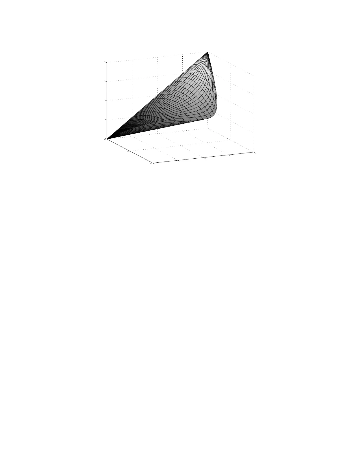
LIDS T ec hnical Rep ort 2760 1 Separable and Lo w-Rank Con tin uous Games Noah D. Stein, Asuman Ozdaglar, and P ablo A. P arrilo ∗ † Octob er 24, 2018 Abstract In this pap er, w e study nonzero-sum separable games, which are contin uous games whose pa y offs tak e a sum-of-pro ducts form. Included in this sub class are all finite games and p olynomial games. W e inv estigate the structure of equilibria in separable games. W e sho w that these games admit finitely supp orted Nash equilibria. Motiv ated b y the b ounds on the supp orts of mixed equilibria in tw o-pla y er finite games in terms of the ranks of the pa y off matrices, we define the notion of the rank of an n -play er con tin uous game and use this to pro vide b ounds on the cardinalit y of the supp ort of equilibrium strategies. W e presen t a general characterization theorem that states that a con tin uous game has finite rank if and only if it is separable. Using our rank results, w e presen t an efficient algorithm for computing appro ximate equilibria of t wo-pla yer separable games with fixed strategy spaces in time p olynomial in the rank of the game. 1 In tro duction The structure and computation of equilibria in games with infinite strategy spaces hav e long b een recognized as complex. Ev en seemingly “go o d” games ma y p ossess only “bad” equi- libria; Gross has constructed an example of a zero-sum game with rational utilit y functions whose unique Nash equilibrium is for eac h pla y er to pla y the Cantor measure [11, 13]. T o a v oid suc h pathologies, Dresher, Karlin, and Shapley in tro duced the class of zero-sum sep- arable games [9, 8, 14, 13]. These are games in whic h each play er’s pa y off can be written as a sum of pro ducts of functions in eac h pla y er’s strategy separately (e.g. as p olynomials), and it is kno wn that every separable game admits a mixed strategy Nash equilibrium that is finitely supp orted, i.e. all play ers randomize ov er a finite num b er of pure strategies. Parrilo has sho wn that Nash equilibria of zero-sum games with p olynomial utility functions can b e computed efficien tly [19]. ∗ Departmen t of Electrical Engineering, Massach usetts Institute of T ec hnology: Cam bridge, MA 02139. nstein@mit.edu , asuman@mit.edu , and parrilo@mit.edu . † This research was funded in part by National Science F oundation grants DMI-0545910 and ECCS- 0621922 and AFOSR MURI subaw ard 2003-07688-1. In this paper, we study nonzero-sum separable games. W e sho w that ev en in the nonzero- sum case, separable games hav e the prop erty that an equilibrium exists in finitely supp orted mixed strategies. W e then characterize the structure of these games and their Nash equilibria, and also prop ose metho ds for computing (exact and appro ximate) equilibria. Our first ma jor con tribution is to define and dev elop the concept of the r ank of a c on- tinuous game , whic h w e use to construct b ounds on the n um b er of strategies play ed in equilibrium. In t w o-pla y er finite games, Lipton et al. hav e recently sho wn that the ranks of the pay off matrices pro vide such a b ound [16]. Our new definition of rank generalizes this one to allow for an arbitrary finite n umber of pla yers (a problem explicitly left op en in [16]) and infinite strategy spaces. W e define the rank of a contin uous game b y introducing an equiv alence relation b et w een mixed strategies called almost p ayoff e quivalenc e . The rank is the dimension of the mixed strategy space mo dulo this equiv alence relation. Lo osely sp eak- ing, low-rank con tinuous games are those where the v ariation in eac h pla y er’s pa y off dep ends only on a low-dimensional pro jection of the mixed strategies of the play ers. F or example in games with p olynomial pa y offs, the rank dep ends on the dimension of a pro jection of the momen t space. W e also sho w that a contin uous game has finite rank if and only if it is separable. This means that little can b e said ab out the structure of equilibria in non-separable contin uous games and highlights the imp ortance of separable games. W e pro vide simple techniques for ev aluating the rank of separable games, whic h w e specialize to games with p olynomial pa y offs and finite games. Our second set of results concern efficien t computation of mixed strategy equilibria in separable games. F or n -pla yer games, w e pro vide a nonlinear optimization formulation, and sho w that the optimal solutions of this problem corresp ond to the (generalized) moments of exact Nash equilibria. This form ulation generalizes the optimization form ulation of Nash equilibria of finite games presen ted b y Ba ¸ sar and Olsder [1]. While the nonlinear optimization formulation for the computation of equilibria is tractable for certain classes of separable games such as zero-sum p olynomial games, the p oten tial non- con v exit y of the optimization problem makes it impractical in other cases. W e therefore supplemen t our computational results for exact mixed strategy equilibria with new meth- o ds for computing appro ximate mixed strategy equilibria. Using our rank results describ ed ab o v e, we can link the computation of mixed strategy equilibria to the appropriate dis- cretization of the strategy space in to finite actions. F or tw o-p erson separable games, this yields an efficient algorithm for computing approximate mixed strategy equilibria in time p olynomial in the rank of the game. This algorithm searches for finitely supported approxi- mate equilibria b y enumerating all possible supp orts, and relies on the fact that the search can b e limited to supp orts of size b ounded by the rank of the game. F or tw o-play ers, the set of equilibria for a giv en supp ort can b e describ ed b y linear equations and inequalities 1 . Our w ork is related to a n um b er of literatures. There has b een considerable work on the computation of equilibria in finite games. Lemk e and Ho wson giv e a path-following al- 1 With more than tw o pla yers this description is no longer linear (or conv ex), so this algorithm do es not generalize to n -play er games with n > 2. 2 gorithm for t w o-pla y er finite games whic h can b e viewed as the simplex metho d for linear programming op erating with a different piv oting rule [15]. T o find equilibria of games with more pla y ers, Scarf constructs a simplicial sub division algorithm whic h also works for more general fixed p oin t problems [22]. These metho ds rely on the p olyhedral structure of the mixed strategy spaces of finite games, therefore they seem unlikely to generalize to con tin- uous/separable games. F or a survey of algorithms whic h compute equilibria of finite games, see [17]. Another gro wing literature has b een in v estigating the complexit y of computing mixed strategy Nash equilibria of finite games. Dask alakis, Goldb erg, and Papadimitriou settle this question for finite normal form games with four or more pla y ers, showing that the problem of computing a single Nash equilibrium is PP AD-complete [6]. In essence this means that it is computationally equiv alent to a n umber of other fixed p oin t problems which are believed to b e computationally difficult. These problems share the feature that a solution can b e prov en to exist, but the known pro ofs of existence are inefficien t; for more ab out the complexity class PP AD, see [18]. Dask alakis and Papadimitriou later improv e this result b y pro ving PP AD- completeness in the case of three play ers [7]. Chen and Deng also prov e this indep endently [4] and complete this line of work b y proving PP AD-completeness for tw o play ers [5]. In this literature, there has b een no w ork on con tin uous games. Our w ork is most closely related to the w ork of Lipton et al. [16], who consider t w o- pla y er finite games and pro vide bounds on the supp ort of equilibrium strategies using the ranks of the pay off matrices of the play ers. Since finite games are a sp ecial case of separable games, our results on the cardinality of the supp ort of equilibrium strategies generalize theirs b y allowing for an arbitrary finite num b er of pla yers as well as infinite strategy sets and a broader class of pa y off functions. Lipton et al. also in v estigate computing appro ximate equilibria in t wo-pla yer finite games and presen t the first algorithm for computing approximate equilibria whic h is quasi-p olynomial in the num b er of strategies [16]. The rank of a separable game measures the complexit y of the pay offs, and in the case of a finite game it is b ounded by the n um b er of strategies. Therefore in finite games the complexity of the pa yoffs and the complexity of the strategy spaces do not v ary indep endently; the effects of these parameters on the running time of algorithms cannot be distinguished. Ho w ev er, for games with infinite strategy sets the rank can b e v aried arbitrarily while the strategy set is held fixed. This allo ws us to construct an algorithm for computing appro ximate equilibria in t wo-pla yer separable games with fixed (infinite) strategy spaces and show that it has a p olynomial dep endence on the rank. Since w e assume the strategy space is fixed and consider general separable games rather than only finite games, our algorithm is not directly comparable to that of Lipton et al. [16]. Nonethe- less it is interesting on its own since no algorithm for computing approximate equilibria of finite games is kno wn whic h has p olynomial dep endence on the complexit y of the game. Our w ork is also related to that of Kannan and Theobald, who study a differen t notion of rank in t wo-pla yer finite games [12]. They tak e an algorithmic p ersp ective and view zero-sum games as the simplest type of games. T o generalize these, they prop ose a hierarch y of classes of t w o-pla y er finite games in whic h the rank of the sum R + C of the pa y off matrices is b ounded 3 b y a constant k ; the case k = 0 corresponds to zero-sum games. F or fixed k , they show that appro ximate Nash equilibria of tw o-play er finite games can b e computed in time polynomial in the description length for the game. This algorithm relies on an approximation result for quadratic programming due to V av asis [25] which dep ends on the p olyhedral structure of the problem. It is conceiv able that this tec hnique may apply to p olynomial games if the appro ximation technique can b e extended to this more general algebraic setting, but we do not do so here. The rest of this pap er is organized as follows. In Section 2 we define separable games and pro v e some of their basic properties. Then in Section 3 w e define the rank of a con tinuous game and use this definition to b ound the cardinalit y of the supp ort of Nash equilibria. W e present a c haracterization theorem for separable games which in particular shows that within the class of contin uous games, the lo w-rank results in this paper cannot be extended past separable games. W e pro vide a simple formula for computing the rank of arbitrary separable games, whic h w e specialize for finite and p olynomial games. In Section 4 we discuss computation of Nash equilibria and appro ximate equilibria. W e close with conclusions and directions for future w ork. 2 Basic Theory of Separable Games W e first in tro duce the notational con v en tions and the basic terminology used throughout the pap er. Subscripts refer to play ers, while superscripts are reserved for other indices, rather than exp onen ts. If S j are sets for j = 1 , . . . , n then S = Π n j =1 S j and S − i = Π j 6 = i S j . The n -tuple s and the ( n − 1)-tuple s − i are formed from the p oints s j similarly . Giv en a subset S of a vector space, w e use the notation span S , aff S , con v S , and S to denote the span, affine h ull, con v ex h ull, and closure of the set S , resp ectively . W e denote the transp ose of a matrix M by M 0 . Definition 2.1. An n -play er contin uous game consists of a pure strategy space C i whic h is a nonempty compact metric space and a contin uous utility or pa y off function u i : C → R for each play er i = 1 , . . . , n . Throughout, ∆ i will denote the space of Borel probabilit y measures σ i o v er C i , referred to as mixed strategies , and the u i will b e extended from C to ∆ by expectation, defining u i ( σ ) = Z C u i ( s ) dσ, where the n -tuple σ = ( σ 1 , . . . , σ n ) is iden tified with the pro duct measure σ 1 × · · · × σ n . Definition 2.2. An n -play er separable game is an n -play er contin uous game with utility functions u i : C → R taking the form u i ( s ) = m 1 X j 1 =1 · · · m n X j n =1 a j 1 ··· j n i f j 1 1 ( s 1 ) · · · f j n n ( s n ) , (1) 4 where a j 1 ··· j n i ∈ R and the f j i : C i → R are contin uous. Two imp ortan t sp ecial cases are the finite games in whic h the C i are finite and the u i are arbitrary and the p olynomial games in which the C i are compact in terv als in R and the u i are p olynomials in the s j . When it is con v enien t to do so, and alwa ys for p olynomial games, we will b egin the summations in (1) at j i = 0. F or polynomial games we can then use the con v en tion that f j i ( s i ) = s j i , where the sup erscript on the righ t hand side denotes an exp onent rather than an index. Example 2.3 . Consider a tw o play er game with C 1 = C 2 = [ − 1 , 1] ⊂ R . Letting x and y denote the pure strategies of pla y ers 1 and 2, resp ectiv ely , w e define the utilit y functions u 1 ( x, y ) = 2 xy + 3 y 3 − 2 x 3 − x − 3 x 2 y 2 and u 2 ( x, y ) = 2 x 2 y 2 − 4 y 3 − x 2 + 4 y + x 2 y . (2) This is a p olynomial game, and we will return to it p erio dically to apply the results presen ted. In particular, we will sho w using classical techniques that this game m ust ha v e a Nash equilibrium in whic h each pla y er randomizes o v er a set of cardinalit y at most 5. W e will then apply our new rank results (see Theorem 3.3) to reduce this b ound to 2 for the first pla y er and 4 for the second pla y er. Let V i denote the space of all finite-v alued signed measures (henceforth simply called measures) on C i , which can b e identified with the dual of the Banach space C ( C i ) of all con tin uous real-v alued functions on C i endo w ed with the sup norm. Throughout, we will use the w eak* top ology on V i , whic h is the w eak est topology such that whenev er f : C i → R is a con tin uous function, σ 7→ R f dσ is a contin uous linear functional on V i . W e can extend the utilit y functions of a con tinuous game to all of V in the same wa y they are extended from C to ∆, yielding a m ultilinear functional on V . F or a fixed separable game w e can extend the f j i from C i to V i similarly , yielding the so-called generalized moment functionals, so (1) holds with s replaced by σ ∈ V . In p olynomial games f j i ( s i ) = s j i so the generalized moment functionals are just the classical moment functionals. W e will abuse notation and identify the elemen ts of C i with the atomic measures in ∆ i , so C i ⊆ ∆ i ⊂ V i . Note that conv C i and span C i are the set of all finitely supp orted probability measures and the set of all finitely supported finite signed measures, resp ectiv ely . The follo wing are standard results (see [20] and [21]). Prop osition 2.4. (a) The sets C i and ∆ i ar e we ak* c omp act. (b) The we ak* closur es of conv C i and span C i ar e ∆ i and V i , r esp e ctively. (c) The we ak* top olo gy makes V i a Hausdorff top olo gic al ve ctor sp ac e. W e next define three notions of equiv alence b etw een tw o measures, which allo w us to exhibit simplifications in the structure of Nash equilibria in separable games. 5 Definition 2.5. Two measures σ i , τ i ∈ V i are • momen t equiv alen t if f j i ( σ i ) = f j i ( τ i ) for all j (representation-dependent and only defined for separable games). • pa y off equiv alent if u j ( σ i , s − i ) = u j ( τ i , s − i ) for all j and all s − i ∈ C − i . • almost pay off equiv alent if u j ( σ i , s − i ) = u j ( τ i , s − i ) for all j 6 = i and all s − i ∈ C − i . Note that in separable games moment equiv alence implies pa y off equiv alence and in all con tin uous games pa y off equiv alence implies almost pa yoff equiv alence. Since the f j i and u j are linear and m ultilinear functionals on V i and V , respectively , these equiv alence relations can b e expressed in terms of (p oten tially infinitely man y) linear constrain ts on σ i − τ i . Definition 2.6. Let 0 denote the zero measure in V i and define • W i = { measures momen t equiv alen t to 0 } , • X i = { measures pa y off equiv alen t to 0 } , • Y i = { measures almost pa y off equiv alen t to 0 } . Then W i ⊆ X i ⊆ Y i , and σ i − τ i ∈ X i if and only if σ i is pay off equiv alent to τ i , etc. F urthermore, the subspaces X i and Y i are represen tation-indep enden t and well-defined for any con tin uous game, separable or not. Note that these subspaces are given by the in tersection of the k ernels of (p otentially infinitely many) con tin uous linear functionals, hence they are closed. W e will analyze separable games b y considering the quotien ts of V i b y these subspaces, i.e. V i mo d these three equiv alence relations. T o a v oid defining excessively many sym b ols let ∆ i /W i denote the image of ∆ i in V i /W i and so forth. F or a concrete example of these sets see the discussion at end of this section, and in particular Figure 1. The follo wing theorem presen ts a fundamen tal result ab out separable games. It sho ws that regardless of the c hoices of the other play ers, eac h pla yer is free to restrict his c hoice of strategies to a particularly simple class of mixed strategies, namely those whic h only assign p ositiv e probabilit y to a finite num b er of pure strategies. F urthermore, a b ound on the n um b er of strategies needed can b e easily computed in terms of the structure of the game. This theorem can b e pro v en b y a separating hyperplane argument as applied to zero-sum separable games b y Karlin [13], but here w e giv e a new top ological argumen t. Theorem 2.7. In a sep ar able game every mixe d str ate gy σ i is moment e quivalent to a finitely- supp orte d mixe d str ate gy τ i with | supp( τ i ) | ≤ m i + 1 . Mor e over, if σ i is c ountably-supp orte d τ i c an b e chosen with supp( τ i ) ⊂ supp( σ i ) . Pr o of. Note that the map f i : σ i 7→  f 1 i ( σ i ) , . . . , f m i i ( σ i )  (3) 6 is linear and con tin uous. Therefore f i (∆ i ) = f i  con v C i  ⊆ f i (con v C i ) = conv f i ( C i ) = conv f i ( C i ) = f i (con v C i ) ⊆ f i (∆ i ) . The first three steps follow from Proposition 2.4, contin uity of f i , and linearit y of f i , resp ec- tiv ely . The next equality holds because con v f i ( C i ) is compact, b eing the conv ex h ull of a compact subset of a finite-dimensional space. The final t wo steps follow from the linearit y of f i and the con tainmen t con v C i ⊆ ∆ i . Hence, we ha ve f i (∆ i ) = conv f i ( C i ) = f i (con v C i ) . This shows that any mixed strategy is momen t equiv alent to a finitely-supp orted mixed strategy . Applying Carath´ eo dory’s theorem [2] to the set con v f i ( C i ) ⊂ R m i yields the uniform b ound. Since a countable conv ex com bination of p oints in a b ounded subset of R m i can alw a ys b e written as a finite conv ex combination of at most m i + 1 of those p oints, the final claim follo ws. F or the rest of the pap er w e will study the Nash equilibria of (nonzero-sum) separable games, whic h are defined for arbitrary con tin uous games as follo ws. Definition 2.8. A mixed strategy profile σ is a Nash equilibrium if u i ( τ i , σ − i ) ≤ u i ( σ ) for all i and all τ i ∈ ∆ i . Com bining Theorem 2.7 with Glicksberg’s result [10] that ev ery contin uous game has a Nash equilibrium yields the follo wing: Corollary 2.9. Every sep ar able game has a Nash e quilibrium in which player i mixes among at most m i + 1 pur e str ate gies. Example 2.3 (cont’d) . Apply the standard definition of the f j i to the p olynomial game with pa y offs giv en in (2). The set of momen ts ∆ i /W i ∼ = f i (∆ i ) as describ ed in Theorem 2.7 is sho wn in Figure 1 with the zeroth moment omitted (it is identically unit y). In this case the set of momen ts is the same for b oth pla yers. The space V i /W i = f i ( V i ) is a four-dimensional real vector space, and Figure 1 shows a subset of the pro jection of V i /W i on to its final three co ordinates. The set C i /W i = f i ( C i ) of momen ts due to pure strategies is the curve traced out by the v ector (1 , x, x 2 , x 3 ) as x v aries from − 1 to 1. Since the first coordinate is omitted in the figure, this can b e seen as the sharp edge which go es from ( − 1 , 1 , − 1) through (0 , 0 , 0) to (1 , 1 , 1). As sho wn in the pro of of Theorem 2.7, f i (∆ i ) is exactly the con v ex hull of this curv e. F or eac h pla y er the range of the indices in (1) is 0 ≤ j i ≤ 3, so by Corollary 2.9, this game has an equilibrium in which eac h play er mixes among at most 4 + 1 = 5 pure strategies. T o pro duce this b ound, we hav e not used an y information ab out the pay offs except for the degree of the p olynomials. Ho w ev er, notice that there is extra structure here to b e exploited. F or example, u 2 dep ends on the exp ected v alue R x 2 dσ 1 ( x ), but not on R xdσ 1 ( x ) or R x 3 dσ 1 ( x ). In particular, pla yer 2 is indifferent b et w een the tw o strategies ± x of play er 1 7 −1 −0.5 0 0.5 1 0 0.5 1 −1 −0.5 0 0.5 1 f i 1 ( σ i ) = ∫ x d σ i (x) f i 2 ( σ i ) = ∫ x 2 d σ i (x) f i 3 ( σ i ) = ∫ x 3 d σ i (x) Figure 1: The space f i (∆ i ) ∼ = ∆ i /W i of p ossible momen ts for either pla yer’s mixed strategy under the pa y offs giv en in (2) due to a measure σ i on [ − 1 , 1]. The zeroth moment, which is iden tically unit y , has b een omitted. for all x , insofar as this choice do es not affect his pa yoff (though it do es affect what strategy profiles are equilibria). In the follo wing section, w e will presen t impro v ed b ounds on the n um b er of strategies play ed in an equilibrium whic h take these simplifications into accoun t in a systematic manner. 3 The Rank of a Con tin uous Game In this section, w e in tro duce the notion of the r ank of a c ontinuous game . W e use this notion to provide improv ed bounds on the cardinalit y of the support of the equilibrium strategies for a separable game. W e also pro vide a characterization theorem whic h states that a contin uous game has finite rank if and only if it is separable, th us sho wing that separable games are the largest class of contin uous games to whic h low-rank arguments apply (see subsection 3.2). W e conclude this section b y sho wing how to compute the rank of a separable game in Subsection 3.3, which ma y b e read indep endently of the section on the c haracterization theorem. Our main result on b ounding the supp ort of equilibrium strategies generalizes the fol- lo wing theorem of Lipton et al. [16] to arbitrary separable games, thereby removing the t w o-pla y er assumption and weak ening the restriction that the strategy spaces be finite. The pro of given in [16] is essentially an algorithmic v ersion of Carath´ eo dory’s theorem. Here w e provide a shorter nonalgorithmic pro of which illustrates some of the ideas to b e used in 8 establishing the extended v ersion of the theorem. Theorem 3.1 (Lipton et al. [16]) . Consider a two-player finite (i.e. bimatrix) game define d by matric es R and C of p ayoffs to the r ow and c olumn player, r esp e ctively. L et σ b e a Nash e quilibrium of the game. Then ther e exists a Nash e quilibrium τ which yields the same p ayoffs to b oth players as σ , but in which the c olumn player mixes among at most rank R + 1 pur e str ate gies and the r ow player mixes among at most rank C + 1 pur e str ate gies. Pr o of. Let r and c be probabilit y column v ectors corresponding to the mixed strategies of the ro w and column play ers in the giv en equilibrium σ . Then the pay offs to the row and column pla yers are r 0 Rc and r 0 C c . Since c is a probability v ector, w e can view Rc as a con vex com bination of the columns of R . These columns all lie in the column span of R , whic h is a v ector space of dimension rank R . By Carath ´ eo dory’s theorem, w e can therefore write an y con v ex com bination of these v ectors using only rank R + 1 terms [2]. That is to sa y , there is a probability vector d suc h that Rd = Rc , d has at most rank R + 1 nonzero en tries, and a comp onen t of d is nonzero only if the corresp onding comp onen t of c w as nonzero. Since r w as a b est resp onse to c and Rc = Rd , r is a b est resp onse to d . On the other hand, since ( r , c ) w as a Nash equilibrium c m ust hav e been a mixture of b est responses to r . But d only assigns positive probability to strategies to whic h c assigned positive probability . Th us d is a best resp onse to r , so ( r , d ) is a Nash equilibrium which yields the same pay offs to b oth play ers as ( r, c ), and d only assigns p ositive probabilit y to rank R + 1 pure strategies. Applying the same procedure to r we could find an s which only assigns p ositive probabilit y to rank C + 1 pure strategies and such that ( s, d ) is a Nash equilibrium with the same pa yoffs to b oth pla y ers as ( r , c ). W e will sho w in the follo wing subsection that our extension of this theorem pro vides a sligh tly tighter b ound of rank R instead of rank R + 1 (resp ectively for C ) in some cases, dep ending on the structure of R and C . This can b e seen directly from the pro of given here. W e considered con v ex combinations of the columns of R and noted that these all lie in the column span of R . In fact, they all lie in the affine h ull of the set of columns of R . If this affine h ull do es not include the origin, then it will hav e dimension rank R − 1. The rest of the pro of go es through using this affine h ull instead of the column span, and so in this case w e get a b ound of rank R on the num b er of strategies pla y ed with positive probabilit y b y the ro w pla yer. Alternatively , the dimension of the affine hull can b e computed directly as the rank of the matrix given b y subtracting a fixed column of R from all the other columns of R . 3.1 Bound on the Supp ort of Equilibrium Strategies By comparing the t wo-pla yer case of (1) with the singular v alue decomp osition for matrices, separable games can b e thought of as games of “finite rank.” Now we will define the rank of a con tin uous game precisely and use it to give a b ound on the cardinality of the supp ort of equilibrium strategies, generalizing Corollary 2.9 and Theorem 3.1. The primary to ol will b e 9 the notion of almost pa y off equiv alence from Definition 2.5. In what follo ws, the dimension of a set will refer to the dimension of its affine h ull. Definition 3.2. The rank of a con tin uous game is defined to b e the n -tuple ρ = ( ρ 1 , . . . , ρ n ) where ρ i = dim ∆ i / Y i . A game is said to hav e finite rank if ρ i < ∞ for all i . Since W i ⊆ Y i and V i /W i is finite-dimensional for any separable game (see the pro of of Theorem 2.7), it is clear that separable games ha v e finite rank, and furthermore that ρ i ≤ m i for all i . In subsection 3.2 w e show that all games of finite rank are also separable, so the t w o conditions are equiv alent. Unlike the m i , the rank is defined for all con tin uous games and is represen tation-indep enden t. W e define the rank of a game in terms of almost pay off equiv alence of mixed strategies b y means of the subspace Y i . This notion of equiv alence b et w een tw o strategies for a given pla y er means that no matter what the other pla y ers do, their pay offs will not enable them to distinguish these tw o strategies. The use of this equiv alence relation reflects the fact that at a (mixed strategy) Nash equilibrium, the pa yoff to a play er is equalized among all pure strategies whic h he pla ys with p ositive probabilit y . Therefore the play er is free to switc h to an y other mixed strategy supported on the same pure strategies, as long as the change do es not affect the other pla yers, and the resulting strategy profile will remain a Nash equilibrium. Using the rank of a game, Corollary 2.9 and Theorem 3.1 can no w b e impro ved as follo ws: Theorem 3.3. Given an e quilibrium σ of a sep ar able game with r ank ρ , ther e exists an e quilibrium τ such that e ach player i mixes among at most ρ i + 1 pur e str ate gies and u i ( σ ) = u i ( τ ) . If dim ∆ i /X i = 1 and the metric sp ac e C i is c onne cte d, then this b ound c an b e impr ove d so that τ i is a pur e str ate gy. Pr o of. By Theorem 2.7, w e can assume without loss of generalit y that eac h play er’s mixed strategy σ i is finitely supp orted. Fix i , let ψ i : V i → V i / Y i denote the canonical pro jection transformation and let σ i = P j λ j s j i b e a finite conv ex combination of pure strategies. By linearit y of ψ i w e ha v e ψ i ( σ i ) = X j λ j ψ i ( s j i ) . Carath ´ eo dory’s theorem states that (renum b ering the s j i and adding some zero terms if necessary) w e can write ψ i ( σ i ) = ρ i X j =0 µ j ψ i ( s j i ) , a con v ex combination p otentially with few er terms. Let τ i = P ρ i j =0 µ j s j i . Then ψ i ( σ i ) = ψ i ( τ i ). Since σ w as a Nash equilibrium, and σ i is almost pa yoff equiv alent to τ i , σ j is a best resp onse to ( τ i , σ − i,j ) for all j 6 = i . On the other hand σ i w as a mixture among b est responses to the mixed strategy profile σ − i , so the same is true of τ i , making it a b est resp onse to σ − i . Th us ( τ i , σ − i ) is a Nash equilibrium. 10 If dim ∆ i /X i = 1 and C i is connected, then C i /X i is connected, compact, and one- dimensional, i.e. it is an interv al. Therefore it is con v ex, so ∆ i /X i = conv( C i /X i ) = C i /X i . This implies that there exists a pure strategy s i whic h is pa y off equiv alent to σ i , so w e ma y tak e τ i = s i and ( τ i , σ − i ) is a Nash equilibrium. Beginning with this equilibrium and rep eating the ab o v e steps for eac h play er in turn completes the construction of τ and the final statemen t of the theorem is clear. While the preceding theorem w as the original reason for our choice of the definition of ρ , the definition turns out to hav e other interesting prop erties which we study below. The follo wing alternativ e c haracterization of the rank of a con tin uous game is more concrete than the definition giv en ab o ve. This theorem simplifies the pro ofs of many rank-related results and will b e applied to the problem of computing the rank of separable games in Subsection 3.3. Theorem 3.4. The r ank ρ i for player i in a c ontinuous game is given by the smal lest r i such that ther e exist c ontinuous functions g k i : C i → R and h k i,j : C − i → R which satisfy u j ( s ) = h 0 i,j ( s − i ) + r i X k =1 g k i ( s i ) h k i,j ( s − i ) (4) for al l s ∈ C and j 6 = i ( ρ i = ∞ if and only if no such r epr esentation exists). F urthermor e, the minimum value of r i = ρ i is achieve d by functions g k i ( s i ) of the form u j ( s i , s − i ) for some s − i ∈ C − i and j 6 = i and functions h k i,j ( s − i ) of the form R u j ( · , s − i ) dσ i for some σ i ∈ V i . Pr o of. Throughout the pro of w e will automatically extend an y functions g k i : C i → R to all of V i in the canonical w a y . Supp ose w e are given a representation of the form (4). Let g i : C i → R r i b e defined b y g i ( s i ) = ( g 1 i ( s i ) , . . . , g r i i ( s i )). By definition, ρ i is the dimension of ∆ i / Y i . Let Z i denote the subspace of V i parallel to ∆ i , i.e. the space of all signed measures σ i suc h that R σ i = 0. Then ρ i = dim Z i / ( Z i ∩ Y i ). By (4) any signed measure whic h is in Z i and in k er g i is almost pa yoff equiv alent to the zero measure, so Z i ∩ k er g i ⊆ Z i ∩ Y i and therefore ρ i = dim Z i / ( Z i ∩ Y i ) ≤ dim Z i / ( Z i ∩ ker g i ) = dim g i ( Z i ) ≤ r i . It remains to show that if ρ i < ∞ then there exists a represen tation of the form (4) with r i = ρ i . Recall that Y i is defined to b e Y i = \ j 6 = i s − i ∈ C − i k er u j ( · , s − i ) where u j ( · , s − i ) is interpreted as a linear functional on V i . Since ρ i = dim Z i / ( Z i ∩ Y i ), w e can c ho ose ρ i linear functionals, call them g 1 i , . . . , g ρ i i , from the collection of functionals whose in tersection forms Y i , such that Z i ∩ Y i = Z i ∩ ker g i , where g i = ( g 1 i , . . . , g ρ i i ) as ab o v e. W e cannot choose a smaller collection of linear functionals and ac hiev e Z i ∩ Y i = Z i ∩ ker g i , b ecause ρ i = dim Z i / ( Z i ∩ Y i ). Note that Z i ∩ ker g i = k er (1 , g 1 i , . . . , g ρ i i ) where 1 is the linear 11 functional 1( σ i ) = R dσ i . Therefore no functional can b e remo v ed from the list (1 , g i ) = (1 , g 1 i , . . . , g ρ i i ) without affecting the kernel of the transformation (1 , g i ), so the functionals 1 , g 1 i , . . . , g ρ i i are linearly indep enden t. This means that any of the linear functionals u j ( · , s − i ) (the in tersection of whose k ernels yields Y i ) can b e written uniquely as a linear combination of the functionals 1 , g 1 i , . . . , g ρ i i . That is to sa y , there are unique functions h k i,j suc h that (4) holds with the functions g k i constructed here and r i = ρ i . The g k i are contin uous by construction, so to complete the pro of we must show that the functions h k i,j are contin uous as w ell. Since the functionals 1 , g 1 i , . . . , g ρ i i are linearly indep endent, we can choose a measure σ k i ∈ V i whic h makes the k th of these functionals ev aluate to unity and all the others zero. Substituting these v alues in to (4) sho ws that h k i,j ( s − i ) = R u j ( · , s − i ) dσ k i . Since u j is contin uous, h k i,j is therefore also con tin uous. Note that in the statemen t of Theorem 3.4 w e hav e distinguished the comp onen t h 0 i,j ( s − i ) in u j . W e ha ve shown that this distinction follo ws from the definition of ρ i , but there is also an in tuitive game theoretic reason wh y this separation is natural. As men tioned abov e, ρ i is in tended to capture the n um b er of essen tial degrees of freedom that pla y er i has in his c hoice of strategy when pla ying a Nash equilibrium. Theorems 3.3 and 3.4 together show that play er i only needs to tak e the other pla y ers’ utilities into accoun t to compute this n um b er, and not his own. But pla y er i is only concerned with the other play ers’ utilities insofar as his o wn strategic c hoice affects them. The function h 0 i,j ( s − i ) captures the part of pla y er j ’s utilit y whic h do es not dep end on play er i ’s strategy , so whether this function is zero or not it has no effect on the rank ρ i . Also note that while Theorem 3.4 giv es decompositions of the utilities in terms of the ρ i , it is not in general p ossible to summarize all these decomp ositions b y writing the utilities in the form (1) with m i = ρ i for all i . F or a trivial counterexample, consider any game in whic h u i ( s ) = h 0 i ( s − i ) is indep enden t of s i for all i . Then Theorem 3.4 implies that ρ i = 0 for all i , but the utilities are nonzero so w e cannot tak e m i = 0 in (1) for any i . W e close this subsection with an application. If a submatrix is formed from a matrix b y “sampling,” i.e. selecting a subset of the ro ws and columns, the rank of the submatrix is b ounded by the rank of the original matrix. Theorem 3.4 sho ws that the same is true of con tin uous games, b ecause a factorization of the form (4) for a game immediately provides a factorization for an y smaller game produced b y restricting the play ers’ choices of strategies. Corollary 3.5. L et ( { C i } , { u i } ) b e a c ontinuous game with r ank ρ and ˜ C i b e a nonempty c omp act subset of C i for e ach i , with ˜ u i = u i   ˜ C . L et ˜ ρ denote the r ank of the game ( { ˜ C i } , { ˜ u i } ) . Then we have ˜ ρ i ≤ ρ i for al l i . Definition 3.6. The game ( { ˜ C i } , { ˜ u i } ) in Corollary 3.5 is called a sampled game or a sampled version of ( { C i } , { u i } ). Note that if we take ˜ C i to b e finite for eac h i , then the sampled game is a finite game. If the original game is separable and hence has finite rank, then Corollary 3.5 yields a uniform b ound on the complexity of finite games which can arise from this game by sampling. This 12 fact is applied to the problem of computing approximate equilibria in Section 4 b elo w. Finally , note that there are other kinds of b ounds on the cardinalit y of the supp ort of equilibria (e.g., for special classes of p olynomial games as studied by Karlin [13]) whic h do not share this sampling prop ert y . 3.2 Characterizations of separable games In this section we presen t a c haracterization theorem for separable games. W e also provide an example that sho ws that the assumptions of this theorem cannot b e w eak ened. Theorem 3.7. F or a c ontinuous game, the fol lowing ar e e quivalent: 1. The game is sep ar able. 2. The game has finite r ank. 3. F or e ach player i , every c ountably supp orte d mixe d str ate gy σ i is almost p ayoff e quiva- lent to a finitely supp orte d mixe d str ate gy τ i with supp( τ i ) ⊂ supp( σ i ) . T o prov e that finite rank implies separability we rep eatedly apply Theorem 3.4. The pro of that the technical condition (3) implies (2) uses a linear algebraic argumen t to sho w that span C i / Y i is finite dimensional and then a top ological argumen t along the lines of the pro of of Theorem 2.7 to sho w that V i / Y i is also finite dimensional. After the pro of of Theorem 3.7 w e will giv e an explicit example of a game in whic h all mixed strategies are pay off equiv alen t to pure strategies, but for which the con tainmen t supp( τ i ) ⊂ supp( σ i ) in condition (3) fails. In ligh t of Theorem 3.7 this will show that the constructed game is nonseparable and that the containmen t supp( τ i ) ⊂ supp( σ i ) cannot be dropp ed from condition (3), ev en if the other assumptions are strengthened. Pr o of. (1 ⇒ 3) This was pro ven in Theorem 2.7. (1 ⇒ 2) This follo ws from the pro of of Theorem 2.7. (2 ⇒ 1) W e will pro ve this by induction on the n umber of play ers n . When n = 1 the statemen t is trivial and the case n = 2 follo ws immediately from Theorem 3.4. Supp ose w e hav e an n -play er con tin uous game with ρ i < ∞ for all i and that we ha v e prov en that ρ i < ∞ for all i implies separabilit y for ( n − 1)-pla y er games. By fixing an y signed measure σ n ∈ V n w e can form an ( n − 1)-play er contin uous game from the given game b y remo ving the n th pla y er and in tegrating all pa yoffs of play ers i < n with resp ect to σ n , yielding a new game with pa y offs ˜ u i ( s − n ) = R u i ( s n , s − n ) dσ n ( s n ). F rom the definition of Y i , it is clear that Y i ⊆ ˜ Y i for all 1 ≤ i < n . Therefore ˜ ρ i = dim ∆ i / ˜ Y i ≤ dim ∆ i / Y i = ρ i < ∞ for 1 ≤ i < n so the ( n − 1)-play er game has finite rank. By the induction h yp othesis, that means that the function ˜ u 1 is a separable function of the strategies s 1 , . . . , s n − 1 . Theorem 3.4 states that there exist con tinuous functions g k n and h k n, 1 suc h that u 1 ( s ) = h 0 n, 1 ( s − n ) + ρ n X k =1 g k n ( s n ) h k n, 1 ( s − n ) (5) 13 where h k n, 1 = R u 1 ( s ) dσ k n for some σ k n ∈ V n . Therefore by choosing σ n appropriately w e can mak e ˜ u 1 = h k n, 1 for any k , so h k n, 1 ( s − n ) is a separable function of s 1 , . . . , s n − 1 for all k . By (5) u 1 is a separable function of s 1 , . . . , s n . The same argument w orks for all the u i so the giv en game is separable and the general case is true b y induction. (3 ⇒ 2) Let ψ i : V i → V i / Y i b e the canonical pro jection transformation. First w e will pro v e that span ψ i ( C i ) is finite dimensional. It suffices to pro v e that for every coun table subset ˜ C i = { s 1 i , s 2 i , . . . } ⊆ C i , the set ψ i ( ˜ C i ) is linearly dep endent. Let { p k } b e a sequence of p ositiv e reals summing to unit y . Define the mixed strategy σ i = ∞ X k =1 p k s k i . By assumption there exists an M and q 1 , . . . , q M ≥ 0 summing to unity suc h that ψ i ( σ i ) = ψ i M X k =1 q k s k i ! = M X k =1 q k ψ i ( s k i ) . Let α = ∞ X k = M +1 p k > 0 and define the mixed strategy τ i = ∞ X k = M +1 p k α s k i . Applying the assumption again sho ws that there exist N and r M +1 , . . . , r N suc h that ψ i ( τ i ) = ψ i N X k = M +1 r k s k i ! = N X k = M +1 r k ψ i ( s k i ) . Therefore M X k =1 p k ψ i ( s k i ) = ψ i M X k =1 p k s k i ! = ψ i ( σ i − ατ i ) = ψ i ( σ i ) − α ψ i ( τ i ) = M X k =1 q k ψ i ( s k i ) − N X k = M +1 αr k ψ i ( s k i ) , and rearranging terms shows that P M k =1 ( p k − q k ) ψ i ( s k i ) + P N k = M +1 αr k ψ i ( s k i ) = 0. Also P M k =1 ( p k − q k ) = − α < 0, so p k − q k 6 = 0 for some k . Therefore ψ i ( ˜ C i ) is linearly dep enden t, so span ψ i ( C i ) is finite dimensional. Since Y i is closed, V i / Y i is a Hausdorff topological v ector space under the quotien t top ol- ogy and ψ i is con tin uous with resp ect to this top ology [21]. Being finite dimensional, the subspace span ψ i ( C i ) ⊆ V i / Y i is also closed [21]. Thus w e hav e V i / Y i = ψ i ( V i ) = ψ i  span C i  ⊆ ψ i (span C i ) = span ψ i ( C i ) = span ψ i ( C i ) ⊆ V i / Y i 14 where the first step is b y definition, the second follo ws from Prop osition 2.4, the next t w o are by contin uity and linearity of ψ i , and the final tw o are b ecause span ψ i ( C i ) is a closed subspace of V i / Y i . Therefore ρ i = dim ∆ i / Y i ≤ dim V i / Y i = dim span ψ i ( C i ) < ∞ . The follo wing counterexample shows that the con tainmen t supp τ i ⊂ supp σ i is a nec- essary part of condition 3 in Theorem 3.7 by sho wing that there exists a nonseparable con tin uous game in whic h ev ery mixed strategy is pa y off equiv alen t to a pure strategy . Example 3.8 . Consider a tw o-play er game with C 1 = C 2 = [0 , 1] ω , the set of all infinite sequences of reals in [0 , 1], which forms a compact metric space under the metric d ( x, x 0 ) = sup i | x i − x 0 i | i . Define the utilities u 1 ( x, y ) = u 2 ( x, y ) = ∞ X i =1 2 − i x i y i . T o show that this is a contin uous game we m ust sho w that u 1 is contin uous. Assume d ( x, x 0 ) , d ( y , y 0 ) ≤ δ . Then | x i − x 0 i | ≤ δ i and | y i − y 0 i | ≤ δ i , so | u 1 ( x,y ) − u 1 ( x 0 , y 0 ) | =      ∞ X i =1 2 − i ( x i y i − x 0 i y 0 i )      =      ∞ X i =1 2 − i ( x i y i − x 0 i y i + x 0 i y i − x 0 i y 0 i )      ≤ ∞ X i =1 2 − i ( y i | x i − x 0 i | + x 0 i | y i − y 0 i | ) ≤ ∞ X i =1 2 − i (2 δ i ) = 2 ∞ X i =1 2 − i i ! δ. Th us u 1 = u 2 is con tin uous (in fact Lipsc hitz), making this a con tin uous game. Let σ and τ b e mixed strategies for the tw o pla y ers. By the T onelli-F ubini theorem, u 1 ( σ, τ ) = Z u 1 d ( σ × τ ) = ∞ X i =1 2 − i  Z x i dσ   Z y i dτ  . Th us σ is pay off equiv alen t to the pure strategy  R x 1 dσ, R x 2 dσ, . . .  ∈ C 1 and similarly for τ , so this game has the prop ert y that ev ery mixed strategy is pay off equiv alent to a pure strategy . Finally we will sho w that this game is nonseparable. Let e i ∈ C 1 b e the elemen t ha ving comp onen t i equal to unit y and all other comp onents zero. Let { p i } b e a sequence of positive reals summing to unit y and define the probability distribution σ = P ∞ i =1 p i e i ∈ ∆ 1 . Supp ose 15 σ were almost pay off equiv alent to some mixture among finitely many of the e i , call it τ = P ∞ i =1 q i e i where q i = 0 for i greater than some fixed N . Let e N +1 b e the strategy for pla y er 2. Then the pay off if play er 1 plays σ is u 2 ( σ, e N +1 ) = Z 2 − ( N +1) x N +1 dσ = 2 − ( N +1) p N +1 . Similarly , if he chooses τ the pa y off is 2 − ( N +1) q N +1 . Since p N +1 > 0 and q N +1 = 0, this con tradicts the assumption that σ and τ are almost pay off equiv alent. Thus condition 3 of Theorem 3.7 do es not hold, so this game is not separable. Therefore the condition that all mixed strategies b e pay off equiv alen t to finitely supp orted strategies do es not imply separabilit y , ev en if a uniform b ound on the size of the supp ort is assumed. Hence the con tainmen t supp τ i ⊂ supp σ i cannot b e remo ved from condition 3 of Theorem 3.7. 3.3 Computing the rank of a separable game In this subsection w e construct a form ula for the rank of an arbitrary separable game and then sp ecialize it to get formulas for the ranks of p olynomial and finite games. F or clarit y of presen tation we first pro ve a b ound on the rank of a separable game which uses an argumen t that is similar to but simpler than the argumen t for the exact formula. While it is p ossible to pro ve all the results in this section directly from the definition ρ i = dim ∆ i / Y i , w e will giv e pro ofs based on the alternative characterization in Theorem 3.4 because they are easier to understand and pro vide more insigh t in to the structure of the problem. Giv en a separable game in the standard form (1), construct a matrix S i,j for pla y ers i and j which has m i columns and Π k 6 = i m k ro ws and whose elemen ts are defined as follows. Lab el eac h ro w with an ( n − 1)-tuple ( l 1 , . . . , l i − 1 , l i +1 , . . . , l n ) suc h that 1 ≤ l k ≤ m k ; the order of the rows is irrelev ant. Lab el the columns l i = 1 , . . . , m i . Each entry of the matrix then corresp onds to an n -tuple ( l 1 , . . . , l n ). The en try itself is giv en by the coefficient a l 1 ··· l n j in the utilit y function u j . Let f i ( s i ) denote the column vector whose comp onents are f 1 i ( s i ) , . . . , f m i i ( s i ) and f − i ( s − i ) denote the ro w vector whose comp onents are the pro ducts f l 1 1 ( s 1 ) · · · f l i − 1 i − 1 ( s i − 1 ) f l i +1 i +1 ( s i +1 ) · · · f l n n ( s n ) ordered in the same w a y as the ( n − 1)-tuples ( l 1 , . . . , l i − 1 , l i +1 , . . . , l n ) w ere ordered ab o v e. Then u j ( s ) = f − i ( s − i ) S i,j f i ( s i ). Example 3.9 . W e introduce a new example game to clarify the subtleties of computing ranks when there are more than tw o play ers; we will return to Example 2.3 later. Consider the three pla y er p olynomial game with strategy spaces C 1 = C 2 = C 3 = [ − 1 , 1] and pa yoffs u 1 ( x, y , z ) = 1 + 2 x + 3 x 2 + 2 y z + 4 xy z + 6 x 2 y z + 3 y 2 z 2 + 6 xy 2 z 2 + 9 x 2 y 2 z 2 u 2 ( x, y , z ) = 7 + 2 x + 3 x 2 + 2 y + 4 xy + 6 x 2 y + 3 z 2 + 6 xz 2 + 9 x 2 z 2 u 3 ( x, y , z ) = − z − 2 xz − 3 x 2 z − 2 y z − 4 xy z − 6 x 2 y z − 3 y z 2 − 6 xy z 2 − 9 x 2 y z 2 (6) 16 where x , y , and z are the strategies of pla y er 1, 2, and 3, resp ectiv ely . Order the functions f l k so that f 1 ( x ) =  1 x x 2  0 and similarly for f 2 and f 3 with x replaced by y and z , resp ectiv ely . If we wish to write down the matrices S 1 , 2 and S 1 , 3 w e must c ho ose an order for the pairwise pro ducts of the functions f l 2 and f l 3 . Here we will choose the order f − 1 ( y , z ) =  1 y y 2 z y z y 2 z z 2 y z 2 y 2 z 2  . W e can write down the desired matrices immediately from the giv en utilities. S 1 , 2 =               7 2 3 2 4 6 0 0 0 0 0 0 0 0 0 0 0 0 3 6 9 0 0 0 0 0 0               , S 1 , 3 =               0 0 0 0 0 0 0 0 0 − 1 − 2 − 3 − 2 − 4 − 6 0 0 0 0 0 0 − 3 − 6 − 9 0 0 0               This yields u 2 ( x, y , z ) = f − 1 ( y , z ) S 1 , 2 f 1 ( x ) and u 3 ( x, y , z ) = f − 1 ( y , z ) S 1 , 3 f 1 ( x ) as claimed. Define S i to b e the matrix with m i columns and ( n − 1)Π j 6 = i m j ro ws which consists of all the matrices S i,j for j 6 = i stac ked vertically (in an y order). In the example ab o v e, S 1 w ould b e the 18 × 3 matrix obtained by placing S 1 , 2 ab o v e S 1 , 3 on the page. Theorem 3.10. The r ank of a sep ar able game is b ounde d by ρ i ≤ rank S i . Pr o of. Using any of a v ariety of matrix factorization techniques (e.g. the singular v alue decomp osition), w e can write S i as S i = rank S i X k =1 v k w k for some column v ectors v k and ro w vectors w k . The vectors v k will ha v e length ( n − 1)Π j 6 = i m j since that is the n umber of ro ws of S i . Because of the definition of S i , w e can break each v k in to n − 1 vectors of length Π j 6 = i m j , one for each pla yer except i , and let v k j b e the v ector corresp onding to pla y er j . Then w e ha v e S i,j = rank S i X k =1 v k j w k for all j 6 = i . Define the linear combinations g k i ( s i ) = w k f i ( s i ) and h k i,j = f − i ( s − i ) v k j , whic h are ob viously con tin uous functions. Then u j ( s ) = f − i ( s − i ) S i,j f i ( s i ) = rank S i X k =1 g k i ( s i ) h k i,j ( s − i ) for all s ∈ C and j 6 = i , so ρ i ≤ rank S i b y Theorem 3.4. 17 Example 3.11 . T o demonstrate the pow er of the b ound in Theorem 3.10 w e will use it to giv e an immediate pro of of Theorem 3.1. Consider any t wo-pla yer finite game, where the first pla y er c ho oses ro ws and the second pla yer c ho oses columns. Let C i = { 1 , . . . , m i } for i = 1 , 2 and let R and C b e the matrices of pa y offs to the ro w and column pla y ers, respectively . W e can then define f l i ( s i ) to b e unit y if s i = l and zero otherwise. This gives u 1 ( s 1 , s 2 ) = f 1 ( s 1 ) 0 Rf 2 ( s 2 ) u 2 ( s 1 , s 2 ) = f 2 ( s 2 ) C 0 f 1 ( s 1 ) so S 1 = C 0 and S 2 = R . Therefore by Theorem 3.10, ρ 1 ≤ rank S 1 = rank C and ρ 2 ≤ rank S 2 = rank R . Substituting these bounds in to Theorem 3.3 yields Theorem 3.1, so w e ha v e in fact generalized the results of Lipton et al. [16]. It is easy to see that there are cases in whic h the bound in Theorem 3.10 is not tight. F or example, this will b e the case (for generic co efficients a j 1 ··· j n i ) if m i ≥ 2 for each i and f k i is the same function for all k . F ortunately w e can use a tec hnique similar to the one used ab ov e to compute ρ i exactly instead of just computing a b ound. T o do so w e need to write the utilities in a sp ecial form. First we add the new function f 1 i ( s i ) ≡ 1 to the list of functions for play er i app earing in the separable representation of the game if this function do es not already appear, relab eling the other f k i as necessary . Next we consider the set of functions { f k j } for each play er j in turn and choose a maximal linearly indep enden t subset. F or pla yers j 6 = i an y such subset will do; for play er i we must include the function whic h is iden tically unity in the chosen subset. Finally w e rewrite the utilities in terms of these linearly indep enden t sets of functions. This is possible because all of the f k j are linear combinations of those whic h app ear in the maximal linearly indep enden t sets. F rom no w on we will assume the utilities are in this form and that f 1 i ( s i ) ≡ 1. Let S i,j and S i b e the matrices S i,j and S i defined abov e, where the bar denotes the fact that w e ha v e put the utilities in this sp ecial form. Let T i b e the matrix S i with its first column remov ed. Note that this column corresp onds to the function f 1 i ( s i ) ≡ 1 which we hav e distinguished ab o v e, and therefore represents the components of the utilities of play ers j 6 = i which do not dep end on pla y er i ’s c hoice of strategy . As mentioned in the note following Theorem 3.4, these comp onents don’t affect the rank. This is exactly the reason that we must remov e the first column from S i in order to compute ρ i . W e will pro ve that ρ i = rank T i , but first we need a lemma. Lemma 3.12. If the functions f 1 j ( s j ) , . . . , f m j j ( s j ) ar e line arly indep endent for al l j , then the set of al l Π n j =1 m j pr o duct functions of the form f k 1 1 ( s 1 ) · · · f k n n ( s n ) is a line arly indep endent set. Pr o of. It suffices to pro v e this in the case n = 2, b ecause the general case follows by induction. W e pro ve the n = 2 case by contradiction. Supp ose the set were linearly dep enden t. Then there w ould exist λ k 1 k 2 not all zero suc h that m 1 X k 1 =1 m 2 X k 2 =1 λ k 1 k 2 f k 1 1 ( s 1 ) f k 2 2 ( s 2 ) = 0 (7) 18 for all s ∈ C . Cho ose l 1 and l 2 suc h that λ l 1 l 2 6 = 0. By the linear indep endence assumption there exists a finitely supp orted signed measure σ 2 suc h that R f k 2 dσ 2 is unity for k = l 2 and zero otherwise. Integrating (7) with resp ect to σ 2 yields m 1 X k 1 =1 λ k 1 l 2 f k 1 1 ( s 1 ) = 0 , con tradicting the linear indep endence assumption for f 1 1 , . . . , f m 1 1 . Theorem 3.13. If the r epr esentation of a sep ar able game satisfies f 1 i ≡ 1 and the set { f 1 j , . . . , f m j j } is line arly indep endent for al l j then the r ank of the game is ρ i = rank T i . Pr o of. The pro of that ρ i ≤ rank T i follo ws ess en tially the same argument as the pro of of Theorem 3.10. W e use the singular v alue decomp osition to write T i as T i = rank T i X k =1 v k w k for some column v ectors v k and ro w vectors w k . The vectors v k will ha v e length ( n − 1)Π j 6 = i m j since that is the n umber of rows of S i . Let v 0 b e the first column of S i , whic h w as remo ved from S i to form T i . Because of the definition of T i and S i , we can break eac h v k in to n − 1 v ectors of length Π j 6 = i m j , one for eac h pla y er except i , and let v k j b e the v ector corresp onding to pla y er j . Putting these definitions together w e get S i,j = v 0 j  1 0 · · · 0  + rank T i X k =1 v k j  0 w k  . Define the linear com binations g k i ( s i ) =  0 w k  f i ( s i ) and h k i,j ( s − i ) = f − i ( s − i ) v k j , which are ob viously con tin uous functions. Then u j ( s ) = f − i ( s − i ) S i,j f i ( s i ) = h 0 i,j ( s − i ) + rank T i X k =1 g k i ( s i ) h k i,j ( s − i ) for all s ∈ C and j 6 = i , so ρ i ≤ rank T i b y Theorem 3.4. T o pro ve the rev erse inequalit y , c ho ose con tinuous functions g k i ( s i ) and h k i,j ( s − i ) suc h that u j ( s ) = h 0 i,j ( s − i ) + ρ i X k =1 g k i ( s i ) h k i,j ( s − i ) holds for all s ∈ C and j 6 = i . By Theorem 3.4 w e can c ho ose these so that g k i ( s i ) is of the form u j ( s i , s − i ) for some s − i ∈ C − i , j 6 = i and h k i,j ( s − i ) is of the form R u j ( · , s − i ) dσ i for some σ i ∈ V i . Substituting these conditions in to equation (1) defining the form of a separable 19 game shows that g k i ( s i ) = w k f i ( s i ) for some row v ectors w k and h k i,j = f − i ( s − i ) v k j for some column v ectors v k j . Define w 0 =  1 0 · · · 0  . Then u j ( s ) = ρ i X k =0 f − i ( s − i ) 0 v k j w k f i ( s i ) for all s ∈ C and j 6 = i . This expresses u j ( s ) as a linear com bination of products of the form f k 1 1 ( s 1 ) · · · f k n n ( s n ). By assumption the sets { f 1 j , . . . , f m j j } are linearly indep endent for all j , and therefore the set of products of the form f k 1 1 ( s 1 ) · · · f k n n ( s n ) is linearly independent by Lemma 3.12. Thus the expression of u j ( s ) as a linear com bination of these pro ducts is unique. But w e also ha ve u j ( s ) = f − i ( s − i ) 0 S i,j f i ( s i ) b y definition of S i,j , so uniqueness implies that S i,j = P ρ i k =0 v k j w k . Let v k b e the vector of length ( n − 1)Π j 6 = i m j formed b y concatenating the v k j in the obvious w a y . Then S i = P ρ i k =0 v k w k . Let ˜ w k b e w k with its first entry remo ved. By definition of T i w e ha ve T i = P ρ i k =0 v k ˜ w k . But w 0 is the standard unit vector with a 1 in the first co ordinate, so ˜ w 0 is the zero v ector and w e ma y therefore remov e the k = 0 term from the sum. Thus T i = P ρ i k =1 v k ˜ w k , whic h pro v es that rank T i ≤ ρ i . As corollaries of Theorem 3.13 we obtain form ulas for the ranks of polynomial and finite games. Corollary 3.14. Consider a game with p olynomial p ayoffs u i ( s ) = m 1 − 1 X j 1 =0 · · · m n − 1 X j n =0 a j 1 ··· j n i s j 1 1 · · · s j n n (8) and c omp act str ate gy sets C i ⊂ R which satisfy the c ar dinality c ondition | C i | > m i for al l i . Then T i is S i with its first c olumn r emove d and ρ i = rank T i . Pr o of. Linear indep endence of the f l i follo ws from the cardinalit y condition and w e ha v e f 0 i ≡ 1, so Theorem 3.13 applies. Example 2.3 (con t’d) . Applying this formula to the utilities in (2) shows that ρ 1 = 1 and ρ 2 = 3. Example 3.9 (cont’d) . Applying this form ula to the utilities in (6) sho ws that in this case ρ 1 = 1 and ρ 2 = ρ 3 = 2. Corollary 3.15. Consider an n -player finite game with str ate gy sets C i = { 1 , . . . , m i } and p ayoff a s 1 ··· s n i to player i if the players play str ate gy pr ofile ( s 1 , . . . , s n ) . The utilities c an b e written as u i ( s ) = m 1 X j 1 =1 · · · m n X j n =1 a j 1 ··· j n i f j 1 1 ( s 1 ) · · · f j n n ( s n ) wher e f l i ( s i ) is unity if s i = l and zer o otherwise. L et S i b e the matrix for player i as define d ab ove and let c 1 , . . . , c m i b e the c olumns of S i . Then we may take T i =  c 2 − c 1 · · · c m i − c 1  and ρ i = rank T i . 20 Pr o of. If w e replace f 1 i with the function which is identically unit y then the linear indep en- dence assumption on the f l k will still b e satisfied, so w e can apply Theorem 3.13. After this replacemen t, the co efficien ts in the new separable represen tation for the game are a j 1 ··· j n k = ( a j 1 ··· j n k if j i = 1, a j 1 ··· j n k − a j 1 ··· j i − 1 1 j i +1 ··· j n k if j i 6 = 1. Therefore if c 1 , . . . , c m i are the columns of S i from the original represen tation of the game w e get S i =  c 1 c 2 − c 1 · · · c m i − c 1  , so T i is as claimed and an application of Theorem 3.13 completes the pro of. 4 Computation of Nash Equilibria and Appro ximate Equilibria In this section, we study computation of exact and approximate Nash equilibria. W e first presen t an optimization formulation for the computation of (exact) Nash equilibria of general separable games. W e sho w that for tw o-pla y er p olynomial games, this formulation has a biaffine ob jective function and linear matrix inequality constrain ts. W e then presen t an algorithm for computing approximate equilibria of t wo-pla yer separable games with infinite strategy sets which follows directly from the results on the rank of games given in Section 3 and compare it with kno wn algorithms for finite games. 4.1 Computing Nash equilibria The momen ts of an equilibrium can in principle b e computed b y nonlinear programming tec hniques using the following generalization of the Nash equilibrium formulation presented b y Ba ¸ sar and Olsder [1]: Prop osition 4.1. The fol lowing optimization pr oblem has optimal value zer o and the vari- ables x in any optimal solution ar e the moments of a Nash e quilibrium str ate gy pr ofile with p ayoff p i to player i : max P n i =1 [ v i ( x ) − p i ] s.t. x i ∈ ∆ i /W i = f i (∆ i ) for al l i v i ( f i ( s i ) , x − i ) ≤ p i for al l i , al l s i ∈ C i The function f i is the moment function define d in (3) and v i is the p ayoff function on the moment sp ac es define d by v i ( f 1 ( σ 1 ) , . . . , f n ( σ n )) = u i ( σ ) . Pr o of. The constrain ts imply that v i ( x ) − p i ≤ 0 for all i , so the ob jective function is b ounded ab o v e b y zero. Giv en an y n -tuple of moments x which form a Nash equilibrium, let p i = v i ( x ) for all i . Then the ob jective function ev aluates to zero and all the constraints are satisfied, b y definition of a Nash equilibrium. Therefore the optimal ob jective function v alue is zero and it is attained at all Nash equilibria. 21 Con v ersely supp ose some feasible x and p ac hiev e ob jectiv e function v alue zero. Then the condition v i ( x ) − p i ≤ 0 implies that v i ( x ) = p i for all i . Also, the final constraint implies that pla y er i cannot achiev e a pa y off of more than p i b y unilaterally changing his strategy . Therefore the momen ts x form a Nash equilibrium. T o compute equilibria b y this metho d, we require an explicit description of the spaces of momen ts ∆ i /W i . W e also require a metho d for describing the pay off p i to pla y er i if he pla ys a b est resp onse to an m − i -tuple of momen ts for the other pla y ers. While it seems doubtful that suc h descriptions could be found for arbitrary f j i , they do exist for t w o-pla y er p olynomial games in which the pure strategy sets are in terv als. In this case they can b e written in terms of linear matrix inequalities as in P arrilo’s treatmen t of the zero-sum case [19]. This yields a problem with biaffine ob jectiv e and linear matrix inequality constrain ts. Example 2.3 (cont’d) . Directly solving this noncon v ex problem with MA TLAB’s fmincon has prov en error-prone, as there app ear to b e man y lo cal minima which are not global. Ho w ev er, w e w ere able to compute the equilibrium measures σ 1 = 0 . 5532 δ ( x + 1) + 0 . 4468 δ ( x − 0 . 1149) , σ 2 = δ ( y − 0 . 7166) (i.e. play er 1 plays the pure strategy x = − 1 with probability 0 . 5532 and so on) for the pa y offs in (2) b y this metho d. 4.2 Computing  -equilibria The difficulties in computing equilibria by general nonconv ex optimization tec hniques suggest the need for more sp ecialized systematic metho ds. As a step tow ard this, we present an algorithm for computing appro ximate Nash equilibria of t wo-pla yer separable games. There are sev eral p ossible definitions of appro ximate equilibrium, but here w e will use: Definition 4.2. A mixed strategy profile σ ∈ ∆ is an  -equilibrium (  ≥ 0) if u i ( s i , σ − i ) ≤ u i ( σ ) +  for all s i ∈ C i and i = 1 , . . . , n . F or  = 0, the definition of an  -equilibrium reduces to that of a Nash equilibrium. W e consider computing an  -equilibrium of separable games that satisfy the follo wing assump- tion: Assumption 4.3. • There are t w o pla y ers. • The game is separable. 22 • The utilities can b e ev aluated efficien tly . T o simplify the presen tation of our algorithm, w e also adopt the follo wing assumption: Assumption 4.4. • The strategy spaces are C 1 = C 2 = [ − 1 , 1]. • The utilit y functions are Lipsc hitz. In the description of the algorithm we will emphasize wh y Assumption 4.3 is needed for our analysis. After presen ting the algorithm we will discuss ho w Assumption 4.4 could b e relaxed. Theorem 4.5. F or  > 0 , the fol lowing algorithm c omputes an  -e quilibrium of a game of r ank ρ satisfying Assumptions 4.3 and 4.4 in time p olynomial in 1  for fixe d ρ and time p olynomial in the c omp onents of ρ for fixe d  (for the purp oses of asymptotic analysis of the algorithm with r esp e ct to ρ the Lipschitz c ondition is assume d to b e satisfie d uniformly by the entir e class of games under c onsider ation). Algorithm 4.6. By the Lipschitz assumption there are real n umbers L 1 and L 2 suc h that | u i ( s i , s − i ) − u i ( s 0 i , s − i ) | ≤ L i | s i − s 0 i | for all s − i ∈ C − i and i = 1 , 2. Clearly this is equiv alent to requiring the same inequalit y for all σ − i ∈ ∆ − i . Divide the in terv al C i in to equal subinterv als of length no more than 2  L i ; at most d L i  e such in terv als are required. Let ˜ C i b e the set of cen ter p oints of these in terv als, and construct a finite sampled game by restricting the strategy sets to the ˜ C i . Call the resulting pa y off matrices U 1 and U 2 . Compute a Nash equilibrium of the sampled game. T o do so, iterate o v er all pairs of nonempt y subsets S 1 ⊆ ˜ C 1 and S 2 ⊆ ˜ C 2 suc h that the cardinalit y of S i is at most ρ i + 1 for i = 1 , 2. Let x 1 and x 2 b e probabilit y vectors indexed b y the elements of ˜ C 1 and ˜ C 2 , resp ectiv ely . F or each suc h pair ( S 1 , S 2 ) w e use the fact that linear programs are p olynomial-time solv able to find x 1 and x 2 suc h that the following linear constrain ts are satisfied, or pro v e that no suc h v ectors exist [3]. [ x 1 U 2 ] s 2 ≥ [ x 1 U 2 ] t 2 for all s 2 ∈ S 2 , t 2 ∈ ˜ C 2 [ U 1 x 2 ] s 1 ≥ [ U 1 x 2 ] t 1 for all s 1 ∈ S 1 , t 1 ∈ ˜ C 1 x i ( s i ) ≥ 0 for all s i ∈ S i , i = 1 , 2 x i ( s i ) = 0 for all s i ∈ ˜ C i \ S i , i = 1 , 2 X s i ∈ S i x i ( s i ) = 1 for i = 1 , 2 (9) (There are man y redundant constrain ts here which could easily b e remov ed, but we ha v e presen ted the constraints in this form for simplicity .) Any feasible p oint for any pair ( S 1 , S 2 ) is a Nash equilibrium of the sampled game and an  -equilibrium of the original game. The algorithm will find at least one suc h p oin t. 23 Pr o of. F or the purpose of analyzing the complexit y of the algorithm we will view the Lip- sc hitz constants as fixed, even as ρ v aries. Let ˜ u i b e the pa y offs of the sampled game and supp ose σ is a Nash equilibrium of the sampled game. Cho ose any s i ∈ C i and let s 0 i b e an elemen t of ˜ C i closest to s i , so | s i − s 0 i | ≤  L i . Then u i ( s i ,σ − i ) − u i ( σ ) ≤ u i ( s i , σ − i ) − u i ( s 0 i , σ − i ) + u i ( s 0 i , σ − i ) − u i ( σ ) ≤ | u i ( s i , σ − i ) − u i ( s 0 i , σ − i ) | + ˜ u i ( s 0 i , σ − i ) − ˜ u i ( σ ) ≤ L i  L i + 0 =  so σ is automatically an  -equilibrium of the original separable game. Th us it will suffice to compute a Nash equilibrium of the finite sampled game. T o do so, first compute or b ound the rank ρ of the original separable game using Theorem 3.13 or 3.10. By Theorem 3.3 and Corollary 3.5, the sampled game has a Nash equilibrium in whic h play er i mixes among at most ρ i + 1 pure strategies, independent of how large | ˜ C i | is. The separabilit y assumption is fundamen tal b ecause without it w e would not obtain this uniform b ound independent of | ˜ C i | . The num b er of p ossible c hoices of at most ρ i + 1 pure strategies from ˜ C i is ρ i +1 X k =1  | ˜ C i | k  ≤  | ˜ C i | + ρ i 1 + ρ i  =  | ˜ C i | + ρ i | ˜ C i | − 1  , whic h is a polynomial in | ˜ C i | ∝ 1  for fixed ρ and a p olynomial in the comp onen ts of ρ for fixed  . This lea v es the step of c hec king whether there exists an equilibrium σ for a given c hoice of S i = supp( σ i ) ⊆ ˜ C i with | S i | ≤ ρ i + 1 for each i , and if so, computing such an equilibrium. Since the game has t w o pla y ers, the set of such equilibria for giv en supp orts is describ ed b y a n umber of linear equations and inequalities whic h is p olynomial in 1  for fixed ρ and p olynomial in the comp onents of ρ for fixed  ; these equations and inequalities are given b y (9). Since linear programs are polynomial-time solv able, w e can find a feasible solution to suc h inequalities or pro ve infeasibilit y in p olynomial time. The t w o play er assumption is k ey at this step, b ecause with more pla y ers the constraints would fail to b e linear or con v ex and w e could no longer use a p olynomial time linear programming algorithm. Th us w e can c hec k all supp orts and find an  -equilibrium of the sampled game in p oly- nomial time as claimed. W e will now consider weak ening Assumption 4.4. The Lipsc hitz condition could b e w eak ened to a H¨ older condition and the same pro of w ould w ork, but it seems that w e m ust require some quan titativ e b ound on the sp eed of v ariation of the utilities in order to b ound the running time of the algorithm. Also, the strategy space could b e c hanged to an y compact set whic h can b e efficien tly sampled, e.g. a b ox in R n . How ever, for the purp ose of asymptotic analysis of the algorithm, the pro of here only go es through when the Lipsc hitz constants and strategy space are fixed. A more complex analysis would b e required if the strategy space w ere allo w ed to v ary with ρ , for example. 24 It should b e noted that the requirement that the strategy space be fixed for asymptotic analysis means that Theorem 4.5 do es not apply to finite games, at least not if the n um b er of strategies is allo w ed to v ary . F or the sake of comparison and completeness we state the b est kno wn  -equilibrium algorithm for finite games b elo w. Theorem 4.7 (Lipton et al. [16]) . Ther e exists an algorithm to c ompute an  -e quilibrium of an m -player finite game with n str ate gies p er player which is p olynomial in 1  for fixe d m and n , p olynomial in m for fixe d n and  , and quasip olynomial in n for fixe d  and m (assuming the p ayoffs of the games ar e uniformly b ounde d). In the case of tw o-play er separable games which w e hav e considered, the complexit y of the pa y offs is captured by ρ , whic h is b ounded b y the cardinality of the strategy spaces in t w o-pla y er finite games. Therefore in finite games the complexity of the pay offs and the complexit y of the strategy spaces are in tertwined, whereas in games with infinite strategy spaces they are decoupled. The b est kno wn algorithm for finite games stated in Theorem 4.7 has quasipolynomial dependence on the complexit y of the game. Our algorithm is in teresting b ecause it has p olynomial dependence on the complexity of the pa yoffs when the strategy spaces are held fixed. In finite games this t yp e of asymptotic analysis is not p ossible due to the coupling b et w een the tw o notions of complexity of a game, so a direct comparison b et w een Theorem 4.5 and Theorem 4.7 cannot b e made. 5 Conclusions W e ha v e shown that separable games provide a natural setting for the study of games with pa y offs satisfying a low-rank condition. This lev el of abstraction allo ws the lo w-rank results of Lipton et al. [16] to be extended to infinite strategy spaces and m ultiple pla y ers. Since the rank of a separable game giv es a b ound on the cardinalit y of the supp orts of equilibria for an y sampled version of that separable game, appro ximate equilibria can b e computed in time p olynomial in 1  b y discretizing the strategy spaces and applying standard computational tec hniques for lo w-rank games. Other t yp es of low-rank conditions ha ve b een studied for finite games, for example Kan- nan and Theobald hav e considered the condition that the sum of the pay off matrices b e lo w-rank [12]. It is lik ely that that the discretization techniques used here can be applied in an analogous wa y to yield results ab out computing appro ximate equilibria of con tin uous games when the sum of the pa y offs of the pla y ers is a separable function. There also exist many computational tec hniques for finite games which do not mak e lo w-rank assumptions. It may b e p ossible to extend some of these tec hniques directly to separable games to yield algorithms for computing exact equilibria of separable games. Such an extension w ould likely require an explicit description of the moment spaces in terms of inequalities rather than the description given ab o v e as the conv ex hull of the set of moments due to pure strategies. In the case of tw o-pla y er p olynomial games, such an explicit de- scription is kno wn to b e p ossible using linear matrix inequalities and has b een applied to zero-sum p olynomial games b y P arrilo [19]. While the lac k of polyhedral structure in the 25 momen t spaces would most likely prohibit the use of a Lemk e-Ho wson t yp e algorithm, a v ariet y of other finite game algorithms ma y be extendable to this setting; see McKelvey and McLennan for a surv ey of suc h algorithms [17]. Finally , there exist a v ariety of other solution concepts for strategic form games whic h may b e amenable to analysis and computation in the case of separable games, and in particular in p olynomial games. Preliminary results on computation of correlated equilibria app ear in [23, 24]. F or a correlated equilibrium version of the rank bounds on Nash equilibria of separable games presen ted abov e, see [23]. W e lea v e the extension to other solution concepts, in particular iterated elimination of strictly dominated strategies, for future w ork. 26 References [1] T. Ba¸ sar and G. J. Olsder. Dynamic Nonc o op er ative Game The ory . So ciety for Industrial and Applied Mathematics, Philadelphia, P A, 1999. [2] D. P . Bertsek as, A. Nedi´ c, and A. E. Ozdaglar. Convex Analysis and Optimization . A thena Scien tific, Belmon t, MA, 2003. [3] D. Bertsimas and J. N. Tsitsiklis. Intr o duction to Line ar Optimization . Athena Scien- tific, Belmon t, MA, 1997. [4] X. Chen and X. Deng. 3-Nash is PPAD-complete. Ele ctr onic Col lo quium on Computa- tional Complexity , TR05-134, 2005. [5] X. Chen and X. Deng. Settling the complexity of 2-pla yer Nash equilibrium. Ele ctr onic Col lo quium on Computational Complexity , TR05-140, 2005. [6] C. Dask alakis, P . W. Goldb erg, and C. H. Papadimitriou. The complexity of computing a Nash equilibrium. In Pr o c e e dings of the 38th annual ACM symp osium on the ory of c omputing , pages 71 – 78, New Y ork, NY, 2006. ACM Press. [7] C. Dask alakis and C. H. Papadimitriou. Three-pla y er games are hard. Ele ctr onic Col- lo quium on Computational Complexity , TR05-139, 2005. [8] M. Drescher and S. Karlin. Solutions of conv ex games as fixed points. In H. W. Kuhn and A. W. T uck er, editors, Contributions to the The ory of Games II , num b er 28 in Annals of Mathematics Studies, pages 75 – 86. Princeton Universit y Press, Princeton, NJ, 1953. [9] M. Dresc her, S. Karlin, and L. S. Shapley . Polynomial games. In H. W. Kuhn and A. W. T uck er, editors, Contributions to the The ory of Games I , n um b er 24 in Annals of Mathematics Studies, pages 161 – 180. Princeton Univ ersit y Press, Princeton, NJ, 1950. [10] I. L. Glic ksb erg. A further generalization of the Kakutani fixed p oin t theorem, with application to Nash equilibrium p oin ts. Pr o c e e dings of the Americ an Mathematic al So ciety , 3(1):170 – 174, F ebruary 1952. [11] O. Gross. A rational pay off c haracterization of the Can tor distribution. T echnical Rep ort D-1349, The RAND Corp oration, 1952. [12] R. Kannan and T. Theobald. Games of fixed rank: A hierarch y of bimatrix games. arXiv:cs.GT/0511021 , 2005. [13] S. Karlin. Mathematic al Metho ds and The ory in Games, Pr o gr amming, and Ec onomics , v olume 2: Theory of Infinite Games. Addison-W esley , Reading, MA, 1959. 27 [14] S. Karlin and L. S. Shapley . Ge ometry of Moment Sp ac es . American Mathematical So ciet y , Pro vidence, RI, 1953. [15] C. E. Lemke and J. T. Howson, Jr. Equilibrium p oints in bimatrix games. SIAM Journal on Applie d Math , 12:413 – 423, 1964. [16] R. J. Lipton, E. Mark akis, and A. Meh ta. Pla ying large games using simple strategies. In Pr o c e e dings of the 4th ACM Confer enc e on Ele ctr onic Commer c e , pages 36 – 41, New Y ork, NY, 2003. ACM Press. [17] R.D. McKelvey and A. McLennan. Computation of equilibria in finite games. In H. M. Amman, D. A. Kendric k, and J. Rust, editors, Handb o ok of Computational Ec onomics , v olume 1, pages 87 – 142. Elsevier, Amsterdam, 1996. [18] C. H. Papadimitriou. On the complexity of the parity argument and other inefficient pro ofs of existence. Journal of Computer and System Scienc es , 48(3):498 – 532, June 1994. [19] P . A. Parrilo. Polynomial games and sum of squares optimization. In Pr o c e e dings of the 45th IEEE Confer enc e on De cision and Contr ol (CDC) , 2006. [20] K. R. Parthasarath y . Pr ob ability Me asur es on Metric Sp ac es . Academic Press, New Y ork, NY, 1967. [21] W. Rudin. F unctional Analysis . McGraw-Hill, New Y ork, 1991. [22] H. Scarf. The approximation of fixed p oints of a contin uous mapping. SIAM Journal of Applie d Mathematics , 15:1328 – 1343, 1967. [23] N. D. Stein. Characterization and computation of equilibria in infinite games. Master’s thesis, Massac h usetts Institute of T ec hnology , Ma y 2007. [24] N. D. Stein, P . A. P arrilo, and A. Ozdaglar. Characterization and computation of correlated equilibria in infinite games. Submitted to the 46th IEEE Conference on Decision and Con trol (CDC), 2007. [25] S. V av asis. Approximation algorithms for indefinite quadratic programming. Mathe- matic al Pr o gr amming , 57:279 – 311, 1992. 28