Elliptical slice sampling

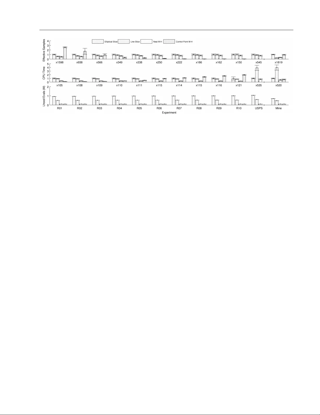
Elliptical slice sampling Iain Murra y Ry an Prescott Adams Da vid J.C. MacKa y Univ ersity of T oron to Univ ersity of T oron to Univ ersity of Cambridge Abstract Man y probabilistic models introduce strong dep endencies b etw een v ariables using a latent m ultiv ariate Gaussian distribution or a Gaus- sian pro cess. W e present a new Marko v c hain Mon te Carlo algorithm for p erforming infer- ence in mo dels with m ultiv ariate Gaussian priors. Its k ey prop erties are: 1) it has simple, generic co de applicable to many mo dels, 2) it has no free parameters, 3) it w orks w ell for a v ariety of Gaussian process based mo dels. These prop erties mak e our metho d ideal for use while mo del building, remo ving the need to sp end time deriving and tuning up dates for more complex algorithms. 1 In tro duction The m ultiv ariate Gaussian distribution is commonly used to sp ecify a priori b eliefs about dep endencies b et ween laten t v ariables in probabilistic mo dels. The parameters of suc h a Gaussian ma y be specified directly , as in graphical mo dels and Marko v random fields, or implicitly as the marginals of a Gaussian pro cess (GP). Gaussian pro cesses may be used to express concepts of spatial or temp oral coherence, or ma y more generally b e used to construct Bay esian kernel metho ds for non- parametric regression and classification. Rasm ussen and Williams (2006) pro vide a recent review of GPs. Inferences can only b e calculated in closed form for the simplest Gaussian laten t v ariable mo dels. Recen t w ork sho ws that posterior marginals can sometimes b e w ell approximated with deterministic metho ds (Kuss and Rasm ussen, 2005; Rue et al., 2009). Marko v chain Mon te Carlo (MCMC) metho ds represent joint p os- terior distributions with samples (e.g. Neal, 1993). MCMC can b e slo wer but applies more generally . App earing in Pro ceedings of the 13 th In ternational Con- ference on Artificial In telligence and Statistics (AIST A TS) 2010, Chia Laguna Resort, Sardinia, Italy . V olume 6 of JMLR: W&CP 6. Copyrigh t 2010 by the authors. In some circumstances MCMC pro vides goo d results with minimal mo del-sp ecific implementation. Gibbs sampling, in particular, is frequently used to sample from probabilistic mo dels in a straigh tforward wa y , up- dating one v ariable at a time. In mo dels with strong dep endencies among v ariables, including many with Gaussian priors, Gibbs sampling is kno wn to p erform p o orly . Several authors ha ve previously addressed the issue of sampling from mo dels con taining strongly cor- related Gaussians, notably the recen t work of Titsias et al. (2009). In this pap er we pro vide a technique called el liptic al slic e sampling that is simpler and of- ten faster than other metho ds, while also remo ving the need for preliminary tuning runs. Our metho d pro vides a drop-in replacement for MCMC samplers of Gaussian mo dels that are curren tly using Gibbs or Metrop olis– Hastings and we demonstrate empirical success against comp eting metho ds with several different GP-based lik eliho o d models. 2 Elliptical slice sampling Our ob jective is to sample from a p osterior distri- bution ov er latent v ariables that is prop ortional to the pro duct of a m ultiv ariate Gaussian prior and a lik eliho o d function that ties the latent v ariables to the observ ed data. W e will use f to indicate the vector of latent v ariables that w e wish to sample and denote a zero-mean Gaussian distribution with cov ariance Σ b y N ( f ; 0 , Σ) ≡ | 2 π Σ | − 1 / 2 exp  − 1 2 f > Σ − 1 f  . (1) W e also use f ∼ N (0 , Σ) to state that f is dra wn from a distribution with the densit y in (1) . Gaussians with non-zero means can simply be shifted to hav e zero-mean with a c hange of v ariables; an example will b e giv en in Section 3.3. W e use L ( f ) = p (data | f ) to denote the likelihoo d function so that our tar get distribution for the MCMC sampler is p ? ( f ) = 1 Z N ( f ; 0 , Σ) L ( f ) , (2) where Z is the normalization constant, or the marginal lik eliho o d, of the mo del. Our starting p oint is a Metrop olis–Hastings metho d in tro duced by Neal (1999). Giv en an initial state f , a Elliptical slice sampling new state f 0 = p 1 −  2 f +  ν , ν ∼ N (0 , Σ) (3) is prop osed, where  ∈ [ − 1 , 1] is a step-size parameter. The prop osal is a sample from the prior for  = 1 and more conserv ativ e for v alues closer to zero. The mov e is accepted with probabilit y p (accept) = min(1 , L ( f 0 ) /L ( f )) , (4) otherwise the next state in the chain is a copy of f . Neal reported that for some Gaussian process classifiers the Metropolis–Hastings metho d w as man y times faster than Gibbs sampling. The metho d is also simpler to implemen t and can immediately b e applied to a m uch wider v ariet y of mo dels with Gaussian priors. A drawbac k, identified b y Neal (1999), is that the step-size  needs to b e chosen appropriately for the Mark ov c hain to mix efficien tly . This may require preliminary runs. Usually parameters of the cov ariance Σ and likelihoo d function L are also inferred from data. Differen t step-size parameters may b e needed as the mo del parameters are up dated. It w ould b e desirable to automatically search ov er the step-size parameter, while maintaining a v alid algorithm. F or a fixed auxiliary random draw, ν , the lo cus of p ossible prop osals by v arying  ∈ [ − 1 , 1] in (3) is half of an ellipse. f 0 = ν sin θ + f cos θ , (5) defining a full ellipse passing through the curren t state f and the auxiliary draw ν . F or a fixed θ there is an equiv alent  that gives the same prop osal distribution in the original algorithm. Ho wev er, if we can searc h o ver the step-size, the full ellipse giv es a richer c hoice of up dates for a given ν . 2.1 Sampling an alternativ e mo del ‘Slice sampling’ (Neal, 2003) provides a wa y to sample along a line with an adaptive step-size. Proposals are dra wn from an interv al or ‘brack et’ which, if to o large, is shrunk automatically until an acceptable p oint is found. There are also wa ys to automatically enlarge small initial brack ets. Naively applying these adaptive algorithms to select the v alue of  in (3) or θ in (5) do es not result in a Mark ov chain transition op erator with the correct stationary distribution. The lo cus of states is defined using the current position f , which upsets the reversibilit y and correctness of the update. W e would like to construct a v alid Mark ov c hain tran- sition operator on the ellipse of states that uses slice sampling’s existing ability to adaptively pick step sizes. Input: curren t state f , a routine that samples from N (0 , Σ), log-likelihoo d function log L . Output: a new state f 0 . When f is drawn from p ? ( f ) ∝ N ( f ; 0 , Σ) L ( f ), the marginal distribution of f 0 is also p ? . 1. Sample from p ( ν 0 , ν 1 , θ | ( ν 0 sin θ + ν 1 cos θ = f ) ): θ ∼ Uniform[0 , 2 π ] ν ∼ N (0 , Σ) ν 0 ← f sin θ + ν cos θ ν 1 ← f cos θ − ν sin θ 2. Up date θ ∈ [0 , 2 π ] using slice sampling (Neal, 2003) on: p ? ( θ | ν 0 , ν 1 ) ∝ L ( ν 0 sin θ + ν 1 cos θ ) 3. return f 0 = ν 0 sin θ + ν 1 cos θ Figure 1: In tuition b ehind elliptical slice sampling. This is a v alid algorithm, but will b e adapted (Figure 2). W e will first in tuitively construct a v alid method by p ositing an augmented probabilistic mo del in which the step-size is a v ariable. Standard slice sampling algo- rithms then apply to that mo del. W e will then adjust the algorithm for our particular setting to pro vide a second, slightly tidier algorithm. Our augmented probabilistic mo del replaces the origi- nal latent v ariable with prior f ∼ N (0 , Σ) with ν 0 ∼ N (0 , Σ) ν 1 ∼ N (0 , Σ) θ ∼ Uniform[0 , 2 π ] f = ν 0 sin θ + ν 1 cos θ . (6) The marginal distribution ov er the original latent v ari- able f is still N (0 , Σ), so the distribution ov er data is iden tical. How ever, we can now sample from the p osterior ov er the new laten t v ariables: p ? ( ν 0 , ν 1 , θ ) ∝ N ( ν 0 ; 0 , Σ) N ( ν 1 ; 0 , Σ) L ( f ( ν 0 , ν 1 , θ ) ) , and use the v alues of f deterministically derived from these samples. Our first approac h applies t wo Monte Carlo transition op erators that leav e the new latent p osterior inv arian t. Op erator 1: join tly resample the latents ν 0 , ν 1 , θ giv en the constrain t that f ( ν 0 , ν 1 , θ ) is unchanged. Be- cause the effective v ariable of interest do esn’t change, the lik eliho o d do es not affect this conditional distribu- tion, so the up date is generic and easy to implement. Op erator 2: use a standard slice sampling algorithm to up date the step-size θ given the other v ariables. The resulting algorithm is giv en in Figure 1. The auxiliary mo del construction makes the link to slice sampling explicit, which makes it easy to understand the v alidity of the approach. How ever, the algorithm Murra y , Adams, MacKa y can b e neater and the [0 , 2 π ] range for slice sampling is unnatural on an ellipse. The algorithm that we will presen t in detail results from eliminating ν 0 and ν 1 and a differen t wa y of setting slice sampling’s initial prop osal range. The precise connection will b e giv en in Section 2.4. A more direct, technical pro of that the equilibrium distribution of the Marko v c hain is the target distribution is presen ted in Section 2.3. Elliptical slice sampling , our prop osed algorithm is giv en in Figure 2, which includes the details of the slice sampler. An example run is illustrated in Figure 3(a–d) . Ev en for high-dimensional problems, the states consid- ered within one up date lie in a tw o-dimensional plane. In high dimensions f and ν are likely to ha ve similar lengths and b e an angle of π / 2 apart. Therefore the ellipse will typically b e fairly close to a circle, although this is not required for the v alidity of the algorithm. As in tended, our slice sampling approac h selects a new lo cation on the randomly generated ellipse in (5) . There are no rejections: the new state f 0 is never equal to the current state f unless that is the only state on the ellipse with non-zero lik eliho od. The algorithm prop oses the angle θ from a brack et [ θ min , θ max ] whic h is shrunk exp onentially quick ly until an acceptable state is found. Thus the step size is effectively adapted on each iteration for the current ν and Σ. 2.2 Computational cost Dra wing ν costs O ( N 3 ), for N -dimensional f and gen- eral Σ. The usual implementation of a Gaussian sam- pler would inv olve caching a (Cholesky) decomp osition of Σ, suc h that draws on subsequent iterations cost O ( N 2 ). F or some problems with sp ecial structure dra w- ing samples from the Gaussian prior can be cheaper. In many mo dels the Gaussian prior distribution cap- tures dep endencies: the observ ations are indep endent conditioned on f . In these cases, computing L ( f ) will cost O ( N ) computation. As a result, drawing the ν random v ariate will b e the dominant cost of the up date in many high-dimensional problems. In these cases the extra cost of elliptical slice sampling ov er Neal’s Metrop olis–Hastings algorithm will b e small. As a minor p erformance improv emen t, our implementa- tion optionally accepts the log-likelihoo d of the initial state, if kno wn from a previous update, so that it do esn’t need to b e recomputed in step 2. 2.3 V alidit y Elliptical slice sampling considers settings of an angle v ariable, θ . Figure 2 presen ted the algorithm as it w ould be used: there is no need to index or remem b er the visited angles. F or the purp oses of analysis w e Input: curren t state f , a routine that samples from N (0 , Σ), log-likelihoo d function log L . Output: a new state f 0 . When f is drawn from p ? ( f ) ∝ N ( f ; 0 , Σ) L ( f ), the marginal distribution of f 0 is also p ? . 1. Choose ellipse: ν ∼ N (0 , Σ) 2. Log-lik eliho od threshold: u ∼ Uniform[0 , 1] log y ← log L ( f ) + log u 3. Dra w an initial prop osal, also defining a brack et: θ ∼ Uniform[0 , 2 π ] [ θ min , θ max ] ← [ θ − 2 π , θ ] 4. f 0 ← f cos θ + ν sin θ 5. if log L ( f 0 ) > log y then: 6. Accept: return f 0 7. else: Shrink the brack et and try a new p oint: 8. if θ < 0 then: θ min ← θ else: θ max ← θ 9. θ ∼ Uniform[ θ min , θ max ] 10. GoT o 4. Figure 2: The elliptical slice sampling algorithm. (a) (b) (c) (d) (e) Figure 3: (a) The algorithm receives f = as input. Step 1 dra ws auxiliary v ariate ν = , defining an ellipse cen tred at the origin ( ). Step 2: a likelihoo d threshold defines the ‘slice’ ( ). Step 3: an initial prop osal is drawn, in this case not on the slice. (b) The first prop osal defined b oth edges of the [ θ min , θ max ] brack et; the second prop osal ( ) is also drawn from the whole range. (c) One edge of the brac ket ( ) is mov ed to the last rejected p oint suc h that is still included. Prop osals are made with this shrinking rule until one lands on the slice. (d) The prop osal here ( ) is on the slice and is returned as f 0 . (e) Sho ws the reverse configuration discussed in Section 2.3: is the input f 0 , whic h with auxiliary ν 0 = defines the same ellipse. The brac kets and first three prop osals ( ) are the same. The final prop osal ( ) is accepted, a mov e back to f . Elliptical slice sampling will denote the ordered sequence of angles considered during the algorithm b y { θ k } with k = 1 ..K . W e first iden tify the join t distribution o ver a state dra wn from the target distribution (2) and the other random quantities generated by the algorithm: p ( f , y , ν , { θ k } ) = p ? ( f ) p ( y | f ) p ( ν ) p ( { θ k } | f , ν , y ) = 1 Z N ( f ; 0 , Σ) N ( ν ; 0 , Σ) p ( { θ k } | f , ν , y ) , (7) where the vertical level y w as dra wn uniformly in [0 , L ( f )], that is, p ( y | f ) = 1 /L ( f ). The final term, p ( { θ k } | f , ν , y ), is a distribution ov er a random-sized set of angles, defined by the stopping rule of the algorithm. Giv en the random v ariables in (7) the algorithm de- terministically computes p ositions, { f k } , accepting the first one that satisfies a likelihoo d constraint. More generally eac h angle specifies a rotation of the tw o a priori Gaussian v ariables: ν k = ν cos θ k − f sin θ k f k = ν sin θ k + f cos θ k , k = 1 ..K . (8) F or any c hoice of θ k this deterministic transformation has unit Jacobian. An y such rotation also leav es the join t prior probability inv arian t, N ( ν k ; 0 , Σ) N ( f k ; 0 , Σ) = N ( ν ; 0 , Σ) N ( f ; 0 , Σ) (9) for all k , whic h can easily b e v erified by substituting v alues in to the Gaussian form (1). It is often useful to consider how an MCMC algorithm could mak e a r everse tr ansition from the final state f 0 bac k to the initial state f . The final state f 0 = f K w as the result of a rotation b y θ K in (8) . Giv en an initial state of f 0 = f K , the algorithm could generate ν 0 = ν K in step 1. Then a rotation of − θ K w ould return back to the original ( f , ν ) pair. Moreov er, the same ellipse of states is accessible and rotations of θ k − θ K will repro duce any intermediate f k y ), ν 0 = ν K and angles, θ 0 k = ( θ k − θ K k < K − θ K k = K , (11) resulting in the original state f b eing returned. The rev erse configuration corresp onding to the result of a forw ards run in Figure 3(d) is illustrated in Figure 3(e) . Substituting (9) in to (7) sho ws that ensuring that the forw ard and reverse angles are equally probable, p ( { θ k } | f , ν , y ) = p ( { θ 0 k } | f 0 , ν 0 , y ) , (12) results in the rev ersible property (10). The algorithm do es satisfy (12) : The probability of the first angle is alw ays 1 / 2 π . If more angles w ere considered b efore an acceptable state was found, these angles w ere dra wn with probabilities 1 / ( θ max − θ min ). Whenever the brack et w as shrunk in step 8, the side to shrink m ust ha ve b een c hosen suc h that f K remained selectable as it w as selected later. The reverse transition uses the same in termediate prop osals, making the same rejections with the same likelihoo d threshold, y . Because the algorithm explicitly includes the initial state, whic h in rev erse is f K at θ 0 = 0, the reverse transition inv olves the same set of shrinking decisions as the forw ards transitions. As the same brac kets are sampled, the 1 / ( θ max − θ min ) probabilities for drawing angles are the same for the forw ards and reverse transitions. The reversibilit y of the transition op erator (10) implies that the target p osterior distribution (2) is a station- ary distribution of the Mark ov chain. Dra wing f from the stationary distribution and running the algorithm dra ws a sample from the joint auxiliary distribution (7) . The deterministic transformations in (8) and (11) ha ve unit Jacobian, so the probability density of obtaining a joint draw corresp onding to ( f 0 , y , ν 0 , { θ 0 k } ) is equal to the probabilit y given by (7) for the original v ari- ables. The reversible prop erty in (10) sho ws that this is the same probabilit y as generating the v ariables by first generating f 0 from the target distribution and gen- erating the remaining quantities using the algorithm. Therefore, the marginal probability of f 0 is giv en by the target p osterior (2). Giv en the first angle, the distribution ov er the first pro- p osed mo ve is N ( f cos θ , Σ sin 2 θ ). Therefore, there is a non-zero probabilit y of transitioning to any region that has non-zero probability under the p osterior. This is enough to ensure that, formally , the chain is irreducible and ap erio dic (Tierney , 1994). Therefore, the Marko v c hain has a unique stationary distribution and rep eated applications of elliptical slice sampling to an arbitrary starting p oint will asymptotically lead to p oints drawn from the target p osterior distribution (2). 2.4 Slice sampling v arian ts There is some amount of choice in ho w the slice sampler on the ellipse could b e set up. Other methods for prop osing angles could ha ve b een used, as long as they satisfied the reversible condition in (12) . The particular algorithm proposed in Figure 2 is app ealing because it is simple and has no free parameters. Murra y , Adams, MacKa y The algorithm must choose the initial edges of the brac ket [ θ min , θ max ] randomly . It w ould b e aesthet- ically pleasing to place the edges of the brack et at the opp osite side of the ellipse to the curren t position, at ± π . Ho wev er this deterministic brack et placemen t w ould not be reversible and gives an in v alid algorithm. The edge of a randomly-chosen brack et could lie on the ‘slice’, the acceptable region of states. Our recom- mended elliptical slice sampling algorithm, Figure 2, w ould accept this p oint. The initially-presen ted algo- rithm, Figure 1, effectively randomly places the end- p oin ts of the brack et but without chec king this lo cation for acceptabilit y . Apart from this small c hange, it can b e shown that the algorithms are equiv alent. In typical problems the slice will not co ver the whole ellipse. F or example, if f is a represen tative sample from a p osterior, often − f will not b e. Increasing the probabilit y of prop osing points close to the current state may increase efficiency . One wa y to do this would b e to shrink the brack et more aggressively (Skilling and MacKay, 2003). Another would b e to deriv e a mo del from the auxiliary v ariable mo del (6) , but with a non-uniform distribution on θ . Another wa y would b e to randomly p osition an initial brack et of width less than 2 π — the co de that we provide optionally allo ws this. How ever, as explained in section 2.2, for high- dimensional problems such tuning will often only give small improv ements. F or smaller problems we hav e seen it possible to improv e the cpu-time efficiency of the algorithm by around t w o times. Another p ossible line of research is metho ds for biasing prop osals aw a y from the curren t state. F or example the ‘ov er-relaxed’ metho ds discussed by Neal (2003) ha ve a bias tow ards the opp osite side of the slice from the current position. In our context it ma y b e desirable to encourage mov es close to θ = π / 2, as these mov es are indep enden t of the previous p osition. These prop osals are only likely to b e useful when the lik eliho o d terms are v ery w eak, ho wev er. In the limit of sampling from the prior due to a constant lik eliho o d, the algorithm already samples reasonably efficien tly . T o see this, consider the distribution ov er the outcome after N iterations initialized at f 0 : f N = f 0 N Y n =1 cos θ n + N X m =1 ν m sin θ m N Y n = m +1 cos θ n , where ν n and θ n are v alues drawn at iteration n . Only one angle is drawn p er iteration when sampling from the prior, b ecause the first prop osal is alw ays accepted. The only dep endence on the initial state is the first term, the co efficient of whic h shrinks tow ards zero exp onen tially quic kly . 2.5 Limitations A common modeling situation is that an unknown constan t offset, c ∼ N (0 , σ 2 m ) , has b een added to the en tire laten t vector f . The resulting v ariable, g = f + c , is still Gaussian distributed, with the constant σ 2 m added to ev ery elemen t of the cov ariance matrix. Neal (1999) iden tified that this sort of co v ariance will not tend to pro duce useful auxiliary draws ν . An iteration of the Mark ov chain can only add a nearly-constan t shift to the current state. Indeed, co v ariances with large constan t terms are generally problematic as they tend to b e p o orly conditioned. Instead, large offsets should b e mo deled and sampled as separate v ariables. No algorithm can sample effectively from arbitrary dis- tributions. As any distribution can b e factored as in (2) , there exist lik eliho o ds L ( f ) for which elliptical slice sampling is not effective. Man y Gaussian pro cess appli- cations hav e strong prior smoothness constraints and relativ ely w eak likelihoo d constraints. This imp ortant regime is where w e focus our empirical comparison. 3 Related w ork Elliptical slice sampling builds on a Metropolis– Hastings (M–H) up date prop osed b y Neal (1999). Neal rep orted that the original up date p erformed moderately b etter than using a more obvious M–H prop osal, f 0 = f +  ν , ν ∼ N (0 , Σ) , (13) and muc h b etter than Gibbs sampling for Gaussian pro cess classification. Neal also proposed using Hy- brid/Hamiltonian Mon te Carlo (Duane et al., 1987; Neal, 1993), which can b e v ery effective, but requires tuning and the implemen tation of gradients. W e now consider some other alternatives that ha v e similar re- quiremen ts to elliptical slice sampling. 3.1 ‘Con v en tional’ slice sampling Elliptical slice sampling builds on the family of methods in tro duced by Neal (2003). Several of the existing slice sampling metho ds would also b e easy to apply: they only require p oint-wise ev aluation of the posterior up to a constant. These metho ds do hav e step-size parameters, but unlik e simple Metropolis methods, t ypically the p erformance of slice samplers do es not crucially rely on carefully setting free parameters. The most popular generic slice samplers use simple univ ariate updates, although applying these directly to f w ould suffer the same slo w con v ergence problems as Gibbs sampling. While Agarw al and Gelfand (2005) ha ve applied slice sampling for sampling parameters in Gaussian spatial pro cess mo dels, they assumed a Elliptical slice sampling linear-Gaussian observ ation mo del. F or non-Gaussian data it was suggested that “there seems to b e little role for slice sampling.” Elliptical slice sampling changes all of the v ariables in f at once, although there are p otentially b etter wa ys of ac hieving this. An extensiv e search space of p ossibilities includes the suggestions for multiv ariate up dates made b y Neal (2003). One simple p ossible slice sampling up date performs a univ ariate up date along a random line traced out by v arying  in (13) . As the M–H method based on the line work ed less well than that based on an ellipse, one migh t also exp ect a line-based slice sampler to p erform less well. In tuitively , in high dimensions muc h of the mass of a Gaussian distribution is in a thin ellipsoidal shell. A straight line will more rapidly escap e this shell than an ellipse passing through tw o p oints within it. 3.2 Con trol v ariables Titsias et al. (2009) introduced a sampling metho d inspired b y sparse Gaussian process approximations. M con trol v ariables f c are introduced such that the join t prior p ( f , f c ) is Gaussian, and that f still has marginal prior N (0 , Σ). F or Gaussian pro c ess mo dels a parametric family of joint co v ariances was defined, and the mo del is optimized so that the control v ariables are informative about the original v ariables: p ( f | f c ) is made to b e highly p eaked. The optimization is a pre-pro cessing step that occurs b efore sampling b egins. The idea is that the small n um b er of control v ariables f c will b e less strongly coupled than the original v ariables, and so can be mov ed individually more easily than the comp onen ts of f . A prop osal inv olv es resampling one con trol v ariable from the conditional prior and then resampling f from p ( f | f c ). This mov e is accepted or rejected with the Metrop olis–Hastings rule. Although the metho d is inspired by an approximation used for large datasets, the accept/reject step uses the full mo del. After O ( N 3 ) pre-pro cessing it costs O ( N 2 ) to ev aluate a proposed c hange to the N -dimensional v ector f . One ‘iteration’ in the pap er consisted of an up date for eac h control v ariable and so costs O ( M N 2 ) — roughly M elliptical slice sampling up dates. The con trol metho d uses few er likelihoo d ev aluations p er iteration, although has some different minor costs asso- ciated with b o ok-keeping of the control v ariables. 3.3 Lo cal up dates In some applications it may make sense to up date only a subset of the latent v ariables at a time. This migh t help for computational reasons giv en the O ( N 2 ) scaling for dra wing samples of subsets of size N . Titsias et al. (2009) also identified suitable subsets for lo cal updates and then in vestigated sampling proposals from the conditional Gaussian prior. In fact, lo cal updates can b e combined with any tran- sition op erator for mo dels with Gaussian priors. If f A is a subset of v ariables to up date and f B are the remaining v ariables, we can write the prior as:  f A f B  ∼ N  0 ,  Σ A,A Σ A,B Σ B ,A Σ B ,B  (14) and the conditional prior is: p ( f A | f B ) = N ( f A ; m , S ) , where m = Σ A,B Σ − 1 B ,B f B , and S = Σ A,A − Σ A,B Σ − 1 B ,B Σ B ,A . A c hange of v ariables g = f A − m allo ws us to express the conditional posterior as: p ? ( g ) ∝ N ( g ; 0 , S ) L   g + m f B   . W e can then apply elliptical slice sampling, or any al- ternativ e, to up date g (and thus f A ). Updating groups of v ariables according to their conditional distributions is a standard wa y of sampling from a joint distribution. 4 Exp erimen ts W e p erformed an empirical comparison on three Gaus- sian pro cess based probabilistic mo deling tasks. Only a brief description of the mo dels and metho ds can b e given here. F ull co de to repro duce the results is pro vided as supplementary material. 4.1 Mo dels Eac h of the mo dels asso ciates a dimension of the latent v ariable, f n , with an ‘input’ or ‘feature’ vector x n . The mo dels in our exp eriments construct the cov ariance from the inputs using the most common method, Σ ij = σ 2 f exp  − 1 2 P D d =1 ( x d,i − x d,j ) 2 /` 2  , (15) the squared-exp onen tial or “Gaussian” co v ariance. This co v ariance has “lengthscale” parameter ` and an o verall “signal v ariance” σ 2 f . Other cov ariances ma y b e more appropriate in many mo deling situations, but our algorithm would apply unc hanged. Gaussian regression: giv en observ ations y of the laten t v ariables with Gaussian noise of v ariance σ 2 n , L r ( f ) = Q n N ( y n ; f n , σ 2 n ) , (16) the p osterior is Gaussian and so fully tractable. W e use this as a simple test that the method is working correctly . Differences in p erformance on this task will also give some indication of p erformance with a simple log-conca ve lik eliho o d function. Murra y , Adams, MacKa y W e generated ten synthetic datasets with input fea- ture dimensions from one to ten. Each dataset was of size N = 200 , with inputs { x n } N n =1 dra wn uniformly from a D -dimensional unit h yp ercub e and function v alues drawn from a Gaussian prior, f ∼ N (0 , Σ), using co v ariance (15) with lengthscale ` = 1 and unit signal v ariance, σ 2 f = 1. Noise with v ariance σ 2 n = 0 . 3 2 w as added to generate the observ ations. Gaussian pro cess classification: a well-explored application of Gaussian pro cesses with a non-Gaussian noise mo del is binary classification: L c ( f ) = Q n σ ( y n f n ) , (17) where y n ∈ {− 1 , +1 } are the lab el data and σ ( a ) is a sigmoidal function: 1 / (1 + e − a ) for the logistic classifier; a cumulativ e Gaussian for the probit classifier. W e ran tests on the USPS classification problem as set up by Kuss and Rasmussen (2005). W e used log σ f = 3 . 5 , log ` = 2 . 5 and the logistic likelihoo d. Log Gaussian Cox pro cess: an inhomogeneous P ois- son pro cess with a non-parametric rate can be con- structed by using a shifted dra w from a Gaussian pro- cess as the log-intensit y function. Approximate infer- ence can be p erformed by discretizing the space into bins and assuming that the log-in tensity is uniform in eac h bin (Møller et al., 1998). Eac h bin contributes a P oisson lik elihoo d: L p ( f ) = Y n λ n y n exp( − λ n ) y n ! , λ n = e f n + m , (18) where the mo del explains the y n coun ts in bin n as dra wn from a Poisson distribution with mean λ n . The offset to the log mean, m , is the mean log-intensit y of the Poisson pro cess plus the log of the bin size. W e p erform inference for a Cox pro cess model of the dates of mining disasters taken from a standard data set for testing p oint pro cesses (Jarrett, 1979). The 191 ev en ts w ere placed into 811 bins of 50 days each. The Gaussian pro cess parameters were fixed to σ 2 f = 1 and ` = 13516 days (a third of the range of the dataset). The offset m in (18) w as set to m = log(191 / 811) , to matc h the empirical mean rate. 4.2 Results A trace of the samples’ log-likelihoo ds, Figure 4, shows that elliptical slice sampling and control v ariables sam- pling ha v e differen t behavior. The metho ds make differ- en t types of mo v es and only con trol v ariables sampling con tains rejections. Using long runs of either metho d to estimate exp ectations under the target distribution is v alid. Ho w ever, stic king in a state due to many rejections can give a p o or estimator as can alwa ys mak- 0 500 1000 −45 −40 −35 # Control variable moves log L Control Variables 0 500 1000 −45 −40 −35 # Iterations Elliptical slice sampling Figure 4: T races of log-lik eliho o ds for the 1-dimensional GP regression experiment. Both lines are made with 333 p oints plotted after each sweep through M = 3 con trol v ariables and after every 3 iterations of elliptical slice sampling. 0 5000 10000 −140 −120 −100 −80 −60 −40 # Control variable moves log L Control Variables 0 5000 10000 −140 −120 −100 −80 −60 −40 # Iterations Elliptical slice sampling Figure 5: As in Figure 4 but for 10-dimensional regression and plotting ev ery M = 78 iterations. (Control v ariables didn’t mov e on this run.) ing small mov es. It can b e difficult to judge o verall sampling quality from trace plots alone. As a quantitativ e measure of qualit y w e estimated the “effectiv e num b er of samples” from log-likelihoo d traces using R-CODA (Cowles et al., 2006). Figure 6 shows these results along with computer time taken. The step size for Neal’s Metrop olis metho d w as chosen using a grid searc h to maximize p erformance. Times are for the pro vided implemen tations under Matlab v7.8 on a sin- gle 64 bit, 3 GHz Intel Xeon CPU. Comparing runtimes is alwa ys problematic, due to implementation-specific details. Our n umbers of effective samples are primarily plotted for the same num b er of O ( N 2 ) up dates with the understanding that some correction based lo osely on runtime should b e applied. The control v ariables approach was particularly recom- mended for Gaussian pro cesses with low-dimensional input spaces. On our particular low-dimensional syn thetic regression problems using control v ariables clearly outperforms all the other metho ds. On the mo del of mining disasters, con trol v ariable sampling has comparable p erformance to elliptical slice sampling with ab out 50% less run time. On higher-dimensional problems more con trol v ariables are required; then other methods cost less. Con trol v ariables failed to sam- ple in high-dimensions (Figure 5). On the USPS classifi- cation problem control v ariables ran exceedingly slowly and we were unable to obtain any meaningful results. Elliptical slice sampling obtained more effective samples than Neal’s M–H metho d with the b est p ossible step size , although at the cost of increased run time. On the problems inv olving real data, elliptical slice sampling Elliptical slice sampling Figure 6: Number of effective samples from 10 5 iterations after 10 4 burn in, with time and likelihoo d ev aluations required. The means and standard deviations for 100 runs are shown (divide the “error bars” by 10 to get standard errors on the mean, which are small). Each iteration inv olv es one O ( N 2 ) op eration (e.g. one ν dra w or up dating one control v ariable). Eac h group of bars in the top tw o rows has been rescaled for readability: the num b ers b eneath each group sho w the n umber of effective samples or CPU time in seconds for elliptical slice sampling, which alwa ys has bars of height 1. w as b etter ov erall whereas M–H has more effective samples p er unit time (in our implemen tation) on the syn thetic problems. The p erformance differences aren’t h uge; either metho d would w ork w ell enough. Elliptical slice sampling takes less time than slice sam- pling along a straigh t line (line sampling inv olves addi- tional prior ev aluations) and usually p erforms b etter. 5 Discussion The slice samplers use many more likelihoo d ev aluations than the other methods. This is partly b y c hoice: our co de can tak e a step-size parameter to reduce the n umber of likelihoo d ev aluations (Section 2.4). On these problems the time for lik eliho o d computations isn’t completely negligible: sp eedups of around × 2 ma y b e p ossible by tuning elliptical slice sampling. Our default p osition is that ease-of-use and human time is imp ortan t and that the adv antage of ha ving no free parameters should often b e taken in exchange for a factor of tw o in run time. W e fixed the parameters of Σ and L in our exp eri- men ts to simplify the comparison. Fixing the mo del p oten tially fav ors the metho ds that hav e adjustable parameters. In problems were Σ and L c hange dra- matically , a single step-size or optimized set of control v ariables could work very p o orly . Elliptical slice sampling is a simple generic algorithm with no t w eak parameters. It performs similarly to the b est p ossible p erformance of a related M–H scheme, and could b e applied to a wide v ariet y of applications in b oth low and high dimensions. Ac kno wledgemen ts Thanks to Michalis Titsias for co de, Sinead Williamson and Katherine Heller for a helpful discussion, and to Radford Neal, Sam Ro weis, Christophe Andrieu and the review ers for useful suggestions. RP A is funded by the Canadian Institute for Adv anced Research. References D. K. Agarw al and A. E. Gelfand. Slice sampling for sim ulation based fitting of spatial data mo dels. Statistics and Computing , 15(1):61–69, 2005. M. K. Cowles, N. Best, K. Vines, and M. Plummer. R- COD A 0.10-5, 2006. http://www- fis.iarc.fr/coda/ . S. Duane, A. D. Kennedy , B. J. Pendleton, and D. Ro w eth. Hybrid Monte Carlo. Physics L etters B , 195(2):216–222, Septem b er 1987. R. G. Jarrett. A note on the in terv als b etw een coal-mining disasters. Biometrika , 66(1):191–193, 1979. M. Kuss and C. E. Rasm ussen. Assessing appro ximate infer- ence for binary Gaussian pro cess classification. Journal of Machine L e arning R ese ar ch , 6:1679–1704, 2005. J. Møller, A. R. Syv ersveen, and R. P . W aagepetersen. Log Gaussian Cox pro cesses. Sc andinavian Journal of Statistics , 25(3):451–482, 1998. R. M. Neal. Probabilistic inference using Marko v chain Mon te Carlo metho ds. T ec hnical Rep ort CR G-TR-93-1, Dept. of Computer Science, Universit y of T oron to, 1993. R. M. Neal. Regression and classification using Gaussian pro cess priors. In J. M. Bernardo et al., editors, Bayesian Statistics 6 , pages 475–501. OU Press, 1999. R. M. Neal. Slice sampling. A nnals of Statistics , 31(3): 705–767, 2003. C. E. Rasmussen and C. K. I. Williams. Gaussian Pr o c esses for machine le arning . MIT Press, 2006. H. Rue, S. Martino, and N. Chopin. Appro ximate Bay esian inference for latent Gaussian mo dels by using integrated nested Laplace appro ximations. Journal of the Royal Statistic al So ciety: Series B , 71(2):319–392, 2009. J. Skilling and D. J. C. MacKay . Slice sampling — a binary implemen tation. Annals of Statistics , 31(3), 2003. L. Tierney . Mark ov chains for exploring p osterior distribu- tions. The Annals of Statistics , 22(4):1701–1728, 1994. M. Titsias, N. D. Lawrence, and M. Rattra y . Efficien t sampling for Gaussian pro cess inference using control v ariables. In A dvanc es in Neur al Information Pro c essing Systems 21 , pages 1681–1688, 2009.