Self-Calibration of Radio Astronomical Arrays With Non-Diagonal Noise Covariance Matrix

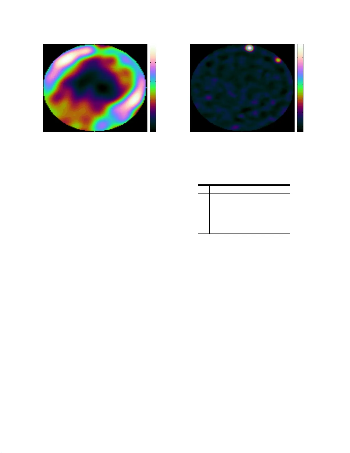
SELF-CALIBRA TION OF RADIO ASTRONOMICAL ARRA YS WITH NON-DIAGONAL NOISE CO V ARIANC E MA TRI X Stefan J. Wijnholds and Al le- Jan van der V e en ASTR ON R&D Department Oude Hoo g eveensedijk 4, NL-7991 PD, Dwingelo o, The Nether la nds phone: +31 521 595 2 6 1, email: wijnholds@astro n.nl web: www.astro n.nl Delft Universit y o f T echnology Department of Electr ical Eng ineering Mekelw eg 4 , NL-2 628 CD, Delft, The Netherla nds phone: +31 15 278 6240, e mail: allejan@cas .e t.tudelft.nl web: www.tudelft.nl ABSTRA CT The radio astronomy communit y is c ur rently building a nu mber of phased array telescop e s. The c alibration of these telescop es is hamp e r ed by th e fact that co v ariances of signals fro m clo sely s paced antennas are s e ns itive to noise coupling and to v ar iations in sky bright nes s on large spatial scales. These effects are difficult and com- putationally exp ensive to model. W e pr op ose to model them phenomenologically us ing a non- diagonal noise co- v ariance ma tr ix. The parameters can b e estimated us- ing a weigh ted a lter nating le a st squares (W ALS) a lgo- rithm iter ating betw een the calibration pa rameters and the a dditive nuisance pa r ameters. W e demonstra te the effectiveness of o ur metho d using data fro m the low fre- quency array (LO F AR) proto t yp e station. 1. INTR ODUCTION The radio astronomical communit y is currently con- structing a num b er of lar ge scale phased arr ay telescop es such as the low-frequency array (LOF AR) [1] and the Murchison wide field array (MW A) [2]. These ins tru- men ts ne e d to b e ca librated regular ly to track v aria- tions in the ele c tronics of the a ntennas and receivers, as well as direction dep endent v ariations of the iono- sphere [3]. E .g., LOF AR will consist of order 50 sta- tions (distributed o ver an area of a hundred kilo me- ters o r more), where each statio n consis ts of 96 “ low band” dual- p o larized dip ole antennas (10–90 MHz) and 96 “high band” antennas (11 0–24 0 MHz). The latter antennas are in turn comp osed of 1 6 b eamfor med dual- po larized dro o py dip ole antennas. Each station pro vides a num b er of b eamformed outputs, whic h in turn are cor - related a t a central lo cation to for m image s and other astronomy pr o ducts. In this pap er we fo cus o n the calibration of the sta- tion antennas. The genera l a im is to estimate the direc- tion independent ga ins and phases o f each sensor, as well as the dire c tion dep endent gains cor resp onding to each source. This is done for the 2–1 0 brightest s ources in the s k y , assuming a p oint sour ce mo del. The pr oblem is complicated by the fact that the cov ariances of s ig- nals fro m c lo sely s paced a nt enna s within a s tation are sensitive to noise coupling (for the low est frequencies, This work was supp orted by the Netherlands Institute for Radio Astronom y (ASTRON) and by NW O-STW under the VICI programme (DTC.5893). the antennas a r e spac ed closer than half a w avelength). Also, the p oint s ource mo del do es not entirely ho ld be - cause of bright emiss ion from the plane of the ga laxy , extending ov er the entire sky . F ortunately , this emissio n is spatially smooth, which implies that it is dominant on the short spa tial scales in the ar r ay ap ertur e , i.e. on the short ba selines. In this pap er we prop ose to mo del b oth short baseline effects by an additive noise cov a riance ma- trix, which in this case is not diagonal and has unkno wn ent r ies for each short baseline. If we can estima te this matrix, a simple p oint so urce mo del will b e sufficien t to calibrate the a rray , whic h r e duce s the problem to a problem for whic h so lutions are rea dily av aila ble [4–6]. Direction finding problems for ca librated arrays in the presence o f unknown correlated noise have been extensively studied in the 1990s. It was proven that the general pr oblem is not tractable without imp osing some appropriate constraints on the noise cov a riance matrix or explo iting differences in temp oral character- istics b etw een s o urce and no ise sig na ls [7]. Radio as tro- nomical sig nals gener ally b ehav e like noise, th us temp o- ral techniques (instrumental v ariables) are no t applica- ble. Instea d, we should rely on an appropria tely con- strained parameterized mo del of the no ise cov ariance matrix. Starting with [8], a s eries of pap er s were pub- lished; see [9] for an ov erv iew. ML estimators for the source and instrument par ameters under a generaliz ed noise cov ariance pa rameteriza tion is provided in [9, 10], whereas no nlinear leas t squares estimator s were stud- ied in [10–12]. In either case , an analytic sour ce a nd instrument para meter dep endent so lution is der ived fo r the noise mo del para meters which is subs tituted back int o the cost function. This co st function then has to b e minimized using a g eneralized solving technique, such as Newton itera tions. This approach works w ell if the nu mber o f instrumen t a nd source parameters is small. F or larg e r pro blems (w e consider 100 antenna/source pa- rameters and ov er 750 noise cov ariance parameters ), it is c o nv enient to explo it sub o ptimal but clos ed-form a n- alytic solutions, a t least for initializatio n. W e therefore prop ose a weigh ted alternating least squares (W ALS) approach which iterates ov er noise, source and instr u- men t parameters. The pro p osed metho d can th us be regar ded as an extension to the metho ds pr op osed in [6] Notation : The transp os e op e r ator is deno ted by T , the complex conjugate (Hermitian) tr ansp ose by H , complex conjuga tion by ( · ) a nd the pseudo-inv er se by † . An es timated v alue is deno ted by c ( · ). ⊗ denotes the Kronecker pro duct a nd ◦ is use d to denote the Kha tri- Rao o r column-wise Kr oneck er pro duct of tw o matr i- ces. vec( · ) conv er ts a matr ix to a vector by stacking the columns of the matrix . 2. D A T A MODEL AND PROBLEM ST A TEMENT W e consider an array of P ant enna s . The measured P × P array cov ariance matrix can be mo deled a s R = R 0 ( θ ) + Σ n (1) where R 0 ( θ ) is the signal mo del for an ideal nois e free array , which dep ends o n a num b er o f unknown r eal v al- ued pa r ameters accumulated in a column vector θ , and Σ n is a P × P matrix describing the no ise corr uptio n. Note that Σ n m ust b e Hermitian, since the array cov a ri- ance matr ix is a Hermitian matrix. In o ur applica tion, the data cov ar iance mo del is R 0 ( θ ) = G 1 A G 2 Σ s G H 2 A H G H 1 (2) where Σ s is the cov ariance o f the p oint sources (assumed to b e known from tables), A contains the direction vectors, G 1 a (diago na l) instrument a l gain/pha se ma- trix, and G 2 a (diago nal) directio n dep endent gain ma- trix [6]. If the dir ection dependent gains a r e unknown, we can introduce Σ = G 2 Σ s G H 2 , which implies that w e should estimate the apparent source p ow ers. The dir ec- tion dependent gains fo llow directly from the appare nt source p ow ers if the a ctual s ource p ow ers a re known, e.g. from ta ble s . If the source p ositio ns a re unknown or p erturb ed b y propagatio n conditions, A may b e pa- rameterized [6]. The con tents of the parameter vector θ therefor e strongly de p end o n the av aila ble knowledge on the instrument, the propaga tion conditio ns and the sources. As in [8] and subsequent pap ers, the unknown noise cov a riance matrix is mo deled a s a linear sum of known matrices, in this case simple selection matrices E ij which are ze r o everywhere ex cept for a ’1 ’ in e ntry ( i, j ), Σ n = X ( i,j ) ∈S σ ij E ij . The set S con tains the index pa irs of the s hort base- lines, including the auto co rrelation entries ( i, i ). The unknown co efficients σ ij are the n uisa nce parameters. In the absence of the no ise co rruptions, i.e., R = R 0 ( θ ), the estimation pr oblem to find the par ameter vector θ is commonly formulated either as a ML prob- lem, o r as a generalized least squar es estimation problem b θ = argmin θ w w w W  b R − R 0 ( θ )  W w w w 2 F , (3) where b R is the measured a rray cov ariance ma trix. It is known that with W = R − 1 / 2 this estimator is asymp- totically unbiased and asymptotically efficient [10, 12]. Indeed, the simulations in [10] show only a small im- prov ement of the ML solution as compared to the WLS solution. F or R 0 ( θ ) given in (2), this problem, a s w ell as the case with an unknown diagonal no is e cov ariance, was studied b y us in [6], in the pr e s ent pap er, we will assume that a solution to this pr oblem is av ailable. In the presence of correla ted noise on the short base- lines, the problem is e x tended to n b θ , b σ n o = argmin θ , σ n w w w W  b R − R 0 ( θ ) − Σ n  W w w w 2 F , (4) where σ n is a vector co ntaining all unique real v alued parameters required to describ e the nonzero en tries of Σ n . This vector can b e related to Σ n using a s election matrix I s such that v ec ( Σ n ) = I s σ n . By choos ing the selection matrix appropriately , we can ensure that the estimated Σ n is Her mitian. 3. P ARAMETER E STIMA TION 3.1 W ei gh ted Alternating Least Squares W e pro p ose to s olve the pr o blem in E q. (4) by alternat- ing b etw een weighted least squares (WLS) estimation of the desired parameters θ and WLS estimation of the nu isa nce parameters σ n . The firs t WLS problem can be formulated as b θ = argmin θ w w w W  b R − Σ n  − R 0 ( θ )  W w w w 2 F . (5) which is ident ica l in form to Eq. (3) for which a solution is assumed to be av ailable. The s e cond WLS pr oblem can b e form ulated as b σ n = argmin σ n w w w W  b R − R 0 ( θ )  − Σ n  W w w w 2 F = argmin σ n w w w  W ⊗ W  vec  b R − R 0 ( θ )  −  W ⊗ W  I s σ n w w w 2 F . (6) The solution to this pr oblem is given by b σ n =  W ⊗ W  I s  †  W ⊗ W  vec  b R − R 0 ( θ )  . (7) In se c tio n 2 it was mentioned that W = R − 1 / 2 pro- vides optimal weigh ting for the LS co st function. Since R is not known, b R is used instead in many applica tions. It ca n b e shown that this ma y lead to a bias in the es- timate of b σ n for a finite num ber of samples [6]. This bias can be av oided b y using the best av ailable mo del R  b θ , b σ n  instead of b R . Estimation of receiver no ise powers is a sp ecial case of the gener a l problem treated here. In this case Σ n is a diagonal, a nd I s = I ◦ I wher e I is the P × P identit y matrix. This form of selection matrix simplifies Eq. (7) considerably [6]. In s ome problems, for example in es- timating the receiver based gains, it is then p ossible to simply ignore the diagona l entries instead of including nu isa nce parameters [5]. It can fur ther b e shown that ignoring the co r rupted entries instead of including them using nuisance parameters do es no t change the Cram` er- Rao b ound o f the parameters of interest [13]. This can be explained intuitiv ely b y regarding the matrix equa- tion des cribing the WLS problem as a set of scala r equa - tions. If a unique nuisance parameter is added to one o f those scalar equatio ns, that e q uation is r equired to s o lve for the nuisance parameter and can thus not b e used to solve any other parameters . T his implies that this equa- tion could hav e b een igno r ed if one would only fo cus on the parameter s of in teres t. In practice, ho wever, it may be hard to develop an algorithm that ignores the cor- rupted e ntries in a sta tistically efficient wa y . 3.2 Algorithm The r esulting algorithm is as fo llows: 1. Initialization Se t the iteratio n counter i = 1 and ini- tialize b σ [0] n based on a ny prior information if av ail- able, o therwise initialize b σ [0] n to zer o. Initially use W = b R − 1 / 2 . 2. Estimate b θ [ i ] by solving the WLS problem fo r mu- lated in Eq. (5) using b σ [ i − 1] n as prior k nowledge. 3. Estimate b σ [ i ] n using Eq . (7) using b θ [ i ] as prior k nowl- edge. 4. Up date W = R − 1 / 2 to a void the bias mentioned in the previous section. 5. Che ck for c onver genc e , otherwise co ntin ue with step 2. An algorithm that alternatingly optimizes for dis- tinct gr oups o f para meters, in our case θ and σ n , can be prov en to conv er ge if the v a lue of the cost function decreases in each iteration. W e assume that a suitable metho d is av aila ble to find θ . Since w e propo se to es- timate σ n using the well kno wn standar d solution for least squa res es timation problems, the v alue of the cost function will decrea se in both steps, th us ensuring con- vergence. Although there is no guarantee that the al- gorithm w ill c o nv erge to the global o ptimu m, practical exp erience with LOF AR a nd r esults from Monte Carlo simulations in this pap er and in ea rlier pap ers [5, 6] in- dicate that the prop osed metho d pro duces go o d re s ults for most r easonable initial e s timates. 4. EXPERIME NT AL RESUL TS 4.1 The LOF AR protot yp e station The fir st full-scale LOF AR proto t yp e station with rea l- time back end beca me op eratio nal in the second qua r- ter of 2006 [14]. This sta tion consisted of 48 dual- po larizatio n antenn a s op erating b etw een 10 and 90 MHz arrang ed in a randomize d configuratio n based on rings with ex p o nentially increasing ra dii as shown in Fig. 1. Each of the tw o signa ls fr om ev er y antenna was filtered and digitized using a 12-bit 200 MHz ADC. A real- time FPGA based digital pro cessing back end splits the 100 MHz Nyquis t sa mpled base band in 512 subbands, each 195 k Hz wide, using a po lyphase filter. The backend also pr ovides a cor relator which can correla te in r eal- time the data fro m the 9 6 input channels for a single subband. This s ubband may be any of the 512 av ailable subbands and this choice ma y change every se cond. −30 −20 −10 0 10 20 30 −30 −20 −10 0 10 20 30 West ← x → East South ← y → North Figure 1: Array config uration o f the 48 an tenna LOF AR prototype station. West ← l → East South ← m → North −1 −0.5 0 0.5 1 −1 −0.8 −0.6 −0.4 −0.2 0 0.2 0.4 0.6 0.8 1 0.65 0.7 0.75 0.8 0.85 0.9 0.95 1 Figure 2 : Calibrated all-s k y map for a single pola riza- tion at 50 MHz fr o m the 4 8-element LOF AR pro totype station. The imag e s hows the sky pro jected on the hori- zon plane of the sta tion. 4.2 Res ults F or the demonstr ation in this paper w e used data from a single 1 s s napshot o bserv ation in the 195 kHz subband centered a t 50 MHz. This o bserv ation was done on 14 F ebruar y 2 008 at 1:42:0 7 UTC. W e will c alibrate the data using the metho d describ ed in Sec. 3.2, wher e we will mo del correla ted noise terms on all baselines shorter than four w av elengths. The co mplete WLS problem th us implies estimation of the amplitudes (48 para m- eters) and phases (47 pa rameters) of the antenna based complex g ains, the source p ow er ra tio of the tw o bright- est sources (1 parameter) a nd 7 64 rea l v alued n uisa nce parameters describing all non- zero ent r ies of the noise cov a riance matrix for a total of 860 fr ee r eal v alued pa- rameters p er p olar ization. In this exp eriment we show that use of such n uisa nce parameter s can re duce the complex so urce s tructure o n the sky to a simple mo del with just t wo p oint s ources. West ← l → East South ← m → North −1 −0.5 0 0.5 1 −1 −0.8 −0.6 −0.4 −0.2 0 0.2 0.4 0.6 0.8 1 0.65 0.7 0.75 0.8 Figure 3: Ca librated all-s ky map of ex tended emission observed at bas elines shorter than four wa velengths for a single p o larization at 5 0 MHz. Figure 2 shows a ca librated all sky map fo r a sin- gle p ola rization. There are t wo bright p oint sources near the nor theastern ho rizon. The image als o shows a lot of extended emissio n from the ga lactic plane (on the northw ester n hor izon) and the north p olar s pur (on the easter n horizon). T his extended emiss ion is hard to mo del accur ately , but only affects the short ba selines since short distances in the ap ertur e plane of a phased array cor resp ond to low spatial frequencies, which de- scrib e the structure on la rge s patial scales. It was found that most o f this extended emis s ion is captured b y the corre la tions o n baselines shorter tha n four wav elengths. This a ffects 3 58 cro s scorr e lations and the 48 auto cor relations resulting in the aforementioned 764 rea l v alued parameter s to describ e the non- zero en- tries of Σ n . Using the pro cedure outlined in the pre- vious s ection, b σ n was estimated simultaneously with b θ containing the other parameters. b Σ n can therefore be int er preted as an estimate of the e x tended source struc- ture, noise coupling and r eceiver noise p ow ers. This is nicely demons trated in Fig. 3 which shows an imag e based on b Σ n after the calibration was completed. Figure 4 shows the differ e nc e betw een the maps shown in Figs. 2 and 3. This shows that Σ n provides a description of the extended emissio n that is sufficien tly accurate to reduce b R − b Σ n to an array cov ariance matrix that ca n be des c rib ed by a mo del co nsisting of only tw o po int sour ces. T his thus reduces our original problem to one that has been discussed extensively in the ar r ay signal pr o cessing literature. 5. IMPR OVING THE COMPUT A TIONAL EFFICIENCY The ca lculation o f b σ n using Eq. 7 forms the most expen- sive part of the algo rithm in terms of CPU and memor y usage due to the K roneck er pr o ducts. These Kronecker pro ducts can only b e reduced to simpler K hatri-Rao o r Hadamard pro ducts in a num b er of special cas e s , such as a diagonal noise cov ariance matrix treated in [6]. Ho w- West ← l → East South ← m → North −1 −0.5 0 0.5 1 −1 −0.8 −0.6 −0.4 −0.2 0 0.2 0.4 0.6 0.8 1 0 0.05 0.1 0.15 0.2 0.25 Figure 4: Difference b etw een the calibr ated all- sky ma p shown in Fig. 2 a nd the contribution of extended emis- sion shown in Fig. 3 showing that the re mainder can b e accurately modeled using a model with just t wo p oint sources. # l m σ 2 q 1 0.2465 1 -0.716 37 1.0 0000 2 -0.343 46 0.7688 3 0.88 051 3 -0.131 25 -0.31 463 0 .79079 4 -0.299 41 -0.52 339 0 .74654 5 0.3929 0 0.5890 2 0.69781 T able 1: Source p owers and source lo catio ns used in the simulations ever, the par ameterization of Σ n chosen here implies that ea ch en try o f the ar ray cov ariance ma trix with a contribution from Σ n is a ffected by a unique additive parameter. Intuitiv ely , o ne w ould therefore exp ect that the weight ing in E q. (7) would not make m uch differ- ence. Omitting this would reduce the CPU and memo r y requirements considerably , since the Kroneck er pro ducts and the inverse increas e the numerical complexity from o  N P 2  to o  N 3 + P 6  and the size of the la rgest ma- trix from P 2 × N to P 2 × P 2 , where N is the num b er of noise parameters stack ed in σ n . This idea was therefore tested in Mo nte Carlo sim- ulations. F or these s imulations, a five armed arr ay w a s defined, each ar m b eing an eight-elemen t, one w av e- length spaced ULA. The fir st element o f each a rm formed an equa lly spaced cir cular array with ha lf wa ve- length spacing b etw een the elements. The source mo del is presen ted in T able 1. This sour ce mo del w as g ener- ated with a ra ndom n umber gener ator to verify that the prop osed approa ch works for arbitrar y so ur ce mo dels. Figure 5 compar es the v ariance o n the estimates for the omnidirectiona l complex gains of the receiv ing ele- men ts and the source powers obtaine d a fter 100 runs of a Monte Carlo simulation with weighted LS estimation of b σ n and the co mputationally mo re efficient unw eig hted LS estimation of b σ n . The complex receiving elemen t gains and the source p owers, stac ked in θ , were esti- 0 20 40 60 80 100 1 2 3 4 5 6 7 8 9 10 x 10 −4 parameter index variance WLS Σ n estimate LS Σ n estimate Figure 5: Co mparison of the v ariance on the direc- tion indep endent complex gain and the so urce p ower estimates obtained in Monte Carlo simulations with weigh ted LS es timation of b σ n and unw eighted LS es- timation o f b σ n . mated using w eighted least squar es in both cases. Both algorithms generally conv erg e d within three iterations to r elative err o r p er para meter of ∼ 10 − 4 , i.e. w ell below the Cr am` er-Rao b ound. The conv erg ence rate in these simulations was one digit p er iteration down to the nu- merical accur acy provided by double precision floating po int num b ers . The results indicate that the v ariance on these esti- mates is the same in both ca ses within the a ccuracy provided b y the sim ulatio ns. W e therefor e conclude that it is viable to discard the weight ing in Eq. (7). With this mo difica tion a ll 86 0 free parameters in the exp eriment describe d in the previous se c tion could b e extracted fro m the a ctual da ta using Matla b running on a standard dual core 2.4 GHz CPU in only 0.4 sec- onds. This implies that a sing le 2.4 GHz core can keep up with the data from the correlator at the LOF AR station, which r eal-time corr elates the antenna signals for a single s ubba nd with o ne second integration time. This update rate is required to track v ariations in the electronic g ains and the io nosphere. 6. CONCLUSIONS W e ha ve demonstrated using data from a LOF AR pro to- t yp e station that the effects of noise coupling , receiver noise powers and ex tended emission on a radio astro- nomical phased array can be phenomenologically de- scrib ed by a non-dia gonal noise cov a riance matrix with non-zero entries on short baselines. These en tries can b e computationally efficient and accurately estimated by a W ALS alg orithm alternating b etw een estimation o f the correla ted no ise par ameters and calibra tio n parameters. REFERENC ES [1] M. de. V os, A. W. Gunst and R. Nijbo er , “The LOF AR T elescop e: System Architecture and Sig nal Pro cess ing,” IEEE Pr o c e e dings , 2009, accepted for publication. [2] C. Lonsdale, “ The Murchison Widefield Array,” in Pr o c e e d ings of the XXIXth Gener al A ssembly of t he International U nion of R adio Scienc e (URSI GA) , Chicago (Ill.), USA, 7-16 Aug . 200 8. [3] S. v an der T ol, B. Jeffs and A. J. v an der V een, “Self Calibra tion for the LOF AR Radio Astronom- ical Array ,” IEEE T r ans. Signal Pr o c essing , vol. 55, no. 9 , pp. 4 497– 4510, Sept. 2007 . [4] D. R. F uhr mann, “E stimation of Sensor Gain a nd Phase,” IEEE T r ans. Signal Pr o c ess ing , v o l. 42, no. 1, pp. 7 7–87 , Jan. 1994. [5] S. J. Wijnholds and A. J. Bo onstra , “A Multi- source Calibration Method for Phase d Array Radio T elesco pe s ,” in F ourth IEEE Workshop on S en- sor A rr ay a n d M ult i-channel Pr o c ess ing (SAM) , W altham (MA), 12-1 4 July 200 6. [6] S. J . Wijnholds and A. J. v an der V een, “Multi- source Self-Calibration for Sensor Arr ays,” IEEE T r ans. Signal Pr o c essing , 20 09, in press. [7] P . Stoica and T. S¨ oderstr¨ om, “On Array Signal Pro cess ing in Spatially Co rrelated Noise Fields,” IEEE T r ans. Cir cuits and Syst ems - II: Analo g and Digital Signal Pr o c essing , v ol. 39, no . 12, pp. 879 – 882, Dec. 1 992. [8] J. F. Bohme and D. Kr aus, “On Least Squares Metho ds for Direction of Ar riv al Estimatio n in the Presence of Unknown Nois e Fields,” in IEEE Inter- national Confer enc e on Ac oust ics, Sp e e ch and Sig- nal Pr o c essing (ICASSP) , 1988, pp. 28 33–2 836. [9] B. G¨ oransson and B. Ottersten, “Direction E s ti- mation in Partially Unknown Noise Fields,” IEEE T r ans. Signal Pr o c essing , vol. 47 , no. 9, pp. 2375– 2385, Sept. 1999. [10] B. F riedlander and A. J. W eiss, “Direction Finding Using Noise Cov ar iance Mo deling ,” IEEE T ra ns. Signal Pr o c essing , vol. 43, no. 7, pp. 155 7–15 67, July 1995. [11] M. W a x, J, Sheinv ald a nd A. J. W eiss, “Detection and Loca lization in Color ed Noise via Generalized Least Squar e s ,” IEEE T r a ns. Signal Pr o c essing , vol. 44, no. 7, pp. 1 734– 1 743, J uly 1996. [12] B. O tter sten, P . Stoica and R. Ro y, “Cov ariance Matsching E stimation T ec hniques fo r Array Signal Pro cess ing Applications,” Digital Signal Pr o c ess- ing, A R eview J ournal , vol. 8, pp. 185 –210 , J uly 1998. [13] S. v an der T ol and S. J. Wijnholds, “CRB Anal- ysis o f the Impact of Unkno wn Receiver Noise o n Phased Array Calibration,” in F o u rth IEEE Work- shop on Sensor A rr ay and Multi-cha nn el Pr o c essing (SAM) , W altham (MA), 12- 14 July 2006 . [14] A. W. Gunst and M. J. Bentum, “The C ur rent Design o f the LOF AR Instrument,” in Pr o c e e d- ings of the 2007 IEEE International Confer enc e on S ignal Pr o c essing and Communic ations (ICSPC 2007) , Dubai, United Arab E mirates, 24-27 Nov. 2007.