Structure-Aware Stochastic Control for Transmission Scheduling

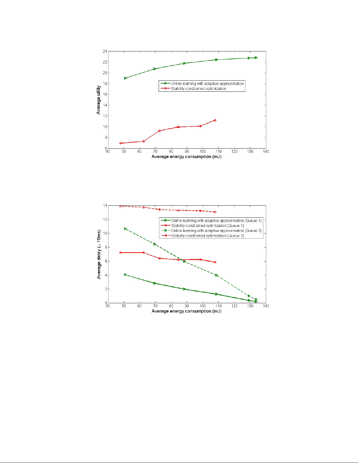
1 Structure-Aw are Stochastic Contro l for Transmission Scheduling Fa ng we n F u a nd Mih ae la va n d er Sch aa r Department of Electrical Engineering, Univ ersity of California, Los Angeles, Los Angeles, CA, 90095 {fw fu, mihaela}@ee.ucla.edu ABSTRACT In this paper, we consi der the problem of rea l- time t ransmission sch eduling over time-v arying channels. We first formulate the transmission scheduli ng problem as a Markov decis ion proce ss (MDP) and systematically unravel the struct ural pr operties (e.g. concavity in the st ate-v alue function and monotonicit y in the opt imal scheduling poli cy) exhibit ed by the opti m al solut ions. W e then pr opose an onl ine l earning al gorithm whic h preserves these s tructural prope rties and achieves ε -optimal s olutions for an arbi trarily small ε . The advantages of the propo sed online method are tha t: (i) it does not require a priori knowledge of t he traff ic arrival and channel statis tics and (ii) it adap tively a pproximates the s tate-v alue functions using piece-wise li near functi ons and has low stora g e and computation complexity. We also exten d the proposed low-com plexit y onl ine lea rning soluti on to the prioriti zed data transmission. The simulation result s dem onstrate t hat the proposed m ethod achieves significant ly better utili ty (or delay)-energy trade-offs when co m paring to exis ting state-of-art onli ne optimization methods. Keyw ords : Energy -efficient data transmission, Delay- sensitive comm unications, Markov decision processes, stochast ic control, sche duling I. INTRODUCTION Wirele ss systems often opera te in dynam ic environments where they experience t ime- varying channel condi tions (e.g. fading c hannel) and dy namic traff ic arri v als. To i m prove the energy effi ciency of s uch s ystem s while meeting the delay requirements of the suppo rted applic ations, the scheduling de cisions (i .e. determining how much data s hould be transmitted at e ach ti m e) should be ada pted to the time-v arying environ m ent [1][9]. In other words, it i s essential t o design scheduli ng policies which conside r the t ime- varying characteri stics of the chann els 2 as well as that of the a pplications (e.g. backlog in the transmission buffer, prioriti es of traf fic, e tc.). I n t his pa per, we us e opti m al stochasti c contr ol to deter m ine the transmission scheduling policy that maximizes the application utilit y g iven energy constraints . The problem of e nergy -efficient scheduling for t ransmission over wi reless chan nels has been intensi vely investigated in [1]-[15]. In [1] , the trade-off between t he average delay and the average ene rgy consumption for a fading cha nnel is charact erized. T he optimal energy consumption i n the asymptotic lar ge d elay region ( which corresponds to the cas e where the optimal energy cons um ption is cl ose to the optimal energy co nsum ption under queue st ability cons traints, as shown in Figure 1) i s anal y zed. I n [8], j oint source-channel coding is consi dered t o improve the delay-energy trade-off. The str uctural propert ies of the soluti ons which achie ve the opti m al ener gy - delay tra de- off are provided in [5][6 ][7]. I t is pr oven that the optimal am ount of data t o be transmission increa ses as th e backlog (i.e. buffer occupanc y ) increase s, and dec reases as the channel c onditions degrade. It is also proven that the optimal stat e- value function ( representing the optimal long-term ut ility starting from one st ate) is concave in terms of the instantaneous ba cklog . Energy- effici ent scheduli ng for traffi c with individual delay deadline s is conside red in [2] [3][4]. In [2], the optimal scheduling polic y is obtained using dynamic programm ing. In [3][4] , optimality condi tions ar e characte rized for the optimal sch eduling polici es, and based on t hese, onl ine heuristi c sche duling pol icies are developed. Besides considering t he time-varying channel conditions, the heterogeneous tr affic feature s (e.g. differe nt delay dea dlines, importanc e and dependencies of packets) are considered in [14][15], where the optimal scheduling poli cies are developed by expli citly considerin g the impact of the heterogeneous data traffic. We notice that the above solut ions are chara cterized by assuming that the statis tical knowledge of the underlying dynamics (e.g. channel stat e dis tribution, packet ar rival dis tribution, et c.) is known. When t he knowledge is una v ailabl e, only heuri stic solu tions are pr ovided, which cannot guarantee th e optimal performance. In order to cope wit h t he unknown environment, the stab ility-constrained optimization methods are developed in [ 10]-[13], where, instea d of minimizing the q ueue dela y , the queue s tability is considere d. The optimal energy consumption is achi eved only fo r as y mptoticall y large queue si zes (cor responding to asym ptotic 3 large d elays, i.e. in lar g e del ay region). T hese methods do not pr ov ide op timal ene rgy consumption in the small delay region which is s hown in Figure 1. Figure 1. Illustration of large d elay region and sm all delay region Other methods for copi ng with trans m ission i n unknown environment r ely on online lear ning algorithms developed based on reinforc em ent learni ng for Markov deci sion proc esses i n which the stat e- value f unction is learned onli ne, at tra nsm issio n time [ 16][17]. It has been proven that t he on line learni ng algorithms converge to optimal solut ions when all the possi ble states are visite d inf initely often. However, thes e methods ha v e to le arn the state - value function for eac h possible state a nd hence, the y re quire large memory to stor e the sta te-v alue function (i.e. exhi bit large memory overhead) and they take a l ong time to l earn (i.e. exhibit a slow converge rate), e specially when the sta te space is la rge, as in the consider ed wireless tr ansmission problem. In this paper , we consi der a model similar to tha t of [1] with a si ngle tr ansmitter and a single receiver on a point-to-point wireless li nk where the system is time-slotted and the underlying channel stat e can be m odelled as a f inite-state Markov chai n [20]. W e f irst formulate the energy-efficient tr ansmission scheduli ng problem as a constrai ned MDP problem. We th en pr esent the structur al pr operties associated with the optim al solutions. Specific ally, we s how that the optimal state-value func tion i s conca v e in terms of the backlog. Differ ent f rom the 4 proofs given in [6][7] , we in troduce a post-decision stat e (which is a “middle” state, in which t he trans m itter finds it self after a packet transmission but be fore the new packets’ arrivals and new channe l reali zation) and post- decision stat e- value f unction whic h provide an eas ier way t o derive the s tructural res ults and build connect ions between th e Ma rkov dec ision pr ocess for m ulatio n and the queu e stabil ity- constrai ned opti m ization formulation. In th is paper, we show that the stabil ity- constra ined optimization formulation is a speci al case in which t he post- decision state-value functi on has a f ixed form computed only based on the backlog and without considering the impacts of time-correlati on of channel stat es. In order to cope with t he unknown time-v arying environment, we develop a low-complexity online learni ng algorithm. Similar t o the rein forcement learnin g algorit hm [23], we u pdate the state - value f unction onl ine, when transmitting t he data. However, di fferent fr om the previous onl ine learni ng algorithms [16 ][17], we appro xim ate the state - value function usin g piece-wise linear f unctions, which allow u s to repre sent the s tate-v alue f unction in a compact way , whil e preserving t he concavity of the state-value funct ions. Instead of learning the s tate-v alue for each possi ble state, we only need to update the state-value in a limited number of s tates when using piece-wise linear approximation, which can significantl y accele rate the c onverg ence rate. We further prove th at this online learning algorithm can converge to the ε -optimal 1 solution s, where ε is contr olled by a user define d approximation error tolerance. Our proposed m ethod provides a systematic methodology for trading-off t he complexity of the optimal cont roller and t he achievable performance. As mentioned bef ore, the stabili ty- constrai ned opt imiz ation only u ses the fixed post-decision state - value fun ction (on ly c onsidering th e impacts of backlog), which can achieve the optimal energy consumption in the a sym ptotic large delay region, but often exhibits poor performance in the small del ay r egion as shown in Sectio n VI. However, ou r pr oposed method is able to ac hieve ε -optimal performance in both regions. In order to consider the heterogeneity of t he dat a, we further extend the proposed online learning algorithm to a more complicated scenar io, where the data are pr ioritized and buffered into multipl e priorit y queues. In general, 1 ε -optimal solutions mean t hat the solutions i s w ithi n the ε -neighbourhood of the opti mal sol utions. 5 the post - decision state-value functi on is multi-dimensional and needs to be lea rned onli ne, which often requires high stora g e and computati on complexity [26][ 27]. In c ontrast, usi ng the prior ity queues, we ar e able to decompose the multi-dimensional post-decision st ate-v alue funct ion into multiple si ngle- dimensional concave post-decision state-value functions which enable us to learn them onli ne, using our prop osed structu re- aware learning algorit hm , which has l ow com plexit y and fast convergence rate. The diff erence between our propos ed method and the re presentative methods present ed in the li terature is summ arized in T able 1. Table 1. Com parison bet ween our proposed methods and ot her representa tive online optimization methods Performance Statistical knowl edge of unknow n dynam ics Exploring structural prop erties Large delay region Small delay region Convergence rate Storage complexity Computation complexity Stability- constrained optimization [10][ 11][12 ][13] No No Asy mptotically optimal Suboptimal No learning Low Low Q-learning [17] No No Convergence to op tim al solutions Slow Large Low Q-learning [16] No Yes Convergence to op tim al solutions Slow Large Low Online learning with adap tive appro xim ation (prop osed) No Yes Convergence to ε -optimal solutions Fast Low Low The paper is organized as fol lows. Sect ion II formulates the transmission scheduli ng problem a s a constrai ned MDP problem and presents the m ethods to solve it when the underlying d y namics are known. Sec tion I I I introduce s the concept s of post-decision stat e and post-decision st ate-v alue functi on for the consi dered pr oblem. Section IV presented an appro xim ate online lear ning for solving t he MDP problem by explori ng the struct ural properti es of the solutions . Secti on V extends the online learning algorithms t o the scenarios where the i ncom ing traffi c is heterogeneous ( i.e. has differ ent priorit ies). Section V I present s the simulation res ults, which is followed by the conclusio ns in Section VII. II. F ORMULATING T RANSMISSION S CHEDULING AS C ONSTRAINED MDP 6 In th is paper, we consider a trans m ission sche duling problem i n whi ch one single user (a t ransmitter–recei ver pair) transmits data fr om one fi nite trans m ission buffer (the data from multiple buffers are discusse d in Section V) over a time-v arying c hannel a s shown in Figure 2. We assume a time- slotte d t ransmission. The backlog at the transmitter side at time t + ∈ ℤ is denoted by [ ] 0 , t x B ∈ , where B is the capacit y of t he buffe r. At time t , t he user tr ansmits t he amount of [ ] 0 , t t y x ∈ data. The traffi c arrival takes place at t he end of each time slot . The traffi c a rrival at time t is denoted by t a + ∈ ℝ . For simplicit y 2 , we assume tha t the traff ic arri val t a is an i.i .d. random variabl e, which is independent of the channel conditions and buffer sizes [1]. W e f urther assume that the channel condi tions are const ant within one t im e slot but that they vary ac ross time sl ots. The channel state at time t is denoted by t h ∈ H , where H is the fini te set of possi ble channel conditi ons. The c hannel state transiti on across the ti m e s lots i s modelled as a finite s tate Markov chain [20] and t he t ransition pr obability is denoted by ( ) 1 | h t t p h h + , which is ind ependent of the buf fer size and the tr affic arri val. Figure 2. Transmission scheduling m odel for a single user At each time t , the buffe r dynam ics are c aptured by the follo wing expression: ( ) 1 min , t t t t x x y a B + = − + (1) When the amount of t y data is t ransmitted, t he recei ved i m mediate utility by the user at time t is ( ) , 0 t t u x y ≥ and the incu rred transmission cos t is ( ) , 0 t t c h y ≥ . The immediate util ity can be the negative value of the backlog when minimizing the dela y as consi dered in the si m ulation i n Sec tion VI. T he transmission cost c an be the consumed energy. In this pa per, we as sum e t hat the utility fu nction and the tra nsm ission cost f unction ar e known a-priori and sat isfy the following condit ions. Assumption 1 : ( ) , u x y is supermodular a nd jointly concave in ( ) , x y ; 2 The method proposed in th is paper can be easily extended to the case in which the packet a rrival is M arkovian by defining an extra arrival stat e [8]. 7 Assumption 2 : ( ) , c h y is incre asing and convex in y for any given h ∈ H . The super m odulari ty is defined as fol lows. Defini tion : A function : f X Y × → ℝ is a super m odular in the pair of ( ) , x y , if for a ll , y y x x ′ ′ ≥ ≥ , ( ) ( ) ( ) ( ) , , , , f x y f x y f x y f x y ′ ′ ′ ′ − ≥ − . (2) We note that th e a ssumption of supermodularity and joint c oncavity on the utility func tions is reasonabl e and has be en widely us ed in the past work [16]. T he main reason fo r in troducing t he s upermodular co ncept is to establi sh t he monotonic structur e of the optimal sc heduling polic y . That is, t he optimal scheduling policy ( ) x π given by ( ) ( ) arg max , y Y x f x y π ∈ = (3) is non-decreasing in x . The propert y is establi shed by Topkis [ 22]. By assuming that the utili ty function ( ) , u x y is su permodular, we wil l prove that the op timal scheduling policy for the consider ed probl em will also satisfy t he monotonic struct ure. The increas ing assumption on t he trans m ission cost ( ) , c h y represent s the fact that tr ansmitting more data results in higher t ransmission c ost at the given channel c ondition h . We introduc e the co nv exity on the transmission co st in order to c apture the sel f- congestion ef fect [6] of t he data transmission. The object ive f or the us er is t o maxim ize th e l ong- term utilit y under t he constrai nt on t he long-term transmission co st: ( ) ( ) 0 , 0 0 max , . . , t t t t t t t t t t E u x y s t E c h y c α α ∞ ≥ ∀ = ∞ =             ≤     ∑ ∑ y (4) where α is the discount factor in the range of [ ) 0 , 1 and c is the budget on the tr ansmission cost. In thi s formulation, the long- term ut ility (t ransmission cost ) is defined as the discount ed sum of utili ty (tr ansmission cost). When 1 α → , the optimal solut ion to the optimization in (4) is equivalent to the optimal soluti on to the problem maxim izing the average utili ty under the average transmission co st constraint as considered i n [1]. 8 The optimization in (4) can be for m ulated as a con strained Markov decision proce ss. W e def ine the state at time t as ( ) [ ] , 0 , t t t s x h B = ∈ × H and the action at time t is t y . T hen, the sched uling cont rol is a Markovian system with the state transition p robability: ( ) ( ) ( ) ( ) ( ) 1 1 1 | , | min , t t t t t t t t t t p s s y p a p h h x x y a B δ + + + = − − + (5) where ( ) z δ is a Kr onecker delta functi on, i.e. ( ) 1 z δ = if 0 z = and ( ) 0 z δ = otherwise. For thi s constra ined MDP pr oblem, we define the sche duling policy as a funct ion mapping the curren t sta te t s to the cur rent action t y and denote i t by ( ) π ⋅ . The set of possible policies is denoted by Φ . The long-term ut ility and transmissio n cost associat ed with the polic y π are denote d by ( ) 0 U s π and ( ) 0 C s π , and can be computed as: ( ) ( ) ( ) 0 0 0 , | t t t t U s E u x s s π α π ∞ =     =     ∑ , (6) and ( ) ( ) ( ) 0 0 0 , | t t t t C s E c h s s π α π ∞ =     =     ∑ . (7) Any po licy * π that maximizes the long- term utility under the tr ansmission cost constrai nt is referred t o as t he optimal poli cy. The optimal ut ility associa ted with the optimal policy is denoted by ( ) * 0 c U s , where t he subscr ipt indicate s that the opti m al ut ility depends on c . By introdu cing t he Lagrangian multiplier associate d with the transmission co st, we are able to transform the constr ained MDP into an uncons trained MDP probl em . From [18], we know that solving the const rained M DP p roblem i s equivalent to solving the unconstrai ned MDP and i ts Lagrangian dual problem. We present thi s result in Theor em 1 without proof. The d etailed pro of can be f ounded in Chapter 6 o f [18]. Theorem 1 : T he optimal utilit y of the constrained MDP problem can be computed by ( ) ( ) ( ) * , , 0 0 0 0 0 max min min max c U s J s c J s c π λ π λ π λ λ π λ λ ∈Φ ≥ ≥ ∈Φ = + = + , (8) where ( ) ( ) ( ) ( ) ( ) ( ) , 0 0 0 , , | t t t t t t J s E u x s c h s s π λ α π λ π ∞ =     = −     ∑ , (9) 9 and a policy * π is optimal for the constraine d MDP if and only if ( ) ( ) * * , 0 0 0 min c U s J s c π λ λ λ ≥ = + . (10) We n ote that the maxim ization in the r ightm ost expres sion in Eq. (8) can be performed as an unconstr ained MDP given t he Lagrangian multiplier. Solving the unconstr ained MDP is equivalent to s olving t he Bellman’s equations which is presente d in the followin g : ( ) ( ) ( ) ( ) ( ) ( ) ( ) ( ) *, *, max , , | , , s S J s u x s c h s p s s s J s s λ λ π π λ π α π ∈Φ ′ ∈     ′ ′ = − + ∀     ∑ (11) We will disc uss how to sol ve the Bell m an’s e quation in Eq. (11). We denot e the opti m al sc heduling policy associat ed with t he Lagrangian multiplier λ as *, λ π . The l ong- term transmission cost assoc iated with the scheduling poli cy *, λ π is given by ( ) ( ) ( ) *, ,* 0 0 0 , | t t t t C s E c h s s λ π λ α π ∞ =     =     ∑ (12) It was proved in [1 8] that the long-term t ransmission cost ( ) *, 0 C s λ π is a piece - wise linea r n on- increasi ng convex f unction of the Lagrangian multipli er λ . Then, a simple algorit hm to find t he optimal Lagragian multiplier * λ can be found t hrough the following update: ( ) ( ) ( ) *, 1 0 max , 0 n n n n C s c λ π λ λ γ + = + − (13) where 1 n n γ = . The convergence to the optimal * λ is en sured due to t he f act that ( ) ,*, 0 C s λ π is a piece - wise convex function of Lagrangian m ultipl ier λ . III. P OST -D ECISION S TATE B ASED D YNAMIC P ROGRAMMING In this sect ion and subseque nt sect ions, we wil l discuss how t o sol ve the Bellman’s equati ons i n Eq. ( 11) by exploring the s tructural propert ies of the optimal s olution f or ou r cons idered problem. From Eq. (11), we note that the expect ation ( ov er the data arr ival and channel transi tion) is embedded into the te rm to be maximized. However, in a real system, the distributi on of the data arrival and channel t ransition is of ten unavailable a priori , which makes it co m putationa lly impossible to compute the e xpectation exactl y. It is possibl e to approxi m ate the 10 expectati on using sampling, but this significantly complicat es t he maximization. Similar to [23][28] , we introduce an int ermediate stat e which re presents t he state afte r scheduli ng t he data but bef ore the new dat a arrives and new channe l state is reali zed. This intermediate state is referr ed to as the pos t- decisi on state ( ) , s x h = ɶ ɶ ɶ . In order t o dif ferentiate the “pos t- decisi on” s tate t s ɶ from t he s tate t s , we refer to t he state t s as the “normal” s tate. The post-decision state at time slot t is also i llustrate d in Figure 3. From t his f igure, we know that the post-decision state i s a deterministic f unction of the no rm al sta te t s and the decision t y which i s given by: , t t t t t x x y h h = − = ɶ ɶ (14) Figure 3. Illustration of post-dec ision state By defining t he value func tion ( ) *, , V x h λ for t he post-decision state ( ) , s x h = ɶ , the Bellman’s equat ions in Eq. (11) can be r ewritten as f ollows: ( ) ( ) ( ) ( ) ( ) *, *, , | m in , , a h V x h p a p h h J x a B h λ λ ′ ∈ ′ ′ = + ∑ ∑ H (15) ( ) ( ) ( ) ( ) *, *, 0 , max , , , y x J x h u x y c h y V x y h λ λ λ α ≤ ≤   = − + −   (16) The fir st eq uation shows that t he post-decisi on stat e- value functi on ( ) *, , V λ ⋅ ⋅ is obt ained fro m the normal state-value funct ion ( ) *, , J λ ⋅ ⋅ by taking the expectat ion over the possibl e t raffic arri vals a nd pos sible channel transit ions. T he second equatio n shows that the normal state-value function is obta ined fr om t he po st- decisi on state-value fu nction ( ) *, , V λ ⋅ ⋅ by perfor m ing the maximiz ation over the p ossible schedul ing actions. T his maxim ization is refer red to as t he f oresighted optimization s ince the opti m al scheduling policy is obtained by maxim izing the long-term utility. The advantages of i ntroducing the post-decisio n state and corr esponding value functions ar e summ arized next. • I n the nor m al stat e- based Bell m an's equations in Eq. ( 11), the expecta tion over the possibl e channel stat es has 11 to be perfo rm ed be fore the maximization over t he possible scheduling a ctions. Hence, perf orming the maxim ization requir es the knowledge of t he data arrival and c hannel dynamics. In cont rast, in the post - decision st ate-based Bellman' s equations in Eqs. (15 ) and (16), the expectati on over t he p ossible arr ivals and channel states is sep arated from the maximization. If we direct ly ap proximate the post - decisio n state - value function o nline (which will be detailed out in Section IV), we can perform the maximiz ation without computing the expectat ion and hence, without the knowledge of the data arr ival and channel dynamics. • By i ntroducing the post-decision st ates, the foresi g hted opti m ization in Eq. (16) is det erministic. We will further show that the post-decision state-value funct ion fo r our consider ed probl em is concave in the backlog x in Section IV. Hence, the fo resighted opt im ization in Eq. (16) is a one-variable convex optimization and can be easi ly solved using the large librar y of solvers (e.g. CVX [35]) for the deterministic convex problem. • Since the post-decisi on st ate-v alue func tion i s concave (shown in Sec tion IV), we a re able to compactly represent the post-decision st ate-v alue funct ions using piece-wise linear functi on approximations which preserve the c oncavity and the structur e of the problem. • As depicted in Fi gure 2, we notice that t he channel and tr affic dynamics are ind ependent of the queue length 3 , which enables us to develop a batch upda te on the post-decision s tate-v alue fun ction describe d in Section IV. The Bel lman' s equati ons for the sche duling problem can be s olved using value it eration, policy itera tion or linear programming, etc., when the dynamics of channel and traff ic are known a-priori. However, in an actual transmission system, t his information is often unknown a-priori. In this case, instea d of dir ectly solving the Bellman's equations , online learni ng al gorithms ha ve be en developed to update the st ate-v alue functi ons i n re al time, e.g. Q-learning [16][17] , act or- crit ic l earning [ 23], et c. However, these online l earning algorithms oft en experienc e slow convergence rates. In thi s paper, we develop a low-complexity online le arning algorithm which can signific antly increase the convergence rate. IV. A PPROXIMATE DYNAMIC PROGRAMM ING 12 In this sect ion, we will first develop t he struc tural pr operties of the optimal sc heduling polic y a nd correspondi ng post-decisio n st ate-v alue func tion, based on which we will t hen di scuss the approximation of t he post-decision state-value funct ion and the on line learni ng of the post-decision state-value functi on. This approximation al lows us to compactly re present the p ost-decision state-value funct ion. The foll owing t heorem shows that t he optimal post-decision stat e- value functi on ( ) *, , V x h λ is concave in t he parameter x . Theorem 2 . With assumptions 1 a nd 2, the post-decision s tate-v alue function ( ) *, , V x h λ is a concave function in x for any given h ∈ H and the opti m al schedul ing pol icy ( ) *, , x h λ π is non-decreasing in x for any given h ∈ H . Proof: See Appendix A. The key ide a of proving t his theorem is a lso illus trated i n Fi g ure 4 where the concavity of ( ) *, , V x h λ and the non-decreasi ng property of ( ) *, , x h λ π is proved using backward induct ion. Figure 4. Key idea in proving T heorem 2. In th e a bove, we deri v e the stru ctural properti es associat ed with the optimal soluti ons. However, we stil l face two problems: (i) sinc e t he queue length is often co ntinuous or t he capacity of the queue is la rge, the state space 3 If the ch annel and traffic d y namics depends on the queue le ngth, we ca n still separat e the maximization and expectation. Howeve r, t he updat e on the post- decision sta te-v alue functi on is much more complicated a nd will be investigated in the fut ure. 13 is very large, thereby lead ing t o expensive computation cost and storage overheads; (ii ) the channe l stat es and incoming traffic da ta dynam ics are often diffi cult to charact erize a priori, s uch that the Bell m an’s equat ion cannot be s olved before the actual tra ffic t ransmission. In this section, we first present an approximation method to compactly represent t he post - decisi on st ate-v alue fu nction. We t hen pr esent approxi m ate dynamic pr ogram ming solutions using the approximated stat e- value functi on. To deal with the unknown dynam ics, we propose an online learning algorit hm based on t he approximated state-value functi on. A. Approximating the post-decision state-value fu nction In this sect ion, we present the proposed method for ap proximating the post - decision state-value functi on and we quanti fy the gap be tween the approximated post-decisi on state-value funct ion and optimal post - decision state - value function . We define the pos t- decisi on state based dynamic programming operato r as ( ) ( ) ( ) ( ) ( ) ( ) ( ) ( ) ( ) 0 min , , | max min , , , min , , a h y x a B TV x h p a p h h u x a B y c h y V x a B y h λ λ λ α ′ ∈ ≤ ≤ + ′ =   ′ ′ + − + + −   ∑ ∑ ɶ H (17) It can be pr oved that the oper ator T is a maximum norm α -contraction [19] , i .e. TV TV V V λ λ λ λ α ∞ ∞ ′ ′ − ≤ − and *, lim t t T V V λ λ → ∞ = for any V λ . Due to the concavity prese rvation of t he post-decision state bas ed dynamic programm ing op erator, we choose the initi al post - decisio n stat e- value function as a concave funct ion in the queue l ength x and denoted as 0 V λ . In Appendix B, we pre sent a method to approximate a co ncave function using piece-wise li near funct ion. In this method, we are able to cont rol the computation complexity and ac hievable perfor m ance by usi ng dif ferent predeter m ined a pproximation err or threshol d δ . The a dv antage of the pr oposed appr oximation method is that we can appro xim ate the conca ve function only by evaluat ing the functi on at a limited number of points and without knowing the closed form of the f unction. We denote the approximation opera tor developed in Appendix B as A f δ for any concave f unction f . Then A f δ is a piece-wise line ar concave funct ion and sat isfies 0 f A f δ δ ≤ − ≤ . The dynamic programm ing operator with adaptive approximation i s represented b y A TV λ δ . Theorem 3 : Given the initial pie ce- wise li near concave function 0 V λ , we have 14 (i). ( ) *, 0 0 1 V A T V λ λ δ δ α ∞ ≤ − ≤ − (18) (ii). For any other concave function 0 V λ ′ , ( ) ( ) 0 0 1 A T V A T V λ λ δ δ δ α ∞ ∞ ∞ ′ − ≤ − (19) Proof: See Appen dix. In Theorem 3, we no tice tha t, star ting with any piece-wise linear conca ve functi on 0 V λ , the value iterat ion using the d y namic programming op erator with adaptive a pproximation converges to the ε -optimal post-decision state-value function *, V λ , where ( ) 1 / 1 ε α = − . For any ar bitrarily small ε , we can choose ( ) 1 δ ε α = − . We further notice that, in Theorem 3, the convergence is achieved by applying the dynamic programm ing operator, which requires the statist ical k nowledge of t he under lying dynamics. In t he next secti on, we present how to lear n the post-decision state-value function online with this adaptive approximation, which do es not require this statis tical knowledge. B. Onli ne learning by approxi m ating the post-decisio n state-value function In sec tion IV.A, we propos e a n a pproximated dynam ic programm ing to compute the po st- decisi on state-value function assuming tha t t he t raffic and channel dynamics are known a-priori. However, the traffi c and channel dynamics cannot be often characte rized beforehand. When t he dynam ics of the channe l and data arr ivals are not known befor e the transmission system is im plemented, w e f ace the following dif ficulties: (i) the Bell m an's equations for b oth the nor m al st ates and pos t- decisi on states cannot be explici tly solved since they require the distri bution of tr affic arr ivals a nd th e pro bability of cha nnel transit ion; (ii ) so lving the Bellman's equati on of ten requires multiple iterat ions to rea ch t he opt im al poli cy, e.g. using value i teration or poli cy iter ation. Instead, in this sect ion, we pr opose an onl ine l earning al g orith m which estimates the post-decision stat e- value func tion (repres ented by the piece-wise linear function) onli ne. The Bellman's equati ons provide us the nece ssary f oundations and p rinciples t o l earn the opt im al st ate-v alue functions a nd optimal policy on-line. Fr om the observation present ed in Secti on II I , we not e that t he expectati on is separ ated from the maximization when t he pos t- decisi on st ate is i ntroduced. We note that the online learning 15 algorithm proposed in [17] o nly updat es the post - decision state-value func tion i n one post-decision state ( ) 1 1 , t t x h − − in one time slot, which is referre d to the one-state-per- time-slot online learning. However, i n our considere d trans m ission system, we not ice that the dat a arrival probabil ities a nd channel state tran sition ar e independent of the backlog x . I n t he oth er words, at time sl ot t , the tr affic arrival 1 t a − and new channel state t h can be re alized at any pos sible backlog x . Hence, instead of updat ing t he p ost-decision state-value function only at the state ( ) 1 1 , t t x h − − ɶ , we are able to update the post-decision sta te-v alue function at all the st ates whic h have the same chan nel state 1 t h − . From Eq. (15), we note that, given the tr affic arrival 1 t a − , new channel stat e t h , and the post-decisi on state-value funct ion ( ) 1 , , t V x h λ − , we c an obtain the optimal sc heduling by solving the foresighted op timiz ation: ( ) ( ) ( ) ( ) , 1 , 0 , m ax , , , t t t t t y x J x h u x y c h y V x y h λ λ λ α − ≤ ≤   = − + −   (20) where ( ) 1 min , t x x a B − = + ɶ and x ɶ is the pos t- decisi on backlog. As we point out at the beginning of this section, the st atistics of t he traffic arr ival a nd c hannel state tran sition is not availabl e be forehand. In t his case, i nstead of computing the post-decision sta te- value funct ion as in Eq. (15), we can update onli ne the post-decision state-value function usi ng reinforcement le arning [23]. Speci fically, at time slot 1 t − , the post - decisi on st ate is ( ) 1 1 , t t x h − − ɶ . At time slot t , the normal sta te becomes ( ) , t t t s x h = with ( ) 1 1 min , t t t x x a B − − = + ɶ and the channel state 1 t h − transit s to t h with the unknown probability ( ) 1 | h t t p h h − . W e can find the opti m al scheduling policy at any normal stat e ( ) , t s x h = , where ( ) min , , t x x a B x = + ∀ ɶ ɶ , by s olving the opt imiz ation i n Eq. ( 20) whi ch gives the no rm al sta te- value function ( ) , , t t J x h λ . From Eq. (15), we note that the pos t- decisi on state-value func tion is computed by t aking the expectati on of the nor m al state - value f unction over al l poss ible t raffic a rrival and c hannel tran sm issions . However, inste ad of ta king expe ctation, we can update the post-decision state-value f unction using ti m e-averages for all the states ( ) { } 1 , , t x h x − ∀ ɶ ɶ as follo ws: ( ) ( ) ( ) ( ) ( ) ( ) ( ) , 1 , , 1 1 , 1 , 1 , 1 , min , , , , , , , t t t t t t t t t t t t V x h V x h J x a B h x V x h V x h x h h λ λ λ λ λ β β − − − − − = − + + ∀ = ∀ ≠ ɶ ɶ ɶ ɶ ɶ ɶ ɶ ɶ ɶ ɶ ɶ (21) 16 where t β is a l earning rate f actor [23], e.g. 1 / t t β = . We refer to the update a s the “batch update” since it can update the p ost-decision state-value functio n ( ) , t V x h ɶ at all t he states ( ) { } 1 , , t x h x − ∀ ɶ ɶ . The following theorem shows that the above onl ine learning algorithm converges to the optimal post-decision state-value functio n ( ) *, , V x h λ based on which t he optimal scheduling polic y can be det ermined. Theorem 4 . T he online learni ng on th e post-decision st ate-v alue functi on ( ) , , t V x h λ converges to the optimal ( ) *, , V x h λ when the lear ning rate factor t β satisf ies 4 2 0 0 , t t t t β β ∞ ∞ = = = ∞ < ∞ ∑ ∑ . Proof: See Appen dix D. We noti ce t hat, unlike the tr aditional Q-learning algorit hm wher e the state-value f unction i s updated for one state per time s lot, our propos ed onli ne lear ning algorit hm is abl e to update the post-decision state-value f unction for all the st ates ( ) { } 1 , , t x h x − ∀ ɶ ɶ in one time slot. The downsi de of the proposed online lea rning a lgorithm is that it has to update t he post-decision state-value function ( ) , 1 , t t V x h λ − ɶ for all the st ates of ( ) { } , , t x h x ∀ ɶ ɶ , which of ten requires many computations when the number of queue states is l arge. T o overcom e this obst acle, we propo se to approximate the pos t- decisi on state-value functi on ( ) , , t V x h λ ɶ using piec e- wise l inear func tions sin ce ( ) , , t V x h λ ɶ is a concave funct ion. Conse quently, ins tead of updati ng all the states for the post-decision state-value function, we only update a neces sary number of sta tes at each ti m e sl ot, which is det ermined by our proposed a daptive approximation method prese nted in Appendix B. Specif ically, given the traffic arrival 1 t a − , new channel sta te t h , and the approxi m ated post - decision stat e- value functio n 1 , ˆ t V λ − at time slot 1 t − , we c an obtain the optimal scheduling ( ) , t x h π where ( ) 1 min , , t x x a B x − = + ∀ ɶ ɶ and the st ate-v alue funct ion ( ) , , t t J x h λ by replacing the post-decision sta te-v alue funct ion 1 , t V λ − in Eq. (20) wit h t he a pproximated post-decision stat e- value functi on 1 , ˆ t V λ − . We can then update th e post-decision state-value function ( ) , 1 , t t V x h λ − ɶ the s am e as i n Eq. (21). However, as di scussed in the above, we need to a void updatin g the post-decision s tate-v alue functio n at all the states. It has been proved i n Section IV.A, t he post-decision state-value function ( ) , 1 , t t V x h λ − ɶ is a concave fu nction. Henc e, 17 we propos e to approxi m ate the post - decision sta te- value functi on ( ) , 1 , t t V x h λ − ɶ by a pi ece- wise lin ear f unction which can pr eserves the concavity of the post-decision st ate-v alue f unction. T he online learning algorit hm is summ arized in Algorit hm 1. Algorithm 1: Online lear ning algorithm with adap tive approximation Initial ize : ( ) 0, ˆ , 0 V h λ ⋅ = for all possible channel state h ∈ H ; post-decision s tate ( ) 0 0 0 , s x h = ; 1 t = . Repeat : Observe the traf fic arrival 1 t a − and new channel s tate t h ; Compute the normal state ( ) ( ) 1 1 min , , t t t x a B h − − + ; Approximate the post - decision s tate-v alue f unction given by ( ) ( ) ( ) ( ) ( ) ( ) , 1 , , 1 1 ˆ ˆ , 1 , min , , t t t t t t t t t V x h A V x h J x a B h λ λ λ δ β β − − − = − + + ; Compute the optimal scheduli ng policy ,* t y and transmit th e traffic; Update the pos t- decisi on state ( ) ( ) ,* 1 1 min , , t t t t t s x a B y h − − = + − ; 1 t t ← + ; End The following theorem shows that the post-decision state-value f unction learned using Algorit hm 2 converges to the ε -optimal post-decision state-value functi on. Theorem 5: Given the concave function opera tor A δ and the ini tial piece-wise linear concave function ( ) 0, , V h λ ⋅ for any possibl e channel state h ∈ H , we have that (i). ( ) , ˆ , t V h λ ⋅ is a piec e- wise line ar concave function; (ii). ( ) ( ) ( ) *, , ˆ 0 , , / 1 V h V h λ λ δ α ∞ ≤ ⋅ − ⋅ ≤ − where ( ) *, , V h λ ⋅ is the opt imal post-decision state-value functio n. Proof: See Appen dix E. Theorem 5 shows that, under the pr oposed online learning wit h adaptive appr oximation, the l earned post- decision s tate-v alue fu nction converges to the ε -optimal post-decision sta te- value f unction where ( ) / 1 ε δ α = − and can be control led by choo sing di fferent approxi m ation err or threshold δ . In Sect ion VI.A , we will show how the approxi m ation er ror threshold affects the onl ine learning perf orm ance. It is worth to note that, the online l earning algorithm with adaptive appr oximation shown in Algorithm 1 requires to be per formed at each t im e slot, which may sti ll have high computation complexity, especi ally when 4 This condi tions are quite normal and have been adopted in t he literature [16][ 17]. 18 the number of state s to be evalua ted is la rge. I n order to furt her reduc e the computation complexity, we propose to updat e the post - decision state-value funct ion (using the latest information about channe l stat e trans ition and packet arr ival) every ( ) 1 T T ≤ < ∞ time slot s. The following theor em shows that t he online learni ng performed every T time slots st ill converges to the ε -optimal solution. Theorem 6: Given the concave function opera tor A δ and the ini tial piece-wise linear concave function ( ) 0, , V h λ ⋅ for any possible channel state h ∈ H , if the online learning algorithm s hown in Algorit hm 1 is performed every T time slots, and the underl ying channel sta te transiti on is an ap eriodic Mar kov chain, then we have that (i). ( ) , ˆ , t V h λ ⋅ is a piec e- wise line ar concave function; (ii). ( ) ( ) ( ) *, , ˆ 0 , , / 1 V h V h λ λ δ α ∞ ≤ ⋅ − ⋅ ≤ − . Proof: The pr oof is the same as t he one to The orem 5. When the under lying channel st ate t ransition is aperiodi c, updating t he post-decision state-value funct ion every T time s lots wi ll st ill ensure that every state will be visited inf inite times and hence will converge to the ε -optimal solution. In Section VI.A, we also show the impact of c hoosing different T s on delay-energy consum ption t rade-off. C. Com parison w ith other representative m ethods f or single user transmission In this s ection, we compare our onl ine learning sol ution with t he s tability-constrained optimization proposed in [10][11] [12][13] and the Q-learning algorit hm proposed i n [1 7] when applied t o th e si ngle- user tr ansmission. In the st ability-constrained optimization, a Lyapunov function is defined for each state ( ) , t t x h as ( ) 2 , t t t U x h x = . Note t hat the Lyapunov functi on only depe nds on the que ue stat e t x . T hen, inst ead of minimizing the tr ade- off between the del ay and th e energy consumption, the stabili ty- constraine d optimization minimizes the t rade-off between the Lyaponov drift (between the cur rent state an d post-decision state) and energy consum ption: ( ) ( ) 2 2 0 min , t t t t t y x c h y x x y λ ≤ ≤ + − − (22) 19 Compared to the foresighted optimization in Eq. (16) , we note t hat, in the stabili ty- constrai ned opt imiz ation method, the post-decision st ate-v alue func tion is approxi m ated by 5 ( ) ( ) ( ) ( ) 2 2 , / t t t t t t t t V x y h x y x y x λ α − = − − + − − . (23) The dif ference between our proposed method and stabil ity- constra ined method can be summ arized as f ollows: (i). From Eq. ( 23), we note t hat the approximated post - decision st ate-v alue funct ion i s onl y a functi on of th e current backlog t x and the scheduli ng decision t y and does not ta k e in to account t he impact of t he channel st ate transit ion and transmission cos t. In contrast , we app roximate the post-decision stat e- value function directly based on t he optimal post-decision state-value func tion which expl icitly considers the cha nnel state trans ition and the transmission co st. (ii). It ha s been proved [13] using the stabili ty- constrai ned optimization method that the queue length must be larger than or e qual t o ( ) λ Ω 6 , when the energy consumption is wi thin ( ) 1 / O λ 7 of t he optimal ene rgy consumption for the sta bility constraint , a nd t hat it asymptotically achieves the optimal trade - off between ener g y consumption and delay when λ → ∞ (corres ponding to the large-delay region). However, it provides poor performance in the s m all del ay region ( when 0 λ → which all ows us to have small queue length). Th is p oint is further examined i n the numerical simulati ons prese nted in Sect ion VI. In c ontrast, our proposed method is able to achieve the n ear-optim al sol ution in the small del ay reg ion. (iii) . Furthermore, i n order to co nsider the average energy consumption constrai nt, a virtual queue has bee n maintained to update the trade-off parameter λ in [13] . It can only be shown that this update achieves asymptotical opti m ality i n the large de lay region and res ults in very poor performance in the small delay region. Instead, we propose to upda te λ using stochast ic subgradients which a chieves the ε -optimal solution in th e sm all delay region, similar to [16][17]. 5 In [10 ][11][ 12][1 3], the u tility functi on at each time slot is i mplicitly defined as ( ) ( ) , t t t t u x y x y = − − representing th e negative value of th e post-decision b acklog. 6 ( ) λ Ω denotes that a function i ncreases at least as fast as λ . 7 In [13], t he parameter V is used i stead of λ . 20 We notice t hat t he Q-learning 8 algorithm is also perf orm ed online . However, instea d of updati ng the post- decision sta te-v alue functio n, it upda tes the st ate-action value functi on onl y at t he visi ted state-action pa ir per time slot. Th e downsi des of the Q-learning are: (i ). it has t o maintain a table to store the state-action value function for each state-action pai r whi ch i s s ignificantly larger t han the stat e- value funct ion table; (ii). It only updates the entr y in the table at each ti m e s lot and does not preserve the stru cture of th e cons idered proble m . However, in our proposed online lear ning with ada ptive appr oximation, we ar e able to appr oximate the post - decision state - value function using pie ce- wise linear functi on whi ch requires to store t he v alues of onl y a limited number of post - decisio n sta tes. It also upda tes the post-decision stat e- value function at multipl e st ates per ti m e slot and further preserves t he concavity of t he post-decision state-value functi on. We show i n the si m ulation results that our proposed online learni ng algori thm signifi cantly acceler ates the learning r ate compared to t he Q- learning algorit hm . In te rm s of c om putati on c om plexity, we notic e that the st ability-constrained opti m ization perf orms the maxim ization shown in ( 22) once for the visited state at each time slot and the Q- learning algorithm a lso performs the maximization (f inding t he opt imal st ate-v alue func tion from the state-action value f unction [23 ]) once for the visited state at each time slot. In our propose d online lea rning algorithm, we nee d to perform the foresighted optimization f or the visite d state a t each time slot. Furth ermore, we ha v e to update the post - decision state value functi on at the evaluat ed stat es. The number of st ates t o be evaluated at each ti m e slot is denot ed by n δ which is determined by t he appr oximation err or threshol d δ . If we upda te the p ost-decision stat e- value function every T time sl ots, the n the total number of foresi ghted optimization to be perfor m ed, on average, is 1 n T δ + . From the simulation r esults, we notice t hat we ca n often choose n T δ < which means that t he number of foresighted op timiz ation to be performed per time slot is less than 2. V. A PPROXIMATE D YNAMIC P ROGRAMMING FOR M ULTIPLE P RIORITY Q UEUES In this sec tion, we c onsider that the use r del ivers p rioritized data, buff ered in multip le queues. T he backlog 8 Q-learning algorithms may not require to know the utility func tions. Howe ver, in our pap er , th e utility function is a ssumed to be known. 21 state is then den oted by [ ] [ ] 1 , , , , 0 , N t t N t x x B = ∈ ⋯ x , where it x represent s t he bac klog of queue i at ti m e slo t t and N is the number of que ues. The decisi on is denote d by [ ] 1 , , , , t t N t y y = ⋯ y where it y represent s the am ount of traffi c t hat is tr ansmitted at ti m e slot t . Similar to the assumptions in Sect ion II , we assume t hat the immediate utilit y has the ad ditive form of ( ) ( ) 1 , , N i i i i u u x y = = ∑ x y wher e ( ) , i i i u x y represent s the uti lity function of queu e i , and the transmissi on cos t i s given by ( ) ( ) 1 , , N i i c h c h y = = ∑ y . The i m mediate uti lity a nd tr ansmission cost satisf y the fol lowing conditions: Assumption 3: the ut ility function f or each queue sati sfies assumption 1; Assumption 4: ( ) , c h y is incre asing and convex in y for any give h ∈ H . From assumptions 3 and 4, we know that ( ) ( ) , , u c h λ − x y y is supermodular in the pair of ( ) , x y and j ointly concave i n ( ) , x y . Similar to the pr oblem with one single queue , the fol lowing theo rem shows that the opti m al scheduling poli cy is also non-decreas ing in the buf fer l ength x for any given h ∈ H and the resulted post- decision s tate functio n is a concave function . Theorem 6. W ith as sum ptions 3 and 4, the post-decision state funct ion ( ) *, , V h λ x is a concave function i n x for any given h ∈ H and the opti m al schedu ling policy ( ) *, , h λ π x is non-decreasing in x for any given h ∈ H . Proof: T he proof is similar to the one in T heorem 2 and om itte d here due to space l imitations. Similar to the approximation in the post-decision state-value f unction for the single queue problem , the concavity o f the pos t- decisi on sta te func tion ( ) *, , V h λ x in the backlog x enables us t o approximate it us ing multi-dim ensional piece-wise linear functi ons [26]. However, a pproximating a multi-dim ensional concave function h as high com putati on complexity and storage overhead due to t he following reasons. (i). To appr oximate an N -dim ensional concave function , if we sample m points in each dimension, the to tal number of samples to be evaluated is N m . Hence, we need to update N m post-decision s tate-v alues in eac h time slot and store the N m post-decision state-values. We not ice that the complexity still e xponentially increas es with the number of queues. 22 (ii). To evaluate the value at the post-decision stat es which a re not the sam ple st ates, we require N - dimensional interpol ation, which is often required to solve a linear programm ing pro blem [ 26]. Given t he pos t- decision stat e- values at these sample point s, computing the gap requir es solving t he l inear program a s wel l. Hence, the computati on in solving the maxim ization f or the state-value functi on update still remains complex. However, we notice tha t, if the queue s can be priori tized, thi s can signific antly si m plify the appr oximation complexity, as discuss ed next. First, we f orm ally defi ne the priorit ized queues as foll ows. Defini tion (Priori ty queue) : Queue j has a hi g her priorit y than queue k (denoted as j k ⊲ ) if t he fol lowing condition holds: ( ) ( ) ( ) ( ) , , , , , , , , j j j j j j k k k k k k j k j j k k u x y y u x y u x y y u x y x x y y x y y x + − > + − ∀ + ≤ + ≤ △ △ △ △ . The priori ty defini tion in the above shows that transmitting the same amount of data from queue j always gives us higher utility than transmitting data from queue k . One example i s ( ) ( ) ( ) 1 1 1 2 2 2 , , mi n , mi n , u h w x y w x y = + x y with 1 2 1 , 0.8 w w = = . It is clear tha t queue 1 has higher pri ority than queue 2. In t he f ollowing, we will show how the prioriti z ation af fects the packet scheduli ng poli cy and the state- value fu nction re presentation. In t he fo llowing, we assu m e that the N queues are pri oritized and 1 2 N ⊲ ⋯ ⊲ . The foll owing theor em shows that the opt imal schedu ling poli cy can be found queue by queue and the post - decision s tate-v alue fu nction can be pres ented using N one-dimensional concave functio ns. Theorem 7 : T he opt im al schedu ling polic y at the po st- decisi on sta te ( ) , h x and post-decision st ate-v alue function c an be solved as follows. (i) T he optimal scheduling polic y for queu e i is obtai ned by solving the foresighted optimization: ( ) ( ) ( ) ( ) ( ) * 0 min , 1 *, * 1 arg max min , , , mi n , , , i i i i y x a B i i i i i i j i i i i j y u x a B y c h y y V x a B y h i λ λ α ≤ ≤ + − = =            + − + + + − ∀                ∑ . (24) (ii) T he optimal schedulin g policy sat isfies the con dition of ( ) * * 0 i i j x y y − = if i j ⊲ . (iii) T he post-decision state-value funct ion ( ) *, , i i V x h λ is a one-dimensional concave func tion for fixed h and is computed as 23 ( ) ( ) ( ) ( ) ( ) ( ) ( ) ( ) ( ) 1 *, 0 min , 1 , , 1 1 *, * * 1 1 , | max , min , , , min , , , i i i i i i j i y x a B j a a h i i i j j i i i i i j i i i i j j V x h p a p h h u a z u x a B y c h y z V x a B y h i λ λ λ α ≤ ≤ + ′ = − − = = ′ = ⋅            ′ ′ + + − + + + − ∀                ∑ ∑ ∏ ∑ ∑ ⋯ (25) where ( ) ( ) 1 *, * * 0 1 arg max , , , , i i i i i i i i j i i i z a j z u a z c h z z V a z h i λ λ α − ≤ ≤ =            ′ ′ = − + + − ∀                ∑ . Proof: See t he Appendix F. In Theorem 7, stat em ents (i) and (ii ) indicat e that, when queue i has a hi gher priori ty than queue j , t he data in queue i should be transmitted first before transmitti ng any data from queue j . In th e other words, if * 0 j y > (i.e. s om e data are tra nsm itted from queue j ), then * i i x y = which means tha t all t he data in queue i has been transmitted. If * i i x y > (i.e. some data in queue i are not trans m itted yet), the n * 0 j y = which means that ther e is no data transmitted from queue j . When transmitting the da ta from the lower priorit y queue, the optimal scheduling policy f or this queue should be so lved by conside ring the impacts of higher priori ty queues thr ough the convex t ransmission cost, as shown in Eq. (24) . We f urther not ice that, in ord er to obt ain the optimal scheduling policy, we only nee d to com pute N one-dimensional post-decisio n st ate-v alue functions each of which corres ponds to one queue. From the above di scussion, we know t hat, since i j ⊲ , the data in queue i must be tra nsm itte d earlier than the data i n queue j . Hence, to determine the opt imal scheduling policy * i y , we only requi re the post-decision state-value funct ion ( ) ( ) *, 0 , , 0 , , , , i n V x x h λ ⋯ ⋯ . W e f urther notice th at, the data at t he lower priori ty queues ( i j ⊲ ) does not aff ect t he schedu ling polic y for queue i . Statement (i ii) indicates that, ( ) *, , i i V x h λ is updated by setting 0 , k x k i = ⊲ . It is wort h notin g that t he update of ( ) *, , i i V x h λ is one-dimensional optimization and ( ) *, , i i V x h λ is co ncave. Hence, we are able to develop online le arning algorit hm s with a daptive appr oximation fo r updating ( ) *, , i i V x h λ . The onli ne learning algorithm is il lustrated in Algorithm 2. When compared to the priority queue s ystem s [ 36] where the re i s no cont rol on t he amount of dat a to be transmitted at each time slot, our al gorithm is similar in the transmission orde r, i.e. always transmitting t he higher 24 priorit y data first . However, our proposed method further deter m ines how much shoul d be transmitted a t e ach priorit y queue at each time. Algorithm 2: Online lear ning algorithm with adaptive approximation f or transmission sche duling with multiple prior ity queues Initial ize : ( ) 1 , ˆ , 0 , i V h i λ ⋅ = ∀ for a ll possib le ch annel state h ∈ H ; post-decision s tate ( ) 0 0 0 , s h = x where ( ) 0 1 ,0 ,0 , , N x x = ⋯ x ; 1 t = . Repeat : Observe the traf fic arrival ( ) 1 1 , 1 , 1 , , t t N t a a − − − = ⋯ a and new channel s tate t h ; Compute the normal state ( ) ( ) 1 1 min , , t t t B h − − + x a ; For 1 , , i N = ⋯ // find the optimal scheduling poli cy Compute the optimal scheduli ng policy * , i t y as in Eq. (24) b y re placing i V with t he estimated one 1 , ˆ t i V λ − and transmit the data. End For 1 , , i N = ⋯ // update the post-decision stat e- value functi on Approximate the post - decisi on state-value function given by ( ) ( ) ( ) ( ) ( ) ( ) 1 , 1 , 1 1 1 ˆ ˆ , 1 , min , , i i t t t t t t t t V x h A V x h J x a B h λ λ δ β β − − − − − = − + + ; Where ( ) ( ) ( ) ( ) ( ) ( ) , 0 1 1 1 , * * 1 1 , max ˆ , min , , , min , , i t i y x i i t i j j i i i i j i i i j j J x h u a z u x a B y c h y z V x a B y h λ λ λ α ≤ ≤ − − − = = =            ′ ′ + + − + + + −                ∑ ∑ . Compute * i z : ( ) ( ) 1 1 , * * 0 1 ˆ arg max , , , i i i t i i i i t i j i i t i z a j z u a z c h z z V a z h λ λ α − − ≤ ≤ =            = − + + −                ∑ End Update the pos t- decisi on state ( ) ( ) * 1 1 min , , t t t t t s B h − − = + − x a y ; 1 t t ← + ; End VI. S IMULATI ON RESULTS In this section, we pe rform num erical simulations to highlight the performance of the propo sed online learning algorithm with adapti ve approximation and compare it with ot her represent ative scheduling soluti ons. A. T ransmission scheduling w ith one queue In this simulation , we c onsider a wireles s user tr ansm itt ing tra ffic data over a ti m e-vary ing wirele ss c hannel. The obj ective is to minimize the average delay whi le sat isfying the ener gy constra int. Due to Lit tle’s theor em 25 [21], it is known th at minimizing the average del ay is e quivalent to minimizing the average queue length (i.e. maxim izing the negative queue length and ( ) ( ) , u x y x y = − − ). The energy function for transmitti ng the amount of y (in bi ts) traf fic at t he channel stat e h is given by ( ) ( ) 2 2 , 2 1 y c h y h σ = − , where 2 σ is the variance of the white Gauss ian noise [ 21]. In thi s simulation, we c hoose 2 2 / h σ =0.14 where h is the average cha nnel gain. We divide the e ntire channel gain range into eight r egions each of which is re presented by a represent ative state. The states a re presented i n Table 2. The i ncom ing dat a is modelled as Poiss on arrival [36] with an average arr ival rate of 1 .5Mbps. In order to obtain the average delay, we choose 0.95 α = . T he trans m ission system is time-slotted with the t im e slot length of 10ms. Tab le 2. Channel states used in the simulation Channel gain ( 2 2 / h σ ) regions Representat ive states (0, 0.0 280], (0.0280, 0.0580] (0.0 580, 0.0960] (0.0960, 0 .1400] (0. 1400, 0.1980] (0.1980, 0.2780], (0.2780, 0.4160] ( 0.4160, ∞ ] 0.0131, 0.0418, 0.0753, 0.1157, 0.1661, 0.2343, 0.3407, 0.6200 A.1 Complexity of onl ine learning wit h adaptive approxi mation In th is simulation, we assume that the channel sta tes transiti on i s m odelled as a finit e- state Markov chain a nd the trans ition probabil ity ca n be c om puted as i n [2 0]. As we discu ssed in Secti on IV, by choosing d ifferent approximation error threshol d δ , we are able to approximate t he post - decision stat e- value function by evaluating differe nt number of st ates and at differen t accura cy. The simulation resu lts ar e obtai ned by ru nning the online learning algorithm for 10000 time slots. Figure 5 s hows t he delay-energy trade-off ob tained by the online learning algorithms with different approximation error threshol ds and Table 3 ill ustrates the corresponding number of s tates th at need t o be evaluat ed. I t is ea sy to see t hat when the approximation er ror threshol d δ increase s from 0 to 30 (note t hat 0 δ = indicat es that no approximation is perfo rm ed), the tr ade- off curve moves toward the upper - right corner which means that, i n orde r to obta in t he same del ay, t he learning al gorithm wit h higher approximation e rror threshol d increases the energy consum ption. We n otice that th e energy increase is less than 5%. However, the number of states that ar e required to evaluat e at each time slot is signifi cantly reduced from 500 (correspo nding the buffer size 500 B = ) to 5. 26 In orde r to further reduce the computation com plexity, instead of updat ing the post- decisi on stat e- value function every time slot as performed i n the above, we update t he post-decision state-value fu nction every T time slots where T = 1,5,10,20,30,40. T he delay- energy trade-offs obt ained by the online learning algorit hm with adaptive approxi m ation ar e depicted in Fi g ure 6 where δ =10. On one hand, we note that, when T increase s from 1 to 40, the amount of energy consu m ed i n order to achieve the same del ay performance is increa sed. However, the inc rease is less t han 10%. On t he other han d, from Table 3 , we note tha t we only need to update 10 states at each ti m e slot when δ =10. If we update the post-decision st ate-v alue func tion every 40 T = , th en on average, we only need to update 1.25 states per t ime slot which significa ntly reduces the lea rning com plexit y. Figure 5. Delay- energy trade-off obtained b y online learning algorithm with different app roxim ation err or thresholds Tab le 3. Number of states that are upd ated at each time slot 0 δ = 5 δ = 10 δ = 20 δ = 30 δ = #states updated per time slot 500 14 10 7 5 27 Figure 6. Delay- energy trade-off obtained b y online learning algorithm with different update frequencies A.2 Comparison with other representati ve methods In this s ection, we compare our proposed online learnin g algorithm with oth er representa tive m ethods. Speciall y , we fir st compare our method with t he stabi lity- constr ained opt im ization method propos ed in [13] for single-user transmission. We consid er thr ee sce narios: (i) i .i.d. cha nnel gain which is oft en assu m ed by the stabili ty- constrai ned optimization; (ii) Markovian channel gain which i s assumed in this paper; (iii). Non- Markovian stationar y channe l gain (generated by mov ing averaging model [34]). In this si m ulatio n, the trade - off parameter ( Lagrangian multiplier) λ is upd ated via virtu al queue in the stabili ty- constraine d opti m ization and v ia stochast ic subgradient method as shown in Eq. (13) in our propos ed m ethod. In our method, 10 δ = and 10 T = . Figure 7 t o Figure 9 show the delay-energy consumption trade-offs when the data is trans m itted over these three differ ent channel s. From these figures, we not e that our p roposed method outperforms the s tability- constrai ned opt imiz ation at both the large del ay region ( ≥ 15) and t he s m all delay r egion. We also no te that , in the large delay region, the dif ference between our method and the st ability-constrained opti m ization becomes small s ince t he stab ility-constrained optimization method asym ptotic ally achieves t he optimal ener gy consumption and our method is ε -optimal. However, in the small delay re g ion, our method can significantl y reduce t he en ergy consumption f or t he s am e dela y perf orm ance. W e f urther n otice t hat the stabil ity- constra ined method could not achieve zero delay ( i.e. the inc om ing dat a is pr ocess once i t e nters into the queue) even i f t he 28 energy consumption incr eases. Thi s is be cause th e stabil ity- constra ined opti m ization method o nly minimiz es the energy consumption at the lar ge delay re g ion an d does not perfo rm opti m al ener g y allocat ion at the small de lay region since the queue l ength is small. In cont rast, our proposed onl ine learni ng is able to take care of both regions by adaptively approximating the pos t- decisi on state-value functions. Figure 7. Delay- energy trade-off wh en the underlying channel is i.i.d. Figure 8. Delay- energy trade-off wh en the underlying channel is Markovian 29 Figure 9. Delay- energy trade-off wh en the underlying channel is non-Markovian We then compare our propo sed method wit h Q-learning al g orit hm proposed in [17]. In this si m ulation, we transmit the data over the Ma rkov ian channel. In the Q-learning algorithm, the post-decision s tate-v alue function is updated for one s tate per time slot. Figure 10 shows the delay-energy tr ade- offs. T he delay- energy trade-off of our pr oposed method is obtained by running our m ethod for 5000 time slots. The delay-energy trade-off of the Q- learning algorithm is obtained by running Q-learning algorith m f or 50000 t im e sl ots. It can be seen from Figure 10 that our proposed method outperfor m s the Q-learning even when our algorithm learns only over 5000 ti m e slots and t he Q- learni ng algorith m learns over 50000 t ime slot . Hence , our method signifi cantly reduces the amount of time to l earn the underlying dynamics (i.e. e xperiencing fast er learni ng ra te) comparing to t he Q- learning algorit hm . 30 Figure 10. Delay-energy trade -off obta ined by different online learning algorithm s when the chann el is Marko vian B. Transmission s cheduling with m ultipl e priority queues In thi s se ction, we consi der that t he wir eless user schedules the priori tized data over a time-v arying wirel ess channel. The ch annel configurati on is the same as in Section V I .A. The wireless user has two p rioritized classe s of data to be tr ansmitted. The utilit y function is given by ( ) ( ) ( ) 1 1 1 2 2 2 , , mi n , mi n , u h w x y w x y = + x y where 1 1.0 w = and 2 0.8 w = represent the i m portance of the data at classe s 1 a nd 2, r espectively. Thus, we have 1 2 ⊲ . Figure 11 i llustrate s t he ut ility-energy trade-offs obtained by the proposed onl ine learnin g algorit hm and the sta bility-constrained opti m ization method. Fi gure 12 shows the corr esponding de lay- energy tr ade- offs experienc ed by ea ch class of data. It can be seen from Figure 11 t hat, at t he same energy consumption, our proposed algorithm can achieve an utili ty 2.2 times hi gher of the one obtained by t he stabil ity- constrai ned optimization method. It is wor th not ing tha t class 1 ha s less delay t han clas s 2 which is demonstrated in Figure 12, because class 1 has higher prio rity. It can al so be seen from Fi gure 12 that, the dela y is reduced by 50 %, on average, for each cla ss in our method when compared to the s tability-constrained optimization method. T his improvem ent i s due to t he fact t hat our prop osed method explicit ly consider s the time-correlati on in the channel state t ransition and t he prioriti es in the data. 31 Figure 11. Utility-energy trade-off of pr ioritized traffic transmission by different online m ethods when the channel is Markovian Figure 12. Delay-energy trade -off of each class in p rioritized traffic transmission by different online meth ods when the channel is Markovian VII. C ONCLUSIONS In this p aper, we f irst est ablish t he structural results of t he optimal solutions to the constra ined MDP formulation of t he tra nsm issio n schedul ing proble m s. Based on these s tructural pro perties, we propose t o adaptively approximate the post-decisi on stat e- value function usi ng piece-wise linear functi ons which can 32 preserve the s tructural prop erties. Further m ore, this app roximation allows us to compactly represent the post - decision state-v alue f unctions and l earn them with low complexity. W e prove t hat t he onli ne lea rning with adaptive ap proximation converges to the ε -optimal s olutions t he size of which is c ontrolled by the pre- determined approximation error. We extend our method to the heterogeneous data t ransmission in whi ch the incoming t raffic is priori tized. An extension of o ur method con siders he terogeneous dat a trans m ission in which the data ha s diffe rent del ay- deadlines, priori ties a nd dependenci es has been discussed in [29]. Anot her p ossible extension is that multi-user data transmission in which t he users share t he same network re sources. T he interes ting issue here is how the network r esource can b e dynamically allocat ed and how t he us ers learn t heir own state-value function s. Partial res ults on this ha v e been pr esented in [33]. We notice tha t the m ethod pres ented in this paper can be appl ied to other classe s o f applications in whic h t he imm ediate utili ties are supermodular, and where the decisi ons need to be adapted dynam icall y, over time, and which oper ate in unknown environments. Examples of s uch application s are cross-layer optimization [33] , adaptive m edia encoding/decodi ng [31], dynamic resource allocatio n for large-scale dat a center [ 32] and streaming mining system s [30], e tc. Append ix Appendix A: Proof of Theorem 2 We use backward i nduction t o prove this theor em . Since t he value it eration converges to the optimal pos t- decision st ate-v alue funct ion ( ) *, , V x h λ for any i nitial pos t- decisi on state-value funct ion ( ) 0 , V x h λ . We choose ( ) 0 , V x h λ to be monotonic and con cave in x for any h ∈ H . Due to t he symm etry, we onl y consider t he case that ( ) , u x y is decreasin g in x but supermodular in ( ) , x y . Then, we choose ( ) 0 , V x h λ to be no n- increasi ng and concave in x , e.g. ( ) 0 , V x h x λ = − . Now assume that ( ) 1 , m V x h λ − is concave in x for any h ∈ H , and ( ) , , 1 , 2 , 3 , m V x h m λ = ⋯ are computed as 33 ( ) ( ) ( ) ( ) ( ) ( ) ( ) ( ) ( ) 1 0 min , , | max min , , , min , , m m y x a B h V x h p a p h h u x a B y c h y V x a B y h λ λ λ α − ≤ ≤ + ′ ∈   ′ ′ ′ = + − + + −   ∑ ∑ H a . It can be proved that ( ) ( ) *, lim , , m m V x h V x h λ λ → ∞ = . In the fo llowing, we only need to prove t hat ( ) , m V x h λ is concave. We al so not ice that and the opt im al sch eduling pol icy ( ) , x h π can be obt ained as ( ) ( ) *, , lim , m m x h x h λ λ π π → ∞ = where ( ) ( ) 0 , arg max , , m m y x x h Q x h y λ λ π ≤ ≤ = and ( ) ( ) ( ) ( ) 1 , , , , , m m Q x h y u x y c h y V x y h λ λ λ α −   = − + −   . To prove t hat ( ) *, , x h λ π is increas ing in x for any h , we only need to prove that ( ) , , m Q x h y λ is super m odular in ( ) , x y . First, we not e that ( ) 1 , m V x h λ − is concave in x by our assumption. Then i t holds that ( ) ( ) ( ) ( ) ( ) ( ) [ ] 1 1 1 2 1 1 2 1 1 2 , , 1 , 1 , , 0 , 1 m m m m V x h V x h V x x h V x x h λ λ λ λ η η η η η − − − − + ≤ − + + + − ∀ ∈ . Consider tha t x x ′ ≥ and y y ′ ≥ and x y ′ ≥ . Let 1 x x y ′ = − and 2 x x y ′ = − and y y x x y y η ′ − = ′ ′ − + − . Then ( ) ( ) ( ) ( ) 1 2 1 2 1 , 1 x x x y x x x y η η η η ′ ′ − + = − + − = − . Hence, we have ( ) ( ) ( ) ( ) 1 1 1 1 , , , , m m m m V x y h V x y h V x y h V x y h λ λ λ λ − − − − ′ ′ ′ ′ − + − ≤ − + − . By rearranging, we obtain ( ) ( ) ( ) ( ) 1 1 1 1 , , , , m m m m V x y h V x y h V x y h V x y h λ λ λ λ − − − − ′ ′ ′ ′ − − − ≤ − − − which proves t hat ( ) 1 , m V x y h λ − − is super m odular in ( ) , x y . It turns out that ( ) , m x h λ π is increasing in x for any h since ( ) , , m Q x h y λ is supermodular. Le t m → ∞ , we know ( ) *, , x h λ π is also i ncreasing in x for any h . Next, we try to prove that ( ) , m V x h λ is concave in x for any h . We firs t prove that ( ) ( ) 0 , max , , m m y x J x h Q x h y λ λ ≤ ≤ = 34 is concave i n x for any h . For any 1 2 , x x , w e assume th at the optimal s cheduling are ( ) * 1 1 , y y x h = and ( ) * 2 2 , y y x h = , respecti vely. [ ] 0 , 1 η ∀ ∈ , we have ( ) ( ) ( ) ( ) ( ) ( ) ( ) ( ) ( ) ( ) ( ) ( ) ( ) ( ) ( ) ( ) ( ) ( ) ( ) ( ) ( ) ( ) 1 2 1 1 1 1 1 1 2 2 2 1 2 2 1 2 1 2 1 2 1 1 1 2 2 1 2 1 2 1 2 , , , , , , , , 1 , 1 , 1 1 , 1 , , 1 1 , m m m m m m m J x h J x h u x y c h y V x y h u x y c h y V x y h u x x y y c h y y V x y x y h Q x x h y y J x x h λ λ λ λ λ λ λ λ α λ α η η η η λ η η α η η η η η η η η − − − + = − + − + − + − ≤ + − + − − + − + − + − − = + − + − ≤ + − The f irst inequal ity i s from th e facts that ( ) , u x y is jointl y co ncave in ( ) , x y and ( ) 1 , c h y is convex in y and ( ) 1 , m V x h λ − is concave in x . The sec ond inequality is fr om the fac t that ( ) ( ) 0 , max , , m m y x J x h Q x h y λ λ ≤ ≤ = . Then ( ) , m J x h λ is concave in x . We fur ther defi ne ( ) ( ) , min , x a B x a φ = − . We note t hat ( ) ( ) ( ) ( ) ( ) ( ) ( ) , | , m m x, a h V x h p x,a p h h J x x, a h λ λ φ φ φ ′ ∈ ′ ′ = + ∑ ∑ H and ( ) ( ) p x ,a φ is uniquel y de termined by the distri bution of ( ) p a and x . Then ( ) m J s λ ɶ ɶ is concave as well . ■ Appendix B: Approxim ating the co ncave function In th is sectio n, we present a method t o a pproximate a one-dimensional concave funct ion. Consideri ng a concave and increa sing fun ction [ ] : , f a b → ℝ with n points ( ) ( ) { } , | 1 , , i i x f x i n = ⋯ and 1 2 n x x x < < < ⋯ . Based on these n points, we are able to give the lower and upper bounds on the function f . It is well-k nown t hat the straight line through the points ( ) ( ) , i i x f x and ( ) ( ) 1 1 , i i x f x + + for 1 , , 1 i n = − ⋯ is the lower bound of the function ( ) f x for [ ] 1 , i i x x x + ∈ . It i s also well-known that the s traight li nes thro ug h the point s ( ) ( ) 1 1 , i i x f x − − and ( ) ( ) , i i x f x for 2 , , i n = ⋯ and t he point s ( ) ( ) 1 1 , i i x f x + + and ( ) ( ) 2 2 , i i x f x + + for 1 , , 2 i n = − ⋯ are the upper bounds of the function ( ) f x for [ ] 1 , i i x x x + ∈ . This i s illustra ted in Figure 13. 35 Figure 13. Lower and upper b ound of the concave function ( ) f x in the range of [ ] 1 , i i x x + . This i dea can be summ arized in t he following lemma. Lemma : Given n points ( ) ( ) { } , | 1 , , i i x f x i n = ⋯ with 1 2 n x a x x b = < < < = ⋯ and ( ) f x is an concave and increa sing function, then (i) the piece-wise linear function ( ) 1 ˆ i i i i f x k x b if x x x + = + ≤ ≤ is the lower bound of ( ) f x where ( ) ( ) ( ) ( ) 1 1 1 1 1 , i i i i i i i i i i i i f x f x x f x x f x k b x x x x + + + + + − − = = − − . (ii) T he maxim um gap between the piece-wise linea r function ( ) ˆ f x and ( ) f x is given by 1 , , 1 max i i n δ δ = − = ⋯ (26) where ( ) ( ) 1 1 1 2 1 2 2 1 1 1 1 1 1 1 2 1 1 2 2 2 1 1 1 1 1 1 1 1 i i i i i i i i i i n n n n n n n k x b k x b i k k k b b b b k k i n k k x b k x b i n k δ − − + − − + − − − − − + − −    =   +    −   − − −  −   = < < −   +    + − −   = −   +      (27) Proof: The pr oof can be easily shown based on Figure 1 and basic al g ebra geometry know ledge. We omit the proof here for space limitati ons. 36 In the following, we pre sent an iter ative method t o bui ld the lower bound pi ece-w ise linear function ( ) ˆ f x with t he p re- determined approximation threshol d δ . Thi s it erative method is refe rred t o as t he sandwic h algorithm in the li terature [25 ]. The lower bound piece-wise linear funct ion and corresp onding gap are generat ed in an iterati v e way. We start evaluating the concave funct ion ( ) f x at the bound ary point x a = and x b = , i.e . [ ] { } , , 2 I a b n = = . T hen we can obtain t he piece-wise l inear func tion ( ) 0 ˆ f x with t he maximum gap of ( ) ( ) 0 f b f a δ = − . Assuming that, at iterat ion k , t he maximum gap is k δ which is computed at t he corr esponding interval 1 , k k j j x x +       . If the gap k δ δ > , we evaluate the functi on ( ) f x at the additional point ( ) 1 / 2 k k j j y x x + = + . We partition the inte rval 1 , k k j j x x +       into the t wo i ntervals , k j x y       and 1 , k j y x +       . We furt her e v aluate the gaps f or t he int ervals 1 1 , , , , , , k k k k j j j j x x x y y x − +                   and 1 2 , k k j j x x + +       using Eq. (27). The maximum gap is then u pdated. We repeat this procedure un til the maximum gap is less t han the given approximation thres hold δ . The proc edure is summ arized in Algorithm 3. Algorithm 3. Sa ndw ich algorithm for appro xim ating the concave function Initial ize : 0 1 , x a = , 0 2 x b = , ( ) 0 1 f x , ( ) 0 2 f x , ( ) ( ) 0 0 0 2 1 f x f x δ = − , 0 1 j = , 0 k = and 2 n = ; Repeat : ( ) 1 / 2 k k j j y x x + = + ; Compute ( ) f y ; Partiti on the interval 1 , k k j j x x +     into , k j x y       and 1 , k j y x +       . Compute the gaps correspondi ng to the intervals 1 , k k j j x x −     , , k j x y       , 1 , k j y x +       and 1 2 , k k j j x x + +       . 1 1 k k j j x x + + ← for 1 , , k j j n = + ⋯ ; 1 k k j x y + ← ; 1 k k j j x x + ← for 1 , , k j j = ⋯ ; 1 k k ← + ; 1 n n ← + ; Update the maximum g ap k δ and the inde x k j correspondi ng to the interval having the maximum gap. Until k δ δ ≤ . This al g orith m allows us to adapt ively select the point s { } 1 , , n x x δ ⋯ to evaluat e the value of ( ) f x based on the pr e- determined threshold δ . Thi s itera tive method pr ovides us a simple way to appr oximate the post-decision state-value functio n which is concave in the ba cklog x . Appendix C: Proof of Theorem 3 37 Proof: W e first not e that ( ) ( ) ( ) *, 0 , lim , , m m V x h V x h T V x h λ λ λ ∞ → ∞ = = . Since T is a maxim um nor m α - contract or, we have TV TV V V α ∞ ∞ ′ ′ − ≤ − . If ( ) ( ) 0 , , V x h V x h δ ′ ≤ − ≤ , then TV T V αδ ′ − ≤ The piece-wise linear approximation operator has 0 TV A TV δ δ ≤ − ≤ . Then we have ( ) ( ) ( ) ( ) ( ) 1 1 1 1 0 0 0 0 0 0 2 2 1 0 0 1 m m m m m m m m m i i T V A T V TT V A T A T V T V A T V T V A T V λ λ λ λ λ λ δ δ δ δ λ λ δ δ α δ α δ α δ α − − − − ∞ ∞ ∞ − − − ∞ = − = − ≤ + − ≤ + + − ≤ ≤ ∑ … . Let m → ∞ , we have ( ) 1 0 0 1 1 i i T V A T V λ λ δ δ δ α α ∞ ∞ ∞ − ∞ = − ≤ = − ∑ . It can be easi ly shown that ( ) 0 0 T V A T V λ λ δ ∞ ∞ ≥ . Hence, we have ( ) 0 0 0 1 T V A T V λ λ δ δ α ∞ ∞ ≤ − ≤ − . This pr oves statement (i). For a ny piece-wise li near fu nction 0 V λ and 0 V λ ′ , we hav e ( ) 0 0 0 1 T V A T V λ λ δ δ α ∞ ∞ ≤ − ≤ − and ( ) 0 0 0 1 T V A T V λ λ δ δ α ∞ ∞ ′ ≤ − ≤ − . We can conclude t hat ( ) ( ) 0 0 0 1 A T V A T V λ λ δ δ δ α ∞ ∞ ∞ ′ ≤ − ≤ − , which proves statement (i i). ■ Appendix D: Proof of Theorem 4 Proof: T o prove this, we define t he foresighted opti m ization oper ator as foll ows. ( ) ( ) ( ) ( ) ( ) ( ) ( ) [ ] , 0 min , , max min , , , min , , a h y x a B T V x h u x a B y c h y V x a B y h λ α ≤ ≤ + = + − + + − . Then the post-decision state-based Bell m an equatio ns can be rewritt en as *, *, , , a h a h V T V λ λ = E where E is t he expectat ion over the data a rrival and channel st ate trans ition and the operat or is a maxim um norm α -contraction. The onli ne learning of the pos t- decisi on state-value function in Eq. (21) can be re-expressed by ( ) , 1 , 1 , 1 , , t t t t t a h V V T V V λ λ λ λ β − − − = + − . Similar to [ 24], it can be shown that the convergence of the online learni ng al gorithm i s equivalent to the convergence of the fol lowing O.D.E.: 38 , , a h a h V T V V λ λ λ = − E ɺ . Since , a h T is a con traction mapping, the asym ptotic stabil ity of the unique equil ibrium poi nt of the abo v e O.D.E. is guaranteed [24]. This unique equi librium poi nt c orresponds to the opti m al post-decision stat e- value function *, V λ . ■ Appendix E: Proof of Theorem 5 Proof: From t he proof of Theo rem 4, we know that, the onl ine le arning algorithm with the ad aptive approximation can b e re-expressed as ( ) ( ) , 1 , 1 , 1 , , t t t t t a h V A V T V V λ λ λ λ δ β − − − = + − . The corr esponding O.D.E. is ( ) , , a h a h V A T V V λ λ λ δ = − E ɺ . By the contracti on m apping and the pr operty of A δ , we can show that *, *, ˆ 1 V V λ λ δ α ∞ − ≤ − . ■ Appendix F: Proof of Theorem 7 Proof: We prove this by backward induct ion. W e choose t he ini tial post-decision st ate value funct ion ( ) 0 , , 0 V h λ = x . Then, ( ) 1 , 0 1 1 arg max , , N N i i i i i i u x y c h y λ λ ≤ ≤ = =            = −                ∑ ∑ y x y . Due to the pri orities 1 2 N ⊲ ⋯ ⊲ , we know that ( ) 1 1 , 1 , 0 1 arg ma x , , i i i i i i i i j y x j y u x y c h y y λ λ λ − ≤ ≤ =           = − +                ∑ . It can be shown that ( ) 1 , 1 , 0 i i j x y y λ λ − = , if i j ⊲ . We define ( ) ( ) ( ) 1 , 1 0 1 1 , , , max , , j j i i i j j j j i y x j j J x x h u x y c h y λ λ ≤ ≤ = =            = −                ∑ ∑ ⋯ . 39 1 , i J λ is the stat e- value f unction f or the normal st ate cor responding to the queues 1 , , i ⋯ . It c an be shown that 1 , i J λ is a concave func tion. We furth er notice that ( ) ( ) ( ) ( ) ( ) ( ) 1 , 1 , 1 1 , , , , , , , , i j j j i i i j J x x y h J x x y h u x y u x y λ λ − − − ≥ − ⋯ △ ⋯ △ △ △ if i j ⊲ . The post - decision s tate-v alue fu nction for queue i is computed by ( ) ( ) ( ) ( ) ( ) 1 1 , 1 , 1 1 1 , , , | , , , , i i i j j i i i i i j a a h V x h p a p h h J a a x a h λ λ − ′ = ′ ′ = + ∑ ∑ ∏ ⋯ ⋯ . Hence, ( ) ( ) ( ) ( ) 1 , 1 , , , , , i j j j i i i j V x y h V x y h u x y u x y λ λ − − − ≥ − △ △ △ △ as well if i j ⊲ . Let us assume that ( ) ( ) ( ) ( ) 1 , 1 , , , , , m m i j j j i i i j V x y h V x y h u x y u x y λ λ − − − − − ≥ − △ △ △ △ . Since the lower pr iority data will no t aff ect the trans m ission of the hi g her pri ority dat a, we have ( ) ( ) ( ) ( ) ( ) ( ) ( ) ( ) ( ) ( ) 1 , 1 , 1 1 , 1 , 1 , , , , , , , , , , , , n n m i i i k k k k i i i i k k i k n n m j j j k k k k j j j j k k j k i i i j j j u x y y u x y c h y y V x y y h u x y y u x y c h y y V x y y h u x y y u x y y V λ λ λ α λ α α − − − = ≠ = − − − = ≠ =         + + − + + − − −                    − + + − + + − − −            = + − + + ∑ ∑ ∑ ∑ △ △ △ △ △ △ △ △ x y x y ( ) ( ) ( ) ( ) ( ) ( ) ( ) ( ) ( ) ( ) ( ) ( ) ( ) ( ) ( ) 1 , 1 , 1 , 1 , , , , , , , , , , , , , 0 m m i i i i j j j j m m i i i j j j i i j j i j i i i j j j j j j i i i x y y h V x y y h u x y y u x y y V x y y h V x y y h u x y y u x y y u x y y u x y y λ λ λ λ α α − − − − − − − − − − − − − − − = + − + + − − − − − ≥ + − + + + − + > △ △ △ △ △ △ △ △ △ △ x y x y This means tha t, if i j ⊲ , th en transmitti ng t he dat a f rom queue i results in hi g her uti lity t han t ransmitting t he data from queue j . Hence, the opt im al packet sc heduling satisfie s ( ) , , 0 m m i i j x y y λ λ − = . We furth er notice that ( ) ( ) 1 , , 1 , 0 1 arg max , , , i i i m m m i i i i i i i j i y x j y u x y c h y y V x y h λ λ λ λ α − − ≤ ≤ =            = − + + −                ∑ , ( ) ( ) ( ) ( ) , 1 , 1 0 1 1 , , , max , , , j j i i m m i j j j j i i i i y x j j J x x h u x y c h y V x y h λ λ λ α − ≤ ≤ = =            = − + −                ∑ ∑ ⋯ and ( ) ( ) ( ) ( ) ( ) 1 , , 1 1 1 , , , | , , , , i i m m i j j i i i i i j a a h V x h p a p h h J a a x a h λ λ − ′ = ′ ′ = + ∑ ∑ ∏ ⋯ ⋯ . 40 It can also be shown that ( ) ( ) ( ) ( ) ( ) ( ) , , 1 1 , , , , , , , , m m i j j j i i i j J x x y h J x x y h u x y u x y λ λ − − − ≥ − ⋯ △ ⋯ △ △ △ and ( ) ( ) ( ) ( ) 1 , 1 , , , , , m m i j j j i i i j V x y h V x y h u x y u x y λ λ − − − − − ≥ − △ △ △ △ . Let m → ∞ , we have , *, m i i y y λ λ → and ( ) ( ) , *, , , m i i i i V x h V x h λ λ → , which proves The orem 7. ■ REFERENCES [1] R. Ber ry and R. G. Ga llager, “Comm unications o ver fading c hann els w ith d elay constraints,” I EEE Tran s. Inf. Theory , vol 48, no. 5, pp. 1135-114 9, May 2002. [2] A. Fu, E. Modiano, and J. Tsitsiklis. “Optimal energy allo cation for delay-constrained d ata transmission over a time- varying chan nel,” IEE E Proceedin gs of INFOCOM , 20 03. [3] W. Chen, M. J . Nee ly , and U. Mitra , “Energy-efficient transmission with individual p acket d elay constraints,” IEE E Trans. In form. Theory , vol. 54, no. 5 , pp. 20 90-2109, May. 2008. [4] E. Uy sal-Biyikoglu, B. P rabhakar, and A. El Gamal, “Energy- efficient packet transm ission over a wireless link,” IEEE/ACM Tra ns. Netw ., vol. 10 , no. 4, pp . 487-499 , Aug. 2002. [5] M. Goyal, A. Kumar, and V. Sharma, “Optimal cr oss-lay er scheduling of transmissions over a fading mult iacess channel,” IEEE Tra ns. Info. Th eory , vol. 54 , no. 8, pp . 3518-35 36, Aug. 2008 . [6] M. Agarw al, V. Borkar, and A. Karandikar, “Structural prope rties of op tim al transmission policies over a randomly varying chan nel,” IEE E Transaction s on Automa tical Control , vol 53, no. 6, pp. 147 6-1491, J uly 200 8. [7] D. Dj onin and V. Krishnamurthy , “Structural results on op tim al transm ission scheduling over dynam ical fading channels: A constrained Ma rkov decision pr ocess Approach,” in Wireless Commu nications, Editor: G. Yin, Institute for Mathematics and Applications (IM A ) ,Sp ringer Verlag 2006 . [8] T. H olliday, A. Goldsmith, and P. Glynn, “Optim al po w er co ntrol and source-channel coding for delay constrained traffic over w ireless channels,” P roceedings of IE EE Internatio nal Conference o n Communicatio ns , vol. 2, pp. 8 31 - 835, May 2002 . [9] A. Jalali, R. Pad ovani, and R. Pankaj, “Data throughput of cdma-hdr a high efficiency d ata rate personal c om munication wireless sy stem,” IEEE Veh icular Techno logy Conferen ce , May 2000. [10 ] L. Tassiulas and A. E phremides, “Stability p roperties of constrained queueing systems and scheduling policies for maxim um thro ugh put in mu ltihop radio networks,” I EEE Tran sacations on Au tomatic Con trol , vol. 37, no. 12, pp. 1936- 1949 , Dec. 199 2. [11 ] P.R. Kumar a nd S.P. Meyn, “Stability o f q ueueing n etworks and scheduling polic ies ,” IEE E Tran s. on Au tomatic Control , Feb . 1995. [12 ] A. Stolyar, “Maxim izing queueing network utility subj ect to stability: gree dy pr im al-dual algorithm,” Queueing Systems , vol. 50, pp. 401 -457, 200 5. [13 ] L. Georgiadis, M. J . Neely, and L. Tassiulas, “ Resource alloca tion and cross-lay er control in wireless netw orks,” Foun dations an d Trends in Networkin g , vol. 1, no . 1, pp. 1-149, 20 06. [14 ] P. Chou, and Z. Miao, “Rate-distortion op tim ized streaming of packetized m edia,” I EEE Trans. Mu ltimedia , vol. 8, no. 2, pp. 3 90-404, 2 005. [15 ] F. Fu and M. van de r Sc haar, "Decomposition P rinciples and Online Lear nin g in Cross-Lay er Optimization for Delay- Sensitive Applications", I EEE Trans. S ignal Process ., to appear. [16 ] Dejan V. Djo nin , Vikram Krishnamurthy , “Q-learning algo rithm s for constrained Markov decision pro cesses with randomized monotone policies: applic ation to MIM O tr ansm ission control,” IEEE Transaction s on S ignal Pro cessing 55(5 -2): 2170-21 81 (200 7) [17 ] N. Salod kar, A. Bhorkar, A. Karandikar, and V. S. Borkar, “An on-line learning algorithm for energy efficient delay 41 constrained scheduling o ver a fading c hann el,” IEEE J ournal o n Selected Areas in Com munications 2 6(4): 732 -742 (200 8) [18 ] E. Altman, “Const rained M arkov decision pro cesses: stochastic modeling,” London: Chapman and Hall, CRC, 1999 . [19 ] D. P. Bertsekas , “Dynam ic programming and optimal control,” 3 rd , Athena Scientific, Massachusetts, 2005. [20 ] Q. Zhang, S. A. Ka ssam , “Finite-state Ma rkov Model for Reyleigh fad ing channels,” IEE E Trans. Co mmun. vol. 47, no. 11, No v. 1999. [21 ] D. Bertsekas , and R. Galla ger, “Data netw orks,” P rentice Hall, Inc., U pper Sadd le River, NJ, 19 87. [22 ] D. M. T opkis, “Supermodularity and complementarity ,” P rinceton University Pr ess, Princeton, NJ , 1998. [23 ] R. S. Sutton, and A. G. Barto, “Reinforcement learning: an introduction,” Cambridge, MA:MIT press, 1 998. [24 ] V. S. Borkar , S. P. Meyn, ”The O DE method for co nvergence of stochastic appr oxim ation and reinforcement lear ning ,” SIAM J. Control Optim , vo l 38, pp. 447-469, 1999. [25 ] A. Siem, D. Herto g and A. Hoffmann , “A method for ap proximating univariate co nvex functions using o nly function value evaluations, “. Online, available at SSRN: http://ssrn.co m /abstract=1 012289 . [26 ] A. Siem, D. Hertog and A. Hoffmann, “Multivairate convex ap proximation and least-norm convex d ata-sm oothing,” Lecture Notes in Computer Scie nce , vol. 39 82, pp. 812-821, 2006. [27 ] W. Po w ell, A. Ruszcznski, and H. T opaloglu, “Learning algorithms for sepa rable app roximation of discrete stochastic optimization prob lems ,” Math ematics of Opera tions Research , vol. 29, no. 4, pp. 8 14-836, No v. 2004. [28 ] Simao, H. P. and W. B . Powell, " Approximate dynamic programming for managem ent of high value s pare parts" , Journa l of Manufa cturing Techn ology Man agement, Vo l. 20, No . 9 (200 9). [29 ] F. Fu and M . van der Schaar , " Structural solutions for cross-layer o ptimization o f wireless multim edia transmiss ion," Tech-Rep ort , available on: http://medianetlab.e e.ucla.edu/UCLATechReport_CLO.p df. [30 ] F. Fu, D. Turaga, O. Verscheure, M . van d er Schaar, and L. Amini, "Configuring Competing Classifier Chains in Distributed Strea m Mining System s" IEE E Journ al of Selected Topics in Signal Process. (JS TSP) , vo l. 1, no. 4, pp. 548- 563, Dec. 2007 . [31 ] N. M astronarde a nd M. van der Schaar , "A Queuing -Theore tic Approach to T ask Scheduling and P rocessor Selection for Video De coding Applications," I EEE Trans. Mu ltimedia , vol. 9 , no. 7, pp . 1493-15 07, Nov. 2 007. [32 ] Rahul Urgaonkar, Ulas C. Kozat, K en Igarashi, Michael J . Neely, "Dynamic Resource Allocation and Power Management in Virtualized Data Centers," to appear in Proc. of IE EE/IFIP NOMS 2010 , Osaka, Japan, April 2 010. [33 ] F. Fu and M. van d er Schaar, " A Systematic Fr am ework for Dynamically Optimizing Multi-User Video T ransmiss ion," IEEE J. Sel. Areas Com mun. , to ap pear. [34 ] B. Geo rge and J. Gwilym “Time series analysis: forecasting and control,”San Francisco : Holden-Day, 1970. [35 ] M. Gra nt and S. Boyd. CVX: Matlab softw are for disciplined co nvex pr ogramm ing ( w eb pa ge and softw are). http://stanford.edu/~bo y d/cvx, June 20 09. [36 ] Kleinrock, L., “Queueing System s, Volume I: Theor y ,” Wile y Interscience, Ne w York, 19 75.