Robustness and Regularization of Support Vector Machines

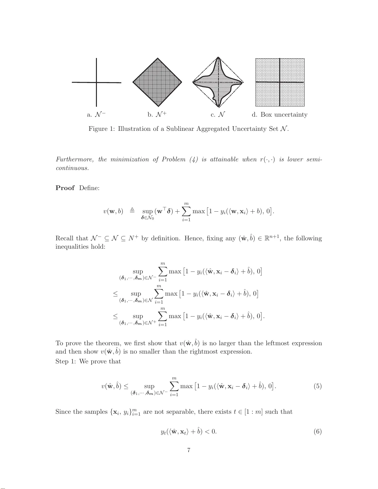
R obustness and Regulariza tion of SVMs Robustness and Re gularization of Supp ort V ector Mac hines Huan Xu xuhuan@cim.mcgill.ca , Dep a rtment o f Ele ctric al and Computer Engine ering, McGil l University, Canada Constan tine Caramanis cmcaram@ece.utexas.edu Dep a rtment of Ele ctric al and Computer Engine ering, The U niversity of T ex as at Austin, USA Shie Mannor shie.mannor@mcgill.ca Dep a rtment of Ele ctric al and Computer Engine ering, McGil l University, Canada Editor: Alexander Smola Abstract W e consider regularized suppo rt vector machines (SVMs) and show that they are precisely equiv alen t to a new robust optimization formulation. W e show that this equiv alence of robust optimization and regula rization ha s implications for b oth algo rithms, and analysis . In terms of alg orithms, the equiv ale nc e suggests more genera l SVM-lik e alg orithms for classification that explicitly build in protection to noise, and a t the same time control ov erfitting. On the analysis front, the equiv alence of robustness and regular ization, provides a r obust o ptimization interpretation for the s uccess of re g ularized SVMs. W e use the this new r obustness in terpretation of SVMs to give a new pro o f o f co nsistency of (kernelized) SVMs, thus establishing r obustness as the r e ason regulariz e d SVMs genera liz e w ell. Keyw ords: Robustness, Regularization, Generalization, K ernel, Suppor t V ector Machine 1. In tro duction Supp ort V ector Mac hines (SVMs for short) originated in Boser et al. (1992) and can b e traced bac k to as early as V apnik and Lerner (1963) and V apnik and Chervo nenkis (1974). They con tin ue to b e one of th e most successful algo rithms for classifica tion. SVMs ad- dress the classificati on p roblem b y finding th e h yp erp lane in the feature sp ace that ac hiev es maxim um samp le margin when the training s amples are separable, whic h leads to mini- mizing the norm of the classifier. When the samples are not separable, a p enalt y term that appro ximates the total training error is considered (Bennett and Mangasarian, 1992; Cortes and V apn ik, 1995). It is well kno wn that minimizing th e training err or itself can lead to p o or classification p erformance for new un lab eled data; that is, su c h an approac h ma y ha ve p oor generaliza tion error b ecause of, essen tially , ov erfitting (V apnik and Cherv onenk is, 1991). A v ariet y of mo d ifications hav e b een prop osed to com bat this problem, one of the most p opu lar metho ds b eing that of min imizing a com b ination of the trainin g-error and a regularization term. The latter is t ypically c h osen as a norm of the classifier. The resulting regularized classifier p erforms b ette r on new data. This p henomenon is often in terp reted from a statistic al learning theory view: the regularization term restricts the complexit y of the classifier, h ence the deviation of the testing error and the training error is con trolled (see Smola et al., 1998; Evgeniou et al. , 2000; Bartlet t and Mendelson, 2002; Koltc hinskii and Panc henko, 2002; Bartlet t et al., 2005, and references therein). 1 Xu, Caram anis and Mannor In this pap er w e consid er a different setup, assuming that the training d ata are gen- erated b y th e tru e underlying distribution, but some non-i.i.d. (p oten tially adversarial) disturbance is then add ed to the samples w e observe. W e follo w a robu st optimization (see El Ghaoui and Lebr et, 1997; Ben-T al and Nemiro vski, 1999; Bertsimas and S im, 2004, and r eferences therein) approac h, i.e., minimizing th e w orst p ossible empirical error un- der s uc h distu rbances. The use of robust optimizat ion in classificatio n is not new (e.g., Shiv asw am y et al., 2006; Bhattac hary ya et al., 2004b ; Lanc kriet et al., 2002). Robust clas- sification mo dels studied in the past ha ve considered only b o x-t yp e uncertain ty sets, whic h allo w the p ossibilit y that the data ha ve all b een skew ed in some non-neutral manner by a correlated distur bance. This has m ade it d ifficult to obtain n on -conserv ativ e generaliza tion b ound s. Mo reo ver, there has not b een an explicit connection to the regularized classi- fier, although at a h igh-lev el it is kno w n that regularization and robust optimization are related (e.g., El Ghaoui and Lebret, 1997; Ant hon y and Bartlett, 1999). The main contri- bution in this pap er is solving the robu st classificatio n p roblem for a class of non-b o x-t yp ed uncertain ty sets, and pr o vidin g a link age b et we en robust classificatio n and the stand ard regularization scheme of SVMs. In particular, our con tribu tions include the follo w ing: • W e solv e the rob u st S VM formula tion for a class of non-b o x-t yp e uncertain t y sets. This p ermits finer con trol of the adv er s arial disturbance, r estricting it to satisfy ag- gregate constrain ts across data p oint s, therefore reducing the p ossibilit y of highly correlated d isturbance. • W e sho w that the standard regularized SVM classifier is a sp ecial case of our robust classification, thus explicitly r elating robus tn ess and regularization. This pro vides an alternativ e explanation to the su ccess of regularization, and also suggests new physic ally motiv ated w ays to construct regularization terms. • W e relate our robust form u lation to sev eral pr obabilistic form u lations. W e consider a c han ce-constrained classifier (i.e., a classifier with prob ab ilistic constraints on mis- classification) and sho w that our robust form u lation can app ro ximate it far less con- serv ative ly than previous robust form ulations could p ossibly do. W e also consider a Ba yesian setup, and sho w that th is can b e used to pr o vide a p rincipled m eans of selecting the regularization co efficient w ithout cross-v alidation. • W e sho w that the robus tness p ersp ectiv e, stemming from a n on-i.i.d. analysis, can b e useful in th e standard learning (i.i.d.) setup, b y using it to pro ve consistency for standard SVM classificatio n, without u si ng VC-dimension or stability ar gu ments . This result implies that generalizati on abilit y is a d irect result of robustness to local disturbances; it therefore suggests a new justifi cation for go o d p erformance, and conse- quen tly allo ws us to construct learning algo rithms that generalize well by robus tifying non-consisten t algorithms. R ob ustnes s and R egulariza tion W e commen t h ere on the explicit equiv alence of robustness and regularizatio n. W e b r iefly ex- plain ho w this observ ation is different f rom p revious w ork and wh y it is inte resting. Certain equiv alence relationships b et we en robustn ess and regularization ha v e b een established for 2 R obustness and Regulariza tion of S VMs problems other than classification (El Ghaoui and Lebret, 1997; Ben-T al and Nemiro vski, 1999; Bishop, 1995), but their r esults do not dir ectly apply to the classification prob - lem. Indeed, researc h on classifier regularization mainly discusses its effect on b ound- ing the complexit y of the fun ction class (e.g., Smola et al., 1998; Evgeniou et al., 2000; Bartlett and Mendelson, 2002; Koltc hinskii and P anchenk o, 2002; Bartlett et al., 2005). Mean- while, researc h on r ob u st classification has not attempted to relate r obustness and regular- ization (e.g ., Lanc kriet et al., 2002; Bhattac h aryy a et al., 2004 a ,b; Shiv aswam y et al., 2006; T rafalis and Gilbert, 2007; Glob erson and R ow eis, 2006), in part d ue to the robustness for- m u lations used in those pap ers. In fact, they all consider r obustified v ers ions of r e gularize d classifications. 1 Bhattac h aryy a (2004) considers a robust form ulation for b o x-t yp e uncer- tain t y , and relate s this robu st formulati on with regularized SVM. Ho wev er, this form u lation in volv es a non-standard loss f u nction that do es not b ound the 0 − 1 loss, and hence its ph ys- ical interpretation is not clear. The connection of robustness and regularization in the SVM con text is imp ortant for the follo wing reasons. First, it give s an alternativ e and p oten tially p o werful explanation of the generalizat ion abilit y of the regularization term. In the classica l mac hine learning literature, the r egularization term b ound s the complexit y of the class of classifiers. The r obust view of regularization regards th e testing samples as a p erturb ed copy of the training samples. W e show that when the total p erturbation is giv en or b ounded, the regularizatio n term b ound s the gap b et ween the classification errors of the SVM on these t w o sets of samples. In con trast to th e standard P A C approac h, this b ound dep end s n either on ho w rich the class of candidate classifiers is, nor on an assumption that all samples are pic k ed in an i.i.d. manner. In addition, this su ggests nov el approac hes to designing go o d classification algorithms, in particular, designing the regularization term. In the P A C structural-risk minimization approac h , regularizatio n is chosen to minimize a b oun d on the generalization error based on the training error and a complexit y term. This complexit y term typically leads to o verly emp hasizing the regularizer, and in deed th is approac h is kn o wn to often b e to o p essimistic (Kearns et al., 1997 ) for problems w ith more structur e. The robus t approac h offers another a ven ue. Since b oth noise and robustn ess are physica l pro cesses, a close inv estigatio n of the application and n oise c haracteristics at h and, can p ro vid e insigh ts in to ho w to prop erly robu stify , and therefore regularize the classifier. F or example, it is kno wn that normalizing the samples so that the v ariance among all features is roughly the same (a pro cess commonly used to eliminate the scaling fr eedom of individual features) often leads to goo d generaliza tion p erformance. F rom the robustness p ersp ectiv e, this simply says that the noise is anisotropic (ellipsoidal) rather than s p herical, and hence an approp r iate robustification m ust b e designed to fit this anisotrop y . W e also show that u sing th e robust optimiza tion viewp oin t, we obtain some probab ilistic results outside the P A C setup . In Section 3 we b ound the p robabilit y that a n oisy training sample is correctly lab eled. S uc h a b ound considers the b ehavior of c orrupte d samples and is hence differen t from the kn o wn P A C b ounds. This is h elpful when the training samples and the testing samples are dra wn from differen t distributions, or some adv ersary m an ip ulates the samples to p rev ent th em from b eing correctly lab eled (e.g., spam senders change th eir patterns from time to time to av oid b eing lab eled and filtered). Finally , this connection of 1. Lanc kriet et al. (2002) is p erhaps the only exception, where a regularization term is added to the cov ari- ance estimation rather than to the ob jective function. 3 Xu, Caram anis and Mannor robustification and regularization also pro vid es us with new pr o of tec h niques as w ell (see Section 5). W e need to p oin t out that there are several different definitions of r obustness in litera- ture. In th is p ap er, as well as the aforementio ned robust classificati on pap ers, robu stness is mainly un dersto o d fr om a Rob u st Op timization p ersp ectiv e, where a min-max optimiza- tion is p erform ed ov er all p ossib le d isturbances. An alternativ e inte rpretation of rob u stness stems from the rich literature on Robust Statistics (e.g., Hu b er, 1981; Hamp el et al., 1986; Rousseeu w and Leeroy, 1987 ; Maronna et al., 2006), wh ic h s tu dies ho w an estimator or algorithm b ehav es u nder a small p erturbation of the statistics mo del. F or example, the In- fluence F unction approac h, p rop osed in Hamp el (1974) and Hamp el et al. (1986), measures the impact of an infinitesimal amount of con tamination of th e original distribution on the quan tit y of in terest. Based on th is notion of robu stness, Christmann and Steinw art (2004) sho wed that many kernel classifica tion algorithms, including SVM, are robust in the sense of ha ving a fi nite Influ ence F unction. A similar resu lt for regression algorithms is sho wn in Christmann and Stein w art (20 07) for s mo oth loss functions, and in Christmann and V an Messem (2008) for non-smo oth loss functions where a relaxed version of th e Influ ence F unction is applied. In the m ac hine learning literature, another widely used notion closely related to robustness is the stability , wh er e an algorithm is required to b e robu s t (in the s en se that the output f unction do es n ot c hange significan tly) under a s p ecific p erturbation: deleting one sample from the training set. It is n o w w ell kno wn that a stable algorithm suc h as SVM has d esirable generaliza tion p rop erties, and is statistic ally consistent u nder mild tec h - nical conditions; see for example Bousquet and Elisseeff (2002); Kutin and Niy ogi (2002); P oggio et al. (2004); Mukherj ee et al. (2006) for details. One main difference b etw een Ro- bust Op timization and other r obustness n otions is that the former is constru ctiv e r ather than analytical. That is, in con tr ast to r obust statistics or the stabilit y ap p roac h th at mea- sures the robu stness of a given algorithm, Robust O p timization can r obustify an algorithm: it con verts a giv en algorithm to a robust one. F or example, as we sho w in this pap er, the R O v ersion of a naiv e empirical-e rror minimization is the well kno wn SVM. As a constructiv e pro cess, the RO appr oac h also leads to additional flexibilit y in algorithm design, esp ecially when the nature of the p ertu rbation is kno wn or can b e wel l estimated. Structure of the Paper: This pap er is organized as follo ws. In Section 2 w e in vesti gate the correlated disturbance case, and sho w the equiv alence b et w een the r obust classificatio n and the regularization pro cess. W e deve lop the conn ections to pr obabilistic formulat ions in Section 3, and pro ve a consistency result based on robustness analysis in Section 5. The kernelize d v ersion is in v estigated in Section 4. Some concluding remarks are giv en in Section 6. Notation: C apital letters are used to den ote matrices, and b oldface letters are us ed to denote column v ectors. F or a giv en n orm k · k , w e u se k · k ∗ to denote its dual norm, i.e., k z k ∗ , su p { z ⊤ x |k x k ≤ 1 } . F or a v ector x and a p ositiv e semi-definite matrix C of the same dimension, k x k C denotes √ x ⊤ C x . W e use δ to denote d isturbance affecting th e samples. W e u se su p ers cr ip t r to denote the tr ue v alue for an uncertain v ariable, so that δ r i is the true (but unkn o wn ) noise of the i th sample. The set of non-negativ e scalars is denoted b y R + . The set of in tegers from 1 to n is den oted by [1 : n ]. 4 R obustness and Regulariza tion of S VMs 2. Robust Classification and Regularization W e consider the s tand ard binary classification problem, w h ere w e are given a finite num b er of trainin g samp les { x i , y i } m i =1 ⊆ R n × {− 1 , +1 } , and m u st find a linear classifier, sp ecified b y the function h w ,b ( x ) = sgn( h w , x i + b ) . F or the standard regularized classifier, the parameters ( w , b ) are obtained b y solving the follo win g con ve x optimizatio n p roblem: min w ,b, ξ : r ( w , b ) + m X i =1 ξ i s . t . : ξ i ≥  1 − y i ( h w , x i i + b )] ξ i ≥ 0 , where r ( w , b ) is a regularization term. This is equiv alent to min w ,b ( r ( w , b ) + m X i =1 max  1 − y i ( h w , x i i + b ) , 0  ) . Previous robust classificati on work (S hiv asw amy et al., 2006; Bhattac h aryy a et al., 2004a,b; Bhattac h aryy a , 2004; T rafalis and Gilb ert, 2007) considers th e classifica tion problem where the input are sub ject to (u n kno wn) disturbances ~ δ = ( δ 1 , . . . , δ m ) and essen tially solves the follo wing min-max p roblem: min w ,b max ~ δ ∈N b o x ( r ( w , b ) + m X i =1 max  1 − y i ( h w , x i − δ i i + b ) , 0  ) , (1) for a b ox-t yp e un certain t y set N b o x . Th at is, let N i denotes the pr o jection of N b o x on to the δ i comp onent , then N b o x = N 1 × · · · × N m . Effecti v ely , this allo ws sim ultaneous w orst- case disturbances across man y samples, and leads to o verly conserv ativ e solutions. The goal of this pap er is to obtain a robust form u lation w here the distu rbances { δ i } ma y b e meaningfully tak en to b e correlated, i.e., to s olve for a non-b o x-t yp e N : min w ,b max ~ δ ∈N ( r ( w , b ) + m X i =1 max  1 − y i ( h w , x i − δ i i + b ) , 0  ) . (2) W e briefly exp lain here the four reasons that motiv ate this “robu s t to p erturbation” setup and in particular the min -max form of (1) and (2). First, it can explicitly in corp orate prior problem kn o wledge of local in v ariance (e.g, T eo et al., 2008). F or example, in v ision tasks, a desir ab le classifier s hould p ro vid e a consisten t answ er if an in put im age sligh tly change s. Second, there are situations where some adv ersarial opp on ents (e.g., spam senders) w ill manipulate the testing samples to av oid b eing corr ectly classified, and th e robustness to- w ard su c h manipu lation should b e tak en into consideration in the training pro cess (e.g, Glob erson and Ro weis, 2006). O r alte rnativ ely , the training samples and the testing sam- ples can b e obtained from differen t pr o cesses and hence the standard i.i.d. assump tion is violated (e.g, Bi and Zh ang, 2004). F or example in real-time applications, the newly gener- ated samples are often less accurate due to time constrain ts. Finally , formulat ions b ased on c hance-constrain ts (e.g., Bhattac haryya et al., 2004b; Shiv asw amy et al., 2006) are mathe- matically equiv alen t to suc h a min-max form ulation. W e define explicitly the correlated distu rbance (or uncertain t y) wh ich w e study b elo w . 5 Xu, Caram anis and Mannor Definition 1 A se t N 0 ⊆ R n is c al le d an A tomic Uncertain ty Set if (I) 0 ∈ N 0 ; (II) F or any w 0 ∈ R n : sup δ [ w ⊤ 0 δ ] = sup δ ′ [ − w ⊤ 0 δ ′ ] < + ∞ . W e u se “sup” here b ecause the maximal v alue is not necessary attained since N 0 ma y not b e a closed set. The second condition of A tomic Uncertain t y set basically sa ys that the uncertain ty set is b ounded and sym metric. In particular, all n orm balls and ellipsoids cen tered at the origin are atomic uncertain ty sets, while an arbitrary p olytop e migh t n ot b e an atomic un certain ty set. Definition 2 L et N 0 b e an atomic u nc ertainty set. A set N ⊆ R n × m is c al le d a Su blinear Aggregat ed Uncertaint y Set of N 0 , if N − ⊆ N ⊆ N + , wher e: N − , m [ t =1 N − t ; N − t , { ( δ 1 , · · · , δ m ) | δ t ∈ N 0 ; δ i 6 = t = 0 } . N + , { ( α 1 δ 1 , · · · , α m δ m ) | m X i =1 α i = 1; α i ≥ 0 , δ i ∈ N 0 , i = 1 , · · · , m } . The Sublinear Aggregate d Uncertain t y defin ition mo dels the case where the d isturbances on eac h samp le are treated ident ically , bu t their aggreg ate b eha vior across m ultiple samples is con trolled. Some in teresting examples in clude (1) { ( δ 1 , · · · , δ m ) | m X i =1 k δ i k ≤ c } ; (2) { ( δ 1 , · · · , δ m ) |∃ t ∈ [1 : m ]; k δ t k ≤ c ; δ i = 0 , ∀ i 6 = t } ; (3) { ( δ 1 , · · · , δ m ) | m X i =1 p c k δ i k ≤ c } . All th ese examples h a ve the same atomic uncertain t y set N 0 =  δ   k δ k ≤ c  . Figure 1 pro v id es an illustration of a sublin ear aggregated u ncertain ty set for n = 1 and m = 2, i.e., the trainin g set consists of t wo u niv ariate samples. Theorem 3 A ssume { x i , y i } m i =1 ar e non-sep ar able, r ( · ) : R n +1 → R is an arbitr ary fu nc - tion, N is a Subline ar A gg r e gate d Unc e rtainty set with c orr esp onding atomic unc ertainty set N 0 . Then the fol lowing min-max pr oblem min w ,b sup ( δ 1 , ··· , δ m ) ∈N ( r ( w , b ) + m X i =1 max  1 − y i ( h w , x i − δ i i + b ) , 0  ) (3) is e quivalent to the f ol lowing optimization pr oblem on w , b, ξ : min : r ( w , b ) + sup δ ∈N 0 ( w ⊤ δ ) + m X i =1 ξ i , s . t . : ξ i ≥ 1 − [ y i ( h w , x i i + b )] , i = 1 , . . . , m ; ξ i ≥ 0 , i = 1 , . . . , m. (4) 6 R obustness and Regulariza tion of S VMs xxxxxxxxxxxxxxxxxxxxxxxxxxxxxxxxxxxxxxxxxxxxxxxxxxxxxxxxx xxxxxxxxxxxxxxxxxxxxxxxxxxxxxxxxxxxxxxxxxxxxxxxxxxxxxxxxx xxxxxxxxxxxxxxxxxxxxxxxxxxxxxxxxxxxxxxxxxxxxxxxxxxxxxxxxx xxxxxxxxxxxxxxxxxxxxxxxxxxxxxxxxxxxxxxxxxxxxxxxxxxxxxxxxx xxxxxxxxxxxxxxxxxxxxxxxxxxxxxxxxxxxxxxxxxxxxxxxxxxxxxxxxx xxxxxxxxxxxxxxxxxxxxxxxxxxxxxxxxxxxxxxxxxxxxxxxxxxxxxxxxx xxxxxxxxxxxxxxxxxxxxxxxxxxxxxxxxxxxxxxxxxxxxxxxxxxxxxxxxx xxxxxxxxxxxxxxxxxxxxxxxxxxxxxxxxxxxxxxxxxxxxxxxxxxxxxxxxx xxxxxxxxxxxxxxxxxxxxxxxxxxxxxxxxxxxxxxxxxxxxxxxxxxxxxxxxx xxxxxxxxxxxxxxxxxxxxxxxxxxxxxxxxxxxxxxxxxxxxxxxxxxxxxxxxx xxxxxxxxxxxxxxxxxxxxxxxxxxxxxxxxxxxxxxxxxxxxxxxxxxxxxxxxx xxxxxxxxxxxxxxxxxxxxxxxxxxxxxxxxxxxxxxxxxxxxxxxxxxxxxxxxx xxxxxxxxxxxxxxxxxxxxxxxxxxxxxxxxxxxxxxxxxxxxxxxxxxxxxxxxx xxxxxxxxxxxxxxxxxxxxxxxxxxxxxxxxxxxxxxxxxxxxxxxxxxxxxxxxx xxxxxxxxxxxxxxxxxxxxxxxxxxxxxxxxxxxxxxxxxxxxxxxxxxxxxxxxx xxxxxxxxxxxxxxxxxxxxxxxxxxxxxxxxxxxxxxxxxxxxxxxxxxxxxxxxx xxxxxxxxxxxxxxxxxxxxxxxxxxxxxxxxxxxxxxxxxxxxxxxxxxxxxxxxx xxxxxxxxxxxxxxxxxxxxxxxxxxxxxxxxxxxxxxxxxxxxxxxxxxxxxxxxx xxxxxxxxxxxxxxxxxxxxxxxxxxxxxxxxxxxxxxxxxxxxxxxxxxxxxxxxx xxxxxxxxxxxxxxxxxxxxxxxxxxxxxxxxxxxxxxxxxxxxxxxxxxxxxxxxx xxxxxxxxxxxxxxxxxxxxxxxxxxxxxxxxxxxxxxxxxxxxxxxxxxxxxxxxx xxxxxxxxxxxxxxxxxxxxxxxxxxxxxxxxxxxxxxxxxxxxxxxxxxxxxxxxx xxxxxxxxxxxxxxxxxxxxxxxxxxxxxxxxxxxxxxxxxxxxxxxxxxxxxxxxx xxxxxxxxxxxxxxxxxxxxxxxxxxxxxxxxxxxxxxxxxxxxxxxxxxxxxxxxx xxxxxxxxxxxxxxxxxxxxxxxxxxxxxxxxxxxxxxxxxxxxxxxxxxxxxxxxx xxxxxxxxxxxxxxxxxxxxxxxxxxxxxxxxxxxxxxxxxxxxxxxxxxxxxxxxx xxxxxxxxxxxxxxxxxxxxxxxxxxxxxxxxxxxxxxxxxxxxxxxxxxxxxxxxx xxxxxxxxxxxxxxxxxxxxxxxxxxxxxxxxxxxxxxxxxxxxxxxxxxxxxxxxx xxxxxxxxxxxxxxxxxxxxxxxxxxxxxxxxxxxxxxxxxxxxxxxxxxxxxxxxx xxxxxxxxxxxxxxxxxxxxxxxxxxxxxxxxxxxxxxxxxxxxxxxxxxxxxxxxx xxxxxxxxxxxxxxxxxxxxxxxxxxxxxxxxxxxxxxxxxxxxxxxxxxxxxxxxx xxxxxxxxxxxxxxxxxxxxxxxxxxxxxxxxxxxxxxxxxxxxxxxxxxxxxxxxx xxxxxxxxxxxxxxxxxxxxxxxxxxxxxxxxxxxxxxxxxxxxxxxxxxxxxxxxx xxxxxxxxxxxxxxxxxxxxxxxxxxxxxxxxxxxxxxxxxxxxxxxxxxxxxxxxx xxxxxxxxxxxxxxxxxxxxxxxxxxxxxxxxxxxxxxxxxxxxxxxxxxxxxxxxx xxxxxxxxxxxxxxxxxxxxxxxxxxxxxxxxxxxxxxxxxxxxxxxxxxxxxxxxx xxxxxxxxxxxxxxxxxxxxxxxxxxxxxxxxxxxxxxxxxxxxxxxxxxxxxxxxx xxxxxxxxxxxxxxxxxxxxxxxxxxxxxxxxxxxxxxxxxxxxxxxxxxxxxxxxx xxxxxxxxxxxxxxxxxxxxxxxxxxxxxxxxxxxxxxxxxxxxxxxxxxxxxxxxx xxxxxxxxxxxxxxxxxxxxxxxxxxxxxxxxxxxxxxxxxxxxxxxxxxxxxxxxx xxxxxxxxxxxxxxxxxxxxxxxxxxxxxxxxxxxxxxxxxxxxxxxxxxxxxxxxx xxxxxxxxxxxxxxxxxxxxxxxxxxxxxxxxxxxxxxxxxxxxxxxxxxxxxxxxx xxxxxxxxxxxxxxxxxxxxxxxxxxxxxxxxxxxxxxxxxxxxxxxxxxxxxxxxx xxxxxxxxxxxxxxxxxxxxxxxxxxxxxxxxxxxxxxxxxxxxxxxxxxxxxxxxx xxxxxxxxxxxxxxxxxxxxxxxxxxxxxxxxxxxxxxxxxxxxxxxxxxxxxxxxx xxxxxxxxxxxxxxxxxxxxxxxxxxxxxxxxxxxxxxxxxxxxxxxxxxxxxxxxx xxxxxxxxxxxxxxxxxxxxxxxxxxxxxxxxxxxxxxxxxxxxxxxxxxxxxxxxx xxxxxxxxxxxxxxxxxxxxxxxxxxxxxxxxxxxxxxxxxxxxxxxxxxxxxxxxx xxxxxxxxxxxxxxxxxxxxxxxxxxxxxxxxxxxxxxxxxxxxxxxxxxxxxxxxx xxxxxxxxxxxxxxxxxxxxxxxxxxxxxxxxxxxxxxxxxxxxxxxxxxxxxxxxx xxxxxxxxxxxxxxxxxxxxxxxxxxxxxxxxxxxxxxxxxxxxxxxxxxxxxxxxx xxxxxxxxxxxxxxxxxxxxxxxxxxxxxxxxxxxxxxxxxxxxxxxxxxxxxxxxx xxxxxxxxxxxxxxxxxxxxxxxxxxxxxxxxxxxxxxxxxxxxxxxxxxxxxxxxx xxxxxxxxxxxxxxxxxxxxxxxxxxxxxxxxxxxxxxxxxxxxxxxxxxxxxxxxx xxxxxxxxxxxxxxxxxxxxxxxxxxxxxxxxxxxxxxxxxxxxxxxxxxxxxxxxx xxxxxxxxxxxxxxxxxxxxxxxxxxxxxxxxxxxxxxxxxxxxxxxxxxxxxxxxx xxxxxxxxxxxxxxxxxxxxxxxxxxxxxxxxxxxxxxxxxxxxxxxxxxxxxxxxx xxxxxxxxxxxxxxxxxxxxxxxxxxxxxxxxxxxxxxxxxxxxxxxxxxxxx xxxxxxxxxxxxxxxxxxxxxxxxxxxxxxxxxxxxxxxxxxxxxxxxxxxxx xxxxxxxxxxxxxxxxxxxxxxxxxxxxxxxxxxxxxxxxxxxxxxxxxxxxx xxxxxxxxxxxxxxxxxxxxxxxxxxxxxxxxxxxxxxxxxxxxxxxxxxxxx xxxxxxxxxxxxxxxxxxxxxxxxxxxxxxxxxxxxxxxxxxxxxxxxxxxxx xxxxxxxxxxxxxxxxxxxxxxxxxxxxxxxxxxxxxxxxxxxxxxxxxxxxx xxxxxxxxxxxxxxxxxxxxxxxxxxxxxxxxxxxxxxxxxxxxxxxxxxxxx xxxxxxxxxxxxxxxxxxxxxxxxxxxxxxxxxxxxxxxxxxxxxxxxxxxxx xxxxxxxxxxxxxxxxxxxxxxxxxxxxxxxxxxxxxxxxxxxxxxxxxxxxx xxxxxxxxxxxxxxxxxxxxxxxxxxxxxxxxxxxxxxxxxxxxxxxxxxxxx xxxxxxxxxxxxxxxxxxxxxxxxxxxxxxxxxxxxxxxxxxxxxxxxxxxxx xxxxxxxxxxxxxxxxxxxxxxxxxxxxxxxxxxxxxxxxxxxxxxxxxxxxx xxxxxxxxxxxxxxxxxxxxxxxxxxxxxxxxxxxxxxxxxxxxxxxxxxxxx xxxxxxxxxxxxxxxxxxxxxxxxxxxxxxxxxxxxxxxxxxxxxxxxxxxxx xxxxxxxxxxxxxxxxxxxxxxxxxxxxxxxxxxxxxxxxxxxxxxxxxxxxx xxxxxxxxxxxxxxxxxxxxxxxxxxxxxxxxxxxxxxxxxxxxxxxxxxxxx xxxxxxxxxxxxxxxxxxxxxxxxxxxxxxxxxxxxxxxxxxxxxxxxxxxxx xxxxxxxxxxxxxxxxxxxxxxxxxxxxxxxxxxxxxxxxxxxxxxxxxxxxx xxxxxxxxxxxxxxxxxxxxxxxxxxxxxxxxxxxxxxxxxxxxxxxxxxxxx xxxxxxxxxxxxxxxxxxxxxxxxxxxxxxxxxxxxxxxxxxxxxxxxxxxxx xxxxxxxxxxxxxxxxxxxxxxxxxxxxxxxxxxxxxxxxxxxxxxxxxxxxx xxxxxxxxxxxxxxxxxxxxxxxxxxxxxxxxxxxxxxxxxxxxxxxxxxxxx xxxxxxxxxxxxxxxxxxxxxxxxxxxxxxxxxxxxxxxxxxxxxxxxxxxxx xxxxxxxxxxxxxxxxxxxxxxxxxxxxxxxxxxxxxxxxxxxxxxxxxxxxx xxxxxxxxxxxxxxxxxxxxxxxxxxxxxxxxxxxxxxxxxxxxxxxxxxxxx xxxxxxxxxxxxxxxxxxxxxxxxxxxxxxxxxxxxxxxxxxxxxxxxxxxxx xxxxxxxxxxxxxxxxxxxxxxxxxxxxxxxxxxxxxxxxxxxxxxxxxxxxx xxxxxxxxxxxxxxxxxxxxxxxxxxxxxxxxxxxxxxxxxxxxxxxxxxxxx xxxxxxxxxxxxxxxxxxxxxxxxxxxxxxxxxxxxxxxxxxxxxxxxxxxxx xxxxxxxxxxxxxxxxxxxxxxxxxxxxxxxxxxxxxxxxxxxxxxxxxxxxx xxxxxxxxxxxxxxxxxxxxxxxxxxxxxxxxxxxxxxxxxxxxxxxxxxxxx xxxxxxxxxxxxxxxxxxxxxxxxxxxxxxxxxxxxxxxxxxxxxxxxxxxxx xxxxxxxxxxxxxxxxxxxxxxxxxxxxxxxxxxxxxxxxxxxxxxxxxxxxx xxxxxxxxxxxxxxxxxxxxxxxxxxxxxxxxxxxxxxxxxxxxxxxxxxxxx xxxxxxxxxxxxxxxxxxxxxxxxxxxxxxxxxxxxxxxxxxxxxxxxxxxxx xxxxxxxxxxxxxxxxxxxxxxxxxxxxxxxxxxxxxxxxxxxxxxxxxxxxx xxxxxxxxxxxxxxxxxxxxxxxxxxxxxxxxxxxxxxxxxxxxxxxxxxxxx xxxxxxxxxxxxxxxxxxxxxxxxxxxxxxxxxxxxxxxxxxxxxxxxxxxxx xxxxxxxxxxxxxxxxxxxxxxxxxxxxxxxxxxxxxxxxxxxxxxxxxxxxx xxxxxxxxxxxxxxxxxxxxxxxxxxxxxxxxxxxxxxxxxxxxxxxxxxxxx xxxxxxxxxxxxxxxxxxxxxxxxxxxxxxxxxxxxxxxxxxxxxxxxxxxxx xxxxxxxxxxxxxxxxxxxxxxxxxxxxxxxxxxxxxxxxxxxxxxxxxxxxx xxxxxxxxxxxxxxxxxxxxxxxxxxxxxxxxxxxxxxxxxxxxxxxxxxxxx xxxxxxxxxxxxxxxxxxxxxxxxxxxxxxxxxxxxxxxxxxxxxxxxxxxxx xxxxxxxxxxxxxxxxxxxxxxxxxxxxxxxxxxxxxxxxxxxxxxxxxxxxx xxxxxxxxxxxxxxxxxxxxxxxxxxxxxxxxxxxxxxxxxxxxxxxxxxxxx xxxxxxxxxxxxxxxxxxxxxxxxxxxxxxxxxxxxxxxxxxxxxxxxxxxxx xxxxxxxxxxxxxxxxxxxxxxxxxxxxxxxxxxxxxxxxxxxxxxxxxxxxx xxxxxxxxxxxxxxxxxxxxxxxxxxxxxxxxxxxxxxxxxxxxxxxxxxxxx xxxxxxxxxxxxxxxxxxxxxxxxxxxxxxxxxxxxxxxxxxxxxxxxxxxxx xxxxxxxxxxxxxxxxxxxxxxxxxxxxxxxxxxxxxxxxxxxxxxxxxxxxx xxxxxxxxxxxxxxxxxxxxxxxxxxxxxxxxxxxxxxxxxxxxxxxxxxxxx xxxxxxxxxxxxxxxxxxxxxxxxxxxxxxxxxxxxxxxxxxxxxxxxxxxxx xxxxxxxxxxxxxxxxxxxxxxxxxxxxxxxxxxxxxxxxxxxxxxxxxxxxx xxxxxxxxxxxxxxxxxxxxxxxxxxxxxxxxxxxxxxxxxxxxxxxxxxxxx xxxxxxxxxxxxxxxxxxxxxxxxxxxxxxxxxxxxxxxxxxxxxxxxxxxxx xxxxxxxxxxxxxxxxxxxxxxxxxxxxxxxxxxxxxxxxxxxxxxxxxxxxx xxxxxxxxxxxxxxxxxxxxxxxxxxxxx xxxxxxxxxxxxxxxxxxxxxxxxxxxxx xxxxxxxxxxxxxxxxxxxxxxxxxxxxx xxxxxxxxxxxxxxxxxxxxxxxxxxxxx xxxxxxxxxxxxxxxxxxxxxxxxxxxxx xxxxxxxxxxxxxxxxxxxxxxxxxxxxx xxxxxxxxxxxxxxxxxxxxxxxxxxxxx xxxxxxxxxxxxxxxxxxxxxxxxxxxxx xxxxxxxxxxxxxxxxxxxxxxxxxxxxx xxxxxxxxxxxxxxxxxxxxxxxxxxxxx xxxxxxxxxxxxxxxxxxxxxxxxxxxxx xxxxxxxxxxxxxxxxxxxxxxxxxxxxx xxxxxxxxxxxxxxxxxxxxxxxxxxxxx xxxxxxxxxxxxxxxxxxxxxxxxxxxxx xxxxxxxxxxxxxxxxxxxxxxxxxxxxx xxxxxxxxxxxxxxxxxxxxxxxxxxxxx xxxxxxxxxxxxxxxxxxxxxxxxxxxxx xxxxxxxxxxxxxxxxxxxxxxxxxxxxx xxxxxxxxxxxxxxxxxxxxxxxxxxxxx xxxxxxxxxxxxxxxxxxxxxxxxxxxxx xxxxxxxxxxxxxxxxxxxxxxxxxxxxx xxxxxxxxxxxxxxxxxxxxxxxxxxxxx xxxxxxxxxxxxxxxxxxxxxxxxxxxxx xxxxxxxxxxxxxxxxxxxxxxxxxxxxx xxxxxxxxxxxxxxxxxxxxxxxxxxxxx xxxxxxxxxxxxxxxxxxxxxxxxxxxxx xxxxxxxxxxxxxxxxxxxxxxxxxxxxx xxxxxxxxxxxxxxxxxxxxxxxxxxxxx xxxxxxxxxxxxxxxxxxxxxxxxxxxxx xxxxxxxxxxxxxxxxxxxxxxxxxxxxx a. N − b. N + c. N d. Bo x uncertain ty Figure 1: Illustration of a Sublinear Aggregated Uncertain ty Set N . F urthermor e, the minimization of Pr oblem (4) i s attainable when r ( · , · ) i s lower semi- c ontinuous. Pro of Define: v ( w , b ) , sup δ ∈N 0 ( w ⊤ δ ) + m X i =1 max  1 − y i ( h w , x i i + b ) , 0  . Recall that N − ⊆ N ⊆ N + b y d efinition. Hence, fixing an y ( ˆ w , ˆ b ) ∈ R n +1 , the follo win g inequalities hold: sup ( δ 1 , ··· , δ m ) ∈N − m X i =1 max  1 − y i ( h ˆ w , x i − δ i i + ˆ b ) , 0  ≤ sup ( δ 1 , ··· , δ m ) ∈N m X i =1 max  1 − y i ( h ˆ w , x i − δ i i + ˆ b ) , 0  ≤ sup ( δ 1 , ··· , δ m ) ∈N + m X i =1 max  1 − y i ( h ˆ w , x i − δ i i + ˆ b ) , 0  . T o pro ve the theorem, we fi rst sho w that v ( ˆ w , ˆ b ) is no larger than the leftmost expression and then sho w v ( ˆ w , ˆ b ) is no smaller than the righ tmost expression. Step 1: W e p ro ve that v ( ˆ w , ˆ b ) ≤ sup ( δ 1 , ··· , δ m ) ∈N − m X i =1 max  1 − y i ( h ˆ w , x i − δ i i + ˆ b ) , 0  . (5) Since the samples { x i , y i } m i =1 are not separable, there exists t ∈ [1 : m ] suc h that y t ( h ˆ w , x t i + ˆ b ) < 0 . (6) 7 Xu, Caram anis and Mannor Hence, sup ( δ 1 , ··· , δ m ) ∈N − t m X i =1 max  1 − y i ( h ˆ w , x i − δ i i + ˆ b ) , 0  = X i 6 = t max  1 − y i ( h ˆ w , x i i + ˆ b ) , 0  + sup δ t ∈N 0 max  1 − y t ( h ˆ w , x t − δ t i + ˆ b ) , 0  = X i 6 = t max  1 − y i ( h ˆ w , x i i + ˆ b ) , 0  + max  1 − y t ( h ˆ w , x t i + ˆ b ) + sup δ t ∈N 0 ( y t ˆ w ⊤ δ t ) , 0  = X i 6 = t max  1 − y i ( h ˆ w , x i i + ˆ b ) , 0  + max  1 − y t ( h ˆ w , x t i + ˆ b ) , 0  + sup δ t ∈N 0 ( y t ˆ w ⊤ δ t ) = su p δ ∈N 0 ( ˆ w ⊤ δ ) + m X i =1 max  1 − y i ( h ˆ w , x i i + ˆ b ) , 0  = v ( ˆ w , ˆ b ) . The third equalit y h olds b ecause of In equ alit y (6) and sup δ t ∈N 0 ( y t ˆ w ⊤ δ t ) b eing non-negativ e (recall 0 ∈ N 0 ). Since N − t ⊆ N − , In equalit y (5) follo ws. Step 2: Next w e pro ve that sup ( δ 1 , ··· , δ m ) ∈N + m X i =1 max  1 − y i ( h ˆ w , x i − δ i i + ˆ b ) , 0  ≤ v ( ˆ w , ˆ b ) . (7) Notice that b y the defin ition of N + w e ha ve sup ( δ 1 , ··· , δ m ) ∈N + m X i =1 max  1 − y i ( h ˆ w , x i − δ i i + ˆ b ) , 0  = sup P m i =1 α i =1; α i ≥ 0; ˆ δ i ∈N 0 m X i =1 max  1 − y i ( h ˆ w , x i − α i ˆ δ i i + ˆ b ) , 0  = sup P m i =1 α i =1; α i ≥ 0; m X i =1 max  sup ˆ δ i ∈N 0  1 − y i ( h ˆ w , x i − α i ˆ δ i i + ˆ b )  , 0  . (8) No w, for any i ∈ [1 : m ], the follo wing holds, max  sup ˆ δ i ∈N 0  1 − y i ( h ˆ w , x i − α i ˆ δ i i + ˆ b )  , 0  = max  1 − y i ( h ˆ w , x i i + ˆ b ) + α i sup ˆ δ i ∈N 0 ( ˆ w ⊤ ˆ δ i ) , 0  ≤ max  1 − y i ( h ˆ w , x i i + ˆ b ) , 0  + α i sup ˆ δ i ∈N 0 ( ˆ w ⊤ ˆ δ i ) . Therefore, Equ ation (8) is upp er b oun ded b y m X i =1 max  1 − y i ( h ˆ w , x i i + ˆ b ) , 0  + sup P m i =1 α i =1; α i ≥ 0; m X i =1 α i sup ˆ δ i ∈N 0 ( ˆ w ⊤ ˆ δ i ) = sup δ ∈N 0 ( ˆ w ⊤ δ ) + m X i =1 max  1 − y i ( h ˆ w , x i i + ˆ b ) , 0  = v ( ˆ w , ˆ b ) , 8 R obustness and Regulariza tion of S VMs hence I n equalit y (7) holds. Step 3: Combining the tw o steps and adding r ( w , b ) on b oth sides leads to: ∀ ( w , b ) ∈ R n +1 , sup ( δ 1 , ··· , δ m ) ∈N m X i =1 max  1 − y i ( h w , x i − δ i i + b ) , 0  + r ( w , b ) = v ( w , b ) + r ( w , b ) . T aking the infimum on b oth sides establishes the equiv alence of Problem (3) and P r ob- lem (4) . Observe th at su p δ ∈N 0 w ⊤ δ is a su premum ov er a class of affine fu nctions, and hence is low er semi-con tinuous. Therefore v ( · , · ) is also lo wer s emi-con tinuous. Thus the minim um can b e ac hieved for Problem (4), and Problem (3) by equiv alence, when r ( · ) is lo we r semi-con tinuous. This th eorem rev eals the main difference b et w een F orm ulation (1) and our formulation in (2). Consider a Sublinear Aggregated Uncertain t y set N = { ( δ 1 , · · · , δ m ) | P m i =1 k δ i k ≤ c } . The smallest b o x-t yp e uncertain t y set con taining N includes disturban ces with norm sum up to mc . Therefore, it leads to a regularizatio n co efficien t as large as mc that is link ed to the n u m b er of training samples, and will therefore b e o ve rly conserv ative . An immediate corolla ry is that a sp ecial case of our robust form ulation is equiv alen t to the n orm-regularized SVM setup: Corollary 4 L et T , n ( δ 1 , · · · δ m ) | P m i =1 k δ i k ∗ ≤ c o . If the tr aining sample { x i , y i } m i =1 ar e non-sep ar able, then the fol lowing two optimization pr oblems on ( w , b ) ar e e quiv alent 2 min : max ( δ 1 , ··· , δ m ) ∈T m X i =1 max  1 − y i  h w , x i − δ i i + b  , 0  , (9) min : c k w k + m X i =1 max  1 − y i  h w , x i i + b  , 0  . (10) Pro of Let N 0 b e th e dual-norm ball { δ |k δ k ∗ ≤ c } and r ( w , b ) ≡ 0. Th en sup k δ k ∗ ≤ c ( w ⊤ δ ) = c k w k . Th e corollary follo w s from Th eorem 3. Notice indeed the equiv alence holds for an y w and b . This coroll ary explains the widely known fact that the r egularized classifier tend s to b e more robust. Sp ecifically , it explains the observ ation that wh en the disturb ance is noise- lik e and neutr al rather than adv ersarial, a norm-regularized classifier (without an y robust- ness requ iremen t) has a p erformance often sup erior to a b ox-typ e d robust classifier (see T rafalis and Gilbert, 2007). O n the other hand, this observ ation also suggests that the appropriate w a y to regularize sh ou ld come from a d istu rbance-robustness p ersp ectiv e. The ab o ve equ iv alence implies that standard regularization essential ly assumes th at the dis- turbance is sph erical; if this is not true, robustness may yield a b etter regularization-lik e algorithm. T o find a more effectiv e regularization term, a closer in vestig ation of the data v ariation is desirable, e.g., b y examining the v ariation of the data and solving the corre- sp ond ing robust classification p roblem. F or example, one wa y to r egularize is by splitting 2. The optimization equiv alence for the linear case wa s observed indep endently by Bertsimas and F ertis (2008). 9 Xu, Caram anis and Mannor the give n training samples into t wo sub sets with equ al num b er of elemen ts, and treating one as a disturb ed cop y of th e other. By analyzing the d irection of the d isturbance and the magnitude of the total v ariation, one can choose th e prop er norm to u se, and a suitable tradeoff parameter. 3. Probabilistic In t erpretations Although Problem (3) is formulat ed without an y probabilistic assumptions, in this section, w e briefly explain t wo app roac hes to construct the uncertain ty set and equiv alen tly tune the r egularizatio n parameter c based on probabilistic in formation. The first appr oac h is to use P roblem (3) to appro ximate an upp er b ound for a chance- constrained classifier. Sup p ose the d isturbance ( δ r 1 , · · · δ r m ) follo ws a j oin t probabilit y mea- sure µ . Then the c h ance-constrained classifier is giv en by the follo wing minimization prob- lem give n a confidence lev el η ∈ [0 , 1], min w ,b,l : l s . t . : µ n m X i =1 max  1 − y i ( h w , x i − δ r i i + b ) , 0  ≤ l o ≥ 1 − η. (11) The form ulations in Sh iv aswam y et al. (2006), Lanc kriet et al. (200 2 ) an d Bhatta c haryya et al. (2004 a ) assu me uncorrelated noise and requir e all constraints to b e satisfied w ith high prob- abilit y simultane ously . They fi nd a v ector [ ξ 1 , · · · , ξ m ] ⊤ where eac h ξ i is the η -quantile of the h inge-loss f or sample x r i . In con trast, our form u lation ab o ve minimizes the η -quantile of the a v erage (or equiv alentl y the su m of ) emp irical error. When controll ing this a v erage quan tit y is of more inte rest, the b o x-t yp e noise form u lation will b e ov erly conserv ativ e. Problem (11 ) is generally in tractable. Ho wev er, we can appro xim ate it as f ollo ws. Let c ∗ , in f { α | µ ( X i k δ i k ∗ ≤ α ) ≥ 1 − η } . Notice that c ∗ is easily simulat ed give n µ . Then for an y ( w , b ), with probabilit y n o less than 1 − η , the follo win g holds, m X i =1 max  1 − y i ( h w , x i − δ r i i + b ) , 0  ≤ max P i k δ i k ∗ ≤ c ∗ m X i =1 max  1 − y i ( h w , x i − δ i i + b ) , 0  . Th us (11) is upp er b oun ded by (10) w ith c = c ∗ . This giv es an add itional probabilistic robustness prop ert y of the standard regularized classifier. Not ice th at f ollo wing a similar approac h but with the constrain t-wise robust s etup, i.e., the b o x u ncertain ty s et, w ould lead to considerably m ore p essimistic ap p ro x im ations of the c hance constrain t. The second approac h considers a Ba yesia n setup. Su pp ose the total d isturbance c r , P m i =1 k δ r i k ∗ follo ws a prior distribu tion ρ ( · ). This can mo d el for example the case th at the training sample set is a mixture of sev eral data sets where the distur b ance magnitude 10 R obustness and Regulariza tion of S VMs of eac h set is kno w n. Such a setup leads to the follo win g classifier w hic h minimizes the Ba y esian (robust) error: min w ,b : Z n max P k δ i k ∗ ≤ c m X i =1 max  1 − y i  h w , x i − δ i i + b  , 0  o dρ ( c ) . (12) By Corollary 4, the Ba yesian classifier (12) is equiv alen t to min w ,b : Z n c k w k + m X i =1 max  1 − y i  h w , x i i + b  , 0  o dρ ( c ) , whic h can b e furth er simplified as min w ,b : c k w k + m X i =1 max  1 − y i  h w , x i i + b  , 0  , where c , R c dρ ( c ). This th us provides u s a justifiable parameter tuning metho d differen t from cross v alidation: simply u sing the exp ected v alue of c r . W e n ote th at it is th e equiv a- lence of Corollary 4 that makes this p ossible, sin ce it is difficult to imagine a setting w here one would ha ve a prior on r egularizatio n co efficien ts. 4. Kernelization The previous r esults can b e easily generalized to the kernelize d setting, w hic h w e d iscuss in detail in th is section. In particular, similar to the linear classification case, w e giv e a new in terp retation of the standard kernelized SVM as the min-max empirical h inge-loss solution, where the d istu rbance is assum ed to lie in the feature space. W e then relate this to the (more in tuitive ly app ealing) setup wh er e the disturban ce lies in the sample space. W e use this relationship in Section 5 to pro ve a consistency result f or ke rnelized SVMs. The k ernelized SVM f orm u lation considers a linear classifier in the feature space H , a Hilb ert space con taining the range of some feature mappin g Φ( · ). T he standard formulation is as follo ws, min w ,b : r ( w , b ) + m X i =1 ξ i s . t . : ξ i ≥  1 − y i ( h w , Φ( x i ) i + b )] , ξ i ≥ 0 . It has b een pro ved in Sc h ¨ olk opf and Smola (2002) that if we tak e f ( h w , w i ) for some in- creasing fun ction f ( · ) as the regularization term r ( w , b ), then the optimal solution has a represent ation w ∗ = P m i =1 α i Φ( x i ), w h ic h can fu rther b e solv ed without kn owing explicitly the feature mapping, but by ev aluating a k ernel fu nction k ( x , x ′ ) , h Φ( x ) , Φ( x ′ ) i only . This is the well- kno w n “k ernel tric k”. The definitions of A tomic Uncertaint y Set and Sub linear Aggregated Un certain t y Set in the feature space are iden tical to Definition 1 and 2 , with R n replaced by H . The follo wing theorem is a feature-space coun terpart of Theorem 3. The p ro of follo ws from a similar argumen t to Th eorem 3, i.e., for an y fixed ( w , b ) the worst-c ase empir ical err or equals the empirical error plus a p enalt y term sup δ ∈N 0  h w , δ i  , and hence the d etails are omitted. 11 Xu, Caram anis and Mannor Theorem 5 A ssume { Φ( x i ) , y i } m i =1 ar e not line arly sep ar able, r ( · ) : H × R → R is an arbitr ary function, N ⊆ H m is a Subline ar A gg r e gate d Unc ertainty set with c orr esp onding atomic unc ertainty set N 0 ⊆ H . Then the fol lowing min-max pr oblem min w ,b sup ( δ 1 , ··· , δ m ) ∈N ( r ( w , b ) + m X i =1 max  1 − y i ( h w , Φ( x i ) − δ i i + b ) , 0  ) (13) is e quivalent to min : r ( w , b ) + sup δ ∈N 0 ( h w , δ i ) + m X i =1 ξ i , s . t . : ξ i ≥ 1 − y i  h w , Φ( x i ) i + b  , i = 1 , · · · , m ; ξ i ≥ 0 , i = 1 , · · · , m. (14) F urthermor e, the minimization of Pr oblem (14) is attainable when r ( · , · ) is lower semi- c ontinuous. F or some widely used feature mappings (e.g., RKHS of a Gaussian ke rnel), { Φ( x i ) , y i } m i =1 are alw ays separable. In this case, the wo rst-case empirical error ma y not b e equal to the empirical error p lus a p enalt y term sup δ ∈N 0  h w , δ i  . Ho wev er, it is easy to show that for an y ( w , b ), the latter is an upp er b ound of the former. The next corollary is the feature-space coun terpart of Corollary 4 , where k · k H stands for the RKHS n orm, i.e., for z ∈ H , k z k H = p h z , z i . Noticing that th e R K HS norm is self dual, we find that the pro of is id en tical to that of Corollary 4 , and hence omit it. Corollary 6 L et T H , n ( δ 1 , · · · δ m ) | P m i =1 k δ i k H ≤ c o . If { Φ( x i ) , y i } m i =1 ar e non-sep ar able, then the fol lowing two optimization pr oblems on ( w , b ) ar e e quivalent min : max ( δ 1 , ··· , δ m ) ∈T H m X i =1 max  1 − y i  h w , Φ ( x i ) − δ i i + b  , 0  , (15) min : c k w k H + m X i =1 max  1 − y i  h w , Φ( x i ) i + b  , 0  . (16) Equation (16) is a v ariant form of the standard SVM that has a squared RKHS norm regularization term, and it can b e shown that the t wo formulations are equiv alen t up to c hanging of tradeoff parameter c , since b oth the empirical hinge-loss and the RKHS norm are con vex. Therefore, Corollary 6 essen tially means that the standard k ernelized SVM is implicitly a robu st classifier (without regularization) with d isturbance in the feature-space, and the sum of th e magnitud e of the disturbance is b ounded. Disturbance in the feature-space is less in tuitive than disturb ance in the sample sp ace, and the next lemma relates these t w o differen t notions. Lemma 7 Supp ose ther e e xi sts X ⊆ R n , ρ > 0 , and a c ontinuous non-de cr e asing function f : R + → R + satisfying f (0) = 0 , such that k ( x , x ) + k ( x ′ , x ′ ) − 2 k ( x , x ′ ) ≤ f ( k x − x ′ k 2 2 ) , ∀ x , x ′ ∈ X , k x − x ′ k 2 ≤ ρ 12 R obustness and Regulariza tion of S VMs then k Φ( ˆ x + δ ) − Φ( ˆ x ) k H ≤ q f ( k δ k 2 2 ) , ∀k δ k 2 ≤ ρ, ˆ x , ˆ x + δ ∈ X . In the app endix, we pr o ve a result that pr ovides a tigh ter r elationship b et we en disturban ce in the feature space and disturb ance in th e sample space, for RBF k ern els. Pro of Expand ing the RKHS norm yields k Φ( ˆ x + δ ) − Φ( ˆ x ) k H = p h Φ( ˆ x + δ ) − Φ ( ˆ x ) , Φ( ˆ x + δ ) − Φ ( ˆ x ) i = p h Φ( ˆ x + δ ) , Φ( ˆ x + δ ) i + h Φ( ˆ x ) , Φ( ˆ x ) i − 2 h Φ( ˆ x + δ ) , Φ( ˆ x ) i = q k  ˆ x + δ , ˆ x + δ  + k  ˆ x , ˆ x  − 2 k  ˆ x + δ , ˆ x  ≤ q f ( k ˆ x + δ − ˆ x k 2 2 ) = q f ( k δ k 2 2 ) , where the inequalit y follo ws from the assumption. Lemma 7 essenti ally sa ys that und er certai n conditions, robus tness in the f eature space is a s tr onger requiremen t that robustness in the samp le space. Th erefore, a classifier that ac hiev es r obustness in th e f eature space (the S VM for example) also ac hieve s robustness in the samp le space. Notice that the condition of Lemma 7 is rather weak. In particular, it holds for an y con tinuous k ( · , · ) and b ounded X . In the next sectio n w e consid er a more foun dational prop ert y of robu stness in the sam- ple space: w e sho w that a classifier that is robu st in the samp le space is asymptotically consisten t. As a consequence of this r esult for linear classifiers, the ab ov e results im p ly the consistency for a broad class of k ernelized SVMs. 5. Consistency of Regularization In this sectio n we explore a fu ndamenta l conn ection b etw een learning and robustness, b y using r obustness prop erties to re-prov e the statistical consistency of the linear classifier, and then the k ernelized S VM. Indeed, our pro of mirrors the consistency pro of found in (Stein wart, 2005), with the k ey d ifference that we r eplac e metric entr opy, VC-dimension, and stability c onditions u se d ther e, with a r obustness c ondition . Th us far we ha v e considered the setup where the trainin g-samples are corrupted by certain set-inclusiv e disturbances. W e no w turn to the standard s tatistica l learning setup, b y assuming that all training samples and testing samples are generated i.i.d. according to a (un kno w n) probabilit y P , i.e., th ere d o es not exist explicit disturbance. Let X ⊆ R n b e b oun ded, and supp ose the training samples ( x i , y i ) ∞ i =1 are generated i.i.d. according to an unknown distrib ution P sup p orted b y X × {− 1 , +1 } . The next theorem sho w s that our robust classifier setup and equiv alent ly regularized SVM asymptotically minimizes an upp er-b ound of the exp ected classification error and h inge loss. Theorem 8 D e note K , max x ∈X k x k 2 . Then ther e exists a r andom se quenc e { γ m,c } such that: 1. ∀ c > 0 , lim m →∞ γ m,c = 0 almo st sur ely, and the c onver genc e is unif orm in P ; 13 Xu, Caram anis and Mannor 2. the fol lowing b ounds on the Bayes loss and the hinge loss hold uniformly for al l ( w , b ) : E ( x ,y ) ∼ P ( 1 y 6 = sg n ( h w , x i + b ) ) ≤ γ m,c + c k w k 2 + 1 m m X i =1 max  1 − y i ( h w , x i i + b ) , 0  ; E ( x ,y ) ∼ P  max(1 − y ( h w , x i + b ) , 0)  ≤ γ m,c (1 + K k w k 2 + | b | ) + c k w k 2 + 1 m m X i =1 max  1 − y i ( h w , x i i + b ) , 0  . Pro of W e briefly explain the basic idea of the pro of b efore going to the tec hnical de- tails. W e consider the testing sample set as a p erturb ed cop y of the training sample set, and m easure the magnitude of the p ertur bation. F or testing samp les that hav e “small” p ertur bations, c k w k 2 + 1 m P m i =1 max  1 − y i ( h w , x i i + b ) , 0  upp er-b ounds th eir total loss b y Corollary 4. Therefore, we only need to sho w that the r atio of testing samples h a ving “large” p erturbations diminish es to pr o ve the th eorem. No w we present th e d etailed p ro of. Given a c > 0, we call a testing sample ( x ′ , y ′ ) and a training sample ( x , y ) a sample p air if y = y ′ and k x − x ′ k 2 ≤ c . W e sa y a set of training samples and a set of testing samples form l pairings if there exist l samp le pairs with no data reused. Giv en m training samples and m testing samples, w e use M m,c to denote the largest n umber of pairings. T o p ro ve this theorem, w e need to establish the follo win g lemma. Lemma 9 Given a c > 0 , M m,c /m → 1 almost sur ely as m → + ∞ , uniformly w.r.t. P . Pro of W e make a partition of X × {− 1 , + 1 } = S T c t =1 X t suc h that X t either h as the form [ α 1 , α 1 + c/ √ n ) × [ α 2 , α 2 + c/ √ n ) · · · × [ α n , α n + c/ √ n ) × { +1 } or [ α 1 , α 1 + c/ √ n ) × [ α 2 , α 2 + c/ √ n ) · · · × [ α n , α n + c/ √ n ) × {− 1 } (recall n is the dimension of X ). That is, eac h partition is the Cartesian pro du ct of a rectangular cell in X and a singleton in {− 1 , +1 } . Notice that if a training sample and a testing sample f all into X t , they can form a pairing. Let N tr t and N te t b e the num b er of training s amples and testing samples falling in the t th set, r esp ectiv ely . Thus, ( N tr 1 , · · · , N tr T c ) and ( N te 1 , · · · , N te T c ) are multinomially dis- tributed rand om v ectors follo wing a same distr ib ution. Notice that for a m ultinomially dis- tributed random v ector ( N 1 , · · · , N k ) with p arameter m and ( p 1 , · · · , p k ), the follo wing holds (Bretega nolle-Hub er-Carol inequalit y , see for example Prop osition A6.6 of v an der V aart and W ellner , 2000). F or an y λ > 0, P  k X i =1   N i − mp i   ) ≥ 2 √ mλ  ≤ 2 k exp( − 2 λ 2 ) . Hence we ha ve P  T c X t =1   N tr t − N te t   ≥ 4 √ mλ  ≤ 2 T c +1 exp( − 2 λ 2 ) , = ⇒ P  1 m T c X t =1   N tr t − N te t   ≥ λ  ≤ 2 T c +1 exp( − mλ 2 8 ) , = ⇒ P  M m,c /m ≤ 1 − λ  ≤ 2 T c +1 exp( − mλ 2 8 ) , (17) 14 R obustness and Regulariza tion of S VMs Observe that P ∞ m =1 2 T c +1 exp( − mλ 2 8 ) < + ∞ , hen ce by the Borel-Can telli L emma (see for example Durrett, 2004 ), with pr obabilit y one the ev ent { M m,c /m ≤ 1 − λ } only occur s finitely often as m → ∞ . That is, lim inf m M m,c /m ≥ 1 − λ almost su rely . S ince λ can b e arbitrarily close to zero, M m,c /m → 1 almost surely . Obser ve that this conv ergence is uniform in P , since T c only d ep end s on X . No w we p ro ceed to pro ve the theorem. Given m training samples and m testing samples with M m,c sample pairs, w e notice that for these paired samp les, b oth the tot al testing error and the tota l testing h inge-loss is upp er b ounded by max ( δ 1 , ··· , δ m ) ∈N 0 ×···×N 0 m X i =1 max  1 − y i  h w , x i − δ i i + b  , 0  ≤ cm k w k 2 + m X i =1 max  1 − y i ( h w , x i i + b ) , 0] , where N 0 = { δ | k δ k ≤ c } . Hence the total classification error of the m testing samples can b e u pp er b ounded by ( m − M m,c ) + cm k w k 2 + m X i =1 max  1 − y i ( h w , x i i + b ) , 0] , and sin ce max x ∈X (1 − y ( h w , x i )) ≤ max x ∈X n 1 + | b | + p h x , x i · h w , w i o = 1 + | b | + K k w k 2 , the accumulate d hinge-loss of the total m testing samp les is upp er b ounded b y ( m − M m,c )(1 + K k w k 2 + | b | ) + cm k w k 2 + m X i =1 max  1 − y i ( h w , x i i + b ) , 0] . Therefore, the a ve rage testing error is up p er b ounded by 1 − M m,c /m + c k w k 2 + 1 m n X i =1 max  1 − y i ( h w , x i i + b ) , 0] , (18) and the a v erage hin ge loss is upp er b ounded by (1 − M m,c /m )(1 + K k w k 2 + | b | ) + c k w k 2 + 1 m m X i =1 max  1 − y i ( h w , x i i + b ) , 0  . Let γ m,c = 1 − M m,c /m . The pro of follo ws since M m,c /m → 1 almost surely for an y c > 0. Notice by Inequalit y (17) w e h a ve P  γ m,c ≥ λ  ≤ exp  − mλ 2 / 8 + ( T c + 1) log 2  , (19) i.e., th e con v ergence is un if orm in P . 15 Xu, Caram anis and Mannor W e ha v e sh o wn th at th e a verag e testing error is up p er b ou n ded. Th e final step is to sho w that this im p lies that in fact the rand om v ariable giv en by th e conditional exp ecta- tion (conditioned on the training sample) of the error is b ou n ded almost su rely as in the statemen t of th e theorem. T o mak e things precise, consider a fixed m , and let ω 1 ∈ Ω 1 and ω 2 ∈ Ω 2 generate the m training samples and m testing samp les, resp ectiv ely , and for shorthand let T m denote the rand om v ariable of the first m training samples. Let us denote the probabilit y measur es for the training b y ρ 1 and th e testing samples b y ρ 2 . By indep en- dence, the joint measure is giv en by the pro duct of these t wo. W e rely on this p rop erty in what follo ws . No w fix a λ and a c > 0. In our new n otation, Equation (19) no w reads: Z Ω 1 Z Ω 2 1  γ m,c ( ω 1 , ω 2 ) ≥ λ  dρ 2 ( ω 2 ) dρ 1 ( ω 1 ) = P  γ m,c ( ω 1 , ω 2 ) ≥ λ  ≤ exp  − mλ 2 / 8 + ( T c + 1) log 2  . W e no w b oun d P ω 1 ( E ω 2 [ γ m,c ( ω 1 , ω 2 ) | T m ] > λ ), an d then use Borel-Can telli to sho w that this eve n can happ en only finitely often. W e hav e: P ω 1 ( E ω 2 [ γ m,c ( ω 1 , ω 2 ) | T m ] > λ ) = Z Ω 1 1  Z Ω 2 γ m,c ( ω 1 , ω 2 ) dρ 2 ( ω 2 ) > λ  dρ 1 ( ω 1 ) ≤ Z Ω 1 1 n  Z Ω 2 γ m,c ( ω 1 , ω 2 ) 1 ( γ m,c ( ω 1 , ω 2 ) ≤ λ ) dρ 2 ( ω 2 ) + Z Ω 2 γ m,c ( ω 1 , ω 2 ) 1 ( γ m,c ( ω 1 , ω 2 ) > λ ) dρ 2 ( ω 2 )  ≥ 2 λ o dρ 1 ( ω 1 ) ≤ Z Ω 1 1 n  Z Ω 2 λ 1 ( λ ( ω 1 , ω 2 ) ≤ λ ) dρ 2 ( ω 2 ) + Z Ω 2 1 ( γ m,c ( ω 1 , ω 2 ) > λ ) dρ 2 ( ω 2 )  ≥ 2 λ o dρ 1 ( ω 1 ) ≤ Z Ω 1 1 n  λ + Z Ω 2 1 ( γ m,c ( ω 1 , ω 2 ) > λ ) dρ 2 ( ω 2 )  ≥ 2 λ o dρ 1 ( ω 1 ) = Z Ω 1 1 n Z Ω 2 1 ( γ m,c ( ω 1 , ω 2 ) > λ ) dρ 2 ( ω 2 ) ≥ λ o dρ 1 ( ω 1 ) . Here, the fi rst equalit y holds b ecause training and testing s amp les are ind ep endent, and hence the joint measure is the p ro du ct of ρ 1 and ρ 2 . T he second inequalit y h olds b ecause γ m,c ( ω 1 , ω 2 ) ≤ 1 eve rywhere. F urther n otice that Z Ω 1 Z Ω 2 1  γ m,c ( ω 1 , ω 2 ) ≥ λ  dρ 2 ( ω 2 ) dρ 1 ( ω 1 ) ≥ Z Ω 1 λ 1 n Z Ω 2 1  γ m,c ( ω 1 , ω 2 ) ≥ λ  dρ ( ω 2 ) > λ o dρ 1 ( ω 1 ) . Th us we ha ve P ( E ω 2 ( γ m,c ( ω 1 , ω 2 )) > λ ) ≤ P  γ m,c ( ω 1 , ω 2 ) ≥ λ  /λ ≤ exp  − mλ 2 / 8 + ( T c + 1) log 2  /λ. 16 R obustness and Regulariza tion of S VMs F or any λ and c , summin g up the r igh t hand side o ver m = 1 to ∞ is fi nite, hence the theorem follo ws from the Borel-Can telli lemma. Remark 10 W e notice that, M m /m con verge s to 1 almost surely ev en when X is not b ound ed. Indeed, to s ee this, fi x ǫ > 0, and let X ′ ⊆ X b e a b ounded set suc h th at P ( X ′ ) > 1 − ǫ . Then, with probabilit y one, #(unpaired samp les in X ′ ) /m → 0 , b y Lemma 9. In addition, max  #(training s amp les not in X ′ ) , #(testing samples n ot in X ′ )  /m → ǫ. Notice that M m ≥ m − # (unpaired samples in X ′ ) − max  #(training samples not in X ′ ) , #(testing samples n ot in X ′ )  . Hence lim m →∞ M m /m ≥ 1 − ǫ, almost sur ely . Sin ce ǫ is arbitrary , we ha ve M m /m → 1 almost surely . Next, we prov e an analog of Theorem 8 for the k ernelized case, and then show that these tw o imp ly statistic al consistency of linear and k ern elized SVMs. Again, let X ⊆ R n b e b ounded, and supp ose the tr ainin g samp les ( x i , y i ) ∞ i =1 are generated i.i.d. according to an un k n o wn distribution P supp orted on X × {− 1 , +1 } . Theorem 11 Denote K , max x ∈X k ( x , x ) . Supp ose ther e exists ρ > 0 and a c ontinuous non-de cr e asing f u nction f : R + → R + satisfying f (0) = 0 , such that: k ( x , x ) + k ( x ′ , x ′ ) − 2 k ( x , x ′ ) ≤ f ( k x − x ′ k 2 2 ) , ∀ x , x ′ ∈ X , k x − x ′ k 2 ≤ ρ. Then ther e exists a r andom se quenc e { γ m,c } such that, 1. ∀ c > 0 , lim m →∞ γ m,c = 0 almo st sur ely, and the c onver genc e is unif orm in P ; 2. the f ol lowing b ounds on the Bayes loss and the hinge loss hold uniformly f or al l ( w , b ) ∈ H × R E P ( 1 y 6 = sg n ( h w , Φ( x ) i + b ) ) ≤ γ m,c + c k w k H + 1 m m X i =1 max  1 − y i ( h w , Φ( x i ) i + b ) , 0  , E ( x ,y ) ∼ P  max(1 − y ( h w , Φ( x ) i + b ) , 0)  ≤ γ m,c (1 + K k w k H + | b | ) + c k w k H + 1 m m X i =1 max  1 − y i ( h w , Φ( x i ) i + b ) , 0  . 17 Xu, Caram anis and Mannor Pro of As in the pro of of T heorem 8, w e generate a set of m testing samp les and m training samples, and then lo w er-b ound the num b er of samples that can form a sample p air in the feature-space; that is, a pair consisting of a training samp le ( x , y ) an d a testing samp le ( x ′ , y ′ ) su ch that y = y ′ and k Φ( x ) − Φ( x ′ ) k H ≤ c . In contrast to the finite-dimensional sample space, the feature sp ace ma y b e infi nite dimensional, and thus our d ecomp osition ma y h a ve an infinite num b er of “bricks.” In th is case, our multinomial r andom v ariable argumen t us ed in the pro of of L emm a 9 b r eaks do wn. Nev ertheless, we are able to lo we r b ound the n u m b er of samp le pairs in the feature space by the n u m b er of sample pairs in the sample sp ac e . Define f − 1 ( α ) , max { β ≥ 0 | f ( β ) ≤ α } . Since f ( · ) is con tinuous, f − 1 ( α ) > 0 for an y α > 0. No w notice that b y L emm a 7, if a testing sample x and a training sample x ′ b elong to a “bric k ” with length of eac h sid e min( ρ/ √ n, f − 1 ( c 2 ) / √ n ) in the samp le sp ac e (see the pro of of Lemma 9), k Φ( x ) − Φ( x ′ ) k H ≤ c . Hence the num b er of sample p airs in the feature space is lo wer b ounded by the num b er of pairs of samples th at fall in the same bric k in the sample space. W e can cov er X with fin itely m an y (denoted as T c ) suc h bric ks since f − 1 ( c 2 ) > 0. Then, a similar argumen t as in Lemma 9 sho ws that the ratio of samples that form pairs in a brick conv erges to 1 as m increases. F u rther notice th at for M paired samples, th e total testing error and hinge-loss are b oth up p er-b ounded by cM k w k H + M X i =1 max  1 − y i ( h w , Φ( x i ) i + b ) , 0  . The rest of the pro of is identica l to T heorem 8. In particular, Inequ ality (19 ) still h olds. Notice that the condition in T h eorem 11 is satisfied by most widely used k ernels, e.g., homogeneous p olynomin al k ernels, and Gaussian RBF. This condition requires that the feature mapping is “smo oth” and hence p reserv es “lo calit y” of the disturbance, i.e., small disturbance in the samp le space guaran tees the corresp onding distur bance in the feature space is also small. It is easy to constru ct non-smo oth k ern el functions which do n ot generalize well . F or example, consider th e follo wing k ern el: k ( x , x ′ ) =  1 x = x ′ ; 0 x 6 = x ′ . A standard RKHS regularized SVM using this k er n el leads to a decision fu nction sign( m X i =1 α i k ( x , x i ) + b ) , whic h equals sign( b ) and pro vides no meaningful p rediction if the testing sample x is n ot one of the training samp les. Hence as m increases, th e testing error remains as large as 50% regardless of the tradeoff parameter used in the algorithm, while the training error can b e made arbitrarily small by fine-tuning the parameter. Convergence to Ba yes Risk Next we relate th e results of T heorem 8 and Theorem 11 to the standard consistency notion, i.e., con ve rgence to the Ba yes Risk (Steinw art , 2005). The key p oin t of interest 18 R obustness and Regulariza tion of S VMs in our pro of is the use of a robu s tness cond ition in place of a VC-dimension or stabilit y condition used in (Stein wart, 2005). The pr o of in (Stein wart, 2005 ) has 4 main steps. They sh ow: (i) there alw ays exists a minimizer to the exp ecte d regularized (k er n el) hinge loss; (ii) the exp ected r egularized hin ge loss of the minimizer con verge s to the exp ected hinge loss as th e regularizer go es to zero; (iii) if a sequence of functions asymptotical ly ha ve optimal exp ected hinge loss, then they also ha ve optimal exp ected loss; and (iv) the exp ected hinge loss of the minimizer of the regularized tr aining h inge loss concen trates around th e emp irical regularized hinge loss. In (Stein w art , 2005), this fin al step, (iv), is accomplished using concen tration in equalities derive d from V C-dimen s ion considerations, and stabilit y considerations. Instead, we use our robustness-based results of Theorem 8 and Theorem 11 to replace these appr oac hes (Lemmas 3.21 and 3.22 in (Stein w art, 2005 )) in pro ving step (iv), and th u s to establish the main result. Recall that a classifier is a rule that assigns to ev ery training set T = { x i , y i } m i =1 a measurable function f T . The risk of a m easur able fun ction f : X → R is defined as R P ( f ) , P ( { x , y : sign f ( x ) 6 = y } ) . The smallest ac hiev able risk R P , in f {R P ( f ) | f measurable } is called the Bayes R isk of P . A classifier is said to b e strongly uniformly consisten t is for all distrib utions P on X × [ − 1 , +1], the follo wing holds almost surely . lim m →∞ R P ( f T ) = R P . Without loss of generalit y , w e only consid er th e k ernel v ersion. Recall a defin ition from Stein wart (2005). Definition 12 L et C ( X ) b e the set of al l c ontinuous f unctions define d on X . Consider the mapping I : H → C ( X ) define d by I w , h w , Φ( · ) i . If I has a dense image, we c al l the kernel universal . Roughly sp eaking, if a kernel is universal, it is ric h enou gh to satisfy the condition of step (ii) ab o ve . Theorem 13 If a kernel satisfies the c ondition of The or em 11, and is universal, then the Kernel SVM with c ↓ 0 suffici ently slow ly is str ongly uniformly c onsistent. Pro of W e first introd uce some notatio n , largely follo wing (Stein wart, 2005). F or some probabilit y measure µ and ( w , b ) ∈ H × R , R L,µ (( w , b )) , E ( x ,y ) ∼ µ  max(0 , 1 − y ( h w , Φ( x ) i + b ))  , is the exp ected h inge-loss un der probability µ , and R c L,µ (( w , b )) , c k w k H + E ( x ,y ) ∼ µ  max(0 , 1 − y ( h w , Φ( x ) i + b ))  19 Xu, Caram anis and Mannor is the regularized exp ected hinge-loss. Hence R L, P ( · ) and R c L, P ( · ) are the exp ected hinge- loss and regularized exp ected hinge-loss under the generati ng pr obabilit y P . If µ is the empirical d istr ibution of m samp les, we write R L,m ( · ) and R c L,m ( · ) resp ective ly . Notice R c L,m ( · ) is the ob jectiv e function of th e SVM. Denote its solution b y f m,c , i.e., the classifier w e get b y ru n ning SVM with m samples and parameter c . F urther denote b y f P ,c ∈ H × R the minimizer of R c L, P ( · ). The existence of suc h a minimizer is pr o ved in Lemma 3.1 of Stein wart (2005) (step (i)). Let R L, P , min f measurable E x ,y ∼ P n max(1 − y f ( x ) , 0  } , i.e., th e smallest ac hiev able hin ge-loss for all measurable fun ctions. The main con ten t of our pro of is to us e Theorems 8 and 11 to pr o ve step (iv) in Steinw art (2005). In particular, w e sho w : if c ↓ 0 “slo wly”, w e ha ve with probabilit y one lim m →∞ R L, P ( f m,c ) = R L, P . (20) T o prov e Equation (20), denote by w ( f ) and b ( f ) as the wei gh t part and offset p art of any classifier f . Next, w e b ou n d th e magnitude of f m,c b y u sing R c L,m ( f m,c ) ≤ R c L,m ( 0 , 0) ≤ 1, whic h leads to k w ( f m,c ) k H ≤ 1 /c and | b ( f m,c ) | ≤ 2 + K k w ( f m,c ) k H ≤ 2 + K /c. ¿F rom Theorem 11 (note th at the b ound holds uniformly for all ( w , b )), we ha ve R L, P ( f m,c ) ≤ γ m,c [1 + K k w ( f m,c ) k H + | b | ] + R c L,m ( f m,c ) ≤ γ m,c [3 + 2 K/c ] + R c L,m ( f m,c ) ≤ γ m,c [3 + 2 K/c ] + R c L,m ( f P ,c ) = R L, P + γ m,c [3 + 2 K/c ] +  R c L,m ( f P ,c ) − R c L, P ( f P ,c )  +  R c L, P ( f P ,c ) − R L, P  = R L, P + γ m,c [3 + 2 K/c ] +  R L,m ( f P ,c ) − R L, P ( f P ,c )  +  R c L, P ( f P ,c ) − R L, P  . The last inequalit y holds b ecause f m,c minimizes R c L,m . It is kn own (Stein wa rt, 2005 , Prop osition 3.2) (step (ii)) that if the kernel used is ric h enough, i.e., univ ersal, then lim c → 0 R c L, P ( f P , c ) = R L, P . F or fixed c > 0, w e ha ve lim m →∞ R L,m ( f P ,c ) = R L, P ( f P ,c ) , almost s urely due to the strong law of large n u m b ers (notice th at f P ,c is a fixed classifier), and γ m,c [3 + 2 K/c ] → 0 almost surely . Notice that neither conv ergence rate dep ends on P . Therefore, if c ↓ 0 su fficien tly slo wly , 3 w e ha ve almost surely lim m →∞ R L, P ( f m,c ) ≤ R L, P . 3. F or ex ample, w e can take { c ( m ) } b e th e smalle st num b er satisfying c ( m ) ≥ m − 1 / 8 and T c ( m ) ≤ m 1 / 8 / log 2 − 1. In equality (19) thus leads to P ∞ m =1 P ( γ m,c ( m ) /c ( m ) ≥ m 1 / 4 ) ≤ + ∞ whic h implies uniform con vergence of γ m,c ( m ) /c ( m ). 20 R obustness and Regulariza tion of S VMs No w, for an y m and c , w e h a ve R L, P ( f m,c ) ≥ R L, P b y definition. Th is implies that Equa- tion (20) holds almost surely , th us giving us step (iv). Finally , Prop osition 3.3. of (Stein wart, 2005) sh o ws step (iii), namely , approximati ng hinge loss is su fficien t to guaran tee app r o ximation of the Ba ye s loss. T hus Equation (20) implies th at the risk of function f m,c con verge s to Ba yes r isk. 6. Concluding R emarks This work consid ers the r elationship b etw een robu s t and regularized S VM classification. In particular, w e pro ve that the standard norm-regularized SVM classifier is in fact the solution to a r obust classification setup, and thus kn own r esults ab out regularized classifiers extend to r ob u st classifiers. T o the b est of our knowledge, this is the first explicit suc h link b etw een regularization and robus tness in pattern classification. This link suggests that n orm-based regularization essent ially b u ilds in a robu stness to sample noise w hose probabilit y leve l sets are sy m metric, and moreo ver h a ve the structure of the unit b all with resp ect to the du al of the regularizing norm. It w ould b e in teresting to und erstand the p er f ormance gains p ossib le when th e n oise do es not h a ve such c h aracteristics, and th e robust setup is used in place of regularization with appropriately d efined un certain t y set. Based on th e r obustness in terpr etation of th e r egularizatio n term , we r e-pro ved the consistency of SVMs without direct app eal to n otions of metric en trop y , V C-d imension, or stabilit y . Ou r pro of suggests that th e abilit y to hand le disturb an ce is cru cial for an algorithm to ac h ieve go o d generalizatio n abilit y . In particular, for “smo oth” feature mappin gs, th e robustness to disturb ance in the observ ation space is guarante ed and hence SVMs ac hiev e consistency . On the other-hand, certain “non-smo oth” feature mappings fail to b e consistent simply b ecause for suc h kernels the robus tness in the feature-space (guarantee d by the regularization p r o cess) does not imply r obustness in the observ ation space. Ac kno wledgmen t s W e th an k th e editor and three anon ym ous review ers f or signifi can tly impro vin g the acce s- sibilit y of this m anuscript. W e also b enefited from commen ts from participant s in IT A 2008. App endix A. In this app endix w e show that for RBF kernels, it is p ossible to r elate robustn ess in th e feature sp ace and robustness in the sample s p ace more d irectly . Theorem 14 Supp ose the Kernel fu nc tion has the form k ( x , x ′ ) = f ( k x − x ′ k ) , with f : R + → R a de cr e asing f unction. Denote by H the RKHS sp ac e of k ( · , · ) and Φ( · ) the c orr esp onding fe atur e mapping. Then we have for any x ∈ R n , w ∈ H and c > 0 , sup k δ k≤ c h w , Φ ( x − δ ) i = sup k δ φ k H ≤ √ 2 f (0) − 2 f ( c ) h w , Φ ( x ) + δ φ i . 21 Xu, Caram anis and Mannor Pro of W e show that th e left-hand-side is not larger than th e righ t-hand-side, and vice v ersa. First we show sup k δ k≤ c h w , Φ( x − δ ) i ≤ sup k δ φ k H ≤ √ 2 f (0) − 2 f ( c ) h w , Φ( x ) − δ φ i . (21) W e notice that for any k δ k ≤ c , w e h av e h w , Φ( x − δ ) i = D w , Φ( x ) +  Φ( x − δ ) − Φ( x )  E = h w , Φ( x ) i + h w , Φ( x − δ ) − Φ( x ) i ≤h w , Φ( x ) i + k w k H · k Φ( x − δ ) − Φ ( x ) k H ≤h w , Φ( x ) i + k w k H p 2 f (0) − 2 f ( c ) = sup k δ φ k H ≤ √ 2 f (0) − 2 f ( c ) h w , Φ( x ) − δ φ i . T aking the suprem um o ve r δ establishes Inequalit y (21). Next, we sho w the opp osite inequalit y , sup k δ k≤ c h w , Φ( x − δ ) i ≥ sup k δ φ k H ≤ √ 2 f (0) − 2 f ( c ) h w , Φ( x ) − δ φ i . (22) If f ( c ) = f (0), then Inequalit y 22 holds trivially , hence w e only consid er the case that f ( c ) < f (0). Notice that the inner pro d uct is a conti n uous function in H , hence for any ǫ > 0, there exists a δ ′ φ suc h that h w , Φ ( x ) − δ ′ φ i > sup k δ φ k H ≤ √ 2 f (0) − 2 f ( c ) h w , Φ( x ) − δ φ i − ǫ ; k δ ′ φ k H < p 2 f (0) − 2 f ( c ) . Recall that the RKHS space is the completion of the feature mapp ing, th us there exists a sequence of { x ′ i } ∈ R n suc h that Φ( x ′ i ) → Φ( x ) − δ ′ φ , (23) whic h is equiv alen t to  Φ( x ′ i ) − Φ( x )  → − δ ′ φ . This leads to lim i →∞ q 2 f (0) − 2 f ( k x ′ i − x k ) = lim i →∞ k Φ( x ′ i ) − Φ( x ) k H = k δ ′ φ k H < p 2 f (0) − 2 f ( c ) . Since f is decreasing, w e conclude that k x ′ i − x k ≤ c holds except for a fi nite n umb er of i . By (23) w e ha ve h w , Φ( x ′ i ) i → h w , Φ( x ) − δ ′ φ i > sup k δ φ k H ≤ √ 2 f (0) − 2 f ( c ) h w , Φ( x ) − δ φ i − ǫ, 22 R obustness and Regulariza tion of S VMs whic h means sup k δ k≤ c h w , Φ ( x − δ ) i ≥ sup k δ φ k H ≤ √ 2 f (0) − 2 f ( c ) h w , Φ ( x ) − δ φ i − ǫ. Since ǫ is arbitrary , we establish I n equalit y (22). Com b ining Inequ alit y (21) and Inequalit y (22) pr o ve s the theorem. References M. An thon y and P . Bartlett. Neur al N etwork L e arning: The or etic al F oundations . C ambridge Univ ersity Pr ess, 1999. P . Bartlett and S . Mend elson. Rademac h er and Gaussian complexities: Risk b ounds and structural resu lts. Journal of Machine L e arning R e se ar ch , 3:463–48 2, No v ember 2002. P . Bartlett, O. Bousquet, an d S. Mendelson. Lo cal R ad emacher complexit y . The Annal s of Statistics , 33(4):1497– 1537, 2005 . A. Ben-T al and A. Nemiro vski. Robu s t solutions of un certain linear programs. Op er ations R ese ar ch L etters , 25(1 ):1–13 , August 1999. K. Bennett and O. Mangasarian. Robust linear programming discrimination of t wo linearly inseparable sets. Optimization Metho ds and Softwar e , 1(1) :23–34 , 1992 . D. Bertsimas and A. F ertis. P ersonal Corresp on d ence, March 2008. D. Bertsimas and M. Sim. The price of robustness. Op er ations R ese ar ch , 52(1):35–5 3, Jan u ary 2004. C. Bhattac haryya . Robu st classificatio n of noisy d ata using second order cone programming approac h. In Pr o c e e dings International Confer enc e on Intel lige nt Sensing and Informat ion Pr o c essing , pages 433–438, Chennai, Ind ia, 2004. C. Bhatta c haryya, L. Grate, M. Jordan, L. El Ghaoui, and I. Mian. Robust sparse h yp er- plane classifiers: Application to uncertain molecular profilin g data. Journal of Computa- tional Biolo gy , 11(6):107 3–108 9, 2004a. C. Bhattac haryya , K. Pannaga datta, and A. Smola. A second order cone programming for- m u lation for classifying missing data. In La wrence K. Saul, Y air W eiss, and L ´ eon Bottou, editors, A dvanc es in Neur al Informa tion Pr o c e ssing Systems (NIPS17) , Cam bridge, MA, 2004b. MIT Press. J. Bi and T. Zhang. Supp ort ve ctor classification w ith input d ata un certain ty . In La wren ce K . Saul, Y air W eiss, and L´ eon Botto u, ed itors, A dvanc es in Neur al Information Pr o c essing Systems (NIPS17) , Cambridge, MA, 2004. MIT Pr ess. 23 Xu, Caram anis and Mannor C. Bishop. T raining with noise is equiv alent to tikhono v regularization. Neu- r al Computation , 7(1):1 08–11 6, 1995 . doi: 10.1 162/neco .1995.7.1.10 8. URL http://w ww.mitpr essjournals .org/doi/abs/10.1162/neco.1995.7.1.108 . P . Boser, I. Guyo n, and V. V apn ik. A training algorithm for optimal margin classifiers. In Pr o c e e dings of the Fifth Annual ACM Workshop on Computational L e arning The ory , pages 144–152, New Y ork, NY, 199 2. O. Bousquet and A. Elisseeff. Stabilit y and generaliza tion. Journal of M achine L e arning R ese ar ch , 2:499– 526, 2002. A. C hristmann and I. Stein wart. On robust p rop erties of conv ex r isk m in imization method s for pattern recognition. Journal of Machine L e arning R ese ar ch , 5:1007–1 034, 2004. A. Christmann and I. S tein wart. C onsistency and robustn ess of kernel based regression. Bernoul li , 13(3):799 –819, 2007. A. Christmann and A. V an Messem. Bouligand deriv ativ es and robustness of sup p ort v ector mac hines. Journal of Machine L e arning R ese ar ch , 9:915–936 , 2008. C. Cortes and V. V apnik. Sup p ort v ector net w ork s . Machine L e arning , 20:1 –25, 1995. R. Durrett. Pr ob ability: The ory and E xamples . Duxbury Pr ess, 2004. L. El Ghaoui and H. Lebr et. Robust solutions to least-squares p roblems with uncertain data. SIAM Journal on Matrix Analysis and Applic ations , 18:1035 –1064, 1997. T. Evgeniou, M. P ontil, and T. P oggio. Regularization netw orks and supp ort v ector ma- c hines. In A. S mola, P . Bartlett, B. Sc h¨ olk op f , and D. Sch uurmans, editors, A dvanc es in L ar ge Mar gin Classifiers , pages 171 –203, C am b r idge, MA, 2000. MIT P r ess. A. Glob erson and S. Ro w eis. Nigh tmare at test time: Robust learnin g by feature deletion. In ICML ’06: Pr o c e e dings of the 23r d International Confer enc e on Machine L e arning , pages 353–360, New Y ork, NY, USA, 2006. ACM Press. F. Hamp el. The influence curv e and its role in robust estimation. Journal of the A meric an Statistic al Asso ciation , 69(346) :383–3 93, 1974 . F. R. Hamp el, E. M. Ronchetti , P . J. Rousseeu w , and W. A. Stahel. R obust Statistics: The Appr o ach B ase d on Influenc e F unctions . John Wiley & Sons, New Y ork, 1986. P . Hub er. R obust Statistics . John Wiley & S on s , New Y ork, 1981. M. Kearns , Y. Mansour, A. Ng, and D. Ron. An exp erimen tal and theoretical comparison of mo del selection metho ds. Machine L e arning , 27:7–5 0, 1997. V. Koltc hinskii and D. Panc h enk o. Empirical margin distrib utions and b ounding the gen- eralizatio n error of com bined classifiers. The Annals of Statistics , 30(1):1 –50, 2002. Sam u el Kutin and Partha Niy ogi. Almost-ev erywh ere algorithmic stabilit y and general- ization error. In In UAI-2002: Unc ertainty in Artificial Intel ligenc e , num b er 275–28 2, 2002. 24 R obustness and Regulariza tion of S VMs G. L an ckriet, L. El Ghaoui, C. Bhattac h aryy a, and M. J ordan. A robus t minimax app roac h to classification. Journal of M achine L e arning R ese ar ch , 3:555–5 82, Decem b er 2002. R. A. Maronna, R. D. Martin, and V. J. Y ohai. R obust Statistics. The ory and Metho ds. John Wiley & Sons, New Y ork, 2006. S. Mukherjee, P . Niy ogi, T. Po ggio, and R. Rifkin. L earn ing theory: Stabilit y is sufficien t for generalizat ion and necessary and sufficien t for consistency of empirical risk minimization. A dvanc es in Computat ional Mathematics , 25(1-3): 161–19 3 , 2006. T. P oggio, R. Rifkin, S. Mukherjee, and P . Niyo gi. General conditions for predictivit y in learning th eory . Natur e , 428(698 1):419 –422, 2004. P . Rousseeuw and A. Leero y . R obust R e gr ession and Outlier Dete ction . John Wiley & Son s , New Y ork, 1987. B. Sch¨ olk opf and A. Smola. L e arning with Kernels . MIT Press, 200 2. P . Shiv asw amy , C. Bhattac haryya, and A. Smola. Second order cone programming ap- proac hes for handlin g missing and uncertain data. Journal of M achine L e arning R ese ar ch , 7:1283 –1314, July 2006. A. Sm ola, B. S c h¨ olko p f, and K. M ¨ ullar. Th e connection b et ween r egularization op erators and su pp ort v ector k ernels. Neur al Networks , 11:63 7–649, 199 8. I. Stein wart. Consistency of supp ort vect or mac hin es and other regularized k ern el classifiers. IEEE T r ansactions on Information The ory , 51(1 ):128– 142, 200 5. C. H. T eo, A. Glob erson, S. Ro we is, and A. Sm ola. Conv ex learning with in v ariances. In J.C. Platt, D. Koller, Y. Sin ger, and S . Ro w eis, editors, A dvanc es in Neur al Information Pr o c essing Systems 20 , pages 1489 –1496, Cam br idge, MA, 2008 . MIT P ress. T. T rafalis and R. Gilb ert. Robu st sup p ort vec tor mac hines for classification and compu- tational issues. Optimization Metho ds and Softwar e , 22( 1):187– 198, F ebruary 2007. A. v an der V aart and J. W ell ner. W e ak Conver genc e and Empiric al Pr o c esses . Sprin ger- V erlag , New Y ork, 2000. V. V apnik and A. Ch erv on en kis. The ory of P attern R e c o g nition . Nauk a, Mosco w, 1974. V. V apnik and A. Ch erv onenkis. The necessary and sufficien t conditions for consistency in the empirical risk minim ization metho d . Pattern R e c o gnition and Image Ana lysis , 1(3) : 260–2 84, 1991. V. V apnik and A. Lerner. P attern recognitio n using generalized p ortrait m etho d. Automa- tion and R emote Contr ol , 24:744–7 80, 1963. 25